Embed Size (px)
Citation preview

Analysis of the Article Entitled: “Improved Cube Handling in Races:
Insights with Isight”
Michelin Chabot ([email protected])
February 2015
Abstract The article entitled “Improved Cube Handling in Races: Insights with Isight” was published by Axel Reichert in June 2014. Reichert’s article proposes, among other things, new decision criteria to handle the cube in race for money games. Reichert has incorrectly concluded that the new proposed decision criteria are the best decision criteria proposed so far. In fact, the technique used by Reichert to develop his decision criteria contains three major flaws. Consequently, these decision criteria are rather the worst ones proposed so far. This article explains very clearly what these three flaws are and why these decision criteria are the worst ones proposed so far. In this article, all other topics developed in Reichert’s article are also commented. Finally, this article gives some suggestions on how to further improve the existing theory on cube handling in race for money games.
Analysis of the Article Entitled: “Improved Cube Handling in Races: Insights with Isight” Page 2 of 101 _________________________________________________________________________________________________________________
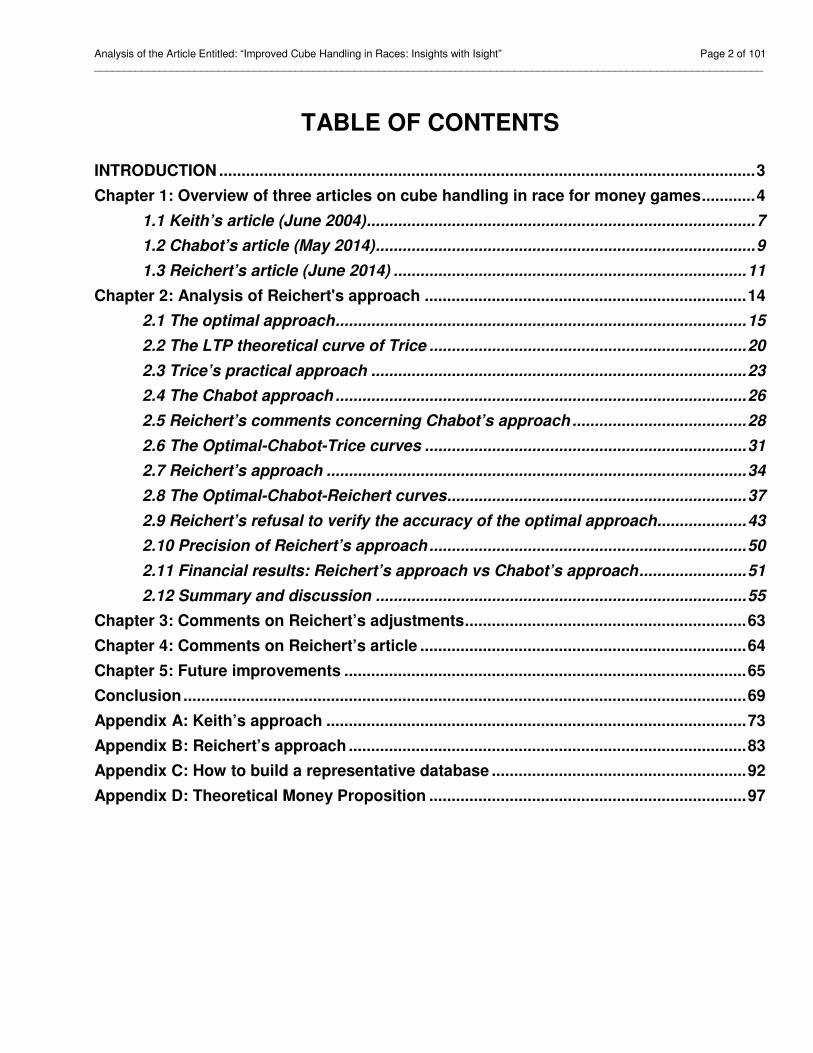
TABLE OF CONTENTS
INTRODUCTION ........................................................................................................................ 3
Chapter 1: Overview of three articles on cube handling in race for money games ............ 4
1.1 Keith’s article (June 2004) ....................................................................................... 7
1.2 Chabot’s article (May 2014) ..................................................................................... 9
1.3 Reichert’s article (June 2014) ............................................................................... 11
Chapter 2: Analysis of Reichert's approach ........................................................................ 14
2.1 The optimal approach ............................................................................................ 15
2.2 The LTP theoretical curve of Trice ....................................................................... 20
2.3 Trice’s practical approach .................................................................................... 23
2.4 The Chabot approach ............................................................................................ 26
2.5 Reichert’s comments concerning Chabot’s approach ....................................... 28
2.6 The Optimal-Chabot-Trice curves ........................................................................ 31
2.7 Reichert’s approach .............................................................................................. 34
2.8 The Optimal-Chabot-Reichert curves ................................................................... 37
2.9 Reichert’s refusal to verify the accuracy of the optimal approach .................... 43
2.10 Precision of Reichert’s approach ....................................................................... 50
2.11 Financial results: Reichert’s approach vs Chabot’s approach ........................ 51
2.12 Summary and discussion ................................................................................... 55
Chapter 3: Comments on Reichert’s adjustments ............................................................... 63
Chapter 4: Comments on Reichert’s article ......................................................................... 64
Chapter 5: Future improvements .......................................................................................... 65
Conclusion .............................................................................................................................. 69
Appendix A: Keith’s approach .............................................................................................. 73
Appendix B: Reichert’s approach ......................................................................................... 83
Appendix C: How to build a representative database ......................................................... 92
Appendix D: Theoretical Money Proposition ....................................................................... 97

Analysis of the Article Entitled: “Improved Cube Handling in Races: Insights with Isight” Page 3 of 101 _________________________________________________________________________________________________________________
INTRODUCTION In May 2014, I published an article entitled: “Money Cube Action in Low-wastage Positions.” That article presented a theoretical approach called the optimal approach and a practical approach called Chabot's approach. In June 2014, Axel Reichert published his article entitled: “Improved Cube Handling in Races: Insights with Isight”. Here is his summary of his own article:
After looking into how adjusted pip counts and decision criteria work in general, we present a more formal framework that allows us to parameterize and optimize adjusted pip counts and the corresponding decision criteria. The outcome is a new method resulting in both less effort and fewer errors for your cube handling in races compared to existing methods.
Reichert has incorrectly concluded that the new proposed decision criteria are the best ones proposed so far. In fact, the technique used by Reichert to develop new decision criteria contains three major flaws. Consequently, his decision criteria are rather the worst ones proposed so far. Chapter 1 is entitled: “Overview of three articles on cube handling in race for money games”. This chapter presents three (3) articles, namely: an article published by Tom Keith (in June 2004), an article published by Michelin Chabot (in May 2014), and an article published by Axel Reichert (in June 2014). Chapter 2, entitled “Analysis of Reichert's approach”, explains what are the three flaws committed by Reichert while developing his decision criteria. It then explains why Reichert’s decision criteria are the worst decision criteria presented so far. Chapter 3, entitled “Comments on Reichert's adjustments”, comments about Reichert’s adjustments. Chapter 4, entitled “Comments on Reichert's article”, comments about all others topics developed in Reichert’s article, excluding Reichert's approach and Reichert's adjustment. Chapter 5, entitled “Future improvements”, gives suggestions to improve the existing theory of cube handling in race for money games. The main goal of this article is to clearly explain:
• what are the three flaws that Reichert committed to develop his decision criteria; and,
• why Reichert’s decision criteria are the worst decision criteria proposed so far.
The secondary goal of this article is to give some suggestions on how to further improve the existing theory on cube handling in race for money games.
+ + + + +

Analysis of the Article Entitled: “Improved Cube Handling in Races: Insights with Isight” Page 4 of 101 _________________________________________________________________________________________________________________
Chapter 1: Overview of three articles on cube handling in race for money games The purpose of this chapter is to present three articles on cube handling in race for money games, namely:
• Keith’s article (June 2004) • Chabot’s article (May 2014
• Reichert’s article (June 2014) The first article presented, which was published in June 2004, is that of Tom Keith. His article is entitled: “Cube Handling in Noncontact Positions”. Hereinafter, Tom Keith will be called Keith. The article published by Keith will be called Keith's article. As proposed by Keith, the adjustments to do in order to obtain an adjusted pipcount will be called Keith's adjustments. The decision criteria proposed by Keith will be called Keith’s approach.
The second article presented, which was published in May 2014, is my own article. That article is entitled: “Money Cube Action in Low-Wastage Position”. In November 2014, that article has been slightly modified but the content remains essentially unchanged. Hereinafter, Michelin Chabot will be called Chabot. That article will be called Chabot’s article. There are no Chabot adjustments because none are proposed in that article. The decision criteria proposed will be called Chabot's approach.
The third article presented, which was published in June 2014, is that of Axel Reichert. His article is entitled: “Improved Cube Handling in Races: Insights with Isight”. Hereinafter, Axel Reichert will be called Reichert. The article published by Reichert will be called Reichert’s article. As proposed by Reichert, the adjustments to do in order to obtain an adjusted pip count will be called Reichert’s adjustments. The decision criteria proposed by Reichert will be called Reichert’s approach. The combination of Reichert’s adjustments and approach will be called Reichert’s method. In his article, Reichert named his method the “Isight method”. However, in this article, Reichert's method will be called as is.
Chabot's article elaborates exclusively on cube handling in race for money games. Even if Keith's article and Reichert's article develop topics other than cube handling in race for money games; the only subject developed in this present article relates to cube handling in race for money games.
Analysis of the Article Entitled: “Improved Cube Handling in Races: Insights with Isight” Page 5 of 101 _________________________________________________________________________________________________________________
The three previously mentioned articles will be presented using exactly the same presentation. The presentation includes the eight (8) following steps:
1) The first step is to give an internet link to allow you to view the article in question.
2) The second step is to locate in which section of their respective article the approach was analyzed. It should be noted that the three approaches were analyzed using exactly the same technique that is presented in Section 2.1 of Chabot's article (pages 49 and 50 of Chabot's article).
3) The third step is to present the summary of the article. This presentation is made using the relevant excerpt which is usually located at the beginning of each article.
4) The fourth step is to comment the quality of the databases used in order to obtain the proposed adjustments and the proposed approach. Appendix C, entitled: “How to build a representative database”, explains the difference between an unrepresentative database, a representative database and a very representative database.
5) The fifth step is to present the proposed adjustments in order to get the adjusted pipcount. The adjusted pipcount is obtained by first calculating the “straight” pipcount and adding the adjustments. To use an approach, it is necessary to have the adjusted pipcount of both players.
6) The sixth step is to present the approach, that is to say, to present the proposed decision criteria to follow in order to determine if a player should double or not, redouble or not, take or pass. The approach is presented using exactly the same terms as those used by the authors. For Chabot's approach, there is no sixth step because Chabot's approach is only presented by using mathematical formulas.
7) The seventh step is to present the approach by using mathematical formulas. An approach is to use three (3) mathematical formulas, namely:
• one (1) formula for the DP (Doubling Point);
• one (1) formula for the RP (Redoubling Point); and, • one (1) formula for the LTP (Last Take Point).
With regard to Keith’s approach, to obtain the mathematical formulas, it has been necessary to transform the presented text into mathematical formulas.
With regard to Chabot's approach, the mathematical formulas to be used had already been presented in Chabot's article.
Analysis of the Article Entitled: “Improved Cube Handling in Races: Insights with Isight” Page 6 of 101 _________________________________________________________________________________________________________________
With regard to Reichert’s approach, the situation is a little more difficult to explain because Reichert has proposed two different techniques to obtain Reichert's approach. Both techniques presented give exactly the same results. The first technique is called “the general technique” and the second technique is called “the specific technique”. The general technique can be used for match games and money games, while the specific technique can only be used for money games. For the general technique, Reichert already presented mathematical formulas, but for the specific technique, Reichert has not presented mathematical formulas. So, to obtain the mathematical formulas for the specific technique, it has been necessary to transform the presented text into mathematical formulas.
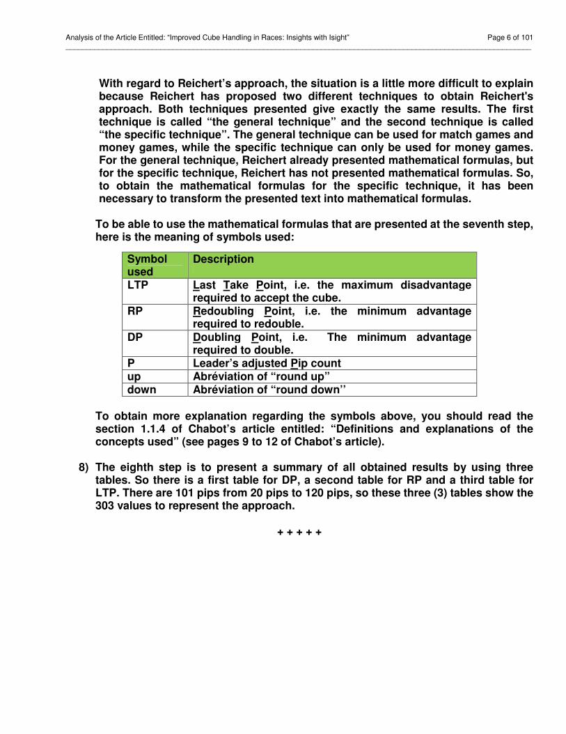
To be able to use the mathematical formulas that are presented at the seventh step, here is the meaning of symbols used: To obtain more explanation regarding the symbols above, you should read the section 1.1.4 of Chabot’s article entitled: “Definitions and explanations of the concepts used” (see pages 9 to 12 of Chabot’s article).
8) The eighth step is to present a summary of all obtained results by using three tables. So there is a first table for DP, a second table for RP and a third table for LTP. There are 101 pips from 20 pips to 120 pips, so these three (3) tables show the 303 values to represent the approach.
+ + + + +
Symbol used
Description
LTP Last Take Point, i.e. the maximum disadvantage required to accept the cube.
RP Redoubling Point, i.e. the minimum advantage required to redouble.
DP Doubling Point, i.e. The minimum advantage required to double.
P Leader’s adjusted Pip count up Abréviation of “round up” down Abréviation of “round down’’

Analysis of the Article Entitled: “Improved Cube Handling in Races: Insights with Isight” Page 7 of 101 _________________________________________________________________________________________________________________
1.1 Keith’s article (June 2004)
Keith's article is presented on the website Backgammon Galore! at the following link: http://www.bkgm.com/articles/CubeHandlingInRaces/.
The analysis of Keith's approach is presented in Appendix A of that article.
The summary of Keith's article is presented at the beginning of his article. Here is the relevant excerpt:
“In this article I describe and evaluate several popular methods of making cube decisions in noncontact positions. To compare the methods, I use real positions from real games. In this way, the types of positions which occur often in actual play are weighed more heavily than positions that happen only rarely. All positions were rolled out by computer to obtain accurate cubeless and cubeful equities.
Five different pip-adjusting formulas are evaluated; the Thorp count, the Keeler/Gillogly count, the Ward count, the Lamford/Gasquoine count, and my own "Keith" count. The formulas are judged on their ability to account for wastage and on their ability to make accurate cube decisions.
Finally, I give some information on converting between cubeless and cubeful equity.”
To obtain Keith’s adjustments and Keith’s approach; the used database is an unrepresentative database. Indeed, it is clearly mentioned in the above extract.
Here are Keith’s adjustments:
• add 2 pips for each checker more than 1 on the one point; • add 1 pip for each checker more than 1 on the two point;
• add 1 pip for each checker more than 3 on the three point; • add 1 pip for each empty space on points four, five, and six.
Here is Keith’s approach:
• Increase the count of the player on roll by one-seventh (rounding down).
• A player should double if his count exceeds the opponent's count by no more than 4.
• A player should redouble if his count exceeds the opponent's count by no more than 3.
• The opponent should take if the doubler's count exceeds the opponent's count by at least 2.
Analysis of the Article Entitled: “Improved Cube Handling in Races: Insights with Isight” Page 8 of 101 _________________________________________________________________________________________________________________
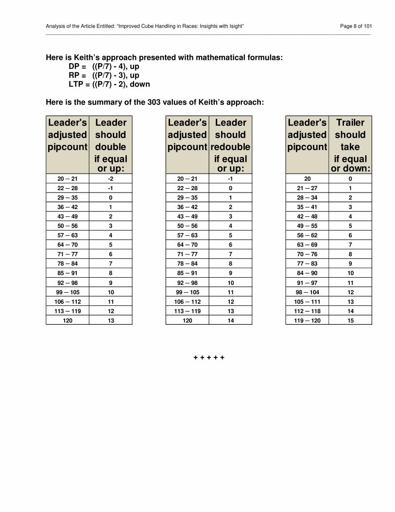
Here is Keith’s approach presented with mathematical formulas: DP = ((P/7) - 4), up RP = ((P/7) - 3), up LTP = ((P/7) - 2), down
Here is the summary of the 303 values of Keith’s approach:
+ + + + +
Leader's Leader Leader's Leader Leader's Trailer
adjusted should adjusted should adjusted should
pipcount double pipcount redouble pipcount take
if equal if equal if equalor up: or up: or down:
20 ─ 21 -2 20 ─ 21 -1 20 0
22 ─ 28 -1 22 ─ 28 0 21 ─ 27 1
29 ─ 35 0 29 ─ 35 1 28 ─ 34 2
36 ─ 42 1 36 ─ 42 2 35 ─ 41 3
43 ─ 49 2 43 ─ 49 3 42 ─ 48 4
50 ─ 56 3 50 ─ 56 4 49 ─ 55 5
57 ─ 63 4 57 ─ 63 5 56 ─ 62 6
64 ─ 70 5 64 ─ 70 6 63 ─ 69 7
71 ─ 77 6 71 ─ 77 7 70 ─ 76 8
78 ─ 84 7 78 ─ 84 8 77 ─ 83 9
85 ─ 91 8 85 ─ 91 9 84 ─ 90 10
92 ─ 98 9 92 ─ 98 10 91 ─ 97 11
99 ─ 105 10 99 ─ 105 11 98 ─ 104 12
106 ─ 112 11 106 ─ 112 12 105 ─ 111 13
113 ─ 119 12 113 ─ 119 13 112 ─ 118 14
120 13 120 14 119 ─ 120 15
Analysis of the Article Entitled: “Improved Cube Handling in Races: Insights with Isight” Page 9 of 101 _________________________________________________________________________________________________________________
1.2 Chabot’s article (May 2014)
Chabot's article is presented on the website Backgammon Galore! at the following link: http://www.bkgm.com/articles/Chabot/MoneyCubeAction.pdf.
The analysis of Chabot's approach is presented at the section 2.6 of Chabot's article (pages 77 to 83 of Chabot's article).
The summary of Chabot's article is presented in the introduction. Here is the relevant excerpt:
“The general purpose of this article is to elaborate the doubling cube theory in money games, for running positions, in which there is little or no wastage.
The specific purposes of this article are:
• To present the optimal approach. • To analyze three known approaches proposed so far.
• To propose a new approach.
This article includes 3 parts:
• Part 1 entitled: “The optimal approach”, begins by giving the definitions and explanations of all the concepts that will be used in this article. This first part also presents in great detail, the technique used to develop the optimal approach. This part was written to allow a sceptical reader to be able to verify this technique, and to be able to confirm that the obtained approach is really the optimal one.
• Part 2 entitled: “Analysis of some approaches”, analyzes three known approaches proposed so far, namely: the 8%. 9%, 12% approach, Thorp’s approach and Trice’s approach. This part also proposes a new approach, namely: the Chabot one.
• Part 3 entitled: "From theory to practice", mainly explains, with the help of a few practical examples, how to use the recommendable approaches.”
In Chabot’s article, it is clearly mentioned that Chabot’s approach is based on the optimal approach. To obtain the optimal approach, the database used contains 51 positions, namely: 20 pips, 22 pips, 24 pips, … , 116 pips, 118 pips and 120 pips. All analyzed positions were “low-wastage position” that meet some specific criteria which were enumerated in section 1.1.3 of Chabot’s article. So, to develop the optimal approach, the database used was a very representative database, and consequently, Chabot’s approach was also obtained based on the same very representative database.
Chabot’s article does not propose any adjustment to obtain an adjusted pip count.
Analysis of the Article Entitled: “Improved Cube Handling in Races: Insights with Isight” Page 10 of 101 _________________________________________________________________________________________________________________
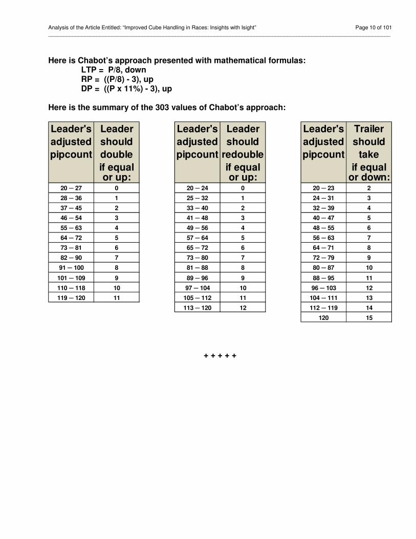
Here is Chabot’s approach presented with mathematical formulas: LTP = P/8, down RP = ((P/8) - 3), up DP = ((P x 11%) - 3), up
Here is the summary of the 303 values of Chabot’s approach:
+ + + + +
Leader's Leader Leader's Leader Leader's Trailer
adjusted should adjusted should adjusted should
pipcount double pipcount redouble pipcount take
if equal if equal if equalor up: or up: or down:
20 ─ 27 0 20 ─ 24 0 20 ─ 23 2
28 ─ 36 1 25 ─ 32 1 24 ─ 31 3
37 ─ 45 2 33 ─ 40 2 32 ─ 39 4
46 ─ 54 3 41 ─ 48 3 40 ─ 47 5
55 ─ 63 4 49 ─ 56 4 48 ─ 55 6
64 ─ 72 5 57 ─ 64 5 56 ─ 63 7
73 ─ 81 6 65 ─ 72 6 64 ─ 71 8
82 ─ 90 7 73 ─ 80 7 72 ─ 79 9
91 ─ 100 8 81 ─ 88 8 80 ─ 87 10
101 ─ 109 9 89 ─ 96 9 88 ─ 95 11
110 ─ 118 10 97 ─ 104 10 96 ─ 103 12
119 ─ 120 11 105 ─ 112 11 104 ─ 111 13
113 ─ 120 12 112 ─ 119 14
120 15
Analysis of the Article Entitled: “Improved Cube Handling in Races: Insights with Isight” Page 11 of 101 _________________________________________________________________________________________________________________
1.3 Reichert’s article (June 2014) Reichert's article is presented on the website Backgammon Galore! at the following link: http://www.bkgm.com/articles/Reichert/insights-with-isight.pdf.
The analysis of Reichert's approach is presented in Appendix B of this article.
The summary of Reichert's article is presented in his introduction. Here is the relevant extract:
“After having a look into how adjusted pip counts and approach work in general, we will then proceed to a more formal framework that will allow us to parameterize and optimize adjusted pip counts and the corresponding approach. The outcome will be a new method (or, more precisely, several new methods) resulting in both less effort and fewer errors for your cube handling in races compared to existing methods (Thorp, Keeler, Ward, Keith, Matussek, Kleinman, Trice, Ballard etc.). Such a claim demands verification, hence we will look at results obtained with the new method and compare them to the existing ones for cube handling in races. Furthermore we will look at approximations of the effective pip count (EPC) or the cubeless probability of winning (CPW), which is a prerequisite of methods for match play. A summary concludes this article and recapitulates my findings for the impatient backgammon player who is always on the run, since the next race is in line online. Finally, the appendices contain several examples detailing the application of the new method and, for the readers not yet convinced of its merits, some rather technical remarks and further comparisons.”
To obtain Reichert’s adjustments and Reichert’s approach; the used database is an unrepresentative database. Indeed, it is clearly mentioned on page 39 of the Reichert’s article. See also the appendix C entitled: “How to build a representative database”.
Here are Reichert’s adjustments: • Add 1 pip for each additional checker on the board compared to the
opponent.
• Add 2 pips for each checker more than 2 on point 1. • Add 1 pip for each checker more than 2 on point 2.
• Add 1 pip for each checker more than 3 on point 3. • Add 1 pip for each empty space on points 4, 5, or 6 (only if the other
player has a checker on his corresponding point).
• Add 1 pip for each additional crossover compared to the opponent.
Analysis of the Article Entitled: “Improved Cube Handling in Races: Insights with Isight” Page 12 of 101 _________________________________________________________________________________________________________________
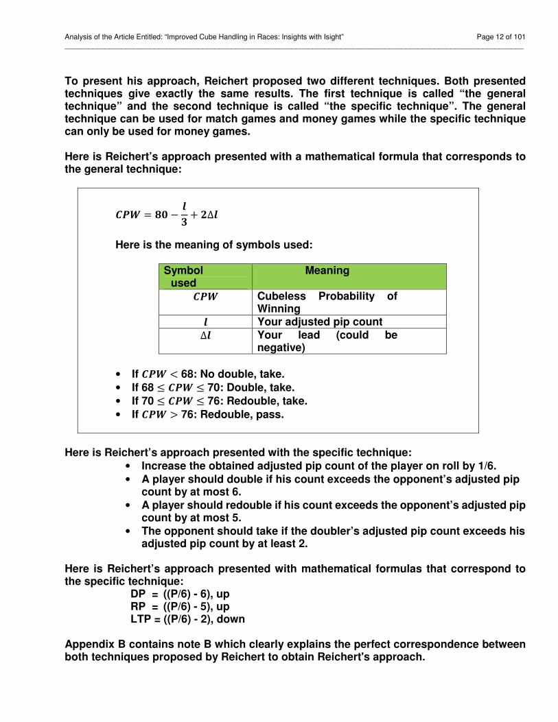
To present his approach, Reichert proposed two different techniques. Both presented techniques give exactly the same results. The first technique is called “the general technique” and the second technique is called “the specific technique”. The general technique can be used for match games and money games while the specific technique can only be used for money games. Here is Reichert’s approach presented with a mathematical formula that corresponds to the general technique:
��� = �� −�
+ �∆�
Here is the meaning of symbols used:
Symbol
used Meaning
��� Cubeless Probability of Winning
� Your adjusted pip count
∆� Your lead (could be negative)
• If ��� < 68: No double, take.
• If 68 ≤ ��� ≤ 70: Double, take.
• If 70 ≤ ��� ≤ 76: Redouble, take.
• If ��� > 76: Redouble, pass.
Here is Reichert’s approach presented with the specific technique:
• Increase the obtained adjusted pip count of the player on roll by 1/6.
• A player should double if his count exceeds the opponent’s adjusted pip count by at most 6.
• A player should redouble if his count exceeds the opponent’s adjusted pip count by at most 5.
• The opponent should take if the doubler’s adjusted pip count exceeds his adjusted pip count by at least 2.
Here is Reichert’s approach presented with mathematical formulas that correspond to the specific technique:
DP = ((P/6) - 6), up RP = ((P/6) - 5), up LTP = ((P/6) - 2), down
Appendix B contains note B which clearly explains the perfect correspondence between both techniques proposed by Reichert to obtain Reichert's approach.

Analysis of the Article Entitled: “Improved Cube Handling in Races: Insights with Isight” Page 13 of 101 _________________________________________________________________________________________________________________
Here is the summary of all 303 values of Reichert’s approach:
+ + + + +
Leader's Leader Leader's Leader Leader's Trailer
adjusted should adjusted should adjusted should
pipcount double pipcount redouble pipcount take
if equal if equal if equalor up: or up: or down:
20 ─ 24 -2 20 ─ 24 -1 20 ─ 23 1
25 ─ 30 -1 25 ─ 30 0 24 ─ 29 2
31 ─ 36 0 31 ─ 36 1 30 ─ 35 3
37 ─ 42 1 37 ─ 42 2 36 ─ 41 4
43 ─ 48 2 43 ─ 48 3 42 ─ 47 5
49 ─ 54 3 49 ─ 54 4 48 ─ 53 6
55 ─ 60 4 55 ─ 60 5 54 ─ 59 7
61 ─ 66 5 61 ─ 66 6 60 ─ 65 8
67 ─ 72 6 67 ─ 72 7 66 ─ 71 9
73 ─ 78 7 73 ─ 78 8 72 ─ 77 10
79 ─ 84 8 79 ─ 84 9 78 ─ 83 11
85 ─ 90 9 85 ─ 90 10 84 ─ 89 12
91 ─ 96 10 91 ─ 96 11 90 ─ 95 13
97 ─ 102 11 97 ─ 102 12 96 ─ 101 14
103 ─ 108 12 103 ─ 108 13 102 ─ 107 15
109 ─ 114 13 109 ─ 114 14 108 ─ 113 16
115 ─ 120 14 115 ─ 120 15 114 ─ 119 17
120 18
Analysis of the Article Entitled: “Improved Cube Handling in Races: Insights with Isight” Page 14 of 101 _________________________________________________________________________________________________________________
Chapter 2: Analysis of Reichert's approach In June 2014, Axel Reichert published an article entitled “Improved Handling Cube in Race: Insight with Isight”. Here is his summary of his own article:
After looking into how adjusted pip counts and decision criteria work in general, we present a more formal framework that allows us to parameterize and optimize adjusted pip counts and the corresponding decision criteria. The outcome is a new method resulting in both less effort and fewer errors for your cube handling in races compared to existing methods.
Reichert has incorrectly concluded that the new proposed decision criteria are the best ones proposed so far. In fact, the technique used by Reichert to develop new decision criteria contains three major flaws. Consequently, his decision criteria are rather the worst ones proposed so far. As already mentioned, hereafter, Reichert’s decision criteria will be called Reichert’s approach. The main goal of this chapter is to clearly explain what are the three flaws committed by Reichert while developing his decision criteria and why Reichert’s approach is the worst approach presented so far. This chapter includes the following sections:
2.1 The optimal approach 2.2 The LTP theoretical curve of Trice 2.3 Trice’s practical approach 2.4 Chabot’s approach 2.5 Reichert’s comments concerning Chabot’s approach 2.6 The Optimal-Chabot-Trice curves 2.7 Reichert’s approach 2.8 The Optimal-Chabot-Reichert curves 2.9 Reichert’s refusal to verify the accuracy of the optimal approach 2.10 Precision of the Reichert’s approach 2.11 Financial results: Reichert’s approach vs Chabot’s approach 2.12 Summary and discussion
+ + + + +

Analysis of the Article Entitled: “Improved Cube Handling in Races: Insights with Isight” Page 15 of 101 _________________________________________________________________________________________________________________
2.1 The optimal approach The optimal approach is elaborated in part 1 of Chabot’s article (see pages 5 to 48 of Chabot’s article). Chabot’s article explains in a very detailed way the technique used to develop the optimal approach. Indeed, the technique is presented in a very detailed way to allow any skeptical reader to verify this technique and to be able to confirm that the obtained approach is really the optimal one. Here is a summary of the technique used to develop the optimal approach:
• To obtain the optimal approach, the database used contains 51 positions, namely: 20 pips, 22 pips, 24 pips, … , 116 pips, 118 pips and 120 pips. All analyzed position were “low-wastage position” that meet some specifics criteria which were enumerated in section 1.1.3 of Chabot’s article.
• For each position, there are 3 results (i.e. LTP, RP and DP), so this represents 153 results (i.e. 51 positions x 3 results/position).
• To obtain each result, it was necessary to obtain 4 values. Indeed, to obtain each result, it was necessary to find the intersection between two (2) straight lines. To define each straight line, it was necessary to have two (2) values. So this represents 712 values (i.e. 153 results x 4 values/result).
• Each value has been evaluated with great precision. The type of evaluation used is: “Full Cubefull Rollout, 3-Ply Play, 3-Ply Cube” in order to obtain a precision (or a “95% confidence interval”) better than 0.040 “Normalized point per games”. Such precision correspond to an equivalent of a minimun of 25,000 games.
• For example, when the Leader’s pip count is 100 pips; the obtained theoretical value for the LTP point is 12.10 pips. This value is presented in Table 3 (See page 28 of Chabot’s article). This value is the intersection of the “Double, Take” curve, with the “Double, Pass” curve (See page 33 of the Chabot’s article). To find the value of this intersection, it was necessary to use the mathematical technique explained in the Appendix 3 of the Chabot’s article (See page 46 of the Chabot’s article). So, if the obtained value is 12.10 pips, it was because 12 pips is a take; and 13 pips is a pass.
The optimal approach was obtained using 712 very representative values. Therefore, the database used was a very representative database. Consequently, the optimal approach is a very reliable approach.

Analysis of the Article Entitled: “Improved Cube Handling in Races: Insights with Isight” Page 16 of 101 _________________________________________________________________________________________________________________
The optimal approach is presented in section 2.2 entitled: “Optimal approach” (see pages 51 to page 55 of Chabot’s article). This approach is summarized in table 2.2 (see page 53 of Chabot’s article). Table 2.2 is reproduced hereunder:
Table 2.2: Summary of the obtained values for the optimal approach
Leader's Leader Leader's Leader Leader's Trailer
adjusted should adjusted should adjusted should
pipcount double pipcount redouble pipcount take
if equal if equal if equal
or up: or up: or down:20 ─ 23 -1 20 -1 20 ─ 24 2
24 ─ 30 0 21 ─ 26 0 25 ─ 30 3
31 ─ 37 1 27 ─ 32 1 31 ─ 37 4
38 ─ 45 2 33 ─ 38 2 38 ─ 45 5
46 ─ 54 3 39 ─ 45 3 46 ─ 52 6
55 ─ 64 4 46 ─ 52 4 53 ─ 60 7
65 ─ 74 5 53 ─ 60 5 61 ─ 68 8
75 ─ 85 6 61 ─ 68 6 69 ─ 77 9
86 ─ 95 7 69 ─ 76 7 78 ─ 86 10
96 ─ 106 8 77 ─ 85 8 87 ─ 95 11
107 ─ 115 9 86 ─ 96 9 96 ─ 105 12
116 ─ 120 10 97 ─ 108 10 106 ─ 116 13
109 ─ 120 11 117 ─ 120 14
Analysis of the Article Entitled: “Improved Cube Handling in Races: Insights with Isight” Page 17 of 101 _________________________________________________________________________________________________________________
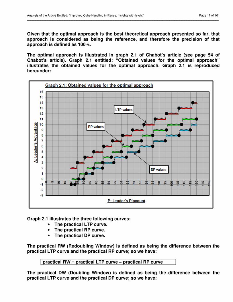
Given that the optimal approach is the best theoretical approach presented so far, that approach is considered as being the reference, and therefore the precision of that approach is defined as 100%. The optimal approach is illustrated in graph 2.1 of Chabot’s article (see page 54 of Chabot’s article). Graph 2.1 entitled: “Obtained values for the optimal approach” illustrates the obtained values for the optimal approach. Graph 2.1 is reproduced hereunder:
Graph 2.1 illustrates the three following curves:
• The practical LTP curve. • The practical RP curve.
• The practical DP curve. The practical RW (Redoubling Window) is defined as being the difference between the practical LTP curve and the practical RP curve; so we have:
practical RW = practical LTP curve – practical RP curve
The practical DW (Doubling Window) is defined as being the difference between the practical LTP curve and the practical DP curve; so we have:
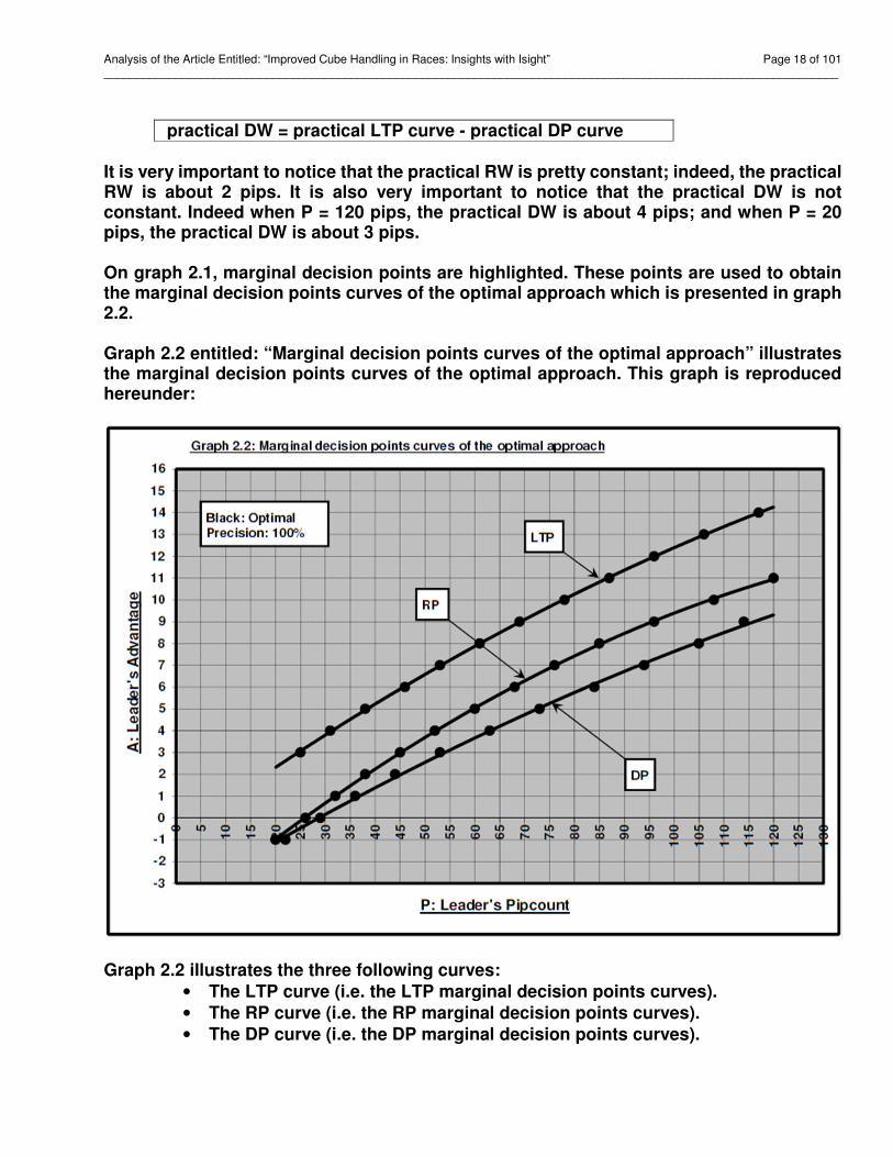
Analysis of the Article Entitled: “Improved Cube Handling in Races: Insights with Isight” Page 18 of 101 _________________________________________________________________________________________________________________
practical DW = practical LTP curve - practical DP curve It is very important to notice that the practical RW is pretty constant; indeed, the practical RW is about 2 pips. It is also very important to notice that the practical DW is not constant. Indeed when P = 120 pips, the practical DW is about 4 pips; and when P = 20 pips, the practical DW is about 3 pips. On graph 2.1, marginal decision points are highlighted. These points are used to obtain the marginal decision points curves of the optimal approach which is presented in graph 2.2. Graph 2.2 entitled: “Marginal decision points curves of the optimal approach” illustrates the marginal decision points curves of the optimal approach. This graph is reproduced hereunder:
Graph 2.2 illustrates the three following curves:
• The LTP curve (i.e. the LTP marginal decision points curves).
• The RP curve (i.e. the RP marginal decision points curves). • The DP curve (i.e. the DP marginal decision points curves).
Analysis of the Article Entitled: “Improved Cube Handling in Races: Insights with Isight” Page 19 of 101 _________________________________________________________________________________________________________________
The RW (Redoubling Window) is defined as being the difference between the LTP curve and the RP curve; so we have:
RW = LTP curve - RP curve The DW (Doubling Window) is defined as being the difference between the LTP curve and the DP curve; so we have:
DW = LTP curve - DP curve It is very important to notice that the RW is pretty constant; indeed, the RW is about 3 pips. It is also very important to notice that the DW is not constant. Indeed when P = 120 pips, the DW is about 5 pips; and when P = 20 pips, the DW is about 3 pips.
+ + + + +
Analysis of the Article Entitled: “Improved Cube Handling in Races: Insights with Isight” Page 20 of 101 _________________________________________________________________________________________________________________
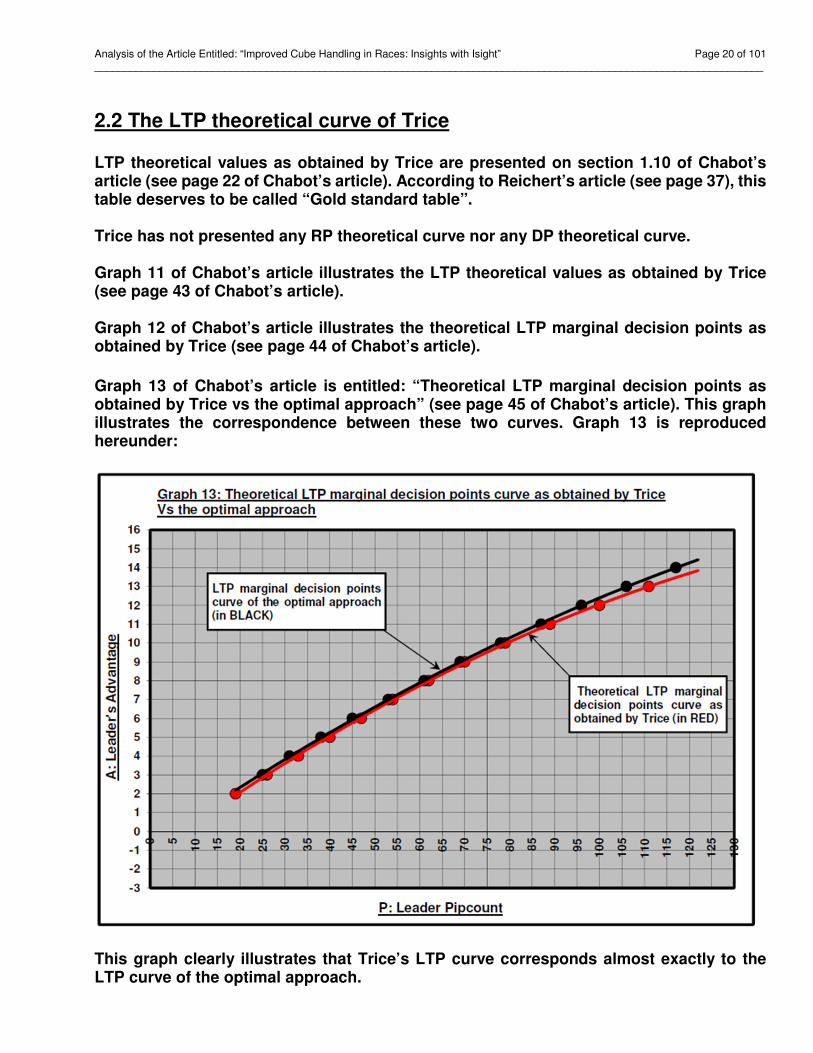
2.2 The LTP theoretical curve of Trice LTP theoretical values as obtained by Trice are presented on section 1.10 of Chabot’s article (see page 22 of Chabot’s article). According to Reichert’s article (see page 37), this table deserves to be called “Gold standard table”. Trice has not presented any RP theoretical curve nor any DP theoretical curve. Graph 11 of Chabot’s article illustrates the LTP theoretical values as obtained by Trice (see page 43 of Chabot’s article). Graph 12 of Chabot’s article illustrates the theoretical LTP marginal decision points as obtained by Trice (see page 44 of Chabot’s article).
Graph 13 of Chabot’s article is entitled: “Theoretical LTP marginal decision points as obtained by Trice vs the optimal approach” (see page 45 of Chabot’s article). This graph illustrates the correspondence between these two curves. Graph 13 is reproduced hereunder:
This graph clearly illustrates that Trice’s LTP curve corresponds almost exactly to the LTP curve of the optimal approach.
Analysis of the Article Entitled: “Improved Cube Handling in Races: Insights with Isight” Page 21 of 101 _________________________________________________________________________________________________________________
The fact that the theoretical LTP marginal decision points curve as obtained by Trice corresponds almost exactly to the theoretical LTP marginal decision points curve of the optimal approach is probably not a coincidence. This confirms that Walter Trice had probably obtained his theoretical approach using certain computational technique pretty similar to the technique that is explained in a very exhaustive way in Chabot’s article. However, it is possible that Walter Trice made certain visual evaluations, whereas the optimal approach has been obtained without any visual evaluations.
+ + + + +

Analysis of the Article Entitled: “Improved Cube Handling in Races: Insights with Isight” Page 22 of 101 _________________________________________________________________________________________________________________
The precision of Trice’s LTP theoretical curve is 75%. Here is the calculation of the precision of Trice’s LTP theoretical curve:
+ + + + +
P LTP opt LTP Trice Gap P LTP opt LTP Trice Gap
20 2 2 0 71 9 9 0
21 2 2 0 72 9 9 0
22 2 2 0 73 9 9 0
23 2 2 0 74 9 9 0
24 2 2 0 75 9 9 0
25 3 2 1 76 9 9 0
26 3 3 0 77 9 9 0
27 3 3 0 78 10 9 1
28 3 3 0 79 10 10 0
29 3 3 0 80 10 10 0
30 3 3 0 81 10 10 0
31 4 3 1 82 10 10 0
32 4 3 1 83 10 10 0
33 4 4 0 84 10 10 0
34 4 4 0 85 10 10 0
35 4 4 0 86 10 10 0
36 4 4 0 87 11 10 1
37 4 4 0 88 11 10 1
38 5 4 1 89 11 11 0
39 5 4 1 90 11 11 0
40 5 5 0 91 11 11 0
41 5 5 0 92 11 11 0
42 5 5 0 93 11 11 0
43 5 5 0 94 11 11 0
44 5 5 0 95 11 11 0
45 5 5 0 96 12 11 1
46 6 5 1 97 12 11 1
47 6 6 0 98 12 11 1
48 6 6 0 99 12 11 1
49 6 6 0 100 12 12 0
50 6 6 0 101 12 12 0
51 6 6 0 102 12 12 0
52 6 6 0 103 12 12 0
53 7 6 1 104 12 12 0
54 7 7 0 105 12 12 0
55 7 7 0 106 13 12 1
56 7 7 0 107 13 12 1
57 7 7 0 108 13 12 1
58 7 7 0 109 13 12 1
59 7 7 0 110 13 12 1
60 7 7 0 111 13 13 0
61 8 7 1 112 13 13 0
62 8 8 0 113 13 13 0
63 8 8 0 114 13 13 0
64 8 8 0 115 13 13 0
65 8 8 0 116 13 13 0
66 8 8 0 117 14 13 1
67 8 8 0 118 14 13 1
68 8 8 0 119 14 13 1
69 9 8 1 120 14 13 1
70 9 9 0
Good results 76 on 101 = 75.2% Results with a 1-pip difference 25 on 101 = 24.8%
Analysis of the Article Entitled: “Improved Cube Handling in Races: Insights with Isight” Page 23 of 101 _________________________________________________________________________________________________________________
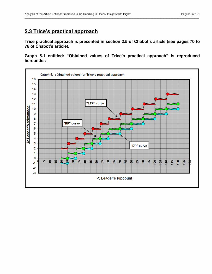
2.3 Trice’s practical approach Trice practical approach is presented in section 2.5 of Chabot’s article (see pages 70 to 76 of Chabot’s article). Graph 5.1 entitled: “Obtained values of Trice’s practical approach” is reproduced hereunder:
Analysis of the Article Entitled: “Improved Cube Handling in Races: Insights with Isight” Page 24 of 101 _________________________________________________________________________________________________________________
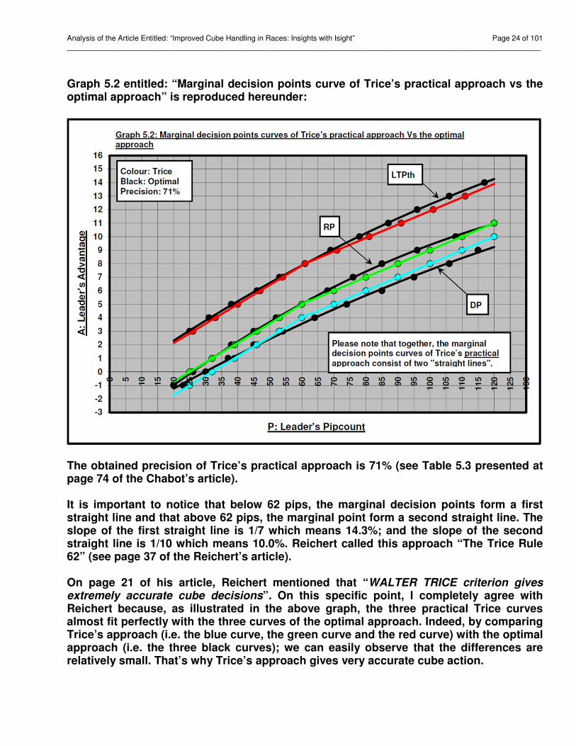
Graph 5.2 entitled: “Marginal decision points curve of Trice’s practical approach vs the optimal approach” is reproduced hereunder:
The obtained precision of Trice’s practical approach is 71% (see Table 5.3 presented at page 74 of the Chabot’s article). It is important to notice that below 62 pips, the marginal decision points form a first straight line and that above 62 pips, the marginal point form a second straight line. The slope of the first straight line is 1/7 which means 14.3%; and the slope of the second straight line is 1/10 which means 10.0%. Reichert called this approach “The Trice Rule 62” (see page 37 of the Reichert’s article). On page 21 of his article, Reichert mentioned that “WALTER TRICE criterion gives extremely accurate cube decisions”. On this specific point, I completely agree with Reichert because, as illustrated in the above graph, the three practical Trice curves almost fit perfectly with the three curves of the optimal approach. Indeed, by comparing Trice’s approach (i.e. the blue curve, the green curve and the red curve) with the optimal approach (i.e. the three black curves); we can easily observe that the differences are relatively small. That’s why Trice’s approach gives very accurate cube action.

Analysis of the Article Entitled: “Improved Cube Handling in Races: Insights with Isight” Page 25 of 101 _________________________________________________________________________________________________________________
In Chabot’s article, I had to conclude that Trice’s approach could not be recommended because this approach is too difficult to remember and too difficult to use (see page 96 of Chabot’s article). In his article, Reichert also mentioned that Trice’s approach with a “distinction between long and short race” requires too much effort to be used (see page 39 and 40 of Reichert’s article). On this specific subject, I also fully agree with Reichert.
+ + + + +
Analysis of the Article Entitled: “Improved Cube Handling in Races: Insights with Isight” Page 26 of 101 _________________________________________________________________________________________________________________
2.4 The Chabot approach
To develop Chabot’s approach, the goal was to obtain an approach giving the best practical approach which meets the three (3) following requirements:
• This approach must give the best possible precision using the optimal approach as reference.
• The obtained precision must be higher than the precision obtained by Thorp’s approach (which is 53%).
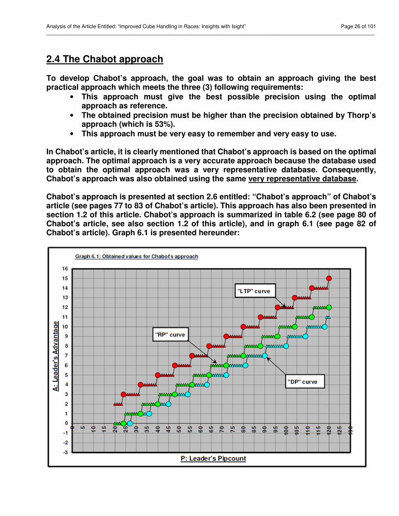
• This approach must be very easy to remember and very easy to use. In Chabot’s article, it is clearly mentioned that Chabot’s approach is based on the optimal approach. The optimal approach is a very accurate approach because the database used to obtain the optimal approach was a very representative database. Consequently, Chabot’s approach was also obtained using the same very representative database. Chabot’s approach is presented at section 2.6 entitled: “Chabot’s approach” of Chabot’s article (see pages 77 to 83 of Chabot’s article). This approach has also been presented in section 1.2 of this article. Chabot’s approach is summarized in table 6.2 (see page 80 of Chabot’s article, see also section 1.2 of this article), and in graph 6.1 (see page 82 of Chabot’s article). Graph 6.1 is presented hereunder:
Analysis of the Article Entitled: “Improved Cube Handling in Races: Insights with Isight” Page 27 of 101 _________________________________________________________________________________________________________________
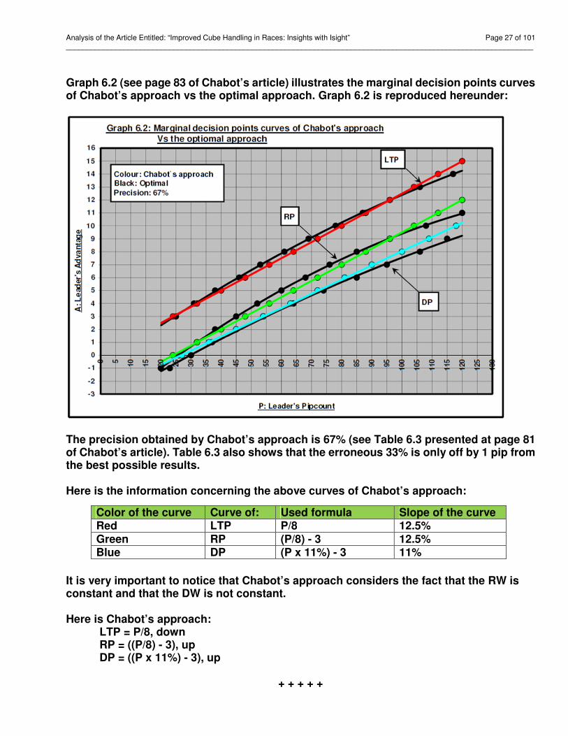
Graph 6.2 (see page 83 of Chabot’s article) illustrates the marginal decision points curves of Chabot’s approach vs the optimal approach. Graph 6.2 is reproduced hereunder:
The precision obtained by Chabot’s approach is 67% (see Table 6.3 presented at page 81 of Chabot’s article). Table 6.3 also shows that the erroneous 33% is only off by 1 pip from the best possible results. Here is the information concerning the above curves of Chabot’s approach: It is very important to notice that Chabot’s approach considers the fact that the RW is constant and that the DW is not constant. Here is Chabot’s approach:
LTP = P/8, down RP = ((P/8) - 3), up DP = ((P x 11%) - 3), up
+ + + + +
Color of the curve Curve of: Used formula Slope of the curve Red LTP P/8 12.5% Green RP (P/8) - 3 12.5% Blue DP (P x 11%) - 3 11%
Analysis of the Article Entitled: “Improved Cube Handling in Races: Insights with Isight” Page 28 of 101 _________________________________________________________________________________________________________________
2.5 Reichert’s comments concerning Chabot’s approach Regarding Chabot’s approach, on page 37 of his article, Reichert commented:
Chabot’s approach which is related to the “Gold standard table”, only approximates Trice Rule 62 (by using a denominator of 8, no shift for the point of last Take, and omitting the long/short race distinction).
The above excerpt contains two parts, namely:
• The first part: “Chabot’s approach which is related to the “Gold standard table”, only approximates Trice Rule 62”.
• The second part: “(by using a denominator of 8, no shift for the point of last Take, and omitting the long / short race distinction)”.
Before commenting on the first part, I will comment the second part.
• The LTP curve of Chabot’s approach has effectively a denominator of 8. Indeed, in section 2.4 of this article, we have seen that the LTP formula is: LTP = P/8. The slope is effectively 1/8, which corresponds to a slope of 12.5%. As illustrated in the graph entitled: “The Optimal-Chabot-Trice curves”, which is presented in section 2.6, the curve of Chabot practical (67%) almost perfectly matches the Optimal curve (100%). So, it necessarily implies that the best denominator is 8.
• The LTP curve of Chabot’s approach has effectively no shift for the point of last take. If we extrapolate Chabot’s LTP practical curve to P = 0 pip, we obtain A = 0 pip. So, there is no shift.
• The LTP theoretical curve of Chabot’s approach has effectively omitted the long/short race distinction. Indeed, the LTP curve of Chabot’s approach is a single straight line while the curve of Trice’s approach (or Trice Rule 62) is a combination of two straight lines (see section 2.3 of this article, see also the Graph entitled: The Optimal-Chabot-Trice curves, presented in section 2.6). So, Chabot’s approach effectively has no “long/short race distinction”.

Analysis of the Article Entitled: “Improved Cube Handling in Races: Insights with Isight” Page 29 of 101 _________________________________________________________________________________________________________________
Now, I will comment on the first part of the above excerpt, which is reproduced hereunder:
Chabot’s approach which is related to the “Gold standard table”, only approximates Trice Rule 62
In my opinion, the above excerpt could be interpreted in two different ways.
1) The first way to interpret this excerpt could be as follow: It is possible that Chabot's approach was obtained by using Trice's approach (i.e. Trice Rule 62) as a reference and approximating it.
2) The second way to interpret this excerpt could be as follow: It is possible that Chabot's approach was obtained without using Trice's approach (i.e. Trice Rule 62) as a reference and to realize that the obtained results for Chabot’s approach are very close to those obtained by Trice, so it could be said that Chabot’s approach only approximates Trice Rule 62.
To correctly interpret this extract, it is necessary to explain how Chabot’s article was developed. To begin, it may be necessary to inform the readers that around 1982, for my personal pleasure, I did computer work to assess the cubeless probability of winning (CPW) based on the pip count of each player. I obtained a table which was very similar to the table entitled “Probability of Winning the Race For the Player Who is on Roll” which is presented in Keith’s article entitled “Cube Handling In Noncontact Positions”. Unfortunately, I was not able to transform the obtained result into practical criteria to handle the cube. However, with a software like Snowie that can estimate with high accuracy the cubeless probability of winning as well as the proper cube action, I decided to continue the work I had already begun several years ago. To write Chabot’s article, which presents the optimal approach and Chabot’s approach, it has been necessary to find the right techniques that should be used in order to:
• Develop the optimal approach.
• Compare an approach to be analyzed with the optimal approach. • Evaluate the precision of an approach.
The required work was spread over a period of about 5 years. During this period:
• I analyzed all available information regarding cube handling in race for money games, so I had obviously analyzed Trice’s approach (or Trice Rule 62).
• I tried about 5 different techniques before finding the right techniques to: o Develop the optimal approach. o Compare an approach to be analyzed with the optimal approach. o Evaluate the precision of an approach.
• Snowie analyzed several hundreds of backgammon positions. Snowie probably worked for around 3,000 hours.
Analysis of the Article Entitled: “Improved Cube Handling in Races: Insights with Isight” Page 30 of 101 _________________________________________________________________________________________________________________
• I had even developed an approach much more precise than Trice’s. Indeed, I had developed an approach giving a precision of 91%. Given that it would have been too difficult to use, I considered that it was completely illogical to present a more accurate approach than Trice’s and end up not recommending it. So, in Chabot’s article, that approach was never presented.
To develop Chabot’s approach, I really did not try to “approximate Trice Rule 62”. I rather tried to obtain an approach giving the best possible precision using the optimal approach as a reference. Indeed, it should be noted that Graph 6.2 is entitled: “Marginal decision point curves of Chabot's approach vs the optimal approach”, not “Marginal decision point curves of Chabot's approach vs Trice’s approach”. In addition, when comparing graph 5.2 (see section 2.3) and graph 6.2 (see section 2.4), it is clear that the curves of Chabot's approach are quite different than Trice's. However for your information, here is the approach giving a precision of 91%:
When P is 62 pips or less DP = ((P/8) - 3.8), up RP = ((P/7) - 3.5), up LTP = ((P/7) - 0.5), down
When P is 63 pips or more
DP = ((P/10) - 2.4), up RP = ((P/10) - 0.6), up LTP = ((P/10) + 2.3), down
Given that I fully agree with Reichert that it is too complicated to use two “straight lines” (i.e. to use Trice’s practical approach which give a precision of 71%), it implies that the approach to use should only have one straight line and therefore it also implies that the precision obtained for the best practical approach will necessarily be under 71%. Given that the precision of Chabot’s approach is 67% and given that Chabot’s approach is very easy to remember and very easy to use; I do not believe that it will be possible to find a better practical approach. However, even if it is very unlikely that an easier and more precise approach than Chabot’s can be developed, it is nevertheless correct that Reichert tried to find a better practical approach.
+ + + + +
Analysis of the Article Entitled: “Improved Cube Handling in Races: Insights with Isight” Page 31 of 101 _________________________________________________________________________________________________________________
2.6 The Optimal-Chabot-Trice curves
The optimal approach has been presented in section 2.1 of this article. In summary, we have seen that:
• The optimal approach is the best theoretical approach presented so far. That approach is considered as being the reference. Therefore, the precision of that approach is defined as 100%.
• The RW (Redoubling Window) is pretty constant; indeed, the RW is about 3 pips.
• The DW (Doubling Window) is not constant. Indeed when P = 120 pips, the DW is about 5 pips and when P = 20 pips, the DW is about 3 pips.
Trice’s LTP theoretical curve has been presented in section 2.2 of this article. Trice has not presented any RP theoretical curve nor any DP theoretical curve. In summary, we have seen that:
• The precision obtained for Trice’s LTP theoretical curve is 75%. • Trice’s LTP theoretical curve corresponds almost exactly to the LTP
theoretical curve of the optimal approach.
• According to Reichert, Trice’s LTP theoretical values deserve to be termed “Gold standard table”. I agree with this terminology.
Trice’s practical approach has been presented in section 2.3 of this article. In summary, we have seen that:
• The precision obtained for Trice’s practical approach is 71%.
• According to Reichert, Trice’s criterion gives extremely accurate cube decisions. I also agree with this point of view.
• Chabot’s article do not recommend using this approach because it is too difficult to remember and too difficult to use.
• Reichert’s article also concluded that Trice’s approach with a “distinction between long and short race” requires too much effort to be used.
Chabot’s practical approach has been presented in section 2.4 of this article. In summary, we have seen that:
• The precision obtained for Chabot’s approach is 67%.
• The goal behind this approach was to obtain the best possible precision using the optimal approach as a reference.
• Chabot’s approach considers the fact that the RW is constant and that the DW is not constant.
• Reichert has correctly mentioned that the denominator of the LTP curve of Chabot’s approach is effectively 8.

Analysis of the Article Entitled: “Improved Cube Handling in Races: Insights with Isight” Page 32 of 101 _________________________________________________________________________________________________________________
The graph entitled “The Optimal-Chabot-Trice curves” which is hereunder presented, illustrates on the same graph the following four (4) curves:
1) The “Optimal (100%)” curve (the black curve), which is in fact the LTP theoretical curve of the optimal approach. This curve is presented in Section 2.1 of this article.
2) The “Trice theoretical (75%)” curve (the orange curve), which is in fact the LTP theoretical curve as presented by Trice. This curve is presented in section 2.2 of this article.
3) The “Trice practical (71%)” curve (the blue curve), which is in fact the LTP practical curve of Trice's approach. This curve is presented in Section 2.3 of this article.
4) The “Chabot practical (67%)” curve (the red curve), which is in fact the LTP practical curve of Chabot’s approach. This curve is presented in Section 2.4 of this article.
Notice that both theoretical curves (i.e. the black curve and the orange curve) are really “curves”, while both practical curves (i.e. the blue curve and the red curve) are “straight lines”.
0
1
2
3
4
5
6
7
8
9
10
11
12
13
14
15
16
17
18
19
0 5
10
15
20
25
30
35
40
45
50
55
60
65
70
75
80
85
90
95
100
105
110
115
120
125
130
A:
Lea
de
r's
Ad
va
nta
ge
P: Leader Pipcount
The Optimal-Chabot-Trice curves : LTP theoretical curve of the Optimal approach Vs LTP theoretical curve of Trice Vs LTP practical curve of Trice Vs LTP practical curve of Chabot
Optimal (100%)
Trice theoretical (75%)
Trice practical (71%)
Chabot practical (67%)
Analysis of the Article Entitled: “Improved Cube Handling in Races: Insights with Isight” Page 33 of 101 _________________________________________________________________________________________________________________
You should also notice that the curve of Chabot practical (67%) (i.e. the red curve) is a single straight line while the curve of Trice practical (71%) (i.e. the blue curve) is a combination of two straight lines. Namely, there is a straight line for the values below 62 pips and another for the values above 62 pips. In summary, the above graph clearly illustrates that:
• There is very little difference between these four curves.
• The curve of Chabot practical (67%) almost perfectly matches the optimal curve (100%).
Because there is very little difference between these four curves, we can conclude that each of these four curves give very accurate results.
+ + + + +
Analysis of the Article Entitled: “Improved Cube Handling in Races: Insights with Isight” Page 34 of 101 _________________________________________________________________________________________________________________
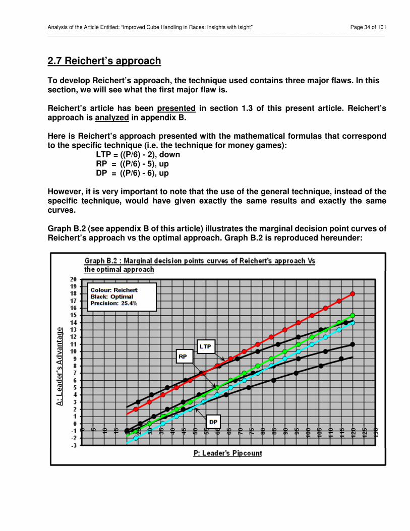
2.7 Reichert’s approach
To develop Reichert’s approach, the technique used contains three major flaws. In this section, we will see what the first major flaw is. Reichert’s article has been presented in section 1.3 of this present article. Reichert’s approach is analyzed in appendix B. Here is Reichert’s approach presented with the mathematical formulas that correspond to the specific technique (i.e. the technique for money games):
LTP = ((P/6) - 2), down RP = ((P/6) - 5), up DP = ((P/6) - 6), up
However, it is very important to note that the use of the general technique, instead of the specific technique, would have given exactly the same results and exactly the same curves. Graph B.2 (see appendix B of this article) illustrates the marginal decision point curves of Reichert’s approach vs the optimal approach. Graph B.2 is reproduced hereunder:
Analysis of the Article Entitled: “Improved Cube Handling in Races: Insights with Isight” Page 35 of 101 _________________________________________________________________________________________________________________
To develop his approach, Reichert employed a general framework. The general framework employed by Reichert is presented in Section 3 of Reichert's article. Here is this general framework:
• Concerning the LTP value, Reichert uses a “fraction” of the roller’s pip count and a “shift”.
• Concerning the RP value, Reichert uses a shift from the LTP values.
• Concerning the DP value, Reichert uses a shift from the LTP values.
It is very obvious that the LTP curve is the core of Reichert's approach. In section 2.1 of this article, we have seen that the RW is constant and that the shift from the LTP values is about 3 pips. We have also seen that the DW is not constant. Indeed, when P = 120 pips, the DW is about 5 pips and when P = 20 pips, the DW is about 3 pips.
In section 2.4 of this article, we have seen that according to Chabot’s approach, the DW is not constant.
To verify that the DW is not constant, it is very simple and the time needed is less than 5 minutes. You simply have to use Snowie and to proceed as follow:
1) Find any low-wastage position in which Black has exactly 120 pips. 2) Give exactly the same position to White. 3) Verify the cube action using: ‘’3-Ply Precise’’, you will obtain: No double, Take. 4) Move only 1 White checker until you obtain: Double, Take. At this pip count, you
have reached the DP (your Doubling point). White pip count should be around 129 pips, so your DP should be around 9 pips.
5) Continue to move the same White checker until you obtain: Double, Pass. At this pip count, you have reached the LTP (your Last Take Point). White pip count should be around 134 pips, so your LTP should be around 14 pips.
6) Since, the DW is obtained as follow: DW = LTP - DP; your DW should be around 5 pips.
7) Find any low-wastage position in which Black has exactly 70 pips and repeat exactly the same technique; the DW you obtain should be around 4 pips.
8) Find any low-wastage position in which Black has exactly 20 pips and repeat exactly the same technique; the DW you obtain should be around 3 pips.
Given that the general framework employed by Reichert considers that the DW is constant, it implies that the general framework used by Reichert has a major flaw. Indeed, it is the first major flaw committed by Reichert. The general framework employed by Reichert could have been fair before Chabot’s article was published. So, it is normal that theoreticians like Trice, Thorp, Keller, Keith and Ward have considered that the DW was constant. However, since Chabot’s article was published, using such general framework is definitively a major flaw.
Analysis of the Article Entitled: “Improved Cube Handling in Races: Insights with Isight” Page 36 of 101 _________________________________________________________________________________________________________________
Consequently, Reichert should definitively have considered that:
• The RW is constant.
• The DW is not constant. In fact, to use a similar metaphor used by Reichert, let’s suppose that there was a single needle in a haystack and that there is a person who want to find that needle. Then, the three options to consider are the following one:
1) First, this person is sure that the needle was not found. In this case it is normal that this person works to find that needle.
2) Second, this person does not know if the needle has actually already been found. In this case, this person could check if the needle has been found and based on the obtained answers, the person might decide to work to find that needle.
3) Third, this person is informed that the needle has actually been found. In this
case, this person should check if it is actually true. If after checking that it is indeed true, then it is obviously not necessary to continue to work to find another needle.
The option that corresponds to the whole situation concerning the DW is obviously the third option. Indeed, Reichert is perfectly informed that according to the optimal approach and to Chabot’s approach; the DW is not constant. So, it would have been perfectly normal for Reichert to check whether the DW is actually constant or not. Reichert should have verified if the results presented by the optimal approach, and by Chabot’s approach, were based or not. We have already seen that it is very easy to verify if the DW is constant or not and that it takes less than 5 minutes. In computer sciences, there is a jargon saying “Garbage in, garbage out” and it is exactly what Reichert did. Since the used hypotheses (i.e. the used general framework) are wrong, the obtained results are necessarily wrong. In summary, the general framework used by Reichert is wrong because he considered that the DW is constant. Consequently the obtained result, i.e. Reichert’s approach, is necessarily an unreliable approach.
+ + + + +

Analysis of the Article Entitled: “Improved Cube Handling in Races: Insights with Isight” Page 37 of 101 _________________________________________________________________________________________________________________
2.8 The Optimal-Chabot-Reichert curves
To develop Reichert’s approach, the technique used contains three major flaws. In this section, we will see what the second major flaw is. On page 37 of his article, Reichert has mentioned:
“WALTER TRICE came up with a table for money cube action in low-wastage positions. He was an expert in racing theory, so his table has been termed “gold standard table”. It contains the maximum pip deficit for the non-roller (point of last take) depending on the roller, pip count. The corresponding graph is plotted in figure 13.”
Here is this figure 13:
Figure 13: “Gold standard table” approximations with straight lines
Analysis of the Article Entitled: “Improved Cube Handling in Races: Insights with Isight” Page 38 of 101 _________________________________________________________________________________________________________________
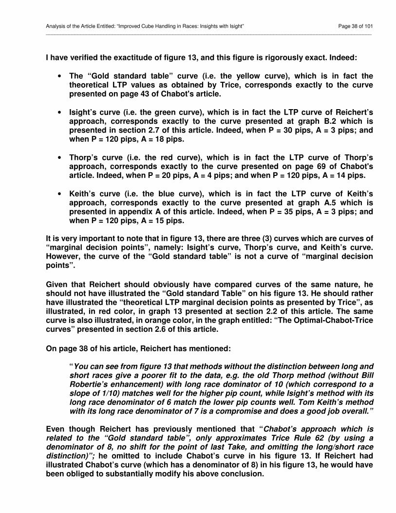
I have verified the exactitude of figure 13, and this figure is rigorously exact. Indeed:
• The “Gold standard table” curve (i.e. the yellow curve), which is in fact the theoretical LTP values as obtained by Trice, corresponds exactly to the curve presented on page 43 of Chabot's article.
• Isight’s curve (i.e. the green curve), which is in fact the LTP curve of Reichert’s approach, corresponds exactly to the curve presented at graph B.2 which is presented in section 2.7 of this article. Indeed, when P = 30 pips, A = 3 pips; and when P = 120 pips, A = 18 pips.
• Thorp’s curve (i.e. the red curve), which is in fact the LTP curve of Thorp’s approach, corresponds exactly to the curve presented on page 69 of Chabot's article. Indeed, when P = 20 pips, A = 4 pips; and when P = 120 pips, A = 14 pips.
• Keith’s curve (i.e. the blue curve), which is in fact the LTP curve of Keith’s approach, corresponds exactly to the curve presented at graph A.5 which is presented in appendix A of this article. Indeed, when P = 35 pips, A = 3 pips; and when P = 120 pips, A = 15 pips.
It is very important to note that in figure 13, there are three (3) curves which are curves of “marginal decision points”, namely: Isight’s curve, Thorp’s curve, and Keith’s curve. However, the curve of the “Gold standard table” is not a curve of “marginal decision points”.
Given that Reichert should obviously have compared curves of the same nature, he should not have illustrated the “Gold standard Table” on his figure 13. He should rather have illustrated the “theoretical LTP marginal decision points as presented by Trice”, as illustrated, in red color, in graph 13 presented at section 2.2 of this article. The same curve is also illustrated, in orange color, in the graph entitled: “The Optimal-Chabot-Trice curves” presented in section 2.6 of this article. On page 38 of his article, Reichert has mentioned:
“You can see from figure 13 that methods without the distinction between long and short races give a poorer fit to the data, e.g. the old Thorp method (without Bill Robertie’s enhancement) with long race dominator of 10 (which correspond to a slope of 1/10) matches well for the higher pip count, while Isight’s method with its long race denominator of 6 match the lower pip counts well. Tom Keith’s method with its long race denominator of 7 is a compromise and does a good job overall.”
Even though Reichert has previously mentioned that “Chabot’s approach which is related to the “Gold standard table”, only approximates Trice Rule 62 (by using a denominator of 8, no shift for the point of last Take, and omitting the long/short race distinction)”; he omitted to include Chabot’s curve in his figure 13. If Reichert had illustrated Chabot’s curve (which has a denominator of 8) in his figure 13, he would have been obliged to substantially modify his above conclusion.
Analysis of the Article Entitled: “Improved Cube Handling in Races: Insights with Isight” Page 39 of 101 _________________________________________________________________________________________________________________
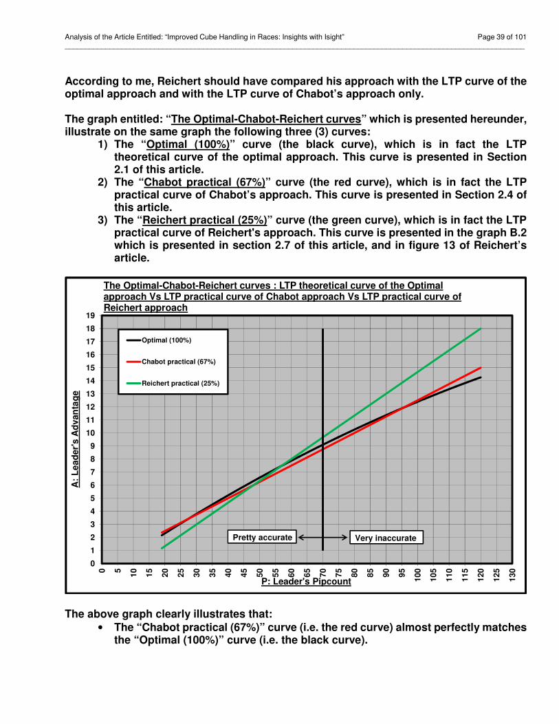
According to me, Reichert should have compared his approach with the LTP curve of the optimal approach and with the LTP curve of Chabot’s approach only. The graph entitled: “The Optimal-Chabot-Reichert curves” which is presented hereunder, illustrate on the same graph the following three (3) curves:
1) The “Optimal (100%)” curve (the black curve), which is in fact the LTP theoretical curve of the optimal approach. This curve is presented in Section 2.1 of this article.
2) The “Chabot practical (67%)” curve (the red curve), which is in fact the LTP practical curve of Chabot’s approach. This curve is presented in Section 2.4 of this article.
3) The “Reichert practical (25%)” curve (the green curve), which is in fact the LTP practical curve of Reichert's approach. This curve is presented in the graph B.2 which is presented in section 2.7 of this article, and in figure 13 of Reichert’s article.
The above graph clearly illustrates that:
• The “Chabot practical (67%)” curve (i.e. the red curve) almost perfectly matches the “Optimal (100%)” curve (i.e. the black curve).
0
1
2
3
4
5
6
7
8
9
10
11
12
13
14
15
16
17
18
19
0 5
10
15
20
25
30
35
40
45
50
55
60
65
70
75
80
85
90
95
10
0
10
5
11
0
11
5
12
0
12
5
13
0
A:
Le
ad
er'
s A
dvan
tag
e
P: Leader's Pipcount
The Optimal-Chabot-Reichert curves : LTP theoretical curve of the Optimal approach Vs LTP practical curve of Chabot approach Vs LTP practical curve of Reichert approach
Optimal (100%)
Chabot practical (67%)
Reichert practical (25%)
Pretty accurate Very inaccurate
Analysis of the Article Entitled: “Improved Cube Handling in Races: Insights with Isight” Page 40 of 101 _________________________________________________________________________________________________________________
• The “Reichert practical (25%)” curve (the green curve), which has a denominator of 6, does not match the “Optimal (100%)” curve (the black curve) at all; indeed the obtained results are pretty accurate for races shorter than 70 pips and very inaccurate for races above 70 pips.
Table B.3 (presented in appendix B) is used to calculate the precision of Reichert’s approach. This table also clearly shows that Reichert’s approach yields pretty good result only for races shorter than 70 pips. That’s why the precision obtained for Reichert’s approach is only 25%.
According to the graph above, when P = 100 pips:
• LTP = 12 pips with the optimal approach and with the Chabot’s approach;
• LTP = 14 pips with Reichert approach. The preceding results correspond perfectly with:
• Table 2.2 for the optimal approach (see page 53 of Chabot’s article). • Table 6.2 for Chabot’s approach (see page 80 of Chabot’s article).
• Table B.2 for Reichert’s approach (see appendix B of this article).
It is clear that the preceding result obtained using Reichert's approach is inaccurate. The use of an approach giving such inaccurate result would maybe have been appropriate 40 years ago. We are now in 2015, and all intermediate players should know that the correct answer is: LTP = 12 pips when P = 100 pips.
So, after realizing that his approach “is rather a poor fit of the gold standard table for higher pip counts”, Reichert answers the following question: “Why does Reichert’s approach perform so well in comparison with other approaches?” Given that Reichert has omitted to include Chabot’s approach in his figure 13, I do not know if Reichert considered Chabot’s approach as being included in the “other approaches” in the above statement. If Reichert had not omitted to include Chabot’s approach in his figure 13, Reichert might not have been able to conclude that his approach is the best approach proposed so far. His main argument is that it is “because most of the endgames are rather short”. He also argues that it is “better to adapt your heuristics to situation occurring frequently than rare cases”. Indeed, according to Reichert, the use of this technique “pays in terms of increased accuracy”. No matter the arguments (or answers) given by Reichert, the precision obtained for his approach (table B.3) will always remain 25%; and according to me, Reichert has to choose one of the three following options:
Analysis of the Article Entitled: “Improved Cube Handling in Races: Insights with Isight” Page 41 of 101 _________________________________________________________________________________________________________________
1) Option 1: To modify the database used in order to transform his unrepresentative database into a representative database (or into a very representative database). In this case, the obtained approach would be different and the obtained results (using the obtained approach) should be accurate for race length from 20 pips to 120 pips. Theoretically speaking, the obtained denominator (with a representative database) should be of 8 instead of 6. With this option, Reichert would certainly have to conclude that the obtained approach validates Trice Rule 62, the optimal approach and Chabot’s approach.
2) Option 2: To clearly mention that:
• The database used is a representative database only for races shorter than 70 pips; consequently, the obtained results are pretty accurate only for races shorter than 70 pips.
• The database used is a very unrepresentative database for races above 70 pips; consequently, the obtained results are very inaccurate for races above 70 pips.
• The database used is definitively a very unrepresentative database for the race length from 20 pips to 120 pips; consequently, the obtained approach can’t be used for race length from 20 pips to 120 pips.
• The obtained approach can’t be compared with Chabot’s approach, or any others approaches presented so far in which the race length is from 20 pips to 120 pips.
3) Option 3: To use a very unrepresentative database and to pretend that the
obtained approach is the best approach for race length from 20 pips to 120 pips, even if it is very obvious that the obtained result are pretty accurate only for races shorter than 70 pips and very inaccurate for long races.
Options 1 and 2 are both theoretically good but option 3 is obviously the only wrong theoretical option. According to me, Reichert should obviously have chosen option 1. Unfortunately, Reichert has chosen the option 3, which was the only wrong theoretical option. In page 20 (of his article) Reichert mentioned that he used Keith’s database. In pages 39 and 40 (of his article), Reichert presented in figure 14 the distribution of race length of Keith’s database and mentioned that:
• About 50% of the races are shorter than 40 pips
• About 90% of the races are shorter than 70 pips
• About 95% of the races are shorter than 75 pips
As clearly explained in appendix C entitled: “How to build a representative database”, a well weighed database, i.e. a representative database, should give the following results:
• 50% of the races are shorter than 70 pips
• 90% of the races are shorter than 110 pips • 95% of the races are shorter than 115 pips

Analysis of the Article Entitled: “Improved Cube Handling in Races: Insights with Isight” Page 42 of 101 _________________________________________________________________________________________________________________
In summary, a well weighed database should have 50% of all races shorter than 70 pips; while the Keith’s database as used by Reichert have about 90% of all races shorter than 70 pips.
So, it is very obvious that the database used by Reichert is actually a very unrepresentative database. Consequently, Reichert’s method is unreliable and the obtained results are inaccurate. Appendix C clearly explains how to proceed to transform an unrepresentative database into a representative database. The fact that Reichert used a very unrepresentative database and pretended that the obtained approach is reliable from 20 pips to 120 pips is obviously a major flaw. Indeed, it is Reichert’s second major flaw. Reichert also answers his own following question: “Could Reichert’s approach be improved even further?” He said that it would be possible by using 3 additional parameters and a new formula, but according to him it is not worth the effort. Here is my answer:
• It is obvious that Reichert might further improve his approach by simply assuming that the DW is not constant and by using a representative database instead of an unrepresentative database.
• I am convinced that if Reichert had considered that the DW is not constant and if he had modified his unrepresentative database to obtain a representative database; then, he would have certainly obtained an approach in which the denominator for the LTP curve is 8 (instead of 6), and he would also certainly have obtained an approach having criteria similar to those of Chabot’s approach.
+ + + + +
Analysis of the Article Entitled: “Improved Cube Handling in Races: Insights with Isight” Page 43 of 101 _________________________________________________________________________________________________________________
2.9 Reichert’s refusal to verify the accuracy of the optimal approach To develop Reichert’s approach, the technique used contains three major flaws. In this section, we will see what the third major flaw is. Before publishing this article, I exchanged several email with Reichert. Indeed, I tried to convince him that the best theoretical approach proposed so far is the optimal approach; and that the best practical approach proposed so far is Chabot’s approach. I also tried to perfectly understand his viewpoint regarding the fact that, according to me, his approach contains two major flaws and that it is the worst approach proposed so far. It is necessary to mention that before I exchanged email with Reichert, I thought that to develop his approach, the technique used contained “only” two major flaws. After the email exchange, I was rather convinced that a third major flaw was involved to develop his approach. That third flaw is related to the objective of his optimization. Indeed, his objective was incorrectly chosen. In the first three (3) emails I send to Reichert, I clearly explained to him that, according to me, his approach contained two major flaws, namely:
• The technique used considers that the DW (Doubling Window) is constant, while the DW is not constant.
• The database used is a very unrepresentative database, while this database should have been a representative database.
I also clearly explained to him that, according to me, the combination of these two major flaws results in his decision criteria being unreliable and inaccurate. I also sent him the calculation regarding the precision of his approach being only 25%. In my fourth and subsequent emails, I asked Reichert several questions and he asked me several questions back.
+ + + + + Here is a question I asked Reichert:
To develop the Isight method, did you verify if the DW (Doubling Window) is constant or not constant?
Reichert answered that, according to him, it was not relevant to verify this point. He also very clearly answered that before he developed the Isight method, he did not verify it.
+ + + + +
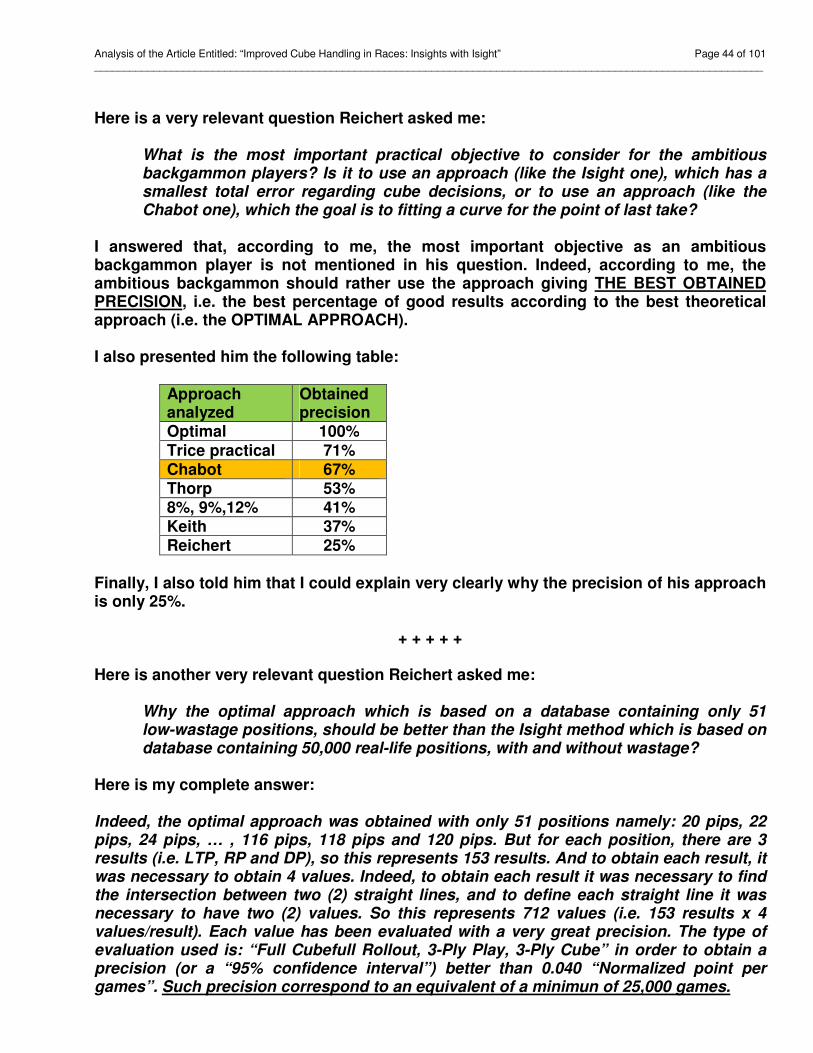
Analysis of the Article Entitled: “Improved Cube Handling in Races: Insights with Isight” Page 44 of 101 _________________________________________________________________________________________________________________
Here is a very relevant question Reichert asked me: What is the most important practical objective to consider for the ambitious backgammon players? Is it to use an approach (like the Isight one), which has a smallest total error regarding cube decisions, or to use an approach (like the Chabot one), which the goal is to fitting a curve for the point of last take?
I answered that, according to me, the most important objective as an ambitious backgammon player is not mentioned in his question. Indeed, according to me, the ambitious backgammon should rather use the approach giving THE BEST OBTAINED PRECISION, i.e. the best percentage of good results according to the best theoretical approach (i.e. the OPTIMAL APPROACH). I also presented him the following table:
Approach analyzed
Obtained precision
Optimal 100% Trice practical 71% Chabot 67% Thorp 53% 8%, 9%,12% 41% Keith 37% Reichert 25%
Finally, I also told him that I could explain very clearly why the precision of his approach is only 25%.
+ + + + + Here is another very relevant question Reichert asked me:
Why the optimal approach which is based on a database containing only 51 low-wastage positions, should be better than the Isight method which is based on database containing 50,000 real-life positions, with and without wastage?
Here is my complete answer: Indeed, the optimal approach was obtained with only 51 positions namely: 20 pips, 22 pips, 24 pips, … , 116 pips, 118 pips and 120 pips. But for each position, there are 3 results (i.e. LTP, RP and DP), so this represents 153 results. And to obtain each result, it was necessary to obtain 4 values. Indeed, to obtain each result it was necessary to find the intersection between two (2) straight lines, and to define each straight line it was necessary to have two (2) values. So this represents 712 values (i.e. 153 results x 4 values/result). Each value has been evaluated with a very great precision. The type of evaluation used is: “Full Cubefull Rollout, 3-Ply Play, 3-Ply Cube” in order to obtain a precision (or a “95% confidence interval”) better than 0.040 “Normalized point per games”. Such precision correspond to an equivalent of a minimun of 25,000 games.
Analysis of the Article Entitled: “Improved Cube Handling in Races: Insights with Isight” Page 45 of 101 _________________________________________________________________________________________________________________
So, the optimal approach has been obtained with 712 very representative values. According to me, this is enough to obtain very reliable and very accurate results. Here is an extract from page 4 of my article:
‘’Part 1 entitled: "The optimal approach", begins by giving the definitions and explanations of all the concepts that will be used in this article. This first part also presents in great detail, the technique used to develop the optimal approach. This part was written to allow a skeptical reader to be able to verify this technique, and to be able to confirm that the obtained approach is really the optimal one.’’
Note: The underlined has been added Here is the last paragraph of section 1.5 of my article:
‘’If you ever decide to perform the exact same exercise, your results could obviously be very slightly different, because your positions would necessarily be different from those that were in fact used to carry out this analysis. But, you can be sure that all the results you get will be very similar to those illustrated in graph 3.’’
According to me, any skeptical reader should be able to verify the technique used to develop the optimal approach. So, it should be very easy for you to really check the validity of the optimal approach.
So, to obtain the best possible answer to your above question, I simply propose you the following challenge:
1) Make the needed exercise and compare the results you obtain with the presented results (i.e. graph 3 and graph 10).
2) If you do not wish to accept the proposed challenge, you may ask any backgammon player (you know) to do the needed exercise.
As illustrated on graph 13 (see page 45 of my article), the LTP curve of the optimal approach and the LTP curve of the ‘’Gold standard table’’ almost perfectly fit together. Consequently, I am very confident that you will also obtain very similar results. I am also very confident that any skeptical reader will also obtain very similar results. I am 100% convinced that you should have done this exercise before writing your article, not after; but better late than never. Once you obtain the results of the proposed challenge, then you will have the ONLY correct answer to your own above question, i.e. the best theoretical approach proposed so far, is really the OPTIMAL APPROACH.

Analysis of the Article Entitled: “Improved Cube Handling in Races: Insights with Isight” Page 46 of 101 _________________________________________________________________________________________________________________
To use 50,000 real-life positions, with and without wastage, does not mean that the obtained database containing these positions is well weighed. As I have already explained to you, I think that your database is poorly weighted to represent the big picture. As you mentioned yourself, short races (< 70pips) occurs more frequently than long races (>70pips) so, of course, your approach has a closer fit for short races. This also has the effect of representing poorly the long races that occur less often. You can't claim to have the best decision criteria for races from 20 pips to 120 pips because you database is too weighted heavily for races shorter than 70 pips. Referring to the figure 14 of your article (Race length and positions), you mention that about 90% of your database is races shorter than 70 pips, while a well weighed database should have 50% of races shorter than 70 pips. As I have already explained to you, I believe a well weighted database should have the same number of positions represented at every race length. In summary the database used to obtain the optimal approach is a very representative database because the 712 values are very precise and very well weighted; while your database is unrepresentative because your 50,000 real-life positions are not very well weighted. Your database is certainly a very good database, but it is not a representative database. To obtain a representative database, it is necessary to make transformations. I could explain you how to make these transformations. Once you give me your results from the proposed challenge I will be pleased to answer any other questions.
+ + + + + IT SHOULD BE NOTED THAT REICHERT DID NOT ACCEPT MY CHALLENGE TO VERIFY THE ACCURACY OF THE OPTIMAL APPROACH AND THAT HE HAS NOT EVEN GIVEN ANY COMMENT REGARDING HIS REFUSAL.
+ + + + + Here is a question I asked Reichert:
According the Isight method, when the leader’s adjusted pip count is 100 pips, the LTP to use is 14 pips. So, do you seriously recommend that LTP should be 14 pips when the leader’s adjusted pip count is 100 pips? If yes, would you accept to play such position as money proposition?
Reichert answered that even if the obtained answer according the Isight method is LTP = 14 pips, he would rather use LTP = 12 pips to play a money proposition.
+ + + + +

Analysis of the Article Entitled: “Improved Cube Handling in Races: Insights with Isight” Page 47 of 101 _________________________________________________________________________________________________________________
To make sure I perfectly understood the preceding answer, I sent Reichert the following email:
Hi Axel There is theory, and there is also practice. When the adjusted leader’s pip count is 100 pips:
• In theory, we have:
Reference LTP value Optimal approach 12 pips Trice (or ‘’Gold standard table’’) 12 pips
• However, in practice, we have:
Reference Practical decision criteria to use (P = 100 pips)
Obtained LTP value
Trice practical ((P/10) +1), up 11 pips Chabot P/8, down 12 pips Thorp ((P x 10%) +2), down 12 pips 8%, 9%,12% (P x 12%), down 12 pips Keith ((P/7) - 2), down 12 pips Isight ((P/6) - 2), down 14 pips
Question no 1:
Do you agree, yes or no, that the theoritical LTP’s value is 12 pips?
Question no 2:
Do you agree, yes or no, that all the above practical decision criteria to use, are the correct one?
Question no 3:
Do you agree, yes or no, that all the obtained LTP value, are well calculated? Once you will have clearly answered to these three (3) above questions, I will obviously have several other questions to ask you. Best regards Michelin
+ + + + +
Analysis of the Article Entitled: “Improved Cube Handling in Races: Insights with Isight” Page 48 of 101 _________________________________________________________________________________________________________________
In his reply, Reichert did not answer any of my three (3) very specific questions, he rather gave me very irrelevant answers and he concluded as follow: “I will not spend further time on trying to convince you.” So, because he has clearly refused to answer my last email and because of the content of his last reply; I decided to stop exchanging with him.
+ + + + +
The most relevant points of the “discussion” (or email exchange) with Reichert, could be summarized as follow:
1) Chabot’s article explains in great detail the technique used to develop the OPTIMAL APPROACH. The technique used was presented in a very detailed way to allow any skeptical reader to verify this technique and to confirm that the obtained approach is really the optimal one. To prove Reichert that the best theoretical approach proposed so far is the OPTIMAL APPROACH; I challenged him to verify himself the accuracy of this approach.
Even if Reichert should have checked the accuracy of the OPTIMAL APPROACH before writing his article; he should have accepted the preceding challenge; indeed, better late than never; but, REICHERT HAS REFUSED MY CHALLENGE WITHOUT EVEN GIVING ANY EXPLANATION.
2) According to the optimal approach, the DW is not constant. In order to verify that
the DW is effectively not constant, the needed time is less than 5 minutes. Reichert should have verified if the DW is constant or not constant. To develop his approach, Reichert incorrectly used the hypothesis that the DW is constant. According to Reichert, the fact that the DW is constant or not constant is not relevant, and consequently he has not verified this point.
3) According to me, to determine what the best practical approach is, the objective is to find the approach giving the best precision (i.e. the best percentage of good results), in relation to the best theoretical approach (i.e. the OPTIMAL APPROACH). According to Reichert, to determine what the best practical approach is, the objective is to find the approach giving the “smallest total error regarding cube decisions”, in relation to a “database containing about 50,000 real-life positions, with and without wastage”.
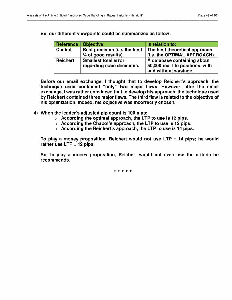
Analysis of the Article Entitled: “Improved Cube Handling in Races: Insights with Isight” Page 49 of 101 _________________________________________________________________________________________________________________
So, our different viewpoints could be summarized as follow:
Reference Objective In relation to: Chabot Best precision (i.e. the best
% of good results). The best theoretical approach (i.e. the OPTIMAL APPROACH).
Reichert Smallest total error regarding cube decisions.
A database containing about 50,000 real-life positions, with and without wastage.
Before our email exchange, I thought that to develop Reichert’s approach, the technique used contained “only” two major flaws. However, after the email exchange, I was rather convinced that to develop his approach, the technique used by Reichert contained three major flaws. The third flaw is related to the objective of his optimization. Indeed, his objective was incorrectly chosen.
4) When the leader’s adjusted pip count is 100 pips: o According the optimal approach, the LTP to use is 12 pips. o According the Chabot’s approach, the LTP to use is 12 pips. o According the Reichert’s approach, the LTP to use is 14 pips.
To play a money proposition, Reichert would not use LTP = 14 pips; he would rather use LTP = 12 pips. So, to play a money proposition, Reichert would not even use the criteria he recommends.
+ + + + +

Analysis of the Article Entitled: “Improved Cube Handling in Races: Insights with Isight” Page 50 of 101 _________________________________________________________________________________________________________________
2.10 Precision of Reichert’s approach The best way to compare the accuracy of Reichert’s approach with other approaches is not to compare Reichert’s approach LTP curve with other LTP curves; it is rather to calculate its precision and to compare it with the precision of other approaches. The only way to calculate the precision of an approach is clearly explained in the section 2.1 of the Chabot’s article (see page 50 of the Chabot’s article). Table B.3 shows the calculation of Reichert’s approach precision. The obtained results are:
• Good results……………………..... 25.4%
• Results with a 1-pip difference…. 38.3% • Results with a 2-pip difference…. 14.9%
• Results with a 3-pip difference…. 12.9% • Results with a 4-pip difference…. 8.3%
• Results with a 5-pip difference…. 0.3% So, the precision (i.e. the percentage of good results) of Reichert’s approach is only 25%. Here is the comparison of Reichert’s approach precision with other approaches:
Approach analyzed
Obtained precision
Reference
Optimal 100% Page 51 of Chabot’s article Trice practical 71% Page 74 of Chabot’s article Chabot 67% Page 81 of Chabot’s article Thorp 53% Page 67 of Chabot’s article 8%, 9%,12% 41% Page 60 of Chabot’s article Keith 37% Appendix A of this article Reichert 25% Appendix B of this article
As clearly shown in the above table, Reichert’s approach has the worst precision so far. Even the “very old” 8%, 9%, 12% approach is more precise than Reichert’s approach.
+ + + + +

Analysis of the Article Entitled: “Improved Cube Handling in Races: Insights with Isight” Page 51 of 101 _________________________________________________________________________________________________________________
2.11 Financial results: Reichert’s approach vs Chabot’s approach
The goal of this section is to compare Chabot’s approach with Reichert’s approach in order to deduce what approach should give the best expected financial results. According to me, THE BEST way to verify if Chabot’s approach is better than Reichert’s approach is to COMPARE THE EXPECTED FINANCIAL RESULTS OF EACH APPROACH. I am sure that Reichert would agree with this preceding statement. When Reichert was willing to exchange email with me, my goal was to slowly elaborate, step by step, the content of appendix D which is entitled: “Theoretical Money Proposition”. Even if I perfectly knew the conclusion of that appendix, I nevertheless expected to be able to explain him, step by step, how to build it. However, when I received Reichert’s last email, he clearly refused to answer my questions and he would certainly refuse to answer my next questions. Since he clearly told me “I will not spend further time on trying to convince you” in his last email, I decided not to send him email anymore. Consequently, I was never able to explain him the content of Appendix D. Chabot’s approach and Reichert’s approach are both practical decision criteria for race length from 20 pips to 120 pips i.e. 101 pips. Since there are 3 results for each race length, (i.e. LTP, RP and DP), there is a total of 303 results. So, Chabot’s approach and Reichert’s approach are simply three tables (of 101 values per table) giving 303 results. Indeed, the 303 results of Chabot’s approach are presented in section 1.2 of this article; while the 303 results of Reichert’s approach are presented in section 1.3 of this article. I am sure that Reichert should agree with that statement, but I am not sure if Reichert would effectively agree with that statement. According to me, the approach giving the best precision, i.e. the greater number of good results, is necessarily the best approach. To evaluate if a result is good or not, according to me, the best way is to use the best theoretical approach as a reference, i.e. the OPTIMAL APPROACH. Therefore, I calculated the precision of each approach. The precision obtained for Chabot’s approach is 67% (See Appendix D, see also the Table 6.3 presented at page 81 of Chabot’s article) and the precision obtained for Reichert’s approach is ONLY 25% (See Appendix D, see also Table B.3 presented at Appendix B of this article). I am sure that Reichert would not agree with me regarding this statement. According to me, to evaluate the accuracy of an approach and therefore, the expected financial results, it is also possible to play several theoretical money propositions. I believe that Reichert would agree that such technique should give accurate result, but I am not sure. I would have liked to elaborate this specific point with him but, as I have already explained, I decided not to send him email anymore.

Analysis of the Article Entitled: “Improved Cube Handling in Races: Insights with Isight” Page 52 of 101 _________________________________________________________________________________________________________________
For example, when the leader’s adjusted pip count is 100 pips:
• According to the optimal approach, the LTP to use is 12 pips.
• According the Chabot’s approach, the LTP to use is 12 pips. • According the Reichert’s approach, the LTP to use is 14 pips.
If this specific position was played as a theoretical money proposition, according to me, the obtained result should correspond to the obtained results of the OPTIMAL APPROACH; and consequently the winner of this specific theoretical money proposition should be Chabot’s approach. I am not sure if Reichert would agree with me regarding this statement. Even if Reichert clearly mentioned that the decision criteria of the Isight method poorly matches the “Gold standard table” for long race and even if Reichert has clearly told me that he would rather use LTP = 12 pips instead of LTP = 14 pips to play this preceding theoretical money proposition; I have to repeat that I am not sure if Reichert would agree with me that the winner of this specific theoretical money proposition should be Chabot’s approach. According to me, it is very obvious; but I really do not know if Reichert would agree or disagree with me regarding this specific statement. The expected results for the 303 possible theoretical money propositions are presented in appendix D. Among these 303 results, according to Appendix D, there are 81 positions in which Reichert’s approach and Chabot’s approach have the same results (i.e. the same gap with regard to the optimal approach). So, for these specific positions, it is not relevant to play a theoretical money proposition. I am sure that Reichert would agree with me about this. In appendix D, there are 222 positions (i.e. 303 positions – 81 positions) in which Reichert’s approach and Chabot’s approach does not have the same result. In these positions, according to me, the winner of each theoretical money proposition is the approach with which the result is the closest to the result of the OPTIMAL APPROACH. I am sure that Reichert would disagree with me regarding this point. As shown in appendix D, the results of Chabot’s approach are:
The worst error is ONLY 1 pip. As shown in appendix D, the results of Reichert’s approach are:
Good results 204 on 303 = 67.3% Results with a 1-pip difference 99 on 303 = 32.7%
Good results 77 on 303 = 25.4% Results with a 1-pip difference 116 on 303 = 38.3% Results with a 2-pip difference 45 on 303 = 14.9% Results with a 3-pip difference 39 on 303 = 12.9% Results with a 4-pip difference 25 on 303 = 8.3% Results with a 5-pip difference 1 on 303 = 0.3%

Analysis of the Article Entitled: “Improved Cube Handling in Races: Insights with Isight” Page 53 of 101 _________________________________________________________________________________________________________________
The worst error of Reichert’s approach is 5 pips. This specific error is obtained when the Leader’s pip count is 115 pips. Indeed, according to the optimal approach, the DP (Doubling Point) is 9 pips, while according to Reichert’s approach the DP is 14 pips. As shown in Appendix D, the results of the theoretical money propositions are:
Description Results Reichert’s approach and Chabot’s approach have exactly the same result (i.e. the same gap with regard to the optimal approach). So, it is irrelevant to play a theoretical money proposition.
81 positions
Chabot’s approach should win the theoretical money proposition.
197 positions
Reichert’s approach should win the theoretical money proposition.
25 positions
Total 303 positions The expected result of the theoretical money proposition, are:
• Among the 303 results, there is no winner for 81 results and there is a winner for 222 results.
• Among these 222 results in which there is a winner, Chabot’s approach win 89% of these results (i.e. 197/222).
• Among these 222 results in which there is a winner, Reichert’s approach win ONLY 11% of these results (i.e. 25/222).
Therefore, Chabot’s approach definitively gives better financial results than Reichert’s approach. I am sure that Reichert would necessarily disagree with me regarding this point and, unfortunately, I really do not know how to convince Reichert that the 303 values for Chabot’s approach are more accurate than the 303 values for Reichert’s approach.
To prove Reichert that Chabot’s approach is better than his approach; it is necessary to know what he thinks about Appendix D. It would be very interesting if Reichert presented an appendix similar to Appendix D, i.e. a clear table which contains Reichert’s expected financial results for each possible 303 values. Consequently, I challenge Reichert to present an Appendix similar to my Appendix D. This is challenge number 1. For each of the 197 positions in which, according the Appendix D, Chabot’s approach should win, it would be interesting to know if Reichert would agree that Chabot’s approach should win. It would also be interesting to know if Reichert would accept to play a theoretical money proposition (or a real money proposition) for each of these 197 positions. Consequently, I challenge Reichert to clearly mention if he would accept to play a theoretical money proposition (or a real money proposition) for each of these 197 positions. This is challenge number 2.
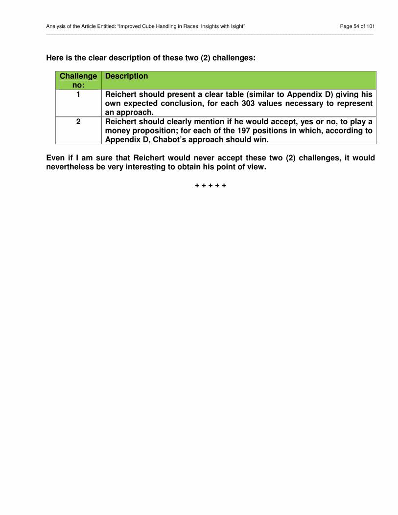
Analysis of the Article Entitled: “Improved Cube Handling in Races: Insights with Isight” Page 54 of 101 _________________________________________________________________________________________________________________
Here is the clear description of these two (2) challenges:
Challenge no:
Description
1 Reichert should present a clear table (similar to Appendix D) giving his own expected conclusion, for each 303 values necessary to represent an approach.
2 Reichert should clearly mention if he would accept, yes or no, to play a money proposition; for each of the 197 positions in which, according to Appendix D, Chabot’s approach should win.
Even if I am sure that Reichert would never accept these two (2) challenges, it would nevertheless be very interesting to obtain his point of view.
+ + + + +
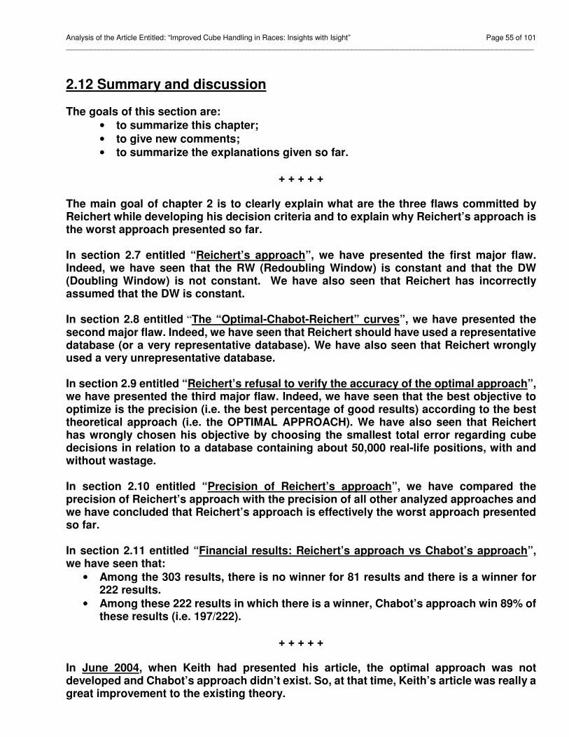
Analysis of the Article Entitled: “Improved Cube Handling in Races: Insights with Isight” Page 55 of 101 _________________________________________________________________________________________________________________
2.12 Summary and discussion
The goals of this section are: • to summarize this chapter;
• to give new comments; • to summarize the explanations given so far.
+ + + + +
The main goal of chapter 2 is to clearly explain what are the three flaws committed by Reichert while developing his decision criteria and to explain why Reichert’s approach is the worst approach presented so far. In section 2.7 entitled “Reichert’s approach”, we have presented the first major flaw. Indeed, we have seen that the RW (Redoubling Window) is constant and that the DW (Doubling Window) is not constant. We have also seen that Reichert has incorrectly assumed that the DW is constant. In section 2.8 entitled “The “Optimal-Chabot-Reichert” curves”, we have presented the second major flaw. Indeed, we have seen that Reichert should have used a representative database (or a very representative database). We have also seen that Reichert wrongly used a very unrepresentative database. In section 2.9 entitled “Reichert’s refusal to verify the accuracy of the optimal approach”, we have presented the third major flaw. Indeed, we have seen that the best objective to optimize is the precision (i.e. the best percentage of good results) according to the best theoretical approach (i.e. the OPTIMAL APPROACH). We have also seen that Reichert has wrongly chosen his objective by choosing the smallest total error regarding cube decisions in relation to a database containing about 50,000 real-life positions, with and without wastage. In section 2.10 entitled “Precision of Reichert’s approach”, we have compared the precision of Reichert’s approach with the precision of all other analyzed approaches and we have concluded that Reichert’s approach is effectively the worst approach presented so far. In section 2.11 entitled “Financial results: Reichert’s approach vs Chabot’s approach”, we have seen that:
• Among the 303 results, there is no winner for 81 results and there is a winner for 222 results.
• Among these 222 results in which there is a winner, Chabot’s approach win 89% of these results (i.e. 197/222).
+ + + + +
In June 2004, when Keith had presented his article, the optimal approach was not developed and Chabot’s approach didn’t exist. So, at that time, Keith’s article was really a great improvement to the existing theory.

Analysis of the Article Entitled: “Improved Cube Handling in Races: Insights with Isight” Page 56 of 101 _________________________________________________________________________________________________________________
In May 2014, I published an article entitled “Money Cube Action in Low-wastage Positions”. That article presents a theoretical approach that is called the optimal approach and a practical approach that is called Chabot's approach. Here is the summary of Chabot’s article:
• The database used to obtain the optimal approach was a very representative database.
• The optimal approach clearly illustrates that: o The RW is constant. o The DW is not constant. Indeed when P = 120 pips, the DW is about 5 pips;
and when P = 20 pips, the DW is about 3 pips.
• Chabot’s approach considers that the RW is constant and that the DW is not constant. Indeed, Chabot’s approach is as follow: o LTP = P/8, down o RP = ((P/8) - 3), up o DP = ((P x 11%) - 3), up
• Trice’s approach is more precise than Chabot’s approach, indeed: o The precision obtained for Trice’s approach is 71%. o The precision obtained for Chabot’s approach is 67%.
• Trice’s approach was not recommended because it is too difficult to memorize and too difficult to use.
In June 2014, Reichert presented his article. Here is my summary of Reichert’s article regarding Reichert’s approach:
• The general framework used to obtain Reichert’s approach considers that the DW is constant.
• The database used to obtain Reichert’s approach was a good but very unrepresentative database.
• The specific Reichert approach is as follow: o LTP = ((P/6) - 2), down o RP = ((P/6) - 5), up o DP = ((P/6) - 6), up
• Reichert’s approach is the best approach proposed so far (according to him
and the worst according to me).
+ + + + +
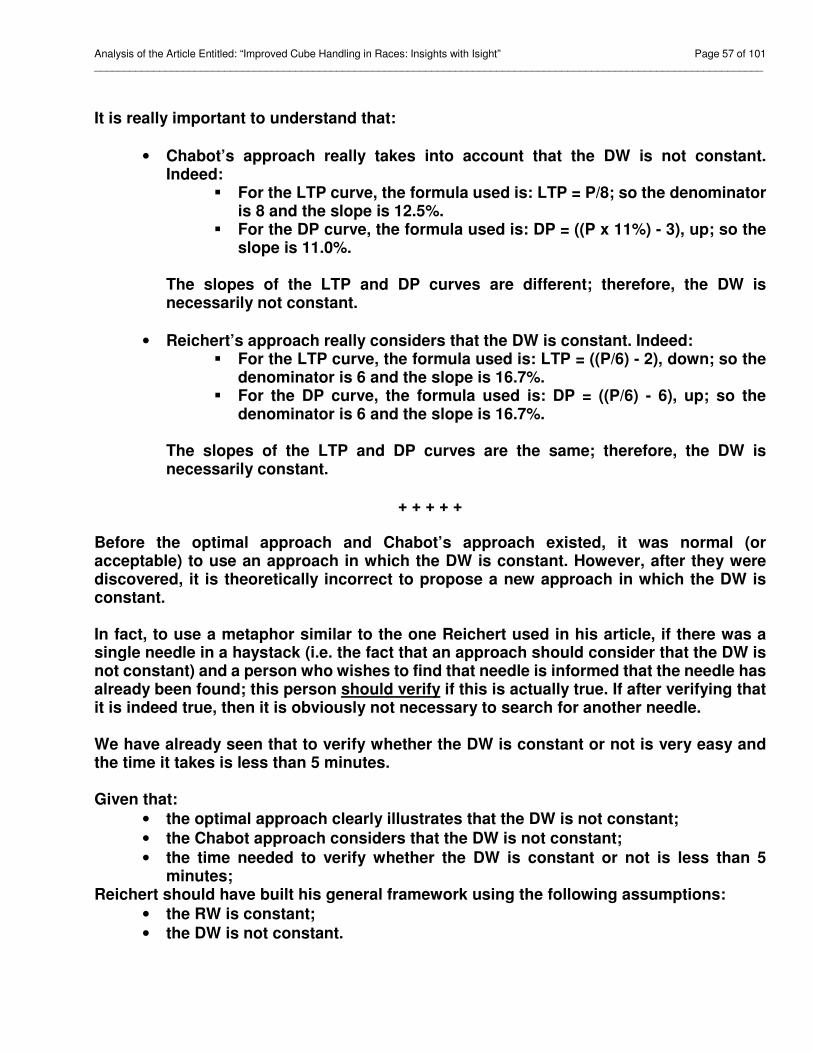
Analysis of the Article Entitled: “Improved Cube Handling in Races: Insights with Isight” Page 57 of 101 _________________________________________________________________________________________________________________
It is really important to understand that:
• Chabot’s approach really takes into account that the DW is not constant. Indeed:
� For the LTP curve, the formula used is: LTP = P/8; so the denominator is 8 and the slope is 12.5%.
� For the DP curve, the formula used is: DP = ((P x 11%) - 3), up; so the slope is 11.0%.
The slopes of the LTP and DP curves are different; therefore, the DW is necessarily not constant.
• Reichert’s approach really considers that the DW is constant. Indeed: � For the LTP curve, the formula used is: LTP = ((P/6) - 2), down; so the
denominator is 6 and the slope is 16.7%. � For the DP curve, the formula used is: DP = ((P/6) - 6), up; so the
denominator is 6 and the slope is 16.7%.
The slopes of the LTP and DP curves are the same; therefore, the DW is necessarily constant.
+ + + + +
Before the optimal approach and Chabot’s approach existed, it was normal (or acceptable) to use an approach in which the DW is constant. However, after they were discovered, it is theoretically incorrect to propose a new approach in which the DW is constant. In fact, to use a metaphor similar to the one Reichert used in his article, if there was a single needle in a haystack (i.e. the fact that an approach should consider that the DW is not constant) and a person who wishes to find that needle is informed that the needle has already been found; this person should verify if this is actually true. If after verifying that it is indeed true, then it is obviously not necessary to search for another needle. We have already seen that to verify whether the DW is constant or not is very easy and the time it takes is less than 5 minutes. Given that:
• the optimal approach clearly illustrates that the DW is not constant; • the Chabot approach considers that the DW is not constant;
• the time needed to verify whether the DW is constant or not is less than 5 minutes;
Reichert should have built his general framework using the following assumptions:
• the RW is constant; • the DW is not constant.

Analysis of the Article Entitled: “Improved Cube Handling in Races: Insights with Isight” Page 58 of 101 _________________________________________________________________________________________________________________
The fact that Reichert designed his “general framework” and his own approach with the assumption that the DW is constant is obviously a major flaw. Indeed, this is the first major flaw committed by Reichert. In computer sciences, there is a jargon saying “Garbage in, garbage out”. It is exactly what Reichert did. Since the used hypotheses are wrong, the obtained results are necessarily wrong. Reichert’s approach is necessarily unreliable and inaccurate because he considered that the DW is constant. This concludes the discussion regarding the first flaw. Now, let’s analyze the second flaw.
+ + + + + The graph entitled “The Optimal-Chabot-Trice curves” and the graph entitled “The Optimal-Chabot-Reichert curves” are hereunder presented:
The Optimal-Chabot-Trice curves clearly illustrate that:
• The “Chabot practical (67%)” curve (the red curve in both graph), which has a denominator of 8, almost perfectly matches the “Optimal (100%)” curve (the black curve in both graph);
• The “Trice theoretical (75%)” curve (the orange curve), which correspond to the “Gold standard table”, almost perfectly matches the “Optimal (100%)” curve (the black curve in both graph);
• The “Trice practical (71%)” curve (the blue curve), which according to Reichert, gives extremely accurate handling cube action, almost perfectly matches the “Optimal (100%)” curve (the black curve in both graph);
The graph entitled “The Optimal-Chabot-Reichert curves” clearly illustrates that:
• The “Chabot practical (67%)” curve (the red curve in both graph), which has a denominator of 8, almost perfectly marches the “Optimal (100%)” curve (the black curve in both graph);
0
1
2
3
4
5
6
7
8
9
10
11
12
13
14
15
16
17
18
19
0 5
10
15
20
25
30
35
40
45
50
55
60
65
70
75
80
85
90
95
10
0
10
5
11
0
11
5
12
0
12
5
13
0
A:
Le
ad
er'
s A
dv
an
tag
e
P: Leader Pipcount
The Optimal-Chabot-Trice curves : LTP theoretical curve of the Optimal approach Vs LTP theoretical curve of Trice Vs LTP practical curve of Trice Vs LTP practical curve of Chabot
Optimal (100%)
Trice theoretical (75%)
Trice practical (71%)
Chabot practical (67%)
0
1
2
3
4
5
6
7
8
9
10
11
12
13
14
15
16
17
18
19
0 5
10
15
20
25
30
35
40
45
50
55
60
65
70
75
80
85
90
95
100
105
110
115
120
125
130
A:
Le
ad
er'
s A
dva
nta
ge
P: Leader's Pipcount
The Optimal-Chabot-Reichert curves : LTP theoretical curve of the Optimal approach Vs LTP practical curve of Chabot approach Vs LTP practical curve of Reichert approach
Optimal (100%)
Chabot practical (67%)
Reichert practical (25%)
Pretty accurate Very inaccurate
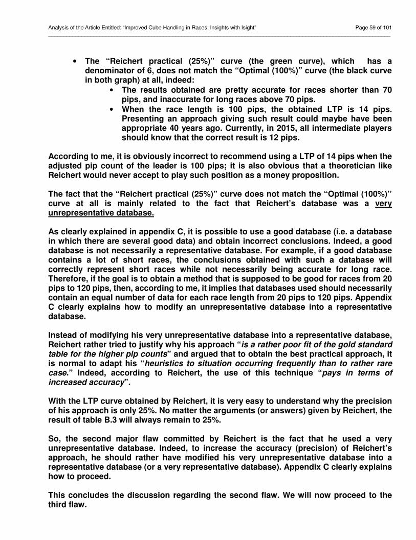
Analysis of the Article Entitled: “Improved Cube Handling in Races: Insights with Isight” Page 59 of 101 _________________________________________________________________________________________________________________
• The “Reichert practical (25%)” curve (the green curve), which has a denominator of 6, does not match the “Optimal (100%)” curve (the black curve in both graph) at all, indeed:
• The results obtained are pretty accurate for races shorter than 70 pips, and inaccurate for long races above 70 pips.
• When the race length is 100 pips, the obtained LTP is 14 pips. Presenting an approach giving such result could maybe have been appropriate 40 years ago. Currently, in 2015, all intermediate players should know that the correct result is 12 pips.
According to me, it is obviously incorrect to recommend using a LTP of 14 pips when the adjusted pip count of the leader is 100 pips; it is also obvious that a theoretician like Reichert would never accept to play such position as a money proposition. The fact that the “Reichert practical (25%)” curve does not match the “Optimal (100%)’’ curve at all is mainly related to the fact that Reichert’s database was a very unrepresentative database. As clearly explained in appendix C, it is possible to use a good database (i.e. a database in which there are several good data) and obtain incorrect conclusions. Indeed, a good database is not necessarily a representative database. For example, if a good database contains a lot of short races, the conclusions obtained with such a database will correctly represent short races while not necessarily being accurate for long race. Therefore, if the goal is to obtain a method that is supposed to be good for races from 20 pips to 120 pips, then, according to me, it implies that databases used should necessarily contain an equal number of data for each race length from 20 pips to 120 pips. Appendix C clearly explains how to modify an unrepresentative database into a representative database. Instead of modifying his very unrepresentative database into a representative database, Reichert rather tried to justify why his approach “is a rather poor fit of the gold standard table for the higher pip counts” and argued that to obtain the best practical approach, it is normal to adapt his “heuristics to situation occurring frequently than to rather rare case.” Indeed, according to Reichert, the use of this technique “pays in terms of increased accuracy”. With the LTP curve obtained by Reichert, it is very easy to understand why the precision of his approach is only 25%. No matter the arguments (or answers) given by Reichert, the result of table B.3 will always remain to 25%. So, the second major flaw committed by Reichert is the fact that he used a very unrepresentative database. Indeed, to increase the accuracy (precision) of Reichert’s approach, he should rather have modified his very unrepresentative database into a representative database (or a very representative database). Appendix C clearly explains how to proceed. This concludes the discussion regarding the second flaw. We will now proceed to the third flaw.

Analysis of the Article Entitled: “Improved Cube Handling in Races: Insights with Isight” Page 60 of 101 _________________________________________________________________________________________________________________
+ + + + + As already explained, before I exchanged email with Reichert, I thought that to develop his approach, the technique used contained “only” two major flaws. After the email exchange, I was rather convinced that a third major flaw was involved to develop his approach. The third flaw is that according to Reichert, to determine what is the best practical approach, the objective is to find the approach giving the “smallest total error regarding cube decisions” in relation to a “database containing about 50,000 real-life positions, with and without wastage”.; while the correct objective is to find the approach giving the best precision (i.e. the best percentage of good results) in relation to the best theoretical approach (i.e. the OPTIMAL APPROACH). The fact that Reichert used a different objective has as direct consequence on the way he would calculate and compare the financial results of his approach. That way to calculate and compare financial results is certainly different than mine. I can’t elaborate further on this topic because I do not know how Reichert would make these calculations, by taking into account each 303 possible results. However, I am convinced that Reichert will never be able to invalidate that the precision of his approach is 25%. I am also convinced that Reichert will never be able to demonstrate that the results presented in appendix D are wrong. To be able to develop any more on this third flaw, Reichert has to accept the two following challenges:
Challenge no:
Description
1 Reichert should present a clear table (similar to the Appendix D) giving his own expected conclusion, for each 303 values necessary to represent an approach.
2 Reichert should clearly mention if he would accept, yes or no, to play a money proposition for each of the 197 positions in which, according to Appendix D, Chabot’s approach should win.
This concludes the discussion regarding the third flaw. We will now give the summary of the big picture.
+ + + + +
Analysis of the Article Entitled: “Improved Cube Handling in Races: Insights with Isight” Page 61 of 101 _________________________________________________________________________________________________________________
It is possible to summarize the whole explanation presented so far as follow:
• With the optimal approach: o The database used was a very representative database; indeed, 50% of
races are shorter than 70 pips and 50% are above 70 pips, therefore, this approach is very accurate.
o The three obtained curves are curved; therefore, this approach is a theoretical approach. Each curve cannot be represented with a single slope (see graph 2.2 presented in section 2.1). Since each curve has an irregular slope, there are no specific denominators.
o The RW is pretty constant. o The DW is not constant. o This approach is considered as being the reference; therefore, the precision
of that approach is defined as 100%.
• With Chabot’s approach: o This approach is based on the optimal approach. The optimal approach is a
very accurate approach because the database used to obtain the optimal approach was a very representative database. Consequently, Chabot’s approach was also obtained by using the same very representative database. So, Chabot’s approach is a very reliable approach.
o The three obtained curves are straight lines; therefore, this is a practical approach. Each curve can be represented with a specific slope (see graph 6.2 presented in section 2.4).
� The denominator for the LTP curve is: 8, which means that the slope is 12.5%.
� The denominator for the RP curve is: 8, which means that the slope is 12.5%.
� The slope for the DP curve is 11%. o The RW is constant. o The DW is not constant because the slopes of the LTP and RP curves are
different. o The precision is 67%.
• With Reichert’s approach: o The database used was a very unrepresentative database; indeed, 90% of
races are shorter than 70 pips and 10% are above 70 pips. Therefore, this approach is unreliable and inaccurate.
o The three obtained curves are “straight” lines; therefore, this is a practical approach. Each curve can be represented with a specific slope (see graph B.2 presented in section 2.7).
� The denominator for the LTP curve is 6, which means that the slope is 16.7%.
� The denominator for the RP curve is 6, which means that the slope is 16.7%.
� The denominator for the DP curve is 6, which means that the slope is 16.7%.

Analysis of the Article Entitled: “Improved Cube Handling in Races: Insights with Isight” Page 62 of 101 _________________________________________________________________________________________________________________
o The RW is constant. o The DW is constant because the slope of the LTP and RP curve are the
same. o The precision is 25%.
+ + + + +
Given that Reichert mentioned that Trice criterion “gives extremely accurate cube decisions”; given that Trice’s approach almost perfectly matches the optimal approach; and given that Reichert’s curves do not match at all the optimal curve; it is very difficult to understand why Reichert could seriously pretend that his approach is more reliable that the optimal one. On one hand, Reichert admits that his LTP curve “is a rather poor fit of the gold standard table for the higher pip counts” and on the other hand, he pretends that his approach is the best approach proposed so far. According to me, this is a very obvious contradiction. Therefore, it is very difficult to give credibility to these specific results presented by Reichert.
In others words, according to me:
• If the optimal approach (and/or the “Gold standard Table”, and/or Trice’s approach, and/or Chabot’s approach) “gives extremely accurate cube decisions” and
• if Reichert’s approach does not match the optimal approach at all (and/or Chabot’s approach),
it necessarily implies that Reichert’s approach does not “give extremely accurate cube decisions” and that therefore Reichert’s approach could not be the best approach proposed so far. As already mentioned, I am really convinced that If Reichert had considered that the DW is not constant and if he had modified his very unrepresentative database to obtain a representative database; then, he would have certainly obtained an approach in which the denominator for the LTP curve is 8 (instead of 6) and he would certainly have obtained an approach much more reliable than the obtained approach. According to me, it is even possible that Reichert’s optimization work could have validated that Chabot’s approach is the best one. In section 2.11 entitled “Financial results: Reichert’s approach vs Chabot’s approach”, I challenged Reichert to prove that the content of Appendix D is wrong. According to me, Reichert can’t accept this challenge because he will never be able to prove that the content of the Appendix D is wrong.
+ + + + +
Analysis of the Article Entitled: “Improved Cube Handling in Races: Insights with Isight” Page 63 of 101 _________________________________________________________________________________________________________________
Chapter 3: Comments on Reichert’s adjustments As clearly mentioned in the introduction, this article will not analyze subjects other than Reichert’s approach. So, in this chapter, I will not analyze Reichert’s adjustments, only comment on them. On page 4 of his article, Reichert mentioned that “Pip counts need to be adjusted because straight (unadjusted) pip counts do a poor job when judging your racing chances.” On this specific point, I obviously agreed with Reichert. To calculate the adjusted pip count of both players, it is necessary to calculate the “straight” pip count and to add “pip count adjustments”. On page 12 of his article, Reichert presented Table 1 entitled “Parameters for adjusted pip counts” which contains 19 parameters. Each parameter has a lower limit and an upper limit. According to me, the upper limit for the stacks and for the gaps should have been higher. Using table 1 (in which I consider that some parameter might have a higher upper Reichert’s adjustments: limit), and using his database (which is a very unrepresentative database); Reichert has done an optimization work in order to obtain the best pip count adjustments. Here are Reichert’s adjustments:
• Add 1 pip for each additional checker on the board compared to the opponent. • Add 2 pips for each checker more than 2 on point 1.
• Add 1 pip for each checker more than 2 on point 2.
• Add 1 pip for each checker more than 3 on point 3.
• Add 1 pip for each empty space on points 4, 5, or 6 (only if the other player has a checker on his corresponding point).
• Add 1 pip for each additional crossover compared to the opponent. On page 36 of his article, Reichert presented Table 9 entitled “Combinations and error”. This table clearly demonstrates that all approaches benefit when they are combined with any pip count adjustments. That table also demonstrates that the best pip count adjustments obtained so far are Reichert’s. Consequently, it implies that:
• To use any approach, including the approaches conceived for low-wastage position like the optimal approach or the Chabot’s approach, it is necessary to use an adjusted pip count.
• The best pip count adjustments obtained so far are Reichert’s. Even if the best adjustments so far are Reichert’s; according to me, it may be possible to further improve the accuracy of Reichert’s adjustments because:
• The upper limit for some parameters might have possibly been higher.
• The database used was a very unrepresentative database.
Analysis of the Article Entitled: “Improved Cube Handling in Races: Insights with Isight” Page 64 of 101 _________________________________________________________________________________________________________________
Chapter 4: Comments on Reichert’s article As clearly mentioned in the introduction, I will comment about all topics developed in Reichert’s article. Reichert's approach was covered in Chapter 2; Reichert's adjustments were covered in Chapter 3. I also mentioned that I would not analyze subject other than Reichert’s approach. So, in this chapter, I will not analyze any topics and will simply make a few comments on the rest of his article. The main goal of Reichert’s article was probably to present his method that he called “the Isight method”. In others terms, the main goals of Reichert’s article were probably to present his approach and his adjustments. Reichert’s approach has been exhaustively analyzed in chapter 2. Reichert’s adjustments have been summarily commented in chapter 3. Excluding his approach and adjustments, Reichert’s article also presented many new ideas (or new concepts) regarding:
• Technique to calculate the adjusted pip count (see pages 11 to 15); • EPC (the Effective Pip Count, see pages 19 to 21).
• CPW (the Cubeless Probability of Winning, see pages 21 to 24).
• Transformation formula to convert any approach into an equivalent approach working with winning percentage (see pages 24 to 27).
It is certain that this article will improve the theory of cube handling in race for money games because Reichert presented many new ideas (or new concepts). The main goal of this article really is not to diminish the outstanding work done by Reichert; but, Reichert’s approach contains three major flaws and it was necessary to try to correct them. Even if Reichert’s approach is an unreliable approach because it contains three major flaws, the other subjects developed in his article are nevertheless very interesting and could be very reliable and very accurate.
+ + + + +
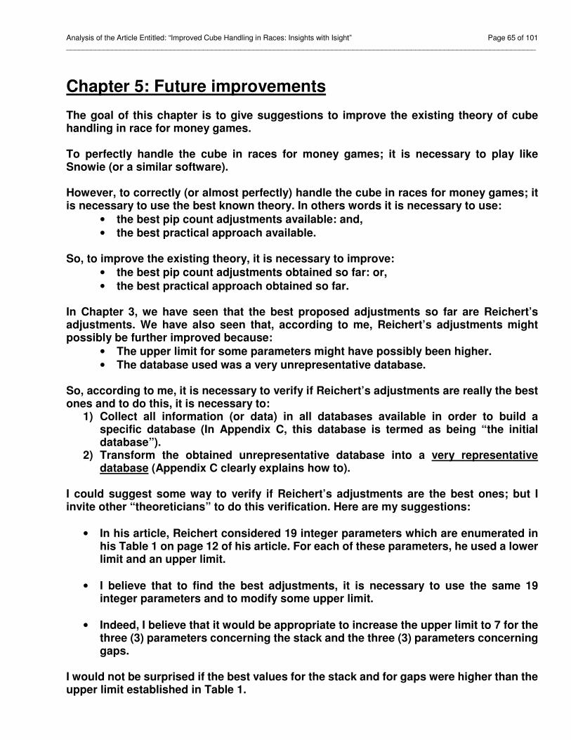
Analysis of the Article Entitled: “Improved Cube Handling in Races: Insights with Isight” Page 65 of 101 _________________________________________________________________________________________________________________
Chapter 5: Future improvements The goal of this chapter is to give suggestions to improve the existing theory of cube handling in race for money games. To perfectly handle the cube in races for money games; it is necessary to play like Snowie (or a similar software). However, to correctly (or almost perfectly) handle the cube in races for money games; it is necessary to use the best known theory. In others words it is necessary to use:
• the best pip count adjustments available: and, • the best practical approach available.
So, to improve the existing theory, it is necessary to improve:
• the best pip count adjustments obtained so far: or,
• the best practical approach obtained so far. In Chapter 3, we have seen that the best proposed adjustments so far are Reichert’s adjustments. We have also seen that, according to me, Reichert’s adjustments might possibly be further improved because:
• The upper limit for some parameters might have possibly been higher. • The database used was a very unrepresentative database.
So, according to me, it is necessary to verify if Reichert’s adjustments are really the best ones and to do this, it is necessary to:
1) Collect all information (or data) in all databases available in order to build a specific database (In Appendix C, this database is termed as being “the initial database”).
2) Transform the obtained unrepresentative database into a very representative database (Appendix C clearly explains how to).
I could suggest some way to verify if Reichert’s adjustments are the best ones; but I invite other “theoreticians” to do this verification. Here are my suggestions:
• In his article, Reichert considered 19 integer parameters which are enumerated in his Table 1 on page 12 of his article. For each of these parameters, he used a lower limit and an upper limit.
• I believe that to find the best adjustments, it is necessary to use the same 19 integer parameters and to modify some upper limit.
• Indeed, I believe that it would be appropriate to increase the upper limit to 7 for the three (3) parameters concerning the stack and the three (3) parameters concerning gaps.
I would not be surprised if the best values for the stack and for gaps were higher than the upper limit established in Table 1.
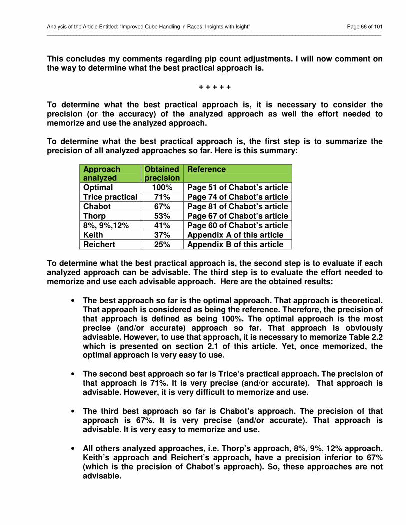
Analysis of the Article Entitled: “Improved Cube Handling in Races: Insights with Isight” Page 66 of 101 _________________________________________________________________________________________________________________
This concludes my comments regarding pip count adjustments. I will now comment on the way to determine what the best practical approach is.
+ + + + + To determine what the best practical approach is, it is necessary to consider the precision (or the accuracy) of the analyzed approach as well the effort needed to memorize and use the analyzed approach. To determine what the best practical approach is, the first step is to summarize the precision of all analyzed approaches so far. Here is this summary:
Approach analyzed
Obtained precision
Reference
Optimal 100% Page 51 of Chabot’s article Trice practical 71% Page 74 of Chabot’s article Chabot 67% Page 81 of Chabot’s article Thorp 53% Page 67 of Chabot’s article 8%, 9%,12% 41% Page 60 of Chabot’s article Keith 37% Appendix A of this article Reichert 25% Appendix B of this article
To determine what the best practical approach is, the second step is to evaluate if each analyzed approach can be advisable. The third step is to evaluate the effort needed to memorize and use each advisable approach. Here are the obtained results:
• The best approach so far is the optimal approach. That approach is theoretical. That approach is considered as being the reference. Therefore, the precision of that approach is defined as being 100%. The optimal approach is the most precise (and/or accurate) approach so far. That approach is obviously advisable. However, to use that approach, it is necessary to memorize Table 2.2 which is presented on section 2.1 of this article. Yet, once memorized, the optimal approach is very easy to use.
• The second best approach so far is Trice’s practical approach. The precision of that approach is 71%. It is very precise (and/or accurate). That approach is advisable. However, it is very difficult to memorize and use.
• The third best approach so far is Chabot’s approach. The precision of that approach is 67%. It is very precise (and/or accurate). That approach is advisable. It is very easy to memorize and use.
• All others analyzed approaches, i.e. Thorp’s approach, 8%, 9%, 12% approach, Keith’s approach and Reichert’s approach, have a precision inferior to 67% (which is the precision of Chabot’s approach). So, these approaches are not advisable.
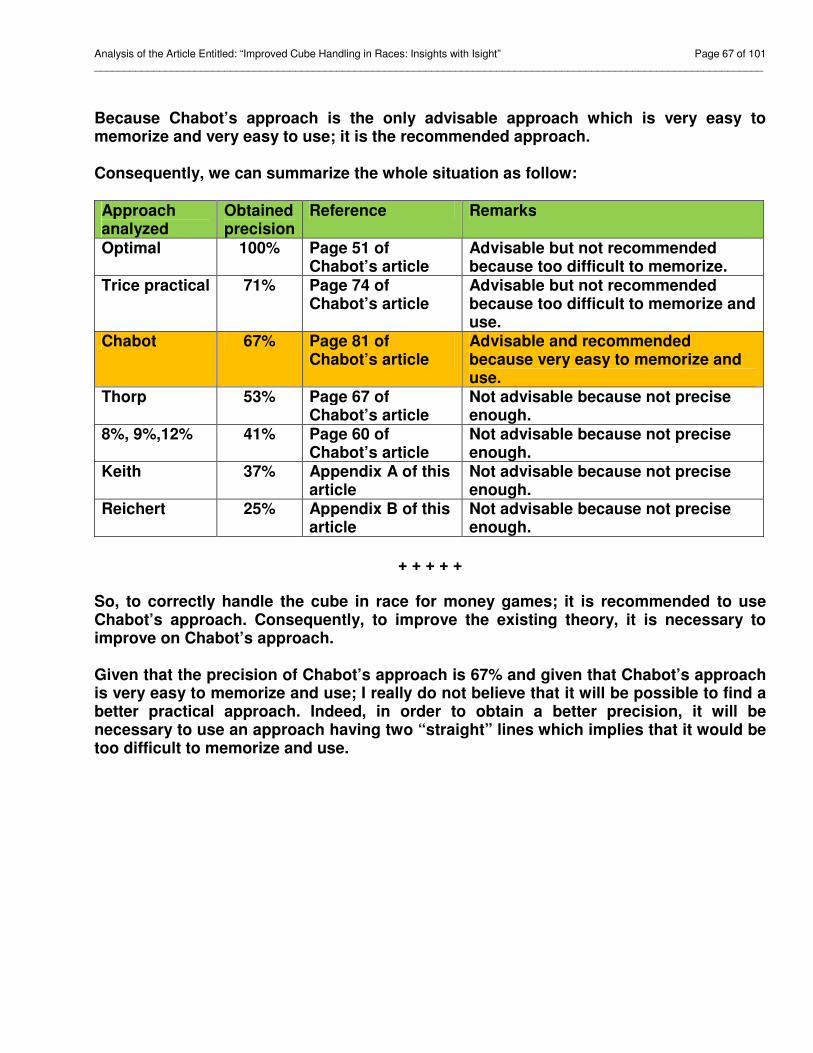
Analysis of the Article Entitled: “Improved Cube Handling in Races: Insights with Isight” Page 67 of 101 _________________________________________________________________________________________________________________
Because Chabot’s approach is the only advisable approach which is very easy to memorize and very easy to use; it is the recommended approach. Consequently, we can summarize the whole situation as follow: Approach analyzed
Obtained precision
Reference Remarks
Optimal 100% Page 51 of Chabot’s article
Advisable but not recommended because too difficult to memorize.
Trice practical 71% Page 74 of Chabot’s article
Advisable but not recommended because too difficult to memorize and use.
Chabot 67% Page 81 of Chabot’s article
Advisable and recommended because very easy to memorize and use.
Thorp 53% Page 67 of Chabot’s article
Not advisable because not precise enough.
8%, 9%,12% 41% Page 60 of Chabot’s article
Not advisable because not precise enough.
Keith 37% Appendix A of this article
Not advisable because not precise enough.
Reichert 25% Appendix B of this article
Not advisable because not precise enough.
+ + + + +
So, to correctly handle the cube in race for money games; it is recommended to use Chabot’s approach. Consequently, to improve the existing theory, it is necessary to improve on Chabot’s approach. Given that the precision of Chabot’s approach is 67% and given that Chabot’s approach is very easy to memorize and use; I really do not believe that it will be possible to find a better practical approach. Indeed, in order to obtain a better precision, it will be necessary to use an approach having two “straight” lines which implies that it would be too difficult to memorize and use.
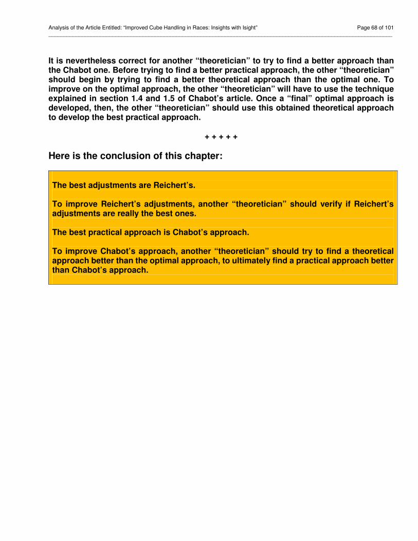
Analysis of the Article Entitled: “Improved Cube Handling in Races: Insights with Isight” Page 68 of 101 _________________________________________________________________________________________________________________
It is nevertheless correct for another “theoretician” to try to find a better approach than the Chabot one. Before trying to find a better practical approach, the other “theoretician” should begin by trying to find a better theoretical approach than the optimal one. To improve on the optimal approach, the other “theoretician” will have to use the technique explained in section 1.4 and 1.5 of Chabot’s article. Once a “final” optimal approach is developed, then, the other “theoretician” should use this obtained theoretical approach to develop the best practical approach.
+ + + + +
Here is the conclusion of this chapter: The best adjustments are Reichert’s. To improve Reichert’s adjustments, another “theoretician” should verify if Reichert’s adjustments are really the best ones. The best practical approach is Chabot’s approach. To improve Chabot’s approach, another “theoretician” should try to find a theoretical approach better than the optimal approach, to ultimately find a practical approach better than Chabot’s approach.

Analysis of the Article Entitled: “Improved Cube Handling in Races: Insights with Isight” Page 69 of 101 _________________________________________________________________________________________________________________
Conclusion
The main goal of this article was to clearly explain: • what are the three flaws involved in the development of Reichert’s approach; and, • why Reichert’s approach is the worst approach proposed so far.
Here are the three flaws involved in the development of Reichert’s approach:
1) Reichert used a wrong hypothesis. Indeed, according to the optimal approach, the DW (Doubling Window) is not constant. Reichert has not verified whether the DW is constant or not; and he incorrectly assumed that the DW is constant.
2) Reichert used a wrong database. Indeed, Reichert should have used a representative database or a very representative database. He incorrectly used a very unrepresentative database.
3) Reichert used a wrong objective. Indeed, Reichert should have chosen the objective to optimize the precision (i.e. the best percentage of good results) using the optimal approach as a reference. He has wrongly chosen the objective by choosing the smallest total error regarding cube decisions in relation to a very unrepresentative database.
Reichert’s approach is the worst approach proposed so far because the precision is ONLY 25%; which is the worst precision obtained so far. Regarding the optimal approach, we have seen that:
• That approach is the best theoretical approach proposed so far.
• That approach was elaborated with great detail to allow any skeptical reader to verify its accuracy.
• It is very easy to verify the accuracy of this approach. • Before publishing his article, Reichert did not verify the accuracy of the optimal
approach.
• Reichert refused my challenge to verify the accuracy of the optimal approach. The graph entitled “The Optimal-Chabot-Trice curves” clearly illustrates that there is very little difference between the four following curves:
1) LTP theoretical curve of the optimal approach. 2) LTP theoretical curve as presented by Trice which, according to Reichert,
has been termed “Gold standard Table”. 3) LTP practical curve of Trice's approach which, according to Reichert, gives
“extremely accurate results”. 4) LTP practical curve of Chabot’s approach.
Cconsequently, the four above curves give very accurate results from 20 pips to 120 pips. The graph entitled “The Optimal-Chabot-Reichert curves” clearly illustrates that Reichert’s approach gives pretty accurate result for races shorter than 70 pips and very inaccurate results for races above 70 pips. Consequently, Reichert’s approach does not give accurate results for races from 20 pips to 120 pips.
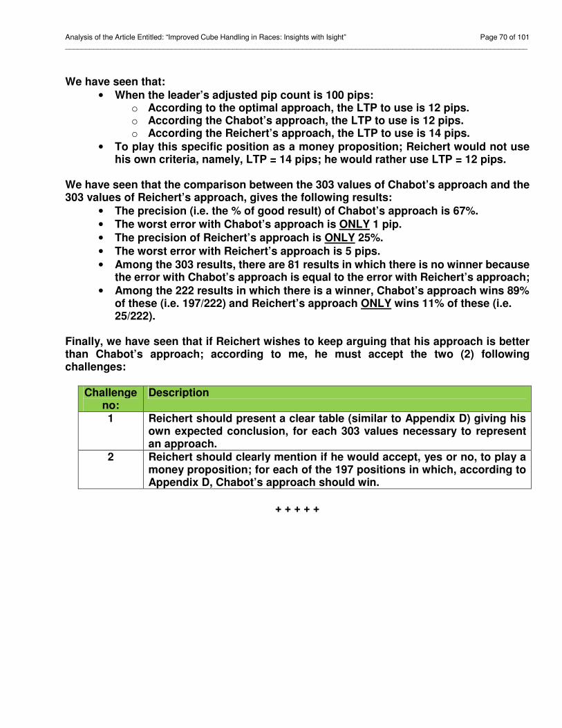
Analysis of the Article Entitled: “Improved Cube Handling in Races: Insights with Isight” Page 70 of 101 _________________________________________________________________________________________________________________
We have seen that:
• When the leader’s adjusted pip count is 100 pips: o According to the optimal approach, the LTP to use is 12 pips. o According the Chabot’s approach, the LTP to use is 12 pips. o According the Reichert’s approach, the LTP to use is 14 pips.
• To play this specific position as a money proposition; Reichert would not use his own criteria, namely, LTP = 14 pips; he would rather use LTP = 12 pips.
We have seen that the comparison between the 303 values of Chabot’s approach and the 303 values of Reichert’s approach, gives the following results:
• The precision (i.e. the % of good result) of Chabot’s approach is 67%. • The worst error with Chabot’s approach is ONLY 1 pip.
• The precision of Reichert’s approach is ONLY 25%.
• The worst error with Reichert’s approach is 5 pips. • Among the 303 results, there are 81 results in which there is no winner because
the error with Chabot’s approach is equal to the error with Reichert’s approach; • Among the 222 results in which there is a winner, Chabot’s approach wins 89%
of these (i.e. 197/222) and Reichert’s approach ONLY wins 11% of these (i.e. 25/222).
Finally, we have seen that if Reichert wishes to keep arguing that his approach is better than Chabot’s approach; according to me, he must accept the two (2) following challenges:
Challenge no:
Description
1 Reichert should present a clear table (similar to Appendix D) giving his own expected conclusion, for each 303 values necessary to represent an approach.
2 Reichert should clearly mention if he would accept, yes or no, to play a money proposition; for each of the 197 positions in which, according to Appendix D, Chabot’s approach should win.
+ + + + +
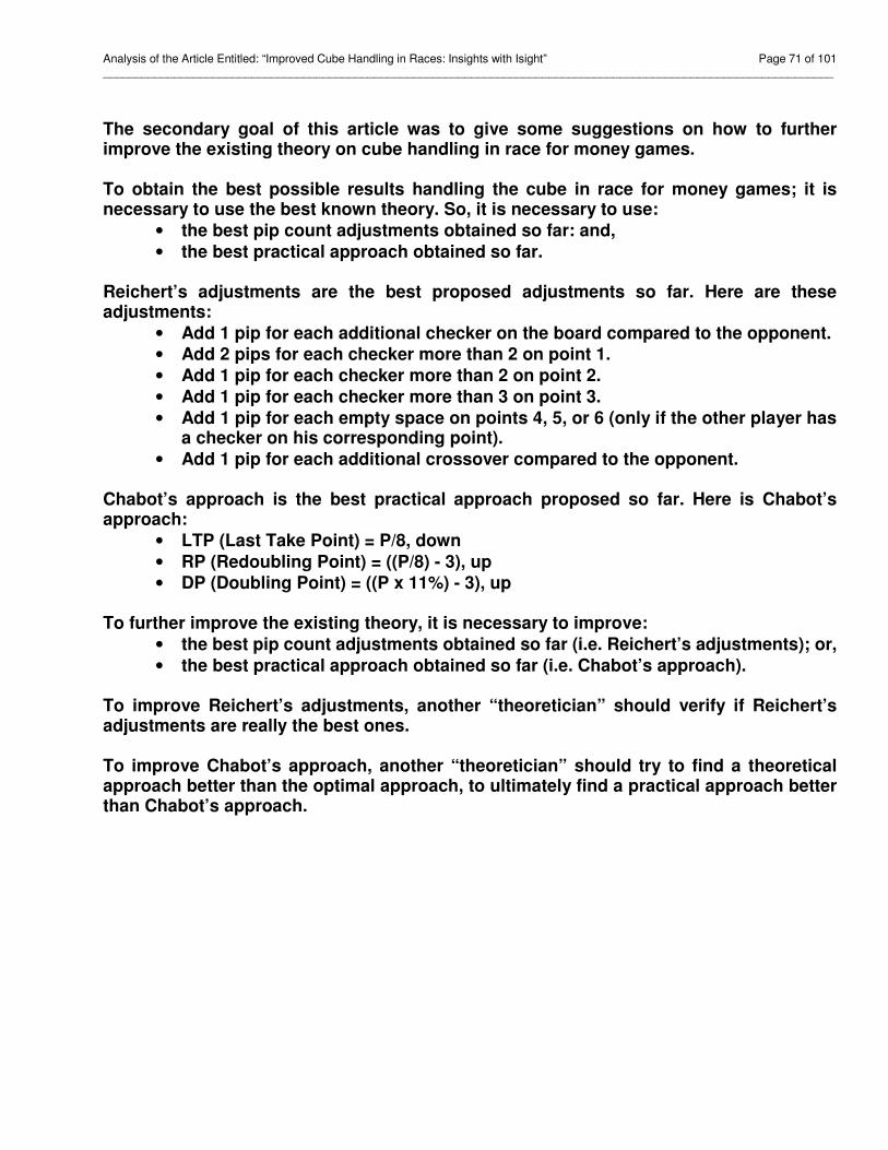
Analysis of the Article Entitled: “Improved Cube Handling in Races: Insights with Isight” Page 71 of 101 _________________________________________________________________________________________________________________
The secondary goal of this article was to give some suggestions on how to further improve the existing theory on cube handling in race for money games. To obtain the best possible results handling the cube in race for money games; it is necessary to use the best known theory. So, it is necessary to use:
• the best pip count adjustments obtained so far: and,
• the best practical approach obtained so far. Reichert’s adjustments are the best proposed adjustments so far. Here are these adjustments:
• Add 1 pip for each additional checker on the board compared to the opponent. • Add 2 pips for each checker more than 2 on point 1.
• Add 1 pip for each checker more than 2 on point 2.
• Add 1 pip for each checker more than 3 on point 3. • Add 1 pip for each empty space on points 4, 5, or 6 (only if the other player has
a checker on his corresponding point). • Add 1 pip for each additional crossover compared to the opponent.
Chabot’s approach is the best practical approach proposed so far. Here is Chabot’s approach:
• LTP (Last Take Point) = P/8, down • RP (Redoubling Point) = ((P/8) - 3), up • DP (Doubling Point) = ((P x 11%) - 3), up
To further improve the existing theory, it is necessary to improve:
• the best pip count adjustments obtained so far (i.e. Reichert’s adjustments); or,
• the best practical approach obtained so far (i.e. Chabot’s approach). To improve Reichert’s adjustments, another “theoretician” should verify if Reichert’s adjustments are really the best ones.
To improve Chabot’s approach, another “theoretician” should try to find a theoretical approach better than the optimal approach, to ultimately find a practical approach better than Chabot’s approach.
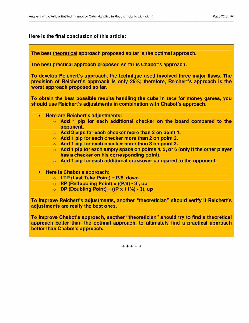
Analysis of the Article Entitled: “Improved Cube Handling in Races: Insights with Isight” Page 72 of 101 _________________________________________________________________________________________________________________
Here is the final conclusion of this article: The best theoretical approach proposed so far is the optimal approach. The best practical approach proposed so far is Chabot’s approach. To develop Reichert’s approach, the technique used involved three major flaws. The precision of Reichert’s approach is only 25%; therefore, Reichert’s approach is the worst approach proposed so far. To obtain the best possible results handling the cube in race for money games, you should use Reichert’s adjustments in combination with Chabot’s approach.
• Here are Reichert’s adjustments:
o Add 1 pip for each additional checker on the board compared to the opponent.
o Add 2 pips for each checker more than 2 on point 1. o Add 1 pip for each checker more than 2 on point 2. o Add 1 pip for each checker more than 3 on point 3. o Add 1 pip for each empty space on points 4, 5, or 6 (only if the other player
has a checker on his corresponding point). o Add 1 pip for each additional crossover compared to the opponent.
• Here is Chabot’s approach:
o LTP (Last Take Point) = P/8, down o RP (Redoubling Point) = ((P/8) - 3), up o DP (Doubling Point) = ((P x 11%) - 3), up
To improve Reichert’s adjustments, another “theoretician” should verify if Reichert’s adjustments are really the best ones.
To improve Chabot’s approach, another “theoretician” should try to find a theoretical approach better than the optimal approach, to ultimately find a practical approach better than Chabot’s approach.
+ + + + +

Analysis of the Article Entitled: “Improved Cube Handling in Races: Insights with Isight” Page 73 of 101 _________________________________________________________________________________________________________________
Appendix A: Keith’s approach Even if Keith’s approach was published in June 2004, this approach could be considered as relatively new. Keith’s approach can be found on the Backgammon Galore! Website at: http://www.bkgm.com/articles/CubeHandlingInRaces/ The decision criteria of this approach are:
DP = ((P/7) - 4), up RP = ((P/7) - 3), up LTP = ((P/7) - 2), down
Table A.1 presents the obtained values. Graph A.1 illustrates the obtained LTP values. Marginal decision points are highlighted. Graph A.2 illustrates the obtained RP values. Marginal decision points are highlighted. Graph A.3 illustrates the obtained DP values. Marginal decision points are highlighted. Graph A.4 illustrates the obtained LTP, RP and DP values. Marginal decision points are highlighted. Table A.2 presents the summary of the obtained values. Using this approach, when "P" (the leader’s pip count) is 100 pips, then:
• The leader must double if the trailer’s pip count is equal or superior to 110 pips. • The leader must redouble if the trailer’s pip count is equal or superior to 111 pips. • The trailer must take if his pip count is equal or inferior to 112 pips.
Using this approach, when "P" (the leader’s pip count) is 50 pips, then:
• The leader must double if the trailer’s pip count is equal or superior to 53 pips.
• The leader must redouble if the trailer’s pip count is equal or superior to 54 pips. • The trailer must take if his pip count is equal or inferior to 55 pips.
Table A.3 presents the calculations of the precision. The results obtained are:
Good results: ............................................... 37.0% Results with a 1-pip difference: ................. 41.9% Results with a 2-pip difference: ................. 17.8% Results with a 3-pip difference: ................... 3.3%
Graph A.5 compares the marginal decision points curves of this approach to the optimal approach.
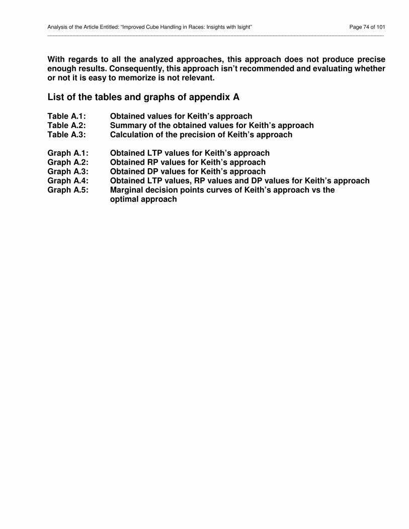
Analysis of the Article Entitled: “Improved Cube Handling in Races: Insights with Isight” Page 74 of 101 _________________________________________________________________________________________________________________
With regards to all the analyzed approaches, this approach does not produce precise enough results. Consequently, this approach isn’t recommended and evaluating whether or not it is easy to memorize is not relevant.
List of the tables and graphs of appendix A Table A.1: Obtained values for Keith’s approach Table A.2: Summary of the obtained values for Keith’s approach Table A.3: Calculation of the precision of Keith’s approach Graph A.1: Obtained LTP values for Keith’s approach Graph A.2: Obtained RP values for Keith’s approach Graph A.3: Obtained DP values for Keith’s approach Graph A.4: Obtained LTP values, RP values and DP values for Keith’s approach Graph A.5: Marginal decision points curves of Keith’s approach vs the
optimal approach

Analysis of the Article Entitled: “Improved Cube Handling in Races: Insights with Isight” Page 75 of 101 _________________________________________________________________________________________________________________
Table A.1: Obtained values for Keith's approach
P DP RP LTP P DP RP LTP
20 -2 -1 0 71 6 7 8
21 -1 0 1 72 6 7 8
22 -1 0 1 73 6 7 8
23 -1 0 1 74 6 7 8
24 -1 0 1 75 6 7 8
25 -1 0 1 76 6 7 8
26 -1 0 1 77 7 8 9
27 -1 0 1 78 7 8 9
28 0 1 2 79 7 8 9
29 0 1 2 80 7 8 9
30 0 1 2 81 7 8 9
31 0 1 2 82 7 8 9
32 0 1 2 83 7 8 9
33 0 1 2 84 8 9 10
34 0 1 2 85 8 9 10
35 1 2 3 86 8 9 10
36 1 2 3 87 8 9 10
37 1 2 3 88 8 9 10
38 1 2 3 89 8 9 10
39 1 2 3 90 8 9 10
40 1 2 3 91 9 10 11
41 1 2 3 92 9 10 11
42 2 3 4 93 9 10 11
43 2 3 4 94 9 10 11
44 2 3 4 95 9 10 11
45 2 3 4 96 9 10 11
46 2 3 4 97 9 10 11
47 2 3 4 98 10 11 12
48 2 3 4 99 10 11 12
49 3 4 5 100 10 11 12
50 3 4 5 101 10 11 12
51 3 4 5 102 10 11 12
52 3 4 5 103 10 11 12
53 3 4 5 104 10 11 12
54 3 4 5 105 11 12 13
55 3 4 5 106 11 12 13
56 4 5 6 107 11 12 13
57 4 5 6 108 11 12 13
58 4 5 6 109 11 12 13
59 4 5 6 110 11 12 13
60 4 5 6 111 11 12 13
61 4 5 6 112 12 13 14
62 4 5 6 113 12 13 14
63 5 6 7 114 12 13 14
64 5 6 7 115 12 13 14
65 5 6 7 116 12 13 14
66 5 6 7 117 12 13 14
67 5 6 7 118 12 13 14
68 5 6 7 119 13 14 15
69 5 6 7 120 13 14 15
70 6 7 8

Analysis of the Article Entitled: “Improved Cube Handling in Races: Insights with Isight” Page 76 of 101 _________________________________________________________________________________________________________________
Table A.2: Summary of the obtained values for Keith's approach
Leader's Leader Leader's Leader Leader's Trailer
adjusted should adjusted should adjusted should
pipcount double pipcount redouble pipcount take
if equal if equal if equalor up: or up: or down:
20 ─ 21 -2 20 ─ 21 -1 20 0
22 ─ 28 -1 22 ─ 28 0 21 ─ 27 1
29 ─ 35 0 29 ─ 35 1 28 ─ 34 2
36 ─ 42 1 36 ─ 42 2 35 ─ 41 3
43 ─ 49 2 43 ─ 49 3 42 ─ 48 4
50 ─ 56 3 50 ─ 56 4 49 ─ 55 5
57 ─ 63 4 57 ─ 63 5 56 ─ 62 6
64 ─ 70 5 64 ─ 70 6 63 ─ 69 7
71 ─ 77 6 71 ─ 77 7 70 ─ 76 8
78 ─ 84 7 78 ─ 84 8 77 ─ 83 9
85 ─ 91 8 85 ─ 91 9 84 ─ 90 10
92 ─ 98 9 92 ─ 98 10 91 ─ 97 11
99 ─ 105 10 99 ─ 105 11 98 ─ 104 12
106 ─ 112 11 106 ─ 112 12 105 ─ 111 13
113 ─ 119 12 113 ─ 119 13 112 ─ 118 14
120 13 120 14 119 ─ 120 15
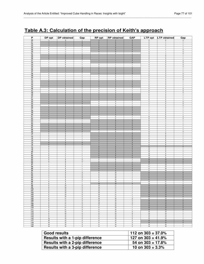
Analysis of the Article Entitled: “Improved Cube Handling in Races: Insights with Isight” Page 77 of 101 _________________________________________________________________________________________________________________
Table A.3: Calculation of the precision of Keith's approach
P DP opt DP obtained Gap RP opt RP obtained GAP LTP opt LTP obtained Gap20 -1 -2 1 -1 -1 0 2 0 2
21 -1 -1 0 0 0 0 2 1 1
22 -1 -1 0 0 0 0 2 1 1
23 -1 -1 0 0 0 0 2 1 1
24 0 -1 1 0 0 0 2 1 1
25 0 -1 1 0 0 0 3 1 2
26 0 -1 1 0 0 0 3 1 2
27 0 -1 1 1 0 1 3 1 2
28 0 0 0 1 1 0 3 2 1
29 0 0 0 1 1 0 3 2 1
30 0 0 0 1 1 0 3 2 1
31 1 0 1 1 1 0 4 2 2
32 1 0 1 1 1 0 4 2 2
33 1 0 1 2 1 1 4 2 2
34 1 0 1 2 1 1 4 2 2
35 1 1 0 2 2 0 4 3 1
36 1 1 0 2 2 0 4 3 1
37 1 1 0 2 2 0 4 3 1
38 2 1 1 2 2 0 5 3 2
39 2 1 1 3 2 1 5 3 2
40 2 1 1 3 2 1 5 3 2
41 2 1 1 3 2 1 5 3 2
42 2 2 0 3 3 0 5 4 1
43 2 2 0 3 3 0 5 4 1
44 2 2 0 3 3 0 5 4 1
45 2 2 0 3 3 0 5 4 1
46 3 2 1 4 3 1 6 4 2
47 3 2 1 4 3 1 6 4 2
48 3 2 1 4 3 1 6 4 2
49 3 3 0 4 4 0 6 5 1
50 3 3 0 4 4 0 6 5 1
51 3 3 0 4 4 0 6 5 1
52 3 3 0 4 4 0 6 5 1
53 3 3 0 5 4 1 7 5 2
54 3 3 0 5 4 1 7 5 2
55 4 3 1 5 4 1 7 5 2
56 4 4 0 5 5 0 7 6 1
57 4 4 0 5 5 0 7 6 1
58 4 4 0 5 5 0 7 6 1
59 4 4 0 5 5 0 7 6 1
60 4 4 0 5 5 0 7 6 1
61 4 4 0 6 5 1 8 6 2
62 4 4 0 6 5 1 8 6 2
63 4 5 1 6 6 0 8 7 1
64 4 5 1 6 6 0 8 7 1
65 5 5 0 6 6 0 8 7 1
66 5 5 0 6 6 0 8 7 1
67 5 5 0 6 6 0 8 7 1
68 5 5 0 6 6 0 8 7 1
69 5 5 0 7 6 1 9 7 2
70 5 6 1 7 7 0 9 8 1
71 5 6 1 7 7 0 9 8 1
72 5 6 1 7 7 0 9 8 1
73 5 6 1 7 7 0 9 8 1
74 5 6 1 7 7 0 9 8 1
75 6 6 0 7 7 0 9 8 1
76 6 6 0 7 7 0 9 8 1
77 6 7 1 8 8 0 9 9 0
78 6 7 1 8 8 0 10 9 1
79 6 7 1 8 8 0 10 9 1
80 6 7 1 8 8 0 10 9 1
81 6 7 1 8 8 0 10 9 1
82 6 7 1 8 8 0 10 9 1
83 6 7 1 8 8 0 10 9 1
84 6 8 2 8 9 1 10 10 0
85 6 8 2 8 9 1 10 10 0
86 7 8 1 9 9 0 10 10 0
87 7 8 1 9 9 0 11 10 1
88 7 8 1 9 9 0 11 10 1
89 7 8 1 9 9 0 11 10 1
90 7 8 1 9 9 0 11 10 1
91 7 9 2 9 10 1 11 11 0
92 7 9 2 9 10 1 11 11 0
93 7 9 2 9 10 1 11 11 0
94 7 9 2 9 10 1 11 11 0
95 7 9 2 9 10 1 11 11 0
96 8 9 1 9 10 1 12 11 1
97 8 9 1 10 10 0 12 11 1
98 8 10 2 10 11 1 12 12 0
99 8 10 2 10 11 1 12 12 0
100 8 10 2 10 11 1 12 12 0
101 8 10 2 10 11 1 12 12 0
102 8 10 2 10 11 1 12 12 0
103 8 10 2 10 11 1 12 12 0
104 8 10 2 10 11 1 12 12 0
105 8 11 3 10 12 2 12 13 1
106 8 11 3 10 12 2 13 13 0
107 9 11 2 10 12 2 13 13 0
108 9 11 2 10 12 2 13 13 0
109 9 11 2 11 12 1 13 13 0
110 9 11 2 11 12 1 13 13 0
111 9 11 2 11 12 1 13 13 0
112 9 12 3 11 13 2 13 14 1
113 9 12 3 11 13 2 13 14 1
114 9 12 3 11 13 2 13 14 1
115 9 12 3 11 13 2 13 14 1
116 10 12 2 11 13 2 13 14 1
117 10 12 2 11 13 2 14 14 0
118 10 12 2 11 13 2 14 14 0
119 10 13 3 11 14 3 14 15 1
120 10 13 3 11 14 3 14 15 1
Good results 112 on 303 = 37.0% Results with a 1-pip difference 127 on 303 = 41.9% Results with a 2-pip difference 54 on 303 = 17.8% Results with a 3-pip difference 10 on 303 = 3.3%
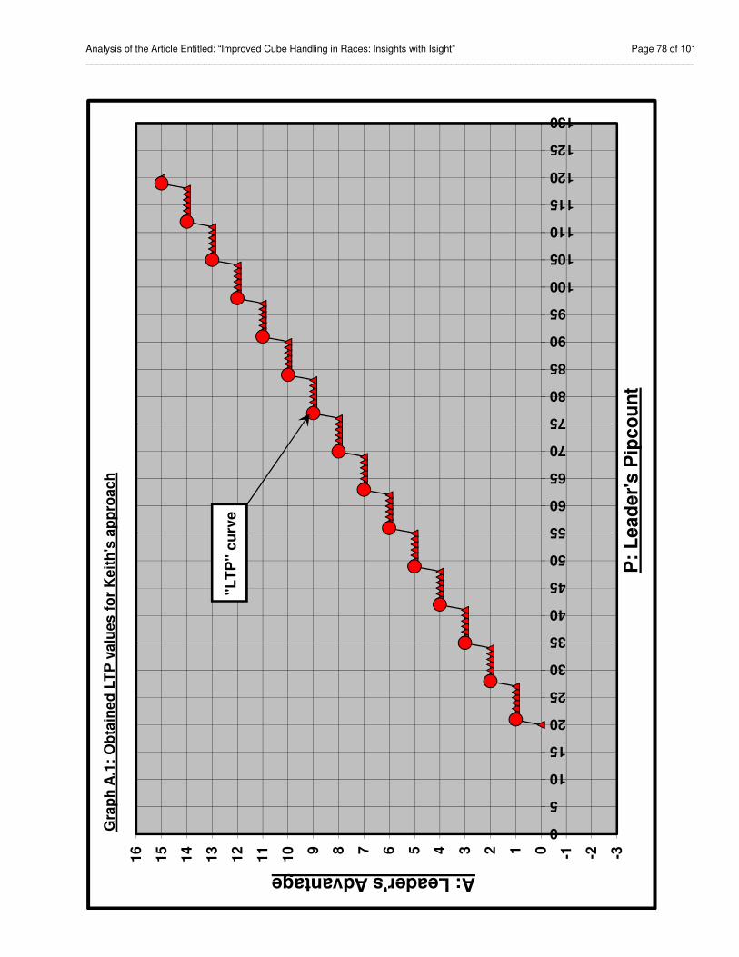
Analysis of the Article Entitled: “Improved Cube Handling in Races: Insights with Isight” Page 78 of 101 _________________________________________________________________________________________________________________
-3-2-10123456789
10
11
12
13
14
15
16
0
5
10
15
20
25
30
35
40
45
50
55
60
65
70
75
80
85
90
95
100
105
110
115
120
125
130
A: Leader's Advantage
P:
Le
ad
er'
s P
ipc
ou
nt
Gra
ph
A.1
: O
bta
ine
d L
TP
va
lue
s f
or
Ke
ith
's a
pp
roa
ch
"LT
P"
cu
rve
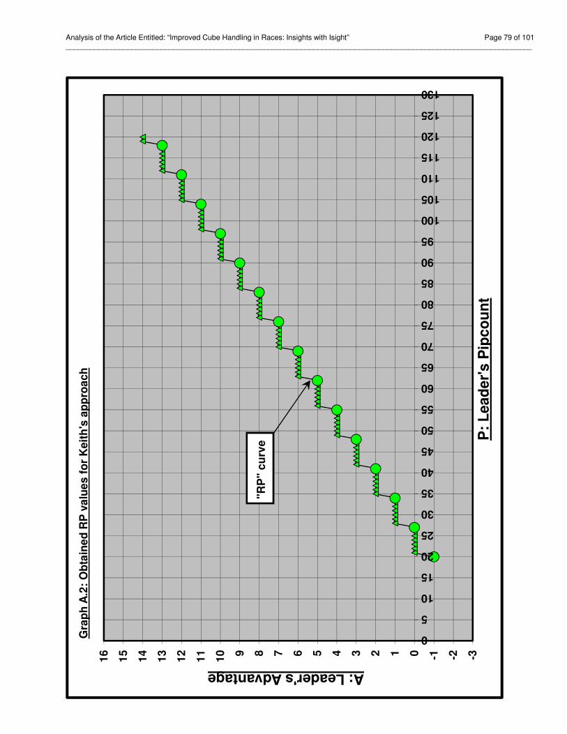
Analysis of the Article Entitled: “Improved Cube Handling in Races: Insights with Isight” Page 79 of 101 _________________________________________________________________________________________________________________
-3-2-10123456789
10
11
12
13
14
15
16
0
5
10
15
20
25
30
35
40
45
50
55
60
65
70
75
80
85
90
95
100
105
110
115
120
125
130
A: Leader's Advantage
P:
Le
ad
er'
s P
ipc
ou
nt
Gra
ph
A.2
: O
bta
ine
d R
P v
alu
es
fo
r K
eit
h's
ap
pro
ac
h
"RP
" c
urv
e
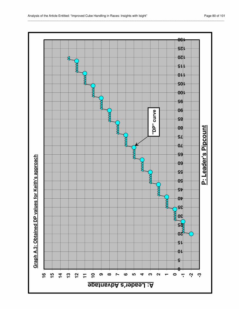
Analysis of the Article Entitled: “Improved Cube Handling in Races: Insights with Isight” Page 80 of 101 _________________________________________________________________________________________________________________
-3-2-10123456789
10
11
12
13
14
15
16
0
5
10
15
20
25
30
35
40
45
50
55
60
65
70
75
80
85
90
95
100
105
110
115
120
125
130
A: Leader's Advantage
P:
Le
ad
er'
s P
ipc
ou
nt
Gra
ph
A.3
: O
bta
ine
d D
P v
alu
es
fo
r K
eit
h's
ap
pro
ac
h
"DP
" c
urv
e
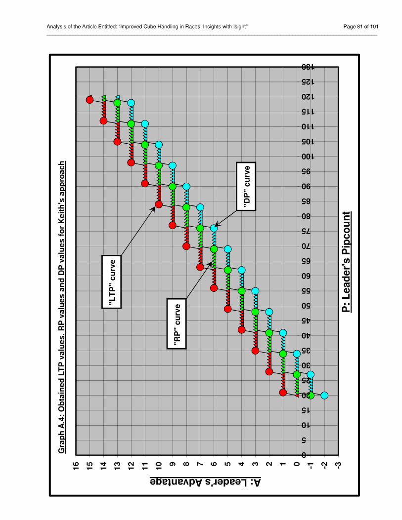
Analysis of the Article Entitled: “Improved Cube Handling in Races: Insights with Isight” Page 81 of 101 _________________________________________________________________________________________________________________
-3-2-10123456789
10
11
12
13
14
15
16
0
5
10
15
20
25
30
35
40
45
50
55
60
65
70
75
80
85
90
95
100
105
110
115
120
125
130
A: Leader's Advantage
P:
Lead
er'
s P
ipco
un
t
Gra
ph
A.4
: O
bta
ined
LT
P v
alu
es,
RP
valu
es a
nd
DP
valu
es f
or
Keit
h's
ap
pro
ach
"LT
P"
cu
rve
"RP
" c
urv
e
"DP
" c
urv
e

Analysis of the Article Entitled: “Improved Cube Handling in Races: Insights with Isight” Page 82 of 101 _________________________________________________________________________________________________________________
-3-2-101234567891011121314151617
0
5
10
15
20
25
30
35
40
45
50
55
60
65
70
75
80
85
90
95
100
105
110
115
120
125
130
A: Leader's Advantage
P:
Lea
der
's P
ipco
un
t
Gra
ph
A.5
: M
arg
inal
dec
isio
n p
oin
ts c
urv
es o
f K
eith
's a
pp
roac
h V
s th
e o
pti
mal
ap
pro
ach
DP
RP
LT
P
Co
lou
r: K
eit
h
Bla
ck
: O
pti
ma
l P
rec
isio
n:
37.0
%
Pre
cis
ion
: 4
1%
Analysis of the Article Entitled: “Improved Cube Handling in Races: Insights with Isight” Page 83 of 101 _________________________________________________________________________________________________________________
Appendix B: Reichert’s approach Reichert’s approach is a new approach. You can find it in Axel Reichert’s article at: http://www.bkgm.com/articles/Reichert/insights-with-isight.pdf To present Reichert's approach, he proposed two different techniques. The two proposed techniques that have been presented give exactly the same results. The first technique is called “the general technique” and the second technique is called “the specific technique”. The general technique can be used for match game and for money games while the specific technique can only be used for money games. Here is Reichert’s approach presented with mathematical formula that corresponds to the general technique:
��� = �� −�
+ �∆�
Here is the meaning of symbols used:
Symbol
used Meaning
��� Cubeless Probability of Winning
� Your adjusted pip count
∆� Your lead (could be negative)
• If ��� < 68: No double, take.
• If 68 ≤ ��� ≤ 70: Double, take.
• If 70 ≤ ��� ≤ 76: Redouble, take.
• If ��� > 76: Redouble, pass.
Here is Reichert’s approach presented with the mathematical formulas that correspond to the specific technique:
DP = ((P/6) - 6), up RP = ((P/6) - 5), up LTP = ((P/6) - 2), down
Note B explains the perfect correspondence between both techniques. Table B.1 presents the obtained values. Graph B.1 illustrates the obtained LTP, RP and DP values. The marginal decision points are highlighted.
Analysis of the Article Entitled: “Improved Cube Handling in Races: Insights with Isight” Page 84 of 101 _________________________________________________________________________________________________________________
Table B.2 presents the summary of the obtained values. Using this approach, when "P" (the leader’s pip count) is 100 pips, then:
• The leader must double if the trailer’s pip count is equal or superior to 111 pips. • The leader must redouble if the trailer’s pip count is equal or superior to 112 pips.
• The trailer must take if his pip count is equal or inferior to 114 pips.
Using this approach, when "P" (the leader’s pip count) is 50 pips, then:
• The leader must double if the trailer’s pip count is equal or superior to 53 pips. • The leader must redouble if the trailer’s pip count is equal or superior to 54 pips. • The trailer must take if his pip count is equal or inferior to 56 pips.
Table B.3 presents the calculations of the precision. The results obtained are:
Good results: ............................................... 25.4% Results with a 1-pip difference: ................. 38.3% Results with a 2-pip difference: ................. 14.9% Results with a 3-pip difference: ................. 12.9% Results with a 4-pip or more difference: ..... 8.6%
Graph B.2 compares the marginal decision points curves of this approach to the optimal approach. With regards to all the analyzed approaches, this approach does not produce precise enough results. Consequently, this approach isn’t recommended and evaluating whether or not it is easy to memorize is not relevant.
* * * * *
List of the tables and graphs of appendix B
Note B: Correspondence between both techniques. Table B.1: Obtained values for Reichert’s approach Table B.2: Summary of the obtained values for Reichert’s approach Table B.3: Calculation of the precision of Reichert’s approach Graph B.1: Obtained LTP values, RP values and DP values for Reichert’s approach Graph B.2: Marginal decision points curves of Reichert’s approach vs the
optimal approach

Analysis of the Article Entitled: “Improved Cube Handling in Races: Insights with Isight” Page 85 of 101 _________________________________________________________________________________________________________________
Note B: Correspondence between both techniques.
There is a perfect correspondence between: • The text of section 5.2 of Reichert's article which presents the specific Reichert
approach (for money games);
• The formulas presented in appendix B which presents the specific Reichert approach (for money games);
• The formulas presented in section 8 of Reichert's article which presents the general Reichert approach (for match games and money games);
The purpose of note B is to explain what must be done to verify this perfect correspondence.
Section 8 of Reichert’s article gives the following general formula:
��� = �� −�
+ �∆�
To obtain LTP’s (Last Take Point) equation for the specific Reichert approach, it is
necessary to:
1) Substitute the CPW (the Cubeless Probability of Winning) by 76 (which, according to Reichert, is the theoretical obtained percentage for the LTP)
2) Substitute L (the adjusted pip count) by P (the Leader's Pip count). 3) Substitute ∆L (the difference between the adjusted pip counts of the 2 players) by
LTP (the Last Take Point). 4) With these substitutions, the formula becomes:
�� = �� −�
+ ����
5) After algebraic rearrangement, the formula becomes: ��� = �� �⁄ − ��
To obtain RP’s (Redoubling Point) equation for the specific Reichert approach, it is
necessary to:
1) Substitute the CPW (the Cubeless Probability of Winning) by 70 (which, according to Reichert, is the theoretical obtained percentage for the RP)
2) Substitute L (the adjusted pip count) by P (the Leader's Pip count). 3) Substitute ∆L (the difference between the adjusted pip counts of the 2 players) by
RP (the Redoubling Point). 4) With these substitutions, the formula becomes:
�� = �� −�
+ ���
5) After algebraic rearrangement, the formula becomes: �� = �� �⁄ − ��

Analysis of the Article Entitled: “Improved Cube Handling in Races: Insights with Isight” Page 86 of 101 _________________________________________________________________________________________________________________
To obtain DP’s (Doubling Point) equation for the specific Reichert approach, it is
necessary to:
1) Substitute the CPW (the Cubeless Probability of Winning) by 68 (which, according to Reichert, is the theoretical obtained percentage for the DP)
2) Substitute L (the adjusted pip count) by P (the Leader's Pip count). 3) Substitute ∆L (the difference between the adjusted pip counts of the 2 players) by
DP (the Doubling Point). 4) With these substitutions, the formula becomes:
�� = �� −�
+ ���
5) After algebraic rearrangement, the formula becomes: �� = �� �⁄ − ��
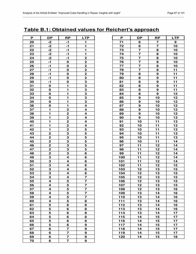
Analysis of the Article Entitled: “Improved Cube Handling in Races: Insights with Isight” Page 87 of 101 _________________________________________________________________________________________________________________
Table B.1: Obtained values for Reichert's approach
P DP RP LTP P DP RP LTP
20 -2 -1 1 71 6 7 9
21 -2 -1 1 72 6 7 10
22 -2 -1 1 73 7 8 10
23 -2 -1 1 74 7 8 10
24 -2 -1 2 75 7 8 10
25 -1 0 2 76 7 8 10
26 -1 0 2 77 7 8 10
27 -1 0 2 78 7 8 11
28 -1 0 2 79 8 9 11
29 -1 0 2 80 8 9 11
30 -1 0 3 81 8 9 11
31 0 1 3 82 8 9 11
32 0 1 3 83 8 9 11
33 0 1 3 84 8 9 12
34 0 1 3 85 9 10 12
35 0 1 3 86 9 10 12
36 0 1 4 87 9 10 12
37 1 2 4 88 9 10 12
38 1 2 4 89 9 10 12
39 1 2 4 90 9 10 13
40 1 2 4 91 10 11 13
41 1 2 4 92 10 11 13
42 1 2 5 93 10 11 13
43 2 3 5 94 10 11 13
44 2 3 5 95 10 11 13
45 2 3 5 96 10 11 14
46 2 3 5 97 11 12 14
47 2 3 5 98 11 12 14
48 2 3 6 99 11 12 14
49 3 4 6 100 11 12 14
50 3 4 6 101 11 12 14
51 3 4 6 102 11 12 15
52 3 4 6 103 12 13 15
53 3 4 6 104 12 13 15
54 3 4 7 105 12 13 15
55 4 5 7 106 12 13 15
56 4 5 7 107 12 13 15
57 4 5 7 108 12 13 16
58 4 5 7 109 13 14 16
59 4 5 7 110 13 14 16
60 4 5 8 111 13 14 16
61 5 6 8 112 13 14 16
62 5 6 8 113 13 14 16
63 5 6 8 114 13 14 17
64 5 6 8 115 14 15 17
65 5 6 8 116 14 15 17
66 5 6 9 117 14 15 17
67 6 7 9 118 14 15 17
68 6 7 9 119 14 15 17
69 6 7 9 120 14 15 18
70 6 7 9
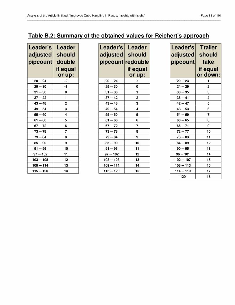
Analysis of the Article Entitled: “Improved Cube Handling in Races: Insights with Isight” Page 88 of 101 _________________________________________________________________________________________________________________
Table B.2: Summary of the obtained values for Reichert's approach
Leader's Leader Leader's Leader Leader's Trailer
adjusted should adjusted should adjusted should
pipcount double pipcount redouble pipcount take
if equal if equal if equalor up: or up: or down:
20 ─ 24 -2 20 ─ 24 -1 20 ─ 23 1
25 ─ 30 -1 25 ─ 30 0 24 ─ 29 2
31 ─ 36 0 31 ─ 36 1 30 ─ 35 3
37 ─ 42 1 37 ─ 42 2 36 ─ 41 4
43 ─ 48 2 43 ─ 48 3 42 ─ 47 5
49 ─ 54 3 49 ─ 54 4 48 ─ 53 6
55 ─ 60 4 55 ─ 60 5 54 ─ 59 7
61 ─ 66 5 61 ─ 66 6 60 ─ 65 8
67 ─ 72 6 67 ─ 72 7 66 ─ 71 9
73 ─ 78 7 73 ─ 78 8 72 ─ 77 10
79 ─ 84 8 79 ─ 84 9 78 ─ 83 11
85 ─ 90 9 85 ─ 90 10 84 ─ 89 12
91 ─ 96 10 91 ─ 96 11 90 ─ 95 13
97 ─ 102 11 97 ─ 102 12 96 ─ 101 14
103 ─ 108 12 103 ─ 108 13 102 ─ 107 15
109 ─ 114 13 109 ─ 114 14 108 ─ 113 16
115 ─ 120 14 115 ─ 120 15 114 ─ 119 17
120 18
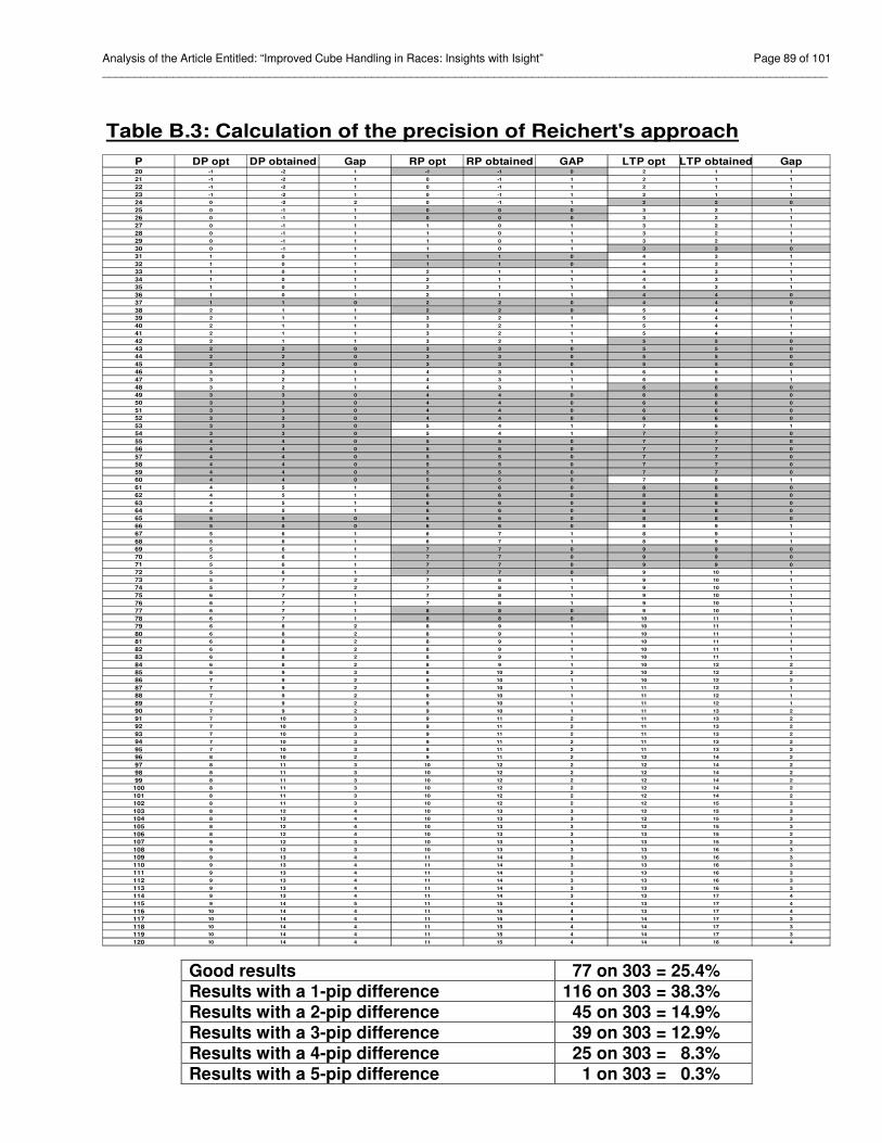
Analysis of the Article Entitled: “Improved Cube Handling in Races: Insights with Isight” Page 89 of 101 _________________________________________________________________________________________________________________
Table B.3: Calculation of the precision of Reichert's approach
P DP opt DP obtained Gap RP opt RP obtained GAP LTP opt LTP obtained Gap20 -1 -2 1 -1 -1 0 2 1 1
21 -1 -2 1 0 -1 1 2 1 1
22 -1 -2 1 0 -1 1 2 1 1
23 -1 -2 1 0 -1 1 2 1 1
24 0 -2 2 0 -1 1 2 2 0
25 0 -1 1 0 0 0 3 2 1
26 0 -1 1 0 0 0 3 2 1
27 0 -1 1 1 0 1 3 2 1
28 0 -1 1 1 0 1 3 2 1
29 0 -1 1 1 0 1 3 2 1
30 0 -1 1 1 0 1 3 3 0
31 1 0 1 1 1 0 4 3 1
32 1 0 1 1 1 0 4 3 1
33 1 0 1 2 1 1 4 3 1
34 1 0 1 2 1 1 4 3 1
35 1 0 1 2 1 1 4 3 1
36 1 0 1 2 1 1 4 4 0
37 1 1 0 2 2 0 4 4 0
38 2 1 1 2 2 0 5 4 1
39 2 1 1 3 2 1 5 4 1
40 2 1 1 3 2 1 5 4 1
41 2 1 1 3 2 1 5 4 1
42 2 1 1 3 2 1 5 5 0
43 2 2 0 3 3 0 5 5 0
44 2 2 0 3 3 0 5 5 0
45 2 2 0 3 3 0 5 5 0
46 3 2 1 4 3 1 6 5 1
47 3 2 1 4 3 1 6 5 1
48 3 2 1 4 3 1 6 6 0
49 3 3 0 4 4 0 6 6 0
50 3 3 0 4 4 0 6 6 0
51 3 3 0 4 4 0 6 6 0
52 3 3 0 4 4 0 6 6 0
53 3 3 0 5 4 1 7 6 1
54 3 3 0 5 4 1 7 7 0
55 4 4 0 5 5 0 7 7 0
56 4 4 0 5 5 0 7 7 0
57 4 4 0 5 5 0 7 7 0
58 4 4 0 5 5 0 7 7 0
59 4 4 0 5 5 0 7 7 0
60 4 4 0 5 5 0 7 8 1
61 4 5 1 6 6 0 8 8 0
62 4 5 1 6 6 0 8 8 0
63 4 5 1 6 6 0 8 8 0
64 4 5 1 6 6 0 8 8 0
65 5 5 0 6 6 0 8 8 0
66 5 5 0 6 6 0 8 9 1
67 5 6 1 6 7 1 8 9 1
68 5 6 1 6 7 1 8 9 1
69 5 6 1 7 7 0 9 9 0
70 5 6 1 7 7 0 9 9 0
71 5 6 1 7 7 0 9 9 0
72 5 6 1 7 7 0 9 10 1
73 5 7 2 7 8 1 9 10 1
74 5 7 2 7 8 1 9 10 1
75 6 7 1 7 8 1 9 10 1
76 6 7 1 7 8 1 9 10 1
77 6 7 1 8 8 0 9 10 1
78 6 7 1 8 8 0 10 11 1
79 6 8 2 8 9 1 10 11 1
80 6 8 2 8 9 1 10 11 1
81 6 8 2 8 9 1 10 11 1
82 6 8 2 8 9 1 10 11 1
83 6 8 2 8 9 1 10 11 1
84 6 8 2 8 9 1 10 12 2
85 6 9 3 8 10 2 10 12 2
86 7 9 2 9 10 1 10 12 2
87 7 9 2 9 10 1 11 12 1
88 7 9 2 9 10 1 11 12 1
89 7 9 2 9 10 1 11 12 1
90 7 9 2 9 10 1 11 13 2
91 7 10 3 9 11 2 11 13 2
92 7 10 3 9 11 2 11 13 2
93 7 10 3 9 11 2 11 13 2
94 7 10 3 9 11 2 11 13 2
95 7 10 3 9 11 2 11 13 2
96 8 10 2 9 11 2 12 14 2
97 8 11 3 10 12 2 12 14 2
98 8 11 3 10 12 2 12 14 2
99 8 11 3 10 12 2 12 14 2
100 8 11 3 10 12 2 12 14 2
101 8 11 3 10 12 2 12 14 2
102 8 11 3 10 12 2 12 15 3
103 8 12 4 10 13 3 12 15 3
104 8 12 4 10 13 3 12 15 3
105 8 12 4 10 13 3 12 15 3
106 8 12 4 10 13 3 13 15 2
107 9 12 3 10 13 3 13 15 2
108 9 12 3 10 13 3 13 16 3
109 9 13 4 11 14 3 13 16 3
110 9 13 4 11 14 3 13 16 3
111 9 13 4 11 14 3 13 16 3
112 9 13 4 11 14 3 13 16 3
113 9 13 4 11 14 3 13 16 3
114 9 13 4 11 14 3 13 17 4
115 9 14 5 11 15 4 13 17 4
116 10 14 4 11 15 4 13 17 4
117 10 14 4 11 15 4 14 17 3
118 10 14 4 11 15 4 14 17 3
119 10 14 4 11 15 4 14 17 3
120 10 14 4 11 15 4 14 18 4
Good results 77 on 303 = 25.4% Results with a 1-pip difference 116 on 303 = 38.3% Results with a 2-pip difference 45 on 303 = 14.9% Results with a 3-pip difference 39 on 303 = 12.9% Results with a 4-pip difference 25 on 303 = 8.3% Results with a 5-pip difference 1 on 303 = 0.3%
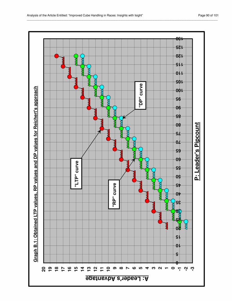
Analysis of the Article Entitled: “Improved Cube Handling in Races: Insights with Isight” Page 90 of 101 _________________________________________________________________________________________________________________
-3-2-10123456789
10
11
12
13
14
15
16
17
18
19
20
0
5
10
15
20
25
30
35
40
45
50
55
60
65
70
75
80
85
90
95
100
105
110
115
120
125
130
A: Leader's Advantage
P:
Le
ad
er'
s P
ipc
ou
nt
Gra
ph
B.1
: O
bta
ine
d L
TP
va
lue
s,
RP
va
lue
s a
nd
DP
va
lue
s f
or
Re
ich
ert
's a
pp
roa
ch
"LT
P"
cu
rve
"RP
" c
urv
e
"DP
" c
urv
e
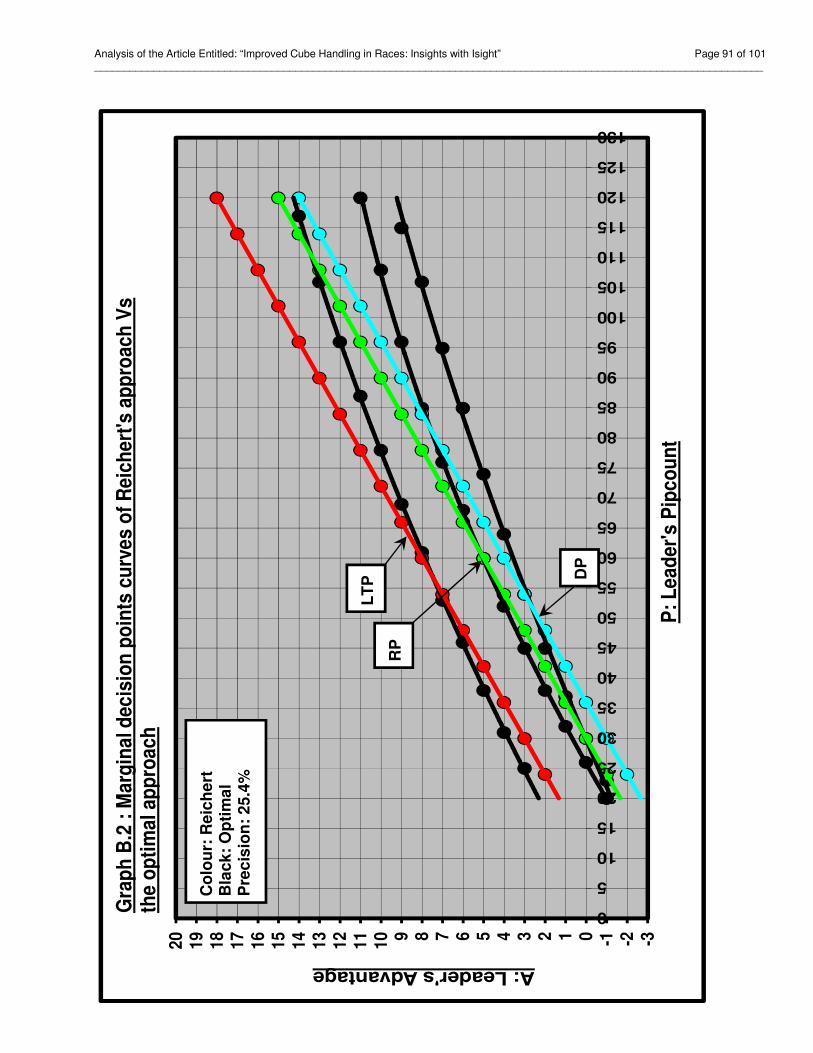
Analysis of the Article Entitled: “Improved Cube Handling in Races: Insights with Isight” Page 91 of 101 _________________________________________________________________________________________________________________
-3-2-101234567891
01
11
21
31
41
51
61
71
81
92
0
0
5
10
15
20
25
30
35
40
45
50
55
60
65
70
75
80
85
90
95
100
105
110
115
120
125
130
A: Leader's Advantage
P:
Le
ad
er'
s P
ipc
ou
nt
Gra
ph
B.2
: M
arg
inal d
ec
isio
n p
oin
ts c
urv
es o
f R
eic
hert
's a
pp
roach
Vs
th
e o
pti
mal ap
pro
ach
DP
RP
LT
P
Co
lou
r: R
eic
he
rt
Bla
ck
: O
pti
ma
l P
rec
isio
n:
25.4
%
Pre
cis
ion
: 4
1%

Analysis of the Article Entitled: “Improved Cube Handling in Races: Insights with Isight” Page 92 of 101 _________________________________________________________________________________________________________________
Appendix C: How to build a representative database The goal of this appendix is to clearly explain how to build a representative database and how to build a very representative database.
In this article, we have seen that:
• The “pip count adjustments” is defined as being all the adjustments to do in order to obtain an “adjusted” pip count.
• The “adjusted” pip count is obtained by calculating the “straight” pip count and by adding the “pip count adjustments”.
• The term “approach” is defined as being the decision criteria to follow in order to determine if a player should double or not, redouble or not, take or pass. So, an approach is to use three (3) mathematical formulas, namely:
o one (1) formula for the DP (Doubling Point); o one (1) formula for the RP (Redoubling Point); and, o one (1) formula for the LTP (Last Take Point).
• To apply an approach, it is necessary to calculate and to use the “adjusted” pip count of both players.
• The term “method” is defined as being the combination of a specific “pip count adjustments” associated with a specific “approach”. So in other words, we could say:
o method “A” is “A’s” pip count adjustments combined with “A’s” approach.
In order to obtain (or to develop) the best method, i.e. to obtain the best pip count adjustements and to obtain the best approach, it is necessary to use a database. Once this method is developed, it is necessary to use this method in order to obtain the adjusted pip count required to calculate the decision criteria, namely, the DP, RP and LTP. The term “data” is defined as being a single data. In the context of this article, a data is a specific backgammon position which could be identified and classified according these two following main features:
• The first main feature is race length.
• The second main feature is the wastage evaluation. The first main feature, i.e. the race length, is the leader’s pip count. Normally, the race length considered by an approach is from 20 pips to 120 pips.
Analysis of the Article Entitled: “Improved Cube Handling in Races: Insights with Isight” Page 93 of 101 _________________________________________________________________________________________________________________
The second main feature, i.e. the wastage evaluation, is the pip count adjustment to do to in order to obtain an adjusted pip count. When the race length is around 20 pips, the average wastage evaluation could be around 5.00 pips; and when the race length is around 120 pips, the average wastage evaluation could be around 1.00 pip. The term “database” is defined as being a data set. So, a database could contain a very high number of data. The expression “initial database” is defined as being the initial database which should contain all the available data possible to collect. The initial database must, among other things, contain the 50,000 data which are available at the following link: http://www.bkgm.com/articles/CubeHandlingInRaces/RaceDB.zip. The preceding link comes from Keith’s article. The initial database must also contain all others data that it is possible to collect. A “good database” is a database that contains several good data. A “good database” is not necessarily a “representative database”. Any database which only contains good data is necessarily a “good database” but it could very well be a “very unrepresentative database”. Theoretically, to use a database in order to obtain a reliable method, this database should necessarily be well weighed. To assess the quality of any database, it is necessary to assess it’s weighting. As a general framework, it is possible to classify any database as follow:
Type of database Main caracteristic Very unrepresentative Very poorly weighed Unrepresentative Poorly weighed Representative Well weighed Very representative Very well weighed
The use of an unrepresentative database will give an unreliable method. The use of an unreliable method will give inaccurate results. Because it is obvious that the initial database can not be well weighed, it implies that the initial database is an unrepresentative database. So, to obtain a reliable method, it is necessary to modify the initial database in order to get a representative one. To build a database considered as being representative, the number of theoretical values for each race length should be even. If the desired method wishes to accurately portray races from 20 pips to 120 pips, then, a representative database should contain the same number of data for each race length. That database should be built as follow:

Analysis of the Article Entitled: “Improved Cube Handling in Races: Insights with Isight” Page 94 of 101 _________________________________________________________________________________________________________________
• “n” data for 20 pips
• “n” data for 21 pips
• … • “n” data for 69 pips
• “n” data for 70 pips
• …
• “n” data for 119 pips • “n” data for 120 pips
From 20 pips to 120 pips, there are 101 pips. If “n” is 1, the database would contain 101 data. If “n” is 100, the database would contain 10,100 data. The higher the value of “n”, the more reliable the database becomes, the more reliable the developped method becomes, and the more accurate results get. In the context of this article, to obtain a representative database, a reliable method and accurate results; the minimum recommended “n” value is 100.
If a specific race length has less than “n” values, then, some data would have to be duplicated in order to get “n” values. For example, if at the specific race length of 120 pips, the number of known data in the initial database is 60 and the desired “n” is 100, then, it would be necessary to duplicate 40 data in order to get 100 values.
The use of a representative database should yeild a reliable method. The use of a reliable method should yeild accurate results. To obtain a database considered as very representative, it is necessary to assess the second main feature of each data, i.e. the wastage. To obtain a very representative database, it is necessary to modify the representive database obtained. To correctly assess the wastage, the theoretical criterion to respect is the following one: for each race length, the average wastage evaluation should correspond to the average wastage evaluation from the initial database. To obtain the average wastage evaluation for each race length from the initial database, it is necessary to use Reichert’s adjustments as presented in his article. The database will be very well weighed if, for each race length from 20 to 120, the average wastage evaluation is the average wastage evaluation from the initial database. Here are some examples:
• Example no 1: For the specific race length of 20 pips, the initial database contain 500 data and, in the initial database, the average wastage evaluation is 5.00 pips. So, for this specific race lengh, to obain a very representative database, the average wastage evaluation must be 5.00 pips.

Analysis of the Article Entitled: “Improved Cube Handling in Races: Insights with Isight” Page 95 of 101 _________________________________________________________________________________________________________________
• Example no 2: For the specific race length of 70 pips, the initial database contain 1,000 data and, in the initial database, the average wastage evaluation is 3.00 pips. So, for this specific race lengh, to obain a very representative database, the average wastage evaluation must be 3.00 pips.
• Example no 3: For the specific race length of 120 pips, the initial database contain 60 data and, in the initial database, the average wastage evaluation is 1.00 pip. So, for this specific race lengh, to obain a very representative database, the average wastage evaluation must be 1.00 pip.
The use of a very representative database will yeild a very reliable method. The use of a very reliable method will yeild very accurate results.
In summary we have:
Type of database Main
characteristic Main feature Obtained
method Obtained results
Very unrepresentative
Very poorly weighed
The theoretical values of the main feature (i.e. the race length) are not even at all
Is very unreliable
Is very inaccurate
Unrepresentative Poorly weighed
The theoretical values of the main feature (i.e. the race length) are slightly not even
Could be unreliable
Could be inaccurate
Representative Well weighed The theoretical values of the main feature (i.e. the race length) are even
Should be reliable
Should be accurate
Very representative
Very well weighed
The theoretical values of the main feature (i.e. the race length) are even, and the theoretical values of the second main feature (the average wastage’s evaluation) are well considered
Will be very reliable
Will be very accurate
In Keith’s article, Keith clearly mentioned that to compare the methods, he used real positions from real games. He also mentioned that “in this way, the types of positions which occur often in actual play are weighed more heavily than positions that happen only rarely.” Reichert analyzed Keith’s database and according to his results, the database used by Keith is a very unrepresentative database.

Analysis of the Article Entitled: “Improved Cube Handling in Races: Insights with Isight” Page 96 of 101 _________________________________________________________________________________________________________________
In Chabot’s article, it is clearly mentioned that Chabot’s approach is based on the optimal approach. The optimal approach is a very reliable approach because the database used to obtain it was a very representative database. Chabot’s approach indirectly uses the same database as for the optimal approach and that database is a very representative database.
In page 20 of his article, Reichert mentioned that he used Keith’s database. In pages 39 and 40 of his article, Reichert presented in figure 14 the distribution of race length in Keith’s database and noted that:
• About 50% of the race are shorter than 40 pips. • About 90% of the race are shorter than 70 pips.
• About 95% of the race are shorter than 75 pips.
A well weighed database should give the following results: • 50% of the race are shorter than 70 pips.
• 90% of the race are shorter than 110 pips.
• 95% of the race are shorter than 115 pips.
In summary, a well weighed database should have 50% of races shorter than 70 pips; while Keith’s database as used by Reichert has about 90% of races shorter than 70 pips.
It is very obvious that the database used by Reichert is a very unrepresentative database.
+ + + + +

Analysis of the Article Entitled: “Improved Cube Handling in Races: Insights with Isight” Page 97 of 101 _________________________________________________________________________________________________________________
Appendix D: Theoretical Money Proposition
Appendix D: DP valuesP Opt Chabot Gap Reichert Gap Money P Opt Chabot Gap Reichert Gap Money
(1) (2) (3) (4) (5) (6) (7) (1) (2) (3) (4) (5) (6) (7)
20 -1 0 1 -2 1 0 71 5 5 0 6 1 1
21 -1 0 1 -2 1 0 72 5 5 0 6 1 1
22 -1 0 1 -2 1 0 73 5 6 1 7 2 1
23 -1 0 1 -2 1 0 74 5 6 1 7 2 1
24 0 0 0 -2 2 1 75 6 6 0 7 1 1
25 0 0 0 -1 1 1 76 6 6 0 7 1 1
26 0 0 0 -1 1 1 77 6 6 0 7 1 1
27 0 0 0 -1 1 1 78 6 6 0 7 1 1
28 0 1 1 -1 1 0 79 6 6 0 8 2 1
29 0 1 1 -1 1 0 80 6 6 0 8 2 1
30 0 1 1 -1 1 0 81 6 6 0 8 2 1
31 1 1 0 0 1 1 82 6 7 1 8 2 1
32 1 1 0 0 1 1 83 6 7 1 8 2 1
33 1 1 0 0 1 1 84 6 7 1 8 2 1
34 1 1 0 0 1 1 85 6 7 1 9 3 1
35 1 1 0 0 1 1 86 7 7 0 9 2 1
36 1 1 0 0 1 1 87 7 7 0 9 2 1
37 1 2 1 1 0 -1 88 7 7 0 9 2 1
38 2 2 0 1 1 1 89 7 7 0 9 2 1
39 2 2 0 1 1 1 90 7 7 0 9 2 1
40 2 2 0 1 1 1 91 7 8 1 10 3 1
41 2 2 0 1 1 1 92 7 8 1 10 3 1
42 2 2 0 1 1 1 93 7 8 1 10 3 1
43 2 2 0 2 0 0 94 7 8 1 10 3 1
44 2 2 0 2 0 0 95 7 8 1 10 3 1
45 2 2 0 2 0 0 96 8 8 0 10 2 1
46 3 3 0 2 1 1 97 8 8 0 11 3 1
47 3 3 0 2 1 1 98 8 8 0 11 3 1
48 3 3 0 2 1 1 99 8 8 0 11 3 1
49 3 3 0 3 0 0 100 8 8 0 11 3 1
50 3 3 0 3 0 0 101 8 9 1 11 3 1
51 3 3 0 3 0 0 102 8 9 1 11 3 1
52 3 3 0 3 0 0 103 8 9 1 12 4 1
53 3 3 0 3 0 0 104 8 9 1 12 4 1
54 3 3 0 3 0 0 105 8 9 1 12 4 1
55 4 4 0 4 0 0 106 8 9 1 12 4 1
56 4 4 0 4 0 0 107 9 9 0 12 3 1
57 4 4 0 4 0 0 108 9 9 0 12 3 1
58 4 4 0 4 0 0 109 9 9 0 13 4 1
59 4 4 0 4 0 0 110 9 10 1 13 4 1
60 4 4 0 4 0 0 111 9 10 1 13 4 1
61 4 4 0 5 1 1 112 9 10 1 13 4 1
62 4 4 0 5 1 1 113 9 10 1 13 4 1
63 4 4 0 5 1 1 114 9 10 1 13 4 1
64 4 5 1 5 1 0 115 9 10 1 14 5 1
65 5 5 0 5 0 0 116 10 10 0 14 4 1
66 5 5 0 5 0 0 117 10 10 0 14 4 1
67 5 5 0 6 1 1 118 10 10 0 14 4 1
68 5 5 0 6 1 1 119 10 11 1 14 4 1
69 5 5 0 6 1 1 120 10 11 1 14 4 1
70 5 5 0 6 1 1
From 20 pips to 70 pips, Reichert's approach is pretty accurate
From 71 pips to 120 pips, Reichert's approach is very inaccurate
Legend Description
Result that counts toward the precision
Reichert's approach wins
No winnerChabot's approach wins
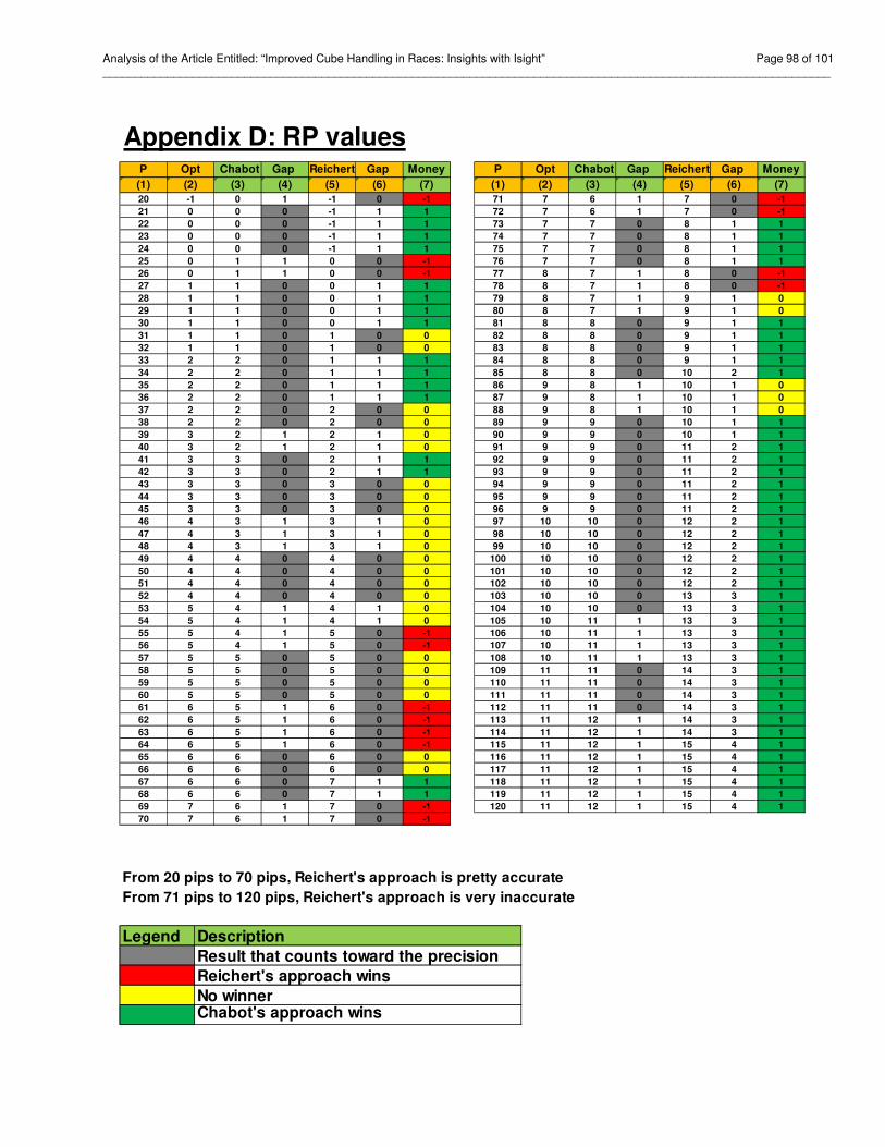
Analysis of the Article Entitled: “Improved Cube Handling in Races: Insights with Isight” Page 98 of 101 _________________________________________________________________________________________________________________
Appendix D: RP valuesP Opt Chabot Gap Reichert Gap Money P Opt Chabot Gap Reichert Gap Money
(1) (2) (3) (4) (5) (6) (7) (1) (2) (3) (4) (5) (6) (7)
20 -1 0 1 -1 0 -1 71 7 6 1 7 0 -1
21 0 0 0 -1 1 1 72 7 6 1 7 0 -1
22 0 0 0 -1 1 1 73 7 7 0 8 1 1
23 0 0 0 -1 1 1 74 7 7 0 8 1 1
24 0 0 0 -1 1 1 75 7 7 0 8 1 1
25 0 1 1 0 0 -1 76 7 7 0 8 1 1
26 0 1 1 0 0 -1 77 8 7 1 8 0 -1
27 1 1 0 0 1 1 78 8 7 1 8 0 -1
28 1 1 0 0 1 1 79 8 7 1 9 1 0
29 1 1 0 0 1 1 80 8 7 1 9 1 0
30 1 1 0 0 1 1 81 8 8 0 9 1 1
31 1 1 0 1 0 0 82 8 8 0 9 1 1
32 1 1 0 1 0 0 83 8 8 0 9 1 1
33 2 2 0 1 1 1 84 8 8 0 9 1 1
34 2 2 0 1 1 1 85 8 8 0 10 2 1
35 2 2 0 1 1 1 86 9 8 1 10 1 0
36 2 2 0 1 1 1 87 9 8 1 10 1 0
37 2 2 0 2 0 0 88 9 8 1 10 1 0
38 2 2 0 2 0 0 89 9 9 0 10 1 1
39 3 2 1 2 1 0 90 9 9 0 10 1 1
40 3 2 1 2 1 0 91 9 9 0 11 2 1
41 3 3 0 2 1 1 92 9 9 0 11 2 1
42 3 3 0 2 1 1 93 9 9 0 11 2 1
43 3 3 0 3 0 0 94 9 9 0 11 2 1
44 3 3 0 3 0 0 95 9 9 0 11 2 1
45 3 3 0 3 0 0 96 9 9 0 11 2 1
46 4 3 1 3 1 0 97 10 10 0 12 2 1
47 4 3 1 3 1 0 98 10 10 0 12 2 1
48 4 3 1 3 1 0 99 10 10 0 12 2 1
49 4 4 0 4 0 0 100 10 10 0 12 2 1
50 4 4 0 4 0 0 101 10 10 0 12 2 1
51 4 4 0 4 0 0 102 10 10 0 12 2 1
52 4 4 0 4 0 0 103 10 10 0 13 3 1
53 5 4 1 4 1 0 104 10 10 0 13 3 1
54 5 4 1 4 1 0 105 10 11 1 13 3 1
55 5 4 1 5 0 -1 106 10 11 1 13 3 1
56 5 4 1 5 0 -1 107 10 11 1 13 3 1
57 5 5 0 5 0 0 108 10 11 1 13 3 1
58 5 5 0 5 0 0 109 11 11 0 14 3 1
59 5 5 0 5 0 0 110 11 11 0 14 3 1
60 5 5 0 5 0 0 111 11 11 0 14 3 1
61 6 5 1 6 0 -1 112 11 11 0 14 3 1
62 6 5 1 6 0 -1 113 11 12 1 14 3 1
63 6 5 1 6 0 -1 114 11 12 1 14 3 1
64 6 5 1 6 0 -1 115 11 12 1 15 4 1
65 6 6 0 6 0 0 116 11 12 1 15 4 1
66 6 6 0 6 0 0 117 11 12 1 15 4 1
67 6 6 0 7 1 1 118 11 12 1 15 4 1
68 6 6 0 7 1 1 119 11 12 1 15 4 1
69 7 6 1 7 0 -1 120 11 12 1 15 4 1
70 7 6 1 7 0 -1
From 20 pips to 70 pips, Reichert's approach is pretty accurate
From 71 pips to 120 pips, Reichert's approach is very inaccurate
Legend Description
Result that counts toward the precision
Reichert's approach wins
No winnerChabot's approach wins
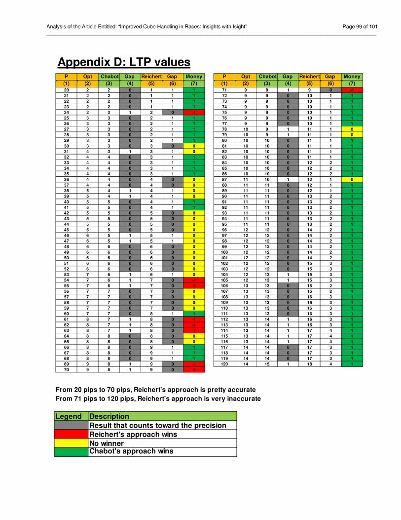
Analysis of the Article Entitled: “Improved Cube Handling in Races: Insights with Isight” Page 99 of 101 _________________________________________________________________________________________________________________
Appendix D: LTP valuesP Opt Chabot Gap Reichert Gap Money P Opt Chabot Gap Reichert Gap Money
(1) (2) (3) (4) (5) (6) (7) (1) (2) (3) (4) (5) (6) (7)
20 2 2 0 1 1 1 71 9 8 1 9 0 -1
21 2 2 0 1 1 1 72 9 9 0 10 1 1
22 2 2 0 1 1 1 73 9 9 0 10 1 1
23 2 2 0 1 1 1 74 9 9 0 10 1 1
24 2 3 1 2 0 -1 75 9 9 0 10 1 1
25 3 3 0 2 1 1 76 9 9 0 10 1 1
26 3 3 0 2 1 1 77 9 9 0 10 1 1
27 3 3 0 2 1 1 78 10 9 1 11 1 0
28 3 3 0 2 1 1 79 10 9 1 11 1 0
29 3 3 0 2 1 1 80 10 10 0 11 1 1
30 3 3 0 3 0 0 81 10 10 0 11 1 1
31 4 3 1 3 1 0 82 10 10 0 11 1 1
32 4 4 0 3 1 1 83 10 10 0 11 1 1
33 4 4 0 3 1 1 84 10 10 0 12 2 1
34 4 4 0 3 1 1 85 10 10 0 12 2 1
35 4 4 0 3 1 1 86 10 10 0 12 2 1
36 4 4 0 4 0 0 87 11 10 1 12 1 0
37 4 4 0 4 0 0 88 11 11 0 12 1 1
38 5 4 1 4 1 0 89 11 11 0 12 1 1
39 5 4 1 4 1 0 90 11 11 0 13 2 1
40 5 5 0 4 1 1 91 11 11 0 13 2 1
41 5 5 0 4 1 1 92 11 11 0 13 2 1
42 5 5 0 5 0 0 93 11 11 0 13 2 1
43 5 5 0 5 0 0 94 11 11 0 13 2 1
44 5 5 0 5 0 0 95 11 11 0 13 2 1
45 5 5 0 5 0 0 96 12 12 0 14 2 1
46 6 5 1 5 1 0 97 12 12 0 14 2 1
47 6 5 1 5 1 0 98 12 12 0 14 2 1
48 6 6 0 6 0 0 99 12 12 0 14 2 1
49 6 6 0 6 0 0 100 12 12 0 14 2 1
50 6 6 0 6 0 0 101 12 12 0 14 2 1
51 6 6 0 6 0 0 102 12 12 0 15 3 1
52 6 6 0 6 0 0 103 12 12 0 15 3 1
53 7 6 1 6 1 0 104 12 13 1 15 3 1
54 7 6 1 7 0 -1 105 12 13 1 15 3 1
55 7 6 1 7 0 -1 106 13 13 0 15 2 1
56 7 7 0 7 0 0 107 13 13 0 15 2 1
57 7 7 0 7 0 0 108 13 13 0 16 3 1
58 7 7 0 7 0 0 109 13 13 0 16 3 1
59 7 7 0 7 0 0 110 13 13 0 16 3 1
60 7 7 0 8 1 1 111 13 13 0 16 3 1
61 8 7 1 8 0 -1 112 13 14 1 16 3 1
62 8 7 1 8 0 -1 113 13 14 1 16 3 1
63 8 7 1 8 0 -1 114 13 14 1 17 4 1
64 8 8 0 8 0 0 115 13 14 1 17 4 1
65 8 8 0 8 0 0 116 13 14 1 17 4 1
66 8 8 0 9 1 1 117 14 14 0 17 3 1
67 8 8 0 9 1 1 118 14 14 0 17 3 1
68 8 8 0 9 1 1 119 14 14 0 17 3 1
69 9 8 1 9 0 -1 120 14 15 1 18 4 1
70 9 8 1 9 0 -1
From 20 pips to 70 pips, Reichert's approach is pretty accurate
From 71 pips to 120 pips, Reichert's approach is very inaccurate
Legend Description
Result that counts toward the precision
Reichert's approach wins
No winnerChabot's approach wins
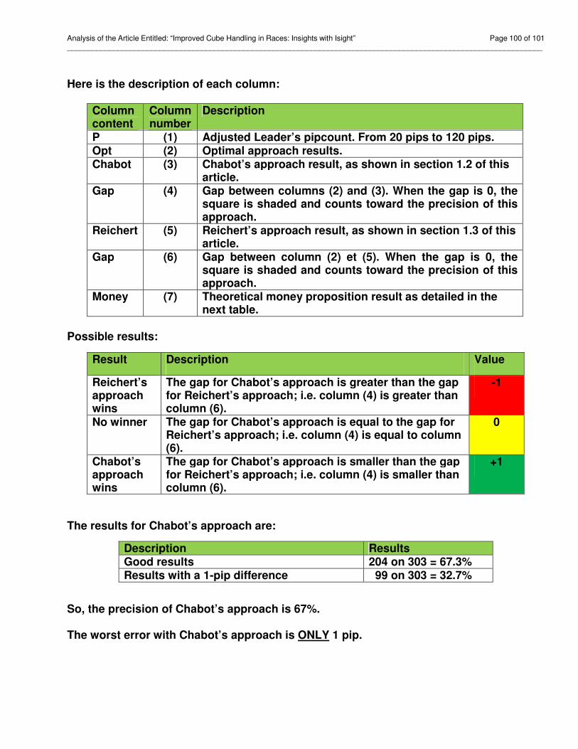
Analysis of the Article Entitled: “Improved Cube Handling in Races: Insights with Isight” Page 100 of 101 _________________________________________________________________________________________________________________
Here is the description of each column:
Column content
Column number
Description
P (1) Adjusted Leader’s pipcount. From 20 pips to 120 pips. Opt (2) Optimal approach results. Chabot (3) Chabot’s approach result, as shown in section 1.2 of this
article. Gap (4) Gap between columns (2) and (3). When the gap is 0, the
square is shaded and counts toward the precision of this approach.
Reichert (5) Reichert’s approach result, as shown in section 1.3 of this article.
Gap (6) Gap between column (2) et (5). When the gap is 0, the square is shaded and counts toward the precision of this approach.
Money (7) Theoretical money proposition result as detailed in the next table.
Possible results:
Result Description Value
Reichert’s approach wins
The gap for Chabot’s approach is greater than the gap for Reichert’s approach; i.e. column (4) is greater than column (6).
-1
No winner The gap for Chabot’s approach is equal to the gap for Reichert’s approach; i.e. column (4) is equal to column (6).
0
Chabot’s approach wins
The gap for Chabot’s approach is smaller than the gap for Reichert’s approach; i.e. column (4) is smaller than column (6).
+1
The results for Chabot’s approach are:
So, the precision of Chabot’s approach is 67%. The worst error with Chabot’s approach is ONLY 1 pip.
Description Results Good results 204 on 303 = 67.3% Results with a 1-pip difference 99 on 303 = 32.7%
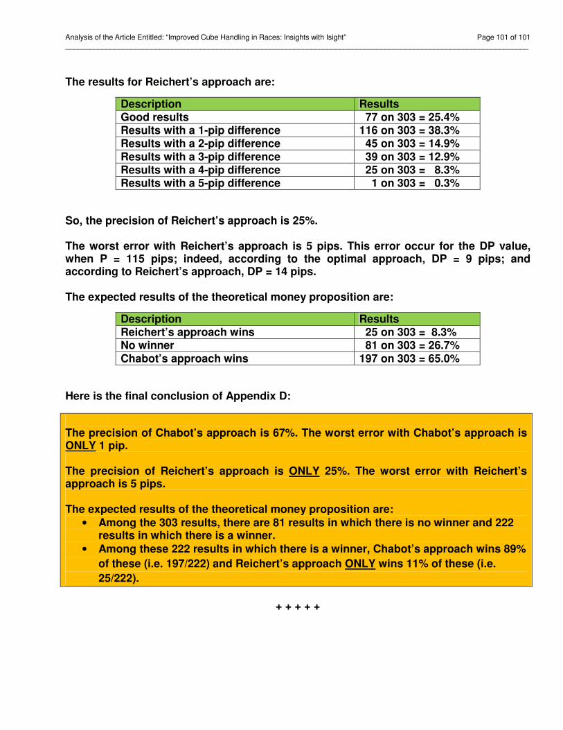
Analysis of the Article Entitled: “Improved Cube Handling in Races: Insights with Isight” Page 101 of 101 _________________________________________________________________________________________________________________
The results for Reichert’s approach are:
So, the precision of Reichert’s approach is 25%. The worst error with Reichert’s approach is 5 pips. This error occur for the DP value, when P = 115 pips; indeed, according to the optimal approach, DP = 9 pips; and according to Reichert’s approach, DP = 14 pips. The expected results of the theoretical money proposition are:
Here is the final conclusion of Appendix D:
The precision of Chabot’s approach is 67%. The worst error with Chabot’s approach is ONLY 1 pip. The precision of Reichert’s approach is ONLY 25%. The worst error with Reichert’s approach is 5 pips. The expected results of the theoretical money proposition are:
• Among the 303 results, there are 81 results in which there is no winner and 222 results in which there is a winner.
• Among these 222 results in which there is a winner, Chabot’s approach wins 89%
of these (i.e. 197/222) and Reichert’s approach ONLY wins 11% of these (i.e.
25/222).
+ + + + +
Description Results Good results 77 on 303 = 25.4% Results with a 1-pip difference 116 on 303 = 38.3% Results with a 2-pip difference 45 on 303 = 14.9% Results with a 3-pip difference 39 on 303 = 12.9% Results with a 4-pip difference 25 on 303 = 8.3% Results with a 5-pip difference 1 on 303 = 0.3%
Description Results Reichert’s approach wins 25 on 303 = 8.3% No winner 81 on 303 = 26.7% Chabot’s approach wins 197 on 303 = 65.0%