Analysis of the Computed Torque Drive Method and ... AERONAUTICS AND SPACE ADMINISTRATION Technical Memorandum 33-601 Analysis of the Computed Torque Drive Method and Comparison With

N A T I O N A L A E R O N A U T I C S A N D S P A C E A D M I N I S T R A T I O N

Technical Memorandum 33-601

Analysis of the Computed Torque Drive Method and

Comparison With Conventional Position Servo

for a Computer-Controlled Manipulator

B. R. Markiewicz

J E T P R O P U L S I O N L A B O R A T O R Y

C A L I F O R N I A INSTITUTE OF T E C H N O L O G Y

P A S A D E N A , C A L I F O R N I A

March 15, 1973

https://ntrs.nasa.gov/search.jsp?R=19730012471 2018-05-12T02:54:05+00:00Z

N A T I O N A L A E R O N A U T I C S A N D S P A C E A D M I N I S T R A T I O N

Technical Memorandum 33-601

Analysis of the Computed Torque Drive Method and

Comparison With Conventional Position Servo

for a Computer-Controlled Manipulator

B. R. Markiewicz

J E T P R O P U L S I O N L A B O R A T O R Y

C A L I F O R N I A INSTITUTE OF T E C H N O L O G Y

P A S A D E N A , C A L I F O R N I A

March 15, 1973

PREFACE

The work described in this report was performed by the Guidance and

Control Division of the Jet Propulsion Laboratory.

JPL Technical Memorandum 33-601 iii

CONTENTS

I. Introduction 1

II. Computed Torque System 1

1. Transfer Function Derivation 4

2. Response to Input Forcing Functions 13

3. Transfer Function for Feedback Position andRate Errors 13

4. Transfer Function for a Disturbance Torque 18

5. Feedback Gain Values and Resultant Response 20

III. Conventional Position Servo 24

1. Transfer Function Derivation 25

2. Stability Criterion 26

3. Response to Input Forcing Functions 28

4. Transfer Function for a Disturbance Torque. 32

5. Gain Values and Resultant Response 33

6. Effect of Changing System Inertia 36

IV. Comparison of the Two Drive Methods 37

Reference 40

Appendix A. Use of a Current Source for the Motor Drive 41

Appendix B. Effect of Manipulating a Large Inertia Object 45

Appendix C. Test for Maximum Motor Voltage 49

List of Symbols 51

FIGURES

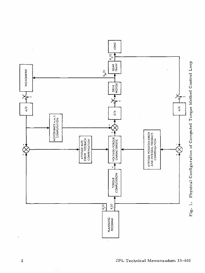
1. Physical Configuration of Computer Torque MethodControl Loop 2

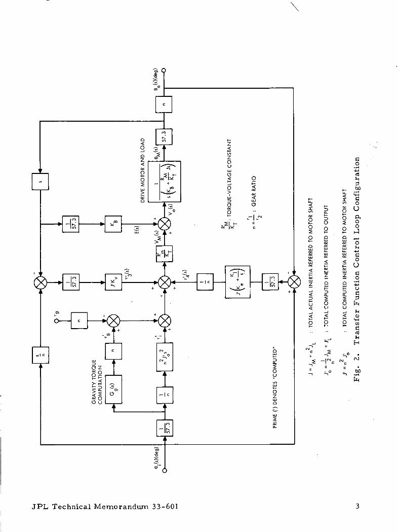
2. Transfer Function Control Loop Configuration 3

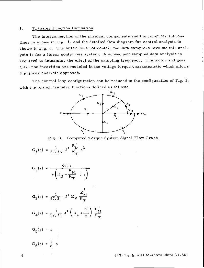
3. Computed Torque System Signal Flow Graph 4

JPL Technical Memorandum 33-601

CONTENTS (contd)

FIGURES (contd)

4. Typical Drive Motor Voltage — Torque Characteristic 10

5. Signal Flow Diagram for Position Feedback Null Error 14

6. Step Function Response for Unity Damping Ratio 16

7. Signal Flow Diagram for Rate Null Error 16

8. Signal Flow Diagram for a Disturbance Torque 18

9. Physical Configuration of a Control Loop 25

10. Transfer Function Control Loop Configuration 26

11. Typical Input Function, QJ(t) 29

VI JPL Technical Memorandum 33-601

ABSTRACT

A manipulator and its control system (modeled after a Stanford design)

is being developed at JPL as part of an artificial intelligence project. This

development includes an analytical study of the control system software.

This report presents a comparison of the computed torque method and the

conventional position servo. No conclusion is made as to the preference of

one system over the other, as it is dependent upon the application and the

results of a sampled data analysis.

JPL Technical Memorandum 33-601 vii

I. INTRODUCTION

A manipulator and its control system (modeled after a Stanford design)

is being developed at JPL as part of an Artificial Intelligence project. This

development includes an analytical study of the control system software. The

purpose of this report is to present the results of this study.

The Stanford manipulator control system models the manipulator and its

dynamics and computes the motor drive torque for each joint of the manipulator.

If the model •were exact, the manipulator could be driven open-loop with no

error. But because the model is not exact, rate and position feedback is used

in addition to the computed drive torque.

The manipulator operation is described from a. control analysis viewpoint

for the "Computed Torque" method in Section II and for a conventional position

servo in Section III. The gains and output response for both systems are

derived and discussed in detail. A comparison is made of the two control

methods in Section IV. The Stanford gain values are used here for the "Com-

puted Torque" method. But the final values may be different because the JPL

application does not require as high turning rates, and the design is slightly

different.

II. COMPUTED TORQUE SYSTEM

In the "Computed Torque" method the trajectory that the manipulator is

to follow as a function of time is computed in the planning program. Each

link angle, (the angle of the manipulator joint) as a function of time, necessary

to follow the desired trajectory, is also computed in the planning program.

The drive motor torque required to achieve the link angle/time function is

then computed based on a model of the manipulator hardware. The motor

voltage/torque characteristic is also modeled and the computed torque is con-

verted to applied motor voltage. This voltage is computed at a very high rate,

applied to D/A converter, and finally to the motor input.

If the manipulator and motor models •were exact, the response would be

exact, but this is not possible because of modeling inaccuracies and parameter

variations. Rate and position feedback is therefore used to compute correction

torques •which are summed with the main driving torque. The result is a sam-

pled data control system with performance dependent on the feedback gain values.

JPL, Technical Memorandum 33-601 1

oo

o

0)' O

U

VO

LT

AG

EC

HA

RA

CT

OR

QU

EC

OM

PU

TA

TIO

N

o

OG

RA

M

ot-t

•(->aoU

aoO

co

•H4->

«Jt-,SCuO&

OUr—4

rto

• iHtn>sAOH

h


asO

O

o

<

u<

oo

ou

ooso

ao

bo

ft

P Oa;LLJ £? o

I §o f^

o ^a

•• rt


1. Transfer Function Derivation

The interconnection of the physical components and the computer subrou-

tines is shown in Fig. 1, and the detailed flow diagram for control analysis is

shown in Fig. 2. The latter does not contain the data samplers because this anal-

ysis is for a linear continuous system. A subsequent sampled data analysis is

required to determine the effect of the sampling frequency. The motor and gear

train nonlinearities are modeled in the voltage torque characteristic which allows

the linear analysis approach.

The control loop configuration can be reduced to the configuration of Fig. 3,

with the branch transfer functions defined as follows:

Fig. 3. Computed Torque System Signal Flow Graph

G1<S ) =

R

KM 2

s

G 2 ( s ) = 57.3R

s K,, + MB K, J s

1 R1 j1 K —

57.3 J V KM

G4(s) = e s K

G 5 ( s ) = s

G6(s) = - s


G ? ( s ) = 1

Gg(s) = -1

K

G 0 ( s ) = 57.3

G1 0(s) = -1

Gn(s) = n

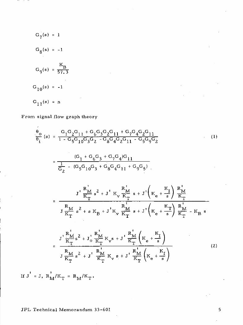
From signal flow graph theory

6.

G - ( G 5 G 10 G 3 + G 8 G 4 G 11 + G 9 G 5>

T . R M 2 , « K R M . T . / K , K I \ R M

J S +J K S + J K+—

R R' / K \ R1

M 2 __ i M , T i l v , Tl M77— s + s K^. + J K 77— s + J I K + J 77—KT B v KT \ e s / KT

R R1 R' / KT

RM 2 ^ • RM „ - T. RM [„ ^KlJ TT — s + J -r? — K s + J -=r — I K 4- —

Km Km v K^ \ e s

If J = J, RM /KT = RM /KT .

(2)

JPL, Technical Memorandum 33-601

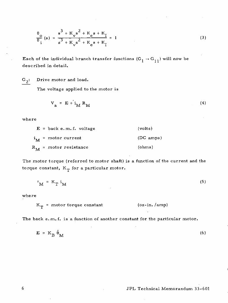
6 s3 + K s2 + K s + KT0 . . v e Ifi~ (s) = -o 5

1 s + K s + K s + KTv e l

Each of the individual branch transfer functions (G, —> G ' ) will now be

described in detail.

G-. Drive motor and load.

The voltage applied to the motor is

V = E + i,, R: (4)a M M

where

E = backe.m. f. voltage (volts)

i, . = motor current (DC amps)

R,., - motor resistance (ohms)

The motor torque (referred to motor shaft) is a function of the current and the

torque constant, KT for a particular motor.

TM - KT 4M (5)

where

KT = motor torque constant (oz-in. /amp)

The back e.m. f. is a function of another constant for the particular motor.

E = KB V (6)


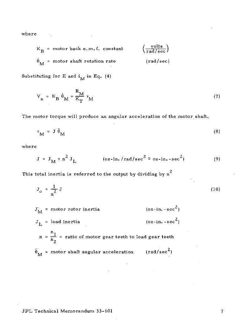
where

KT-. = motor back e. m. f. constant ( — v, / 1B \ rad/sec/

0 = motor shaft rotation rate (rad/sec)

Substituting for E and i in Eq. (4)

Va = KB °M + r TM

The motor torque will produce an angular acceleration of the motor shaft.

. . = j e.. (8)M M v

where

J = J, , + n J, (oz-in. /rad/sec = oz-in. -sec ) (9)JVL J-i

This total inertia is referred to the output by dividing by n

Jo = "T J

n

JM = motor rotor inertia (oz-in. -sec )

JT = load inertia (oz-in. -sec )J_j

nln = — - ratio of motor gear teeth to load gear teethn2

9 = motor shaft angular acceleration (rad/sec )

JPL. Technical Memorandum 33-601

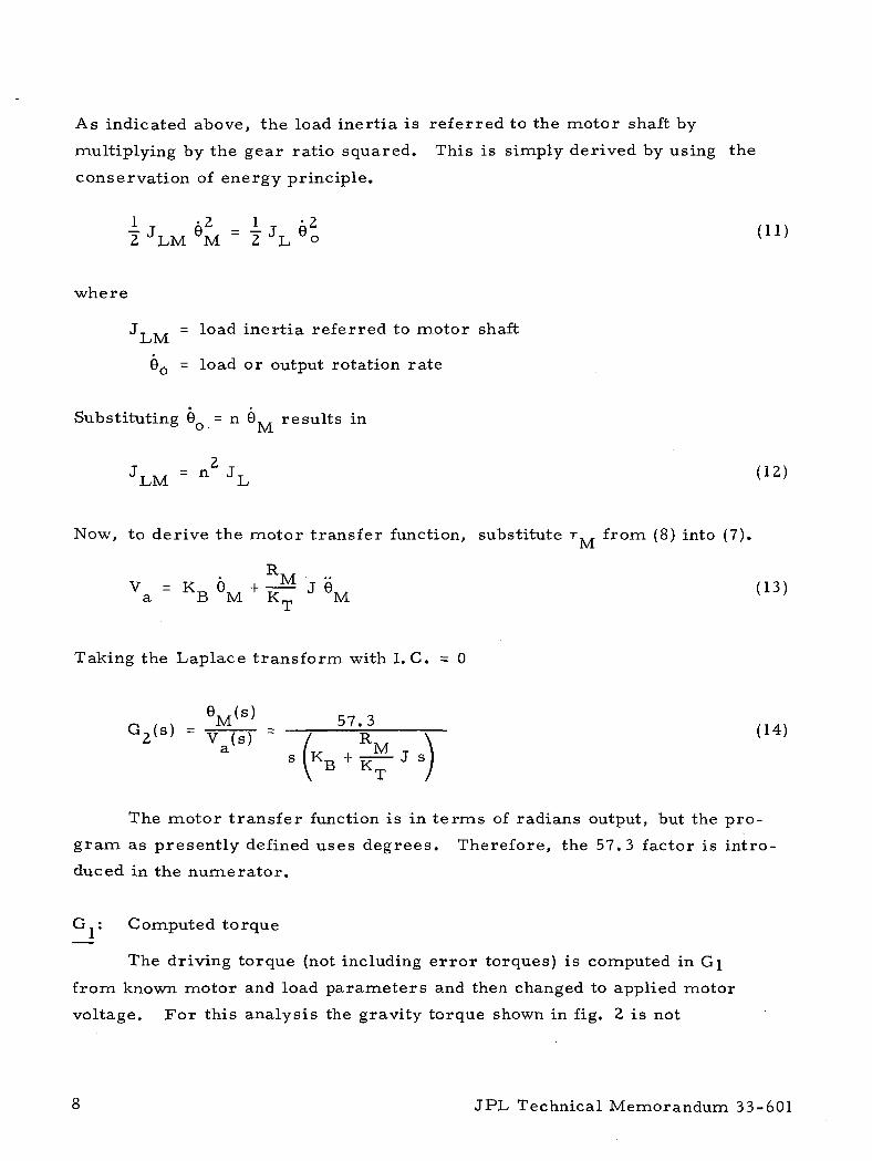
As indicated above, the load inertia is referred to the motor shaft by

multiplying by the gear ratio squared. This is simply derived by using the

conservation of energy principle.

I JLM *M = I JL 6o

where

JT .. , = load inertia referred to motor shaftLM

6^ = load or output rotation rate

Substituting 00 = n 0^ results in

Now, to derive the motor transfer function, substitute T from (8) into (7).

V. = 'KB *M + i? 'J 8M

Taking the Laplace transform with l.C. =0

57.3V (s) ~ / R_,a I,. , M T

S K + J

The motor transfer function is in terms of radians output, but the pro-

gram as presently defined uses degrees. Therefore, the 57.3 factor is intro

duced in the numerator.

G : Computed torque

The driving torque (not including error torques) is computed in G\

from known motor and load parameters and then changed to applied motor

voltage. For this analysis the gravity torque shown in fig. 2 is not

JPL, Technical Memorandum 33-601

included in G . This is done because it can be handled as a known disturbance1 i

input which is then cancelled by the computed gravity torque, T . As shown ino

Fig. 2 the gravity torque T is transferred from the output to the input for&

analysis purposes. It then has to be reduced by the gear ratio, n. The cancel-

lation can be quite accurate except for the effect of an unknown weight being

lifted by the manipulator, although the object weight can be determined from

the error signal and then included in the computed gravity torque. This will

be discussed under disturbance torque.

With the gravity loop eliminated, the remaining branch of G, computes

the required motor torque. From known manipulator parameters and 6.(t),

the changing inertia J (t) can be computed. Referring to Eq. (8), it is seen

that the torque is proportional to the angular acceleration and the total inertia

referred to the motor shaft. J (referred to output) is computed in the pro-

gram, therefore the n factor is needed. Angular acceleration can be computed

because 6.(t) is analytic (third degree polynomial) and is represented by s .

The 1/n factor is needed because 0^ refers to the manipulator joint angle, but

we are now referencing to the motor input. Therefore, Q: (used to compute

the motor torque) must be divided by the gear ratio. The final operation

here is to change this required torque to applied motor voltage. This could

be done as shown by using a constant R A , /K T (volts/oz-in.) which is the

torque to voltage conversion constant for a particular motor neglecting

motor friction and reduction gear losses. With only coulomb friction

torque present (given in motor specs), the constant slope voltage torque•

curve is displaced up for plus 0 by the voltage to overcome friction and

down for minus 9 . But with the reduction gear, the characteristics are not

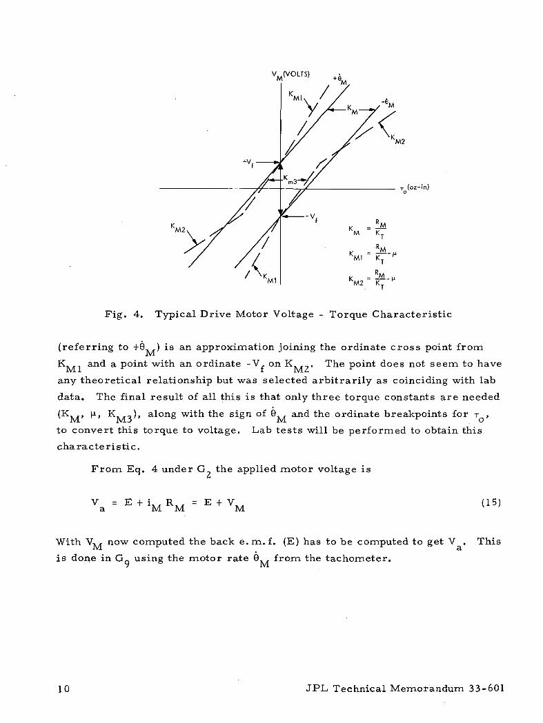
so simple. An approximation to the curves are shown in Fig. 4. They will

be determined from lab tests by measuring the output torque, keeping 9

constant and varying the applied voltage (the ordinate, V does not include the

back e.m. f. voltage). The solid lines are theoretical for no gear reduction

and the dotted lines connect data points from lab data. Note that there are

three different slopes or torque constants (K 1, K. ,?, K- _.,) . K 1 differs

from the theoretical value (Rj^/Kj) by the constant [i which is the additional

voltage required due to loss in the gear transmission. For + 9^ and +TO» (J. is

plus because the loss is opposing the desired output TQ, but for - TQ the loss

is aiding. The area covered by K , is somewhat nonlinear and the value K _


VM(VOLTS)

Fig. 4. Typical Drive Motor Voltage - Torque Characteristic

(referring to +0*,) is an approximation joining the ordinate cross point from

K, , and a point with an ordinate -V on K . The point does not seem to have

any theoretical relationship but was selected arbitrarily as coinciding with lab

data. The final result of all this is that only three torque constants are needed

(K , (J., K -), along with the sign of 0 and the ordinate breakpoints for T ,

to convert this torque to voltage. Lab tests will be performed to obtain this

characteristic.

From Eq. 4 under G the applied motor voltage is

V = E + i. . R. . - E + V. .a M M M

(15)

With VM now computed the back e.m. f. (E) has to be computed to get V . This

is done in Gn using the motor rate 9,. , from the tachometer.9 M

10 JPL Technical Memorandum 33-601

G/ ,G , - ,G i r . : Rate errorD D 1U

The motor output rate is obtained from the tachometer ( G _ ) mounted on

the motor shaft. The desired link angular rate (8.) is computed in the planning

program and is multiplied by 1/n to reference it to the motor. The two are

compared to indicate the rate error. The unity gain, G 1 f ) is only for transfer

function derivation purposes to separate the rate error from motor rate which

is used in G . The tachometer output is in volts, and an A/D converter is

required so the computer can interrogate the motor rate. The interrogation

of 0i is at some finite rate, thus, we have a. sampled data system.

G.,: Rate error feedback gain

The rate error is converted to radians/sec and multiplied by J to

remove this changing parameter from the system response characteristic.

If it remained, the damping ratio and natural frequency (reducing to a second

order system) would change with J . The system damping ratio is now a

function of the constant, K and of K .v e

G ,G0 : Position error< o

The manipulator link rotation angle (0O) is obtained from a potentiometer

mounted on the link, and the desired link angle (0.) is available from the planning

program. The two are compared to indicate the position error which is later

multiplied by 1/n to reference it to the motor. 0 is in volts, thus, an A/D

converter is required. As with 0 above, the interrogation is at some finite

rate, which makes the system a sampled data system which can be analyzed

as such using Z transform analysis methods. Any small delay time for reading

in 0^ and 0 can be incorporated in the analysis also.

G-: Position error and integral feedback gains

The position error is converted/to radians and multiplied by J as with

G.,, but here it is to keep the system undamped natural frequency constant.

The integral gain (KT) which will be discussed in Section II-4 is also now a

JPL Technical Memorandum 33-601 11

constant. It should be noted that the integration (K /s) is done numerically in

the computer as:

(1) Initialize T = 0

•where TJ^ is the computed torque for the present computation cycle

At is the computation cycle time

6£ is the position error in degrees

Gq: Motor back e. m. f. voltage

In Fig. 2 G^, G, and G . do not include the voltage -torque conversion

RV:

MM - IK.

because in the computer program, the three outputs are summed and only one

conversion is necessary. In the analysis the factor is included in each only for

simplicity, but the total output voltage is V (s).

From the G2 derivation, the applied motor voltage is

V = E + i. . RA, = E + V. ,a M M M

Thus, the back e.m.f. voltage, E has to be computed. This is done in G

in which the known motor constant K^ is used with the tachometer motorr>

rate.

E = ^ 6B o


2. Response to Input Forcing Functions

As shown in Eq. ( 3 ) the output is identical to the input if the inertia,t

J is computed correctly and if the voltage torque curve is exact,

i. e. ,

A .. \_ _M _ M

Therefore, the output or link movement 90(t) exactly follows the input, 6.(t)

which was computed in the planning program. But practically, errors due to

approximations in modeling and unknown system nonlinearities prevent this

ideal response, consequently the error feedback loops were included.

It is obvious that if the motor torque is computed correctly, the output

should respond correctly in an open loop manner and there would always be zero

error. And the previous derivation of the system transfer function would be

unnecessary. However, analyzing the response to disturbance torques or

unknown gravity torques does require a transfer function. Also, it is possible

to insert an inertia error, AJ and determine the response error. Additional

transfer functions are derived in the following sections.

3. Transfer Function for Feedback Position and Rate Errors

The two feedback transducers involved in each link control loop are a

potentiometer and a tachometer which could have bias or null errors. The

transfer functions for these errors can be derived easily from the system

transfer function derived in Section II-l.


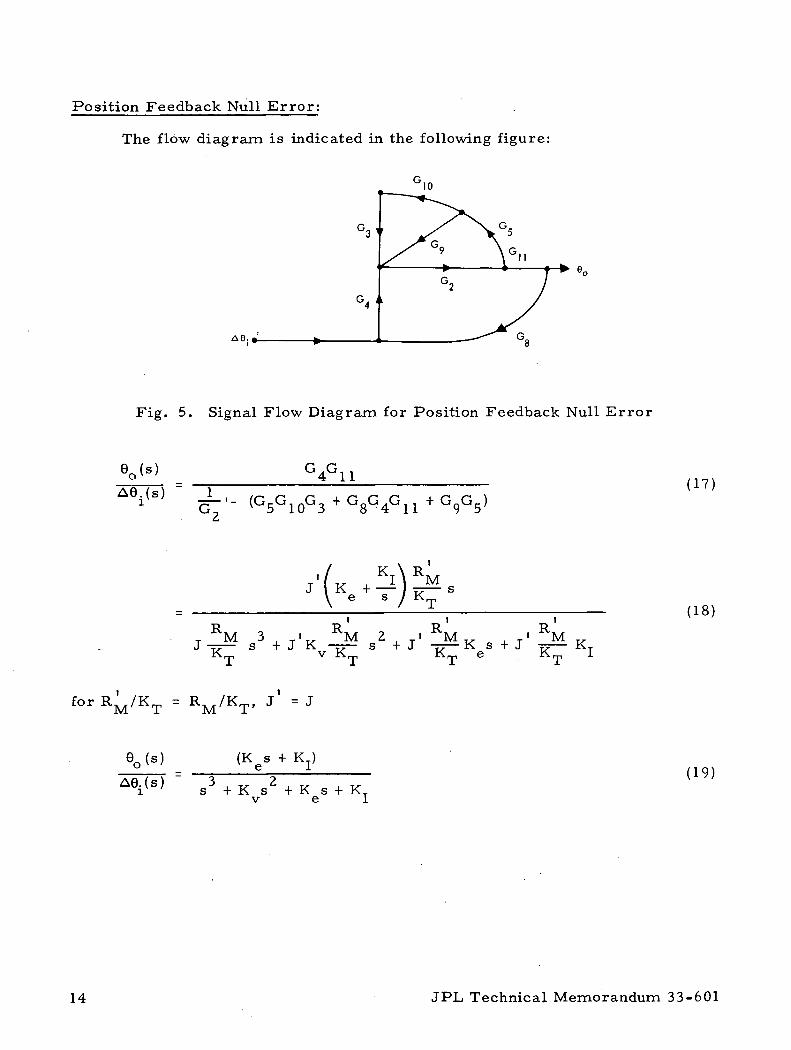
Position Feedback Null Error:

The flow diagram is indicated in the following figure:

10

11

Fig. 5. Signal Flow Diagram for Position Feedback Null Error

Vf>i

G4G11 (17)

J K + —\ e s

T M 3 . _ i _ _ M 2 , - i M „ . T ' M „J T?— s + J K -^— s + J -rr— K s + J -^— KTK v K K e K I

(18)

for RM /KT RM /KT , J = J

(Kes

s3 + K s2 + K s + KTv e I

(19)


ForAG.(s) = A G . / s

K (s + K /K )A6.6 ( s ) = 1 1—^ (20)

s(s + K s + K s + KT)v e I

The steady state error is

0o(t) = s 00(s) = A6. (21)

t -» co s -» 0

with KT = 0

K A6.60(s) = 2~^ l (22)

s(s + K s + K )v e

60(t) = A9. (23)

Thus, the steady state error is the same with or without the integral gain. The

second order transfer function can be in the form

A6. (s ) 2 - 2i s + 2t,oo s + wn n

(24)

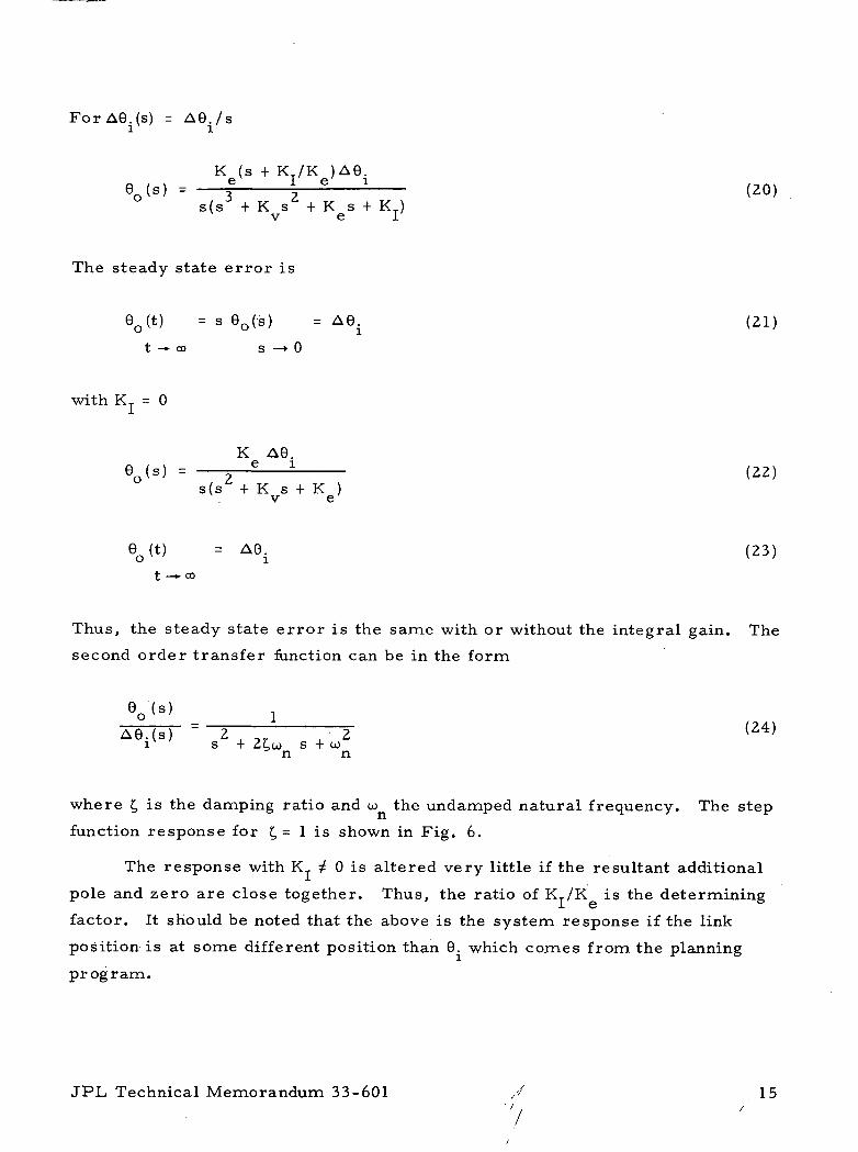
where t, is the damping ratio and w the undamped natural frequency. The step

function response for £, - I is shown in Fig. 6.

The response with K ^ 0 is altered very little if the resultant additional

pole and zero are close together. Thus, the ratio of KT /K is the determining

factor. It should be noted that the above is the system response if the link

position is at some different position than 6. which comes from the planning

program.

JPL Technical Memorandum 33-601 // 15• /

A8.

eo(0

t (SEC)

Fig. 6. Step Function Response for Unity Damping Ratio

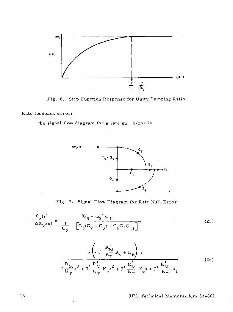
Rate feedback error:

The signal flow diagram for a rate null error is

Fig. 7. Signal Flow Diagram for Rate Null Error

eo(s)

- G,) +(25)

T RM 3 I RM v 2 , _i RM ... , _i RM „J T?— s + J -TT— K s + J -^— K s + J -37— KT

(26)


= J

Vs> ' \ ' "M

s3 + K s2 + K s + KTv e l

For a step input error, A0 (s) = AQ /s

for which

e0(t) = ot —» CO

If K = 0

n

for which

e ( s ) = -y =-^ ^ (28)s + K s + K s + KTv e l

6 n (s) = 5 ^ '- . (29)a (a + K s + K )v v e

iKT

Kv + R^Ke0(t) = —i K

M 00)t-*oo e

JPL Technical Memorandum 33-601 / 17

Thus, there is a steady state error if the integral feedback gain is zero. The

time required to bring this error to zero depends on the magnitude of K .

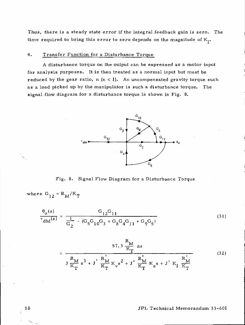
4. Transfer Function for a Disturbance Torque

A disturbance torque on the output can be expressed as a motor input

for analysis purposes. It is then treated as a normal input but must be

reduced by the gear ratio, n (n < 1). An uncompensated gravity torque such

as a load picked up by the manipulator is such a disturbance torque. The

signal flow diagram for a disturbance torque is shown in Fig. 8.

Fig. 8. Signal Flow Diagram for a Disturbance Torque

where

TdM ( s )

G12G11

G~ ~ (G5G10G3 + G8G4G11

(31)

c.-7 i57. 3 ns

I I I

, . M 3 , ' M T ^ 2 , T i M „ , T I T ^ MJ 77— s + J —— K s + J —— K s + J KT yr—

(32)


Since T ,. , = nrndM do

c_ _ 2 RMn . . 57.. 3 n —— s6 ( s ) Ku _ i (34)do R, , o i R, , -, , R.,. » RT. tj M83 ' M 2 « M • M

K KT v KT e KT I

For a step input, T , (s) = T , /s

eo(t) = o

with K = 0

,_ , 2 RM57. 3 n ^ — T ,K_ do90(t) = - 5 - i - (35)

The torque conversion factor was left in because in this case the R /K does

not cancel out if the computed value, R /K_ (from the curves) is not equal to

the real value, R., /K_ . If they are equal.M T ^

5 7 . 3 n 2 r9 (t) = - i - 2£_ (36)

J Kt— •-« e

where T is the disturbance torque in oz-in. , and 6Q is in degrees.

As might be expected, the steady state error is not a function of the

changing inertia (J), but with the J multiplier the error is reduced by thei

resultant gain, J K .


5. Feedback Gain Values and Resultant Response

The purpose of this section is to insert gain values in the various transfer

functions and steady state error expressions to indicate realistic output error

values. The gains used are the Stanford values but will be converted to»'*

eliminate the At (jiffy)'1" element. This is necessary to use them in the transfer

functions.

First, we will look at the characteristic equation.

s3 + K s2 + K s + KT = 0 (37)v e I v '

If K, = 0, we have

s2 + K s + K =0 (38)v e

which is a second order system and can be expressed as

s2 + 2£w s + w2 = 0 (39)

in which

C = the system damping ratio

to = the system undamped natural frequency (rad/sec)

Common practice is to select £= 0. 7 and w as high as practical to

increase the response or tightness of the servo loop. Stanford has selected

£ = 1 which is reasonable since the overshoot for a step input is then reduced

from 7% (£, = 0. 7) to zero. Doing this we have

2u = K in v

w2 = Kn e

^The term "jiffy" refers to the 1/60 second sampling interval used at Stanford.


or

- \2

Ke = V-TV/ <40>

Now. selection of K or K determines co . Remember from Fie. 6 that the' e v n & _

response has reached its final value (practically speaking) at t = 7 /w = 7/ v K .jfl C

This is all very nice, but as shown above the characteristic with

K 1 0 is third order. Fortunately, (depending on the value of K ) the system

can still be considered second order to get a measure of the system transient

response. This will be elaborated upon further.

The gains used by Stanford for joint 1 are

K = 0.038e

K = 0. 39 (41)

K = 0. 005

These have the time element of 1/60 sec in them, therefore to eliminate this,

K = 0.39 x 60 = 24.4

K = 0.038 x 602 = 132 . (42)G

K. = 0.005 x 603 = 1080

Substituting these values in the transfer function for a step displacement from

E q . 1 9 . . .

_ _A6i(s) s3 + 24s2 + 132s + 1080

(43)


factoring (for Stanford gains)

132(s + 8)A6i(s) (s + 20 .2 ) ( s 2 + 3.9s + 52)

= 1080

= 0. 27

co = 7 . 2n

(44)

If K is doubled

I32(s + 16.3)A6i(s) (s + 22.4)(s 2 + 1.6s + 96)

f K = 216U

t, = 0.08

co = 9 . 8n

(45)

for KT = 0

Ae.(s)K

s + 24.4s + 132CO n

= 0

= 1.0

= 11.5

(46)

As K, increases from 0—- 1080 the transient response is altered very

little (althoughithe steady state error will now go to zero over a longer time

than the initial transient). At K,. = 1080 the zero and pole added are not too

close together, the t, is quite low, but the pole has a stabilizing effect to cancel

the destabilizing effect of the zero and the decreased £,. The result is a response

similar to when K, = 0. But as K approaches 2160, the pole and zero approach

each other and can be cancelled leaving just a second order system with very

low damping. As K increases further the system becomes marginally stable,

i. e. , t, = 0. Thus K cannot be increased much beyond 1000.

For stability purposes KT has to be controlled as above, but to eliminate

rate and position null errors and to reduce the output from a torque disturbance


to zero as rapidly as possible, K, should be large as feasible. The restriction

for at least marginal stability is that

KI £ KvKe <47'

This is derived from the characteristic equation in Eq. (19). Let K, = K K in^ I v e

s3 + K s2 + K s + KT = 0v e l

which then factors into

(s + KV) (s2 + Kg) = 0

This indicates that the two complex roots are on the imaginary axis of the

complex s plane, therefore the system is marginally stable.

If K and K are selected on the basis of considering only the second orderv G

response for ^ = 1 (Eq. 40), then

The above restriction on KT applies as well to a torque disturbance since the

characteristic equation (Eq. 34) is the same. It is of some interest to consider

the steady state error when KT = 0.

57.3 n2 T,6o (*) = - T - - (49)

J Kt— *• oo e

In all the previous discussion the value of J did not matter since it cancels

out if all gains and operations are as shown in Fig. 2. Here we have assumed

that J not J is used as the gain multiplier, otherwise the n factors would be

different. Consequently, the above error is a function of J , the computed2 l:

inertia referred to the motor. This is of course n JQ.i

A value of J for the first link from the Stanford arm is derived as

follows (the prime denoting computed is dropped).

2T

2r

Load inertia: J = 413,000 oz-in. jiffy\-iO


Total inertia: JQ = 698,000 oz-in. jiffy

Motor inertia: J.., = 285,000 oz-in. jiffy'

To eliminate the jiffy time element requires dividing by 60

JT = 115 oz-in.-secLo

J =79 oz-in.-secMo

The total inertia referred to the motor is

J = nZ(J. / r + JT ) (50)Mo Lo

1 (79 + 115)(120)2

= 0.005 + 0.008 = 0.013 oz-in. sec

The value of n for the JPL arm (link 1) is 100 and the inertia values •will be

larger.

Substituting values in (49)

57.3 T,60(t) = = — = 0.002 T (51)

(120) (0. 013)(132)t —*-co

If a force of 16 oz is applied with a lever arm of 30 inches, the resulting output

angular error is 0. 96 degrees. Thus if this magnitude of error cannot be

tolerated, K -would have to be increased, keeping in mind that J is a variable.

The other alternative is to introduce the integral gain, K which would reduce

the error to zero.

III. CONVENTIONAL POSITION SERVO

The positional servo described here uses the same sensors or trans-

ducers as the computed torque system but feeds this information directly

to a summing amplifier which drives the motor, rather than to the computer.


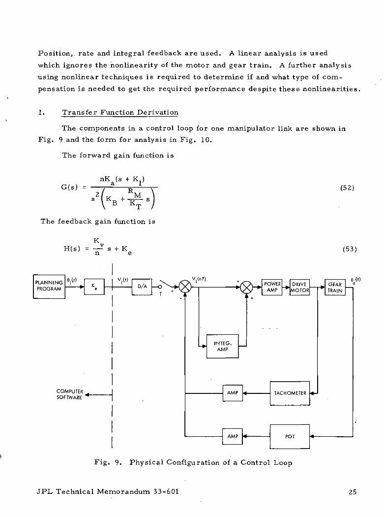
Position, rate and integral feedback are used. A linear analysis is used

which ignores the nonlinearity of the motor and gear train. A further analysis

using nonlinear techniques is required to determine if and what type of com-

pensation is needed to get the required performance despite these nonlinearities,

1. Transfer Function Derivation

The components in a control loop for one manipulator link are shown in

Fig. 9 and the form for analysis in Fig. 10.

The forward gain function is

G(s) =nK (s + K )

Cl J_

The feedback gain function is

KH(s) = —- s + K

PLANNINGPROGRAM

6jWK

v.WD/A h-O

T

COMPUTERSOFTWARE '

(52)

(53)

V.(nT)GEARTRAIN

6(0o

Fig. 9. Physical Configuration of a Control Loop


e.(s)

(RAD)

V.(nT)

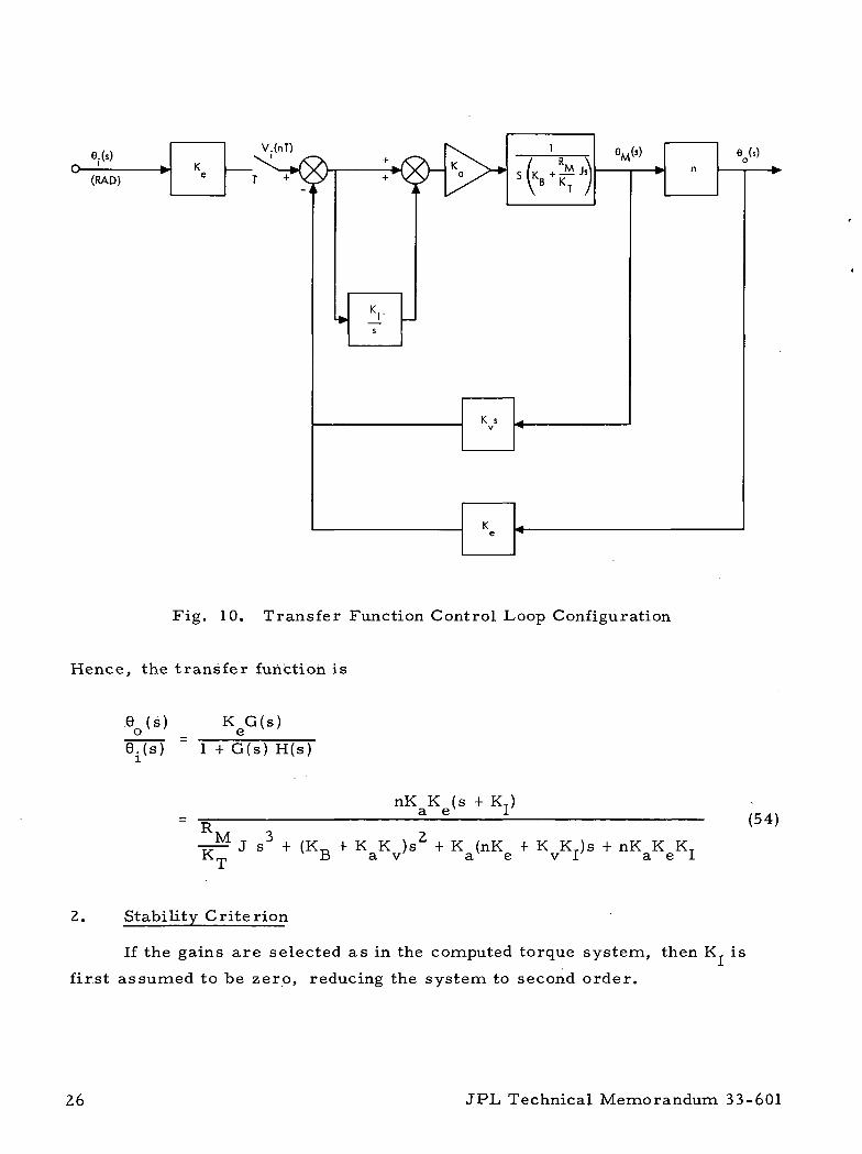
Fig. 10. Transfer Function Control Loop Configuration

Hence, the transfer function is

Vs)6.(s)

K G(s )

G(s) H(s)

nK K (s + KT)a e ITJ

J s3 + (K^ + K K )s2 + K (nK + K KT)s + nK K KTv B a v' av e v I a e I

(54)

2. Stability Criterion

If the gains are selected as in the computed torque system, then K is

first assumed to be zero, reducing the system to second order.


a i \ nK K / J V1

6Q (s) a e/ KT

6 . ( s ) = ~ ( K n + K K ) n K K (55)

i 2 , B a v , a eS + p- S + j£

T M T MKT KT

where

R,w = In K K /JTT^ (56)n V a e/ ^ ' x

+ K K(57)

R l/20 i T » T , T2 I nK K J

a e

selecting t, = 1 and solving for K and Kct v

R. . R , R- K^K + 2nK J-r ±2 nK J rr nK J - ^

B v e K J e KT \ e K B v/K = - - ± - 1-_ - L-± - L_ - /_ (58)

v

KB + Z

(59)

In the above equations, all parameters except K are known, and a maximumG

value for this gain will be developed in Section 5.

From Eqs. 27, 47 and 54 the stability criterion with KT ^ 0 is

nK K KT K (K_. + K K )(nK + K KT)V I < -a-5 - 1^_^ — v_^_ (60)

KT


or

nK (K^ + K K )5 R

e B Su_v

n J K Ke - Kv<KB + KaKv)

Generally the second denominator term is very small and

K^ + K KK < B a v (62)

J MJ

This criterion only specifies a maximum K for conditional stability. Of

course K and K did not have to be computed from Eqs. 58 and 59 for t, = 1

but that is a preferable way. The point to consider is the proper value of

K « K to produce a transient response similar to that expected from

the second order equation.

3. Response to Input Forcing Functions

The response to an input from the planning program, unlike the com-

puted torque case, depends entirely on the feedback gains. The input is 6.(t)

and the ability of 6o(t) to follow depends on the amplification of the resultant

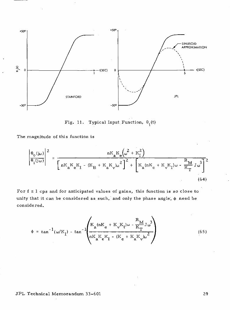
error signal which then drives the motor. A typical input function is shown

in Fig. 11. As indicated the JPL requirement is for a slower response,

at least for the present.

A measure of the error in 9o(t) can be obtained by approximating the

input function with a sinusoid as shown, and then finding the frequency response

to this input frequency, w.

Substituting jco for s in Eq. (54).

60(>>) n K K ( j U + K )- a e

e.(j«) -nKaKeKI - ^B + ̂ V^ + K[K (nK + K KT)w - -^ w3

av e v I' KT


+50°

"• 0

-50°

+50°

STANFORD

-) t(SEC) 01

-50°

SINUSOIDAPPROXIMATION

t(SEC)

JPL

Fig. 11. Typical Input Function, 6.(t)

The magnitude of this function is

1

2 v v ( 2 , ^2\nK K i r . ) + Kr 1a e\ I /

nPC PC PC _ /PC - I - P C P C V > 4- PC fnPC 4 PC PC ^

RM 31 2

a v...

a e

(64)

For f < 1 cps and for anticipated values of gains, this function is so close to

unity that it can be considered as such, and only the phase angle, 4> need be

considered.

<j> = tan (co/KT) - tan

RK (nK + K KT)u> -

If a e v T T

InK K KT - (K + K K1 a e I e a. v

(65)


For f = 0.2 (co = 1.356), K^ = 0.001, K& = 200, KB = 0.05, J = 0.013,

R,. , /K^ = 0. 123, which are nominal values, this reduces toM 1

4> = tan - tan"1 K KT

v

nK

4> = tan-1 -co K

v I

nK co'2K KTv I

for K » co (Kj. * 10)

<f> = tan. . - co K K

-1 f v I

nK KT + co Ke l v

For n = 0.01, Kg = 7,

values,

= 10, K = 0.001, w = 1.356, which are nominal

, .* = - tan

/xaKv (rad) (66)e

This is the phase lag in 6_( t ) for a sinusoidal input, 6.(t)

error in 6 (t) can be expressed as

sin cot. The

A 6 ( t ) = - 0 sin cot + 6 sin (cot + $), s neg.

= 9 [ sin cot (cos <f> - 1) + cos cot sin (67)

For small cj>

A60(t) = 6 $ cos cot (68)


where

6 is the peak angular sinusoidal rotation

cf> is the phase lag in radians from Eq. (66).

Another way of determining the response error is to assume a ramp

input for 6.(t).

e.(t) - kt - (69)

From Eq. (55) for t, - 1, we have

e . ( s ) sz 2 se.(T- + S + 12 wu> nn

Therefore

e ( s ) = ko 2

*'1

*in J60(t) = k l - (1 + W t ) e (72)


The output error is

A6n(t)f * [e.(t) - eo(t)]

Jodt

= ko / -W t

of I 1 ' 6 n

-u) t-t e (73)

where w can be computed from the system parameters, and k is the ramp slope

in degrees or radians per second.

4. Transfer Function for a Disturbance Torque

An output disturbance torque, T can be transferred to the motor input

by multiplying it by the gear ratio.

TdM = n Tdo(74)

Therefore, applying rj*A at the motor input

G(s) =n

(75)

T .

/ K KH(s) = K IK +—- s + —a \ e n s (76)

RM

Kn G(s )

+ G ( s ) H ( s )

R

KM 2n s

TJ

Js3 +

(77)

^ + K K )s + nK K s + nK KTB a. v a e a I


For a step disturbance torque, the output error is

™M T , nK 'doeo(s) = -^ (78)

-r^ Js3 + (K^ + K K )s2 + nK K s + nK KT. Krr, B a v a e a I

The steady state output error is

eo(t) = s e0(s) = ot-*-co s— ̂ 0

5. Gain Values and Resultant Response

The determination of gains for this system is more complicated than for

the computed torque system since more variables are involved and physical

limitations come into play. Selecting gains based on a second order response

as mentioned before means arbitrarily letting the damping ratio, £ = 1, and

selecting'an arbitrary undamped natural frequency, w . The latter can be done

by considering the response desired as shown in Fig. 6.

The equations for the gains ( £ = 1 ) are

Kv - Rn

n

Ka =

Nominal values of the above parameters are

J = 0. 013 (oz-in. sec )

RM/KT = 0.123 (v/oz-in. ) (81)

KB = 0.05 (v/rad/sec)

n = 0.01 ( N / N 2 ) gear ratio


The value of K is dependent on the angular range which is ±180° and the supply

voltage = 24. Thus, the pot sensitivity is ±12/ir (volts/rad). Adding some

amplification -with the same D.C. voltage supply can increase this to±24/ir . A

value of K = 7 will be used here. Inserting all these values in (79) and (80).

K = i Z- (82)V w

K = 0.023 wa n

Selecting to = 100 for a very fast step response (Fig. 6).

K = 0.0012v

K = 230a

(83)

Now K, has to be selected

K + K KKT < * p

a v = 204 (84)i K-T. ,

T M

KT

Obviously, to get a response approaching £, = 1, KT has to be considerably

less than this maximum value. Selecting K = 10, the system transfer function

is:

6o(s) _ 10, 062(s + 10)ei(s) s3 + 203.7s2 + 11, 787s + 100, 625

Factoring

6o (s) 10,062(s + 10)2

(s + 10. 2)(s + 193.5s + 9813)

,.( '


Obviously, the pole and zero essentially cancel and the response is second

order with

"n(86)

£ = 0.98

The high values of K and K and the relatively low KT has left the responseV cL -L

the same as without KT. This is fine except that high amplifier gains create

a noise problem. The transient response is much better than needed, but

to control the error for a very rapidly changing input forcing function such as

shown in Fig. 11, requires a high gain. From the sinusoidal input error func-

tion (Eq. 68) and Eq. 66,

A6 (t) = 9 4> cos wto p

cos ait (87)

Substituting the previously given parameter values

A6o(t) = 6 tan"1(0. 017w) cos wt (88)

For 6 = 50 deg, co= 1.356

A9Q = 50(0.023) = 1. 15 degrees (89)

For w = 6. 28 which is a nominal input for the computed torque system at

Stanford, this error increases to 5 degrees. Thus, it is obvious that, if the

system is to compete with the Stanford computed torque system, the gains

would have to be increased which is feasible.


A check on the above response error is to use error Eq. (73) for a ramp

input. For the sinusoid used, the maximum 6 is about 60 deg/sec. The

natural frequency from Eq. (86) is 100 rad/sec.

[ 7 / ~ui,,t ^ "^r,1- 1f ( l - e n ) -t e n

n J

(90)

Thus, for t > 0. 1 seconds, the error equation reduces to

?!<•A60 = = 1. 2 degrees (91)

n

which compares well with the previous value of 1. 15 degrees from (89).

6. Effect of Changing System Inertia

The inertia changes as the manipulator moves links which extend or

retract the arm. This is of no consequence for the computed torque system

since it is computed and the computed value is used to eliminate this parameter

from the system response. This is essentially computing a variable feedback

gain. For the conventional system the natural frequency and damping are

(92)

K^ + K KY _ B a v

2 nK K J


As discussed, this is the case if the gains are as shown earlier which

essentially reduces the system to second order.

The inertias of the JPL arm are not yet known. They will be larger

than the Stanford values which have been used in this report, but using Stanford

values is most likely sufficient for this discussion. Supplied data indicates

that the inertia value can about double for link No. 1. This means w and £, arendecreased by ^Z~which would not change the transient performance or decrease

the stability any significant amount. This is even less significant for other

links, except when a large inertia object is being manipulated.

IV. COMPARISON OF THE TWO DRIVE METHODS

The following paragraphs are a summary of the more important character-

istics of the computed torque (CT) and conventional position servo (CS) systems.

However, no final conclusion is made as to which system should be used because

this depends on the particular application and on the results of a sampled data

analysis.

1) Input Forcing Functions

CT: There is theoretically no output position error if the torque is

computed correctly to produce the response computed in the plan-

ning program. This assumes the inertias are computed correctly.

The advantage here is that very fast motions can be accomplished

without depending on a feedback error.

CS: There is always a transient error which subsides to zero as

the motion rate decreases to zero. This error is minimized by

selecting the largest possible forward and feedback gains.

2) Disturbance Torque

CT: An unknown external force on the manipulator is a disturbance

torque. Gravity torques are computed and compensated along with

reaction torques from rotations in other non-perpendicular links.

Lifting an object produces an unknown torque which results in an

angular position error. The integral gain term then zeros this

position error due to any unknown torque. The resulting output

of the integral gain term indicates the torque value and thus the

weight of the object.


CS: The feedback error signal from the integrating amplifier must

compensate for all disturbance torques including gravity and

reactions from other links. This is not too serious a problem with

high enough gains. The reaction torques are only about 5% of the

applied torque, and the gravity torques would not pose any problem

since the output error is driven to zero by the integral term. Very

fast motions with a large changing gravity and reaction torque

would produce an error dependent on the gain values.

3) Gains

CT: The feedback gains (link 1) are such to produce a damping ratio

(£,) of 1 and an undamped natural frequency of about 10. This is

not a very tight loop, but the only reason for.possibly increasing

u> is for better response to disturbance torques, although the

integral term eventually reduces the error to zero. There appears

to be no reason for not making the gains for all the links the same

or certainly not much different. These gains and their use take

place in the computer, therefore can be easily changed with no

effect on the hardware.

CS: The gains are considerably higher to produce an co = 1 0 0

rather than 10. • This does not appear to be a problem as far as the

hardware is concerned. The gains here are constant but the

inertia changes which then changes w and £,. This maximum change

factor is only about 1/v 2 (for the manipulator inertia alone). Changing

gains means a physical adjustment on the amplifiers. A set of

gains would have to be derived for each link since the inertias and

motor torque constants are different.

4) Nonlinearitie s

CT: The nonlinearities in the drive motor, mainly the coulomb

friction torque, and the gear train nonlinearity effects are all handled

easily in the computed torque program. This is a distinct advantage

of this method, assuming the nonlinearities can be modeled accu-

rately. This does, of course, involve precise lab testing.


CS: The linear analysis presented in this memo does not consider

these nonlinearities. To be sure of proper performance a

nonlinear analysis is required and compensation introduced. This

can probably be done with some limitation on performance.

5) Sampling and Delay

CT: The feedback position and rate are sampled at some rate

depending on the time span of the fastest input function from the

planning program. The input to the drive motor amplifier is also

sampled at the same rate. The drive torque is computed which

takes a finite time. Thus, the system is sampled data with a

delay. If a longer time span is used for the JPL system (5—»-10

seconds for a large angular movement) the sampled time is much

greater than the computation delay, and the latter can be ignored.

But a sampled data analysis with one period delay in the feedback

data is probably needed.

CS: Since the feedback takes place external to the computer, the

system is continuous except for sampling of the input driving

function from the planning program. Some consideration to this

sampling rate is all that is required beyond the linear analysis,

complemented by the nonlinear analysis.

6) Complexity

CT: Obviously, the large program for computing the drive torque

is the negative aspect of this method. But if the effort of developing

the program, debugging it, and the computation time and computer

capacity are acceptable, considering the increased performance

over a conventional servo, the system appears very attractive.

Two A/D converters per link are required to get the.position and

rate information to the computer. A D/A converter provides the

motor drive signal. Another factor is determination of very

accurate inertia data and motor torque-voltage characteristics

for essentially modeling the manipulator in the computed torque

program.


CS: No torque program is needed, therefore, only approximate

information on inertias is needed. Nonlinearities need to be

known approximately so that the compensation and performance can

be determined. The two A/D converters for feedback are not

required. One or two additional amplifiers are needed per link.

7) Data Transfer

CT: Three data transfers per link are required. The rate of this

transfer depends on how fast the arm is required to move and the

desired accuracy. For a 5 second full angular movement of 180

degrees, a sampling rate of 20 to 30 per second is probably sufficient,

but a detailed study is desirable using the results of this analysis

and some sampled data analysis. At each sampling 3 words per

link are transferred.

CS: Only the input function is transferred every sampling interval.

This can probably be at the rate mentioned above, although here it

is not so critical because the servo loop does all the control rather

than the input.

8) Additional Analysis Required

CT: A sampled data analysis with one sampling interval delay plus

a computation delay, although the computation delay is probably

negligible.

CS: A Nonlinear analysis considering the motor friction torque

and gear train effects.

REFERENCE

R. P. C. Paul, "Modelling, Trajectory Calculation and Servoing of aComputer Controlled Arm", Ph.D. Thesis, Dept. Computer Science,Stanford University, August 1972.


APPENDIX A

USE OF A CURRENT SOURCE FOR THE MOTOR DRIVE

The analysis in the body of this report assumes a voltage gain amplifier

prior to the drive motor for both the computed torque system and the conventional

position servo. A disadvantage of the voltage source is that a change in motor

input resistance will affect system performance, whereas with a current

source, the input current and thus torque is not affected. The effect of this

resistance change on system performance is determined by examining the

relevant equations in this report.

The first concern is •with stability. This is determined by investigating

the characteristic equation which is derived from (2) by assuming J = J and

that the torque constant (K^) remains constant as the motor resistance (R )

varies from the nominal value (R ).

ID

-^ s3 + K s2 + K s + KT = 0 ( A - l )R i v e IK, ,

M

iA ratio change in R /R from 1 to 1.2 which is the maximum anticipated

change in Rx, results inM

1.2 s3 + 24 s2 + 132 s + 1080 = 0 (A-2)

or

s3 + 20 s2 + 110 s + 900 = 0

< 2200.

iWhereas with R^/R-, = 1.0M M

K < 3220.


Factoring (A- l )

(s + I6.6)(s2 + 3.4 s + 54.6) = 0 (A-3)

The two complex roots have co = 7.3 and £, = 0. 23 which compares to

GO = 7.2 and £ = 0. 27 for no change in R (i.e., R /R* = 1). Thus, the

change in the system stability due to a 20% change in motor resistance, (and

using a voltage drive) is very small. This effect can be reduced further by

using a value of R-, midway between the 20% variation. This actually means

altering the voltage-torque characteristic slightly, assuming it is taken at the

low end of the resistance change.

The effect of a change in R^ is much the same for a conventional system

whose characteristic equation is

T>

—^ J s3 + (K- + K K ) s2 + K (nK + K KT) s + nK K KT = 0 (A-4)KT

v B a v' av e v I' a e I v '

iFor the gains used previously and introducing R,. as the nominal motor

resistance this becomes

y s3 + 203. 7 s2 + 11, 787 s + 100,625 = 0 (A- 5)RM

As indicated in (85) and (86) the gains here allow the system to be considered

second order (to get the complex roots).

-TT s2 + 203.7 s + 11, 787 = 0 (A-6)R™M

t t iIntroducing £, and to as the nominal damping and natural frequency (R- , /R = 1)

M 2 ' ' '2-^ s^ + 2 4 °°n

s + wn

RM

42 JPL, Technical Memorandum 33-601

Thus, the altered values, £, and co aren

(A-8)

The slight increase in co for the computed torque system from (A-3), rather

than a decrease, is due to the lower gains which result in a system which cannot

be considered second order as above. But if R, , were increased by a largerM

factor, o> •would decrease even for that case,n

With stability evidently not a serious problem the next area to investigate

is transient response and steady state errors.

Driving Input Response

The transfer function is

6 (s) s3 + K s2 + K s + KT

6 . (s )

M

No attempt is made here to investigate transient response errors, since

the inversion of Eq. (A- 9) is very difficult for any analytic input function.

Furthermore, the ratio R /R is <1. 2 which is very likely negligible.

Disturbance Torque

The transfer function is

J s + J ^ K s + J -^ K s + J ^ KTRM V RM e RM J

(A-ZO,


e o ( t ) = ot - CO

But for K = 0

e (t) = 57. 3- - • ( A - i i ]V« J Ke RM

With increased R-»,r , the steady state error increases proportionately.

Position Feedback Null Error

The transient response is altered slightly but the steady state error is

unaltered from Eqs. ( Z l ) and (23) regardless of the value of KT and change in

Rx,«M

Rate Feedback Error

The transient response is altered slightly but the steady state error is

unaltered from Eqs. (28) and (30) regardless of change in RM-

If a current drive is used a slight change in the system occurs. The

loop transfer function, G(9) in figure 3 is eliminated because the input isi

current, not voltage. The voltage-torque characteristic represented by R /Kr

now becomes 1/K which is oz-in/amp. This means the characteristic,

obtained from lab tests, relates current rather than voltage to torque. Con-

sequently, the motor speed does not have to be monitored during the test

because the back e.m.f. does not have .to be computed and subtracted from

the applied voltage to get the motor voltage ( V ) .


APPENDIX B

EFFECT OF MANIPULATING A LARGE INERTIA OBJECT

It has been shown that a change in system inertia has no effect on the

system response (for the CT system), because this change in inertia is con-

tinuously computed and is used in the feedback loops to multiply the gains.

This is a very desirable situation, but Stanford experience has shown that, if

this gain becomes very high, the noise amplification becomes a problem and

the system tends to become unstable. Joints (links) 4 and 5 are mostly affected

because they experience a very large inertia change when a large inertia object

is being manipulated. This assumes that the inertia of the object is known or

is determined by the system prior to manipulation.

We are considering two problems here: (1) the noise problem, with high

inertia and therefore high gain, (2) the change in system response with an

incorrect inertia due to an unknown object inertia.

The system characteristic equation is

t

s + - K s + = - K s + r - K T = 0 (B-2)J v J e J I

Therefore, multiplying the gains K , K and K by the computed inertia,

J assures a system with uniform response. As the inertia changes the stability

margin should theoretically remain the same. But if it seems desirable to

reduce the response (and keep the damping constant at 1), a number of ways

are available. One method is to not multiply K as before by J and to divide

Kj. by J rather than multiplying. Assuming that J = J this results in

o J K ? K K"3 * = 0 (B-3)

JJ1


Assuming a second order system and 4 = 1 ,

co = (K /J)1 / 2 (B-4)n c

Thus, as J increases, GO will decrease. But first, a desired or nominaln n .

frequency o> has to be selected, which corresponds to some nominal inertia,

J . The gains can then be computed (for 4 = 1)

n itK = 2co (B-5)

v n

and

ii 117J(B-6)

Now, as J changes, K is constant but K has to be recomputed each cycle to

keep 4 = 1 .

Kv = 2 \KjSr ' (B-7)

The system natural frequency is

/ J \1/2 "w_ = I -TT) " (B-8)

The result is a decrease in K and the ratio of the rate error loop gain to

nominal is

J'K / ' \ i /z-n-n^.= [Ar-J fB-9)J K

v


The result of this gain procedure is that the above gain increases by the

square root of the inertia change ratio rather than directly as before. The

response is slower but the noise is not amplified as much. It is quite possible

that this method -which involves recomputing the gain each cycle may not be

necessary -with tachometers on links 4 and 5 because the noise is much less

than if rate data is computed from position feedback data.

The above makes no mention of KT, but its value is dependent on the other

gains. From (47) the maximum value for K-. is

KT < K KI v e

In this case it is

K K K~ - V 6 or K < J

Therefore if J increases from the nominal J its value can theoretically increase.

Its nominal value at J is some fraction of (B-10).

The second problem being discussed here is the possibility of not knowing

the inertia of an object to be manipulated, and its effect on system performance.

For the gain method used in the body of this report (w and L, independent

of a change in J), the transfer function, for an input function from the planning

program, is

0 (s) s3 + K s2 + K s -f- KTo _ v _ e _ I _ m , ,,

rM

This is to show that an unknown change in motor resistance (R^) can be lumped

with a change in inertia (J). But the much greater change in J when an object

is manipulated makes the small 20% change in R negligible. Therefore only

J will be used in this discussion.

JPL Technical Memorandum 33-601 .47

The natural frequency and damping, assuming the gains are such that

the system can be considered second order, are

/2 ,COn

(B-12)

,1/2 / ' \ l / 2 ./ T ' \ l

= T-)

where the primed values are the computed and assumed values, whereas the

unprimed are the actual values of the parameters.

For the gain computation method discussed previously in this appendix

the parameters are

,„> = (Kn e n

(B-13)

(JK

As show^n in (B-13) the damping ratio decreases directly with increase in

J. Thus, this method of computing gains may accomplish its purpose if J

is always known, but if not, the first method as shown in (B-12) does not result

in as large a decrease in £,. Obviously, other methods are easily incorporated,

but they •will not be discussed here.


APPENDIX C

TEST FOR MAXIMUM MOTOR VOLTAGE

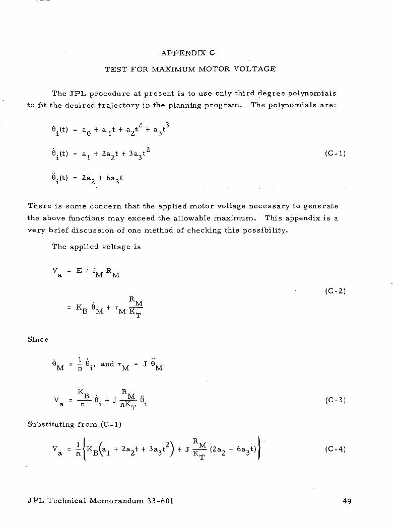
The JPL procedure at present is to use only third degree polynomials

to fit the desired trajectory in the planning program. The polynomials are:

6.(t) = a + 2at + 3at (C- i ;

6 (t) = 2a2 + 6a3t

There is some concern that the applied motor voltage necessary to generate

the above functions may exceed the allowable maximum. This appendix is a

very brief discussion of one method of checking this possibility.

The applied voltage is

V = E + i. , R A / ra M M

R e.. + T. . ^~B M M K^,

(C-2)R,

Since

6.. = - 6., and T., = J 0'M n i M M

v = —2- e. + J-^ e. (c-3)a n i nKT i

Substituting from (C- l )

^ = k[*


Taking the derivative and setting it equal to zero, and solving for t results

in

a2(C-5)

Now, compute V from (C-4) using t from (C-5). If its value is larger thanct

a given maximum, the trajectory is undesirable because the motor torque

will not be as large as required to follow the trajectory in (C-l) . Of course,

the error signals will eventually bring the error to zero, but the resultant

deviation before this may be undesirable. In any respect, depending on the

error signals for large errors defeats the purpose of the computed torque sys-

tem, and the operation is then much like a conventional position servo.

50 JPL, Technical Memorandum 33-601

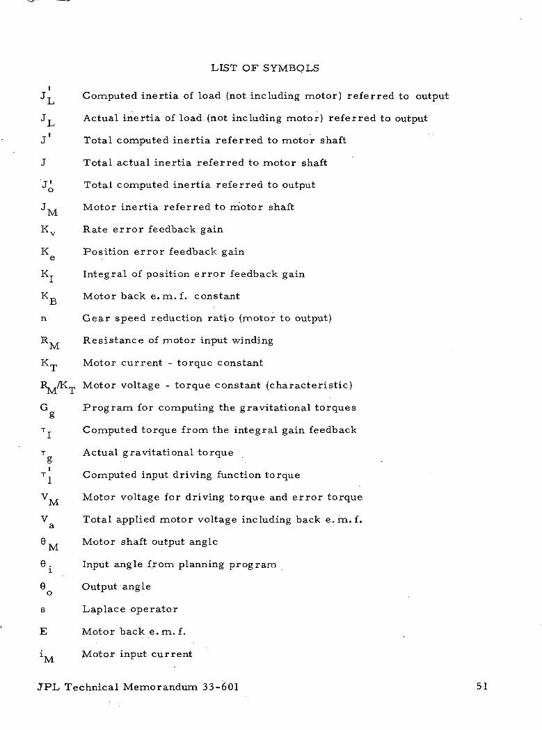
LIST OF SYMBOLS

tJ, Computed inertia of load (not including motor) referred to output

JT Actual inertia of load (not including motor) referred to output

J Total computed inertia referred to motor shaft

J Total actual inertia referred to motor shaft

J' Total computed inertia referred to output

J, , Motor inertia referred to motor shaftM

KV Rate error feedback gain

K Position error feedback gain

KT Integral of position error feedback gain

K Motor back e.m.f. constantr>

n Gear speed reduction ratio (motor to output)

R- , Resistance of motor input winding

K_, Motor current - torque constant

Motor voltage - torque constant (characteristic)

G Program for computing the gravitational torquesO

T Computed torque from the integral gain feedback

T Actual gravitational torqueO

T Computed input driving function torque

"V\, Motor voltage for driving torque and error torque

V Total applied motor voltage including back e.m.f.3-

0.., Motor shaft output angle

6 . Input angle from planning program

6 Output angle

s Laplace operator

E Motor back e.m.f.

L , Motor input currentM ^


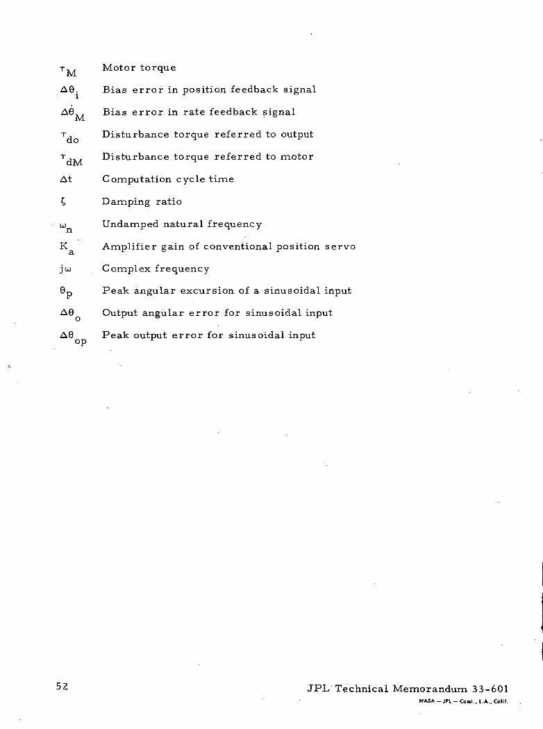
T,., Motor torque

A9. Bias error in position feedback signal

A6 Bias error in rate feedback signal

TJ Disturbance torque referred to output

T Disturbance torque referred to motor

At Computation cycle time

£, Damping ratio

oo Undamped natural frequency

K Amplifier gain of conventional position servocL

jw Complex frequency

0p Peak angular excursion of a sinusoidal input

A6 Output angular error for sinusoidal input

A0 Peak output error for sinusoidal inputop ^ r

52 JPL Technical Memorandum 33-601NASA - JPL - Coml., L.A., Calif.

TECHNICAL REPORT STANDARD TITLE PAGE

1. Report No. 33-601 2. Government Accession No. 3. Recipient's Catalog No.

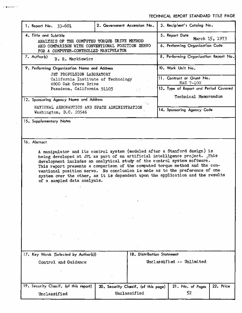
4. Title and SubtitleANALYSIS OF THE COMPUTED TORQUE DRIVE METHODAND COMPARISON WITH CONVENTIONAL POSITION SERVOFOR A COMPUTER-CONTROLLED MANIPULATOR

5. Report DateMarch l£, 1973

6. Performing Organization Code

7. Author (s) B. R. Markiewicz 8. Performing Organization Report No.

9. Performing Organization Name and Address

JET PROPULSION LABORATORYCalifornia Institute of Technology4800 Oak Grove DrivePasadena, California 91103

10. Work Unit No.

11. Contract or Grant No.NAS 7-100

12. Sponsoring Agency Name and Address

NATIONAL AERONAUTICS AND SPACE ADMINISTRATIONWashington, D.C. 20546

13. Type of Report and Period Covered

Technical Memorandum

14. Sponsoring Agency Code

15. Supplementary Notes

16. Abstract

A manipulator and its control system (modeled after a Stanford design) isbeing developed at JPL as part of an artificial intelligence project,development includes an analytical study of the control system software.This report presents a comparison of the computed torque method and the con-ventional position servo. No conclusion is made as to the preference of onesystem over the other, as it is dependent upon the application and the resultsof a sampled data analysis.

17. Key Words (Selected by Author(s))

Control and Guidance

18. Distribution Statement

Unclassified — Unlimited

19. Security Clossif. (of this report)

Unclassified

20. Security Clossif. (of this page)

Unclassified

21. No. of Pages

52

22. Price

HOW TO FILL OUT THE TECHNICAL REPORT STANDARD TITLE PAGE

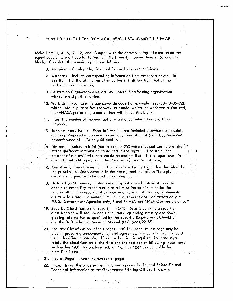
Make items 1, 4, 5, 9, 12, and 13 agree with the corresponding information on thereport cover. Use all capital letters for title (item 4). Leave items 2, 6, and 14-blank. Complete the remaining items as follows:

3. Recipient's Catalog No. Reserved for use by report recipients. .

7. Author(s). Include corresponding information from the report cover. Inaddition, list the affiliation of an author if it differs from that of theperforming organization.

8. Performing Organization Report No. Insert if performing organizationwishes to assign this number.

10. Work Unit No. Use the agency-wide code (for example, 923-50-10-06-72),which uniquely identifies the work unit under which the work was authorized.Non-NASA performing organizations will leave this blank.

11. Insert the number of the contract or grant under which the report wasprepared.

15. Supplementary Notes. Enter information not included elsewhere but useful,such as: Prepared in cooperation with... Translation of (or by)... Presentedat conference of... To be published in...

16.''Abstract. Include a brief (not t'o exceed 200 words) factual summary-of the •• most significant information contained in the report. If possible, the <'abstract of a classified report should be unclassified. If the report contains

' ' ' a significant bibliography or literature survey, mention it here.

17. -Key Words. Insert terms or short phrases selected by the author that identifythe principal subjects covered in the report, and that are(sufficiently .specific and precise to be used for cataloging.

18. Distribution Statement. Enter one of the authorized statements used todenote releasability to the public or a limitation on dissemination forreasons other than security of defense information. Authorized statementsare "Unclassified—Unlimited, " "U.S. Government and Contractors only, ""U. S. Government Agencies only, " and "NASA and NASA Contractors only. "

19. Security Classification (of report). NOTE: Reports carrying a securityclassification will require additional markings giving security and down-grading information as specified by the Security Requirements Checklistand the DoD Industrial Security Manual (DoD 5220. 22-M).

20. Security Classification (of this page). NOTE: Because this page may beused in preparing announcements, bibliographies, and data banks, it shouldbe unclassified if possible. If a classification is required, indicate sepa-rately the classification of the title and the abstract by following these itemswith either "(U)" for unclassified, or "(C)" or "(S)" as applicable for

1 " . : classified items;". ' • ' • ' . • • • . . ' ' • • j

21. No. of Pages. Insert the number of pages.

22. Price. Insert the price set by the Clearinghouse for Federal Scientific andTechnical Information or the Government Printing Office, if known.

Documents

Analysis of the Computed Torque Drive Method and ... AERONAUTICS AND SPACE ADMINISTRATION Technical Memorandum 33-601 Analysis of the Computed Torque Drive Method and Comparison With