Analysis of the dynamic modeling method of articulated ...jestr.org/downloads/Volume10Issue3/fulltext41032017.pdf · Analysis of the Dynamic Modeling Method of Articulated Vehicles

Journal of Engineering Science and Technology Review 10 (3) (2017) 18- 27

Research Article

Analysis of the Dynamic Modeling Method of Articulated Vehicles

Qingyong Meng 1, 3*, Lulu Gao 1, Heping Xie 3 and Fengqian Dou 2

1 School of Mechanical Engineering of USTB, Beijing 100083, China

2 School of Mechanical and Mechatronics Engineering of UW, Canada 3 XCMG Mining Machinery Co., Ltd., Xuzhou, Jiangsu 221000, China

Received 12 January 2017; Accepted 21 June 2017

___________________________________________________________________________________________ Abstract

Most of the existing research related to the handling stability of articulated vehicles takes the front wheel angle as input and neglects the influence of the steering system and regards these vehicles as moving in planes that parallel the ground plane. The established dynamic model cannot meet the requirements of stability control under unmanned and high-speed working conditions. This research proposed a fusion modeling method based on the kinematics and dynamics of vehicles to improve the precision of a driving dynamic model. The proposed method initially took the steering wheel angle as input to establish the kinematic model for the corresponding relation of the hydraulic system flow and pressure, the articulated angle of front and rear frames, and the output force of left and right steering hydraulic cylinders. A dynamic model considering the axle load transfer and interactions between the front frame and the rear body in a three-dimensional coordinate system was then established. A driving dynamic model of an entire vehicle was also constructed by coupling the kinematic and dynamic models. Finally, real vehicle test data of a 60-ton articulated vehicle were used to verify the proposed Automatic Dynamic Analysis of Mechanical Systems (ADAMS) driving model in this study. Results confirm that the error about the steady-state yaw rate in the simulation and real vehicle tests did not exceed 0.01 rad/s. Therefore, the established driving dynamic model can describe the dynamic response accurately. This study concludes that the proposed fusion modeling method based on the combination of kinematics and dynamics can effectively improve the accuracy of the articulated vehicle model and further provide a technical reference for the study on a driving stability control strategy.

Keywords: Combination modeling, Control strategy, Articulated vehicle __________________________________________________________________________________________ 1. Introduction The improvement of transportation efficiency and the reduction of production costs for constructing water conservancy work and mining transportation by increasing the speed of transportation vehicles and adopting unmanned driving technologies are currently imperative. Articulated steering vehicles (ASVs) adopt fully hydraulic, full-wheel driving and articulated steering with excellent traffic capability and flexibility, which have been widely used in constructing water conservancy work and mining transportation. Unlike traditional transportation vehicles, articulated vehicles consist of front and rear parts, which are connected by the kingpin mounted perpendicularly on the ground and the articulated joint paralleling the vehicle direction. The articulated vehicles cannot go straight because no dip angle of the connecting kingpin exists, which may also result in the snaking phenomenon at high speed. Relative rotation between front and rear frames will cause significant tipping during vehicle steering. For the articulated vehicles currently used in constructing water conservancy work and mine transportation, the highest speed is, thus, limited for safety. For example, although the design

speed of Doosan DA40 can reach 55 /km h , the actual operation speed at the Ken Swat Hydro-junction in Xinjiang is below 25 /km h , which has severely affected the production efficiency. Vehicle driving and steering stability can be effectively guaranteed and vehicle travel speed can be increased by adopting active safety technology for articulated vehicles. Active safety technology adopts multi-sensor fusion technology, which is used to monitor the vehicle state. Stability model and indicator are then adopted to investigate the vehicle dynamic stability according to the vehicle state, and the vehicle dynamic stability is finally improved through anti-tipping methods [1, 2].

Considerable research on multi-sensor fusion and observer technology has been conducted [3-5]. However, neither the key dynamic parameters, such as yaw velocity, can be estimated nor the stability can be controlled effectively because of the oversimplified dynamic model. The effectiveness of active safety technology is determined by the accuracy of the dynamic model of ASVs. The dynamic model of articulated vehicles is important in the vehicle design stage and a key technology for the active safety control design. Therefore, a three-dimensional modeling method should be adopted to improve the accuracy of the estimated yaw rate value for articulated vehicles. Such method can provide reliable support for the active safety technology and, thus, increase the travel speed under the complicated road conditions during the construction of water conservancy work.

JOURNAL OF Engineering Science and Technology Review

www.jestr.org

Jestr

______________ *E-mail address: [email protected]

ISSN: 1791-2377 © 2017 Eastern Macedonia and Thrace Institute of Technology. All rights reserved. doi:10.25103/jestr.103.04

Qingyong Meng, Lulu Gao, Heping Xie and Fengqian Dou/Journal of Engineering Science and Technology Review 10 (3) (2017) 18-27

19

2. State of the art

The electronic stability program (ESP) can improve vehicle maneuver capability on dangerous working conditions through the motion control of the vehicle in lateral, longitudinal, and vertical directions [6, 7]. The system mainly depends on three parts, namely, the observer, the control strategy, and the executive control. The longitudinal speed, horizontal speed, yaw velocity, tire-road friction coefficient, and other dynamic parameters of the observer model are crucial for the ESP to obtain sideslip angle accurately [8-10]. Polotski and Hemami proposed a theoretical model for mine shearers and conducted considerable experimental research on the dynamics of ASVs and tracking control problems under a given path. A linear feedback control algorithm for path tracking was finally presented. However, dynamic problems were not considered because the hypothetical vehicle speed in the model was very slow and would not produce high acceleration; hence, the model could be regarded as a kinematic model [11]. Yavin proposed a four-degree-of-freedom (4DOF) dynamic model for wheel loader, transport vehicle, and dump truck driving on smooth ground based on the Lagrangian equation, which could be used to simulate the ground force and movement acted on the vehicle and analyze the influence of masses and rotational inertia of vehicles [12]. The aforementioned parameters are mainly obtained from the vehicle kinematics or nonlinear dynamics. Compared with kinematics, dynamics has more advantages in the aspects of robustness and stability and more precise in obtaining parameters [13-15]. For an articulated vehicle, most of the studies on the two mentioned aspects are simplified due to the complexity of the hydraulic system and the articulated structure resulting from adopting full hydraulic power steering [16-17]. The hydraulic system is generally equivalent to a linear spring and a constant coefficient damping system. The hydraulic system of the articulated vehicle is simulated by fitting parameters, and the dynamic characteristics are described by an equation of plane motion to avoid the complexity of the articulated frame modeling and dynamic equation. This modeling method can greatly simplify the entire vehicle model and analyze stability-influencing factors quantitatively to some extent. However, the mechanical characteristics of the hinge points of front and rear frames and the hydraulic steering system characteristic in the entire vehicle model are neglected, which can cause considerable errors between simulation study and actual situation and impede the accurate analysis of the stability of articulated mining trucks.

The dynamic mathematical modeling of articulated vehicles are accordingly evaluated based on the three-dimensional coordinate system and the dynamic characteristics of the steering system to provide an accurate control model for the stability control strategy.

This study is organized as follows. Section 1 introduces the modeling of the hydraulic steering system for articulated vehicles. The steering kinematics of articulated vehicles is analyzed to establish the change relation between the displacement velocity of the steering hydraulic cylinder and the articulated angle and, thus, the hydraulic steering system model. Section 2 discusses about the vehicle dynamic model coupled with hydraulic steering. Section 3 proposes the fusion modeling method and deals with the driving dynamic model by coupling the kinematics and dynamics of vehicle. Section 4 discusses the validity of the proposed driving

dynamic model through a real vehicle test. Section 5 presents the conclusions and expectations. 3. Methodology 3.1 Steering kinematic model

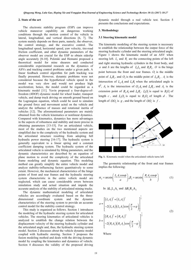
The kinematic modeling of the steering system is necessary to establish the relationship between the output force of the steering hydraulic cylinder and the steering articulated angle. Figure 1 shows the kinematic model of an ASV when steering left. 1L and 1R are the connecting points of the left and right steering hydraulic cylinders in the front body, and a and b are the lengths of 1 2LL and 1 2R R . O is the hinge point between the front and rear frames. 1O is the middle point of 1 1LR , and 2O is the middle point of 2 2L R . 1A is the intersection of 2 1L A and 1 1LR when the articulated angle is 00, 3A is the intersection of 2 3O A and 1 1LR , and 2A is the extension point of 2 3R A and 1 1LR . 1 1LO is equal to 1 1RO of length c , and 2 2L O is equal to 2 2R O of length d . The length of 2OO is g , and the length of 1OO is f .

Fig. 1. Kinematic model when the articulated vehicle turns left

The geometric relationship of the front and rear frames implies the following:

α 2 = arcsin

L1A1 cosϕa

⎛⎝⎜

⎞⎠⎟

,β2 = arcsinR1A2 cosϕ

b⎛⎝⎜

⎞⎠⎟

(1)

In 1 2 1 L L AΔ and 1 2 2R R AΔ

( ) ( )

( )( )

( ) ( )

( )( )

12 2 2

1 1 2 1

1 1 2 1

12 2 2

1 2 2 2

1 2 2 2

2 cos2

2 cos2

L A L Aa

L A L A

R A R Ab

R A R A

πϕ

πϕ

⎡ ⎤+⎢ ⎥

= ⎢ ⎥⎛ ⎞− +⎜ ⎟⎢ ⎥⎝ ⎠⎣ ⎦

⎡ ⎤+⎢ ⎥

= ⎢ ⎥⎛ ⎞− −⎜ ⎟⎢ ⎥⎝ ⎠⎣ ⎦

(2)

Where


20

1 1

2 1

1 2

2 2

tancos

tancos

tancos

tancos

dL A c f

fL A g d

cR A c f

fR A g d

ϕφ

ϕφ

ϕφ

ϕφ

= − −

= + +

= − +

= + −

(3)

Figure 2 shows the steering mechanism of the articulated

dump truck during straight driving, where 1OP is the base height of 2 1L OLΔ , which is referred to as 1h ; 2OP is the base height of 2 1R ORΔ , which is referred to as 2h ; those heights are the arm lengths of the left and right steering cylinders to the hinge point, respectively; and 2OL is equal to 1OR and referred to as r .

Fig. 2. Steering mechanism of the articulated vehicle

When the vehicle turns left,

2 1

2 1

L OLR OR

δ δ

δ δ

∠ = − Δ

∠ = + Δ (4)

In ΔL2OL1 and ΔR2OR1, according to the triangle area

formula, the areas are as follows:

1

2

1 1 sin( )2 21 1 sin( )2 2

h a Rr

h b Rr

δ δ

δ δ

× × = − Δ

× × = + Δ

(5)

Accordingly,

1

2

sin( )

sin( )

Rrha

Rrhb

δ δ

δ δ

− Δ=

+ Δ=

(6)

During the steering process of the articulated truck, the

left and right steering cylinder movements take the hinge point as circle center to perform circular motion, the angular velocity is the change rate of the articulated angle, and the displacement velocities of the left and right steering hydraulic cylinder piston rods relative to piston cylinders 01u and 02u are as follows:

.

01 1.

02 2

( )

( )

u h

u h

δ δ

δ δ

= × −Δ

= × +Δ (7)

3.2 Steering dynamic model The articulated vehicle adopts full hydraulic steering, steering wheel angle change control, and the opening change of the steering gear settable orifice. The hydraulic oil enters the left and right steering cylinders through the main valve and output steering torque. The relation equation for input/output flow, steering cylinder output force, and the articulated angle of the front and rear frames is established according to the relationship between the system flow and the displacement of the steering cylinder piston.

The steering wheel angle input is ε. Under the steering wheel control, the system output is Q , where

= dQ qdtε (8)

Figure 3 shows the left and right steering cylinder system

of the articulated vehicle. 1LP and 1RP denote the pressure of the left and right steering cylinder rod ports, respectively. 1LQ and 1RQ denote the input and output flows of the left and right steering cylinder rod ports, respectively. 2LP and 2RP denote the input and output flows of the left and right steering cylinder head ports, respectively. 2LQ and 2RQ denote the input and output flows of the left and right steering cylinder head ports, respectively. LF and RF denote the steering forces provided by the left

and right steering cylinders, respectively.

. Fig. 3. Input/output relationship of steering cylinders for the articulated vehicle

The flows of the left and right steering cylinder fuel inlet

chambers 1LQ and 2RQ are expressed as follows:

1 11

2 22

+

+

L L LL L r

R R RR L p

dX V dPQ Q Adt B dtdX V dPQ Q Adt B dt

= +

= +

(9)

where LQ is the leakage volume of hydraulic oil. pA is

the cross-sectional area of the steering cylinder head port, and rA is the cross-sectional area of the steering cylinder rod


21

port. LX is the piston displacement of the left steering cylinder, and RX is the piston displacement of the right steering cylinder. B is the effective bulk elastic modulus, including hydraulic oil, pipeline, and the mechanical compliance of the steering cylinder body. 1LV is the oil volume of the left steering cylinder head port, and 2RV is the oil volume of the right steering cylinder rod port. The first item in the equation is the oil leakage amount of the hydraulic cylinder, which can be obtained by 1 2( )L ipQ C P P= − , and ipC is the leakage coefficient. The second item is the volume variation of the hydraulic cylinder. The third item is the required flow for oil compressibility,

where LdXdt

and RdXdt

are the displacement speeds of the left

and right steering cylinders, respectively; they are substituted with kinematic analysis expression (7), and the following expression is then obtained:

.

1

.

2

( )

( )

L

R

dX hdtdX hdt

δ δ

δ δ

= × − Δ

= × + Δ

(10)

The total flow input and output of the hydraulic cylinder

are 1Q and 2Q , respectively.

.1 1

1 1 2 1 2

.2 2

2 1 2 1 2

( ) 2 ( )

( ) 2 ( )

r p ip

p r ip

V dPQ A h A h C P PB dtV dPQ A h A h C P PB dt

δ

δ

= + × + × − +

= + × + × − −

(11)

Equations (8) and (11) are combined, and the pressure of

the hydraulic cylinder oil inlet delivery cavities 1P and 2P can be obtained.

Given the speed of the steering wheel,

11 2

1

1 2

2

= ( ( )

2 ( ))

0

r p

ip

dP B d dq A h A hdt V dt dt

C P PdPdt

ε δ⎧ − +⎪⎪⎪

− × −⎨⎪⎪ =⎪⎩

(12)

When the speed of the steering wheel angle 0ddtε= ,

11 2 1 2

1

21 2 1 2

1

= ( ) 2 ( )

( ) 2 ( )

r p ip

p r ip

dP B dA h A h C P Pdt V dtdP B dA h A h C P Pdt V dt

δ

δ

⎧ − + − × −⎪⎪⎨⎪ = − + − × −⎪⎩

(13)

The steering force of the left and right steering

cylinders LF and RF can be obtained according to the pressure in and out of oil cavities 1P and 2P as follows:

1 2

2 1

L p r

R p r

F PA P AF P A PA= −

= − (14)

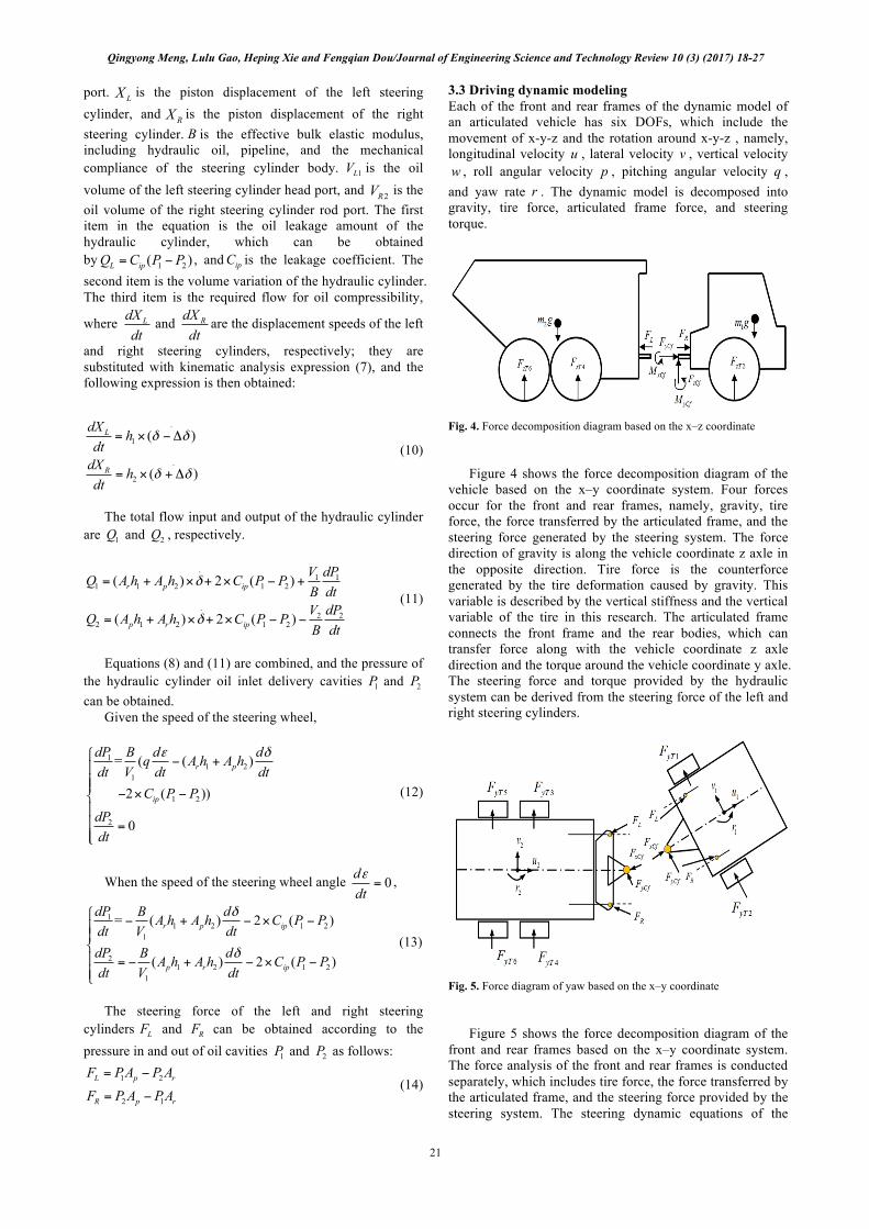
3.3 Driving dynamic modeling Each of the front and rear frames of the dynamic model of an articulated vehicle has six DOFs, which include the movement of x-y-z and the rotation around x-y-z , namely, longitudinal velocity u , lateral velocity v , vertical velocity w , roll angular velocity p , pitching angular velocity q , and yaw rate r . The dynamic model is decomposed into gravity, tire force, articulated frame force, and steering torque.

Fig. 4. Force decomposition diagram based on the x–z coordinate

Figure 4 shows the force decomposition diagram of the vehicle based on the x–y coordinate system. Four forces occur for the front and rear frames, namely, gravity, tire force, the force transferred by the articulated frame, and the steering force generated by the steering system. The force direction of gravity is along the vehicle coordinate z axle in the opposite direction. Tire force is the counterforce generated by the tire deformation caused by gravity. This variable is described by the vertical stiffness and the vertical variable of the tire in this research. The articulated frame connects the front frame and the rear bodies, which can transfer force along with the vehicle coordinate z axle direction and the torque around the vehicle coordinate y axle. The steering force and torque provided by the hydraulic system can be derived from the steering force of the left and right steering cylinders.

Fig. 5. Force diagram of yaw based on the x–y coordinate

Figure 5 shows the force decomposition diagram of the front and rear frames based on the x–y coordinate system. The force analysis of the front and rear frames is conducted separately, which includes tire force, the force transferred by the articulated frame, and the steering force provided by the steering system. The steering dynamic equations of the


22

articulated vehicles established based on a three-dimensional coordinate system are as follows:

mi !ui − mi (rivi − qiwi ) = FxTi + FxHi + FxCi + FxGi

mi !vi − mi ( piwi − riui ) = FyTi + FyHi + FyCi + FyGi

mi !wi − mi (qiui − pivi ) = FzTi + FzTi + FzCi + FzGi

Ixxi !pi − (I yyi − Izzi )qiri = MxTi + MxHi + MxCi

I yyi !qi − (Izzi − Ixxi ) piri = M yTi + M yHi + M yCi

Izzi !ri − (Ixxi − I yyi )qi pi = MzTi + MzHi + MzCi

(14)

For the left side of the equations, 1,2i = stands for the

front and rear frames; im is the frame mass; xxiI , yyiI , and

zziI are the moment of inertia around the axle in the frame centroid; , ,k x y z= stands for the action direction of force in a relative coordinate; kTiF is the force of the front and rear frames applied by the tire; and kTiM is the corresponding torque generated by the tire. kHiF is the force of the front and rear frames in the k direction applied by a hydraulic system, and kHiM is the corresponding torque generated by the hydraulic system. kCiF is the force of the front and rear frames in the k direction applied by the articulated body, and kCiM is the corresponding torque transferred by the articulated body. kGiF is the force of the front and rear frames in the k direction applied by gravity, and kGiM is the corresponding torque generated by gravity. 3.4 Coupling equation of speed The acceleration equation in three directions under the vehicle steering working condition is established based on the x–y–z vehicle coordinate system as follows:

.

.

.

x

y

z

a u vr wq

a v wp ur

a w uq vp

= − +

= − +

= − +

(16)

where xa , ya , and za are the accelerations in the three

directions of the x–y–z coordinate system, respectively. u , v , and w are the lateral velocities in three directions based on the x-y-z coordinate system. r , p , and q are the angular velocities in the three directions based on the x-y-z coordinate system.

3.5 Torque equation in hinge points Figure 5 depicts that the front and rear frames transfer torques from the three directions of x-y-z and the three directions around x-y-z . The rolling moment around x axle and the pitch moment around y applied in the hinge point are as follows:

2( )xCf yCf Cf

yCf C f r xCf Cf zCf f

M F ZM K F Z F Lθ θ θ

=

= − + + (17)

3.6 Dynamic model of tire Vertical tire force is expressed by linear vertical stiffness and deformation as follows:

;( 1,2,3,4,5,6)zTl zT lF K l= − Δ = (18)

where lΔ is the vertical dynamic deflection, 0l l lz zΔ = − .

lz is related to frame roll and pitch motion, and 0lz is the vertical static deflection. The lateral force of the tire is expressed by cornering stiffness and sideslip angle as the following: yTi ai iF K a= (19)

where aiK is the cornering stiffness of the tire. ia is the

sideslip angle corresponding to the tire. The cornering stiffness of tire aiK varied from vertical loads and expressed by the following:

2 2

2

60 1.7 12.7( ) ( 0.088)

60 0.095 0.49 ( 0.088)

t ti i i

ai

t ti i

l l lpD D D

Kl lpD D

ω

ω

⎧ ⎡ ⎤Δ Δ Δ− ≤⎪ ⎢ ⎥

⎪ ⎣ ⎦= ⎨

⎡ ⎤Δ Δ⎪ − >⎢ ⎥⎪⎣ ⎦⎩

(20)

where tp is the tire inflation pressure, tω is the tire

nominal width, and lΔ is the tire radial compression. Sideslip angle ia can be derived from the following

formulas:

1 1 11

1 1

1 1 12

1 1

2 3 23

2 2

2 3 24

2 2

2 1 25

2 2

2 1 26

2 2

f

f

r

r

r

r

v L ra

u Trv L r

au Tv L rau Trv L rau Trv L rau Trv L rau Tr

ω

+=

−

−=

+

+=

−

+=

+

−=

−

−=

+

(21)

The output force and torque acting on the front frame by

tires are as follows:

1 2

1 2

1 2

1 1 2 1

1 1 2 1

yTf yT yT

zTf zT zT

xTf zT zT

yTf zT f zT f

zTf yT f yT f

F F FF F FM F T F TM F L F LM F L F L

= +

= +

= ⋅ − ⋅

= ⋅ + ⋅

= − ⋅ − ⋅

(22)

The force and torque acting on the rear frame by tires are

as follows:


23

3 4 5 6

3 4 5 6

3 4 5 6

3 3 4 3 5 1 6 1

3 3 4 3 5 1 6 1

yTr yT yT yT yT

zTf zT zT zT zT

xTr zT zT zT zT

yTr zT r zT r zT r zT r

zTr yT r yT r yT r yT r

F F F F FF F F F FM F T F T F T F TM F L F L F L F LM F L F L F L F L

= + + +

= + + +

= ⋅ − ⋅ + ⋅ − ⋅

= − ⋅ − ⋅ + ⋅ − ⋅

= ⋅ + ⋅ − ⋅ − ⋅

(23)

3.7 Output force and torque equation of the steering system The force and torque equations acting on the front frame by the steering system can be confirmed while turning according to Figure 5, i.e.,

1 1

1 1

1 1

1 1

cos + cos

sin sin

( cos + cos )

( sin sin )

xHf L R

yHf L R

xHf yHf Hf

zHf L R

L R

F F FF F FM F ZM F F a

F F b

α β

α β

α β

α β

=

= −

= ⋅

= − ⋅

+ − − ⋅

(24)

The force and torque equations acting on the rear frame

by the steering system are the following:

2 2

2 2

2 2

2 2

cos sinsin sin

( cos sin )( sin sin )

xHr L R

yHr L R

xHr yHr Hr

zHr L R

L R

F F FF F FM F ZM F F c

F F d

α β

α β

α β

α β

= − −

= − +

= ⋅

= − ⋅

+ − + ⋅

(25)

3.8 Additional equations

The force and torque equations acting on the front frame

by the steering system can be confirmed while turning according to Figure 5, i.e.,

1 1

1 1

1 1

1 1

cos + cos

sin sin

( cos + cos )

( sin sin )

xHf L R

yHf L R

xHf yHf Hf

zHf L R

L R

F F FF F FM F ZM F F a

F F b

α β

α β

α β

α β

=

= −

= ⋅

= − ⋅

+ − − ⋅

(26)

The force and torque equations acting on the rear frame

by the steering system are the following:

2 2

2 2

2 2

2 2

cos sinsin sin

( cos sin )( sin sin )

xHr L R

yHr L R

xHr yHr Hr

zHr L R

L R

F F FF F FM F ZM F F c

F F d

α β

α β

α β

α β

= − −

= − +

= ⋅

= − ⋅

+ − + ⋅

(27)

4. Result Analysis and discussion

The mathematical model is verified through the real vehicle test data and Automatic Dynamic Analysis of Mechanical Systems (ADAMS) simulation data to ensure the accuracy of the mathematical model. Tab. 1. presents the basic parameters of the vehicle, including the front and rear frame

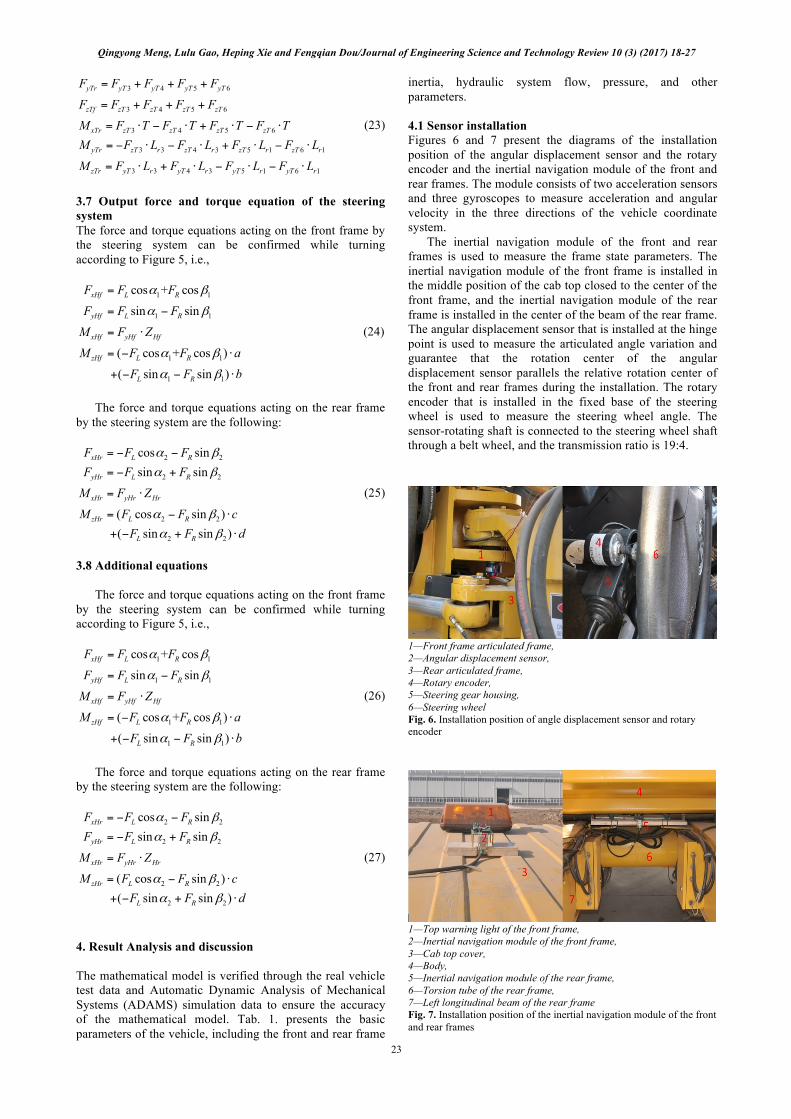
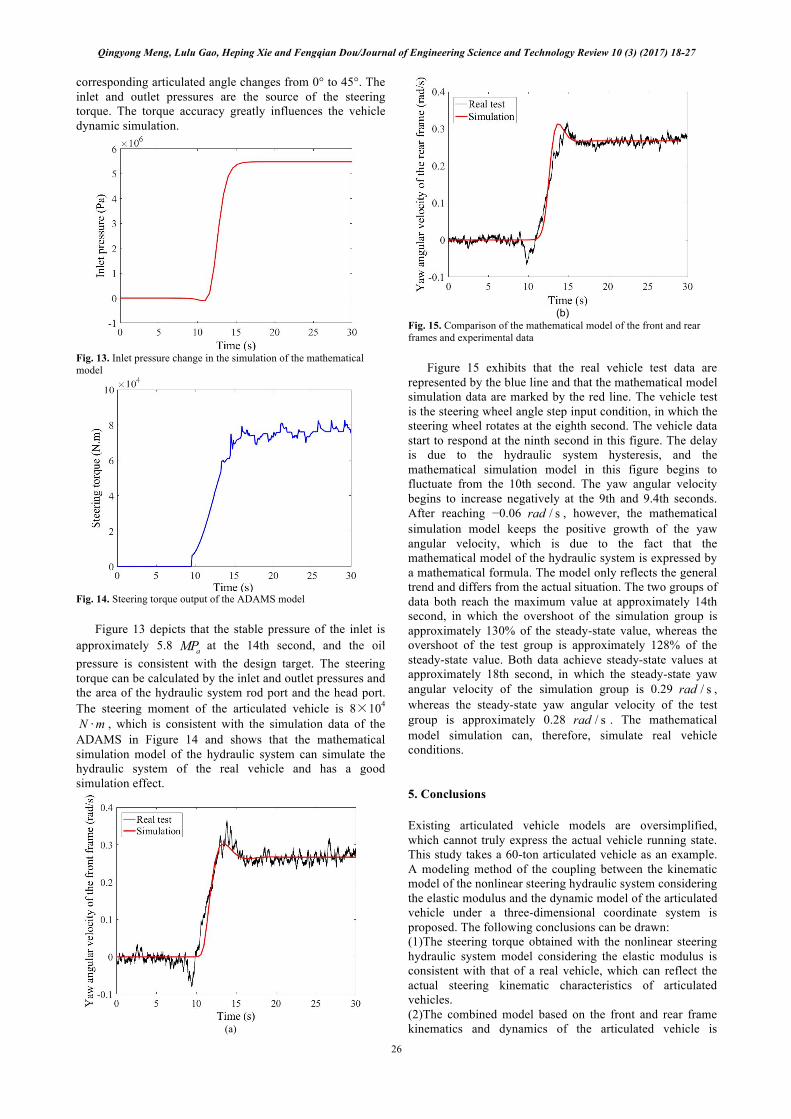
inertia, hydraulic system flow, pressure, and other parameters. 4.1 Sensor installation Figures 6 and 7 present the diagrams of the installation position of the angular displacement sensor and the rotary encoder and the inertial navigation module of the front and rear frames. The module consists of two acceleration sensors and three gyroscopes to measure acceleration and angular velocity in the three directions of the vehicle coordinate system. The inertial navigation module of the front and rear frames is used to measure the frame state parameters. The inertial navigation module of the front frame is installed in the middle position of the cab top closed to the center of the front frame, and the inertial navigation module of the rear frame is installed in the center of the beam of the rear frame. The angular displacement sensor that is installed at the hinge point is used to measure the articulated angle variation and guarantee that the rotation center of the angular displacement sensor parallels the relative rotation center of the front and rear frames during the installation. The rotary encoder that is installed in the fixed base of the steering wheel is used to measure the steering wheel angle. The sensor-rotating shaft is connected to the steering wheel shaft through a belt wheel, and the transmission ratio is 19:4.

1—Front frame articulated frame, 2—Angular displacement sensor, 3—Rear articulated frame, 4—Rotary encoder, 5—Steering gear housing, 6—Steering wheel Fig. 6. Installation position of angle displacement sensor and rotary encoder

1—Top warning light of the front frame, 2—Inertial navigation module of the front frame, 3—Cab top cover, 4—Body, 5—Inertial navigation module of the rear frame, 6—Torsion tube of the rear frame, 7—Left longitudinal beam of the rear frame Fig. 7. Installation position of the inertial navigation module of the front and rear frames


24

Table 1. Parameters of the 60-ton electric articulated vehicle driven by a wheel motor

Vehicle parameters (front frame) Parameter Value Parameter Value Parameter Value u 10 /km h 1fL 0.5 m a 0.8 m

1m 18316.58 kg 2fL 2.1 m b 0.3 m

1xxI 32013.97 2kg m⋅ CfZ 0.02 m f 1.8 m

1yyI 31296.98 2kg m⋅ TfZ 1.29 m T 1.6 m

1zzI 47686.92 2kg m⋅ HfZ 0.02 m Vehicle parameters (rear frame, empty load)

2m 21050.17 kg 1rL 1.35 m c 0.64 m

2xxI 42419.84 2kg m⋅ 2rL 3.15 m d 0.7 m

2yyI 76641.08 2kg m⋅ 3rL 0.65 m g 0.245 m

2zzI 94476.50 2kg m⋅ CrZ 0.18 m HrZ 0.18 m

TrZ 1.49 m Vehicle parameters (rear frame, full load)

2m 87801.07 kg 1rL 1.45 m CrZ 0.38 m

2xxI 72420.75 2kg m⋅ 2rL 3.05 m TrZ 1.79 m

2yyI 96641.1 2kg m⋅ 3rL 0.55 m HrZ 0.38 m

2zzI 151645 2kg m⋅ d 2.895 m Hydraulic system

1OLV 6.4×10-3 3m pA 12.3×10-3 2m R 1.97 m

2OLV 3.6×10-3 3m rA 8.4×10-3 2m r 0.685 m

1ORV 6.4×10-3 3m B 3×109 aP

2ORV 3.6×10-3 3m 2P 2 aMP

Comparative analysis of the real vehicle test, the ADAMS model, and the simulation mathematical model 4.2 Working condition setting and ADAMS model setting The test adopts transient steering working condition, namely, steering wheel angle step input, in which the steering wheel angle is measured by a rotary encoder, and the change trend of angle is shown in Figure 9.

Fig. 8. Steering wheel angle data of the real vehicle test

Figure 8 shows that the vehicle drives along a straight line at 10 /km h . The steering wheel angle is 0 rad at the first 8 s, and then the steering wheel turns left until the 14th second. The total turn steering angle is 12 rad , and the average angular velocity is 2 / srad .

The ADAMS simulation model simulates the operating condition of the real vehicle, keeps the speed at 10 /km h , inputs the steering cylinder force, and makes the steering condition consistent with the real vehicle test. Figure 9 depicts the variation in the articulated angle. A linear relation exists between the articulated and steering wheel angles.

Fig. 9. Articulated angle data of the ADAMS simulation model


25

4.3 Comparison of responses

(a)

(b)

Fig. 10. Comparison of data between the real vehicle test and the ADAMS simulation

In Figures 10, the real vehicle test data are shown in black, whereas the ADAMS simulation data are shown in blue. The vehicle test is the steering wheel angle step input condition, and the steering wheel rotates at the eight second. The vehicle data start to respond at the ninth second in this figure, and the delay is due to the hydraulic system hysteresis. The ADAMS simulation data in this figure begin to fluctuate from the ninth second because the modeling of the hydraulic system is simplified modeling, which uses the driving force instead of the hydraulic pressure.

The yaw angular velocity begins to increase negatively at the 9th and 9.4th seconds. After reaching −0.06 / srad , the yaw angular velocity starts to return to zero and increases with the steering wheel angle. The situation is that the steering pressure is insufficient for the vehicle steering when the hydraulic steering system starts and causes a slight swing around. With the rapid rise in the oil pressure, the vehicle begins to steer smoothly. The two groups of data reach the maximum value in approximately 14 s , in which the overshoot of the simulation group is approximately 135% of the steady-state value, and the overshoot of the test group is approximately 128% of the steady-state value. Both data achieve the steady-state values at approximately the 18th seconds, in which the steady-state yaw angular velocity of the simulation group is 0.29 / srad , whereas the steady-state yaw angular velocity of the test group is approximately 0.28 / srad . The ADAMS simulation model can simulate

real vehicle conditions and can be used for the following validation of the mathematical model simulation of the hydraulic system.

Fig. 11. Steering wheel angle input of the mathematical simulation model Figure 11 depicts the steering wheel angle input of the simulation model, which uses the steering wheel angle input simulated by function as follows:

1 ( 8) 1

11 A t B

Cye × − +

=+

(26)

The simulation condition is that the steering wheel angle is 0 rad to 12 rad from 8 s to 14 s , and the corresponding articulated angle changes from 0° to 45°. The steering rod displacement is achieved by the steering wheel to control the hydraulic system and is the steering force acting on the steering cylinder by oil source, and the front and rear frames of the vehicle rotate relatively. Figure 13 illustrates the verification of the simulation mathematical model of the left and right steering rod displacements.

Fig. 12. Simulation mathematical model of the left and right steering rod displacements

Figure 12 depicts that when the steering wheel angle

reaches the limit, the left steering rod retracts for 1.45 m and that the right steering rod stretches for 2.49 m , Thereby completing the steering process. In the AutoCAD drawing of the real vehicle, the lengths of the left and right steering rods are measured when the articulated angle reaches the limit state, and the results are completely the same.

The simulation condition is that the steering wheel angle is 0 rad to 12 rad from 8 s to 14 s , and the


26

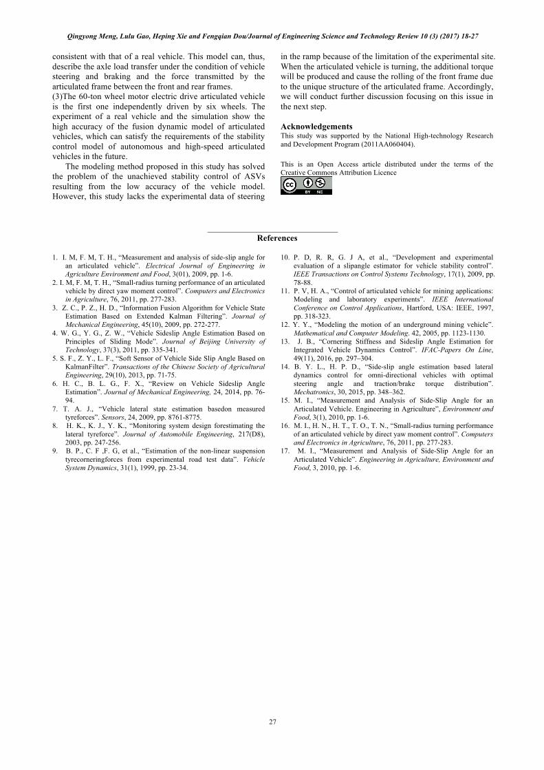
corresponding articulated angle changes from 0° to 45°. The inlet and outlet pressures are the source of the steering torque. The torque accuracy greatly influences the vehicle dynamic simulation.

Fig. 13. Inlet pressure change in the simulation of the mathematical model

Fig. 14. Steering torque output of the ADAMS model

Figure 13 depicts that the stable pressure of the inlet is approximately 5.8 aMP at the 14th second, and the oil pressure is consistent with the design target. The steering torque can be calculated by the inlet and outlet pressures and the area of the hydraulic system rod port and the head port. The steering moment of the articulated vehicle is 8×104 N m⋅ , which is consistent with the simulation data of the ADAMS in Figure 14 and shows that the mathematical simulation model of the hydraulic system can simulate the hydraulic system of the real vehicle and has a good simulation effect.

(a)

(b)

Fig. 15. Comparison of the mathematical model of the front and rear frames and experimental data

Figure 15 exhibits that the real vehicle test data are represented by the blue line and that the mathematical model simulation data are marked by the red line. The vehicle test is the steering wheel angle step input condition, in which the steering wheel rotates at the eighth second. The vehicle data start to respond at the ninth second in this figure. The delay is due to the hydraulic system hysteresis, and the mathematical simulation model in this figure begins to fluctuate from the 10th second. The yaw angular velocity begins to increase negatively at the 9th and 9.4th seconds. After reaching −0.06 / srad , however, the mathematical simulation model keeps the positive growth of the yaw angular velocity, which is due to the fact that the mathematical model of the hydraulic system is expressed by a mathematical formula. The model only reflects the general trend and differs from the actual situation. The two groups of data both reach the maximum value at approximately 14th second, in which the overshoot of the simulation group is approximately 130% of the steady-state value, whereas the overshoot of the test group is approximately 128% of the steady-state value. Both data achieve steady-state values at approximately 18th second, in which the steady-state yaw angular velocity of the simulation group is 0.29 / srad , whereas the steady-state yaw angular velocity of the test group is approximately 0.28 / srad . The mathematical model simulation can, therefore, simulate real vehicle conditions. 5. Conclusions Existing articulated vehicle models are oversimplified, which cannot truly express the actual vehicle running state. This study takes a 60-ton articulated vehicle as an example. A modeling method of the coupling between the kinematic model of the nonlinear steering hydraulic system considering the elastic modulus and the dynamic model of the articulated vehicle under a three-dimensional coordinate system is proposed. The following conclusions can be drawn: (1)The steering torque obtained with the nonlinear steering hydraulic system model considering the elastic modulus is consistent with that of a real vehicle, which can reflect the actual steering kinematic characteristics of articulated vehicles. (2)The combined model based on the front and rear frame kinematics and dynamics of the articulated vehicle is


27

consistent with that of a real vehicle. This model can, thus, describe the axle load transfer under the condition of vehicle steering and braking and the force transmitted by the articulated frame between the front and rear frames. (3)The 60-ton wheel motor electric drive articulated vehicle is the first one independently driven by six wheels. The experiment of a real vehicle and the simulation show the high accuracy of the fusion dynamic model of articulated vehicles, which can satisfy the requirements of the stability control model of autonomous and high-speed articulated vehicles in the future.

The modeling method proposed in this study has solved the problem of the unachieved stability control of ASVs resulting from the low accuracy of the vehicle model. However, this study lacks the experimental data of steering

in the ramp because of the limitation of the experimental site. When the articulated vehicle is turning, the additional torque will be produced and cause the rolling of the front frame due to the unique structure of the articulated frame. Accordingly, we will conduct further discussion focusing on this issue in the next step. Acknowledgements This study was supported by the National High-technology Research and Development Program (2011AA060404). This is an Open Access article distributed under the terms of the Creative Commons Attribution Licence

______________________________

References 1. I. M, F. M, T. H., “Measurement and analysis of side-slip angle for

an articulated vehicle”. Electrical Journal of Engineering in Agriculture Environment and Food, 3(01), 2009, pp. 1-6.

2. I. M, F. M, T. H., “Small-radius turning performance of an articulated vehicle by direct yaw moment control”. Computers and Electronics in Agriculture, 76, 2011, pp. 277-283.

3. Z. C., P. Z., H. D., “Information Fusion Algorithm for Vehicle State Estimation Based on Extended Kalman Filtering”. Journal of Mechanical Engineering, 45(10), 2009, pp. 272-277.

4. W. G., Y. G., Z. W., “Vehicle Sideslip Angle Estimation Based on Principles of Sliding Mode”. Journal of Beijing University of Technology, 37(3), 2011, pp. 335-341.

5. S. F., Z. Y., L. F., “Soft Sensor of Vehicle Side Slip Angle Based on KalmanFilter”. Transactions of the Chinese Society of Agricultural Engineering, 29(10), 2013, pp. 71-75.

6. H. C., B. L. G., F. X., “Review on Vehicle Sideslip Angle Estimation”. Journal of Mechanical Engineering, 24, 2014, pp. 76-94.

7. T. A. J., “Vehicle lateral state estimation basedon measured tyreforces”. Sensors, 24, 2009, pp. 8761-8775.

8. H. K., K. J., Y. K., “Monitoring system design forestimating the lateral tyreforce”. Journal of Automobile Engineering, 217(D8), 2003, pp. 247-256.

9. B. P., C. F ,F. G, et al., “Estimation of the non-linear suspension tyrecorneringforces from experimental road test data”. Vehicle System Dynamics, 31(1), 1999, pp. 23-34.

10. P. D, R. R, G. J A, et al., “Development and experimental evaluation of a slipangle estimator for vehicle stability control”. IEEE Transactions on Control Systems Technology, 17(1), 2009, pp. 78-88.

11. P. V, H. A., “Control of articulated vehicle for mining applications: Modeling and laboratory experiments”. IEEE International Conference on Control Applications, Hartford, USA: IEEE, 1997, pp. 318-323.

12. Y. Y., “Modeling the motion of an underground mining vehicle”. Mathematical and Computer Modeling. 42, 2005, pp. 1123-1130.

13. J. B., “Cornering Stiffness and Sideslip Angle Estimation for Integrated Vehicle Dynamics Control”. IFAC-Papers On Line, 49(11), 2016, pp. 297–304.

14. B. Y. L., H. P. D., “Side-slip angle estimation based lateral dynamics control for omni-directional vehicles with optimal steering angle and traction/brake torque distribution”. Mechatronics, 30, 2015, pp. 348–362.

15. M. I., “Measurement and Analysis of Side-Slip Angle for an Articulated Vehicle. Engineering in Agriculture”, Environment and Food, 3(1), 2010, pp. 1-6.

16. M. I., H. N., H. T., T. O., T. N., “Small-radius turning performance of an articulated vehicle by direct yaw moment control”. Computers and Electronics in Agriculture, 76, 2011, pp. 277-283.

17. M. I., “Measurement and Analysis of Side-Slip Angle for an Articulated Vehicle”. Engineering in Agriculture, Environment and Food, 3, 2010, pp. 1-6.

Documents

Analysis of the dynamic modeling method of articulated ...jestr.org/downloads/Volume10Issue3/fulltext41032017.pdf · Analysis of the Dynamic Modeling Method of Articulated Vehicles