Analysis of the impacts of station exposure on the U.S ... · PDF fileAnalysis of the impacts of station exposure on the U.S. Historical Climatology Network temperatures and temperature

Analysis of the impacts of station exposure on the U.S. HistoricalClimatology Network temperatures and temperature trends

Souleymane Fall,1 Anthony Watts,2 John Nielsen‐Gammon,3 Evan Jones,2 Dev Niyogi,4

John R. Christy,5 and Roger A. Pielke Sr.6

Received 5 October 2010; revised 26 March 2011; accepted 6 May 2011; published 30 July 2011.

[1] The recently concluded Surface Stations Project surveyed 82.5% of the U.S. HistoricalClimatology Network (USHCN) stations and provided a classification based on exposureconditions of each surveyed station, using a rating system employed by the NationalOceanic and Atmospheric Administration to develop the U.S. Climate Reference Network.The unique opportunity offered by this completed survey permits an examination of therelationship between USHCN station siting characteristics and temperature trends atnational and regional scales and on differences between USHCN temperatures and NorthAmerican Regional Reanalysis (NARR) temperatures. This initial study examinestemperature differences among different levels of siting quality without controlling forother factors such as instrument type. Temperature trend estimates vary according tosite classification, with poor siting leading to an overestimate of minimum temperaturetrends and an underestimate of maximum temperature trends, resulting in particularin a substantial difference in estimates of the diurnal temperature range trends. Theopposite‐signed differences of maximum and minimum temperature trends are similar inmagnitude, so that the overall mean temperature trends are nearly identical across siteclassifications. Homogeneity adjustments tend to reduce trend differences, but statisticallysignificant differences remain for all but average temperature trends. Comparison ofobserved temperatures with NARR shows that the most poorly sited stations are warmercompared to NARR than are other stations, and a major portion of this bias is associatedwith the siting classification rather than the geographical distribution of stations.According to the best‐sited stations, the diurnal temperature range in the lower 48 stateshas no century‐scale trend.

Citation: Fall, S., A. Watts, J. Nielsen‐Gammon, E. Jones, D. Niyogi, J. R. Christy, and R. A. Pielke Sr. (2011), Analysis of theimpacts of station exposure on the U.S. Historical Climatology Network temperatures and temperature trends, J. Geophys. Res.,116, D14120, doi:10.1029/2010JD015146.

1. Introduction

[2] As attested by a number of studies, near‐surface tem-perature records are often affected by time‐varying biases.Among the causes of such biases are station moves or relo-cations, changes in instrumentation, changes in observationpractices, and evolution of the environment surrounding the

station such as land use/cover change [e.g., Baker, 1975;Karland Williams, 1987; Karl et al., 1988, 1989; Davey andPielke, 2005; Mahmood et al., 2006, 2010; Pielke et al.,2007a, 2007b; Yilmaz et al., 2008; Christy et al., 2009].Maximum and minimum temperatures are generally affectedin different ways. Such inhomogeneities induce artificialtrends or discontinuities in long‐term temperature time seriesand can result in erroneous characterization of climate vari-ability [Peterson et al., 1998; Thorne et al., 2005]. Even ifstations are initially placed at pristine locations, the sur-rounding region can develop over decades and alter thefootprint of these measurements.[3] To address such problems, climatologists have

developed various methods for detecting discontinuities intime series, characterizing and/or removing various noncli-matic biases that affect temperature records in order toobtain homogeneous data and create reliable long‐term timeseries [e.g., Karl et al., 1986; Karl and Williams, 1987;Quayle et al., 1991; Peterson and Easterling, 1994; Imhoffet al., 1997; Peterson et al., 1998; Hansen et al., 2001; Voseet al., 2003; Menne and Williams, 2005;Mitchell and Jones,

1College of Agricultural, Environmental and Natural Sciences andCollege of Engineering and Physical Sciences, Tuskegee University,Tuskegee, Alabama, USA.

2IntelliWeather, Chico, California, USA.3Department of Atmospheric Sciences, Texas A&M University,

College Station, Texas, USA.4Indiana State Climate Office, Department of Agronomy and

Department of Earth and Atmospheric Sciences, Purdue University, WestLafayette, Indiana, USA.

5Department of Atmospheric Science, University of Alabama inHuntsville, Huntsville, Alabama, USA.

6CIRES/ATOC, University of Colorado at Boulder, Boulder, Colorado,USA.

Copyright 2011 by the American Geophysical Union.0148‐0227/11/2010JD015146

JOURNAL OF GEOPHYSICAL RESEARCH, VOL. 116, D14120, doi:10.1029/2010JD015146, 2011

D14120 1 of 15

http://dx.doi.org/10.1029/2010JD015146

2005; Brohan et al., 2006; DeGaetano, 2006; Runnalls andOke, 2006; Reeves et al., 2007; Menne and Williams, 2009].Overall, considerable work has been done to account forinhomogeneities and obtain adjusted data sets for climateanalysis.[4] However, there is presently considerable debate about

the effects of adjustments on temperature trends [e.g.,Willmott et al., 1991; Balling and Idso, 2002; Pielke et al.,2002; Peterson, 2003; Hubbard and Lin, 2006; DeGaetano,2006; Lin et al., 2007; Pielke et al., 2007a, 2007b]. More-over, even though detailed history metadata files have beenmaintained for U.S. stations [Peterson et al., 1998], many ofthe aforementioned changes often remain undocumented[Christy, 2002; Christy et al., 2006; Pielke et al., 2007a,2007b; Menne et al., 2009]. Because of the unreliability ofthe metadata the adjustment method for the United StatesHistorical Climatology Network, Version 2 (USHCNv2)seeks to identify both documented and undocumentedchanges, with a larger change needed to trigger the adjust-ment when the possible change is undocumented [Menneet al., 2009; Menne and Williams, 2009]. The adjustmentof undocumented changes represents a tradeoff betweenleaving some undocumented changes uncorrected and inad-vertently altering true local climate signals.[5] The National Climatic Data Center (NCDC) has rec-

ognized the need for a climate monitoring network as free aspossible from nonclimatic trends and discontinuities and hasdeveloped the United States Climate Reference Network(USCRN) to fill this need. The USCRN goal is a highlyreliable network of climate observing stations that provide“long‐term high quality observations of surface air temper-ature and precipitation that can be coupled to past long‐termobservations for the detection and attribution of present andfuture climate change” [National Oceanic and AtmosphericAdministration and National Environmental Satellite, Data,and Information Service (NOAA and NESDIS), 2002; Leroy,1999]. The station sites have been selected based on theconsideration of geographic location factors including theirregional and spatial representativity, the suitability of eachsite for measuring long‐term climate variability, and thelikelihood of preserving the integrity of the site and its sur-roundings over a long period.[6] While the USCRN network, if maintained as planned,

will provide the benchmark measurements of climate vari-ability and change within the United States going forward,the standard data set for examination of changes in UnitedStates temperature from 1895 to the present is the USHCNv2.USHCNv2 stations were selected from among CooperativeObserver Network (COOP) stations based on a numberof criteria including their historical stability, length ofrecord, geographical distribution, and data completeness. TheUSHCNv2 data set has been “corrected to account for varioushistorical changes in station location, instrumentation, andobserving practice” [Menne et al., 2009], and such adjust-ments are reported to be amajor improvement over those usedto create the previous version of the USHCN data set[Easterling et al., 1996; Karl et al., 1990]. Nonetheless, thestations comprising the USHCNv2 data set did not undergothe rigorous site selection process of their USCRN counter-parts and do not generally have redundant temperature sen-sors that permit intercomparison in the event of instrumentchanges.

[7] Prior to the USCRN siting classification system, thereexisted the NOAA “100 foot rule” (NOAA CooperativeObserver Program, Proper siting, http://web.archive.org/web/20020619233930/http://weather.gov/om/coop/standard.htm, 2002; NOAA, Cooperative Observer Program, Propersiting: Temperature sensor siting, http://www.nws.noaa.gov/os/coop/standard.htm, 2009, accessed 30 September 2010)which stated: “The sensor should be at least 100 feet fromany paved or concrete surface.” This was to be applied to allNOAA Cooperative Observer Program stations (COOP),which includes the special USHCN station subset. Thegenesis of this specification is rooted in the Federal Standardfor Siting Meteorological Sensors at Airports [Office of theFederal Coordinator for Meteorological Services andSupporting Research, 1994, chap. 2, p. 4], which statesthat “The sensors will be installed in such a position as toensure that measurements are representative of the free aircirculating in the locality and not influenced by artificialconditions, such as large buildings, cooling towers, andexpanses of concrete and tarmac. Any grass and vegetationwithin 100 feet (30 meters) of the sensor should be clippedto height of about 10 inches (25 centimeters) or less.” Priorto that, siting issues are addressed in the National WeatherService Observing Handbook No. 2 [National WeatherService (NWS), 1989, p. 46], which states that “The equip-ment site should be fairly level, sodded, and free fromobstructions (exhibit 5.1). It should be typical of the prin-cipal natural agricultural soils and conditions of the area…Neither the pan nor instrument shelter should be placed overheat‐absorbing surfaces such as asphalt, crushed rock,concrete slabs or pedestals. The equipment should be in fullsunlight during as much of the daylight hours as possible,and be generally free of obstructions to wind flow.” Onepurpose of these siting criteria is to eliminate artificialtemperature biases from man‐made surfaces, which canhave quite a large effect in some circumstances [e.g., Yilmazet al., 2008].[8] The interest in station exposure impacts on tempera-

ture trends has recently gained momentum with the com-pletion of the USHCNv2 station survey as part of theSurface Stations Project [Watts, 2009]. The survey wasconducted by more than 650 volunteers who visuallyinspected the USHCNv2 stations and provided site reportsthat include an extensive photographic documentation ofexposure conditions for each surveyed station. The docu-mentation was supplemented with satellite and aerial mapmeasurements to confirm distances between sensors andheat sources and/or sinks. Based on these site reports, theSurface Stations Project classified the siting quality ofindividual stations using a rating system based on criteriaemployed by NOAA to develop the USCRN.[9] This photographic documentation has revealed wide

variations in the quality of USHCNv2 station siting, as wasfirst noted for eastern Colorado stations by Pielke et al.[2002]. It is not known whether adjustment techniques sat-isfactorily compensate for biases caused by poor siting[Davey and Pielke, 2005; Vose et al., 2005a; Peterson,2006; Pielke et al., 2007b]. A recent study by Menne et al.[2010] used a preliminary classification from the SurfaceStations Project, including 40% of the USHCNv2 stations.Approximately one third of the stations previously classifiedas good exposure sites were subsequently reevaluated and

FALL ET AL.: STATION EXPOSURE IMPACTS ON THE USHCN D14120D14120

2 of 15

found to be poorly sited. The reasons for this reclassificationare explained in section 2. Because so few USHCNv2 sta-tions were actually found to be acceptably sited, the samplesize at 40% was not fully spatially representative of thecontinental USA. Menne et al. analyzed the 1980–2008temperature trends of stations grouped into two categoriesbased on the quality of siting. They found that a trend bias inpoor exposure sites relative to good exposure ones is con-sistent with instrumentation changes that occurred in the midand late 1980s (conversion from Cotton Region Shelter (CRS)to Maximum‐Minimum Temperature System (MMTS)). Themain conclusion of their study is that there is [Menne et al.,2010, p. 1] “no evidence that the CONUS temperature trendsare inflated due to poor station siting.”[10] In this study, we take advantage of the unique

opportunity offered by the recently concluded survey withnear‐complete characterization of USHCNv2 sites by theSurface Stations Project to examine the relationship betweenUSHCNv2 station siting and temperatures and temperaturetrends at national and regional scales. In broad outline, forboth raw and adjusted data, we compare the maximum,minimum, mean, and diurnal range temperature trends forthe United States as measured by USHCN stations groupedaccording to CRN site ratings. A secondary purpose is to usethe North American Regional Reanalysis [NARR] [Mesingeret al., 2006] as an independent estimate of surface tempera-tures and temperature trends with respect to station sitingquality.

2. Data and Methods

2.1. Climate Data

[11] The USHCNv2 monthly temperature data set isdescribed by Menne et al. [2009]. The raw or unadjusted(unadj) data has undergone quality control screening byNCDC but is otherwise unaltered. The intermediate (tob)data has been adjusted for changes in time of observationsuch that historical observations are consistent with currentobservational practice at each station. The fully adjusted

(adj) data has been processed by the algorithm described byMenne and Williams [2009] to remove apparent inhomo-geneities where changes in the temperature record at a sta-tion differ significantly from those of its neighbors. Unlikethe unadj and tob data, the adj data is serially complete, withmissing monthly averages estimated through the use of datafrom neighboring stations.

2.2. Station Site Classification

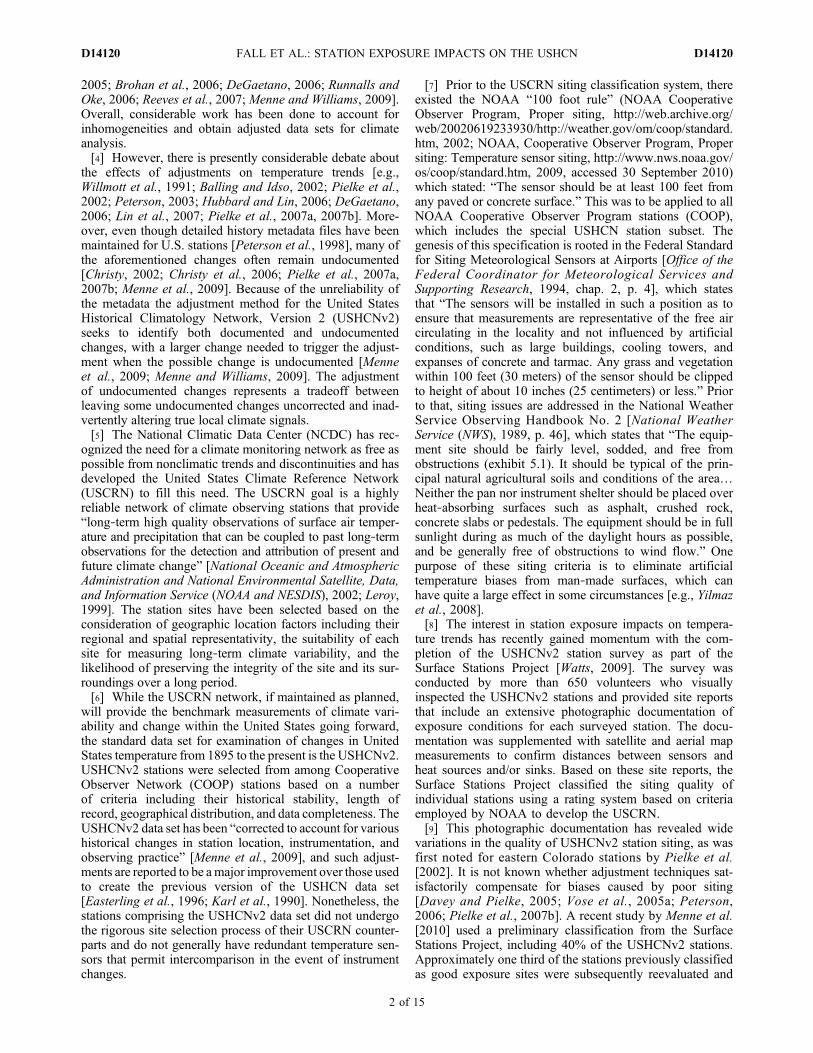
[12] We make use of the subset of USHCNv2 data fromstations whose sites were initially classified by Watts [2009]and further refined in quality control reviews led by two ofus (Jones and Watts), using the USCRN site selectionclassification scheme for temperature and humidity mea-surements [NOAA and NESDIS, 2002], originally developedby Leroy [1999] (Table 1). The site surveys were per-formed between 2 June 2007 and 23 February 2010, and1007 stations (82.5% of the USHCN network) were classi-fied (Figure 1). Any known changes in siting characteristicsafter that period are ignored.[13] In the early phase of the project, the easiest stations to

locate were near population centers (shortest driving dis-tances), this early data set with minimal quality control had adisproportionate bias toward urban stations and only ahandful of CRN1/2 stations existed in that preliminary dataset. In addition, the project had to deal with a number ofproblems including (1) poor quality of metadata archived atNCDC for the NWS managed COOP stations; (2) no flagfor specific COOP stations as being part of the USHCNsubset; (3) some station observers not knowing whethertheir station was USHCN or not; and (4) NCDC‐archivedmetadata often lagging station moves (when a curator diedfor example) as much as a year. As a result, the identifica-tion of COOP stations was difficult, sometimes necessitatingresurveying the area to get the correct COOP station thatwas part of the USHCN network. Whenever it was deter-mined that a station had been misidentified, the survey wasdone again. In January 2010, NCDC added a USHCN flagto the metadata description, making it easier to performquality control checks for station identification. NCDC hasalso now archived accurate metadata GPS information forstation coordinates, making it possible to accurately checkstation placement using aerial photography and GoogleEarth imagery. Three quality control passes to ensure stationidentification, thermometer placement, and distances toobjects and heat sinks were done by a two person team. Thetwo quality control team members had to agree with theirassessment, and with the findings of the volunteer for thestation. If not, the station was assigned for resurvey and thenincluded if the resurvey met quality control criteria. Atpresent, the project has surveyed well in excess of 87% ofthe network, but only those surveys that met quality controlrequirements are used in this paper, namely 82.5% of the1221 USHCN stations.[14] In addition to station ratings, the surveys provided an

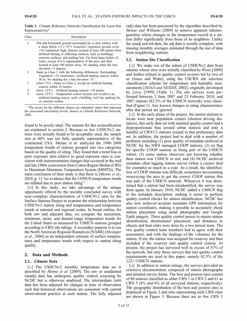
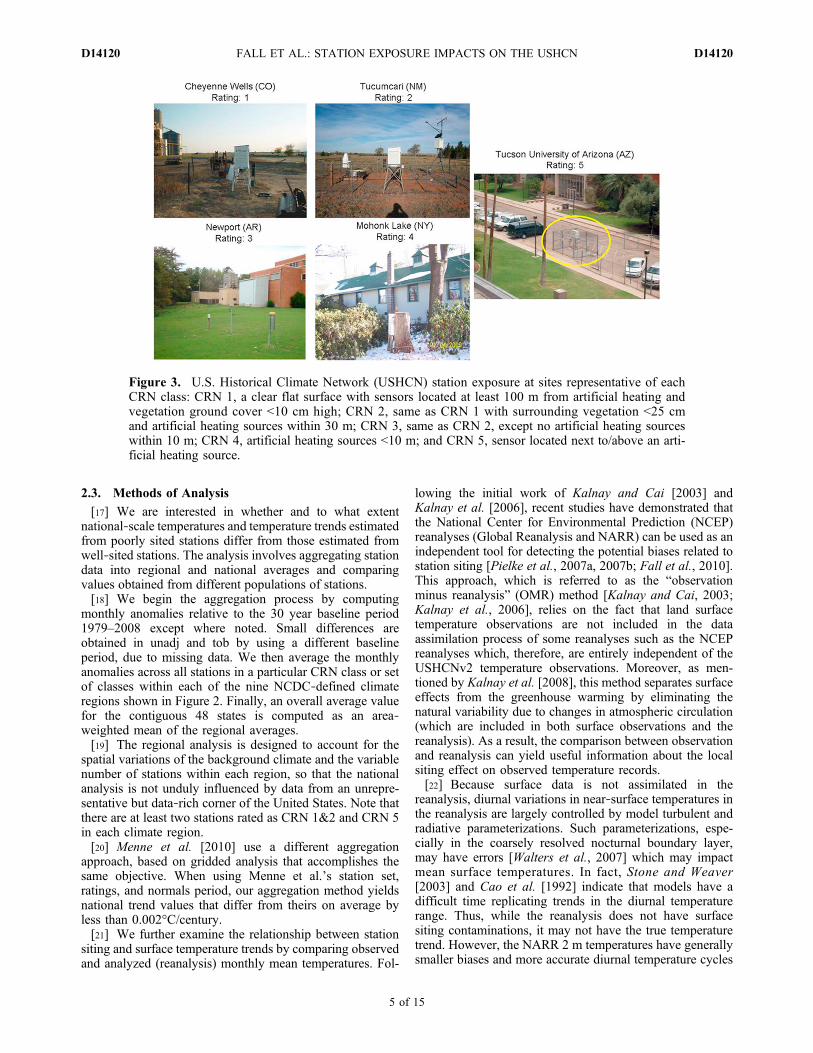
extensive documentation composed of station photographsand detailed survey forms. The best and poorest sites consistof 80 stations classified as either CRN 1 or CRN 2 and 61 asCRN 5 (8% and 6% of all surveyed stations, respectively).The geographic distribution of the best and poorest sites isdisplayed in Figure 2 and sites representing each CRN classare shown in Figure 3. Because there are so few CRN 1

Table 1. Climate Reference Network Classification for Local SiteRepresentativitya

Class Description

1 Flat and horizontal ground surrounded by a clear surface witha slope below 1/3 (<19°). Grass/low vegetation ground cover<10 centimeters high. Sensors located at least 100 meters fromartificial heating or reflecting surfaces, such as buildings,concrete surfaces, and parking lots. Far from large bodies ofwater, except if it is representative of the area, and thenlocated at least 100 meters away. No shading when the Sunelevation >3 degrees.

2 Same as Class 1 with the following differences. SurroundingVegetation <25 centimeters. Artificial heating sources within30 m. No shading for a Sun elevation >5°.

3 (error 1°C) ‐ Same as Class 2, except no artificial heatingsources within 10 meters.

4 (error ≥2°C) ‐ Artificial heating sources <10 meters5 (error ≥5°C) ‐ Temperature sensor located next to/above an

artificial heating source, such a building, roof top, parking lot,or concrete surface

aThe errors for the different classes are estimated values that representthe associated uncertainty levels. Source is Climate Reference Network,2002.


3 of 15

sites, we treat sites rated as CRN 1 and CRN 2 as belongingto the single class CRN 1&2. These would also be stationsthat meet the older NOAA/NWS “100 foot rule” (∼30 m) forCOOP stations.[15] The CRN 1&2 and CRN 5 classes are not evenly

distributed across the lower 48 states or within many indi-vidual climate regions. In order to test the sensitivity ofresults to this uneven distribution, we create two sets of“proxy” stations for the CRN 1&2 and CRN 5 stations. Theproxy stations are the nearest CRN 3 or CRN 4 class stationsto the CRN 1&2 and CRN 5 stations, except that proxiesmust be within the same climate region and cannot simul-taneously represent two CRN 1&2 or two CRN 5 stations.The proxy stations thus mimic the geographical distributionof the stations they are paired with. The CRN 1&2 proxieshave a slightly greater proportion of CRN 3 stations than dothe CRN 5 proxies (31% versus 26%), but this difference insiting characteristics is expected to be too small to affect theanalyses.

[16] A match between temperatures or trends calculatedfrom CRN 1&2 proxies and the complete set of CRN 3 and4 stations implies that the irregular distribution of CRN 1&2stations does not affect the temperature or trend calculations.Conversely, if the calculations using CRN 1&2 stations andCRN 1&2 proxy stations differ in the same manner fromcalculations using CRN 3 and 4 stations, geographical dis-tribution rather than station siting characteristics is impli-cated as the cause of the difference between CRN 1&2 andCRN 3/CRN 4 calculations. Similar comparisons may bemade between CRN 5 and CRN 3/CRN 4 using the CRN 5proxies. Differences between CRN 1&2 and CRN 5 tem-perature and trend estimates are likely to be due to poorgeographical sampling if their proxies also produce differenttemperature and trend estimates, while they are likely to bedue to siting and associated characteristics if estimates fromtheir proxies match estimates from the complete pool ofCRN 3 and CRN 4 stations.

Figure 1. Surveyed USHCN surface stations. The site quality ratings assigned by the Surface StationsProject are based on criteria utilized in site selection for the Climate Reference Network (CRN). Temper-ature errors represent the additional estimated uncertainty added by siting [Leroy, 1999; NOAA andNESDIS, 2002].

Figure 2. Distribution of good exposure (Climate Reference Network (CRN) rating = 1 and 2) and badexposure (CRN = 5) sites. The ratings are based on classifications by Watts [2009] using the CRN siteselection rating shown in Table 1. The stations are displayed with respect to the nine climate regionsdefined by NCDC.


4 of 15

2.3. Methods of Analysis

[17] We are interested in whether and to what extentnational‐scale temperatures and temperature trends estimatedfrom poorly sited stations differ from those estimated fromwell‐sited stations. The analysis involves aggregating stationdata into regional and national averages and comparingvalues obtained from different populations of stations.[18] We begin the aggregation process by computing

monthly anomalies relative to the 30 year baseline period1979–2008 except where noted. Small differences areobtained in unadj and tob by using a different baselineperiod, due to missing data. We then average the monthlyanomalies across all stations in a particular CRN class or setof classes within each of the nine NCDC‐defined climateregions shown in Figure 2. Finally, an overall average valuefor the contiguous 48 states is computed as an area‐weighted mean of the regional averages.[19] The regional analysis is designed to account for the

spatial variations of the background climate and the variablenumber of stations within each region, so that the nationalanalysis is not unduly influenced by data from an unrepre-sentative but data‐rich corner of the United States. Note thatthere are at least two stations rated as CRN 1&2 and CRN 5in each climate region.[20] Menne et al. [2010] use a different aggregation

approach, based on gridded analysis that accomplishes thesame objective. When using Menne et al.’s station set,ratings, and normals period, our aggregation method yieldsnational trend values that differ from theirs on average byless than 0.002°C/century.[21] We further examine the relationship between station

siting and surface temperature trends by comparing observedand analyzed (reanalysis) monthly mean temperatures. Fol-

lowing the initial work of Kalnay and Cai [2003] andKalnay et al. [2006], recent studies have demonstrated thatthe National Center for Environmental Prediction (NCEP)reanalyses (Global Reanalysis and NARR) can be used as anindependent tool for detecting the potential biases related tostation siting [Pielke et al., 2007a, 2007b; Fall et al., 2010].This approach, which is referred to as the “observationminus reanalysis” (OMR) method [Kalnay and Cai, 2003;Kalnay et al., 2006], relies on the fact that land surfacetemperature observations are not included in the dataassimilation process of some reanalyses such as the NCEPreanalyses which, therefore, are entirely independent of theUSHCNv2 temperature observations. Moreover, as men-tioned by Kalnay et al. [2008], this method separates surfaceeffects from the greenhouse warming by eliminating thenatural variability due to changes in atmospheric circulation(which are included in both surface observations and thereanalysis). As a result, the comparison between observationand reanalysis can yield useful information about the localsiting effect on observed temperature records.[22] Because surface data is not assimilated in the

reanalysis, diurnal variations in near‐surface temperatures inthe reanalysis are largely controlled by model turbulent andradiative parameterizations. Such parameterizations, espe-cially in the coarsely resolved nocturnal boundary layer,may have errors [Walters et al., 2007] which may impactmean surface temperatures. In fact, Stone and Weaver[2003] and Cao et al. [1992] indicate that models have adifficult time replicating trends in the diurnal temperaturerange. Thus, while the reanalysis does not have surfacesiting contaminations, it may not have the true temperaturetrend. However, the NARR 2 m temperatures have generallysmaller biases and more accurate diurnal temperature cycles

Figure 3. U.S. Historical Climate Network (USHCN) station exposure at sites representative of eachCRN class: CRN 1, a clear flat surface with sensors located at least 100 m from artificial heating andvegetation ground cover <10 cm high; CRN 2, same as CRN 1 with surrounding vegetation <25 cmand artificial heating sources within 30 m; CRN 3, same as CRN 2, except no artificial heating sourceswithin 10 m; CRN 4, artificial heating sources <10 m; and CRN 5, sensor located next to/above an arti-ficial heating source.


5 of 15

than previous reanalysis products, as shown by Mesingeret al. [2006] and in recent studies [e.g., Pielke et al., 2007a].[23] Because there may be systematic biases in both

NARR temperatures and NARR temperature trends, theNARR temperatures are used here in a way that minimizesor removes the effect of such biases. The only assumptionmade is that any NARR temperature biases or temperaturetrend biases at USHCNv2 station locations are independentof the microscale siting characteristics of the USHCNv2stations. This seems plausible: since USHCNv2 temperaturedata is not ingested into NARR, there is no way that NARRcan be directly affected by USHCNv2 microscale sitingcharacteristics.[24] We bilinearly interpolate the NARR gridded mean

temperatures for every month within the period 1979–2008to USHCNv2 locations and subtract them from theUSHCNv2 values of maximum, average, and minimumtemperature prior to computation of monthly anomalies andaggregation. The resulting anomaly values are then aggre-gated to the lower 48 states in the same manner as describedabove for the USHCNv2 trends. This procedure effectivelyproduces an estimate of the average temperature across theUnited States based upon particular classes of USHCNv2observations, using the NARR mean temperatures as a firstguess field. The NARR mean temperatures are not definedin the same way as USHCNv2 average temperatures. How-ever, systematic differences among CRN classes in analyzedobserved minus NARR temperatures will be due to thesurface station characteristics, not to the NARR temperaturecomputation. The possibility of random NARR errors pro-ducing a false signal is addressed through the Monte Carloresampling described below, and the possibility of regionalvariations of NARR errors producing a false signal isaddressed through comparisons with proxy stations.[25] The statistical significance of differences in tem-

peratures and temperature trends of stations within a par-ticular target CRN class relative to CRN 1&2 is estimatedusing Monte Carlo resampling. The assignments of stationsto the target class and to class 1&2 are permuted randomly,under the constraint that at least two stations of each classmust remain in each NCDC climate region, and valuesrecomputed. For example, there are 80 CRN 1&2 stationsand 61 CRN 5 stations. These stations are randomly rear-ranged to produce random groups of 80 and 61 stations. Thetwo groups are checked to see if there are at least two sta-tions of each group within each climate region. If so, cal-culation of means and/or trends proceeds as described abovefor the true CRN classes. This procedure is carried out untilthere are 10,000 realizations of means and/or trends, and thenull hypothesis that differences are independent of CRNclassification is rejected at the 95% confidence level if thetwo‐sided p value of the observed difference is less than 0.05.[26] Differences that depend upon CRN classification may

be due specifically to the station siting characteristics or bedue to other characteristics that covary with station siting,such as instrument type. Siting differences directly affecttemperature trends if the poor siting compromises trendmeasurements or if changes in siting have led to artificialdiscontinuities. In what follows, to the extent that significantdifferences are found among classes, the well‐sited stationswill be assumed to have more accurate measurements oftemperature and temperature trends. We plan to investigate

the various possible covarying causes for the dependence ofclimate data quality on siting classification in a separatepaper.

3. Trend Analysis

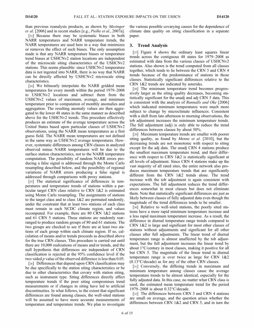
[27] Figure 4 shows the ordinary least squares lineartrends across the contiguous 48 states for 1979–2008 asestimated with data from the various classes of USHCNv2stations. Also shown is the trend computed from all classestogether, which tends to lie between the CRN 3 and CRN 4trends because of the predominance of stations in thoseclasses. Statistically significant differences relative to theCRN 1&2 trends are indicated by asterisks.[28] The minimum temperature trend becomes progres-

sively larger as the siting quality decreases, becoming sta-tistically significant for the unadj and adj CRN 5 data. Thisis consistent with the analysis of Runnalls and Oke [2006]which indicated minimum temperatures were much moresubject to change by microclimate influences. Consistentwith a shift from late afternoon to morning observations, thetob adjustment increases the minimum temperature trends.The full adjustment (adj) is only able to reduce the trenddifferences between classes by about 50%.[29] Maximum temperature trends are smaller with poorer

siting quality, as found by Menne et al. [2010], but thedecreasing trends are not monotonic with respect to sitingexcept for the adj data. The unadj CRN 4 stations producethe smallest maximum temperature trend, and their differ-ence with respect to CRN 1&2 is statistically significant atall levels of adjustment. Since CRN 4 stations make up thevast majority of all rated sites, the entire network also pro-duces maximum temperature trends that are significantlydifferent from the CRN 1&2 trends alone. The trendincrease with the tob adjustment is again consistent withexpectations. The full adjustment reduces the trend differ-ences somewhat in most classes but does not eliminatethem. Note that statistically significant differences are just aslikely between classes of fully adjusted data even though themagnitude of the trend differences tends to be smaller.[30] Relative to well‐sited stations, the poorly sited sta-

tions have a more rapid minimum temperature increase anda less rapid maximum temperature increase. As a result, thedifference in diurnal temperature range trends compared toCRN 1&2 is large and significant for most other classes ofstations without adjustments and significant for all otherclasses after full adjustments. The linear trend of diurnaltemperature range is almost unaffected by the tob adjust-ment, but the full adjustment increases the linear trend byabout 1°C/century in most classes, making it positive for allbut CRN 5. The magnitude of the linear trend in diurnaltemperature range is over twice as large for CRN 1&2(0.13°C/decade) as for any of the other CRN classes.[31] Conversely, the differing trends in maximum and

minimum temperature among classes cause the averagetemperature trends to be almost identical, especially for thefully adjusted data. In this case, no matter what CRN class isused, the estimated mean temperature trend for the period1979–2008 is about 0.32°C/decade.[32] The differences between CRN 3 and CRN 4 stations

are small on average, and the question arises whether thedifferences between CRN 1&2 and CRN 5, and in turn the


6 of 15

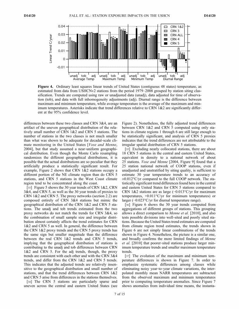
differences between these two classes and CRN 3&4, are anartifact of the uneven geographical distribution of the rela-tively small number of CRN 1&2 and CRN 5 stations. Thenumber of stations in the two classes is not much smallerthan what was shown to be adequate for decadal‐scale cli-mate monitoring in the United States [Vose and Menne,2004], but that study assumed a near‐uniform geographi-cal distribution. Even though the Monte Carlo resamplingrandomizes the different geographical distributions, it ispossible that the actual distributions are so peculiar that theyartificially produce a statistically significant result. Forexample, Figure 2 shows that CRN 1&2 stations occupy adifferent portion of the NE climate region than do CRN 5stations, and CRN 5 stations in the West Coast climateregion tend to be concentrated along the coast.[33] Figure 5 shows the 30 year trends of CRN 1&2, CRN

3&4, and CRN 5, as well as the 30 year trends of proxies toCRN 1&2 and CRN 5. The proxy networks (section 2.2) arecomposed entirely of CRN 3&4 stations but mimic thegeographical distribution of the CRN 1&2 and CRN 5 sta-tions. The unadj and tob trends estimated from the twoproxy networks do not match the trends for CRN 3&4, sothe combination of small sample size and irregular distri-bution almost certainly affects the trend estimates for CRN1&2 and CRN 5 as well. In general, the difference betweenthe CRN 1&2 proxy trends and the CRN 5 proxy trends hasthe same sign but smaller magnitude than the differencebetween the real CRN 1&2 trends and CRN 5 trends,implying that the geographical distribution of stations iscontributing to the unadj and tob differences between CRN1&2 and CRN 5. For the adj trends, though, the proxytrends are consistent with each other and with the CRN 3&4trends, and differ from the CRN 1&2 and CRN 5 trends.This indicates that the adjusted trends are relatively insen-sitive to the geographical distribution and small number ofstations, and that the trend differences between CRN 1&2and CRN 5 arise from differences in the stations themselves.[34] The CRN 5 stations are particularly sparse and

uneven across the central and eastern United States (see

Figure 2). Nonetheless, the fully adjusted trend differencesbetween CRN 1&2 and CRN 5 computed using only sta-tions in climate regions 1 through 6 are still large enough tobe statistically significant, and analysis of CRN 5 proxiesindicates that the trend differences are not attributable to theirregular spatial distribution of CRN 5 stations.[35] Excluding nearly collocated stations, there are about

18 CRN 5 stations in the central and eastern United States,equivalent in density to a national network of about25 stations. Vose and Menne [2004, Figure 9] found that a25 station national network of COOP stations, even ifunadjusted and unstratified by siting quality, is sufficient toestimate 30 year temperature trends to an accuracy of±0.012°C/yr compared to the full COOP network. The sta-tistically significant trend differences found here in the centraland eastern United States for CRN 5 stations compared toCRN 1&2 stations are as large (−0.013°C/yr for maximumtemperatures, +0.011°C/yr for minimum temperatures) orlarger (−0.023°C/yr for diurnal temperature range).[36] Figure 6 shows the 30 year trends computed from

aggregations of different groups of stations. This groupingallows a direct comparison to Menne et al. [2010], and alsotests possible divisions into well‐sited and poorly sited sta-tions. Because the United States trend estimates are computedfrom climate region trend estimates, the trends shown inFigure 6 are not simply linear combinations of the trendsshown in Figure 4. Nonetheless, the picture is a similar one,and broadly confirms the more limited findings of Menneet al. [2010] that poorer‐sited stations produce larger min-imum temperature trends and smaller maximum temperaturetrends.[37] The evolution of the maximum and minimum tem-

perature differences is shown in Figure 7. In order toemphasize systematic differences among classes whileeliminating noisy year‐to‐year climate variations, the inter-polated monthly mean NARR temperatures are subtractedfrom the observed maximum and minimum temperaturesprior to computing temperature anomalies. Since Figure 7shows anomalies from individual time means, the instanta-

Figure 4. Ordinary least squares linear trends of United States (contiguous 48 states) temperature, asestimated from data from USHCNv2 stations from the period 1979–2008 grouped by station siting clas-sification. Trends are computed using raw or unadjusted data (unadj), data adjusted for time of observa-tion (tob), and data with full inhomogeneity adjustments (adj). Diurnal range is the difference betweenmaximum and minimum temperature, while average temperature is the average of the maximum and min-imum temperatures. Asterisks indicate that trend differences relative to CRN 1&2 are significantly differ-ent at the 95% confidence level.


7 of 15

neous differences between classes are not as important asthe changes in those differences over time. In particular,systematic differences among the different classes changedramatically around 1984–1987. This is coincident with awidespread transition to MMTS thermometers at most sta-tions. In a field test, the MMTS recorded cooler maximumtemperatures by about 0.4 C and warmer minimum tem-peratures by about 0.2 C than did a thermometer housed in aCotton Region Shelter (CRS) [Wendland and Armstrong,1993]. However, the instrumentation change at COOP sta-tions was typically synchronous with a change in the sitingcharacteristics [Menne et al., 2010]. The combined effect ofthe MMTS transition and simultaneous siting changes wasan average maximum temperature decrease of 0.4 C andminimum temperature increase of 0.3 C relative to CRSstations [Quayle et al., 1991], similar to what might beexpected from the instrumentation change alone, but theactual discontinuity varied widely from station to station[Hubbard and Lin, 2006], indicating that the micrositechanges were similarly important on a station by stationbasis.[38] Between‐class temperature differences do not remain

stable after the primary MMTS transition period. The extentto which this is due to siting classifications compared toimperfect estimations of United States temperature changes

is shown in Figure 8, which breaks down the differencebetween CRN 1&2 and CRN 5 temperatures as CRN 1&2and their proxies, CRN 5 and their proxies, and the differ-ences between the two sets of proxies. The latter differenceshould account for most of the representativeness error dueto the small number of stations in each class and regionallydependent estimation errors associated with NARR, therebyisolating effects directly associated with siting. As withFigure 7, the important features are the changes in the dif-ferences over time.[39] Besides the transition in the mid‐1980s discussed

earlier, the difference in minimum tob temperatures esti-mated from the two CRN groups (Figure 8a) changes byabout −0.2°C around the year 2000. The mid‐1980s changearises from both CRN 1&2/proxy differences and differ-ences between the two proxy sets, while the 2000 changearises mainly from the CRN 5/proxy differences. The fulladjustment (Figure 8b) reduces the change in differences, butthe remaining change is primarily due to the CRN 5/proxydifferences as the other two differences are stable over time.Most, but not all, of the CRN 5/proxy change remaining afterfull adjustments is in the mid‐1980s.[40] The difference inmaximum tob temperatures (Figure 8c)

has even more dramatic changes, climbing to a maximum inthe mid‐1990s and falling thereafter. Because the difference

Figure 5. Linear trends of United States (contiguous 48 states) temperature, as in Figure 4, but for thestation classifications shown. The proxy networks are nearest‐neighbor networks to CRN 1&2 or CRN 5stations and are composed of a mix of CRN 3 and CRN 4 stations. See text for details.

Figure 6. Linear trends of United States (contiguous 48 states) temperature, as in Figure 4, but for thestation classification groupings shown.


8 of 15

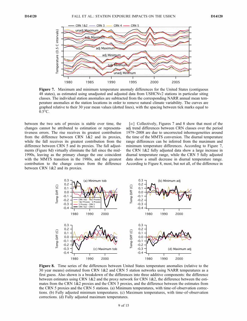
between the two sets of proxies is stable over time, thechanges cannot be attributed to estimation or representa-tiveness errors. The rise receives its greatest contributionfrom the difference between CRN 1&2 and its proxies,while the fall receives its greatest contribution from thedifference between CRN 5 and its proxies. The full adjust-ments (Figure 8d) virtually eliminate the fall since the mid‐1990s, leaving as the primary change the one coincidentwith the MMTS transition in the 1980s, and the greatestcontribution to the change comes from the differencebetween CRN 1&2 and its proxies.

[41] Collectively, Figures 7 and 8 show that most of theadj trend differences between CRN classes over the period1979–2008 are due to uncorrected inhomogeneities aroundthe time of the MMTS conversion. The diurnal temperaturerange differences can be inferred from the maximum andminimum temperature differences. According to Figure 7,the CRN 1&2 fully adjusted data show a large increase indiurnal temperature range, while the CRN 5 fully adjusteddata show a small decrease in diurnal temperature range.According to Figure 8, most, but not all, of the difference in

Figure 7. Maximum and minimum temperature anomaly differences for the United States (contiguous48 states), as estimated using unadjusted and adjusted data from USHCNv2 stations in particular sitingclasses. The individual station anomalies are subtracted from the corresponding NARR annual mean tem-perature anomalies at the station locations in order to remove natural climate variability. The curves aregraphed relative to their 30 year mean values (dotted lines), with the spacing between tick marks equal to0.5°C.

Figure 8. Time series of the differences between United States temperature anomalies (relative to the30 year means) estimated from CRN 1&2 and CRN 5 station networks using NARR temperatures as afirst guess. Also shown is a breakdown of the differences into three additive components: the differencebetween estimates using CRN 1&2 and the proxy network for CRN 1&2, the difference between the esti-mates from the CRN 1&2 proxies and the CRN 5 proxies, and the difference between the estimates fromthe CRN 5 proxies and the CRN 5 stations. (a) Minimum temperatures, with time‐of‐observation correc-tions. (b) Fully adjusted minimum temperatures. (c) Maximum temperatures, with time‐of‐observationcorrections. (d) Fully adjusted maximum temperatures.


9 of 15

diurnal temperature range estimated from the two classesarises during the mid to late 1980s.[42] The differences in temperature trends among

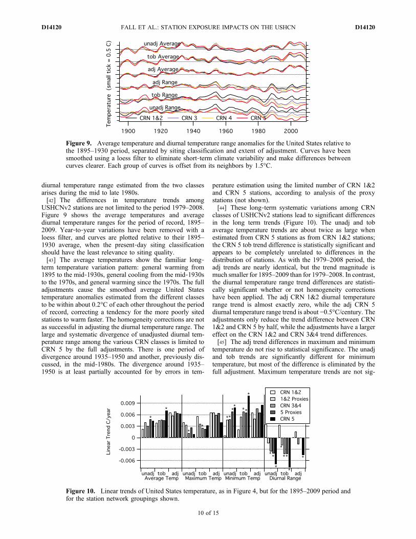
USHCNv2 stations are not limited to the period 1979–2008.Figure 9 shows the average temperatures and averagediurnal temperature ranges for the period of record, 1895–2009. Year‐to‐year variations have been removed with aloess filter, and curves are plotted relative to their 1895–1930 average, when the present‐day siting classificationshould have the least relevance to siting quality.[43] The average temperatures show the familiar long‐

term temperature variation pattern: general warming from1895 to the mid‐1930s, general cooling from the mid‐1930sto the 1970s, and general warming since the 1970s. The fulladjustments cause the smoothed average United Statestemperature anomalies estimated from the different classesto be within about 0.2°C of each other throughout the periodof record, correcting a tendency for the more poorly sitedstations to warm faster. The homogeneity corrections are notas successful in adjusting the diurnal temperature range. Thelarge and systematic divergence of unadjusted diurnal tem-perature range among the various CRN classes is limited toCRN 5 by the full adjustments. There is one period ofdivergence around 1935–1950 and another, previously dis-cussed, in the mid‐1980s. The divergence around 1935–1950 is at least partially accounted for by errors in tem-

perature estimation using the limited number of CRN 1&2and CRN 5 stations, according to analysis of the proxystations (not shown).[44] These long‐term systematic variations among CRN

classes of USHCNv2 stations lead to significant differencesin the long term trends (Figure 10). The unadj and tobaverage temperature trends are about twice as large whenestimated from CRN 5 stations as from CRN 1&2 stations;the CRN 5 tob trend difference is statistically significant andappears to be completely unrelated to differences in thedistribution of stations. As with the 1979–2008 period, theadj trends are nearly identical, but the trend magnitude ismuch smaller for 1895–2009 than for 1979–2008. In contrast,the diurnal temperature range trend differences are statisti-cally significant whether or not homogeneity correctionshave been applied. The adj CRN 1&2 diurnal temperaturerange trend is almost exactly zero, while the adj CRN 5diurnal temperature range trend is about −0.5°C/century. Theadjustments only reduce the trend difference between CRN1&2 and CRN 5 by half, while the adjustments have a largereffect on the CRN 1&2 and CRN 3&4 trend differences.[45] The adj trend differences in maximum and minimum

temperature do not rise to statistical significance. The unadjand tob trends are significantly different for minimumtemperature, but most of the difference is eliminated by thefull adjustment. Maximum temperature trends are not sig-

Figure 9. Average temperature and diurnal temperature range anomalies for the United States relative tothe 1895–1930 period, separated by siting classification and extent of adjustment. Curves have beensmoothed using a loess filter to eliminate short‐term climate variability and make differences betweencurves clearer. Each group of curves is offset from its neighbors by 1.5°C.

Figure 10. Linear trends of United States temperature, as in Figure 4, but for the 1895–2009 period andfor the station network groupings shown.


10 of 15

nificantly different except for tob trend differences betweenCRN 1&2 and CRN 3&4.[46] Not only are the trends themselves smaller, but the

1895–2009 differences between CRN 1&2 and CRN 5trends are also smaller than the corresponding 1979–2008trend differences. This implies that, to the extent that the trenddifferences are caused by siting changes, a large portion ofthe siting changes has taken place since 1979. Nonetheless,Figure 9 shows that the diurnal temperature range trend wasconsistently lower for stations presently classified as morepoorly sited from about 1920 onward.[47] We computed the variance of the detrended aggre-

gated monthly anomaly time series from stations of differentclasses and the correlation coefficients between the aggre-gated monthly anomalies and the NARR monthly anomaliesaggregated from station sites to determine whether the sitingdifferences influenced estimates of climate variability acrossthe United States on an annual time scale. No statisticallysignificant variance or correlation differences were found.

4. Temperature Bias Analysis

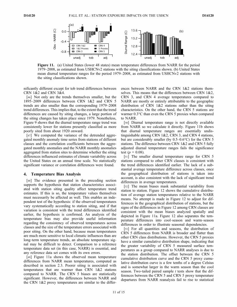
[48] The evidence presented in the preceding sectionsupports the hypothesis that station characteristics associ-ated with station siting quality affect temperature trendestimates. If this is so, the temperature values themselvesmust necessarily be affected as well. This enables an inde-pendent test of the hypothesis: if the observed temperaturesvary systematically according to station siting, and if thatvariation is consistent with the trend differences identifiedearlier, the hypothesis is confirmed. An analysis of thetemperature bias may also provide useful informationregarding the consistency of observed temperatures acrossclasses and the size of the temperature errors associated withpoor siting. On the other hand, because mean temperaturesare much more sensitive to local climatic influences than arelong‐term temperature trends, an absolute temperature sig-nal may be difficult to detect. Comparison to a referencetemperature data set (in this case, NARR) is essential, andany reference data set comes with its own errors.[49] Figure 11a shows the observed mean temperature

differences from NARR mean temperatures, computed asdescribed in section 2.3. Poorer siting is associated withtemperatures that are warmer than CRN 1&2 stationscompared to NARR. The CRN 5 biases are statisticallysignificant. However, the differences between NARR andthe CRN 1&2 proxy temperatures are similar to the differ-

ences between NARR and the CRN 1&2 stations them-selves. This means that the differences between CRN 1&2,CRN 3, and CRN 4 average temperatures compared toNARR are mostly or entirely attributable to the geographicdistribution of CRN 1&2 stations rather than the sitingcharacteristics. On the other hand, the CRN 5 stations arewarmer 0.3°C than even the CRN 5 proxies when comparedto NARR.[50] Diurnal temperature range is not directly available

from NARR so we calculate it directly. Figure 11b showsthat diurnal temperature ranges are essentially undis-tinguishable among CRN 1&2, CRN 3, and CRN 4 stations,but are considerably smaller (by 0.5–0.6°C) for the CRN 5stations. The difference between CRN 1&2 and CRN 5 fullyadjusted diurnal temperature ranges fails the significancetest (p = 0.08).[51] The smaller diurnal temperature range for CRN 5

stations compared to other CRN classes is consistent withthe trend differences identified earlier. The lack of a sub-stantial average temperature difference across classes, oncethe geographical distribution of stations is taken intoaccount, is also consistent with the lack of significant trenddifferences in average temperatures.[52] The mean biases mask substantial variability from

station to station. Figure 12 shows the cumulative distribu-tion of average station temperatures relative to the NARRmeans. No attempt is made in Figure 12 to adjust for dif-ferences in the geographical distribution of stations, but thesigns of the differences in Figure 12 among CRN classes areconsistent with the mean biases analyzed spatially anddepicted in Figure 11a. Figure 12 also separates the tem-perature differences into cool‐season and warm‐seasondifferences in order to illustrate seasonal dependencies.[53] For all quantities and seasons, the distribution of

CRN 5 differences from NARR is broader and flatter thanother CRN class distributions. However, the CRN 5 proxieshave a similar cumulative distribution shape, indicating thatthe greater variability of CRN 5 measured surface tem-peratures as a group compared to NARR analyses is due tothe station distribution. The offset between the CRN 5cumulative distribution curve and the CRN 5 proxy cumu-lative distribution curve is a few tenths of a degree Celsiusand is somewhat larger in the warm season than the coolseason. Two‐tailed paired sample t tests show that the dif-ferences between the CRN 5 and CRN 5 proxy temperaturedepartures from NARR reanalysis fail to rise to statistical

Figure 11. (a) United States (lower 48 states) mean temperature differences from NARR for the period1979–2008, as estimated from USHCNv2 stations with the siting classifications shown. (b) United Statesmean diurnal temperature ranges for the period 1979–2008, as estimated from USHCNv2 stations withthe siting classifications shown.


11 of 15

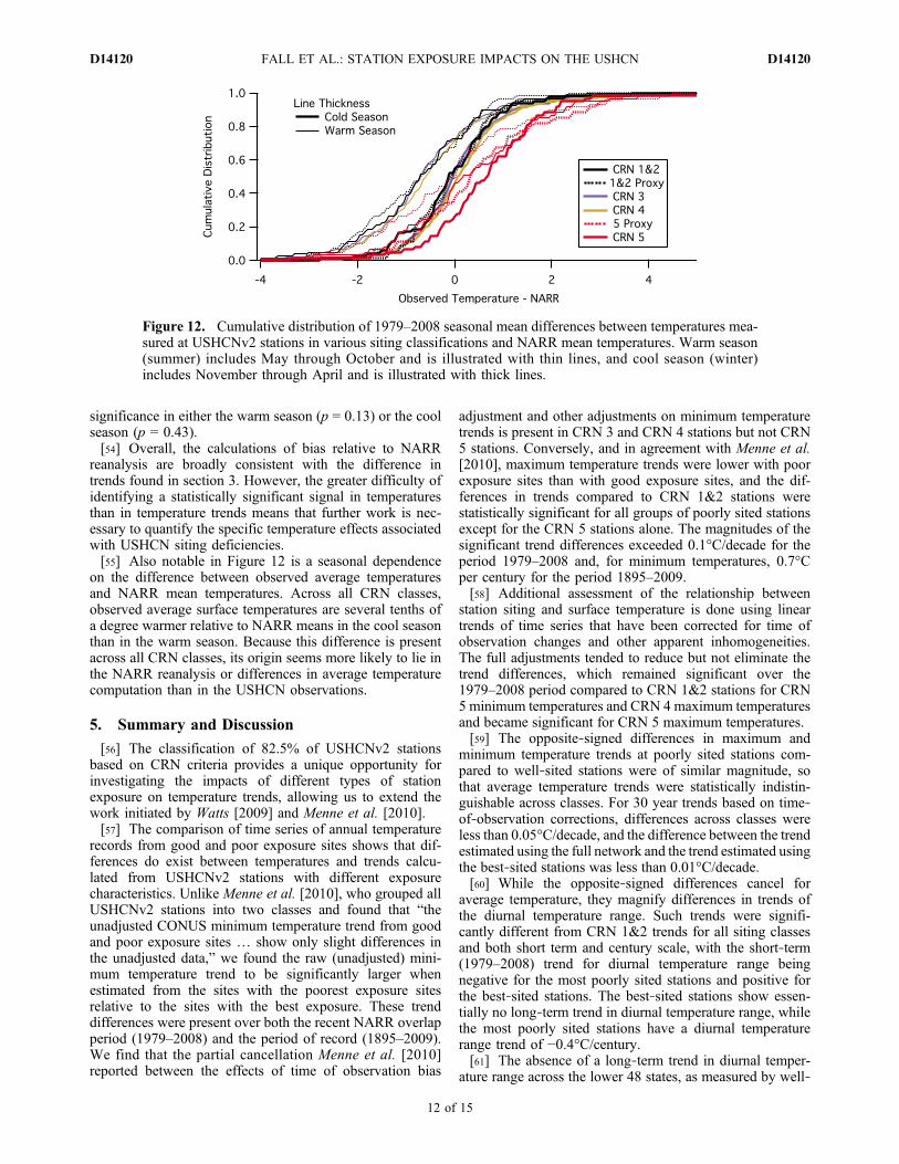
significance in either the warm season (p = 0.13) or the coolseason (p = 0.43).[54] Overall, the calculations of bias relative to NARR

reanalysis are broadly consistent with the difference intrends found in section 3. However, the greater difficulty ofidentifying a statistically significant signal in temperaturesthan in temperature trends means that further work is nec-essary to quantify the specific temperature effects associatedwith USHCN siting deficiencies.[55] Also notable in Figure 12 is a seasonal dependence

on the difference between observed average temperaturesand NARR mean temperatures. Across all CRN classes,observed average surface temperatures are several tenths ofa degree warmer relative to NARR means in the cool seasonthan in the warm season. Because this difference is presentacross all CRN classes, its origin seems more likely to lie inthe NARR reanalysis or differences in average temperaturecomputation than in the USHCN observations.

5. Summary and Discussion

[56] The classification of 82.5% of USHCNv2 stationsbased on CRN criteria provides a unique opportunity forinvestigating the impacts of different types of stationexposure on temperature trends, allowing us to extend thework initiated by Watts [2009] and Menne et al. [2010].[57] The comparison of time series of annual temperature

records from good and poor exposure sites shows that dif-ferences do exist between temperatures and trends calcu-lated from USHCNv2 stations with different exposurecharacteristics. Unlike Menne et al. [2010], who grouped allUSHCNv2 stations into two classes and found that “theunadjusted CONUS minimum temperature trend from goodand poor exposure sites … show only slight differences inthe unadjusted data,” we found the raw (unadjusted) mini-mum temperature trend to be significantly larger whenestimated from the sites with the poorest exposure sitesrelative to the sites with the best exposure. These trenddifferences were present over both the recent NARR overlapperiod (1979–2008) and the period of record (1895–2009).We find that the partial cancellation Menne et al. [2010]reported between the effects of time of observation bias

adjustment and other adjustments on minimum temperaturetrends is present in CRN 3 and CRN 4 stations but not CRN5 stations. Conversely, and in agreement with Menne et al.[2010], maximum temperature trends were lower with poorexposure sites than with good exposure sites, and the dif-ferences in trends compared to CRN 1&2 stations werestatistically significant for all groups of poorly sited stationsexcept for the CRN 5 stations alone. The magnitudes of thesignificant trend differences exceeded 0.1°C/decade for theperiod 1979–2008 and, for minimum temperatures, 0.7°Cper century for the period 1895–2009.[58] Additional assessment of the relationship between

station siting and surface temperature is done using lineartrends of time series that have been corrected for time ofobservation changes and other apparent inhomogeneities.The full adjustments tended to reduce but not eliminate thetrend differences, which remained significant over the1979–2008 period compared to CRN 1&2 stations for CRN5 minimum temperatures and CRN 4 maximum temperaturesand became significant for CRN 5 maximum temperatures.[59] The opposite‐signed differences in maximum and

minimum temperature trends at poorly sited stations com-pared to well‐sited stations were of similar magnitude, sothat average temperature trends were statistically indistin-guishable across classes. For 30 year trends based on time‐of‐observation corrections, differences across classes wereless than 0.05°C/decade, and the difference between the trendestimated using the full network and the trend estimated usingthe best‐sited stations was less than 0.01°C/decade.[60] While the opposite‐signed differences cancel for

average temperature, they magnify differences in trends ofthe diurnal temperature range. Such trends were signifi-cantly different from CRN 1&2 trends for all siting classesand both short term and century scale, with the short‐term(1979–2008) trend for diurnal temperature range beingnegative for the most poorly sited stations and positive forthe best‐sited stations. The best‐sited stations show essen-tially no long‐term trend in diurnal temperature range, whilethe most poorly sited stations have a diurnal temperaturerange trend of −0.4°C/century.[61] The absence of a long‐term trend in diurnal temper-

ature range across the lower 48 states, as measured by well‐

Figure 12. Cumulative distribution of 1979–2008 seasonal mean differences between temperatures mea-sured at USHCNv2 stations in various siting classifications and NARR mean temperatures. Warm season(summer) includes May through October and is illustrated with thin lines, and cool season (winter)includes November through April and is illustrated with thick lines.


12 of 15

sited surface stations, has not previously been noted. Paststudies of large‐scale diurnal temperature range trends, suchas by Karl et al. [1984], Easterling et al. [1997], and Voseet al. [2005b], identified a downward trend from the 1940sor 1950s to at least the 1980s, with little or no trend since.Karl et al. [1993] note that there was no downward trend inthe United States prior to the mid‐1950s. The presentanalysis confirms the multidecade downward trend begin-ning in the mid‐1950s, but finds that upward trends duringother periods resulted in zero diurnal temperature rangetrend for the period of record, 1895–2009.[62] Assessments comparing observed and analyzed (NARR)

monthly mean temperature anomalies illustrate how changesin temperature differences through time contribute to thetrend differences. Using CRN 1&2 sites as a baseline, time‐of‐observation corrected minimum temperature measure-ments at CRN 5 stations have grown increasingly warm,while corresponding maximum temperatures cooled steadilyuntil the mid‐1990s and warmed thereafter. The full inho-mogeneity adjustments reduce the rate of change of temper-ature differences but do not eliminate them except forremoval of the post‐1990s maximum temperature warming.The remaining trend differences imply that the adjustmentsdid not fully correct for changes in instrumentation andmicroclimate with the transition to MMTS temperaturesensors.[63] An initial attempt at estimating the magnitudes of the

temperature biases themselves is made by analyzing thedifferences between NARR temperatures and observedtemperatures. The CRN 5 stations are on average warmerthan the CRN 1&2 stations compared to interpolated NARRtemperatures by about 0.7°C. However, when the differinggeographical distribution of stations is taken into account,the difference attributable to siting characteristics alone isabout 0.3°C. The diurnal temperature range is smaller forCRN 5 stations than for all other station classes by about0.5°C, but this difference is not significant at the 5% level(p = 0.08).[64] In cases where no statistical significance was found,

the absence of statistical significance does not necessarilyimply a lack of influence of station siting characteristics,only that other variables, such as instrumentation differencesor local climatic differences, are important and may beresponsible for the calculated differences among classes.Conversely, statistically significant differences may in somecases be due to factors that covary with siting characteristicsrather than the specific siting characteristics themselves. Afollow‐up study is underway to distinguish and quantify theseparate effects of siting, instrumentation, urbanization, andother factors.[65] Overall, this study demonstrates that station exposure

does impact USHCNv2 temperatures. The temperaturesthemselves are warmest compared to independent analysesat the stations with the worst siting characteristics. Tem-perature trend estimates vary according to site classification,with poor siting leading to an overestimate of minimumtemperature trends and an underestimate of maximumtemperature trends, resulting in particular in a substantialdifference in estimates of the diurnal temperature rangetrends. Homogeneity adjustments are necessary and tend toreduce the trend differences, but statistically significantdifferences remain for all but average temperature trends.

[66] Trend differences tend to become progressivelylarger (and more likely to be statistically significant) assiting quality degrades, except for average temperaturetrends which are relatively insensitive to CRN classification.It seems that the accuracy of maximum and minimum trendestimates can be improved by using only better‐sited sta-tions, but the appropriate quality criterion probably variesfrom situation to situation. There is a necessary tradeoffbetween the number of stations (more stations improve thesignal‐to‐noise ratio) and the siting quality criterion (morelenient standards increase the observation biases). For thelong‐term trends considered here, the optimal network mayconsist exclusively of the CRN 1&2 stations. However,even the fully adjusted data from the highest‐quality stationsmay be affected by trend biases in lower‐quality stations inthe interval surrounding the change point [Pielke et al.,2007a]. It may be beneficial to exclude the most poorlysited stations from the adjustment procedure at better‐sitedstations.[67] We recommend that this type of comprehensive siting

study be extended to the global historical climate network[GHCN] temperature data (http://www.ncdc.noaa.gov/oa/climate/ghcn‐monthly/index.php), as part of the improve-ment in metadata and benchmarking of data adjustmentalgorithms proposed in the meeting organized by Stott andThorne [2010].

[68] Acknowledgments. The authors wish to acknowledge the manycooperative observers who unselfishly carry out COOP observations, whichare the backbone of climate monitoring. We also acknowledge the manyvolunteers who made the surfacestations.org project possible with their per-sonal time and efforts in gathering the nationwide survey. Special thanksare given to these prominent volunteers who expended special effortsand expertise in metadata collection and collation: Gary Boden, Don andLiz Healy, Eric Gamberg, John Goetz, Don Kostuch, John Slayton, TedSemon, Russell and Ellen Steele, and Barry Wise. Acknowledgment isgiven to former California State Climatologist James Goodridge, whowas inspirational with surveys he made of California COOP stations duringhis tenure. Station photographs are courtesy of Evan Jones, Warren Meyer,Michael Denegri, Rex E. Kirksey (via SurfaceStations.org), and Christo-pher A. Davey [Davey and Pielke, 2005]. We would also like to thankRichard McNider for his assistance and thoughtful comments. Weacknowledge Dallas Staley for her standard outstanding editorial support.

ReferencesBaker, D. G. (1975), Effect of observation time on mean temperature esti-mation, J. Appl. Meteorol., 14, 471–476, doi:10.1175/1520-0450(1975)014<0471:EOOTOM>2.0.CO;2.

Balling, R. C., Jr., and C. D. Idso (2002), Analysis of adjustments to theUnited States Historical Climatology Network (USHCN) temperaturedatabase , Geophys . Res . Let t . , 29 (10) , 1387, doi :10.1029/2002GL014825.

Brohan, P., J. J. Kennedy, I. Harris, S. F. B. Tett, and P. D. Jones (2006),Uncertainty estimates in regional and global observed temperaturechanges: A new data set from 1850, J. Geophys. Res., 111, D12106,doi:10.1029/2005JD006548.

Cao, H. X., J. F. B. Mitchell, and J. R. Lavery (1992), Simulated diurnalrange and variability of surface temperature in a global climate modelfor present and doubled CO2 climates, J. Clim. , 5 , 920–943,doi:10.1175/1520-0442(1992)005<0920:SDRAVO>2.0.CO;2.

Christy, J. R. (2002), When was the hottest summer? A state climatologiststruggles for an answer, Bull. Am. Meteorol. Soc., 83, 723–734,doi:10.1175/1520-0477(2002)083<0723:WWTHS>2.3.CO;2.

Christy, J. R., W. Norris, K. Redmond, and K. Gallo (2006), Methodologyand results of calculating central California surface temperature trends:Evidence of a human induced climate change, J. Clim., 19, 548–563,doi:10.1175/JCLI3627.1.


13 of 15

Christy, J. R., W. B. Norris, and R. T. McNider (2009), Surface temperaturevariations in East Africa and possible causes, J. Clim., 22, 3342–3356,doi:10.1175/2008JCLI2726.1.

Davey, C. A., and R. A. Pielke Sr. (2005), Microclimate exposures of sur-face‐based weather stations: Implications for the assessment of long‐termtemperature trends, Bull. Am. Meteorol. Soc., 86, 497–504, doi:10.1175/BAMS-86-4-497.

DeGaetano, A. T. (2006), Attributes of several methods for detecting discon-tinuities in mean temperature series, J. Clim., 19, 838–853, doi:10.1175/JCLI3662.1.

Easterling, D. R., T. R. Karl, E. H. Mason, P. Y. Hughes, and D. P. Bowman(1996), United States Historical Climatology Network (U.S. HCN)monthly temperature and precipitation data, ORNL/CDIAC‐87, CarbonDioxide Inf. and Anal. Cent., Oak Ridge Natl. Lab., Oak Ridge, Tenn.

Easterling, D. R., et al. (1997), Maximum and minimum temperature trendsfor the globe, Science, 277, 364–367, doi:10.1126/science.277.5324.364.

Fall, S., D. Niyogi, R. A. Pielke Sr., A. Gluhovsky, E. Kalnay, andG. Rochon (2010), Impacts of land use land cover on temperature trendsover the continental United States: Assessment using the North AmericanRegional Reanalysis, Int. J. Climatol., 30, 1980–1993, doi:10.1002/joc.1996.

Hansen, J. E., R. Ruedy, M. Sato, M. Imhoff, W. Lawrence, D. Easterling,T. Peterson, and T. Karl (2001), A closer look at United States and globalsurface temperature change, J. Geophys. Res., 106, 23,947–23,963,doi:10.1029/2001JD000354.

Hubbard, K. G., and X. Lin (2006), Reexamination of instrument changeeffects in the U.S. Historical Climatology Network, Geophys. Res. Lett.,33, L15710, doi:10.1029/2006GL027069.

Imhoff, M. L., W. T. Lawrence, D. C. Stutzer, and C. D. Elvidge (1997), Atechnique for using composite DM SP/OLS “City Lights” satellite data tomap urban area, Remote Sens. Environ., 61, 361–370, doi:10.1016/S0034-4257(97)00046-1.

Kalnay, E., and M. Cai (2003), Impact of urbanization and land‐use changeon climate, Nature, 423, 528–531, doi:10.1038/nature01675.

Kalnay, E., M. Cai, H. Li, and J. Tobin (2006), Estimation of the impact ofland‐surface forcings on temperature trends in eastern United States,J. Geophys. Res., 111, D06106, doi:10.1029/2005JD006555.

Kalnay, E., M. Cai, M. Nunez, and Y. Lim (2008), Impacts of urbanizationand land surface changes on climate trends, Int. Assoc. Urban Clim.Newsl., 27, 5–9.

Karl, T. R., and C. N. Williams Jr. (1987), An approach to adjusting clima-tological time series for discontinuous inhomogeneities, J. Clim. Appl.Meteorol., 26, 1744–1763, doi:10.1175/1520-0450(1987)026<1744:AATACT>2.0.CO;2.

Karl, T. R., G. Kukla, and J. Gavin (1984), Decreasing diurnal temperaturerange in the United States and Canada from 1941 through 1980, J. Clim.Appl. Meteorol., 23, 1489–1504, doi:10.1175/1520-0450(1984)023<1489:DDTRIT>2.0.CO;2.

Karl, T. R., C. N. Williams Jr., P. J. Young, and W. M. Wendland (1986),A model to estimate the time of observation bias associated with monthlymean maximum, minimum, and mean temperature for the United States,J. Clim. Appl. Meteorol., 25, 145–160, doi:10.1175/1520-0450(1986)025<0145:AMTETT>2.0.CO;2.

Karl, T. R., H. F. Diaz, and G. Kukla (1988), Urbanization: Its detectionand effect in the United States climate record, J. Clim., 1, 1099–1123,doi:10.1175/1520-0442(1988)001<1099:UIDAEI>2.0.CO;2.

Karl, T. R., J. D. Tarpley, R. G. Quayle, H. F. Diaz, D. A. Robinson, andR. S. Bradley (1989), The recent climate record: What it can and cannottell us, Rev. Geophys., 27, 405–430, doi:10.1029/RG027i003p00405.

Karl, T. R., C. N. Williams Jr., F. T. Quinlan, and T. A. Boden (1990),United States Historical Climatology Network (HCN) serial temperatureand precipitation data, Environ. Sci. Div. Publ. 3404, 389 pp., CarbonDioxide Inf. and Anal. Cent., Oak Ridge Natl. Lab., Oak Ridge, Tenn.

Karl, T. R., P. D. Jones, R.W. Knight, D. Kukla, N. Plummer, V. Razuvayev,K. P. Gallo, J. Lindseay, R. J. Charlson, and T. C. Peterson (1993), Anew perspective in recent global warming: Asymmetric trends of dailymaximum and minimum temperature, Bull. Am. Meteorol. Soc., 74,1007–1023, doi:10.1175/1520-0477(1993)074<1007:ANPORG>2.0.CO;2.

Leroy, M. (1999), Classification d’un site, Note Tech. 35, 12 pp., Dir. desSyst. d’Obs., Météo‐France, Trappes, France.

Lin, X., R. A. Pielke Sr., K. G. Hubbard, K. C. Crawford, M. A. Shafer,and T. Matsui (2007), An examination of 1997–2007 surface layer tem-perature trends at two heights in Oklahoma, Geophys. Res. Lett., 34,L24705, doi:10.1029/2007GL031652.

Mahmood, R. L., S. A. Foster, and D. Logan (2006), The GeoProfile meta-data, exposure of instruments, and measurement bias in climatic recordrevisited, Int. J. Climatol., 26, 1091–1124, doi:10.1002/joc.1298.

Mahmood, R., et al. (2010), Impacts of land use land cover change on cli-mate and future research priorities, Bull. Am. Meteorol. Soc., 91, 37–46,doi:10.1175/2009BAMS2769.1.

Menne, M. J., and C. N. Williams Jr. (2005), Detection of undocumentedchangepoints using multiple test statistics and composite reference series,J. Clim., 18, 4271–4286, doi:10.1175/JCLI3524.1.

Menne, M. J., and C. N. Williams Jr. (2009), Homogenization of temper-ature series via pairwise comparisons, J. Clim., 22, 1700–1717,doi:10.1175/2008JCLI2263.1.

Menne, M. J., C. N. Williams Jr., and R. S. Vose (2009), The United StatesHistorical Climatology Network monthly temperature data, version 2,Bull. Am. Meteorol. Soc., 90, 993–1007, doi:10.1175/2008BAMS2613.1.

Menne, M. J., C. N.Williams Jr., andM. A. Palecki (2010), On the reliabilityof the U.S. surface temperature record, J. Geophys. Res., 115, D11108,doi:10.1029/2009JD013094.

Mesinger, F., et al. (2006), North American Regional Reanalysis, Bull. Am.Meteorol. Soc., 87, 343–360, doi:10.1175/BAMS-87-3-343.

Mitchell, T. D., and P. D. Jones (2005), An improved method of constructinga database of monthly climate observations and associated high‐resolutiongrids, Int. J. Climatol., 25, 693–712, doi:10.1002/joc.1181.

National Oceanic and Atmospheric Administration and National Environ-mental Satellite, Data, and Information Service (NOAA and NESDIS)(2002), Climate Reference Network site information handbook, NOAA‐CRN/OSD‐2002‐0002R0UD0, 19 pp., U.S. Dep. of Commer., Natl.Clim. Data Cent., Asheville, N. C.

National Weather Service (NWS) (1989), National Weather ServiceObserving Handbook, vol. 2, Cooperative Station Observations, 1st ed.,Off. of Syst. Oper., Silver Spring, Md. [Available at http://www.nws.noaa.gov/om/coop/Publications/coophandbook2.pdf.]

Office of the Federal Coordinator for Meteorological Services and Support-ing Research (1994), Temperature and dew point sensors, in FederalStandard for Siting Meteorological Sensors at Airports, FCM‐S4‐1994,pp. 2–4, U.S. Dep. of Commer., Washington, D. C. [Available athttp://www.ofcm.gov/siting/pdf/fcm‐s4‐1994%28Siting%29.pdf.]

Peterson, T. C. (2003), Assessment of urban versus rural in situ surfacetemperatures in the contiguous United States: No difference found,J. Clim., 16, 2941–2959, doi:10.1175/1520-0442(2003)016<2941:AOUVRI>2.0.CO;2.

Peterson, T. C. (2006), Examination of potential biases in air temperaturecaused by poor station locations, Bull. Am. Meteorol. Soc., 87, 1073–1089, doi:10.1175/BAMS-87-8-1073.

Peterson, T. C., and D. R. Easterling (1994), Creation of homogeneouscomposite climatological reference series, Int. J. Climatol., 14, 671–679,doi:10.1002/joc.3370140606.

Peterson, T. C., et al. (1998), Homogeneity adjustments of in situ atmosphericclimate data: A review, Int. J. Climatol., 18, 1493–1517, doi:10.1002/(SICI)1097-0088(19981115)18:13<1493::AID-JOC329>3.0.CO;2-T.

Pielke, R. A., Sr., T. Stohlgren, L. Schell, W. Parton, N. Doesken,K. Redmond, J. Money, T. McKee, and T. G. F. Kittel (2002), Problemsin evaluating regional and local trends in temperature: An example fromeastern Colorado, USA, Int. J. Climatol., 22, 421–434, doi:10.1002/joc.706.

Pielke, R. A., Sr., et al. (2007a), Documentation of uncertainties and biasesassociated with surface temperature measurement sites for climate changeassessment, Bull. Am. Meteorol. Soc., 88, 913–928, doi:10.1175/BAMS-88-6-913.

Pielke, R. A., Sr., et al. (2007b), Unresolved issues with the assessment ofmultidecadal global land surface temperature trends, J. Geophys. Res.,112, D24S08, doi:10.1029/2006JD008229.

Quayle, R. G., D. R. Easterling, T. R. Karl, and P. Y. Hughes (1991),Effects of recent thermometer changes in the Cooperative StationNetwork,Bull. Am. Meteorol. Soc., 72, 1718–1723, doi:10.1175/1520-0477(1991)072<1718:EORTCI>2.0.CO;2.

Reeves, J., J. Chen, X. L. Wang, R. Lund, and Q. Q. Lu (2007), A reviewand comparison of changepoint detection techniques for climate data,J. Appl. Meteorol. Climatol., 46, 900–915, doi:10.1175/JAM2493.1.

Runnalls, K. E., and T. R. Oke (2006), A technique to detect microclimaticinhomogeneities in historical records of screen‐level air temperature,J. Clim., 19, 959–978, doi:10.1175/JCLI3663.1.

Stone, D. A., and A. J. Weaver (2003), Factors contributing to diurnal tem-perature range trends in the twentieth and twenty‐first century simula-tions of the CCCma coupled model, Clim. Dyn., 20, 435–445.

Stott, P., and P. Thorne (2010), Proposals for surface‐temperature databanknow open for scrutiny, Nature, 466, 1040, doi:10.1038/4661040d.

Thorne, P. W., D. E. Parker, J. R. Christy, and C. A. Mears (2005), Uncer-tainties in climate trends: Lessons from upper‐air temperature records,Bull. Am. Meteorol. Soc., 86, 1437–1442, doi:10.1175/BAMS-86-10-1437.


14 of 15

Vose, R. S., and M. J. Menne (2004), A method to determine station densityrequirements for climate observing networks, J. Clim., 17, 2961–2971,doi:10.1175/1520-0442(2004)017<2961:AMTDSD>2.0.CO;2.

Vose, R. S., C. N. Williams Jr., T. C. Peterson, T. R. Karl, andD. R. Easterling (2003), An evaluation of the time of observation biasadjustment in the U.S. Historical Climatology Network, Geophys. Res.Lett., 30(20), 2046, doi:10.1029/2003GL018111.

Vose, R. S., D. R. Easterling, T. R. Karl, and M. Helfert (2005a), Commentson “Microclimate exposures of surface‐based weather stations,” Bull. Am.Meteorol. Soc., 86, 504–506, doi:10.1175/BAMS-86-4-504.

Vose, R. S., D. R. Easterling, and B. Gleason (2005b), Maximum andminimum temperature trends for the globe: An update through 2004,Geophys. Res. Lett., 32, L23822, doi:10.1029/2005GL024379.

Walters, J. T., R. T. McNider, X. Shi, and W. B. Norris (2007), Positivesurface temperature feedback in the stable nocturnal boundary layer,Geophys. Res. Lett., 34, L12709, doi:10.1029/2007GL029505.

Watts, A. (2009), Is the U.S. Surface Temperature Record Reliable?, 28 pp.,Heartland Inst., Chicago, Ill.

Wendland, W. M., and W. Armstrong (1993), Comparison of maximum–minimum resistance and liquid‐in‐glass thermometer records, J. Atmos.Oceanic Technol., 10, 233–237, doi:10.1175/1520-0426(1993)010<0233:COMRAL>2.0.CO;2.

Willmott, C. J., S. M. Robeson, and J. J. Feddema (1991), Influence of spa-tially variable instrument networks on climatic averages, Geophys. Res.Lett., 18, 2249–2251, doi:10.1029/91GL02844.

Yilmaz, H., S. Toy, M. A. Irmak, S. Yilmaz, and Y. Bulit (2008), Determi-nation of temperature differences between asphalt concrete, soil, andgrass surfaces of the city of Ezurum, Turkey, Atmosfera, 21, 135–146.

J. R. Christy, Department of Atmospheric Science, University ofAlabama in Huntsville, Huntsville, AL 35899, USA.S. Fall, College of Agricultural, Environmental and Natural Sciences,

Tuskegee University, 1200 W. Montgomery Rd., Tuskegee, AL 36088,USA.E. Jones and A. Watts, IntelliWeather, 3008 Cohasset Rd., Chico, CA

95973, USA.J. Nielsen‐Gammon, Department of Atmospheric Sciences, Texas A&M

University, 3150 TAMUS, College Station, TX 77843, USA.D. Niyogi, Indiana State Climate Office, Department of Agronomy,

Purdue University, West Lafayette, IN 47907, USA.R. A. Pielke Sr., CIRES/ATOC, University of Colorado at Boulder,

Boulder, CO 80309, USA. ([email protected])


15 of 15

Documents

Analysis of the impacts of station exposure on the U.S ... · PDF fileAnalysis of the impacts of station exposure on the U.S. Historical Climatology Network temperatures and temperature