Analysis of the Performance of Different DWDM Filter ...1047653/FULLTEXT01.pdfAnalysis of the Performance of Different DWDM Filter Technologies for Mobile Fronthaul ... 5.2.4 Simulation

IN DEGREE PROJECT ELECTRICAL ENGINEERING,SECOND CYCLE, 30 CREDITS

, STOCKHOLM SWEDEN 2016

Analysis of the Performance of Different DWDM Filter Technologies for Mobile Fronthaul Applications

FREDRIK AHLBOM

KTH ROYAL INSTITUTE OF TECHNOLOGYSCHOOL OF INFORMATION AND COMMUNICATION TECHNOLOGY

Abstract

In recent years, several studies and simulations have been made on changing the currentRadio Access Network (RAN) architecture into a more centralized access network where thebase band processing is done in a central office (CO) instead of out by the antenna site.This new architecture is denoted as the mobile fronthaul and is planned to be in use forthe coming 5G network. The studies that have been made so far suggest that the new ar-chitecture can reduce cost, power usage and latency which are important factors regardingenvironmental, economical and data transmission issues. Furthermore, the new architec-ture allows a smarter distribution of data for each sector covered by the antennas, reducingredundant data transmission and thus increases the data efficiency. The disadvantage orchallenge however is that some of the optical components will be transferred from the cur-rently controlled environment in the CO to an uncontrolled outdoor environment at theantenna site, which may generate risks as these components may be sensitive to especiallychanges in temperature.

In this master thesis, the optical performance of four different passive filter setups, using athin film filter (TFF), an arrayed waveguide grating (AWG) and an interleaver, has beenstudied and compared in order to find the most suitable filter setup for the mobile fron-thaul. These optical parameters include insertion loss, isolation, crosstalk, 3 dB passband,center wavelength drift and also bit error-rate (BER) which have all been measured over atemperature interval of -40-85 ◦C. Moreover, the measurement results have been comparedwith results from simulations done with VPItransmissionmaker.

From the measurement results, the TFF had a better optical performance and reliabilitycompared to the AWG mainly due to a higher isolation and a lower BER penalty of 0.2 dBcompared to 0.5-1.5 dB for the AWG. Considering data capacity and economical aspects fora more realistic mobile fronthaul scenario with 80 channels using dense wavelength divisionmultiplexing (DWDM) however, the AWG connected to the interleaver is more beneficialwithout risking negative affects on traffic performance.

Keywords- DWDM, mobile fronthaul, C-RAN, AWG, TFF, Interleaver

i

Sammanfattning

Under senare ar har flera studier och simulationer utforts med syfte att andra arkitektu-ren pa dagens radioaccess-natverk till ett mer centraliserat natverk dar basbandsprocesse-ringen sker i en central nod istallet for ute vid antennen och radiomasterna. Denna nyaarkitektur kallas mobile fronthaul och planeras att realiseras till 5G-natet. De studier somhar gjorts hittills indikerar pa att den nya arkitekturen kan minska ekonomiska kostnader,elanvandningen och latens vilka ar viktiga faktorer som bland annat ror miljo-, ekonomi-och kapacitetrelaterade omraden. Dessutom kan data fordelas pa ett smartare satt over alladelomraden som antennerna tacker vilket minskar redundant datatrafik och darmed okarden effektiva mangden data som skickas ut. Problemet eller utmaningen ar att vissa optis-ka komponenter behover flyttas fran en nuvarande kontrollerad miljo till en okontrolleradutemiljo vid radiomasterna vilket kan medfora risker da dessa komponenter framst kan varavaldigt temperaturkansliga.

Inom detta examensarbete har optisk prestanda studerats, analyserats och jamforts mel-lan fyra olika filterkonstellationer bestaende av ett tunnfilmsfilter, ett AWG-filter och eninterleaver med syfte att finna vilken konstellation som passar bast for mobile fronthaul-arkitekturen. De optiska parametrarna bestar av insertionsforluster, isolation, overhornings-interferens, 3 dB-passband, centervaglangdsdrift samt bitfelsgrad vilka alla har blivit un-dersokta over ett temperaturintervall pa -40-85 ◦C. Utover detta sa har matresultatenjamforts med simulationer gjorda med VPItransmissionmaker.

Utifran matresultaten kunde det konstateras att tunnfilmsfiltret hade battre optiska egen-skaper och aven hogre trovardighet jamfort med AWG-filtret framst pa grund av en hogreisolation och lagre bitfelsgradsstraff pa 0.2 dB jamfort med 0.5-1.5 dB for AWG-filtret. Omen endast avvager datakapacitet och ekonomiska aspekter for ett mer realistiskt scenario formobile fronthaul med 80 DWDM-kanaler sa ar AWG-filtret tillsammans med interleavernmer fordelaktig att valja utan att riskera nagra negativa paverkningar pa trafikprestandan.

Nyckelord- DWDM, mobile fronthaul, C-RAN, AWG, TFF, Interleaver

ii

Acknowledgment

I would first of all like to thank both my supervisor at Infinera, Einar In de Betou, and mysupervisor at KTH, Richard Schatz, for their great enthusiasm and supporting knowledge inall areas of the thesis. You have throughout the thesis given me quick and helpful responseswhen I have been in need of it and you have motivated me to work even harder. I wouldalso like to thank my examiner, Sergei Popov, for all the help with the administration of thethesis. Lastly, but not least, I would like to thank Magnus Olson and Infinera for allowingme to do my master thesis, and thus finish my studies, at Infinera. I’ve found the thesisvery interesting and joyful and it has further increased my interest for fiber optics and ICT.Moreover, I must also mention how grateful I am for all the free coffee and ”Fredags-bulle”which has supported and motivated me throughout the semester. The thesis just wouldn’thave been the same without it.

This master thesis has been administrated together with KTH, the department of Materialsand Nanophysics, with Richard Schatz as my supervisor and Sergei Popov as my examiner.The thesis is a course worth 30 ECTS credits, corresponding to 800 hours of work in 20 weeksaccording to the course plan [1]. The project has taken place at the premises of Infinera,where results of measurement data and simulations have been collected and analyzed withthe help of my Infinera supervisor Einar In de Betou. Infinera together with KTH, throughthe European GRIFFON project gr.342391, act as sponsors for this thesis. This study maybe considered as a research project, as the purpose is to deliver a report examining thefeasibility for usage of these filters in the mobile fronthaul. The project has been planned tobe performed during a period of 20 weeks, spanning from January 25th 2016 to June 17th2016.

iii

Contents

1 Terminology 1

2 Introduction 2

2.1 Background . . . . . . . . . . . . . . . . . . . . . . . . . . . . . . . . . . . . . 2

2.2 Purpose . . . . . . . . . . . . . . . . . . . . . . . . . . . . . . . . . . . . . . . 2

2.3 Scope . . . . . . . . . . . . . . . . . . . . . . . . . . . . . . . . . . . . . . . . 2

2.4 Limitations . . . . . . . . . . . . . . . . . . . . . . . . . . . . . . . . . . . . . 3

2.5 Prior art . . . . . . . . . . . . . . . . . . . . . . . . . . . . . . . . . . . . . . . 3

3 Theory 5

3.1 The optical network and the mobile fronthaul . . . . . . . . . . . . . . . . . . 5

3.1.1 Optical network overview . . . . . . . . . . . . . . . . . . . . . . . . . 5

3.1.2 Network topologies . . . . . . . . . . . . . . . . . . . . . . . . . . . . . 5

3.1.3 The new mobile fronthaul architecture . . . . . . . . . . . . . . . . . . 7

3.2 Transmission characteristics of filters . . . . . . . . . . . . . . . . . . . . . . . 8

3.2.1 Insertion loss and isolation . . . . . . . . . . . . . . . . . . . . . . . . 9

3.2.2 3 dB passband . . . . . . . . . . . . . . . . . . . . . . . . . . . . . . . 9

3.2.3 Center wavelength drift . . . . . . . . . . . . . . . . . . . . . . . . . . 10

3.2.4 Crosstalk . . . . . . . . . . . . . . . . . . . . . . . . . . . . . . . . . . 10

3.3 Receivers . . . . . . . . . . . . . . . . . . . . . . . . . . . . . . . . . . . . . . 11

3.3.1 Bit-Error Rate . . . . . . . . . . . . . . . . . . . . . . . . . . . . . . . 11

3.3.2 FEC . . . . . . . . . . . . . . . . . . . . . . . . . . . . . . . . . . . . . 12

3.4 Filters . . . . . . . . . . . . . . . . . . . . . . . . . . . . . . . . . . . . . . . . 13

3.4.1 AWG . . . . . . . . . . . . . . . . . . . . . . . . . . . . . . . . . . . . 13

3.4.2 TFF . . . . . . . . . . . . . . . . . . . . . . . . . . . . . . . . . . . . . 15

3.4.3 Interleaver . . . . . . . . . . . . . . . . . . . . . . . . . . . . . . . . . . 16

4 Methods and measurements 19

4.1 Filters . . . . . . . . . . . . . . . . . . . . . . . . . . . . . . . . . . . . . . . . 19

4.1.1 TFF . . . . . . . . . . . . . . . . . . . . . . . . . . . . . . . . . . . . . 19

4.1.2 AWG . . . . . . . . . . . . . . . . . . . . . . . . . . . . . . . . . . . . 19

4.1.3 Interleaver . . . . . . . . . . . . . . . . . . . . . . . . . . . . . . . . . . 19

4.2 Lab setups . . . . . . . . . . . . . . . . . . . . . . . . . . . . . . . . . . . . . . 20

4.2.1 Filter characterization . . . . . . . . . . . . . . . . . . . . . . . . . . . 21

4.2.2 BER measurements . . . . . . . . . . . . . . . . . . . . . . . . . . . . 24

4.2.3 Temperature control . . . . . . . . . . . . . . . . . . . . . . . . . . . . 26

4.3 Simulations . . . . . . . . . . . . . . . . . . . . . . . . . . . . . . . . . . . . . 28

iv

5 Results and analysis 30

5.1 Filter characterization . . . . . . . . . . . . . . . . . . . . . . . . . . . . . . . 30

5.1.1 Insertion loss and isolation . . . . . . . . . . . . . . . . . . . . . . . . 30

5.1.2 Crosstalk . . . . . . . . . . . . . . . . . . . . . . . . . . . . . . . . . . 39

5.1.3 Filter functions . . . . . . . . . . . . . . . . . . . . . . . . . . . . . . . 40

5.1.4 3 dB Passband . . . . . . . . . . . . . . . . . . . . . . . . . . . . . . . 42

5.1.5 Center wavelength drift . . . . . . . . . . . . . . . . . . . . . . . . . . 44

5.2 BER measurements . . . . . . . . . . . . . . . . . . . . . . . . . . . . . . . . . 46

5.2.1 Crosstalk from adjacent channels . . . . . . . . . . . . . . . . . . . . . 46

5.2.2 Controlling setup with a BERT . . . . . . . . . . . . . . . . . . . . . . 47

5.2.3 BER . . . . . . . . . . . . . . . . . . . . . . . . . . . . . . . . . . . . . 47

5.2.4 Simulation results . . . . . . . . . . . . . . . . . . . . . . . . . . . . . 54

6 Discussion 57

6.1 Technical aspects . . . . . . . . . . . . . . . . . . . . . . . . . . . . . . . . . . 57

6.1.1 Simulations . . . . . . . . . . . . . . . . . . . . . . . . . . . . . . . . . 59

6.1.2 Power budget . . . . . . . . . . . . . . . . . . . . . . . . . . . . . . . . 60

6.2 Measurement errors . . . . . . . . . . . . . . . . . . . . . . . . . . . . . . . . 60

6.3 Ethical aspects . . . . . . . . . . . . . . . . . . . . . . . . . . . . . . . . . . . 62

6.4 Implementations . . . . . . . . . . . . . . . . . . . . . . . . . . . . . . . . . . 62

7 Conclusions and future work 64

7.1 Conclusions . . . . . . . . . . . . . . . . . . . . . . . . . . . . . . . . . . . . . 64

7.2 Future work . . . . . . . . . . . . . . . . . . . . . . . . . . . . . . . . . . . . . 64

v

1 Terminology

APD - Avalanche Photo DiodeASE - Amplified Spontaneous EmissionAWG - Arrayed Waveguide GratingBBU - Base Band UnitBER(T) - Bit Error Rate (Tester)CDMA - Code Division Multiple AccessCO - Central OfficeCPRI - Common Public Radio InterfaceC-RAN - Cloud-Radio Access NetworkCW - Continuous WaveDAS - Distributed Antenna SystemDFB - Distributed Feedback LaserD-Rof - Digital-Radio over FiberDWDM - Dense Wavelength Division MultiplexingFEC - Forward Error CorrectionFPR - Free Propagation RegionFSR - Free Spectral RangeFWHM - Full Width Half MaximumGSM - Global System for Mobile communicationGTE - Gires-Tournois EtalonITU-T - International Telecommunication Union-Standardization SectorLAN - Local Area NetworkMAN - Metropolitan Access NetworkNRZ - Non Return to ZeroOADM - Optical Add-Drop MultiplexerPAM - Pulse Amplitude ModulationPDL - Polarization Dependent LossesPLC - Planar Lightwave CircuitPMD - Polarization Mode DispersionPRBS - PseudoRandom Binary SequenceQAM - Quadrature Amplitude ModulationRAN - Radio Access NetworkRRH - Remote Radio HeadSMF - Single Mode FiberTDM - Time Division MultiplexingTFF - Thin Film FilterVOA - Variable Optical AttenuatorWAN - Wide Access NetworkWDM - Wavelenght Division Multiplexing

1

2 Introduction

2.1 Background

The technology used for communication between individuals and devices has changed dras-tically during the last couple of decades. Today, the demand for data capacity is record highand still increasing due to several factors. More people are getting connected as technologyconstantly improves and many third world countries are catching up. Not only the numberof users are increasing, but also the data usage per person. Operators are constantly look-ing for improvements to meet the market’s growing demands. Recent studies [2]-[5] suggestreplacing the current Radio Access Network (RAN) where each station has its own BaseBand Unit (BBU) connected to the Remote Radio Head (RRH) via a coaxial cable with anew convention called the mobile fronthaul. This new architecture will replace several baseband stations with a centralized Cloud-Radio Access Network (C-RAN), placing the BBUsat a Central Office (CO) that are connected to the antennas via fiber instead. The benefitsof this new architecture is firstly a reduction of cost and power usage as the traffic acrossfiber doesn’t require the same power to run as with a coaxial cable. Secondly, replacing thecoaxial cable with fiber also reduces the latency which enables a better transmission per-formance. Lastly, the C-RAN architecture provides an opportunity to control and manageoutput power from the antennas in a smarter way using a concept known as DistributedAntenna Systems (DAS) that may also reduce unnecessary power usage and cost.

One of the disadvantages or challenges with the C-RAN architecture however is that thepassive optical filters have to be transferred from the current controlled environment in theCO to the antenna in uncontrolled outdoor conditions[6]. A large change in temperaturemay put a lot of stress on the relatively sensitive passive filters which may affect theirperformance negatively. One such problem that may appear is a center wavelength drift ofthe filter’s transfer function, leading to more crosstalk and a higher Bit Error Rate (BER)which eventually could cause a traffic shutdown. Thus, before implementing the C-RANarchitecture, several parameters must be studied, leading in to the scope and purpose ofthis master thesis. The objectives of this master thesis will be to examine and compare fourdifferent filter technologies regarding usage in the new mobile fronthaul architecture. Thesefilters will be tested for BER, insertion loss, isolation, crosstalk, 3-dB passband width andcenter wavelength drift over a temperature interval using lab equipment provided by Infinera.Finally, an evaluation and a comparison will be done considering technical performance,reliability and complexity for application of these different filter technologies.

2.2 Purpose

The purpose of this master thesis is to find the most suitable dense wavelength divisionmultiplexing (DWDM) filter technology for usage in a new fronthaul architecture for thefiber-optic network. The study will include four different filter setups from two differentvendors, denoted A and B, provided by Infinera which are to be evaluated and comparedregarding measurement data on several different parameters, specification data and usageof the filter technologies. The main focus will be to test the filters optical performance fora wider temperature range.

2.3 Scope

The following points describe the scope of the master thesis. These are described in moredetail in section 4 Methods and measurements.

• What DWDM filter technology is most suitable for use in extended temperature con-ditions?

2

• What center wavelength drift over temperature is expected from different filter tech-nologies?

• How are other filter parameters affected by operation in extended temperature?

• How is the reliability of the filter affected by operation in extended temperature?

• What is the impact of DWDM signal transmission from operation in extended tem-perature?

• How is BER affected by temperature and by adjacent channels for each of the filtersetups?

• While 10 Gb/s line rates and a 100 GHz DWDM grid may seem enough to meetcapacity requirements in the short term (40 x 10 Gb/s = 400 Gb/s per fiber), scalabilityto a denser 50 GHz grid and 100 Gb/s wavelengths may be needed in the future (80x 100 Gb/s = 8 Tb/s per fiber). This should be considered in this study.

2.4 Limitations

The following table describes the limitations of this thesis. These limitations may howeverbe discussed based on simple assumptions.

• A cost analysis of the different filters will not be regarded in this study, but may becommented on. The main objective is instead to analyze the optical parameters anddraw conclusions from these.

• As the filters only will be tested in a lab environment, the study will not include thephysical installation and operation in the actual mobile fronthaul.

• The study will only concern signals at frequencies within the DWDM band.

• The study will not concern attenuation or polarization dependent losses (PDL) orpolarization mode dispersion (PMD) in fiber.

• The study will not concern different modulation formats of the traffic signals for BERmeasurements.

• Power usage and efficiency will not be taken into consideration in the study.

2.5 Prior art

The term ”mobile fronthaul” is a relatively new expression within telecom and is just aboutto be implemented for the coming 5G-network. Thus, before jumping into this study, it isrelevant to present some studies that have been done before within the same field.

In a paper by N. Carapellese, et al. [7], several different aggregation infrastructures, such ascurrent systems and the new C-RAN, have been tested for power usage with the goal to findhow much power can be saved with the C-RAN architecture. In the study, they concludedthat the fronthaul based solutions was always better than the current backhaul systems withapproximately 40-50% of savings in energy, claiming that ”the enhanced flexibility of C-RANpromises not only significant energy consumption savings, but also improved radio perfor-mance, reduced capital and operational expenditures, footprint and installation/interventiontimes. To fully exploit such a potential, a drastic re-engineering of the access infrastructureis needed, which will be one key of future fixed/mobile converged networks.” [7].

An invited paper by Thomas Pfeiffer [8] discusses the employment of Common Public RadioInterface (CPRI) transmission for certain setups of multi-sector and multi-antenna config-urations, which resulted in a theoretical bit rate of 148 Gb/s. The author also discusses

3

some potential technologies for mobile fronthaul and the future 5G network, advocating forpoint-to-point DWDM-based systems. Also the economical and capacity-related benefitsare highlighted in the study.

4

3 Theory

3.1 The optical network and the mobile fronthaul

3.1.1 Optical network overview

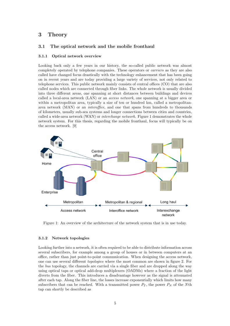
Looking back only a few years in our history, the so-called public network was almostcompletely operated by telephone companies. These operators or carriers as they are alsocalled have changed focus drastically with the technology enhancement that has been goingon in recent years and are today providing a large variety of services, not only related totelephone services. This public network mainly consists of central offices (CO) that are alsocalled nodes which are connected through fiber links. The whole network is usually dividedinto three different areas, one spanning at short distances between buildings and devicescalled a local-area network (LAN) or an access network, one spanning at a bigger area orwithin a metropolitan area, typically a size of ten or hundred km, called a metropolitan-area network (MAN) or an interoffice, and one that spans from hundreds to thousandsof kilometers, usually sub-sea systems and longer connections between cities and countries,called a wide-area network (WAN) or interchange network. Figure 1 demonstrates the wholenetwork system. For this thesis, regarding the mobile fronthaul, focus will typically be onthe access network. [9]

Figure 1: An overview of the architecture of the network system that is in use today.

3.1.2 Network topologies

Looking further into a network, it is often required to be able to distribute information acrossseveral subscribers, for example among a group of houses or in between computers at anoffice, rather than just point-to-point communication. When designing the access network,one can use several different topologies where the most common are shown in figure 2. Forthe bus topology, the channels are carried via a single fiber and are dropped along the wayusing optical taps or optical add-drop multiplexers (OADMs) where a fraction of the lightdiverts from the fiber. This introduces a disadvantage however as the signal is attenuatedafter each tap. Along the fiber line, the losses increase exponentially which limits how manysubscribers that can be reached. With a transmitted power PT , the power PN of the N thtap can shortly be described as

5

PN = PTC[(1− δ)(1− C)]N−1 (1)

where C is the fraction of the power transmitted further to each node and δ is the insertionloss at each tap. For this example, C and δ are assumed to be the same for each tap.

For the hub topology, the distribution of channels is acquired at a certain location called”hub” which is done in the electrical domain before transmitting the signal further overfiber. This topology is typically used in bigger cities connecting several nodes and officestogether. Both the bus and hub topologies are usually used for larger networks such as inMANs. A disadvantage with them however is that if there is a fiber outage in the link, alarge number of the nodes may get affected. [23]

(a) Bus. (b) Hub.

(c) Ring. (d) Star.

Figure 2: Depicting networks with four different topologies.[23]

For shorter distances and smaller networks, typically within a LAN, ring and star topologiesare more common. For the ring topology, several nodes are connected via point-to-point fiberin a closed route, where each node receives and transmits data further which then can workas a repeater. [10] For a star topology, all nodes are connected to a central hub via point-to-point fiber. This center hub can be either a passive or active unit. For an active hub, theoptical signals are first converted to electrical signals before being processed, while for thepassive hub, the distribution amongst the nodes is done optically via couplers. As for thecase with the bus topology, the number of subscribers connected to the star will be limitedby the distribution losses. Assuming an ideal N ×N coupler, each node will receive a powerof PT /N from a signal with transmitted power PT . By introducing insertion losses δ to thenodes, the power received at each node, PN , can be written as

PN = (PT /N)(1− δ)log2N (2)

6

Here, the log2N comes from the interconnections between the 3 dB couplers that are neededto achieve an N ×N coupler. [23]

3.1.3 The new mobile fronthaul architecture

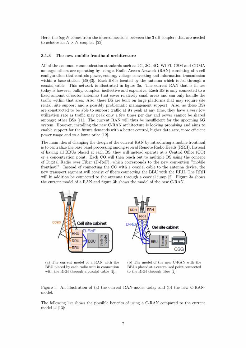
All of the common communication standards such as 2G, 3G, 4G, Wi-Fi, GSM and CDMAamongst others are operating by using a Radio Access Network (RAN) consisting of a cellconfiguration that controls power, cooling, voltage converting and information transmissionwithin a base station (BS)[3]. Each BS is located by the antenna which is fed through acoaxial cable. This network is illustrated in figure 3a. The current RAN that is in usetoday is however bulky, complex, ineffective and expensive. Each BS is only connected to afixed amount of sector antennas that cover relatively small areas and can only handle thetraffic within that area. Also, these BS are built on large platforms that may require siterental, site support and a possibly problematic management support. Also, as these BSsare constructed to be able to support traffic at its peak at any time, they have a very lowutilization rate as traffic may peak only a few times per day and power cannot be sharedamongst other BSs [11]. The current RAN will thus be insufficient for the upcoming 5Gsystem. However, installing the new C-RAN architecture is looking promising and aims toenable support for the future demands with a better control, higher data rate, more efficientpower usage and to a lower price [12].

The main idea of changing the design of the current RAN by introducing a mobile fronthaulis to centralize the base band processing among several Remote Radio Heads (RRH). Insteadof having all BBUs placed at each BS, they will instead operate at a Central Office (CO)or a concentration point. Each CO will then reach out to multiple BS using the conceptof Digital Radio over Fiber (D-RoF), which corresponds to the new convention ”mobilefronthaul”. Instead of connecting the CO with a coaxial cable to the antenna device, thenew transport segment will consist of fibers connecting the BBU with the RRH. The RRHwill in addition be connected to the antenna through a coaxial jump [2]. Figure 3a showsthe current model of a RAN and figure 3b shows the model of the new C-RAN.

(a) The current model of a RAN with theBBU placed by each radio unit in connectionwith the RRH through a coaxial cable [2].

(b) The model of the new C-RAN with theBBUs placed at a centralized point connectedto the RRH through fiber [2].

Figure 3: An illustration of (a) the current RAN-model today and (b) the new C-RAN-model.

The following list shows the possible benefits of using a C-RAN compared to the currentmodel [4][13]:

7

• Replacing the coaxial cable with fiber reduces the power consumption by firstly elimi-nating the electrical losses in the coaxial cable but also by moving the power amplifierfrom the base station to the RRH.

• With a DAS, it is possible to drive several antenna systems from one central office.The transmitted power can thus be adjusted to spread to the antennas covering theareas with the highest traffic at that moment, reducing power that is wasted on areasthat might not be in use at that specific moment. This will thus improve the efficiency.An example of a DAS is shown in figure 4.

• The replacing of the coaxial cable with fiber is also a matter of data transmissionspeed. A fiber can carry an optical signal of the order Tb/s while the coaxial cableonly can support a transmission speed of an order of Mb/s, resulting in a 106-orderdifference.

• With a centralized system, the C-RAN will be much easier to install and maintain asthe BBUs for several antenna systems will be located at a central office compared tohaving the BBUs at each antenna. Thus, both time and money can be saved in theinstallation and maintenance process.

Figure 4: Using the concept of DAS, multiple antenna systems can be controlled from onebase band unit [4].

The challenge with the C-RAN architecture however is, as mentioned in the introduction,that the mux and demuxers, i.e. the filters, will be placed next to the RRH close to theantenna, exposing them to possibly rougher climates, where mostly thermal changes mayaffect the performance of the rather sensitive filters. Thus, it is of interest to characterizethese filters.

Moreover, the idea of the new architecture is to place the antennas a maximum of 20 kmaway from the CO. With such a short distance, the signals are much unlikely to suffer fromdB-penalties from dispersion, polarization losses or optical signal to noise ratio (OSNR)-related penalties, which thus needn’t be neither considered in the study nor discussed forfuture work.

3.2 Transmission characteristics of filters

In the following section, a couple of relevant filter characteristics or parameters are definedand explained. Throughout the study and the report, the signals are described in frequencies,f rather than wavelengths, λ. Also, to simplify calculations, the power levels are measured

8

in a 10-based logarithmic scale with the unit dB. When analyzing optical systems, it is alsoof interest to study the power level related to 1 mW of power, where the unit then is denoteddBm. Adding to this, a system that sends information separated at different frequencies iscalled a Wavelength Division Multiplexing (WDM) system, compared to the Time DivisionMultiplexing (TDM) system.

3.2.1 Insertion loss and isolation

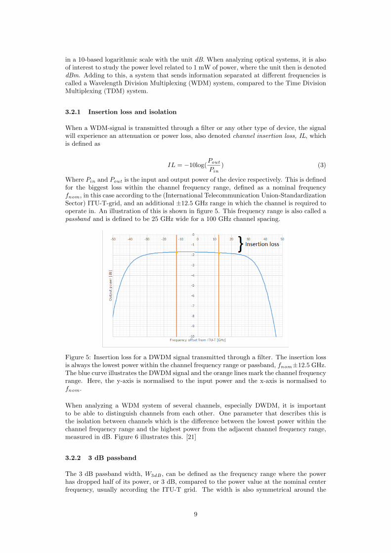
When a WDM-signal is transmitted through a filter or any other type of device, the signalwill experience an attenuation or power loss, also denoted channel insertion loss, IL, whichis defined as

IL = −10log(PoutPin

) (3)

Where Pin and Pout is the input and output power of the device respectively. This is definedfor the biggest loss within the channel frequency range, defined as a nominal frequencyfnom, in this case according to the (International Telecommunication Union-StandardizationSector) ITU-T-grid, and an additional ±12.5 GHz range in which the channel is required tooperate in. An illustration of this is shown in figure 5. This frequency range is also called apassband and is defined to be 25 GHz wide for a 100 GHz channel spacing.

Figure 5: Insertion loss for a DWDM signal transmitted through a filter. The insertion lossis always the lowest power within the channel frequency range or passband, fnom±12.5 GHz.The blue curve illustrates the DWDM signal and the orange lines mark the channel frequencyrange. Here, the y-axis is normalised to the input power and the x-axis is normalised tofnom.

When analyzing a WDM system of several channels, especially DWDM, it is importantto be able to distinguish channels from each other. One parameter that describes this isthe isolation between channels which is the difference between the lowest power within thechannel frequency range and the highest power from the adjacent channel frequency range,measured in dB. Figure 6 illustrates this. [21]

3.2.2 3 dB passband

The 3 dB passband width, W3dB , can be defined as the frequency range where the powerhas dropped half of its power, or 3 dB, compared to the power value at the nominal centerfrequency, usually according the ITU-T grid. The width is also symmetrical around the

9

Figure 6: Adjacent isolation for a DWDM signal transmitted through a filter. The bluecurve illustrates the DWDM signal, the orange lines mark the channel frequency range andthe grey line marks the outer frequency limit for an adjacent channel that is 100 GHz apartin this case.

center frequency, i.e. the 3 dB passband is whithin the range of fnom ±W3dB/2. Hence,the power may have dropped 3 dB on one side of the passband but only 2 dB on the otherside when comparing the same drift from the center wavelength. An illustration of this isshown in figure 7. [21]

Figure 7: The 3 dB passband of a channel shown according to the definition. [21]

3.2.3 Center wavelength drift

The center wavelength for a channel can be defined as the average of all wavelengths withina 3 dB drop from the peak value of a channel. [17] The difference between the center wave-length of the channel and the channel wavelength defined from the ITU-T grid is called thecenter wavelength offset. When the temperature of the filter changes, the center wavelengthof the filter channels may drift leading to a change in the offset from the ITU-T grid. Thedrift is measured in GHz for this thesis but is usually also measured in nm.

3.2.4 Crosstalk

When multiplexing or demultiplexing a DWDM signal using a filter, the goal is to transmitas much power as possible from the wanted channel and attenuate all others. However, dueto imperfections in the filter, the filter may leak power from the adjacent and non-adjacentchannels which then interferes with the primary channel. This is called crosstalk and can

10

be defined as the ratio of the total power of the primary signal to the total power of theinterfering signals, computed as

εX =

∫ f0−f0 X(f)df∫ f0−f0 S(f)df

(4)

where X(f) is the interfering signal, S(f) is the primary signal and f0 is a frequency rangethat covers the bandwidth of the signal.[22] Crosstalk is a big concern for DWDM systems asa higher crosstalk may increase the BER and thus limits the transmission distance. Figure 8shows a simulation made in VPI of the transmission power of 16 channels through an AWGfilter. As can be seen, the filter is far from perfect in isolating adjacent channels which allinterfere with each other.

Figure 8: 16 AWG channels with a channel spacing of 100 GHz, simulated in VPI.

3.3 Receivers

3.3.1 Bit-Error Rate

When an optical signal is received at the receiver end, the signal is sampled at a decisiontime tD with a certain sampling frequency. One way to measure the performance of anoptical receiver is to look at the bit-error rate (BER) which is defined as the ratio of everywrong bit over every received bit, or as the probability to detect an incorrect bit. A commoncriterion for optical receivers is a BER below 10−9, i.e maximum one bit per billion may beincorrect. Since the probability for a 0 and a 1 to occur are equal, the BER can be definedusing both the probabilities of detecting a 1 when a 0 was received and detecting a 0 whena 1 was received as [23]

BER =1

2

[P (0/1) + P (1/0)

](5)

These probabilities will depend on a probability function p(I) of the sampled values I. I1represents the average signal level of a 1-bit and I0 represents the average signal level of a 0-bit. As the incoming signal will be affected by several kinds of noise, which can be describedwith Gaussian statistics, the signal will fluctuate around I1 and I0, each with correspondingvariances σ1 and σ0. Using these values, one can define the probabilities P (0/1) and P (1/0)as [23]

11

P (0/1) =1

σ1√

2π

∫ ID

−∞exp

(− (I − I1)2

2σ21

)dI =

1

2erfc

((I1 − ID)

σ1√

2

)(6)

P (1/0) =1

σ0√

2π

∫ ∞ID

exp

(− (I − I0)2

2σ20

)dI =

1

2erfc

((ID − I0)

σ0√

2

)(7)

which are illustrated in figure 9. Here, erfc is the complementary error function which isdefined as [27]

erfc(x) =2√π

∫ ∞x

exp(−y2)dy (8)

Figure 9: The fluctuations at the I1 and I0 levels can be described with two Gaussiandistributed functions with corresponding variances σ1 and σ0 from which P (0/1) and P (1/0)can be calculated.

Once calculating the BER based on measurements, one must make sure to measure enoughbits to ensure that the BER values are within some level of confidence. This can be donewith the following formula for the confidence level CL

CL = 1− e−N×BER ×E∑k=0

(N ×BERS)k

k!(9)

where N is the number of transmitted bits, E is the number of incorrect bits and BERS isthe specified or required BER. Theoretically, CL will always be less than 100 % since onecannot measure for an infinite length of time, thus one must choose a reasonable confidencelevel. Many industries consider at least 95 % as a valid level, which has been decided to beused for this study as well. [24]

3.3.2 FEC

One way of improving the performance of an optical transmission system is to employ aforward error correction (FEC), which allows a system to tolerate a higher BER before thereceiver reliability is reduced too much. [14] A FEC method that is very common is theReed-Solomon (RS) FEC. It is based on adding redundant bits to the data words that areto be transmitted. Consider an amount of data with n codewords which are n symbolslong. The data can be divided into block codes that are defined by k number of symbolsof real data and an additional r numbers of redundant symbols (also called parity symbols)corresponding to the redundant data. By knowing the position and values of these symbols,

12

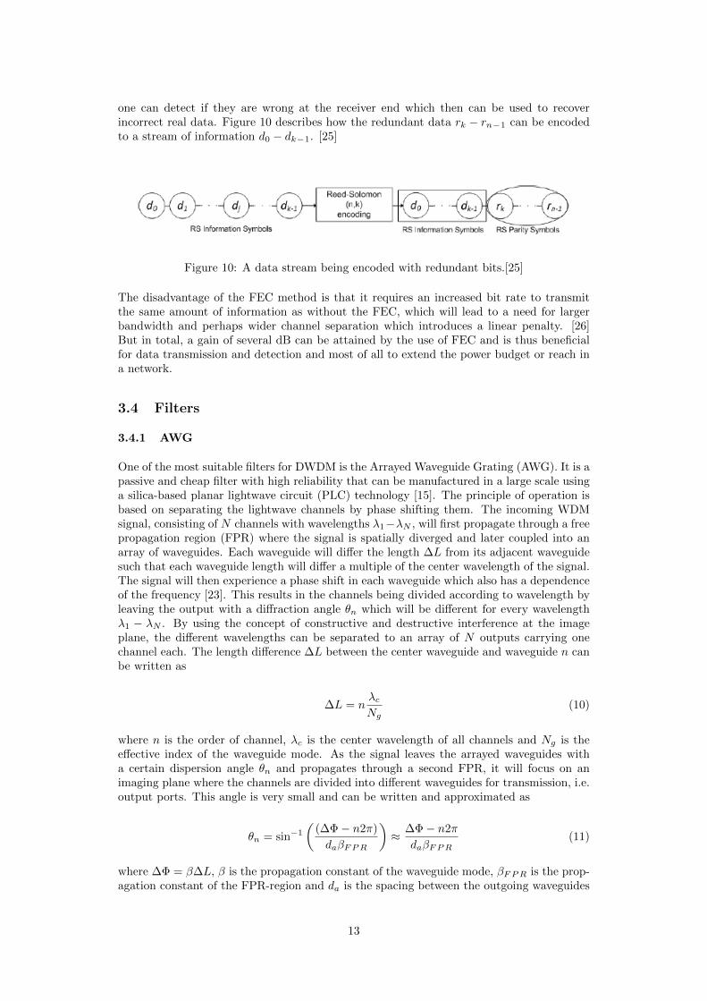
one can detect if they are wrong at the receiver end which then can be used to recoverincorrect real data. Figure 10 describes how the redundant data rk − rn−1 can be encodedto a stream of information d0 − dk−1. [25]

Figure 10: A data stream being encoded with redundant bits.[25]

The disadvantage of the FEC method is that it requires an increased bit rate to transmitthe same amount of information as without the FEC, which will lead to a need for largerbandwidth and perhaps wider channel separation which introduces a linear penalty. [26]But in total, a gain of several dB can be attained by the use of FEC and is thus beneficialfor data transmission and detection and most of all to extend the power budget or reach ina network.

3.4 Filters

3.4.1 AWG

One of the most suitable filters for DWDM is the Arrayed Waveguide Grating (AWG). It is apassive and cheap filter with high reliability that can be manufactured in a large scale usinga silica-based planar lightwave circuit (PLC) technology [15]. The principle of operation isbased on separating the lightwave channels by phase shifting them. The incoming WDMsignal, consisting of N channels with wavelengths λ1−λN , will first propagate through a freepropagation region (FPR) where the signal is spatially diverged and later coupled into anarray of waveguides. Each waveguide will differ the length ∆L from its adjacent waveguidesuch that each waveguide length will differ a multiple of the center wavelength of the signal.The signal will then experience a phase shift in each waveguide which also has a dependenceof the frequency [23]. This results in the channels being divided according to wavelength byleaving the output with a diffraction angle θn which will be different for every wavelengthλ1 − λN . By using the concept of constructive and destructive interference at the imageplane, the different wavelengths can be separated to an array of N outputs carrying onechannel each. The length difference ∆L between the center waveguide and waveguide n canbe written as

∆L = nλcNg

(10)

where n is the order of channel, λc is the center wavelength of all channels and Ng is theeffective index of the waveguide mode. As the signal leaves the arrayed waveguides witha certain dispersion angle θn and propagates through a second FPR, it will focus on animaging plane where the channels are divided into different waveguides for transmission, i.e.output ports. This angle is very small and can be written and approximated as

θn = sin−1(

(∆Φ− n2π)

daβF PR

)≈ ∆Φ− n2π

daβF PR(11)

where ∆Φ = β∆L, β is the propagation constant of the waveguide mode, βF PR is the prop-agation constant of the FPR-region and da is the spacing between the outgoing waveguides

13

as shown in figure 12 [16]. A benefit of the AWG is that it is reciprocal and may thus beused both for multiplexing and demultiplexing.

Figure 11: A schematic of an AWG [23].

Figure 12: A schematic of how each signal is focused at a single output port [16].

The aim with the filter is to achieve a transfer function with a low insertion loss, sharp skirtsand small sidelobes, preferably close to a rectangular pass band function or a Super-Gaussianof high order to reduce crosstalk and thus the BER [28]. This is even more important forDWDM applications where the channel spacing usually is 100 GHz or lower which meansthat the channels are even more vulnerable to crosstalk. Assuming that the incoming signals

have a Gaussian distribution exp(−y2

2σ2 ) and that the total number of waveguides are 2P + 1,where P is a positive integer, then the transfer function of the filter from the input waveguideto the central output waveguide can be expressed as

Hq(f) =

P∑n=−P

Cnexp(j2πtnf − jκynyqof) (12)

where yqo is the distance from the central output waveguide to the output waveguide n.

Since the AWG-filter is highly dependent on the phase shifts generated by the length dif-ference ∆L, it follows that the AWG is very sensitive to changes in temperature as it mayimplement small expansions or contractions in the material which may cause the channelsto focus at the wrong output port, leading to higher losses, more crosstalk and in generala worse filter performance. To avoid this, one can either keep the temperature constant byinstalling it in a controlled environment, or one can use an athermal AWG that compensatesfor the material changes caused by thermal changes. This is generally done in two ways,either by applying a material with a negative dn

dT in the optical path, such as resin-filledgrooves,[19] or by mechanically moving the input fiber with a metal board that will expandor contract with temperature so that it compensates for the focus shift [20]. An illustrationof this is shown in figures 13 and 14.

14

Figure 13: A shift in focus on the output ports can be compensated by mechanically movingthe output lens according to the change in temperature.[18]

Without a thermal compensation, a silica-based AWG can have a center wavelength drift ofapproximately 10 pm/◦C which can be severe for long transmissions at a very high or lowtemperature. But with a first order thermal compensation, the center wavelength drift canbe reduced to only a couple of pm/◦C. A case with and without thermal compensation areshown in figure 14.

Figure 14: An overview of a conventional AWG where focus point output has a larger driftat higher and lower temperatures compared to an athermal AWG where a shift of the metalboard compensates for the focus drift.

3.4.2 TFF

Figure 15: The principle of a Fabry-Perot filter consisting of two mirrors that separatelightwaves of different frequencies. [9].

The thin film filter (TFF) is a resonant multicavity filter that uses the same principle asa Fabry-Perot filter. The cavity consists of two highly reflective mirrors or films, parallelto each other, separated a distance l. This allows some wavelengths of light to propagatethrough the mirrors while some are reflected which is shown in figure 15. The light that willtravel multiples of half their wavelength through the length of the cavity will always havethe same phase when leaving the right mirror and are thus called resonant wavelengths [9].

15

The power transmitted through the filter can be expressed with the following function

T (f) =(1− A

1−R )2

1 + ( 2√R

1−R sin(2πfτ))2(13)

where A is the absorption loss and R is the reflectivity for each mirror and τ is the propa-gation delay across one cavity length. Figure 16 shows the transfer function for a filter withA = 0 and R = 0.75,R = 0.90 and R = 0.99. One can see that a higher reflectivity leads tosharper filter functions with higher isolation.

Figure 16: A transfer function for a TFF with A = 0 and R = 0.75, R = 0.90 and R = 0.99[9].

What also can be noted is that the transfer function is periodic in f and will peak for everyfτ = k/2 for a positive integer k and may thus coincide with an adjacent channel. Thespectral space between two peaks is called the free spectral range (FSR). To avoid crosstalkas much as possible, two different channels must be separated by at least one Full WidthHalf Maximum (FWHM) of the signals in addition to a spectral range distance of k×FSRfor a positive integer k.

One of the benefits with a Fabry-Perot filter is that it can be tuned simply by changingthe cavity length or the refractive index in the cavity. The filtered frequency is selected tosatisfy

f0τ = k/2 (14)

for a positive integer k. And with

τ =ln

c(15)

where n is the refractive index, l is the distance between the mirrors and c is the speed oflight. The filtering frequency f0 can be changed by either changing l or n.

When designing a TFF, several Fabry-Perot filters are put in cascade where each filtercorresponds to one channel. The effect however is that for every filter that the signal passesthrough, the filter function will change, which can be seen in figure 18. After every filter,the transfer function becomes sharper at the skirts. The TFF is reciprocal like the AWGfilter, meaning that it can be used both to multiplex and demultiplex channels. Figure 16shows an overview of a TFF filter with eight Fabry-Perot filters in cascade, resulting in amultiplexing/demultiplexing of eight different channels with wavelengths λ1 − λ8.

3.4.3 Interleaver

With an increasing demand for data capacity, a more effective usage of the bandwidthsare needed to enable more channels to be packed within the DWDM-band. As many filter

16

Figure 17: An overview of a TFF filter with eight Fabry-Perot filters in cascade [9].

Figure 18: Transfer functions for one, two and three Fabry-Perot filters in cascade [9].

technologies are limited to a specified channel spacing, an optical interleaver can be used tocut down the channel spacings even more. [29] The purpose of an optical interleaver is toseparate or combine incoming channels of a DWDM signal with a periodic spacing betweenchannels. The most basic interleaver, denoted 1:2, divides the incoming signal into oddand even channels. An example could be a system with channels that are 50 GHz apart,which then are divided into two systems where the signals are 100 GHz apart. Other typicalinterleavers are 1:4 or 1:8 which separate every fourth or eighth channel respectively, but fora general case, there are also 1:N interleavers, separating every N:th channel [30]. Figure 19shows an example of a 1:2 and a 1:4 interleaver.

Figure 19: A 1:2 and 1:4 interleaver. Here, λe= even λ, λo= odd λ and λa−d= four differentchannel spacings [30].

The interleaver consists in most cases of an optical interferometer, such as a Michelson inter-

17

ferometer, where the output is a result from the interference created by the interferometerwhich thus will be periodic with frequency. The period of the interleaver is decided by thelength difference of the two arms and the distance between the two mirrors where the signalis reflected. Figure 20 shows an example of an interleaver with two Gires-Tournois etalons(GTEs) as mirrors [29].

Figure 20: A schematic of a GTE interleaver [29].

The intensity of the output can be written as

I =1

2

[1 + cos

(2π

cν2∆L+ (ϕ2 − ϕ1)

)](16)

where ∆L is the difference between L1 and L2, ν is the optical frequency and ϕ1 and ϕ2 arethe phase shifts between the two mirrors where the difference can be written

ϕ2 − ϕ1 = 2 tan−1[

1 +√R2

1−√R2

tan(φ)

]− 2 tan−1

[1 +√R1

1−√R2

tan(φ)

](17)

where R1 and R2 are the reflectivities of the front mirrors on the first and second arm andφ is the phase shift due to the distance travelled within the GTEs.

In measurement tests, interleavers have been able to separate channels with spacings of100, 50, 25 and 12.5 GHz for DWDM. The free spectral range (FSR) of the filter functiondecides the period of the interleaver [31] and can be seen in figure 21. In order to alignthe interleavers with the DWDM signals, to avoid a mismatch between signals and filtersleading to walkoff losses, it is of high importance that both the signals and the interleaverfollow the specifications set by the International Telecommunication Union (ITU). Apartfrom this possible alignment error, there can also be offset errors, or drifts, that may arisedue to thermal changes [30], just as for the passive AWG or TFF.

Figure 21: A transfer function of an interleaver with a 50 GHz cycle [30].

18

4 Methods and measurements

The following section describes how the lab equipment was set up, how the data was recordedand handled and how the results were found from these. More information about the specificfilters that were used are also presented here, such as how the interior of the filter looks likeand how the filter channels are positioned. This section only considers the specification ofthe filters while the background theory and functionality is described in section 3.4 Filters.

4.1 Filters

4.1.1 TFF

When a signal enters the TFF from the line, the signal will first go through an 8-skip-0filter which simply is just a bandpass filter that is selected to cover all the eight channelsfor this specific filter. In typical systems with 40 channels, the signals will go through fiveTFFs which are in cascade, each with an individual 8-skip-0 filter to filter out the relevantbandpass to fit the output ports of each filter. Here, the filter is designed to have fouradd/drop pairs, i.e four pairs of channels, one as a transceiver port and one as a receiverport, but since each port is reciprocal, it can be used as eight bidirectional channels. Forthis filter, the names of the ports are connected to the center frequency of that port, e.g.port number 926 has a center frequency of 192.6 THz. The ports are 100 GHz separated infrequency, which is typical for a DWDM filter.

Figure 22: A schematic of the TFF with an 8-skip-0 filter and the following four add/droppairs.

4.1.2 AWG

Unlike the TFF, the AWG can mux and demux 40 channels at once from the line. This AWGis also athermal, meaning that when temperature changes, a metal board will compensatefor the focus shift that appears and align the channel signal to the right port. Also the portsof the AWG are separated 100 GHz from each other.

4.1.3 Interleaver

This interleaver has one input to demultiplex channels of 50 GHz spacing into two outputsof 100 GHz spacings, one odd output and one even. The Interleaver is reciprocal and canthus also be used to multiplex two channels into one. In this thesis, the even output hasbeen used since that matches channel spacing of the TFF and AWG.

19

Figure 23: A schematic of the 40 channel athermal AWG filter with a 100 GHz channelspacing, here with a monitor (tap coupler) attached to the line, but that won’t be used inthis thesis. Channel 1 corresponds to the 191.9 THz channel, channel 40 corresponds to the195.8 THz channel, TX means ”transceived” and RX means ”received”.

4.2 Lab setups

The following sections describe the procedure of the measurements, how the lab equipmentwas used and set up and how the measurements were performed. To start with, all mea-surements were put in two different categories: one for measurement of filter parameterssuch as passband, isolation, insertion loss, center wavelength drift and crosstalk, and onefor measurement of the BER. These two tests were performed at different occasions for eachfilter. The following list describes the measurements in more detail.

Filter characterization:

• Measure insertion loss and isolation [dBm] with respect to temperature [◦C] using alightwave multimeter (Agilent 8163A Lightwave Multimeter). The measurement willbe done on a couple of chosen channels using an adjustable transceiver.

• Measure the 3 dB passband [GHz], with respect to temperature [◦C], from the filters’transfer functions using an optical spectrum analyzer (AQ6370D Yokagawa). Theinserted signal will be from an amplified spontaneous emission (ASE) source.

• Measure center wavelength drift [GHz] with respect to temperature [◦C] using anoptical spectrum analyzer (AQ6370D Yokagawa). The inserted signal will be from anamplified spontaneous emission (ASE) source.

• Measure crosstalk [dB] over temperature [◦C] using an optical spectrum analyzer(AQ6370D Yokagawa) and compare it with isolation measurements done with thelightwave multimeter.

BER measurements:

• Measure bit error rate (BER) with respect to temperature [◦C] and with respect toadjacent channels using a BER-tester (Anritsu MP1800A Signal Quality Analyzer).

Before the measurements were initiated, the method had to be decided regarding whatfilter channels to collect data from, what temperatures and how the measurements shouldbe performed in detail. Firstly, it was decided to analyze only three different channelsfor every filter setup, two at the edges of the filter channels and one in the middle. Thisresulted in choosing channels 919, 922 and 926 for the TFF and channels 1, 20 and 40 for

20

the AWG. Table 1 shows the specified frequencies and wavelengths for each channel. Thetemperatures at which to collect data were chosen to -40, -20, 0, 25, 50, 70 and 85 ◦C, sincethe standardized I-temp is defined as -40-85 ◦C. The filters have been located in a Votschtemperature chamber (VT3 7060) and the temperature has been measured both with theVotsch and a thermometer (Fluke 50D Thermometer) with probes located in the middle ofthe Votsch chamber and close to the filter module.

Filter Channel Frequency[THz]

Wavelength[nm]

TFFch 919 1.9190 1562.23ch 922 1.9220 1559.79ch 926 1.9260 1556.55

AWGch 1 1.9580 1531.12ch 20 1.9390 1546.12ch 40 1.9190 1562.23

Table 1: The specified frequency and wavelength for each channel that has been used in themeasurements.

4.2.1 Filter characterization

The following section describes the procedures of each measurement for the filter character-ization in the same order as above. Here, the input power is a signal from the ASE-sourcewhich basically amplifies white noise to a power level of approximately 15-20 dBm and coversall frequencies relevant to the measurements done on the filters. This is shown in figure 24where the ASE-source has been measured with the Yokogawa, covering the whole ASE-span.

Figure 24: A graph showing the power of the ASE-light measured with the Yokogawa. Thefilters used in this study all operate within the same frequency span as the passband of theASE-light.

The following list describes the procedures that were done for each measurement in the filtercharacterization.

• Insertion loss. To achieve the insertion loss for every filter at every temperature, allthe measured power data was used to plot graphs of the filter functions. Each channel,or filter function, was plotted against the frequency offset from the ITU-T definition(see table 1). Using this offset, the insertion loss could be found by taking the lowestpower within the ±12.5 GHz offset.

To double check that the insertion loss had been calculated correctly, it was alsomeasured with the Agilent 8163A Lightwave Multimeter. This was done both for theTFF and the AWG filter for all channels using an optically tunable transceiver laser

21

as an input signal. The signals were measured both with and without the filters for allchannels. The difference between the input signal and the output signal of the filteris equal to the insertion loss of the filter. The results are provided in table 6. Themeasurement was done at a temperature of 25 ◦C.

• Isolation. To find the adjacent isolation for each channel, the highest power withinthe bandwidth of the adjacent channels according to the ITU-T grid were taken. Thiswas done for both the right and left channel, were the isolation was noted as the worstof these two.

• Filter function. When using the Yokogawa to measure the filters’ transfer functions,the measurement procedure always started with collecting data from the ASE-source,sweeping across all relevant frequencies. This was done daily as a start for every mea-surement. Each channel was then collected separately to the Yokogawa and was sweptacross a relevant frequency band. Since the ASE-source is not perfectly distributedover the frequency-band within the TFF and AWG filters, and not at 0 dBm power,the correct transfer function had to be calculated by taking the difference betweenthe ASE-source and the output signal from the chosen channel, which was done withthe Yokogawa. This resulted in a plot of the power in logarithmic scale of the filterfunction against frequency in linear scale. An example of this measurement can beseen in figure 48. Apart from collecting data from the filter function, the Yokogawa’sfilter functions were also used to calculate center wavelength, peak value, 3 dB pass-band width, 10 dB passband width, ripple and also crosstalk to the left and right ofthe signal. This data was however only used to compare and confirm that my owncalculations seemed correct.

• 3 dB passband. When calculating the 3 dB passband for each channel, the power atthe center wavelength calculated by the Yokogawa was used. Then the power level wasnoted 3 dB below the center power level on both sides of the center wavelength. Theminimum wavelength at where the power had dropped 3 dB, called f3dB was used todefine the 3 dB passband as the frequency range fcenter ± fcenter−f3dB

2 where fcenteris defined according to the ITU-T grid [21].

• Crosstalk. For the calculation of the crosstalk, the method consisted of finding theworst case adjacent and non-adjacent isolations of all channels that were measured.This was done by finding all maximum power levels within the adjacent and non-adjacent channels, i.e. within fchannel±12.5 GHz, where fchannel is defined accordingto the ITU-T grid, converting them to a linear scale, add them up and then convertthem back to logarithmic power. The result is the total crosstalk or the total isolationof all channels combined.

The measurements were done in the lab at Infinera with their own equipment. Table 2 showsa measurement matrix of all the measurements that were done in the filter characterizationand figure 25 shows a sketch of the lab setup and what equipment was used where the redline shows the transmission line of the signal from start to end. Moreover, the interface ofthe Yokogawa is shown in figure 26 with an example of a measurement done on the AWGfilter.

22

AWG TFF Interleaver+AWG

Interleaver+TFF

Insertion lossIsolation3 dB passbandCenter wavelength driftCrosstalk

Table 2: Depicting an overview matrix for all measurements that were done in the filtercharacterization.

Figure 25: The lab setup for the filter characterization. In the figure, the numbers correspondto: 1. ASE-source 2. Votsch chamber 3. Votsch thermometer 4. Interleaver 5. AWG orTFF 6. The Fluke thermometer 7. The Yokogawa Optical Spectrum Analyzer.

Figure 26: An overview of the Yokogawa interface for a measurement on the AWG filter. Inthe picture, the purple curve represents the light from the ASE-source, the yellow curve isthe transfer function of the filter and the green curve is the difference between the transferfunction and the ASE-source, i.e a normalization of the filter function relative the ASE-source. The pink curves in the middle of the AWG passband are the 10G signals transmittedat a frequency of 192.0 THz.

23

4.2.2 BER measurements

The following section describes the measurement procedure for the BER measurements.

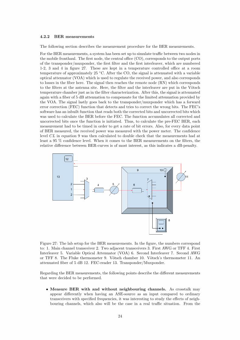
For the BER measurements, a system has been set up to simulate traffic between two nodes inthe mobile fronthaul. The first node, the central office (CO), corresponds to the output portsof the transponder/muxponder, the first filter and the first interleaver, which are numbered1-2, 3 and 4 in figure 27. These are kept in a temperature controlled office at a roomtemperature of approximately 25 ◦C. After the CO, the signal is attenuated with a variableoptical attenuator (VOA) which is used to regulate the received power, and also correspondsto losses in the fiber here. The signal then reaches the remote node (RN) which correspondsto the filters at the antenna site. Here, the filter and the interleaver are put in the Votschtemperature chamber just as in the filter characterization. After this, the signal is attenuatedagain with a fiber of 5 dB attenuation to compensate for the limited attenuation provided bythe VOA. The signal lastly goes back to the transponder/muxponder which has a forwarderror correction (FEC) function that detects and tries to correct the wrong bits. The FEC’ssoftware has an inbuilt function that reads both the corrected bits and uncorrected bits whichwas used to calculate the BER before the FEC. The function accumulates all corrected anduncorrected bits once the function is initiated. Thus, to calculate the pre-FEC BER, eachmeasurement had to be timed in order to get a rate of bit errors. Also, for every data pointof BER measured, the received power was measured with the power meter. The confidencelevel CL in equation 9 was then calculated to double check that the measurements had atleast a 95 % confidence level. When it comes to the BER measurements on the filters, therelative difference between BER-curves is of most interest, as this indicates a dB-penalty.

Figure 27: The lab setup for the BER measurements. In the figure, the numbers correspondto: 1. Main channel transceiver 2. Two adjacent transceivers 3. First AWG or TFF 4. FirstInterleaver 5. Variable Optical Attenuator (VOA) 6. Second Interleaver 7. Second AWGor TFF 8. The Fluke thermometer 9. Votsch chamber 10. Votsch’s thermometer 11. Anattenuated fiber of 5 dB 12. FEC-reader 13. Transponder/Muxponder.

Regarding the BER measurements, the following points describe the different measurementsthat were decided to be performed.

• Measure BER with and without neighbouring channels. As crosstalk mayappear differently when having an ASE-source as an input compared to ordinarytransceivers with specified frequencies, it was interesting to study the effects of neigh-bouring channels, which also will be the case in a real traffic situation. From the

24

25 ◦C 85 ◦CCO RN With

neigh-bours

Withoutneigh-bours

Withneigh-bours

Withoutneigh-bours

Without AWG2 AWG3Interleaver AWG2 TFFWith AWG2 AWG3Interleaver AWG2 TFF

Table 3: Depicting an overview matrix for all BER measurements that were performed. Thefilters have been put in two nodes, one in a central office (CO) and one in the remote node(RN) i.e close to the antenna for the realistic case.

results in the filter characterization, especially figures 41-42, it was decided togetherwith the supervisors that only traffic on the adjacent channels would suffice. Theadjacent channels are both numbered 2 in figure 27.

• Signal formats. The card in the transponder/muxponder scrambles a signal by itselfif no signal is received at the receiver. When calculating BER, a scrambled signal isto prefer as random bits are harder to repair compared to defined patterns.

• New AWG filters. As the BER measurements include two filters at two nodes,instead of just measuring on one filter as in the filter characterization, it was decidedto analyze two new AWG filters, which have the same article number, are manufacturedin the same way and have the same functionality. Since it’s a node to node connection,it was relevant to connect an AWG-A with an AWG-B. It may be a disadvantage tonot use the same filter as in the filter characterization, but as it was interesting to addanother AWG, which doesn’t differ very much, it was considered to be a safe change.No measurements have been done on the new AWGs apart from the test measurementsdone by the manufacturers. Thus, a comparison between the filter characteristics forthese three filters could be made. To avoid confusion, these new AWGs have beenlabeled ”AWG2” and ”AWG3”. When it comes to the TFF, the same filter has beenused and only once in the BER measurements. Thus, the TFF is only labeled as”TFF”. See table 3 for more details.

• With and without interleavers. Similar as in the filter characterization, the nodesare also to be connected both with and without interleavers. As for the case withthe AWG, an additional interleaver had to be used. This interleaver is also the sametype as the one used in the filter characterization and shouldn’t necessarily cause anyapparent affect on the results. Measurement data to compare with can be seen infigure 59.

• Temperatures. For the BER measurements, it was decided to mainly focus on thetemperatures that were worst in the filter characterization, which in general was forwarmer temperatures. Thus, the measurements were done at 25 and 85 ◦C.

To add credibility to the study and to make sure that the test results are valid, the followingextra measurements were made.

• Measure crosstalk from the adjacent channels. To easier understand how theBER-curves are affected by more traffic on the line, the power at the channel wasmeasured for six different traffic situations using a power meter. These are representedin table 4 where 1 and 0 correspond to the laser being on and off respectively. Theadjacent channels were chosen to be 100 GHz away from the main channel, i.e. oneoutput port away at the TFF and AWG filters. All three channels for all filters weretransmitted at 10 Gb/s at a temperature of 25 ◦C using the tunable transmitter. From

25

the results in figure 41 and 42 one can see that the adjacent channels contribute themost to the crosstalk compared to the non-adjacent channels. Thus, it was decidedthat only two adjacent channels, one at each side of the channel, would suffice for thismeasurement.

Adjacent channel left 0 1 0 1 0 1Main channel 1 1 0 0 0 0Adjacent channel right 0 1 0 0 1 1Measured power [dB]

Table 4: An overview of six different traffic situations with or without adjacent channelsand the main channel. Here 1 and 0 correspond to the laser being on and off respectively.

• Measuring BER with a BERT. To make sure that the FEC-reader software pro-gram could be used to calculate BER, the method was compared to another mea-surement that included a bit error rate tester (BERT). The BERT used for this wasthe Anritsu MP1800A Signal Quality Analyzer. This BERT generates a certain pseu-dorandom binary sequence (PRBS) that has a certain cycle of random bits whilewithout the BERT, the signal is just scrambled randomly. The PRBS patterns thatwere considered were PRBS7 and PRBS31, i.e. cycles with 27−1 and 231−1 differentbit-combinations per cycle. The setup for the BER-measurement with the BERT isvery similar to the setup in figure 27 but without the adjacent channels and with theBERT instead of the transponder/muxponder. In order to achieve the correct wave-length on the transceiver, two additional transceivers and a HEX-light card had to beused. These transceivers have a specified maximum bit rate of 10.3 Gb/s however, butcould be used anyway to support 11.1 Gb/s.

• Measuring the transceiver. To add further credibility to the measurements, thetransceiver alone was measured for BER without any filter. The signal was sent at a11.1 Gb/s rate with both a PRBS31 and PRBS7 pattern.

4.2.3 Temperature control

Since each of the four filter technologies had to be measured at -40, -20, 0, 25, 50, 70 and85 ◦C, i.e at seven different temperatures, it implied that at least 7× 4 = 28 measurementshad to be done. To avoid as much sources of error as possible, it was important to makesure that each measurement would be as similar as possible in the procedure. Therefore, afirst temperature test was made on the TFF filter, heating it from room temperature to 60◦C and measuring the temperature both with the Votsch thermometer, but also with twoprobes from the Fluke thermometer, one located inside the filter module and one located inthe middle of the Votsch chamber. By every third minute, the temperatures were sampled,which are summarized in table 5 below.

As can be seen from table 5 and figure 28 by comparing the temperatures, it’s easy toconclude that the heating of the filter is lagging behind the heating of the chamber but alsothe temperatures of the Fluke thermometer and the Votsch may differ by several degrees.After 12 minutes, there is a temperature difference of approximately 12 ◦C between thefilter and the chamber temperature measured by the Fluke thermometer. As temperatureincreases, the material of the filter will expand, thus a temperature difference between theinterior and the exterior of the filter may lead to tensions in the material which can beharmful. Since the filters are very sensitive to length contractions and extractions, it wasdecided to change the temperature using a ramp function with a lower time derivativecompared to using a jump function that was used in this test. A ramp with a 2 ◦C/minderivative was used. Also, to save time, the cover of the TFF module was always removed toallow the filter to change temperature quicker. The AWG was however delivered without acover. To make sure that the filters reached the right temperature, the time between starting

26

Time [min] Temperatureinside thechamber[◦C]

Temperatureinside thefilter[◦C]

Votsch tem-perature [◦C]

0 22.8 22.9 22.13 27.7 24.8 34.56 35.6 27.0 44.79 42.2 30.5 54.312 47.5 35.0 58.715 50.6 39.3 59.618 52.7 43.0 60.221 54.3 46.1 60.124 55.3 48.7 60.127 56.3 50.9 60.030 56.9 52.9 60.033 57.4 54.1 60.036 57.7 55.2 60.039 57.9 56.0 60.042 58.2 56.8 60.045 58.5 57.5 60.048 58.6 57.8 60.051 58.7 58.1 60.054 58.8 58.3 60.057 59.0 58.6 60.060 59.0 58.8 60.0

Table 5: Temperatures inside the chamber, inside the filter and of the Votsch plotted againsttime.

Figure 28: A plot of the data provided in table 5.

the ramp and the measurements were always at least one hour long. Both the temperaturefrom the Fluke and the Votsch were noted at each measurement. However, the temperaturesfrom the Fluke and the Votsch always differed by a few degrees, probably due to a poorcalibration of the Fluke, so the measurements were done only when both the temperaturesfrom the Fluke and the Votsch had saturated.

27

4.3 Simulations

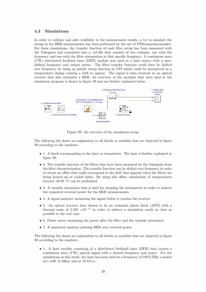
In order to validate and add credibility to the measurement results, a try to simulate thesetups in the BER measurements has been performed by the use of VPItransmissionmaker.For these simulations, the transfer function of each filter setup has been measured withthe Yokogawa and translated into a .txt-file that consists of two columns, one with thefrequency and one with the filter attenuation at that specific frequency. A continuous wave(CW) distributed feedback laser (DFB) module was used as a laser source with a user-defined frequency and output power. The filter transfer function could then be driftedover frequency by using an inbuilt sweep function in VPI which could be interpreted as atemperature change causing a drift to appear. The signal is then received at an opticalreceiver that also estimates a BER. An overview of the modules that were used in thesimulation program is shown in figure 29 and are further explained below.

Figure 29: An overview of the simulation setup.

The following list shows an explanation to all blocks or modules that are depicted in figure29 according to the numbers.

• 1. A block corresponding to the laser or transmitter. The laser is further explained infigure 30.

• 2. The transfer function of the filters that have been measured by the Yokogawa fromthe filter characterization. The transfer function can be shifted over frequency in orderto attain an offset that could correspond to the drift that appears when the filters arebeing heated up or cooled down. By using this offset, simulations of temperaturesbeyond -40-85 ◦C can be performed.

• 3. A variable attenuator that is used for stepping the attenuation in order to achievethe requested received power for the BER measurements.

• 4. A signal analyzer measuring the signal before it reaches the receiver.

• 5. An optical receiver, here chosen to be an avalanche photo diode (APD) with athermal noise of 2.535 ×10−11 in order to achieve a simulation result as close aspossible to the real case.

• 6. Power meter measuring the power after the filter and the variable attenuator.

• 7. A numerical analyzer plotting BER over received power.

The following list shows an explanation to all blocks or modules that are depicted in figure30 according to the numbers.

• 1. A laser module consisting of a distributed feedback laser (DFB) that creates acontinuous wave (CW) optical signal with a desired frequency and power. For thesimulations in this study, the laser has been used at a frequency of 192.0 THz, a powerof 1 mW (0 dBm) and at 10 Gb/s.

28

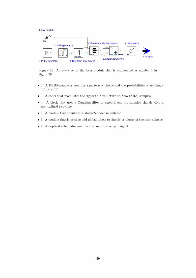
Figure 30: An overview of the laser module that is represented as number 1 infigure 29.

• 2. A PRBS-generator creating a pattern of choice and the probabilities of sending a”0” or a ”1”.

• 3. A coder that modulates the signal to Non Return to Zero (NRZ) samples.

• 4. A block that uses a Gaussian filter to smooth out the sampled signals with auser-defined rise-time.

• 5. A module that simulates a Mach-Zehnder modulator

• 6. A module that is used to add global labels to signals or blocks of the user’s choice.

• 7. An optical attenuator used to attenuate the output signal.

29

5 Results and analysis

5.1 Filter characterization

The following sections present the results from the filter characterization. Each section offigures is followed by an analysis and explanation to the results. Shortly, the filter charac-terization concerns the characteristics of each filter setup regarding insertion loss, isolation,filter transfer functions, 3 dB passband, center wavelength drift and crosstalk that have beendescribed above in section 3 Theory and 4 Methods and measurements.

5.1.1 Insertion loss and isolation

The following section addresses the measurements and calculations on insertion loss andisolation. The results provided in table 6 can be compared to the calculated results measuredby the Yokogawa presented in figures 31 and 32.

Filter andchannel num-ber

Inputpower fromtransceiver[dBm]

Measuredpowerthrough filter[dBm]

Calculatedinsertion loss[dB]

TFF 919 0.20 -1.86 2.06TFF 922 0.14 -1.71 1.85TFF 926 0.08 -2.29 2.38AWG 1 0.61 -3.67 4.28AWG 20 0.56 -3.47 4.03AWG 40 0.33 -4.49 4.82

Table 6: Table depicting the input power of the transceiver, received power to the powermeter with the filters and the resulting insertion loss. The measurement was done at atemperature of 25 ◦C.

Figure 31: Insertion loss plotted overtemperature for the TFF for all threechannels.

Figure 32: Insertion loss plotted overtemperature for the AWG for all threechannels.

30

On pages 31-34, the adjacent isolation has been plotted for each filter technology. The threesignal curves in every graph labeled (a) are taken from the lowest (i.e. worst) isolations inthe graphs denoted (b)-(d). Also, the figure at the bottom of each page shows an example ofwhere the isolation data has been found for three different temperatures from the adjacentchannels. For the cases where the interleaver is connected, the worst adjacent isolation hasbeen gathered from a channel passband 50 GHz away from the main channel instead of 100GHz.

(a) Adjacent isolation for each channel. (b) Left and right adjacent isolation for channel919.

(c) Left and right adjacent isolation for channel922.

(d) Left and right adjacent isolation for channel929.

Figure 33: Adjacent isolation plotted over temperature for the TFF.

Figure 34: TFF channel 919 at -40, 25and 85 ◦C.

31




Figure 35: Adjacent isolation plotted over temperature for the Interleaver+TFF.

Figure 36: Interleaver+TFF channel 1 at-40, 25 and 85 ◦C.

32




Figure 37: Adjacent isolation plotted over temperature for the AWG.

Figure 38: AWG channel 1 at -40, 25 and85 ◦C.

33




Figure 39: Adjacent isolation plotted over temperature for the Interleaver+AWG.

Figure 40: Interleaver+AWG channel 1at -40, 25 and 85 ◦C.

34

For the following graphs on page 36 and 37, the maximum power within a 25 GHz frequencyspan has been plotted for all adjacent and non-adjacent channels, which are represented bythe datapoints. The graphs have been normalised to the output power of the main channel.This has been done for three different temperatures of -40, 25 and 85 ◦C.

35

(a) Non-adjacent isolation for TFF, channel919.

(b) Non-adjacent isolation for Inter-leaver+TFF, channel 919.

(c) Non-adjacent isolation for TFF, channel922.

(d) Non-adjacent isolation for Inter-leaver+TFF, channel 922.

(e) Non-adjacent isolation for TFF, channel926.

(f) Non-adjacent isolation for Interleaver+TFF,channel 926.

Figure 41: Non-adjacent isolation plotted for each channel for the TFF to the left andInterleaver+TFF to the right at -40, 25 and 85 ◦C.

36

(a) Non-adjacent isolation for AWG, channel 1. (b) Non-adjacent isolation for Inter-leaver+AWG, channel 1.

(c) Non-adjacent isolation for AWG, channel20.

(d) Non-adjacent isolation for Inter-leaver+AWG, channel 20.

(e) Non-adjacent isolation for AWG, channel40.

(f) Non-adjacent isolation for Inter-leaver+AWG, channel 40.

Figure 42: Non-adjacent isolation plotted for each channel for the AWG to the left andInterleaver+AWG to the right at -40, 25 and 85 ◦C.

37

Firstly, by studying figure 31 for both the TFF and the Interleaver+TFF, one can see thatall channels follow the same pattern over temperature, but channel 919 and 922 have almostthe same values compared to channel 926. A similar pattern can be seen in figure 32 wherechannel 1 and 20 behave alike while channel 40 has a slightly higher insertion loss. Thiscould be due to the structures of the filters. For the TFF, channel 919 is the first outputchannel and is thus only filtered through a Fabry-Perot filter once, while 922 is the fourthin the order and 926 is the very last output. For every output that the signal passes, thebandpass filter function will be narrower.

What also can be concluded is that the insertion loss is worst for low temperatures when theinterleaver is connected to either of the AWG or TFF but seems to be more or less unaffectedat higher temperatures as the worst total insertion loss difference is approximately 0.4 dBacross the whole temperature span.

Looking at the adjacent isolation for the TFF in figure 33a one can see that the isolationis stable for all channels, where the biggest difference is 1.9 dB over the whole temperaturerange. However, there is a huge difference in isolation between the channels, where channel919 is the best with an isolation of approximately 60 dB, while channel 926 and 922 have anisolation of approximately 45 dB and 40 dB respectively. The reason for this big differencecan be understood by looking at figure 44. It can be seen that channels 922 and 926 haveasymmetric transfer functions and have a flatter roll-off at the filter function’s right skirtcompared to channel 919, which contributes to a smaller worst case adjacent isolation.

From figure 37a of the AWG’s adjacent isolation on the other hand, a different patternappears where the isolation seems to be best at temperatures of -20, 50 and 70 ◦C. Thiscan be explained with figure 52b where the center wavelength drift is lowest at -20, 50 and70 ◦C and worse at the other temperatures. By comparing figure 31 with figure 32, figure33a with figure 37a and figure 44 with figure 45 one may conclude that the TFF has both alower insertion loss and a higher isolation compared to the AWG in general.

By analyzing figure 35a and 39a one can see that the poor isolation from the interleavercomes in place and is in most effect at the higher temperatures. An interesting note regardingthe TFF is that when the interleaver is connected, the adjacent isolation is worst for channel926 while it’s worst for channel 922 when the interleaver is not connected. For this case, theisolation is measured 50 GHz away from the main channel instead of 100 GHz.

Moreover, an interesting note is to compare the drifts that appear for the transfer functionsof the filters by looking at figures 34, 36, 38 and 40. Here, one can clearly see how a highertemperature shifts the TFF transfer functions from the left to the right, while for the casewith the AWG, both the transfer functions for -40 and 85 ◦C lie to the right of the transferfunction for 25 ◦C which is explained by the athermalization of the AWG filter done by themetal board.

38

5.1.2 Crosstalk

The following figures show the results from the crosstalk calculations. Here, the crosstalklevels are equal to the sum of the highest power within all adjacent and non-adjacent chan-nels. When the interleaver is connected, the data has been collected with a channel spacingof 50 GHz and with the interleaver connected, the data has been collected with a channelspacing of 100 GHz.

(a) Total crosstalk plotted against temperaturefor the TFF.

(b) Total crosstalk plotted against temperaturefor the AWG.

(c) Total crosstalk plotted against temperaturefor the Interleaver+TFF.

(d) Total crosstalk plotted against temperaturefor the Interleaver+AWG.

Figure 43: Total crosstalk plotted against temperature for all filters.

What can be seen from the total crosstalk figures is that the crosstalk looks very similar tothe adjacent isolation in figures 33a, 35a, 37a and 39a. The plots approximately follow thesame shape, but the crosstalk level is roughly 3 dB lower than the adjacent isolation, whichalso is expected in general. For the AWG as an example, the adjacent channel isolation isspecified for 25 dB while the total crosstalk is specified to be 22 dB. What this implies isthat most of the crosstalk comes from the adjacent channels, but also approximately 3 dB ofthe crosstalk is generated from non-adjacent channels. Thus, this section analyses a widerspan of channels while the isolation section only goes into the neighbouring channels.

By studying figure 43c, one can see that channels 922 and 926 have a higher crosstalk astemperature rises compared to channel 919 which can be explained with the asymmetricaltransfer function of channels 922 and 926. As a drift appears with higher temperature,the isolation will increase at the right skirts of the filter transfer function which is shownclearly for channels 922 and 926, but not for 926 as that one has a sharper filter skirt.When it comes to the AWG in figure 43b, most of the crosstalk comes from the adjacentchannel here aswell, which can be seen in the drift and reversed drift of the filter function

39

as temperature changes. An interesting phenomena is found in figure 43d where the totalcrosstalk seems to be relatively stable over temperature until 85 ◦C where the crosstalkfor all channels is increased by approximately 2 dB. For this scenario, as the interleaver isconnected, the crosstalk is measured at a spacing of only 50 GHz, which could lead to theisolation of the adjacent channel to be poor here together with the drift that appears at thehigh temperature which is analyzed further below.

5.1.3 Filter functions

The following figures on page 41 show examples of what the filter transfer functions look like.Figures 44 and 45 show the transfer functions of the TFF and AWG for the three differentchannels that were measured for each filter, also with the channel passband and where theadjacent channels are located in the spectrum. Figures 46 and 47 show the filter functions ofall the channels that were measured with the interleaver attached to the line. The blue linealso shows the transfer function of the interleaver. In figures 48 and 49, a chosen channelhas been plotted both with the interleaver connected and disconnected together with thetransfer function of the interleaver, to easier see how the interleaver affects the transferfunctions of the signals. All figures have been normalised to the input power on the y-axisand to a chosen channel frequency on the x-axis.

40

Figure 44: TFF channels 919, 922 and926 at 25 ◦C.

Figure 45: AWG channels 1, 20 and 40 at25 ◦C.

Figure 46: The channels plotted for boththe TFF and the Interleaver over fre-quency at 25 ◦C.

Figure 47: The channels plotted for boththe AWG and the Interleaver over fre-quency at 25 ◦C.

Figure 48: The channels plotted for theInterleaver, Int+TFF and TFF over fre-quency at 25 ◦C.

Figure 49: The channels plotted for theInterleaver, Int+AWG and AWG over fre-quency at 25 ◦C.

41

5.1.4 3 dB Passband

The following figures present the 3 dB measurements done for each filter setup for eachchannel. Figure 51 also presents the average passband over temperature for the interleaver.

(a) 3 dB passband for the TFF plotted overtemperature.

(b) 3 dB passband for the AWG plotted overtemperature.

(c) 3 dB passband for the Interleaver+TFFplotted over temperature.

(d) 3 dB passband for the Interleaver+AWGplotted over temperature.

Figure 50: 3 dB passband plotted for all four filter setups.

Figure 51: 3 dB passband for the Inter-leaver plotted over temperature.

42

When studying the 3 dB-passband for the three TFF-channels in figure 50a, one may besurprised at the different derivatives of the passband for the different channels compared tothe AWG in figure 50b where the passband remains relatively constant over temperature.A similar behaviour can be seen in figure 50c where the interleaver also is connected, buthere, the passband has been narrowed down to the passband of the interleaver, which canbe seen in figure 51. The same goes for the Interleaver+AWG in figure 50d. Though thebandwidth has decreased from approximately 80 GHz to 50 GHz, the number of channelshave doubled, now with a 50 GHz spacing instead of 100 GHz. Furthermore, for the casewith the TFF being connected to the interleaver in figure 50c, the decrease for channel 919can be explained with figure 52a. Channel 919 has first of all an offset from the ITU-Tgrid and secondly, as the interleaver and TFF drift in opposite ways, the passband will benarrowed down for higher temperatures. In the same situation for the AWG, in figure 50d,the passband seems to alternate over temperature, which also has an explanation related tothe drift seen in figure 52b. As the AWG drifts back and forth, while the interleaver driftslinearly, the passband will experience an alternating width.

The vendor of the TFF explained that the reason for the odd behaviour in figure 50a wasjust random. We however suggest that there could be an explanation that has to do witheach Fabry-Perot mirror inside the TFF. Our guess is that as temperature changes, alsothe reflectivity, R could change, leading to some frequencies being more reflected and somebeing less reflected. Thus, if the reflectivity increases for the first mirror, the transceivedsignal will be decreased and more power will go on to the next pair of mirrors where thesame thing happens. Eventually, the last output signal will have more power than before,which possibly could be proportional to the 3 dB passband.

43

5.1.5 Center wavelength drift

(a) Center wavelength drift for the TFF plot-ted over temperature.

(b) Center wavelength drift for the AWGplotted over temperature.

(c) Center wavelength drift for the Inter-leaver+TFF plotted over temperature.

(d) Center wavelength drift for the Inter-leaver+AWG plotted over temperature.

Figure 52: Center wavelength drift for all filter setups over temperature.

Figure 53: Average frequency drift for 11channel periods of the Interleaver.

44

As for the center wavelength drift as a function of temperature, all TFF channels seem tofollow the same shape of the drift by looking at figure 52a. The channels do not behavealike however. Channel 919, 922 and 926 have a total drift of 4.02, 2.28 and 5.27 GHzrespectively and channel 919 has a larger offset from the ITU-T grid compared to 922 and926. An overview of the drifts can also be detected in figure 34 and 38 where channel 919for the TFF and channel 1 for the AWG have been plotted for -40, 25 and 85 ◦C.

The U-shape of the frequency drift for the AWG in figure 52b can be explained with theathermalization design of the AWG filter. The filter’s inbuilt metal board will move accord-ing to the temperature change which compensates for the expansion or contraction of theAWG waveguides due to temperature changes. What can be concluded also is that as thefilter expands at higher temperatures, the offset between channels varies more compared tocolder temperatures which is a clear consequence of the expansion of the AWG waveguides.

When it comes to the interleaver connected to the TFF and the AWG however, the channelsare now drifting with the interleaver which can be seen by comparing figure 52c and 52dwith figure 53. The only difference is that the interleaver drifts with a maximum totalvalue of 4.17 GHz while the Interleaver+AWG and Interleaver+TFF have a maximum totaldrift of 4.07 and 4.08 GHz respectively. In addition to this, it seems that the drift is morecritical at high temperatures compared to low temperatures, as the biggest drift appearsat 85 ◦C. Moreover, looking at figure 52a, the TFF drifts in the opposite way compared tothe interleaver, but as the passband of the interleaver is smaller compared to the TFF, thecenter wavelength will simply follow the center of the interleaver.

45

5.2 BER measurements

The following section presents results and analysis from the BER measurements. It startswith the control measurements before going into the pure BER-results. Shortly, this cate-gory concerns how the BER looks like for the different filter setups and how it varies overtemperature and with or without adjacent channels.

5.2.1 Crosstalk from adjacent channels

In the following subsection, an analysis has been made regarding the measurements oncrosstalk from adjacent channels and how that may affect the BER for the different filtersetups. For these measurements, the two VOAs were used to adjust the output power byadding or subtracting attenuation to the traffic to compensate for the four different insertionlosses for the four different filter setups. As presented in tables 7-10, channel 920 was chosenas the main channel with channels 919 and 921 as adjacent channels, which are 100 GHzapart from 920. An important note here for the case with the interleavers connected isthat although the channels are supposed to be transmitted 50 GHz apart, they have stillbeen measured with channels transmitted 100 GHz apart. This can be explained with theinterleaver having both an odd and even output and the filters are also either odd or even.Thus, in a real situation, there would be a possibility to transmit 80 channels at a 50 GHzspacing, but the ports at the filters will still be 100 GHz away by using one 40 channel oddfilter and one 40 channel even filter. In the tables, 1 and 0 correspond to the laser being onand off respectively.

AWG2 and AWG3

a b c d e fch 919 (left) 0 1 0 1 0 1ch 920 (main) 1 1 0 0 0 0ch 921 (right) 0 1 0 0 1 1Measured power [dB] -16.0 -16.0 -64.9 -55.4 -55.0 -52.5

Table 7: An overview of six different traffic situations with or without adjacent channelsand the main channel for the case with AWG2 and AWG3.

AWG2, AWG3 and Interleavers


Table 8: An overview of six different traffic situations with or without adjacent channelsand the main channel for the case with AWG2, AWG3 and Interleavers.

When analyzing the numbers provided in tables 7-10, the relative difference between eachsituation is of most importance rather than the values themselves. What is common for allfour filter setups is that the power for traffic situation a and b is practically the same. Theadditional power from the adjacent channels in situation b is at least attenuated approxi-mately 30 dB, i.e. 1000 times lower, compared to the main channel, which is too small todetect on the power meter. By comparing the numbers in situation c, d, e and f, one can findmore to discuss. Starting from situation c, with no channels turned on, one can immediatelysee that the TFF attenuates the crosstalk better than the AWG does by comparing situation

46

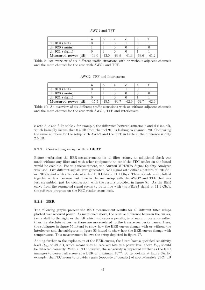
AWG2 and TFF


Table 9: An overview of six different traffic situations with or without adjacent channelsand the main channel for the case with AWG2 and TFF.

AWG2, TFF and Interleavers


Table 10: An overview of six different traffic situations with or without adjacent channelsand the main channel for the case with AWG2, TFF and Interleavers.

c with d, e and f. In table 7 for example, the difference between situation c and d is 8.4 dB,which basically means that 8.4 dB from channel 919 is leaking to channel 920. Comparingthe same numbers for the setup with AWG2 and the TFF in table 9, the difference is only2.6 dB.

5.2.2 Controlling setup with a BERT

Before performing the BER-measuerements on all filter setups, an additional check wasmade without any filter and with other equipments to see if the FEC-reader on the boardwould be credible. For this measurement, the Anritsu MP1800A Signal Quality Analyzerwas used. Five different signals were generated, each signal with either a pattern of PRBS31or PRBS7 and with a bit rate of either 10.3 Gb/s or 11.1 Gb/s. These signals were plottedtogether with a measurement done in the real setup with the AWG2 and TFF that wasjust scrambled, just for comparison, with the results provided in figure 54. As the BERcurve from the scrambled signal seems to be in line with the PRBS7 signal at 11.1 Gb/s,the software program on the FEC-reader seems legit.

5.2.3 BER

The following graphs present the BER measurement results for all different filter setupsplotted over received power. As mentioned above, the relative difference between the curves,i.e. a shift to the right or the left which indicates a penalty, is of more importance ratherthan the absolute values, as those are more related to the transceiver performance. Here,the subfigures in figure 55 intend to show how the BER curves change with or without theinterleaver and the subfigures in figure 56 intend to show how the BER curves change withtemperature. This measurement follows the setup depicted in figure 27.

Adding further to the explanation of the BER-curves, the filters have a specified sensitivitylevel Prec of -24 dB, which means that all received bits at a power level above Prec shouldbe detected correctly. With a FEC however, the sensitivity is improved further as the FECmanages to correct all errors at a BER of maximum 10−4. So by looking at figure 55a forexample, the FEC seems to provide a gain (opposite of penalty) of approximately 31-24 dB

47

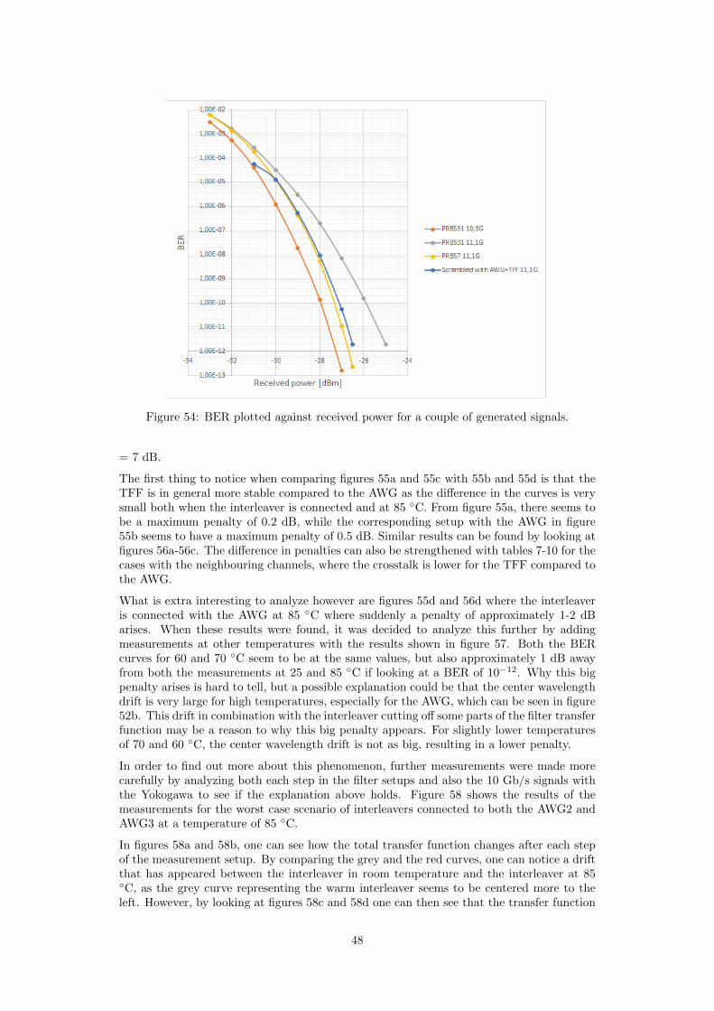
Figure 54: BER plotted against received power for a couple of generated signals.

= 7 dB.

The first thing to notice when comparing figures 55a and 55c with 55b and 55d is that theTFF is in general more stable compared to the AWG as the difference in the curves is verysmall both when the interleaver is connected and at 85 ◦C. From figure 55a, there seems tobe a maximum penalty of 0.2 dB, while the corresponding setup with the AWG in figure55b seems to have a maximum penalty of 0.5 dB. Similar results can be found by looking atfigures 56a-56c. The difference in penalties can also be strengthened with tables 7-10 for thecases with the neighbouring channels, where the crosstalk is lower for the TFF compared tothe AWG.

What is extra interesting to analyze however are figures 55d and 56d where the interleaveris connected with the AWG at 85 ◦C where suddenly a penalty of approximately 1-2 dBarises. When these results were found, it was decided to analyze this further by addingmeasurements at other temperatures with the results shown in figure 57. Both the BERcurves for 60 and 70 ◦C seem to be at the same values, but also approximately 1 dB awayfrom both the measurements at 25 and 85 ◦C if looking at a BER of 10−12. Why this bigpenalty arises is hard to tell, but a possible explanation could be that the center wavelengthdrift is very large for high temperatures, especially for the AWG, which can be seen in figure52b. This drift in combination with the interleaver cutting off some parts of the filter transferfunction may be a reason to why this big penalty appears. For slightly lower temperaturesof 70 and 60 ◦C, the center wavelength drift is not as big, resulting in a lower penalty.

In order to find out more about this phenomenon, further measurements were made morecarefully by analyzing both each step in the filter setups and also the 10 Gb/s signals withthe Yokogawa to see if the explanation above holds. Figure 58 shows the results of themeasurements for the worst case scenario of interleavers connected to both the AWG2 andAWG3 at a temperature of 85 ◦C.

In figures 58a and 58b, one can see how the total transfer function changes after each stepof the measurement setup. By comparing the grey and the red curves, one can notice a driftthat has appeared between the interleaver in room temperature and the interleaver at 85◦C, as the grey curve representing the warm interleaver seems to be centered more to theleft. However, by looking at figures 58c and 58d one can then see that the transfer function

48

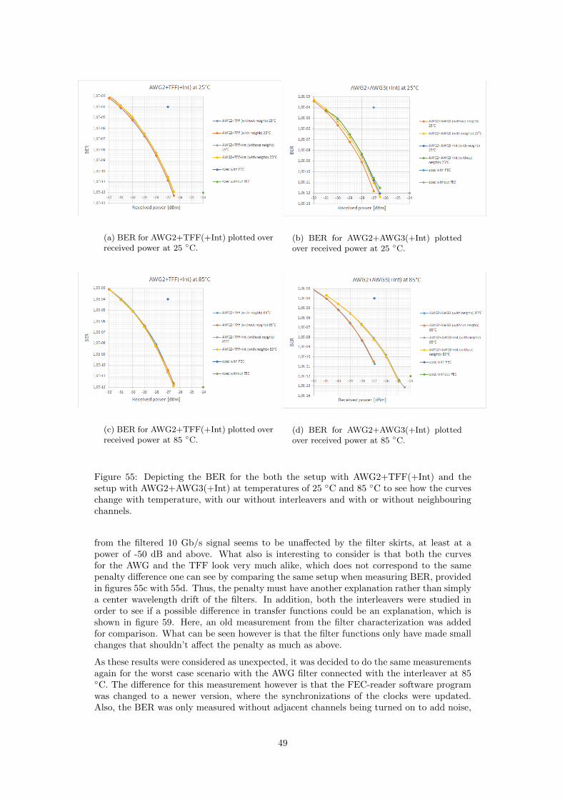
(a) BER for AWG2+TFF(+Int) plotted overreceived power at 25 ◦C.

(b) BER for AWG2+AWG3(+Int) plottedover received power at 25 ◦C.

(c) BER for AWG2+TFF(+Int) plotted overreceived power at 85 ◦C.

(d) BER for AWG2+AWG3(+Int) plottedover received power at 85 ◦C.

Figure 55: Depicting the BER for the both the setup with AWG2+TFF(+Int) and thesetup with AWG2+AWG3(+Int) at temperatures of 25 ◦C and 85 ◦C to see how the curveschange with temperature, with our without interleavers and with or without neighbouringchannels.

from the filtered 10 Gb/s signal seems to be unaffected by the filter skirts, at least at apower of -50 dB and above. What also is interesting to consider is that both the curvesfor the AWG and the TFF look very much alike, which does not correspond to the samepenalty difference one can see by comparing the same setup when measuring BER, providedin figures 55c with 55d. Thus, the penalty must have another explanation rather than simplya center wavelength drift of the filters. In addition, both the interleavers were studied inorder to see if a possible difference in transfer functions could be an explanation, which isshown in figure 59. Here, an old measurement from the filter characterization was addedfor comparison. What can be seen however is that the filter functions only have made smallchanges that shouldn’t affect the penalty as much as above.

As these results were considered as unexpected, it was decided to do the same measurementsagain for the worst case scenario with the AWG filter connected with the interleaver at 85◦C. The difference for this measurement however is that the FEC-reader software programwas changed to a newer version, where the synchronizations of the clocks were updated.Also, the BER was only measured without adjacent channels being turned on to add noise,

49

(a) BER for AWG2+TFF plotted over re-ceived power at 25 ◦C and 85 ◦C.

(b) BER for AWG2+AWG3 plotted over re-ceived power at 25 ◦C and 85 ◦C.

(c) BER for AWG2+TFF+Int plotted overreceived power at 25 ◦C and 85 ◦C.

(d) BER for AWG2+AWG3+Int plotted overreceived power at 25 ◦C and 85 ◦C.

Figure 56: Depicting the BER for both the setup with AWG2+TFF(+Int) and the setupwith AWG2+AWG3(+Int) at temperatures of 25 ◦C and 85 ◦C to see how the curves changewith temperature, with our without interleavers and with or without neighbouring channels.

as this seemed to have very low effect for the previous cases. As can be seen in the resultsin figure 60, the penalty is now only approximately 0.4-0.5 dB, which is lower compared tothe results in figures 55d and 56d. Considering that these results arose after an update onthe FEC-reader, one may consider these new results to be more credible than the previousones. However, the credibility of the whole method might be questioned as the results havebeen varying from time to time and without any clear reason. This is discussed further insection 6.2 Measurement errors.

50

Figure 57: BER for AWG2+AWG3+Int plotted over received power at 25, 60, 70and 85 ◦C.

51

(a) Each filter function for every step throughthe setup, here with a TFF as the final fil-ter. Each function is normalized to 0 dBm.

(b) Each filter function for every stepthrough the setup, here with a AWG as thefinal filter. Each function is normalized to 0dBm.

(c) The final filter function for the case withthe TFF together with the transfer functionsof the 10 Gb/s signal, both filtered and un-filtered with a normalization to 0 dBm.

(d) The final filter function for the case withthe AWG together with the transfer func-tions of the 10 Gb/s signal, both filtered andunfiltered with a normalization to 0 dBm.

Figure 58: Four graphs depicting the change of the filter function after each filter and alsowith the actual 10 Gb/s signal transmitted at 192.0 THz.

52

Figure 59: The transfer functions for both interleavers at different temperatures.

Figure 60: New BER values for AWG2+AWG3+Int plotted over received powerat 25 ◦C and 85 ◦C. Here only without adjacent channels for the case of 85 ◦C.

53

5.2.4 Simulation results

The following section contains simulation results done according to the description in section4.3 Simulations.

The very first thing to do was to calibrate the simulations in order to find a setup as closeas possible to the real measurements. This was mainly done by changing the responsivityof the APD receiver which corresponds to the electrical photocurrent per unit optical powerthat is induced in the photodiode. This was done plotting measurement results from thesetup with the AWG2 and TFF together with a set of simulations with different values ofthe responsivity. The results of this is seen in figure 61 and as can be seen, a responsivityof 1 seems to match the measurement results the best.

Figure 61: Depicting the same measurement results as in 56a with additional sim-ulation results plotted with different receiver responsivity settings of 0.8, 0.9, 0.95and 1.

In figure 62a, a simulation has been done using the transfer function for the setup withAWG2 and AWG3 interconnected with two interleavers at 85 ◦C, which was the worst casescenario. In order to achieve BER-values at a relevant level, the variable attenuator, or blocknumber 3 in figure 29, was chosen to step from 12 dB to 21 dB with one dB-steps. Thesimulation was then run while doing discrete sweeping of the filter transfer function withsteps of 4 GHz, which correspond to the different curves in figure 62a. The more the filteris drifted, the more attenuated the received power will be, which explains why the curvesstart and end at different received power values in the graph. As can be seen for both figure62a and 62b, the BER is unaffected at drifts of 1-12 GHz, but at a drift of 16 GHz, theBER-curves starts deviating and a penalty arises. At 20 GHz, the penalty is even higher.

In addition, a simulation was made with the worst case scenario for the AWGs connectedwith interleavers for both 25 and 85 ◦C in order to see if a BER penalty would arise asmeasured. The result is seen in figure 64, where the plots for both the temperatures are ontop of each other, indicating no penalty. What can be seen however is that the 85 ◦C-curve ismore attenuated compared to the 25 ◦C-curve as the corresponding data points are shifted.This must not necessarily affect the BER however.

54

(a) Results from simulating BER forAWG2+AWG3+Int plotted over receivedpower for drifts of 0, 4, 8, 12, 16 and 20 GHz.

(b) Results from simulating BER forAWG2+TFF+Int plotted over receivedpower for drifts of 0, 4, 8, 12, 16 and 20 GHz.

Figure 62: Simulation results with drift iterations added for the worst case scenario for boththe AWG and TFF.

(a) Measurement and simulation results ofBER for AWG2+AWG3+Int plotted over re-ceived power

(b) Measurement and simulation results ofBER for AWG2+TFF+Int plotted over re-ceived power.

Figure 63: Measurement and simulation results of TFF for AWG2+AWG3+Int plotted overreceived power.

55

Figure 64: Depicting the same measurement results as in 56d with additionalsimulation results with the same setup but for 25 and 85 ◦C.

56

6 Discussion

For the discussion, I have foremost decided to evaluate the different filter setups with a tech-nical analysis based on the results provided above, both from measurements and simulations.But in order to put the results into a bigger context related to a realistic scenario, I havealso added a discussion on power budget. Furthermore, I have addressed some issues thatarose throughout the thesis and how they may have affected the credibility of the results.As a final discussion, I have also considered the ethical aspects related to the study, and howthe results can be implemented for a more realistic case based on more than just technicalaspects. This discussion will then work as a base for the conclusions in the next section.

6.1 Technical aspects

In the following section, I have decided to evaluate and compare each filter based on theresults in the filter characterization and BER measurements, discuss these and try to putthem into a bigger context. In order to make it easier for the reader to follow the discussion,the evaluations and comparisons are presented in the list below for each filter parameterthat has been measured in accordance to the results above.

• Insertion loss. When comparing the results of the filters for the insertion loss infigures 31 and 32, one can clearly see a comparison between filters and also overtemperature. Here, the TFF seems to have approximately 2-2.5 dB lower insertionloss than the AWG, while with the interleaver connected, another 1 dB in insertionloss is added. Looking at the temperature-dependence, the insertion loss is in generalstable for all filter setups, differing a maximum of 0.5 dB over the whole temperaturerange, where cold temperature seems to be most severe at least by looking at figure32. All measurements are however within the specified values provided by the vendors.This insertion loss can be considered as a pure penalty, which affects reach in theend. Thus, the TFF can be considered to have approximately 2-2.5 dB lower penaltycompared to the AWG.

When it comes to application areas, for a simple mobile fronthaul scenario with fibers ofa maximum of 20 km and no relatively big attenuations or penalties, the insertion lossdifference seen above won’t matter. But for a longer connection with more attenuationin forms of connectors, splices, splitters and optical add-drop multiplexers (OADMs),the insertion loss will matter more, especially a difference of 2-2.5 dB as that maycorrespond to a couple of kilometres in reach.

• Isolation. Looking at figures 33a-42f, in particular figures 33a and 37a one can see arather big isolation difference between the AWG and the TFF. While the TFF has arather big internal difference between the channels as mentioned above in the resultsand analysis, the worst case isolation of approximately -40 dB is still 8 dB lower com-pared to the worst case isolation for the AWG around -32 dB. In addition, comparingthe specified values for the individual filters, the TFF is specified for an isolation of-30 dB while the AWG only is specified at -25 dB. The main purpose of the isolationis to reduce the power that is leaked in from adjacent and non-adjacent channels inorder to reduce noise at the receiver end. Thus, one could clearly argue that the TFFisolates other channels better than the AWG with a difference of approximately 5-8dB.

However, looking at the cases with the interleavers connected in figures 35a and 39a,the worst case isolation for the TFF has a value of around -19.5 dB, which is veryclose to the specified value of -19 dB for the interleaver itself, while the worst caseisolation for the AWG is at -22 dB. Thus, when connecting the interleaver, the AWGhas a better isolation compared to the TFF.

What also is necessary to consider is that the channels that have an asymmetric trans-fer function or just a channel that has drifted a lot from the ITU-T channel will have a

57

difference between the right flank and left flank isolation, where the worst of these willbe defined as the isolation, such as in the case for figure 33c or 33d for example. Butwhen looking at these values, one must also consider what a real case scenario couldlook like with a signal transmitted at a certain frequency with a certain bit-rate. Fora lower bit-rate for example, the transfer function of the signal may not necessarilytake damage when the filter has drifted a lot or has a low isolation. A NRZ-signalis for example more robust compared to a signal with a more advanced modulationformat such as PAM4 or 16QAM, which makes it less sensitive to crosstalk penalties.So depending on how sensitive the modulation format is to noise, the isolation willplay a bigger or smaller role.

• Crosstalk. When it comes to the crosstalk, which already has been discussed shortlyabove, it seems that both the AWG and the TFF are affected equally by the non-adjacent channels, as both filters experienced a total crosstalk of approximately 3dB above the adjacent channel isolation. More interesting however is to study thecase with the interleaver connected in figures 43c and 43d, where the TFF seemsto perform worse compared to the AWG in general, just as the case above for theisolation, as the crosstalk for the AWG is fairly steady over the temperature range-40-70 ◦C. By comparing the total crosstalk at 85 ◦C, the AWG outperforms theTFF by approximately 1.5 dB. A probable explanation to this could be due to theasymmetrical transfer function of the TFF, compared to the AWG that has a moresymmetrical transfer function when comparing figures 48 and 49.

• 3 dB passband. What is of most interest to discuss regarding the 3 dB passbandwould be the difference in stability over temperature between the TFF and the AWG.While the AWG seems to be more or less unaffected over temperature, the TFF couldbe considered unstable as some channels have a positive derivative and some a negative,from figures 50b and 50a. Also by comparing the same situation with the interleaversconnected, all channels seem to be stable for both the AWG and the TFF but channel919. Thus, one could argue for that the AWG is more reliable when it comes to 3 dBpassband sensitivity.

• Center wavelength drift. Starting by comparing figures 52a and 52b, the AWGhas a possible disadvantage with the thermal compensation when it comes to themore extreme temperatures of -40 and 85 ◦C as both the drift is high, but also thetemperature-derivative is very high comparing to the same situation for the TFF whichseems to be more stable. The TFF channel 919 has an offset from the ITU-T gridhowever, which may be a potential draw-back. When looking at the worst case scenariofor both filters, they both have drifts of approximately 5 GHz, thus, one could arguethat the AWG is more sensitive to drifts, due to its temperature-derivative at theextreme temperatures.

Looking at figures 52c, 52d and 53, the drift seems to be mainly affected by thepassband from the interleaver which also is expected. Adding to this, the interleaverseems to have a stable drift of only ±2 GHz from the ITU-T grid. What is veryinteresting here however is that the TFF and the interleaver drift in opposite directions,which means that for very cold or warm temperatures, the filter transfer functions willglide apart, which might cause a cut-off of the filter transfer function, which can beseen for channel 919 in figure 50c. This may lead to a lot of penalties.

Regarding center wavelength drifts, the drifts matters at most as they grow larger, dueto many filters having sharp filter skirts which means that once the filter passbandstarts cutting into an adjacent channel, further small drifts may be severe. But foronly relatively small drifts, no or very small penalties will appear.

• BER. As mentioned in the results for the BER measurements, the TFF has in generalless penalties compared to the AWG which can be seen both in the BER curves, butalso by looking at the crosstalk and isolation for the different filters. From figures55a and 55c for example, the penalties are less than 0.2 dB even at a worst case

58

scenario of 85 ◦C and the interleaver being connected. Looking at the same scenariofor the AWG in figure 57 however, a penalty of approximately 1.5 dB arose. Thispenalty may be considered large, especially when comparing to the scenarios in figures55b and 56b where a penalty of only 0.5 dB seems to appear. By studying whathappens more carefully over temperature in figure 57, it seems that 85 ◦C is a criticalpoint were the penalty is increased drastically. However, looking at the new BERmeasurements in figure 60 with the updated FEC-software, the penalty has decreasedto approximately 0.5 dB instead. Because of this inconsistency of the results, one mayquestion the credibility of the method that has been used. Otherwise, the penalty canbe considered to be a bad performance that may question the reliability of the AWG.Comparing the results from all measurements done in the filter characterization andBER measurements, the BER-results are the ones that matters the most as they aremore related to performance of a realistic scenario and is tightly connected to reachand receiver sensitivity. Consequently, one may contend that the AWG has a worseperformance and reliability than the TFF when it comes to BER robustness.

In order to simplify and summarize the discussion on the technical aspects for the reader,the pros and cons for each filter setup has been narrowed down and are presented in thetable below. Summing up the pros and cons for each filter, the TFF stands as the betterone.

Summary of the discussion on technical aspects

TFF AWGCategory No Int Int No Int Int WinnerInsertionloss

+ (2-2.5 dBbetter thanthe AWG)

TFF

Isolation + (Has abetter isola-tion of 5-8dB)

- (Veryclose tospec-values)

+ (Isolationof 2.5 dBbetter thanTFF)

Both

Crosstalk +(Crosstalkof 1.5 dBlower thanthe TFF)

AWG

3 dB pass-band

- (Differentwidths overchannels)

+ (Stable) AWG

Centerwavelengthdrift

+ (Stable) - (Oppositedrift of in-terleaver)

- (Unstableat extremetempera-tures)

TFF

BER + (Very lowpenalty)

+ (Very lowpenalty)

- (Highpenalty at85 ◦C)

TFF

Total: +4 -1 0 +1 TFF

Table 11: Depicting a summary of the pros and cons for the four different filter setups.

6.1.1 Simulations

Firstly, by tuning the responsivity of the receiver, the simulation could be achieved ratherclose to the measured results for the BER curves which is seen in figure 61, but when

59

simulating with the worse scenarios, no penalties were detected until the filter functionswere drifted 16 GHz. One could however detect an attenuation as the curves are plottedover each other, but have shifted corresponding data points. This attenuation is howevernot large enough to affect the BER. What is worth noting is that the simulations haven’tincluded any adjacent channels which off course can add more noise to the receiver and thusa potential penalty. From the results in figure 63, one could argue for that the simulationresults correspond well to the BER-measurements apart from the odd results for the worstcase scenario with the AWG where a large penalty arose, but not in the simulations.

However, the simulation results comply better than the measured results to the filter func-tions in figures 58c and 58d. There the sharp skirts of the filter functions start at an offsetof approximately 15-20 GHz away from the center while penalties can be seen at both 16and 20 GHz in the simulations in figure 62.

6.1.2 Power budget

In order to put the results into a bigger context of usage, one can analyze the filters witha link budget or power budget, which has a purpose to estimate how far one can transmita signal before the reliability of the receiver is failing. In this way, one can compare thereach of the different filter setups using the data that have been provided in the results.As it is always interesting to study the worst case, the data have been provided from themeasurements done at 85 ◦C with the interleavers connected. By adding a fiber cable loss andadding up all gains and penalties from transmitter to receiver, the reach can be calculatedwhich is shown in table 12. For single-mode fiber around the DWDM-band, the attenuationcan be assumed to be 0.4 dB/km [33]. For this power budget calculation, the values providedfrom the specification of the products have also been used. I have also decided to add amargin of 4 dB which is custom to do to cover additional penalties that may arise, suchas penalties from chromatic dispersion, component degradation or other unforeseen events.For comparison, the reach and the power budget for the specified values of each filter hasbeen calculated as well, which is shown in table 13. Here, the FEC is specified to add anadditional 3 dB gain, allowing the receiver to tolerate a BER of 10−4 at -27 dB receivedpower.

As can be seen from the calculated reach values in tables 12 and 13, the TFF outperformsthe AWG as expected, both for the measured and specified cases. All values are howeverabove 20 km which is required for the mobile fronthaul.

6.2 Measurement errors

In the following section, I have addressed some measurement issues that appeared on theway, how I tried to solve them and also how I believe they may have had an impact on theresult.

• During one of the measurements in the filter characterization, the ASE-source hadbeen turned on and going through the filter for a couple of hours. Eventually, as I wasto switch the output channel and clean the fibers, I noticed that on the input port, thefiber was burnt. Probably, some dirt had gotten there and with the high ASE-powerof approximately 20 dBm, the dirt eventually got burnt and broke the fiber end. Themeasurement for that session was done again, but to avoid this from happening again,the fibers were more carefully taken care of with a more frequent cleaning and theASE-source was turned off between measurements.

• For the BER measurements, when measuring the received power with the power meter,the values could fluctuate over time. At first, the drift could be 1-1.5 dB over only20-30 minutes, which was devastating for the BER-measurements that took more than30 minutes to complete. The problem seemed to be in the patch cords that connected

60

Reach calculated using measurement result values.

Quantity AWG2+AWG3

AWG2+TFF

AWG2+AWG3+Int

AWG2+TFF+Int

Transmittedpower [dBm]

0 0 0 0

Receiver sensi-tivity [dBm]

-24 -24 -24 -24

Power budget[dB]

+24 +24 +24 +24

FEC gain [dB] +7 +7 +6,5 +7Insertion lossfilters [dB]

-(4.7× 2) -(4.7+1.8) -(5.8×2) -(5.8+2.8)

Margin [dB] -4 -4 -4 -4Total powerbudget [dB]

+17.6 +20.5 +14.9 +18.4

Fiber cable loss[dB/km]

-0.4 -0.4 -0.4 -0.4

Maximumreach [km]

44 51.25 37.25 46

Table 12: Power budget and reach for the worst case scenario for each filter setup. Here, aminus-sign indicates a gain and a plus-sign indicates a penalty.

Reach calculated using specified product values.

Quantity AWG2+AWG3

AWG2+TFF

AWG2+AWG3+Int

AWG2+TFF+Int

Transmittedpower [dBm]

0 0 0 0

Receiver sensi-tivity [dBm]

-24 -24 -24 -24

Power budget[dB]

+24 +24 +24 +24

FEC gain [dB] +3 +3 +3 +3Insertion lossfilters [dB]

-(5.7× 2) -(5.7+4.5) -(5.7×2+1.75×2)

-(5.7+4.5+1.75×2)

Margin [dB] -4 -4 -4 -4Total powerbudget [dB]

+11.6 +12.8 +8.1 +9.3

Fiber cable loss[dB/km]

-0.4 -0.4 -0.4 -0.4

Maximumreach [km]

29 32 20.25 23.25

Table 13: Power budget and reach for the specifications for each filter setup. Here, a minus-sign indicates a gain and a plus-sign indicates a penalty.

the room with the transceiver card with the room with the temperature chamber. Tosolve the problem, a new patch cord was installed which drastically reduced the drifts.Small drifts could however still appear which may have affected the accuracy of thereceived power measurements.

• For the BER measurements on the worst case scenario at 85 ◦C with an interleaver

61

connected to the AWG, the results varied over time and the first results didn’t seem tohave any apparent explanation. After an update on the FEC-reader, the results hadbeen improved. It would however have been good to study this with a BERT, such asthe Anritsu, to further confirm if there actually was a penalty arising or not. However,due to a lack of time, this was not achieved which may leave the current results to beslightly incredible.

6.3 Ethical aspects

In the following section, I have addressed some ethical aspects related to the study in a widercontext, such as social, environmental and safety-related aspects. The society of today ishighly dependent on communication. Not just used for facebooking or texting ones friends,but also largely for improvements in industry, schools, markets, infrastructures, emergenciesand information sharing in general. We live a different life today with a whole new level oflife quality due to the enhancements in communication technology in the recent years. A lotof it is very beneficial and valuable to the society, but this also puts a lot of demands on thesystem to work as we more and more depend on it. In case of a shutdown, the whole societywould stop, leaving a high risk for a lot of problems to arise. Thus, for the implementationof the new architecture in the 5G system, one must have a very big credibility to the newcomponents to assure that nothing goes wrong that could cause these potential problems,which might cost a lot of time, money and even lives. In that sense, the works of the engineeris not only related to designing, manufacturing, measuring and testing these equipments andcomponents, but these risks and their consequences must also be taken into account in thedesign and construction of the fiber-optic network.

With new technologies comes also risks related to crimes and safety. Since a lot of trafficand information is sent in the air or over fiber, specially espionage and sabotage attacksmay be relevant risks to consider when designing and installing the network systems. Onemust also consider what the network will be used for and who will use it and if that usageis ethically defendable.

What also is of importance to consider is environmental impact and sustainability. As theclimate changes related to our way of living may be a future threat for our survival, oneshould always strive for using a methodology as sustainable as possible. Thus, power usageand implementing new networks should be carefully evaluated through an energy aspect.A lot of power is lost to thermal energy when transmitting signals through the network asan example. Since the filters used in this study are passive, they won’t require any powerto operate, but when it comes to the distribution of data for mobile fronthaul applications,one may consider the efficiency in the network and try to reduce redundant data and powerthat is transmitted.

6.4 Implementations

This study has mainly considered the measurements and simulations of optical parametersand characteristics of the filters that have been chosen to be included in the study. However,solely drawing conclusions based on these results may be insufficient when it comes toimplementations for the mobile fronthaul. Other parameters such as economical, regional,topological and capacity related ones play a big role in the decision making aswell. Eventhough these parameters are not included in the scope, they ought to be commented onand considered in the conclusions, based on simple calculations and some assumptions beingmade.

Starting with the economical parameter, the AWG in this case is cheaper than the TFFin price per output port, as it requires five TFFs in order to match the 40 channel AWGfilter. The TFF may be better when it comes to optical performance and reliability, but fora scenario where 1000 filters are to be manufactured for a mobile fronthaul network with

62

a maximum transmission length of 20 km in a region with a steady climate, the perfor-mance of the AWG will suffice and can therefore be considered more attractive due to theeconomical benefits. Furthermore, it is also of high importance to consider what capacitycan be transmitted. Using a network with 10 Gb/s NRZ signals which have been used inthis study for example, a total transmission capacity of 40 ×10 Gb/s=400 Gb/s can beachieved. Adding the interleaver to the system, doubling the channels, a capacity of 800Gb/s is achieved, which also is possible power budget wise both for the TFF and AWG.This is however only for the point-to-point case, but for a realistic scenario, the networkis usually distributed among groups of subscribers as introduced in section 3.1.2 Networktopologies which then may introduce further attenuation to the signals due to insertion andconnector losses, reducing the power budget and reach which thus can be severe for thereceiver reliability. In addition to this, one could look at even higher modulation formats,such as PAM4 or 16QAM in order to achieve higher bit rates. This would also affect thesensitivity to noise at the receiver end, which thus can generate further BER penalties.

To summarize, apart from the characteristics of the optical filters, one must also considermany other aspects when studying the possible applications for the mobile fronthaul.

63

7 Conclusions and future work

7.1 Conclusions

In this study, certain optical characteristics of filters intended for usage in the mobile fron-thaul have been measured using equipment provided by Infinera. These measurement resultshave been used for simulations in VPItransmissionmaker to analyze and compare the re-sults further. The following conclusions have been drawn based on the results, analysis anddiscussion provided in sections 5 Results and analysis and 6 Discussion.

• Considering only the results from the filter characterization, one can conclude that theTFF outperforms the AWG at a stand alone scenario as it in general is more stableand also attenuates noise better. In connection with the interleaver however, the AWGhas a slightly better isolation and crosstalk while the TFF is inadequate due to lowerisolation and a center wavelength drift that is opposite of the interleaver. From this,it can be concluded that the AWG suits better with the interleaver connected.

• For the BER measurements however, a penalty of 0.2 dB arises for the TFF andinterleaver with adjacent channels and at 85 ◦C while for the same setup for theAWG, a penalty of 1.5 dB can be seen. With this, one can conclude that the TFFboth has a better and more reliable traffic performance than the AWG.

• Furthermore, prioritizing other parameters such as capacity and economy for a mobilefronthaul application, one could instead argue for using a setup with an AWG andinterleaver rather than the TFF, as this will maximize capacity and lower cost withoutputting the receiver reliability at risk.

7.2 Future work

Although some conclusions could be drawn from the results and analysis, there are severaladditional setups that would be interesting to analyze to be able to make further and moreaccurate conclusions. I have chosen to address three areas that would be of interest forfuture work based on this study.

• In this study, only one TFF was analyzed, but for a realistic mobile fronthaul networkwith 40 or 80 channels corresponding to the AWG filter with an interleaver at the CO,a potential scenario could be to put the TFFs in cascade rather than just single. Whenthe TFFs are put in cascade, their filter transfer functions will be further attenuated,especially when looking at the worst case scenario for the last TFF in the cascadewhich may eventually reduce the power budget and thus traffic performance. For afuture study it would hence be valuable to redo similar measurements and simulationsfor several TFFs in cascade to attain a more realistic network.

• In this study, only three different channels were analyzed for each filter setup. Butfor a future study, it would have been interesting to look at more channels to furtheradd credibility to the measurement results. It would also be interesting to modulatea signal using a wave shaper. With a wave shaper, the output frequency can be fine-tuned, thus one could simulate BER over temperature by shifting the frequency ofthe output signal a couple of GHz which can give more realistic results than the onesprovided by the simulations in this study.

• While 10 Gb/s NRZ signals were analyzed in this thesis, it would be of interest tostudy signals of higher modulation formats and higher bit rates, such as PAM4, PAM8,16QAM and 64QAM to name a few that could be potential for the mobile fronthaul.As these modulation formats introduce more sensitivity and thus put higher require-ments on the optical components, it would be interesting to measure BER for different

64

scenarios. Most likely, one would find higher BER penalties for more advanced mod-ulation formats which then can be translated to a reduced power budget.

65

References

[1] Courseplan for IL228X, ICT, KTH, 2015.

[2] Chanclou P., et al. ”Optical Fiber Solution for Mobile Fronthaul to Achieve Cloud RadioAccess Network”, Future Network & Mobile Summit, 2013.

[3] Hadzialic M., et al. ”Cloud-RAN: Innovative Radio Access Network Architecture”, Uni-versity of Sarajevo, Croatia, Sep 25-27 2013.

[4] McClusky P., Schroeder J. L., ”Fiber-to-the-antenna: Benefits and Protection Require-ments”, Telecommunicatios Energy Conference (INTELEC), USA, 2012.

[5] Skubic B., et al. ”Rethinking Optical Transport to Pave the Way for 5G and the Net-worked Society”, Journal of lightwave technology, vol. 33, no. 5, March 1, 2015.

[6] In de Betou, E., ”Mobile Fronthaul, DWDM network architecture”, Infinera, StockholmSweden, 2015.

[7] Carapellese N., et al., ”An Energy Consumption Comparison of Different Mobile Back-haul and Fronthaul Optical Access Architectures”, Politecnico di Milano, Orange LabsNetworks, ECOC 2014, Cannes - France.

[8] Thomas Pfeiffer, ”Next Generation Mobile Fronthaul and Midhaul Architectures [In-vited]”, Journal of optical communication networks, vol. 7, no. 11, Nov 2015.

[9] Ramaswami, R., Sivarajan, K., Sasaki, G., ”Optical Networks, Practical Perspective”,Elsevier, Massachusetts USA, 3rd edition, 2010.

[10] Yang, H-S., et al., ”Metro WDM Networks: Performance Comparison of Slotted Ringand AWG Star Networks”, IEEE Journal on Selected Areas in Communications, vol. 22,no. 8, Oct 2004.

[11] CMCC, ”C-RAN, the Road Towards Green RAN”, White Paper,http://labs.chinamobile.com/cran/wp-content/uploads/CRAN, China Mobile Re-search Institute, 2011

[12] Mohsen N., Hassan K. S., ”C-RAN Simulator: A Tool for Evaluating 5G Cloud-BasedNetworks System-Level Performance” German University in Cairo, Egypt, 2015.

[13] Haque F., et al., ”Fiber-to-the-antenna: Solution in Integrated Optical and WirelessNetworks”, IEEE, BRAC University, Bangladesh, The University of Texas at Dallas,USA, 2014.

[14] International Telecommunication Union ”Series G Transmission systems and media,digital systems and networks”, Supplement 39, Sep 2012

[15] Maru K., et al., ”Modeling of Multi-Input Arrayed Waveguide Grating and Its Appli-cation to Design of Flat-Passband Response Using Cascaded Mach-Zehnder Interferom-eters.” IEEE, Journal of Lightwave Technology 2nd edition, p. 544, 2007.

[16] Smit M. K., ”PHASAR-based WDM-devices: Principles, design and applications” J.Select. Topic Quant. Electron, 2nd edition, p. 237, Jun. 1996.

[17] Rahman, A., ”AWG Parameters Definition and Discussion” Feb 11 2001.

[18] Neo Photonics, ”AWG athermalization overview” May 2014.

[19] Kamei S., Shibata T., Inoue Y., ”Compensation for Second-Order Temperature De-pendence in Athermal Arrayed-Waveguide Grating Realizing Wide Temperature RangeOperation” IEEE Photonics Technology Letters, vol. 21, Nov. 2009.

66

[20] Hasegawa J., Nara K., ”Low loss (∼ 1.4 dB) 200 GHz-16 ch athermal AWG compactmodule for metro/access network”, The Furukawo Electric Co. Ltd, Ichihara, Chiba,Japan, Mar 2005.

[21] International Telecommunication Union ”Series G: Transmission systems and media,digital systems and networks”, G.671, Feb 2012.

[22] Filer M., Tibuleac S., ”Generalized weighted crosstalk for DWDM with cascadedwavelength-selective switches” Optics Express, Vol. 20, No. 16, 30 July 2012.

[23] Govind P. Agrawal, ”Fiber-Optic Communication Systems”, Wiley, Rochester, NewYork USA, 4th edition, 2010.

[24] Jitterlabs LLC [Online accessed 16/05-2016] https://www.jitterlabs.com/support/calculators/ber-confidence-level-calculator/

[25] Casu F., et al., ”Inter-Packet Symbol Approach To Reed-Solomon FEC Codes ForRTP-Multimedia Stream Protection” IEEE, Jul 2011.

[26] Taga H., et al., ”Performance improvement of highly nonlinear long-distance opticalfiber transmission system using novel high gain forward error correcting code”, OFC,Anaheim, 2001.

[27] Nyquist H., ”Thermal agitation of electric charge in conductors” Phys. Rev. vol 32. p111, July 1, 1928.

[28] Kamalakis T., Sphicopoulos T., ”An Efficient Technique for the Design of an Arrayed-Waveguide Grating With Flat Spectral Response”, IEEE, Journal of Lightwave Tech-nology 11th edition, p. 1716, 2001.

[29] Hsieh C-H., et al., ”Flat-Top Interleavers Using Two Gires-Tournois Etalons as Phase-Dispersive Mirrors in a Michelson Interferometer”, IEEE, Photonics Technology Letters,vol 15, no.2, Feb. 2003

[30] Cao S., et al., ”Interleaver Technology: Comparisons and Application Requirements”,IEEE, Journal of Lightwave Technology, vol. 22, p 320, Apr. 2001.

[31] Huang M-F. et al., ”A Novel Dispersion-Free Interleaver for Bidirectional DWDMTransmission Systems”, IEEE, Journal of Lightwave Technology, vol. 25, p 3543, Nov.2007.

[32] Senior J. M. ”Optical Fiber Communications, Principles and Practice”, Pearson Edu-cation, Harlow, England, 3rd edition, 2009.

[33] International Telecommunication Union ”Series G Transmission systems and media,digital systems and networks”, G.652, Nov 2009.

67

68

TRITA -ICT-EX-2016:88

www.kth.se

Documents

Analysis of the Performance of Different DWDM Filter ...1047653/FULLTEXT01.pdfAnalysis of the Performance of Different DWDM Filter Technologies for Mobile Fronthaul ... 5.2.4 Simulation