Analysis of Time Series About IGS Stations In Turkey Using AR …fig.net/pub/fig2014/papers/ts09b/TS09B_sanlioglu_kara... · 2014-07-03 · Analysis of Time Series About IGS Stations

Analysis of Time Series About IGS Stations in Turkey Using AR and ARMA Models, (7318) Ismail Sanlioglu and Tahsin Kara (Turkey) FIG Congress 2014 Engaging the Challenges - Enhancing the Relevance Kuala Lumpur, Malaysia 16 – 21 June 2014

1/15 Analysi

Analysis of Time Series About IGS Stations In Turkey Using AR and ARMA Models

İsmail ŞANLIOĞLU and Tahsin KARA, Turkey

Key words: IGS Stations, Time Series, Autoregressive Models SUMMARY In this study, data of coordinate component of permanent IGS stations in Turkey was separately analyzed in terms of time series using autoregressive (AR) and autoregressive moving average (ARMA) models which are the linear time series methods. The reason why especially linear time series models were chosen is that when coordinate components of station data are studied, northing and easting components can be monitored to increase linearly. Also, degrees of northing and easting components are one degree in auto-regression and partial- auto-regression graphics and their autocorrelations are in downward tendency in the positive direction; and decreasing suddenly in the positive direction after the first degree, their partial-autocorrelations make small changes in both positive and negative directions. It can be said that these tendencies are consistent with the auto-regression model (AR), among the models of time series.


2/15 Analysi

Analysis of Time Series About IGS Stations In Turkey Using AR and ARMA Models

İsmail ŞANLIOĞLU and Tahsin KARA, Turkey

1. INTRODUCTION The great number of global navigation satellite systems (GNSS) permanent stations nowadays available represents a very important tool for many surveying applications. Satellite technologies as well as dedicated software yet affirmed, have opened new horizons in the field of surveying. In particular, the construction of GNSS time series can provide interesting results regarding the ground's surface monitoring on both local and global scale. Continuously Operating Reference Station (CORS) networks consisting of multiple GNSS systems have been setup and operating in many countries. These stations give to the scientist much correct information, and all kinds of geographic data. So the scientist may use data about the activities of cadastral and urbanization, the spatial infrastructure for relevant works of e-government, and monitoring plate tectonics. A regional or global CORS network is more often used to generate daily or weekly station solutions for geodynamics studies. These solutions are usually given in form of coordinates biases with respect to a certain reference frame such as International Terrestrial Reference Frame 2008-ITRF2008. For instance, the International GNSS Services (IGS) is committed to providing the highest quality data and products as the standard for GNSS in support of Earth science research, multidisciplinary applications, and education. These activities aim to advance scientic understanding of the Earth system components and their interactions, as well as to facilitateother applications beneting society. The IGS routinely generate a number of weekly, daily and sub-daily products. Station coordinates and velocities, earth rotation parameters (ERPs) and apparent geocentre are among these products generated (Ferland and Piraszewski (2009), Ferland (2006), Altamimi and Collilieux (2009). Form a global CORS stations, the IGS community also generate various GNSS orbital and clock products for the satellites over the same periods, including daily available IGS rapid orbits, final orbits for various applications and services. In recent years, a number of IGS data analysis centers start to generate real time GPS/GLONASS orbital and clocks corrections which are precise orbits and clocks given with respect to broadcast orbits and clocks (Caissy et al, 2012). Also, the IGS community has also offered filtered and unfiltered time series of all stations to usage of the scientists Generally GNSS permanent station time series show various types of signals, some of which are real whilst the others may not have apparent causes: miss-modeled errors, effects of observational environments, random noise or any other effects produced by GNSS analysis software or operator choices of software parameters and settings of a prior stochastic models for different types of measurements (Feng, 2012).


3/15 Analysi

In this study, data of coordinate component of permanent IGS stations in Turkey had been separately analyzed in terms of time series by using autoregressive (AR) and autoregressive moving average (ARMA) models which are the linear time series methods. 2. TIME SERIES A time series is a sequence of data points, measured typically at successive points in time spaced at uniform time intervals, such as daily sales revenue, weekly orders, monthly overheads, yearly income. To yield valid statistical inferences, these values must be repeatedly measured, often over a four to five year period. Time series consist of four components (Mann 1995):

1. Trend (Tt) - long term movements in the mean 2. Cyclical (Ct) – cyclical fluctuations related to the calendar 3. Seasonal (St) – other cyclical fluctuations (such as business cycles) 4. Irregular (Et) – other random or systematic fluctuations

These components may be combined in different ways. It is usually assumed that they are multiplied or added, i.e.,

𝑋 𝑡 = 𝑇 𝑡 ×𝐶(𝑡)×𝑆(𝑡)×𝐸(𝑡)

𝑋 𝑡 = 𝑇 𝑡 + 𝐶 𝑡 + 𝑆 𝑡 + 𝐸(𝑡)

To correct for the trend in the first case one divides the first expression by the trend (T). In the second case it is subtracted. If we can estimate and extract the deterministic T(t) and C(t)&S(t), we can investigate the residual component E(t). After estimating a satisfactory probabilistic model for the process {E(t)}, we can predict the time series {X(t)} along with T(t) and C(t)&S(t). Therefore, the GPS time series analysis actually refers to model the residual component E(t) (Li, et al, 2000) Trend component: The trend is the long term pattern of a time series. A trend can be positive or negative depending on whether the time series exhibits an increasing long term pattern or a decreasing long term pattern. If a time series does not show an increasing or decreasing pattern then the series is stationary in the mean. Few method’s using for calculate of Trend. • The graphical method is one of them. Graphic method utilizes an orthogonal coordinate

system. While the horizontal axis is marked as time, the values are marked on the vertical axis. When one combines with signs of series, the trend of time series occurs.

• Moving averages method is usually used in series, showing the rise and sudden drop in values. Therefore, by taking an average of previous and subsequent values of this degradation and increases the possibility of balancing occurs. Moving averages method is used to destroy the cyclical and seasonal fluctuations (Sincich, 1996).

• A moving average is a set of numbers, each of which is the average of the corresponding subset of a larger set of data point. For example mathematically, a moving average is a


4/15 Analysi

type of convolution and so it can be viewed as an example of a low-pass filter used in signal processing. When used with non-time series data, a moving average filters higher frequency components without any specific connection to time, although typically some kind of ordering is implied. Viewed simplistically it can be regarded as smoothing the data.

• Principle of least squares method is to reveal the functional relationship between time and the results. Choosing the type of function best describe the trend of; the event graph is plotted by marking of time on the X axis and marking of event values on the Y axis. This graph indicates the development in the long run incident. So type of graph function can to be expressed and the degree of the curve is determined by the bending point.

• When the type of function is not possible to determine by its graph, the standard errors of function types can be calculated. Thus function type is selected with according to the smallest standard deviation. Function type is selected with own the smallest standard deviation (Akdeniz, 1998).

Cyclical component: Any pattern showing an up and down movement around a given trend is identified as a cyclical pattern. It describes repeated but non-periodic fluctuations. The duration of a cycle depends on the type of business or industry being analyzed.

Seasonal component: Seasonality occurs when the time series exhibits regular fluctuations during the same month (or months) every year, or during the same quarter every year. For instance, retail sales peak during the month of December. Irregular component: This component is unpredictable. Every time series has some unpredictable component that makes it a random variable. In prediction, the objective is to “model" all the components to the point that the only component that remains unexplained is the random component. It represents the residuals of the time series after the other components have been removed. 3. TIME SERIES MODELS AND ANALYSIS A time series is of a quantity of interest over time in an ordered set. The purpose of this analysis with time-series is face of the reality represented by a set of observation and over time in the future values of the variables to predict accurately (Allen 1964). Models for time series data can have many forms and represent different stochastic processes. When modeling variations in the level of a process, three broad classes of practical importance are the autoregressive (AR) models, the integrated (I) models, and the moving average (MA) models. These three classes depend linearly on previous data points. Combinations of these ideas produce autoregressive moving average (ARMA) and autoregressive integrated moving average (ARIMA) models (Pang, et al, 2011) The different much examples are encountered when one examine types of time series such as autocorrelation function, partial autocorrelation function, difference equations, Holt-Winters exponential smoothing forecasting model, the Fourier technique and seasonal time series. Time series analysis comprises methods for analyzing time series data in order to extract


5/15 Analysi

meaningful statistics and other characteristics of the data. Time series forecasting is the use of a model to predict future values based on previously observed values (Imdadullah, 2013). A stochastic model for a time series will generally reflect the fact that observations close together in time will be more closely related than observations further apart. In addition, time series models will often make use of the natural one-way ordering of time so that values for a given period will be expressed as deriving in some way from past values, rather than from future values (Bianchi, et al, 1998). The decomposition of time series is a statistical method that deconstructs a time series into notional components. Trend estimation is a statistical technique to aid interpretation of data. When a series of measurements of a process are treated as a time series, trend estimation can be used to make and justify statements about tendencies in the data, by relating the measurements to the times at which they occurred. By using trend estimation it is possible to construct a model which is independent of anything known about the nature of the process of an incompletely understood system (for example, physical, economic, or other system). This model can then be used to describe the behavior of the observed data (Web-1, 2014). Methods for time series analyses may be divided into two classes: frequency-domain methods and time-domain methods. Time domain is the analysis of time series of economic or environmental data, with respect to time. In the time domain, the signal or function's value is known for all real numbers, for the case of continuous time, or at various separate instants in the case of discrete time. An oscilloscope is a tool commonly used to visualize real-world signals in the time domain. A time-domain graph shows how a signal changes with time, whereas a frequency-domain graph shows how much of the signal lies within each given frequency band over a range of frequencies. The other methods include spectral analysis and recently wavelet analysis, auto-correlation and cross-correlation analysis. Additionally, time series analysis techniques may be divided into parametric and non-parametric methods. The parametric approaches assume that the underlying stationary stochastic process has a certain structure which can be described using a small number of parameters (for example, using an autoregressive or moving average model). In these approaches, the task is to estimate the parameters of the model that describes the stochastic process. 3.1 Autocorrelation function (ACF) and partial autocorrelation function (PACF) The correlation between the two variables acting together or a non-causal relationship is the measure. Autocorrelation of a series of conceptually-term value of any previous or subsequent period with the value of the relationship implies to act together. N is the number of observations, Z , the number of observations in the middle of the corresponding data, k-delay rk the autocorrelation coefficient of Zi stochastic component

2

1

1

)(

))((

ZZ

ZZZZr N

ii

N

ikii

k

−

−−=

∑

∑

=

=+

(3.1)


6/15 Analysi

Autocorrelation is the cross-correlation of a signal with itself. Informally, it is the similarity between observations as a function of the time lag between them. It is a mathematical tool for finding repeating patterns, such as the presence of a periodic signal obscured by noise, or identifying the missing fundamental frequency in a signal implied by its harmonic frequencies. It is often used in signal processing for analyzing functions or series of values, such as time domain signals (Web-1, 2014). After adjusting for all other lagged observations, partial correlation examines the relationship between the Xt variable with the variable Xt+k obtained from Xt variable by any k-delay. Determining the coefficients of this relationship is called partial autocorrelation coefficient. mmφ is indicated by the symbol. Partial autocorrelation coefficient of time series

∑

∑−

=−

−

−

=−

−

−

= 1

1,1

1

1

1,1

1m

jjjm

m

m

jjmm

mm

r

rr

φ

φ

φ (3.2)

is calculated with this equation.

In time series analysis, the partial autocorrelation function (PACF) plays an important role in data analyses aimed at identifying the extent of the lag in an autoregressive model. The use of this function was introduced as part of the Box-Jenkins approach to time series modeling, where by plotting the partial autocorrelative functions one could determine the appropriate lags p in an AR (p) model or in an extended ARIMA (p,d,q) model.

Partial autocorrelation plots are a commonly used tool for identifying the order of an autoregressive model. The partial autocorrelation of an AR(p) process is zero at lag p + 1 and greater. If the sample autocorrelation plot indicates that an AR model may be appropriate, then the sample partial autocorrelation plot is examined to help identify the order. One looks for the point on the plot where the partial autocorrelations for all higher lags are essentially zero. Placing on the plot an indication of the sampling uncertainty of the sample PACF is helpful for this purpose: this is usually constructed on the basis that the true value of the PACF, at any given positive lag, is zero

3.2 Autoregressive (AR) model, Moving-average model (MA), Autoregressive–moving-

average model (ARMA)

In statistics and signal processing, an autoregressive (AR) model is a representation of a type of random process; as such, it describes certain time-varying processes in nature, economics, etc. The autoregressive model specifies that the output variable depends linearly on its own previous values. It is a special case of the more general ARMA model of time series.

tptpttt ZZZZZ +++++= −−− φφφµ …2211


7/15 Analysi

(3.3) Where pttt ZZZ −−− …21 , , former observation values, pφφφ K21, parameters of model; coefficients for observations, µ mean value is a constant , tZ white noise; term of error. Some constraints are necessary on the values of the parameters of this model in order that the model remains stationary. For example, processes in the AR(1) model with 1φ ≥ 1 are not stationary. A moving-average model (MA) is conceptually a linear regression of the current value of the series against current and previous (unobserved) white noise error terms or random shocks. The random shocks at each point are assumed to be mutually independent and to come from the same distribution, typically a normal distribution, with location at zero and constant scale. Fitting the MA estimates is more complicated than with autoregressive models (AR models) because the lagged error terms are not observable. This means that iterative non-linear fitting procedures need to be used in place of linear least squares (Fei and Bai, 2014). The notation MA(q) refers to the moving average model of order q:

qtqttt aaaaZ −−− −−−−+= θθθµ …22111 (3.4) Where a1, 1−ta ,.... qta − terms of error, qθθθ …21 , coefficients related to errors, µ is the expectation of Zt (often assumed to equal 0 ).The value of q is called the order of the MA model. In the statistical analysis of time series, autoregressive–moving-average (ARMA) models provide a parsimonious description of a (weakly) stationary stochastic process in terms of two polynomials, one for the auto-regression (AR) and the second for the moving average (MA). The model is usually then referred to as the ARMA (p, q) model where p is the order of the autoregressive part and q is the order of the moving average part

qtqttptptt YYY −−−− +++++++= εθεθεφφδ ....... 1111 (3.5) Where θ ’ parameters of moving average part and φ parameters of autoregressive part and ε random variables of model, the term of cut δ and the error terms tε .The error terms tε are generally assumed to be independent identically distributed random variables sampled from a normal distribution with zero mean: tε ~ N(0,σ2) where σ2 is the variance. These assumptions may be weakened but doing so will change the properties of the model. In particular, a change to the independent identically distributed assumption would make a rather fundamental difference. The mean value is

pφφδ

µ−−−

=...1 1

(3.6)

This result also specifies the necessary condition for stationary. So,


8/15 Analysi

1....21 <+++ pφφφ (3.7) has to be. 3.3 Akaike Information Criterion

The Akaike Information Criterion (AIC) is a measure of the relative quality of a statistical model, for a given set of data. As such, AIC provides a means for model selection. AIC deals with the trade-off between the goodness of fit of the model and the complexity of the model. It is founded on information entropy: it offers a relative estimate of the information lost when a given model is used to represent the process that generates the data. AIC does not provide a test of a model in the sense of testing a null hypothesis; i.e. AIC can tell nothing about the quality of the model in an absolute sense. If all the candidate models fit poorly, AIC will not give any warning of that (Akaike, 1974).

AIC has been used for selection criteria of multivariate models that provide a good fit between alternative models and AIC can be also used to describe the degree of the appropriate model for ARIMA models. AIC has been used to choose between proposed potential models. AIC is expressed by the following equation.

( ) ( )qpNAIC e +⋅+⋅= 2ln 2σ (3.8) where N is the sample size used to estimate the model,

neSquares of Sum Residual2 =σ and 2

eσ , variance, p degree of AR(p) model, q degree of

MA(q) model. After selecting the model which gives the minimum value in AIC, Q statistic has been also calculated for this model. If this value is smaller than 95% confidence level, the model is considered to be suitable. 3.4 V - Statistics

In the measures made for sample the elements x1, x2, ...., xn, V-statistics is used to examine the values showing the greatest difference whether belonging to the same set or not. (Yerci, 2002) For the implementation of this test

( )21

1Χ−Χ= ∑

=İ

n

inS (3.9)

value must be calculated. Here V;

S

XXV

E −= (3.10)


9/15 Analysi

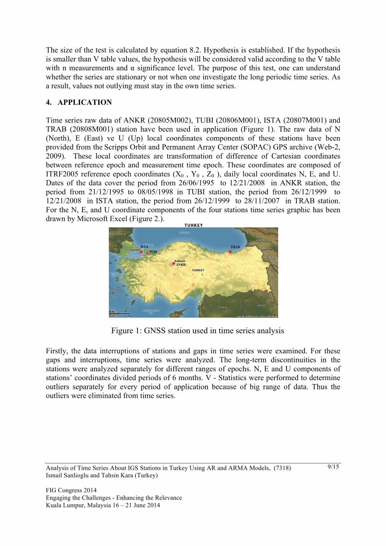
The size of the test is calculated by equation 8.2. Hypothesis is established. If the hypothesis is smaller than V table values, the hypothesis will be considered valid according to the V table with n measurements and α significance level. The purpose of this test, one can understand whether the series are stationary or not when one investigate the long periodic time series. As a result, values not outlying must stay in the own time series. 4. APPLICATION Time series raw data of ANKR (20805M002), TUBI (20806M001), ISTA (20807M001) and TRAB (20808M001) station have been used in application (Figure 1). The raw data of N (North), E (East) ve U (Up) local coordinates components of these stations have been provided from the Scripps Orbit and Permanent Array Center (SOPAC) GPS archive (Web-2, 2009). These local coordinates are transformation of difference of Cartesian coordinates between reference epoch and measurement time epoch. These coordinates are composed of ITRF2005 reference epoch coordinates (X0 , Y0 , Z0 ), daily local coordinates N, E, and U. Dates of the data cover the period from 26/06/1995 to 12/21/2008 in ANKR station, the period from 21/12/1995 to 08/05/1998 in TUBI station, the period from 26/12/1999 to 12/21/2008 in ISTA station, the period from 26/12/1999 to 28/11/2007 in TRAB station. For the N, E, and U coordinate components of the four stations time series graphic has been drawn by Microsoft Excel (Figure 2.).

Figure 1: GNSS station used in time series analysis Firstly, the data interruptions of stations and gaps in time series were examined. For these gaps and interruptions, time series were analyzed. The long-term discontinuities in the stations were analyzed separately for different ranges of epochs. N, E and U components of stations’ coordinates divided periods of 6 months. V - Statistics were performed to determine outliers separately for every period of application because of big range of data. Thus the outliers were eliminated from time series.


10/15

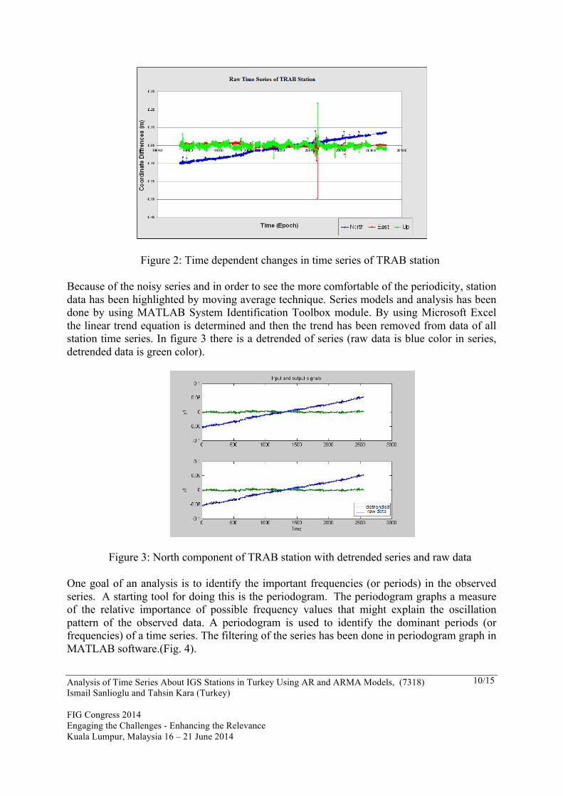
Figure 2: Time dependent changes in time series of TRAB station

Because of the noisy series and in order to see the more comfortable of the periodicity, station data has been highlighted by moving average technique. Series models and analysis has been done by using MATLAB System Identification Toolbox module. By using Microsoft Excel the linear trend equation is determined and then the trend has been removed from data of all station time series. In figure 3 there is a detrended of series (raw data is blue color in series, detrended data is green color).

Figure 3: North component of TRAB station with detrended series and raw data

One goal of an analysis is to identify the important frequencies (or periods) in the observed series. A starting tool for doing this is the periodogram. The periodogram graphs a measure of the relative importance of possible frequency values that might explain the oscillation pattern of the observed data. A periodogram is used to identify the dominant periods (or frequencies) of a time series. The filtering of the series has been done in periodogram graph in MATLAB software.(Fig. 4).


11/15

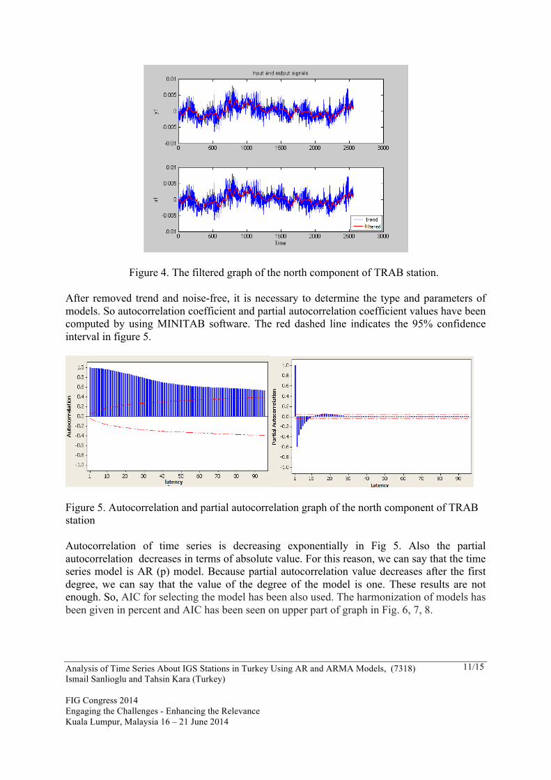
Figure 4. The filtered graph of the north component of TRAB station.

After removed trend and noise-free, it is necessary to determine the type and parameters of models. So autocorrelation coefficient and partial autocorrelation coefficient values have been computed by using MINITAB software. The red dashed line indicates the 95% confidence interval in figure 5.

Figure 5. Autocorrelation and partial autocorrelation graph of the north component of TRAB station Autocorrelation of time series is decreasing exponentially in Fig 5. Also the partial autocorrelation decreases in terms of absolute value. For this reason, we can say that the time series model is AR (p) model. Because partial autocorrelation value decreases after the first degree, we can say that the value of the degree of the model is one. These results are not enough. So, AIC for selecting the model has been also used. The harmonization of models has been given in percent and AIC has been seen on upper part of graph in Fig. 6, 7, 8.


12/15

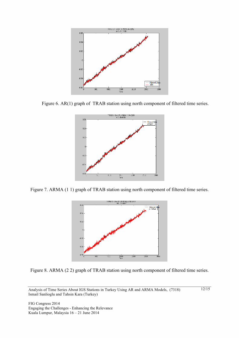
Figure 6. AR(1) graph of TRAB station using north component of filtered time series.

Figure 7. ARMA (1 1) graph of TRAB station using north component of filtered time series.

Figure 8. ARMA (2 2) graph of TRAB station using north component of filtered time series.


13/15

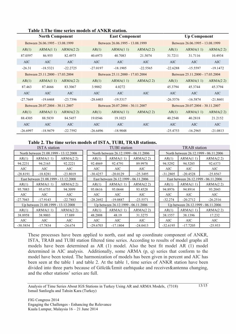
Table 1.The time series models of ANKR station. North Component East Component Up Component

Between 26.06.1995 - 13.08.1999 Between 26.06.1995 - 13.08.1999 Between 26.06.1995 - 13.08.1999

AR(1) ARMA(1 1) ARMA(2 2) AR(1) ARMA(1 1) ARMA(2 2) AR(1) ARMA(1 1) ARMA(2 2)

87.0597 86.955 82.4975 40.6973 40.7083 21.5074 31.7211 31.7116 10.4934

AIC AIC AIC AIC AIC AIC AIC AIC AIC

-26.31 -18.5321 -22.2725 -27.0197 -18.1905 -22.5565 -22.6288 -15.5597 -19.1472



87.463 87.4666 83.3067 3.9882 4.0272 45.3794 45.3744 45.3794


-27.7669 -19.6468 -23.7396 -28.6403 -19.5317 -26.5576 -16.5874 -21.8601



88.4305 88.5839 84.5457 19.0546 19.1023 40.2548 40.2818 21.2152


-26.6997 -18.9479 -22.7592 -26.6496 -18.9048 -25.4753 -16.2965 -21.0813

Table 2. The time series models of ISTA, TUBI, TRAB stations.

ISTA station

TUBI station

TRAB station North between 21.08.1999 - 13.12.2008

North between 26.12.1999 - 06.11.2006

North between 26.12.1999 - 06.11.2006

AR(1) ARMA(1 1) ARMA(2 2)


AR(1) ARMA(1 1) ARMA(2 2) 94.2231 94.2165 92.2221

92.4869 92.4791 89.9978

94.5292 94.5285 92.6373

AIC AIC AIC

AIC AIC AIC

AIC AIC AIC -28.8191 -18.8281 -23.8019

-30.4257 -20.0129 -25.3495

-31.2805 -20.4528 -25.8567

East between 21.08.1999 - 13.12.2008

East between 26.12.1999 - 06.11.2006

East between 26.12.1999 - 06.11.2006 AR(1) ARMA(1 1) ARMA(2 2)



95.7083 95.6755 94.3099

95.0616 95.0644 93.4528

94.8976 94.8914 93.2043 AIC AIC AIC

AIC AIC AIC

AIC AIC AIC

-27.7043 -17.9143 -22.7883

-28.2692 -19.0887 -23.5571

-32.274 -20.2712 -26.2516 Up between 21.08.1999 - 13.12.2008

Up between 26.12.1999 - 06.11.2006

Up between 26.12.1999 - 06.11.2006



AR(1) ARMA(1 1) ARMA(2 2) 38.8958 38.9003 17.889

48.2008 48.19 31.3275

38.1557 38.1396 17.232

AIC AIC AIC

AIC AIC AIC

AIC AIC AIC -30.5854 -17.7834 -24.674

-29.6703 -17.1804 -24.0413

-32.6195 -17.7205 -25.933

These processes have been applied to north, east and up coordinate component of ANKR, ISTA, TRAB and TUBI station filtered time series. According to results of model graphs all models have been determined as AR (1) model. Also the best fit model AR (1) model determined in AIC analysis. Additionally, some ARMA (p, q) series that conform to the model have been tested. The harmonization of models has been given in percent and AIC has been seen at the table 1 and table 2. At the table 1, time series of ANKR station have been divided into three parts because of Gölcük/İzmit earhtquake and receiver&antenna changing, and the other stations’ series are full.


14/15

5. CONCLUSIONS

As shown in the graph of time series, there are data discontinuities in time series for the hardware reasons, i.e. ANKR station. Thus we can say that these interruptions could adversely affect the results of time series analysis and analysis will result in incorrect results. So for the modeling of time series, the available data must be compatible with each other as possible and loss of data by the long-and short-term in series should not be. Also, data have to be obtained from a long-term series. If these rules are performed, better results can be achieved. AR and ARMA models has been used time series analysis of the stations and autocorrelation and partial autocorrelation coefficients of the AR (1) and ARMA (1 1) models the values are close to each other out. Degrees of northing and easting components are one degree in auto-regression and partial- auto-regression graphics and their autocorrelations are in downward tendency in the positive direction; and decreasing suddenly in the positive direction after the first degree, their partial-autocorrelations make small changes in both positive and negative directions. It can be said that these tendencies are consistent with the auto-regression model (AR), among the models of time series. Akaike Information Criterion has tested to model results and as a result the station data that they have made in the past period the movements, in the future to allow for the best interpretation of the model AR (1) that has been seen. REFERENCES Akaike, H, 1974, "A new look at the statistical model identification", IEEE Transactions on Automatic Control Volume:19, Issue:6, page 716–723, Akdeniz, H., A., 1998, Applied Statistics II, Nine September University, Faculty of Economics and Administrative Sciences, İzmir (in Turkish) Allen, R.G.D., 1964, Statics for Economists, MC - Millan, UK Altamimi Z., X. Collilieux, 2009, IGS contribution to ITRF, Journal of Geodesy, vol. 83, number 3-4, page 375--383, Bianchi, L., Jarrett, J., and Hanumara, R. C. , 1998, Improving forecasting for telemarketing centers by ARIMA modeling with intervention. International Journal of Forecasting 14, pp. 497-504 Caissy M., Agrotis L., Weber G., Hernandez-Pajares M., Hugentobler U., 2012, Innovation: The International GNSS Real-Time Service, GPS World, 23(6): 52-58. Fei, W. and Bai, L., 2014, Time-Varying Moving Average Model for Autocovariance Nonstationary Time Series, Journal of Fiber Bioengineering and Informatics 7:1 pp: 53-65 Feng, Y. ,2012, Regression and hypothesis tests for multivariate GNSS state time series. Journal of Global Positioning Systems, 11(1), pp. 33-45. Ferland R., 2006, Proposed IGS05 realization, IGS Mail 5447,


15/15

http://igscb.jpl.nasa.gov/mail/igsmail/2006/msg00170.html Ferland, R. and Piraszewski, M., 2009, The IGS-combined station coordinates, Earth rotation parameters and apparent geocenter. J. Geodesy, 83, 385-392, Imdadullah, M., 2013, Time Series Analysis and Forecasting, http://itfeature.com/time-series-analysis-and-forecasting/time-series-analysis-forecasting Li, J.; Miyashita, K.; Kato, T.; Miyazaki, S., 2000, GPS time series modeling by autoregressive moving average method: Application to the crustal deformation in central Japan, Earth, Planets and Space, Volume 52, p. 155-162. Mann, S. P., 1995, Statistics For Business and Economics, Wiley, USA Pang, C.,H., Lewis, F.,L., Lee, T.,H., Dong, Z.,Y., 2011, Intelligent Diagnosis and Prognosis of Industrial Networked Systems, CRC Press, Sincich, T., 1996, Business Statistics By Example, Prentice- Hall International Editions, fifth edition, USA Web-1, 2014, http://en.wikipins.org/c/Time_series_analysis Web-2, 2009, ftp://garner.ucsd.edu/pub/timeseries/ Yerci, M., 2002, Errors and Statistics, Selçuk University, Enginerring and Architecture Faculty Publications, (Lecturer Notes :6), Konya, in Turkish BIOGRAPHICAL NOTES CONTACTS İsmail ŞANLIOĞLU Selcuk University, Engineering Faculty, Department of Geomatics Alaeddin Keykubad Campus Selçuklu/Konya TURKEY Tel. +903322231940 Fax + 903322410635 Email:[email protected] Web site: http://www.harita.selcuk.edu.tr 1Selcuk University, Engineering Faculty, Geomatics Department, Selcuklu/Konya, TURKEY 2 General Directorate of Land Registry and Cadastre , Map Department, Çankaya/Ankara, TURKEY

Documents

Analysis of Time Series About IGS Stations In Turkey Using AR …fig.net/pub/fig2014/papers/ts09b/TS09B_sanlioglu_kara... · 2014-07-03 · Analysis of Time Series About IGS Stations