Embed Size (px)
Citation preview

1
Analysis of Ultra Low Cycle Fatigue problems with the Barcelona plastic damage model and a
new isotropic hardening law
X. Martineza,b,* , S. Ollera,c, L.G. Barbua,c, A.H. Barbata,c and A.M.P. de Jesusd,e
a. International Center for Numerical Methods in Engineering (CIMNE). Campus Nord, Gran Capità s/n, 08034 Barcelona, Spain
b. Department of Nautical Science and Engineering - UPC. Pla de Palau 18, 08003 Barcelona, Spain
c. Department of Strenght of Materials and Structural Engineering - UPC. Edifici C1, Campus Nord, Jordi Girona 1-3, 08034
Barcelona, Spain
d. IDMEC, Rua Dr. Roberto Frias, 4200-465 Porto, Portugal
e. Departamento de Engenharia Mecânica, Faculdade de Engenharia, Universidade do Porto, Rua Dr. Roberto Frias, 4200-465
Porto, Portugal
* Corresponding author. [email protected]
Key words: Ultra low cycle fatigue; plastic damage; isotropic hardening; kinematic hardening;
constitutive modelling
Abstract
This paper presents a plastic-damage formulation and a new isotropic hardening law, based on the
Barcelona plastic damage model initially proposed by Lubliner et al. in 1989 [1], which is capable of
predicting steel failure due to Ultra Low Cycle Fatigue (ULCF). This failure mechanism is obtained when
the material is subjected to cyclic loads and breaks after applying a very low number of cycles, usually
less than hundreds. The failure is driven by the plastic response of the material, and it is often
predicted based on the plastic strains applied to it. The model proposed in this work has been
formulated with the objective of predicting accurately the plastic behavior of the material, as well as its
failure due to ULCF. This is achieved taking into account the fracture energy dissipated during the
whole loading process. This approach allows the simulation of ULCF when it takes place due to regular
cyclic loads or non-regular cyclic loads, as it is the case of seismic loads. Several simulations are
conducted in order to show the capabilities of the formulation to reproduce the mechanical response
of steel when it is subjected to regular and non-regular cyclic loads. The formulation is validated
comparing the numerical results with several experimental tests made on X52 steel specimens. The
agreement between the numerical and experimental results asses the validity of the proposed model
to predict the plastic behavior of steel and its failure due to Ultra Low Cycle Fatigue.
1 INTRODUCTION
The mechanical phenomenon known as fatigue consists in the loss of material strength, and
consequent failure, due to the effect of cyclic loads. Fatigue is characterized, among other parameters,
by the number of cycles, load amplitude and reversion index ([2], [3] and [4]). Material failure is

2
produced by an inelastic behaviour, micro-cracking and crack coalescence, which lead to the final
collapse of structural parts.
Fatigue phenomenon is defined more generally in the ASTM E1823 standard as: "the process of
permanent, progressive and localized structural change which occurs to a material point subjected to
strains and stresses of variable amplitudes which produce cracks which lead to total failure after a certain
number of cycles" [5]. In this definition it is possible to include all fatigue ranges, from “Ultra Low Cycle
Fatigue” (ULCF), to “Low Cycle Fatigue” (LCF) and “High Cycle Fatigue” (HCF).
While there is a general agreement that for failures in the range of 106 to 108 cycles the structure has
failed in the high cycle fatigue range, there is not such agreement in defining the limits for low cycle
and ultra low cycle fatigue. Authors such as Kanvinde and Deierlein [6] consider that LCF is found
between 100s and 1000s cycles and that ULCF is in the range of 10-20 cycles; and other authors, such
as Xue [7], put these limits in 104 for LCF and 100 for ULCF. However, despite these discrepancies, there
is a general agreement that plastic behaviour of the material plays an important role in the failure due
to LCF or ULCF [8].
According to the literature review made by Yao and Munse in [9], first attempts to characterize LCF
and ULCF can be attributed to Kommers who, in 1912, conducted several tests on a cantilever
specimen subjected to cyclic bending. After these tests he reached the conclusion that the magnitude
of deflection plays an important role in low cycle fatigue. However, main efforts to characterize the
parameters driving LCF and ULCF are not found until 1950s, when numerous experimental programs
where carried out to calibrate the material constants for various metals. A large amount of work is
documented from this period. The experimental data is usually plotted on a log–log scale with the
abscissa representing the number of life cycles and the ordinate the plastic strain amplitude. This
graph is known as the p N curve. Following this approach, probably the most know, and most
widely used, procedure to predict material failure under LCF and ULCF is the Manson-Coffin law ([8],
[10], [11]):
CNp (1)
p being the plastic strain range in the material, N the number of cycles that can be applied
before ULCF and LCF failure, and and C material constants.
From this first equation proposed by Coffin and Manson, several authors have provided their own law
in order to improve the accuracy on the predicted cycles before failure, especially in the Ultra Low
Cycle Fatigue regime. For instance, Xue [7] observed, from experimental results, that the law did not fit
well in the range of very low life cycles, less than 100, so he proposed a new exponential damage rule
that improved this accuracy. Kuroda [11] also provided a modification on the original Coffin-Manson
law in order to predict the failure below 100 cycles. In this case the model is based on the
accumulation of damage due to three different effects: tensile straining, cyclic straining and crack
propagation.

3
The approach used by Tateishi et al. [12] to simulate LCF failure is also interesting. These authors use
Miner’s rule to couple the effect of high cycle fatigue with the effect of low cycle fatigue, by adding a
ductile damage term. This last term depends on the yield strain of the material, the rupture strain and
the strain that is applied in a given cycle.
One of the main drawbacks of most of the existing formulations to characterize ULCF and LCF is that
they require regular cycles to predict material failure, or they couple the effects of non-regular cycles
using the Miner’s rule, which requires knowing the performance of the structure under regular cycles.
However, this regularity often does not exist. An example of an ULCF failure due to an irregular cyclic
load is found in the failure of structures subjected to seismic loads, where the frequency varies along
time and each cycle may have different amplitudes.
An interesting approach to characterize low cycle fatigue accounting for non-regular cycles is the one
proposed by Jiang et al. [13], which defines an independent continuous cumulative damage function
(EVICD) based on the accumulation of plastic strain energy. This formulation is based on previous
models of EVICD ([14], [15] and [16]) and states that the total damage can be computed as:
pdWdDwithdDD (2)
being D the fatigue damage, pW the plastic strain energy density and a function determined
experimentally based on the fatigue response of the material. With this approach, the authors obtain
an evolution of the fatigue damage parameter as the simulation evolves, the material failure is
obtained when 1D . In [13], the model is tested for fatigue ranges between 103 to 107 cycles, which
corresponds to low and high cycle fatigue.
Another interesting approach based on damage accumulation is the one proposed by Kanvinde and
Deierlein ([6], [17], and [18]). These authors, in order to account for the effects of void growth and
coalescence that drive the fracture of metallic materials, propose a model that calculates the void
growth and compares it with a critical value to detect material failure. This parameter is obtained
experimentally. The initial formulation developed for monotonic cases (Void Growth Model - VGM
[17]) is extended to cyclic loads by differentiating the void growth obtained in the tensile and
compressive regions of the load cycle. Therefore, the void growth in the Cyclic Void Growth Model
(CVGM) can be obtained as [18]:
critical
cyclic
cyclesecompressiv
p
e
m
cyclestensile
p
e
m
cyclic
VGIdC
dCVGI
2
1
2
1
5.1exp
5.1exp
2
1
(3)
This formulation, as well as the formulation proposed by Jiang et al. [13], are capable to account for
regular and non-regular cycles, as both formulations are based on the addition of certain quantities
4
while the material increases its plastic strain. However, they both have the drawback of being based on
a failure criterion that is completely independent of the plastic model (uncoupled approaches): it is
calculated as the simulation advances and, when it reaches a certain level, the criterion tells the code
that the material has failed.
The simulation of LCF and ULCF has also been approached using non-linear constitutive laws. This is
the case of Saanouni and Abdul-Latif ([19], [20]), who propose the use of a representative volume
element (RVE), and a non-linear law based on the slip theory, to account for the dislocation movement
of metallic grains. Instead of a RVE, Naderi et al. [21] proposed simulating the progressive failure of a
given structural element by applying random properties to the different finite elements in which it is
discretized. The constitutive model used to characterize LCF failure is the one defined by Lemaitre and
Chaboche in [22]. The use of a stochastic approach is also the approach used by Warhadpande et al.
[23], who applied random properties to a Voronoi cell. In most of these models the damage variable is
also calculated independently of the non-linear constitutive law used to simulate the material
performance.
Current work proposes the use of a plastic damage model, and presents a new isotropic hardening
law, to simulate Ultra Low Cycle Fatigue. The model developed is based on the Barcelona model
originally formulated by Lubliner et al. ([1], [24], [25] and [26]). Although this model was originally
defined to simulate brittle materials such as concrete, here is used with a kinematic and isotropic
hardening law specifically defined for the simulation of steel. The isotropic hardening law is defined
with an initial hardening region followed by a softening region. One of the main characteristics of the
model is that the isotropic hardening behaviour of the material is driven by the plastic energy
dissipated: the model measures the fracture energy that is dissipated as the plastic strain increases,
and this energy is used to define the plastic strain level at which material softening due to damage
starts and finishes. The model considers that damage initiates when the plastic law reaches the
softening region and the complete failure is obtained when all fracture energy of the material is
dissipated. A first preliminary description of the procedure used by the proposed model has been
already presented in [27] and [28].
This work proves that the proposed model it capable of simulating material failure due to Ultra Low
Cycle Fatigue by its own, without the need of any other damage variable computed independently of
the plastic formulation. Besides, the proposed approach is not only capable of predicting material
failure for regular and non-regular cyclic loads, but it is also capable of coupling cyclic loads with
monotonic loads, which allows to predict that the structure will fail sooner if the monotonic load is
applied after several hysteresis cycles, than if these cycles are not applied. This capability is obtained as
a consequence of the fact that the material failure is predicted by the plastic non-linear constitutive
equation itself. Another advantage of the formulation proposed is that it is capable of using any yield
and potential surfaces to characterize the material, which increases its applicability to different steel
alloys.

5
2 PLASTIC DAMAGE MODEL
The inelastic theory of plasticity can simulate the material behavior beyond the elastic range, taking
into account the change in the strength of the material through the movement of the yield surface,
representing isotropic and kinematic hardenings. It is assumed that each point of the solid follows a
thermo-elasto-plastic constitutive law (stiffness hardening/softening) ([1], [29] and [30]) with the stress
evolution depending on the free strain variable and plastic internal variables. The formulation
presented hereafter studies the phenomenon of stiffness degradation accumulation through a plastic-
damage law.
2.1 Plastic Model
Since this work is guided to mechanical problems with small elastic strains and large inelastic strains,
the free energy additively hypothesis is accepted pe ([31], [32]). The elastic
e and plastic
p parts of the free energy are written, in the reference configuration for a given entropy and
temperature field, as the elastic Green strains ij
p
ijij
e
ij EEEE ; the two last variables operate
as free field variables ([29], [32] and [33]). The free energy is thus written as,
),(2
1),(),( ppe
klijkl
e
ij
ppe
ij
e ECEm
E (4)
Considering the second thermodynamics law (Clausius-Duhem inequality, [31], [34] and [35]), the
thermo mechanical dissipation can be obtained as [32]:
01
i
p
p
p
ijijq
mm
ES
(5)
The accomplishment of this dissipation condition, equation (5), demands that the expression of the
stress and the entropy should be defined as (Coleman method; see [35]);
;e
klijkle
ij
e
ij ECE
mS (6)
From the last expression is possible to obtain the general expression of the tangent constitutive tensor,
e
kl
e
ij
e
e
ij
ijt
ijklEE
mE
SC
2 (7)
In equations (4) to (7), m is the material density, ijE , e
ijE , p
ijE are the total, elastic and plastic strain
tensors, respectively, ijS is the stress tensor for a single material point, ijklC and t
ijklC are the initial
and tangent constitutive tensors, and p are the plastic internal variables.

6
2.2. Yield plastic functions
The yield function F accounts for the residual strength of the material, which depends on the current
stress state, the temperature and the plastic internal variables. This F function and the plastic
potential G have the following form, taking into account isotropic and kinematic plastic hardening
(Bauschinger effect; [22], [36] and [37]),
cteSgSG
SKSfSF
ijij
p
ij
p
ijijij
p
ij
)(),,(
0),,()(),,(
(8)
where )( ijijSf and )( ijijSg are the uniaxial equivalent stress functions depending on the
current value of the stresses, ijS , and the kinematic plastic hardening internal variable, ij ;
),,( p
ijSK is the plastic strength threshold, p is the plastic isotropic hardening internal variable,
and is the temperature at current time t ([1], [29] and [30]).
The evolution law for the plastic strain is obtained from the evolution of the plastic potential as,
ij
pp
ijS
GE
(9)
where is the plastic consistency parameter. We will talk of associated plasticity when the plastic
potential is the same as the plastic yield function, which is the assumption followed in this research.
2.3 Kinematic Hardening
Kinematic hardening accounts for a translation of the yield function allowing the representation of the
Bauschinger effect in the case of cyclic loading. A two dimensional representation of this movement in
the 21 SS plane is shown in the following figure:
Figure 1. Translation of the yield surface as a result of kinematic hardening
This translation is driven by the kinematic hardening internal variable ij which, in a general case,
varies proportionally to the plastic strain of the material point ([22], [38]). There are several laws that

7
define the evolution of this parameter. Current work uses a non-linear kinematic hardening law, which
can be written as:
pdEc ijk
P
ijkij (10)
where kc and kd are material constants, p
ijE is the plastic strain, and p is the increment of
accumulated plastic strain, which can be computed as: p
ij
p
ij EEp :3/2 . Note that the 2/3 is valid
in case of using Von-Mises as the actual yield surface. In other cases, this value should be modified.
2.4 Isotropic Hardening
Isotropic hardening provides an expansion or a contraction of the yield surface. The expansion
corresponds to a hardening behaviour and the contraction to a softening behavior. In the following
figure a two dimensional representation of this effect in the 21 SS plane is depicted:
Figure 2. Expansion of the yield surface as a result of isotropic hardening
The evolution of isotropic hardening is controlled by the evolution of the plastic hardening function K ,
which is often defined by an internal variable p . The rate equation for these two functions may be
defined, respectively:
pp
p
kk
EhS
GhH
hHK
kk :
k
(11)
where k denotes scalar and k states for a tensor function. Depending on the functions defined to
characterize these two parameters different material performances can be obtained. A new function to
characterize metallic materials is proposed in this work and described in Section 3 of this document.

8
2.5. Stress-strain relation and consistency factor
Once the material has exceeded its yield threshold stress, the stress-strain relation is defined by the
tangent stiffness tensor. The expression of this tensor, as well as the expression of the plastic
consistency parameter can be obtained from the plastic yield criterion and the Prager consistency
condition [38]:
0
0
0),,()(),,(
KF
SS
F
KK
FFS
S
FF
SKSfSF p
ijijij
p
ij
(12)
Using previous expressions, it is possible to rewrite equation (12) as:
0::::
p
kijk
P
ijk
p EhhpdEcF
EECS
F k
(13)
From this expression it is possible to obtain the consistency factor using equation (9):
0:::::::
S
Ghh
S
GFc
S
GC
S
Fpd
FEC
S
Fkkijk k
(14)
Therefore:
S
Ghh
S
GFc
S
GC
S
F
ECS
F
kk
ijk
::::
:::
k
(15)
The tangent stiffness tensor relates the total strain rate to the stress rate:
ECS t : (16)
Finally, the expression of the tangent stiffness tensor can be obtained from the consistency factor:
S
Ghh
S
GFc
S
GC
S
F
CS
F
S
GC
CC
kk
t
::::
::
k
(17)
It has to be noted that expression (17) has been obtained disregarding the non-linear term of
kinematic hardening. Despite having a first approximation of the analytical expression that provides
the tangent stiffness tensor, in many occasions the calculation of the partial derivatives of the yield and
potential functions is not straightforward. In those cases, a numerical derivation can be performed. This
procedure, although expensive, provide an accurate approximation that improves the global
convergence of the problem. An efficient procedure to conduct this numerical derivation, as well as the

9
advantages obtained with it, are shown in [39]. A detailed description of the integration procedure of
the constitutive equations can be found in references [32] and [38].
3 NEW ISOTROPIC HARDENING LAW
Equation (11) allows the incorporation of different hardening laws to describe the material
performance. In the Barcelona model defined in [1], the laws defined are driven by the fracture energy
of the material. This work presents a new law, specially developed for steel materials, that has been
designed to reproduce their hardening and softening performance under monotonic and cyclic
loading conditions. This law also depends on the fracture energy of the material.
3.1 Fracture Energy
Classical fracture mechanics defines the fracture energy of a material as the energy that has to be
dissipated to open a fracture in a unitary area of the material. This energy is defined as:
f
f
fA
WG (18)
where fW is the energy dissipated by the fracture at the end of the process, and fA is the area of
the surface fractured. The total fracture energy dissipated, fW , in the fracture process can be used to
define a fracture energy by unit volume, fg , required in a continuum mechanics formulation:
fV
ffff dVgAGW (19)
This last equation allows establishing the relation between the fracture energy defined as a material
property, fG , and the maximum energy per unit volume:
f
f
ff
f
f
f
fl
G
lA
W
V
Wg
(20)
Thus, the fracture energy per unit volume is obtained as the fracture energy of the material divided by
the fracture length. This fracture length corresponds to the distance, perpendicular to the fracture area,
in which this fracture propagates.
In a real section, this length tends to be infinitesimal. However, in a finite element simulation, in which
continuum mechanics is applied to a discrete medium, this length corresponds to the smallest value in
which the structure is discretized: the length represented by a gauss point.

10
Therefore, in order to have a finite element formulation consistent and mesh independent, it is
necessary to define the hardening law in function of the fracture energy per unit volume ([1], [30], [40]
and [41]). This value is obtained from the fracture energy of the material, fG , and the size of the finite
element in which the structure is discretized.
3.2 Hardening Function and Hardening Internal Variable
The hardening function defines the stress of the material when it is in the non-linear range. There are
many possible definitions that can be used for this function fulfilling equation (11). Among them, here
it is proposed to use a function that describes the evolution of an equivalent uniaxial stress state, like
the one shown in Figure 3.
This equivalent stress state shown in Figure 3 has been defined to match the uniaxial stress evolution
described by most metallic materials. After reaching the yield stress, the curve is divided in two
different regions. The first region is defined by curve fitting from a given set of equivalent stress-
equivalent strain points. The curve used to fit the points is a polynomial of any given order defined
using the least squares method. The data given to define this region is expected to provide an
increasing function, in order to obtain a good performance of the formulation when performing cyclic
analysis.
Figure 3. Evolution of the equivalent stress
The second region is defined with an exponential function to simulate softening. The function starts
with a null slope that becomes negative as the equivalent plastic strain increases. The exact geometry
of this last region depends on the fracture energy of the material. The adjustment of this exponential
softening to experimental results is usually very difficult, as the stress drop is very fast and
experimental tests cannot capture it. Therefore, its definition will be done just to obtain a more or less
steep slope. The selection of an exponential function instead of a straight line or a polynomial is made
because the exponential function provides a response that facilitates the numerical convergence.
It has to be noted that the initial plateau that is usually found in monotonic stress-strain graphs of
carbon steels is not represented in the stress evolution proposed in this model and, therefore, it is not
shown in Figure 3. This is because the definition of this region will lead to inaccurate results when
performing cyclic simulations of the material.

11
The hardening internal variable, p , accounts for the evolution of the plastic hardening function, K .
In current formulation p is defined as a normalized scalar parameter that takes into account the
amount of volumetric fracture energy dissipated by the material in the actual strain-stress state. This is:
dtESg
t
t
p
f
p
0
:1 (21)
Figure 4 shows shaded in green the volumetric fracture energy required by a uniaxial loaded material,
for a given plastic strain, pE , to start the material softening. The hardening internal variable defined
in (21) is calculated normalizing this fracture energy by the total fracture energy of the system, fg ,
which corresponds to the total area below the curve )( peq ES , shaded with parallel lines.
Figure 4. Representation of the volumetric fracture energy of a metallic material
Using the definition of the hardening internal variable defined in equation (21), it is possible to define
the expression of the hardening function as:
)( peqSK (22)
It can be easily proven that the hardening function and internal variable defined in equations (21) and
(22) fulfill the rate equations (11). The kh and kh functions defined in expression (11) become:
t
p
eq
k
g
Sh
Sh
k
(23)
3.3 Expressions of the hardening function
In this section the exact numerical expressions used to define the new hardening law presented in this
work are provided. This law is characterized with two different functions, each one defining the
evolution of the equivalent stress in each region in which the equivalent stress performance is divided
(see Figure 3).

12
Region 1: Curve fitting with polynomial
The first region is characterized with a polynomial defined by curved fitting from a given experimental
data. Among the different available methods that can be used to define this polynomial, here is
proposed to use the least squares method due to its simplicity, computational cost, and good
performance provided. The resulting relation between the stress and plastic strain in this region is:
ipN
i
i
peq EaaES
1
0)( (24)
with N the order of the polynomial.
The volume fracture energy that is dissipated in this region can be obtained calculating the area below
the peq ES graph. This calculation provides the following value:
1
1
121
N
i
ipipit EE
i
ag (25)
being pE1 and
pE2 the initial and final plastic strain values, respectively, that limit the polynomial
function region.
Although the equivalent plastic stress should depend on the plastic internal variable p , in a cyclic
simulation with isotropic hardening, this approach will produce hysteresis loops with increasing stress
amplitude (for a fixed strain amplitude). For this reason, current formulation calculates the equivalent
plastic stress using the value of the equivalent plastic strain, which is obtained as:
)(
:
Sf
ESE
pp (26)
with )(Sf defined by the yield surface used to simulate the material, as it is shown in equation (8).
Finally, the derivative of the hardening function can be calculated with the following expression:
1
1
1
1
1
1
N
i
ip
i
N
i
ip
i
tp
p
p
eq
p
eq
Ea
Eai
gd
dE
dE
dS
d
dS
(27)
Expression (27) is valid for values of p that are comprehended between 01 p and tt
p gg 12 .
The value of the upper limit of the internal variable shows that it is necessary to define a value for the
volumetric fracture energy of the material larger than 1tg . If the value defined is lower, the material
will not be able to reach its ultimate stress as this will imply having a fracture internal variable larger
than 0.1 .

13
Region 2: Exponential softening
When the plastic internal variable reaches the volumetric plastic energy available for the first region,
pp
2 , isotropic hardening follows region two. The function that defines this new region is defined
with the following parameters:
1. The initial equivalent stress value is defined by the equivalent stress reached in the first region
(eqS2 ). This value can be the one defined in the material characterization or can be a lower
value if there has been some plastic energy dissipation in a cyclic process. In this last case, the
stress value has to be obtained from the previous region.
2. The initial slope of the function is zero.
3. The volumetric fracture energy dissipated in this region is the remaining energy in the
material:
12 ttt ggg
With these considerations in mind, the resulting equation that relates the equivalent stress with the
plastic strain is:
pppp EEbEEbeqpeq eeSES 22 2
2 2)(
(28)
where
2
2
2
3
t
eq
g
Sb
The expression of the equivalent stress as a function of the hardening variable is obtained combining
equations (28) and (21), resulting:
2)( 2
eqpeq SS (29)
being, 12)(
2
2
eq
t
pp
S
gb
And the derivative of the hardening function is:
1
12
tp
eq
gbd
dS (30)
14
4 VALIDATION OF THE PROPOSED FORMULATION
In the following, the results obtained from several simulations conducted to validate the formulation
previously presented are included. This validation has been done comparing the numerical results with
some of the experimental results obtained in the framework of the Ultra Low Cycle Fatigue Project
([42]).
4.1 Description of the experimental tests
Monotonic and cyclic tests were performed in a close-loop servo-hydraulic machine, INSTRON 8801,
rated to 100 kN. The tests were performed at room-temperature in air. The fatigue tests were
conducted under constant strain amplitudes and with a frequency adjusted to result an average strain
rate of 0.008s-1. The longitudinal strain was measured using a clip gauge with limit displacements of
±2.5 mm with a gauge length of 12.5 mm (INSTRON 2620-602). This clip gauge was also used in two
monotonic tensile tests allowing the registration of the longitudinal strains until approximately 17%.
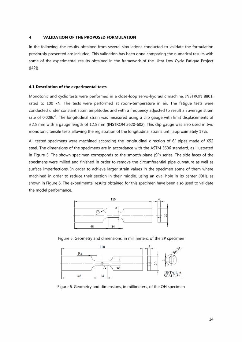
All tested specimens were machined according the longitudinal direction of 6″ pipes made of X52
steel. The dimensions of the specimens are in accordance with the ASTM E606 standard, as illustrated
in Figure 5. The shown specimen corresponds to the smooth plane (SP) series. The side faces of the
specimens were milled and finished in order to remove the circumferential pipe curvature as well as
surface imperfections. In order to achieve larger strain values in the specimen some of them where
machined in order to reduce their section in their middle, using an oval hole in its center (OH), as
shown in Figure 6. The experimental results obtained for this specimen have been also used to validate
the model performance.
Figure 5. Geometry and dimensions, in millimeters, of the SP specimen
Figure 6. Geometry and dimensions, in millimeters, of the OH specimen

15
4.2 Description of the numerical models
Two different numerical models have been defined, one for each experimental specimen. Figure 7
shows the meshes of both models. The SP model is made with 1608 quadratic hexahedral elements
and 8839 nodes. It has three elements along its thickness and 563 elements on the face shown in
Figure 7 (YZ plane). The OH model has 3080 quadratic hexahedral elements and 15460 nodes. It has
five elements along the thickness and 616 elements in the YZ face. This second model requires nearly
doubling the number of elements because the element size has to be significantly smaller around the
hole for its correct simulation. The SP model has marked two red dots that were used to calculate the
applied strain.
Figure 7. Meshes defined for the SP and OH numerical models.
As boundary conditions, the left border of the model has the displacement fixed to zero in all its
directions, while the right border is moved with an imposed displacement in the sample longitudinal
direction. The reaction force is obtained as a result of the numerical analysis.
All samples analyzed are defined with the same plastic material, defined with an associated plasticity
and Von-Mises as yield law. The material properties are obtained with the calibration process that is
described in the following section. All the material properties required by the model are displayed in
Table 1. A parameter of this table that may seem surprising is the value of the yield stress, which is
lower than the one expected for an X52 steel. This value is required because, if the yield stress is
defined with a higher value, the kinematic hardening parameters lead to stress values too high in the
hysteresis cycles. As the purpose of the model is the simulation of ULCF, which requires large plastic
strain values, the requirement of defining a lower yield stress is not considered a major drawback. This
yield stress does not represent the real material property but a numerical model parameter optimized
to improve the description of the cyclic elasto-plastic behavior of the material.
The hardening region is defined with a polynomial of order five which is computed with the least
squares method using available the experimental data. The constants of this polynomial, following
notation shown in equation (24), are shown in Table 2. In order to define the polynomial constants, it
has been necessary to take into account that the effects of the kinematic and the isotropic hardening
laws are coupled. This implies that the definition of the first region of isotropic hardening cannot be
obtained from the experimental curve straightforward, as this curve does not take into account the
displacement of the yield surface due to the kinematic hardening law.

16
Table 1. Numerical model parameters proposed for the X52 steel
Young Modulus 180 GPa
Poisson Ratio 0.30
Yield Stress (eq
Y ) 240 MPa
Plastic Strain threshold (pE2 ) 13 %
c1 kinematic hardening param. 60 GPa
d1 kinematic hardening param. 280
Fracture Energy ( fG ) 1.9 MN·m/m2
Table 2. Polynomial constants used to describe the hardening region of X52 material (Pa)
0a 2.4000E+08
1a 8.0084E+07
2a -1.1143E+08
3a 8.7400E+07
4a -3.0507E+07
5a 3.9073E+06
4.3 Calibration of the numerical model
The material data previously exposed has been obtained by model calibration. This is, adjusting the
different parameters required by the model to obtain a good fitting with one of the experimental
results available. For the current case, the experimental results considered are those of the SP
specimen loaded with an imposed strain range of 2.75%.
The results used to conduct the material calibration are the equivalent stress-equivalent strain graph
obtained from the experimental test. The stress is computed as the total force applied to the specimen
divided by the area of the cross section. The strains are computed dividing the measured displacement
of the clipped gauge by the length of the gauge. In the numerical model these two parameters were
calculated following the same procedure, using the red dots depicted in Figure 7.
The initial material parameters used in the calibration process are the ones commonly found in
literature and the polynomial constants correspond to the ones obtained by curve fitting of the
experimental results, ignoring the effect of kinematic hardening. Based on the strain-stress graph
obtained with these first values, the different parameters shown in Table 1 and Table 2 have been
modified (trial and error iterative procedure) until obtaining a numerical result that fits the
experimental results.
Figure 8 shows the stress-strain graph provided by the two experimental samples tested and by the
numerical model, which uses the material parameters obtained from the calibration process and

17
described in Table 1 and in Table 2. As it can be seen, the agreement in the cyclic behavior of the
numerical and experimental samples is rather good. This agreement is not achieved in the first
monotonic loading excursion, as the model developed is not prepared to reproduce the initial plateau
defined by the material. However, this disagreement is not considered relevant, as the model has been
developed thinking on the cyclic behavior and the evolution of plastic response for larger plastic strain
values, found beyond this initial plateau.
Figure 8. Stress-strain graphs for the SP sample with an applied deformation range of 2.75%
The fitting of the stress-strain graph allows defining all material parameters except the fracture energy
of the material and the equivalent plastic strain value at which softening is expected to start (pE2 ).
These two parameters have been defined to match the number of cycles that can be applied to the
specimen before it fails (inverse calibration). In the experimental campaign, the first specimen failed
after 150 cycles, and the second specimen failed after 103 cycles. To match these values, the numerical
model has been defined with a maximum hardening strain (pE2 ) of a 13%. Afterwards, the material
fracture energy parameter, fG , is fitted until finding a value that predicts the failure of the numerical
specimen after 128 cycles. These values are shown in Table 1 and used in the numerical simulations.
Material failure is found when some gauss points reach a plastic damage value close to one. At this
stage the numerical analysis cannot reach convergence and the specimen can be considered to be
completely broken. In current simulation, the convergence is lost for a p value close to 0.9, as it is
shown in Figure 9, where the value of plastic damage is represented in the last tensile and compressive
stages.

18
Figure 9. Values of p for the SP sample with an applied deformation range of 2.75%, when applying
the maximum tensile and compression strain before ULCF failure. Deformation is magnified by 20.
The mechanical performance of the numerical specimen along the simulation is shown in Figure 10,
where the stress-strain loops for different cycles are represented. This figure shows that the effect of
material softening in the specimen consists in a reduction of the equivalent stress obtained as the
number of cycles applied to the specimen increase. The figure also shows that softening has already
started in cycle 60, although the difference between the first loop and loop 60 is very small. In further
cycles the effect of softening becomes more visible, until material fails in cycle 128, where the
reduction of equivalent stress is close to a 20%. Figure 9 also shows that the strain amplitude increases
with the number of cycles applied to the specimen. This increase is obtained because equivalent strain
is calculated as the relative displacement of two given nodes (red dots in Figure 7), divided by the
original length between both nodes, and does not take into account that it is modified due to the
plastic deformations existing in the whole specimen.
Figure 10. Evolution of the stress-strain relation for different cycles of the SP numerical analysis.
19
The results obtained with the calibration model prove that the constitutive law proposed can be
adjusted to any given stress-strain law by adjusting properly the material parameters. The calibration
model has also been used to show the numerical and mechanical performance of the formulation
developed. The prediction capacity of the model will be shown in further simulations, in which the
material parameters are fixed and are used to analyze different specimens and load cases.
4.4 Validation of the developed theory
After having calibrated the material parameters, the rest of experimental tests available have been
simulated in order to compare the ULCF failure prediction made by the numerical model with the
results obtained from the experimental campaign. The constitutive model proposed in this work will
succeed if it is capable of representing accurately the equivalent stress-strain graphs for the different
deformation ranges tested experimentally and, even more important, if it is capable of predicting the
number of cycles that can be applied to the specimen before its failure.
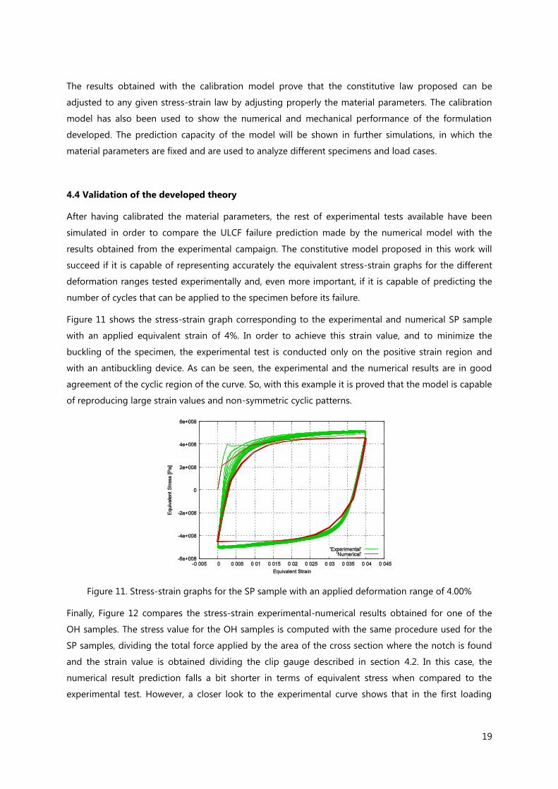
Figure 11 shows the stress-strain graph corresponding to the experimental and numerical SP sample
with an applied equivalent strain of 4%. In order to achieve this strain value, and to minimize the
buckling of the specimen, the experimental test is conducted only on the positive strain region and
with an antibuckling device. As can be seen, the experimental and the numerical results are in good
agreement of the cyclic region of the curve. So, with this example it is proved that the model is capable
of reproducing large strain values and non-symmetric cyclic patterns.
Figure 11. Stress-strain graphs for the SP sample with an applied deformation range of 4.00%
Finally, Figure 12 compares the stress-strain experimental-numerical results obtained for one of the
OH samples. The stress value for the OH samples is computed with the same procedure used for the
SP samples, dividing the total force applied by the area of the cross section where the notch is found
and the strain value is obtained dividing the clip gauge described in section 4.2. In this case, the
numerical result prediction falls a bit shorter in terms of equivalent stress when compared to the
experimental test. However, a closer look to the experimental curve shows that in the first loading

20
branch the experimental and numerical tests match perfectly, and it is in further cycles that the
experimental test provides larger equivalent stress values. This difference between hysteresis loops are
explained by an initial isotropic hardening of the material, for high cyclic plastic strain ranges
experienced by the material around the notch (oval hole), which cannot be captured by the proposed
model since the isotropic hardening was calibrated for lower plastic strain ranges, where this
hardening effects are not so pronounced. Since the material shows an isotropic hardening that is
dependent on the plastic strain range experienced by the material, the calibration of the material
should take into account the expected range of plastic strain ranges to be simulated. Despite this
difference, results are considered similar enough to validate the material parameters defined in the
numerical model calibration.
Figure 12. Stress-strain graphs for the OH sample with an applied deformation range of 1.25%
Once having proved that the developed formulation is capable of reproducing the mechanical
response obtained with the experimental samples, the following step is to verify if the formulation is
capable of predicting the failure of the specimens due to Ultra Low Cycle Fatigue. This validation is
performed counting the number of cycles that can be applied to the numerical model before its failure.
The numerical model is considered to fail when the convergence of the analysis is lost. This occurs
when some gauss points reach a p value close to 1.0. The number of cycles applied to the numerical
model are compared with the cycles obtained in the experimental campaign.
Figure 13 shows the results obtained for the SP samples. Results with reversion strain factor of –1 and
of 0 are plotted together because the reversion factor does not play a significant role in the material
response to ULCF. This figure shows that the number of cycles to failure predicted by the numerical
simulation are in very good agreement with the number of cycles obtained in the experimental
campaign. The only value that is not contained between the experimental results is the one
corresponding to an applied strain range of 3.5%. However, the value provided by the numerical
simulation looks more coherent than the one obtained with the experimental test, as the number of
cycles obtained in the experimental test is larger than the one obtained for an applied strain range of
2.75%.

21
Figure 13. ULCF failure prediction for SP specimens
The results obtained for the OH samples are shown in Figure 14. For these samples the experimental
test was conducted in just one specimen for each strain value, therefore there is no possibility of
knowing the scatter expected in the experimental tests. However, the number of cycles predicted by
the formulation is, for all strains, in the same order of magnitude than the experimental results
obtained. Therefore, it can be concluded that the formulation is, again, capable of predicting
accurately the ULCF failure of the OH specimens.
Figure 14. ULCF failure prediction for OH specimens
It is important to remark that the material properties used for all numerical simulations are exactly the
same. Therefore, the variation in the prediction of the number of cycles that can be applied to any of
the specimens considered is a result of the energy dissipated in each case. The agreement obtained in
all cases, independently of the reversion factor or the stress concentrations due to the existing oval
hole (OH specimens) allows considering the approach used to characterize ULCF failure an excellent
option. Moreover the formulation allows conducting simulations in which the cycles can be non-
regular, with varying amplitude and frequency, in which there can be sustained monotonic loads
between cycles or, in general, in which the load applied is not a regular one. This capability is not
offered by any other formulation available.

22
4.5 Advantages of the approach proposed
Previous results have shown that the proposed constitutive model is capable of predicting material
failure after applying several cycles to the material. However, this prediction capability does not
present a major advantage compared to other approaches such as the Coffin-Manson rule, or any
other analytical expression capable of defining the maximum number of cycles that can be applied for
a given plastic strain.
The main advantage of the proposed approach is that the prediction of ULCF failure does not depend
on the applied plastic strain, but on the energy dissipated during the cyclic process. Therefore, it is
possible to vary the plastic strain in the cycles applied to the structure and the constitutive model will
still be capable of predicting the material failure.
This is proved in the following example, where an irregular load, in frequency and amplitude, is applied
to the SP specimen defined in Section 4.2 and used to validate the formulation. The load defined is
depicted in Figure 15a. This load is applied as a fixed displacement following the same procedure used
for the SP specimen. The stress strain graph obtained from the numerical model is plotted in Figure
15b. As it can be seen, the applied load produces several loops, each one with a different plastic strain.
(a)
(b)
Figure 15. Seismic-type load applied (a) and material stress-strain response (b)
The model is capable of capturing the energy dissipated in each one of these loops and, therefore, to
evaluate the energy available in the material after having applied the load, which is equivalent to the
residual strength of the material. It is also possible to repeat several times the irregular load block,
shown in Figure 15a, to study the number of repetitions that are required to reach material failure.
Figure 16b shows the stress-strain response of the material after 10 blocks similar to the Figure 15a
(Figure 16a). At this point, there are some points in the model that have lost most of their fracture
strength and specimen failure occurs. As occurred with the SP model, this simulation also shows some
lateral displacement on the equivalent strains due to the plastic strains suffered by the whole
specimen.

23
(a)
(b)
Figure 16. Response of the model after ten seismic-type cycles: a) displacement-time history; b) stress-
strain history.
5 CONCLUSIONS
This work has presented a new plastic-damage formulation specially developed to simulate the
mechanical response of steel, and its failure due to Ultra Low Cycle Fatigue (ULCF). The formulation is
based on the Barcelona plastic model initially proposed by Lubliner et al. [1], which has been improved
by adding a non-linear kinematic hardening law coupled with a new isotropic hardening law. The
isotropic hardening law is divided in two regions. In the first one the steel exhibits a hardening
behavior, this region is defined by several points that have to be obtained from experimental tests.
And, in the second region, the steel has a softening behavior, which is defined with an exponential law.
The evolution of the material in these two regions is driven by the fracture energy that can be
dissipated by the material.
This approach allows predicting material failure by the constitutive model on its own, without the need
of additional parameters or additional laws specially chosen for the failure criteria that wants to be
simulated. Therefore, with the proposed formulation it is possible to simulate accurately the
mechanical response of steel under different loading scenarios, such regular or ramdom cyclic loading.
This last case is equivalent to the load that will be obtained in a seismic case, where ULCF may be one
of the main causes of structural failure. Several numerical analyses have been performed in order to
show the behavior of the formulation under the different loading scenarios mentioned.
The capacity of the formulation to simulate accurately the ULCF phenomenon has been proved by
reproducing different experimental tests made on X52 steel samples. The experimental campaign
consisted in loading several smooth specimens with different strain amplitudes. Tests were also
performed to notched specimens in order to increase the plastic strain and reduce the number of
cycles that could be applied before failure. One of the experimental tests has been used to calibrate
the material parameters of the model; afterwards all other specimen behaviors have been reproduced

24
numerically. All the numerical results obtained with the proposed constitutive model have provided an
excellent agreement with the experimental tests, proving the validity of the proposed formulation to
simulate the plastic response of steel and its failure due to Ultra Low Cycle Fatigue.
Acknowledgements
This work has been supported by the Research Fund for Coal and Steel through the ULCF project
(RFSR-CT-2011-00029), by the European Research Council under the Advanced Grant: ERC-2012-AdG
320815 COMP-DES-MAT "Advanced tools for computational design of engineering materials", and by
the research collaboration agreement established between Abengoa Research and CIMNE. All this
support is gratefully acknowledged.
REFERENCES
[1] J. Lubliner, J. Oliver, S. Oller and E. Oñate. A plastic-damage model for concrete. International
Journal of Solids and Structures, 25(3): 299-326 (1989)
[2] S. Oller, O. Salomón, E. Oñate. A continuum mechanics model for mechanical fatigue analysis.
Computational Materials Science, 32(2): 175-195 (2005)
[3] S. Oller, A. Suero. Tratamiento del Fenómeno de Fatiga Isotérmica Mediante la Mecánica de
Medios Continuos. Revista Internacional de Métodos Numéricos para el Cálculo y diseño en
Ingeniería, 15(1): 3-29. (1999)
[4] L.G. Barbu, S. Oller, X. Martínez, A.H. Barbat. Stepwise advancing strategy for the simulation of
fatigue problems. Complas XII, Barcelona, 3-5 September (2013)
[5] ASTM Standard E1823-13. Standard Terminology Relating to Fatigue and Fracture Testing. ASTM
International, West Conshohocken, PA (2013)
[6] A.M Kanvinde, G.G. Deierlein. Micromechanical simulation of earthquake-induced fracture in steel
structures. Technical Rep. 145, John A. Blume Earthquake Engineering Center, Stanford University,
Calif. (2004)
[7] L Xue, A unified expression for low cycle fatigue and extremely low cycle fatigue and its implication
for monotonic loading, Int. J. Fatigue, 30, 1691-1698 (2008)
[8] F.C. Campbell, Elements of Metallurgy and Engineering Alloys, ASM International, Ohio, USA
(2008)
[9] J.T.P. Yao and W.H. Munse. Low-cycle fatigue on metals - Literature review. Technical Report SSC-
137. Ship Structure Committee (1963)

25
[10] H.D. Solomon, G.R. Halford, L.R. Kaisand, B.N. Leis. Low Cycle Fatigue: Directions for the Future.
ASTM STP942 technical papers (1988)
[11] M. Kuroda. Extremely low cycle fatigue life prediction based on a new cumulative fatigue damage
model. International Journal of Fatigue, 24(6): 699-703 (2002)
[12] K. Tateishi, T. Hanji, K. Minami. A prediction model for extremely low cycle fatigue strength of
structural steel International. Journal of Fatigue, 29(5): 887-896 (2007)
[13] Y. Jiang, W. Ott, C. Baum, M. Vormwald, H. Nowack, Fatigue life predictions by integrating EVICD
fatigue damage model and an advanced cyclic plasticity theory. International Journal of Plasticity,
25(5): 780-801 (2009)
[14] H. Nowack, D. Hanschmann, W. Ott, K.H. Trautmann, E. Maldfeld, Crack initiation life behaviour
under biaxial loading conditions: experimental behaviour and prediction. Multiaxial Fatigue and
Deformation Testing Techniques, 12: 159–183 (1996)
[15] W. Ott, O. Baumgart, K.H. Trautmann, H. Nowack, A new crack initiation life prediction method for
arbitrary multiaxial loading considering mean stress effect. In: Lüdjering, G., Nowack, H. (Eds.),
Proceedings of the 6th International Fatigue Conference (FATIGUE ´96), Berlin, Germany, pp.
1007–1012 (1996)
[16] W. Ott, C.C. Chu, K.H. Trautmann, H. Nowack. Prediction capability of a new damage event
independent (continuous) multiaxial fatigue prediction method (EVICD-N). In: Ellyn, F., Provan, W.
(Eds.), Proc. 8th Int. Conf. Mech. Behaviour Mat. (ICM 8), Progress in Mechanical Behaviour of
Materials, Victoria, Canada, pp. 1204–1209 (2000)
[17] A.M. Kanvinde, G.G. Deierlein, Void growth model and stress modified critical strain model to
predict ductile fracture in structural steels. Journal of Structural Engineering, 132(2): 1907–1918
(2006)
[18] A.M. Kanvinde, G.G. Deierlein, Cyclic void growth model to assess ductile fracture initiation in
structural steels due to ultra low cycle fatigue. Journal of Engineering Mechanics, 136(6): 701–712
(2007)
[19] K. Saanouni, A. Abdul-Latif, Micromechanical modeling of low cycle fatigue under complex loading
- Part I. Theoretical formulation. International Journal of Plasticity, 12(9): 1111-1121 (1996)
[20] A. Abdul-Latif, K. Saanouni. Micromechanical modeling of low cycle fatigue under complex
loadings - Part II. Application. International Journal of Plasticity, 12(9): 1123-1149 (1996)
[21] M. Naderi, S.H. Hoseini, M.M. Khonsari. Probabilistic simulation of fatigue damage and life scatter
of metallic components. International Journal of Plasticity 43: 101-115 (2013)
[22] J. Lemaitre and J.-L. Chaboche. Mechanics of Solid Materials. Cambridge University Press. New
York, USA, 1990

26
[23] A. Warhadpande, B. Jalalahmadi, T. Slack, F. Sadeghi. A new finite element fatigue modeling
approach for life scatter in tensile steel specimens. International Journal of Fatigue 32(4): 685-697
(2010)
[24] S. Oller, J. Oliver, J. Lubliner, E. Oñate. Un Modelo Constitutivo de Daño Plástico Para Materiales
Friccionales: Parte I, Variables Fundamentales, Funciones de Fluencia y Potencial. Revista
Internacional de Métodos Numéricos para el Cálculo y Diseño en Ingeniería, 4(4): 397-431 (1988).
[25] S. Oller, J. Oliver, J. Lubliner, E. Oñate. Un Modelo Constitutivo de Daño Plástico Para Materiales
Friccionales: Parte II, Generalización para Procesos con Degradación de Rigidez, Ejemplos. Revista
Internacional de Métodos Numéricos para el Cálculo y diseño en Ingeniería, 4(4): 433-461 (1988)
[26] J. Lee, G. Fenves. Plastic-Damage Model for Cyclic Loading of Concrete Structures. Journal of
Engineering Mechanics, 124(8): 892-900 (1998)
[27] X. Martinez, S. Oller, L.G. Barbu, A.H. Barbat A.H. Analysis of Ultra Low Cycle Fatigue problems with
the Barcelona plastic damage model. Complas XII, Barcelona, 3-5 September (2013)
[28] L.G. Barbu, S. Oller, X. Martinez, A.H. Barbat. Coupled plastic damage model for low and ultra-low
cycle seismic fatigue. 11th World Congress on Computational Mechanics (WCCM XI) Barcelona
20-25 July. (2014)
[29] B. Luccioni, S. Oller and R. Danesi. Coupled plastic-damage model. Computer Methods in Applied
Mechanics and Engineering, 129: 81-90 (1996)
[30] S. Oller. Fractura mecánica. Un enfoque global. Centre Internacional de Mètodes Numèrics a
l’Enginyeria (CIMNE). Barcelona, Spain, 2001. ISBN: 84-89925-76-3
[31] J. Lubliner. On thermodyamics foundations of non-linear solid mechanics. International Journal
non-linear Mechanics. 1972, 7: 237-254
[32] J. Lubliner. Plasticity Theory. Macmillan Publishing. New York, USA, 1990
[33] A. Green, and P. Naghdi. A general theory of an elastic-plastic continuum. Archive for Rational
Mechanics and Analysis. 1964, 18(4): 251-281
[34] L. Malvern. Introduction to the Mechanics of Continuous Medium. Prentice Hall. New Jersey, USA,
1969. ISBN: 978-013487
[35] G. Maugin. The Thermomechanics of Plasticity and Fracture. Cambridge University Press. New
York, USA, 1992
[36] B.K. Chun, J.T. Jinna and J.K. Lee. Modeling the Bauschinger effect for sheet metals. Part I: theory.
International Journal of Plasticity. 2002, 18: 571-595
[37] M.E. Kassner, P. Geantil, L.E. Levine and B.C. Larson. Backstress, the Bauschinger Effect and Cyclic
Deformation. Materials Science Forum. Vols. 604-605: 39-51. Trans Tech Publications.
Switzerland, 2009

27
[38] S. Oller. Nonlinear Dynamics of Structures. Springer, 2014. 208p. ISBN 978-3-319-05194-9
[39] X. Martinez, S. Oller, F. Rastellini and H.A. Barbat, A numerical procedure simulating RC structures
reinforced with FRP using the serial/parallel mixing theory. Computers and Structures 2008,
86(15-16): 1604-1618
[40] Martinez, X., Oller, S. and Barbero, E., Mechanical response of composites. Chapter: Study of
delamination in composites by using the serial/parallel mixing theory and a damage formulation.
Springer, ECCOMAS series Edition, 2008
[41] X. Martínez, S. Oller, E. Barbero (2011). Caracterización de la delaminación en materiales
compuestos mediante la teoría de mezclas serie/paralelo. Revista Internacional de Métodos
Numéricos para Cálculo y Diseño en Ingeniería. 27(3):189–199, DOI:10.1016/j.rimni.2011.07.001.
Elsevier. ISSN: 0213-1315.
[42] J.C.R. Pereira, A.M.P. de Jesus, J. Xavier, A.A. Fernandes, B. Martins, Comparison of the monotonic,
low-cycle and ultra-low-cycle fatigue behaviors of the X52, X60 and X65 piping steel grades,
Proceedings of the 2014 ASME Pressure Vessels & Piping Conference, ASME 2014 PVP, July 20-
24, 2014, Anaheim, California, USA