Analysis of Variance: an introduction - Trinity College, … 5: Analysis of Variance: an introduction to one-way ANOVA 5.0 Introduction In Chapter 2 we used two-sample t-tests based

Course Manual: PG Certificate in Statistics, TCD, Base Module

1

Chapter 5: Analysis of Variance: an introduction to one-way ANOVA

5.0 Introduction

In Chapter 2 we used two-sample t-tests based on sample data from two groups to decide

whether two population means were the same or different. In this chapter, we extend the

analysis to situations where there are more than two groups. First, we examine a statistical

method which poses the question: are all the population means the same, or is at least one of

them different from the others? If differences exist, then, in order to identify which groups are

different, we carry out tests similar to two-sample t-tests which allow for the fact that many

group comparisons, instead of a single comparison, are to be made. The method we use to make

the overall comparison is called ‘Analysis of Variance’ or ANOVA for short.

Why not go straight to the two-sample comparisons? ANOVA is a general approach to data

analysis and it is convenient to introduce it here in the simplest context of extending the

analysis of two-sample studies to comparisons of more than two groups. It becomes the natural

method of analysis for more complex structures. For example, suppose an occupational

psychologist wanted to study training methods for overcoming resistance to the uptake of new

technologies. Her study might involve employees of both sexes, four age/experience groups, and

three training methods (these are referred to as ‘factors’ in ANOVA and her study would be

described as a ‘three-factor study’). This means that 24 different subject-type/treatment-group

combinations would be studied, which allows for 2762

24

possible pairwise comparisons – a

lot! The research questions will often not be posed in terms of comparisons between selected

pairs of the set of study groups. Here, for example, the psychologist will very likely ask if there

are differences between the sexes, and if these differences depend on age group; are the training

methods equally effective for all age groups, and is any age dependency itself dependent on sex,

and so on. Such questions are answered in a natural way using ANOVA. In this chapter, we

will not arrive at the analysis of such multi-factor structures, but the introduction given here, to

the simplest form of ANOVA, will prepare you to develop your knowledge of the methods,

should you need them for your work.

5.1 Example 1: A laboratory comparison study1

A multinational corporation makes adhesive products in which boron is an important trace

element at the parts per million (ppm) level. Concerns had been expressed about the

comparability of the analytical results for boron content produced by different laboratories in

1 Examples 1 and 4 are based directly on Chapter 7 of Eamonn Mullins, Statistics for the Quality

Control Chemistry Laboratory, Royal Society of Chemistry, Cambridge, 2003.


2

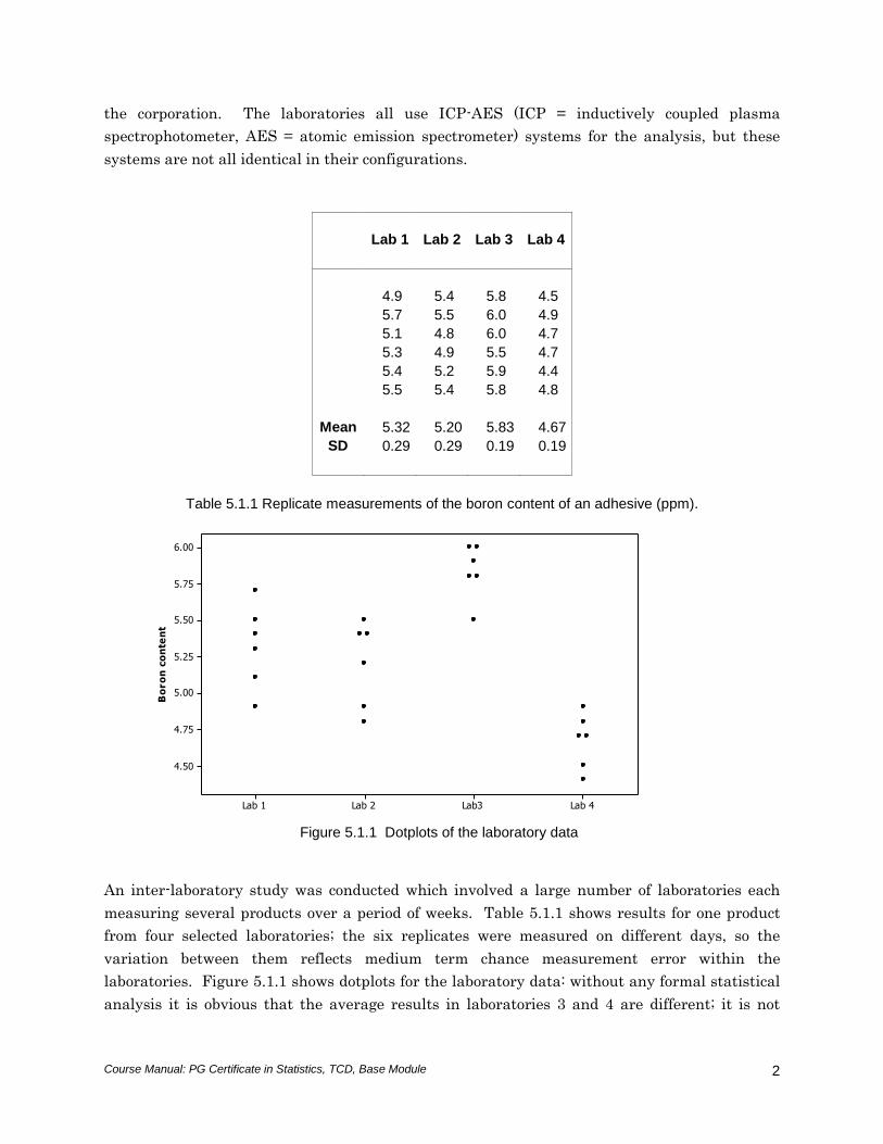
the corporation. The laboratories all use ICP-AES (ICP = inductively coupled plasma

spectrophotometer, AES = atomic emission spectrometer) systems for the analysis, but these

systems are not all identical in their configurations.

Lab 1 Lab 2 Lab 3 Lab 4

4.9 5.4 5.8 4.5

5.7 5.5 6.0 4.9

5.1 4.8 6.0 4.7

5.3 4.9 5.5 4.7

5.4 5.2 5.9 4.4

5.5 5.4 5.8 4.8

Mean 5.32 5.20 5.83 4.67

SD 0.29 0.29 0.19 0.19

Table 5.1.1 Replicate measurements of the boron content of an adhesive (ppm).

Lab 4Lab3Lab 2Lab 1

6.00

5.75

5.50

5.25

5.00

4.75

4.50

Bo

ro

n c

on

ten

t

Figure 5.1.1 Dotplots of the laboratory data

An inter-laboratory study was conducted which involved a large number of laboratories each

measuring several products over a period of weeks. Table 5.1.1 shows results for one product

from four selected laboratories; the six replicates were measured on different days, so the

variation between them reflects medium term chance measurement error within the

laboratories. Figure 5.1.1 shows dotplots for the laboratory data: without any formal statistical

analysis it is obvious that the average results in laboratories 3 and 4 are different; it is not


3

clear, however, whether laboratories 1 and 2 differ by more than the chance analytical day-to-

day variation which is clearly present in all laboratories.

Measuring variation

Variation between observations is usually measured by the standard deviation or, alternatively,

by its square, the variance. Thus, suppose we obtain a random sample of n observations,

nyyyy ,...,, 321 , from some population or process whose mean is μ and whose variance is σ2; the

sample variance (the square of the standard deviation) is defined as:

1

)(

1

2

2

n

yy

S

n

ii

. (5.1)

This quantity, which estimates the unknown σ2, is the average of the squared deviations of the

data, yi, from their overall mean, y , where the divisor is n–1, the ‘degrees of freedom’. The

term ‘degrees of freedom’ is used because only n–1 of the deviations )( yyi are free to vary:

they are constrained by the fact that they must sum to zero2. Thus, if n–1 deviations sum to

some arbitrary value, the last deviation is, necessarily, equal to minus that value.

When the data collection mechanism is more complicated than that assumed above, the method

known as Analysis of Variance (ANOVA) may be used to break up both the total sum of squares

(the numerator of 5.1) and the total degrees of freedom (the denominator of 5.1) into components

associated with the structure of the data collection process.

The basic idea underlying the simplest form of ANOVA is that the variation between individual

observations can be viewed as having two components: within-group and between-group. The

within-group component is seen as pure chance variation – within-group conditions are held

constant and there are no reasons why any two observations should be different, apart from the

influence of the chance variation that affects the system being studied. In the case of the

laboratories study, the same material was measured on each of six days using the same

equipment, the same glassware, the same reagents etc., by the same team of analysts, within

each laboratory. The key word here is ‘same’.

Between-group variation, on the other hand, is seen as (at least potentially) systematic:

different groups are different, or are treated differently, in ways that may lead to higher or

lower average responses. In the case of the laboratories, the equipment used was either

different (made by different manufacturers) or was set up in different ways; there were different

2 If this is not obvious, check that it is true for a simple example, say three values 6, 7, 8.


4

teams of analysts in the four laboratories, which were in different parts of the world with

markedly different climates. There were, as a result, many possible factors which could lead to

different average responses in the four laboratories.

ANOVA splits the variation, as measured by the corresponding sums of squares, into

components associated with these two categories (between and within-group) and then averages

the sums of squares, by dividing by the correspondingly partitioned degrees of freedom (see

below). This gives two mean squares, which correspond directly to expression (5.1) – they are

sample variances associated with within-group and between-group variation. If the between-

group mean square is not substantially bigger than the within-group mean square, which

measures purely chance variation, then there is no reason to believe that there are systematic

differences between the responses of the different groups. The statistical test for between-group

differences is based on the ratio of the two mean squares: MS(Between-group)/MS(Within-

group) – if this is large, it suggests systematic between-group differences.

We now turn our attention to the technical details.

Decomposing Sums of Squares

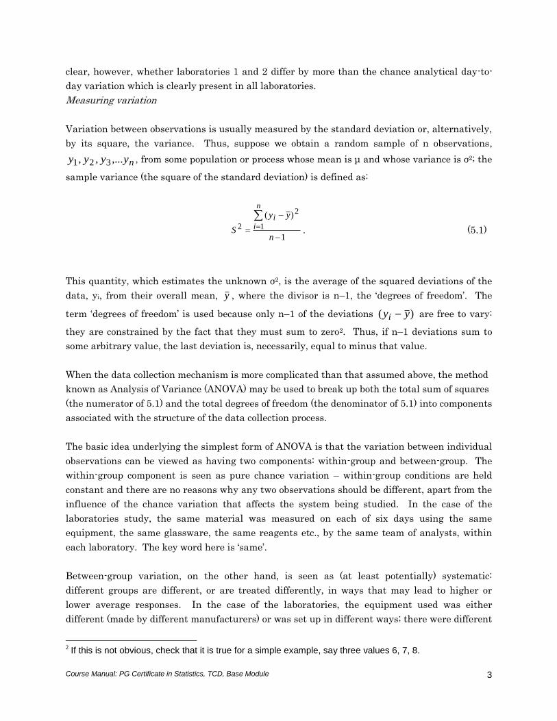
A slightly more elaborate notation, which reflects the within-group/between-group data

structure, is helpful when dealing with data from several groups. Thus, for the data of Table

5.1.1, each observation ijy is uniquely labelled by two subscripts: i refers to the group

(laboratory) in which the observation was generated (i=1,2,3,4) while j labels the replicates

within laboratory (j=1,2,..6). For example, y13=5.1 and y31=5.8 in Table 5.1.1. Figure 5.1.2 shows

schematically how the deviation of any observation ijy from the overall mean y can be

regarded as the sum of two components – its deviation from its own group mean3 ).( iyijy and

the deviation of its group mean from the overall mean ).( yiy . Thus we can write:

)()( .. yyyyyy iiijij . (5.2)

3 The mean of the six results in laboratory i is .iy ; the dot indicates that we have summed over the j sub-

script, the bar that we have averaged, i.e.,

6

16

1.

jiji yy . In general there are I groups and J replicates

within each group. It is not necessary that the number of replicates should be the same for each group, but adjustments to the calculations are required if this is not the case; the statistical software will take care of these.


5

Figure 5.1.2 The ANOVA decomposition

When both sides of equation (5.2) are squared and summed over all the data points, the cross-

product of the two terms on the right-hand side sums to zero and we get:

2.

2.

2 )()()( yyyyyy i

dataall

iij

dataall

ij

dataall

(5.3)

SS(total) = SS(within groups4) + SS(between groups) (5.4)

where SS stands for ‘sum of squares’.

For the laboratory study the decomposition of sums of squares is:

5.2996 = 1.1750 + 4.1246.

4 Note that statistics packages almost invariably refer to the component associated with purely random

variation as the ‘error’ component. In the current context this is the within-group component, so ‘within-group’ and ‘error’ sums of squares and degrees of freedom will be used interchangeably.

4321

6.0

5.5

5.0

4.5

Laboratory

Bo

ron

ijy

.iy

y.1y

.2y

.4y

.iij yy

yy i .

The within-group deviation

The between-group deviation


6

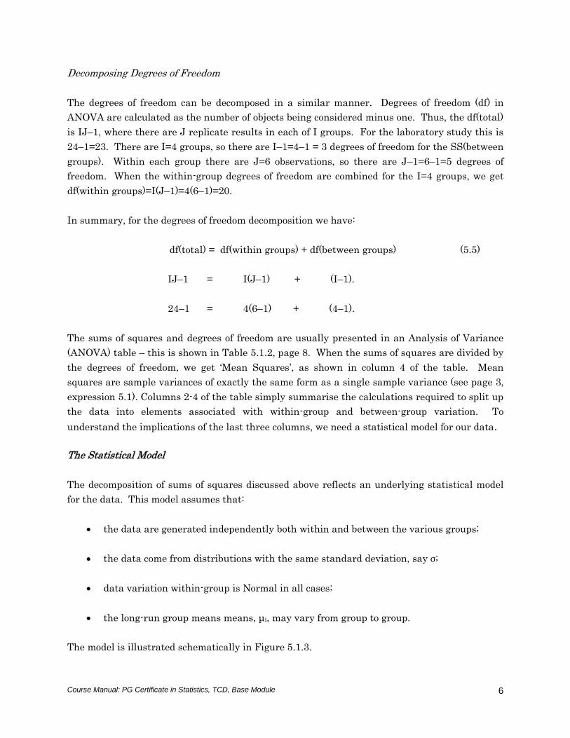
Decomposing Degrees of Freedom

The degrees of freedom can be decomposed in a similar manner. Degrees of freedom (df) in

ANOVA are calculated as the number of objects being considered minus one. Thus, the df(total)

is IJ–1, where there are J replicate results in each of I groups. For the laboratory study this is

24–1=23. There are I=4 groups, so there are I–1=4–1 = 3 degrees of freedom for the SS(between

groups). Within each group there are J=6 observations, so there are J–1=6–1=5 degrees of

freedom. When the within-group degrees of freedom are combined for the I=4 groups, we get

df(within groups)=I(J–1)=4(6–1)=20.

In summary, for the degrees of freedom decomposition we have:

df(total) = df(within groups) + df(between groups) (5.5)

IJ–1 = I(J–1) + (I–1).

24–1 = 4(6–1) + (4–1).

The sums of squares and degrees of freedom are usually presented in an Analysis of Variance

(ANOVA) table – this is shown in Table 5.1.2, page 8. When the sums of squares are divided by

the degrees of freedom, we get ‘Mean Squares’, as shown in column 4 of the table. Mean

squares are sample variances of exactly the same form as a single sample variance (see page 3,

expression 5.1). Columns 2-4 of the table simply summarise the calculations required to split up

the data into elements associated with within-group and between-group variation. To

understand the implications of the last three columns, we need a statistical model for our data.

The Statistical Model

The decomposition of sums of squares discussed above reflects an underlying statistical model

for the data. This model assumes that:

the data are generated independently both within and between the various groups;

the data come from distributions with the same standard deviation, say σ;

data variation within-group is Normal in all cases;

the long-run group means means, μi, may vary from group to group.

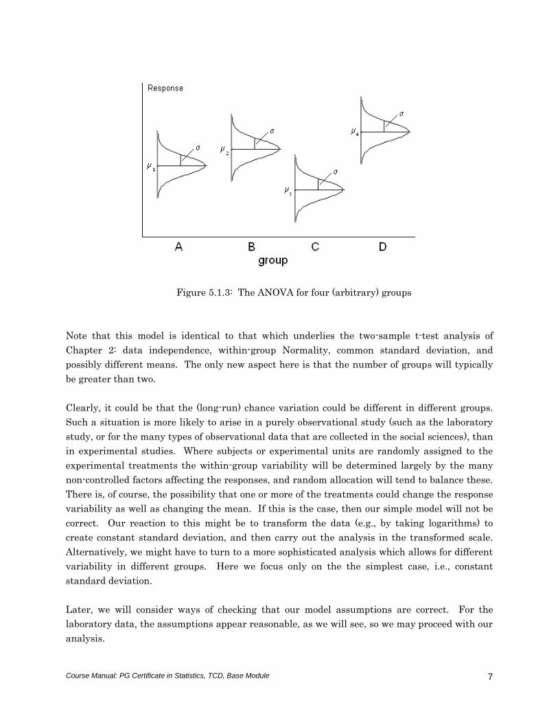
The model is illustrated schematically in Figure 5.1.3.


7

Figure 5.1.3: The ANOVA for four (arbitrary) groups

Note that this model is identical to that which underlies the two-sample t-test analysis of

Chapter 2: data independence, within-group Normality, common standard deviation, and

possibly different means. The only new aspect here is that the number of groups will typically

be greater than two.

Clearly, it could be that the (long-run) chance variation could be different in different groups.

Such a situation is more likely to arise in a purely observational study (such as the laboratory

study, or for the many types of observational data that are collected in the social sciences), than

in experimental studies. Where subjects or experimental units are randomly assigned to the

experimental treatments the within-group variability will be determined largely by the many

non-controlled factors affecting the responses, and random allocation will tend to balance these.

There is, of course, the possibility that one or more of the treatments could change the response

variability as well as changing the mean. If this is the case, then our simple model will not be

correct. Our reaction to this might be to transform the data (e.g., by taking logarithms) to

create constant standard deviation, and then carry out the analysis in the transformed scale.

Alternatively, we might have to turn to a more sophisticated analysis which allows for different

variability in different groups. Here we focus only on the the simplest case, i.e., constant

standard deviation.

Later, we will consider ways of checking that our model assumptions are correct. For the

laboratory data, the assumptions appear reasonable, as we will see, so we may proceed with our

analysis.


8

The ANOVA Table

Source of Sums of Degrees of Mean Expected

Variation Squares Freedom Squares Mean Squares F-value p-value

Between

groups 4.1246 3 1.3749

1

)(1

2

2

IJ

I

ii

23.40 <0.0005

Within-

groups or

Error

1.1750 20

0.0588 2

Total 5.2996 23

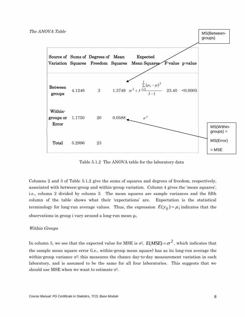
Table 5.1.2 The ANOVA table for the laboratory data

Columns 2 and 3 of Table 5.1.2 give the sums of squares and degrees of freedom, respectively,

associated with between-group and within-group variation. Column 4 gives the ‘mean squares’,

i.e., column 2 divided by column 3. The mean squares are sample variances and the fifth

column of the table shows what their ‘expectations’ are. Expectation is the statistical

terminology for long-run average values. Thus, the expression iijyE )( indicates that the

observations in group i vary around a long-run mean μi.

Within Groups

In column 5, we see that the expected value for MSE is σ2, 2)( MSEE , which indicates that

the sample mean square error (i.e., within-group mean square) has as its long-run average the

within-group variance σ2; this measures the chance day-to-day measurement variation in each

laboratory, and is assumed to be the same for all four laboratories. This suggests that we

should use MSE when we want to estimate σ2.

MS(Between-groups)

MS(Within-groups) = MS(Error) = MSE


9

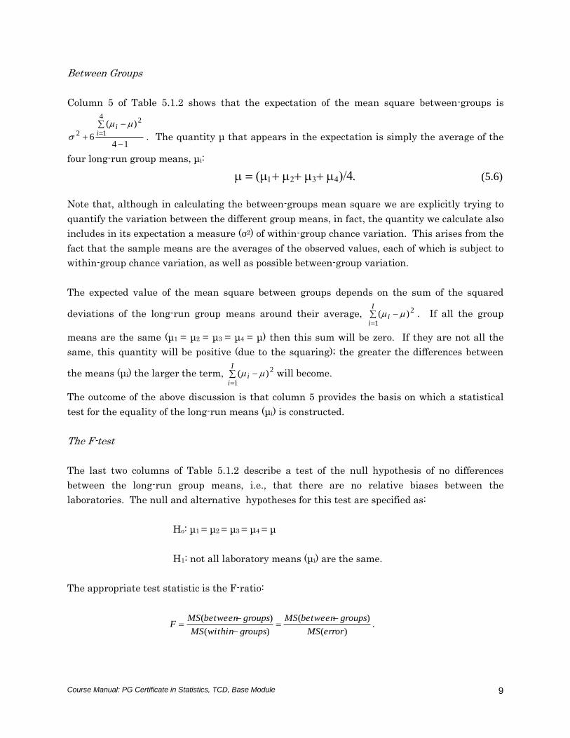
Between Groups

Column 5 of Table 5.1.2 shows that the expectation of the mean square between-groups is

14

)(

6

4

1

2

2

ii

. The quantity μ that appears in the expectation is simply the average of the

four long-run group means, μi:

(5.6)

Note that, although in calculating the between-groups mean square we are explicitly trying to

quantify the variation between the different group means, in fact, the quantity we calculate also

includes in its expectation a measure (σ2) of within-group chance variation. This arises from the

fact that the sample means are the averages of the observed values, each of which is subject to

within-group chance variation, as well as possible between-group variation.

The expected value of the mean square between groups depends on the sum of the squared

deviations of the long-run group means around their average,

I

ii

1

2)( . If all the group

means are the same (μ1 = μ2 = μ3 = μ4 = μ) then this sum will be zero. If they are not all the

same, this quantity will be positive (due to the squaring); the greater the differences between

the means (μi) the larger the term,

I

ii

1

2)( will become.

The outcome of the above discussion is that column 5 provides the basis on which a statistical

test for the equality of the long-run means (μi) is constructed.

The F-test

The last two columns of Table 5.1.2 describe a test of the null hypothesis of no differences

between the long-run group means, i.e., that there are no relative biases between the

laboratories. The null and alternative hypotheses for this test are specified as:

Ho: μ1 = μ2 = μ3 = μ4 = μ

H1: not all laboratory means (μi) are the same.

The appropriate test statistic is the F-ratio:

)(

)(

)(

)(

errorMS

groupsbetweenMS

groupswithinMS

groupsbetweenMSF

.


10

If the null hypothesis is true, then both the numerator and denominator of the F-ratio have the

same expectation, σ2, (since all the deviation μi – μ) terms are zero when the null hypothesis is

true) and the ratio should be about one.

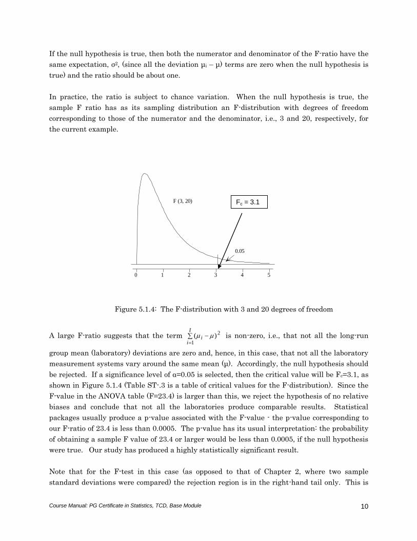
In practice, the ratio is subject to chance variation. When the null hypothesis is true, the

sample F ratio has as its sampling distribution an F-distribution with degrees of freedom

corresponding to those of the numerator and the denominator, i.e., 3 and 20, respectively, for

the current example.

Figure 5.1.4: The F-distribution with 3 and 20 degrees of freedom

A large F-ratio suggests that the term

I

ii

1

2)( is non-zero, i.e., that not all the long-run

group mean (laboratory) deviations are zero and, hence, in this case, that not all the laboratory

measurement systems vary around the same mean (μ). Accordingly, the null hypothesis should

be rejected. If a significance level of α=0.05 is selected, then the critical value will be Fc=3.1, as

shown in Figure 5.1.4 (Table ST-.3 is a table of critical values for the F-distribution). Since the

F-value in the ANOVA table (F=23.4) is larger than this, we reject the hypothesis of no relative

biases and conclude that not all the laboratories produce comparable results. Statistical

packages usually produce a p-value associated with the F-value - the p-value corresponding to

our F-ratio of 23.4 is less than 0.0005. The p-value has its usual interpretation: the probability

of obtaining a sample F value of 23.4 or larger would be less than 0.0005, if the null hypothesis

were true. Our study has produced a highly statistically significant result.

Note that for the F-test in this case (as opposed to that of Chapter 2, where two sample

standard deviations were compared) the rejection region is in the right-hand tail only. This is

543210

F (3, 20)

0.05

Fc = 3.1


11

so because the

I

ii

1

2)( terms are squared in the expression for the between-groups expected

mean square; hence, the numerator of the F statistic is expected to be bigger than the

denominator and the F-ratio is expected to be bigger than 1, when there are differences between

the groups. A small value of F would be regarded a purely chance event.

Note that the sample size is the same for each group in this and all the other examples of the

chapter. This is purely for simplicity of presentation – the calculations are a bit messier if the

number of observations changes from group to group, but conceptually nothing changes.

Suitable software (such as Minitab) allows for this. In multi-factor designs, where different

sized groups of subjects or experimental units are studied, the non-constant sample size can

cause problems. Such issues are, however, outside the scope of the current discussion.

Model validation

The F-test has established that not all the laboratory means are the same, but we still need to

establish which ones are different and by how much they differ from each other. Before doing

this, we will turn our attention to checking that the assumptions underlying the analysis are

valid. If they are valid, then it makes sense to carry on to a more detailed examination of the

data. If they are not valid, then the F-test may not be valid and the conclusions drawn from it

will be suspect. The validation is based on the analysis of residuals, as was the case for two-

sample t-tests.

When the laboratory means (the fitted values) are subtracted from the corresponding data

points within each laboratory, we are left with the residuals – by construction these vary about

a mean of zero. If our model assumptions of Normality and constant within-laboratory standard

deviation are correct, these residuals should have the properties that would be expected from

four random samples from a single Normal distribution, with zero mean.

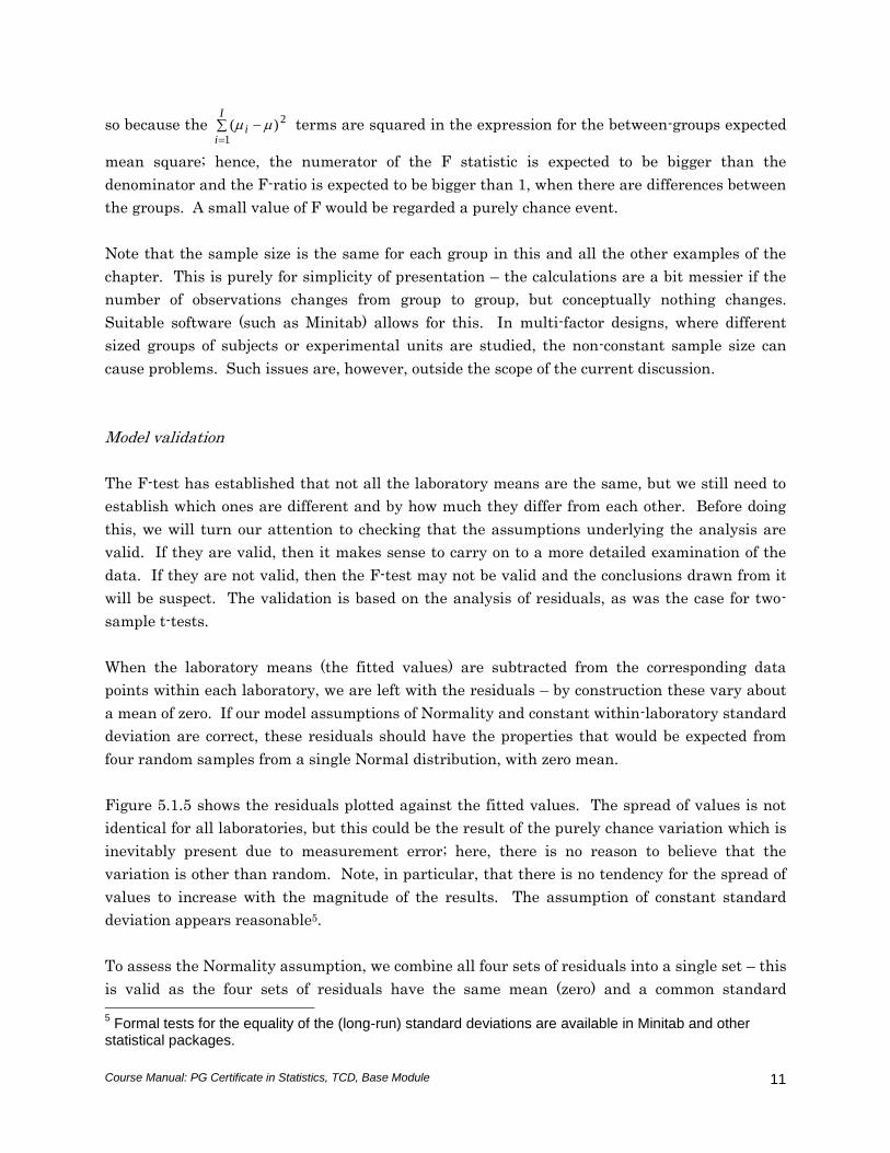
Figure 5.1.5 shows the residuals plotted against the fitted values. The spread of values is not

identical for all laboratories, but this could be the result of the purely chance variation which is

inevitably present due to measurement error; here, there is no reason to believe that the

variation is other than random. Note, in particular, that there is no tendency for the spread of

values to increase with the magnitude of the results. The assumption of constant standard

deviation appears reasonable5.

To assess the Normality assumption, we combine all four sets of residuals into a single set – this

is valid as the four sets of residuals have the same mean (zero) and a common standard 5 Formal tests for the equality of the (long-run) standard deviations are available in Minitab and other

statistical packages.


12

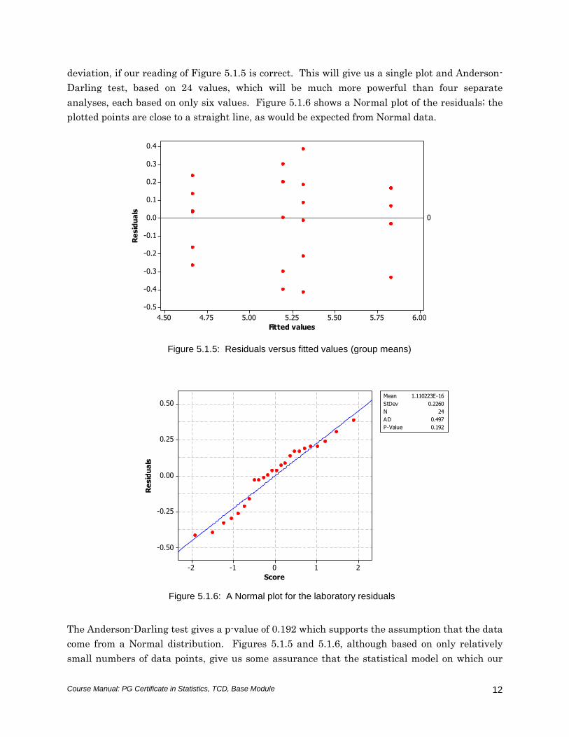
deviation, if our reading of Figure 5.1.5 is correct. This will give us a single plot and Anderson-

Darling test, based on 24 values, which will be much more powerful than four separate

analyses, each based on only six values. Figure 5.1.6 shows a Normal plot of the residuals; the

plotted points are close to a straight line, as would be expected from Normal data.

6.005.755.505.255.004.754.50

0.4

0.3

0.2

0.1

0.0

-0.1

-0.2

-0.3

-0.4

-0.5

Fitted values

Re

sid

ua

ls

0

Figure 5.1.5: Residuals versus fitted values (group means)

0.50

0.25

0.00

-0.25

-0.50

210-1-2

Re

sid

ua

ls

Score

Mean 1.110223E-16

StDev 0.2260

N 24

AD 0.497

P-Value 0.192

Figure 5.1.6: A Normal plot for the laboratory residuals

The Anderson-Darling test gives a p-value of 0.192 which supports the assumption that the data

come from a Normal distribution. Figures 5.1.5 and 5.1.6, although based on only relatively

small numbers of data points, give us some assurance that the statistical model on which our


13

ANOVA F-test was based is acceptable. The same assumptions are required for the tests and

confidence intervals discussed next.

Comparing Means - Least Significant Difference

From this point on in the notes we change our notation slightly and adopt 𝑰 to label the number of

observations (i.e. rows in the data table) while 𝑱 is used to label the number of columns (i.e. groups) in our

data table; this notation is more in keeping with standard mathematical notation.

The F-test is a global test that asks if all the long-run group means are the same or not. Once,

as here, the F-test indicates that differences exist, we need to carry out some further analysis to

investigate the pattern of differences. A natural approach to comparing any pair of sample

means is to carry out a t-test of the hypothesis that their long-run values do not differ. We saw

in Chapter 2 that the difference between any pair of means jy and ky (i.e. the mean of column

𝑗 and mean of a different column 𝑘 in our data table) is statistically significant if:

c

kjt

n

s

yyt

22

that is if

n

styy ckj

22 (5.7)

where the sample size is n in each case, s2 is the combined within-group variance, tc is the

critical value for a two-sided test with a significance level of α=0.05, and jy > ky . Thus, the

quantity on the R.H.S. of (5.7) is the ‘least significant difference’ (LSD) – the smallest difference

between two sample means that will be declared statistically significant.

For our laboratory comparison study we have four means, each based on J=6 observations. We

have a combined within-laboratory variance of s2=MSE=0.0588, which is based on all 𝐽 = 4

laboratories. We use this as our estimate of σ2; thus, when we compare two means, say for labs

1 and 2, we ‘borrow’ degrees of freedom from the other laboratories. The degrees of freedom for

the t-distribution used to determine the critical values for the t-test are the same as those for

s2=MSE, and so they are 20 in this case. Thus, by using MSE6, rather than 𝑠2 = (𝑠12 + 𝑠2

2)/2

(based on the two laboratories being compared), we gain an extra 10 degrees of freedom for the

test and it becomes, accordingly, more powerful.

6 In fact, MSE is just the average of the four sample variances: MSE

ssssS

4

24

23

22

212


14

As stated above, the quantity on the right-hand side of expression (5.7) is the smallest

difference between two sample means which will lead us to conclude that the corresponding

population means should be considered different. Note that since σ2 is assumed the same for all

groups and each mean is based on J=6 observations, the LSD applies to all possible comparisons

between pairs of means, not just to laboratories 1 and 2. Here we have:

Least Significant Difference (LSD) = I

MSEtc

2=

6

)0588.0(209.2 = 0.29. (5.8)

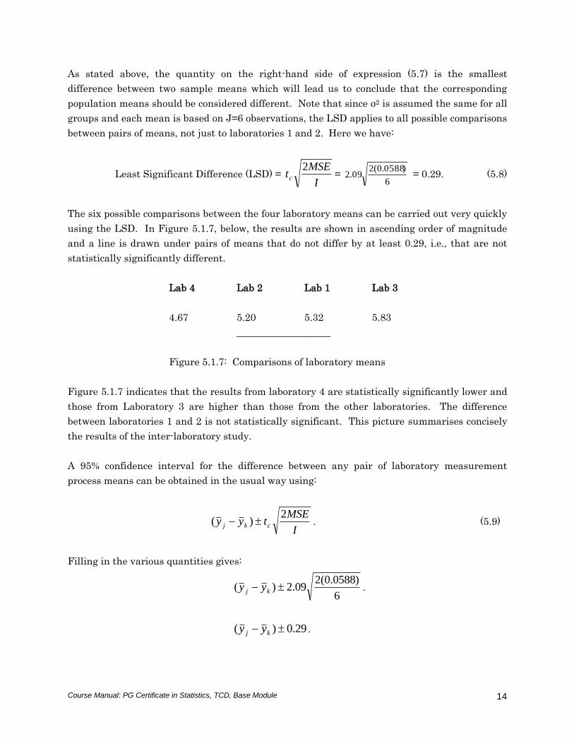
The six possible comparisons between the four laboratory means can be carried out very quickly

using the LSD. In Figure 5.1.7, below, the results are shown in ascending order of magnitude

and a line is drawn under pairs of means that do not differ by at least 0.29, i.e., that are not

statistically significantly different.


4.67 5.20 5.32 5.83

___________________

Figure 5.1.7: Comparisons of laboratory means

Figure 5.1.7 indicates that the results from laboratory 4 are statistically significantly lower and

those from Laboratory 3 are higher than those from the other laboratories. The difference

between laboratories 1 and 2 is not statistically significant. This picture summarises concisely

the results of the inter-laboratory study.

A 95% confidence interval for the difference between any pair of laboratory measurement

process means can be obtained in the usual way using:

I

MSEtyy ckj

2)( . (5.9)

Filling in the various quantities gives:

6

)0588.0(209.2)( kj yy .

29.0)( kj yy .


15

Thus, the error bounds on any difference kj yy are obtained by adding and subtracting 0.29

from the calculated difference. The confidence interval measures the relative bias between the

two laboratories.

Multiple Comparisons

Our investigation of the pattern of differences between the laboratory means essentially

involves carrying out six t-tests: we can select six pairs from four groups. The number of

possible comparisons grows rapidly with the number of groups involved. Thus, comparing the

means for six groups involves 152.1

5.6 pairs of means, while ten groups would allow 45

2.1

9.10

comparisons to be made. Multiple comparisons present us with a difficulty: the statistical

properties of t-tests, as discussed in Chapters 2 and 4, hold for a single test, but will change

radically if many tests are carried out simultaneously. This is very often ignored when only a

small number of tests are carried out, but it becomes increasingly important when many

comparisons are made. To see where the problem lies, we note that for any one test the

significance level is the probability of rejecting the hypothesis of no difference between the long-

run means, when, in fact, there is no difference, i.e., when the null hypothesis is true. However,

the probability is much higher than, say, α=0.05 that one or more of the six comparisons for the

laboratory study will produce a statistically significant result, when in fact there are no

systematic differences.

To understand why this is so, consider a simple coin tossing experiment. If a fair coin is tossed,

the probability of the result being a head is 1/2. However, the probability of one or more heads

in six tosses is considerably higher. Thus, the probability that all six results are tails is

(1/2)6=1/64, so that the probability of at least one head is 1–(1/2)6=63/64. The corresponding

calculation for the comparisons between the laboratories cannot be carried out in this simple

way (since the comparisons involving pairs of means are not all independent of each other, as

was assumed for the coin tossing experiment) but the underlying ideas are the same. However,

the analogy suggests that use of multiple statistical tests simultaneously can lead to much

higher Type 1 error rates than the individual significance levels would suggest. Type 1 error

occurs when we “see” or detect an effect (i.e. a significant difference) when actually there is

none. In this situation we falsely reject the null hypothesis of equal group means when in fact

the group means are equal – ideally this situation should be avoided.


16

Aside:

Let us consider this situation in a little more detail. If, for argument sake we take it that

H0 is in fact true and we set α=0.05, then in 95% of cases where we test H0 we will not

reject (i.e. accept) H0 – clearly this is the outcome we want “accept H0 when it is true”.

But of course we’ll also reject H0 in 5% of cases when H0 is actually true, so we make a

Type 1 error 5% of the time. Thus, if we set α=0.05 then this also specifies the

probability of making a Type 1 error. Interestingly, we can also express this probability

α as follows:

𝛼 = 1 − (1 − 𝛼)

Clearly the quantity (1-α) in this equation is the probability of accepting H0 when it is

true – the complementary event. Taking this a step further, if we test two independent

null hypothesis when both are true, then the probability of making at least one Type 1

error is obviously 1 – probability of making no Type 1 errors, or

𝑃 (𝑜𝑛𝑒 𝑇𝑦𝑝𝑒 1 𝑒𝑟𝑟𝑜𝑟 𝑖𝑛 2 𝑡𝑒𝑠𝑡𝑠 𝑜𝑓 𝐻0) = 1 − (1 − 𝛼) × (1 − 𝛼)

since, (1 − 𝛼) × (1 − 𝛼) is the probability of no (i.e. 0) Type 1 errors being made on the

first test of H0 based on a sample from the population, followed by a second separate test

of H0 using a different sample of data taken from the same population. More generally, if

we make 𝑚 pairwise comparisons of the data the probability of making at least one Type

1 error is:

𝑃 (𝑜𝑛𝑒 𝑇𝑦𝑝𝑒 1 𝑒𝑟𝑟𝑜𝑟 𝑖𝑛 𝑚 𝑡𝑒𝑠𝑡𝑠 𝑜𝑓 𝐻0) = 1 − (1 − 𝛼)𝑚

Thus for the lab data with α=0.05 and where we have 6 comparisons the probability of

making at least one Type 1 error is

𝑃 (𝑜𝑛𝑒 𝑇𝑦𝑝𝑒 1 𝑒𝑟𝑟𝑜𝑟 𝑖𝑛 6 𝑡𝑒𝑠𝑡𝑠 𝑜𝑓 𝐻0) = 1 − (1 − 𝛼)6 = 1 − 0.956 = 1 − 0.74 = 0.26

This gives a true multiple comparison value for α that is over 5 times the so-called

‘nominal’ value set for α=0.05. Importantly, this means that if we want to get α=0.05

level of significance for a single pairwise comparison having already assumed a 5% level

for our ANOVA tests we should adjust our α=0.05/5 = 0.01.

Note that the LSD method discussed above makes no allowance for the fact that

multiple tests are being carried out (or, equivalently, multiple simultaneous confidence

intervals are being calculated) on the same data. For this reason, I do not recommend

the use of LSD for the analysis of real data.


17

Interestingly, if we were conducting 𝑚 = 20 pairwise tests the probability is 0.64 or 13

times the nominal value of α = 0.05, requiring an adjustment of α = 0.05/13 = 0.004.

Meanwhile, for 45 tests we have a Type 1 probability of 0.9 and would require α =

0.05/18 = 0.003, which is quite small in practice and is too conservative – a more

practical value as 𝑚 gets big is α/J, for J groups.

Various strategies are adopted to deal with the multiple comparison problem, but they all

involve making the individual tests less powerful, i.e., less likely to detect a small but real

difference between the means. One simple approach is to reduce the significance level of the

individual tests (say to α=0.01), so that the error rate for the family of comparisons is reduced to

a more acceptable level. Minitab offers other multiple comparison alternatives (see Appendix).

Bonferroni Corrected (1 - α) x 100% Confidence Intervals for pair-wise comparisons of group

means within ANOVA

One well known strategy for dealing with multiple comparisons is to apply the so-called

Bonferroni Confidence Interval. If we have say 𝑚 simple comparisons, each with an α level of

significance, then we should expect that the combined significance level will be 𝑚 × 𝛼.

Accordingly, if we have a multiple comparison where we specify the combined significance level

α, then any single pair-wise comparison test from among the set of 𝑚 pair-wise comparison

tests should have a significance level of 𝛼/𝑚. This gives rise to the so-called Bonferroni

corrected confidence intervals. For any pair of selected group means labelled �̅�𝑖 𝑎𝑛𝑑 �̅�𝑗 the two-

sided Bonferroni corrected confidence interval (based on a two-sided t-test tables) is given by

�̅�𝑗 − �̅�𝑘 = 𝑡𝑛1+𝑛2−𝐼 (𝛼

𝑚) √

𝑠2

𝑛1+

𝑠2

𝑛2

where 𝑠 is the overall pooled standard deviation across all 𝐽 groups combined7. Specifically,

when the samples sizes in each group are the same and equal to 𝐼 units in each group then we

get

�̅�𝑗 − �̅�𝑘 = 𝑡𝐼𝐽−𝐽 (𝛼

𝑚) √

2𝑠2

𝐼= 𝑡𝐼𝐽−𝐽 (

𝛼

𝑚) √

2 × 𝑀𝑆𝐸

𝐼

However, the value 𝑚 for the number of comparisons tests based on 𝐽 groups is problematic

when 𝐽 ≥ 7. Form above we have

𝑚 = (𝐽2

) =𝐽(𝐽 − 1)

2

7 Note: Where the statistical tables display one-side probability values then the adjustment to α should be α/2m and

not α/m as given here for the statistical table ST-2.


18

So if the number of groups 𝐽 gets large the, say 10) then 𝑚 = 45 and therefore 𝛼

𝑚=

0.05

45= 0.001,

this value is very small indeed and a t-crit value for the pairwise statistical test based on it

tends to reject the null hypothesis too often. In fact in this example the Bonferroni adjusted α

would suggest there is just a 1-in-a-1,000 chance of rejecting the null hypothesis. In practice

this is often too small and it makes more sense approximate 𝛼

𝑚 by

𝛼

𝐽. Using this value our

comparison formula becomes

�̅�𝑗 − �̅�𝑘 = 𝑡𝐼𝐽−𝐽 (𝛼

𝑚) √

2 × 𝑀𝑆𝐸

𝐼≈ 𝑡𝐼𝐽−𝐽 (

𝛼

𝐼) √

2 × 𝑀𝑆𝐸

𝐼

For a single pairwise t-test of the lab comparison data to be consistent with the earlier ANOVA

tests we have 𝑚 =𝐽(𝐽−1)

2=

4(4−1)

2= 6 and adjust our significance level to

𝛼

𝑚=

0.05

6

�̅�𝑘 − �̅�𝑘 = 𝑡4×6−4 (0.05

6) √

2 × 𝑀𝑆𝐸

𝐼= 𝑡20(0.008)√

2 × 0.0588

6

�̅�𝑗 − �̅�𝑘 = 2.99√2 × 0.0588

6= 0.419 ≈ 0.42

This interval is 1/3rd wider than the LSD interval computed above, accordingly it is less likely to

find a significant difference in a pairwise comparison of several group means.

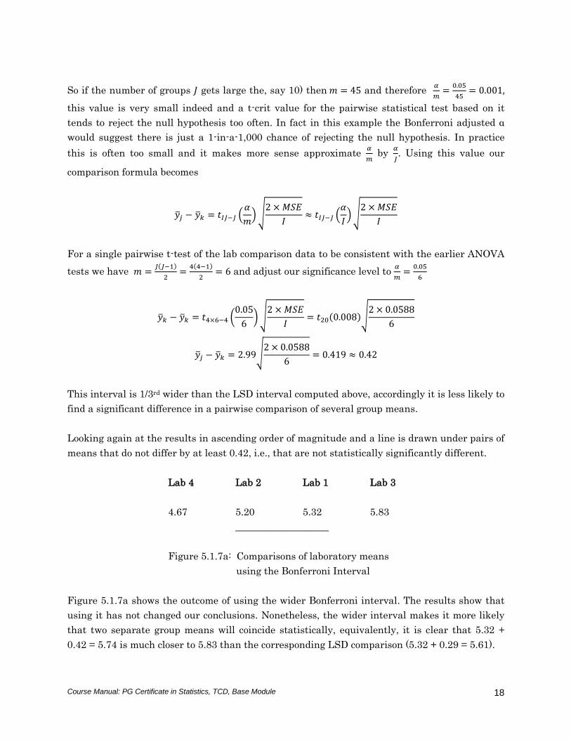
Looking again at the results in ascending order of magnitude and a line is drawn under pairs of

means that do not differ by at least 0.42, i.e., that are not statistically significantly different.


4.67 5.20 5.32 5.83

___________________

Figure 5.1.7a: Comparisons of laboratory means

using the Bonferroni Interval

Figure 5.1.7a shows the outcome of using the wider Bonferroni interval. The results show that

using it has not changed our conclusions. Nonetheless, the wider interval makes it more likely

that two separate group means will coincide statistically, equivalently, it is clear that 5.32 +

0.42 = 5.74 is much closer to 5.83 than the corresponding LSD comparison (5.32 + 0.29 = 5.61).


19

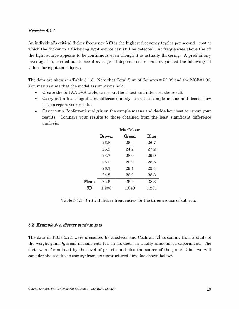
Exercise 5.1.1

An individual’s critical flicker frequency (cff) is the highest frequency (cycles per second - cps) at

which the flicker in a flickering light source can still be detected. At frequencies above the cff

the light source appears to be continuous even though it is actually flickering. A preliminary

investigation, carried out to see if average cff depends on iris colour, yielded the following cff

values for eighteen subjects.

The data are shown in Table 5.1.3. Note that Total Sum of Squares = 52.08 and the MSE=1.96.

You may assume that the model assumptions hold.

Create the full ANOVA table, carry out the F-test and interpret the result.

Carry out a least significant difference analysis on the sample means and decide how

best to report your results.

Carry out a Bonferroni analysis on the sample means and decide how best to report your

results. Compare your results to those obtained from the least significant difference

analysis.

Iris Colour

Brown Green Blue

26.8 26.4 26.7

26.9 24.2 27.2

23.7 28.0 29.9

25.0 26.9 28.5

26.3 29.1 29.4

24.8 26.9 28.3

Mean 25.6 26.9 28.3

SD 1.283 1.649 1.231

Table 5.1.3: Critical flicker frequencies for the three groups of subjects

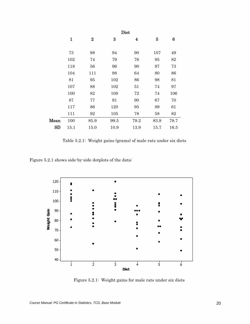
5.2 Example 2: A dietary study in rats

The data in Table 5.2.1 were presented by Snedecor and Cochran [2] as coming from a study of

the weight gains (grams) in male rats fed on six diets, in a fully randomised experiment. The

diets were formulated by the level of protein and also the source of the protein; but we will

consider the results as coming from six unstructured diets (as shown below).


20

Diet

1 2 3 4 5 6

73 98 94 90 107 49

102 74 79 76 95 82

118 56 96 90 97 73

104 111 98 64 80 86

81 95 102 86 98 81

107 88 102 51 74 97

100 82 108 72 74 106

87 77 91 90 67 70

117 86 120 95 89 61

111 92 105 78 58 82

Mean 100 85.9 99.5 79.2 83.9 78.7

SD 15.1 15.0 10.9 13.9 15.7 16.5

Table 5.2.1: Weight gains (grams) of male rats under six diets

Figure 5.2.1 shows side-by-side dotplots of the data:

654321

120

110

100

90

80

70

60

50

40

Diet

We

igh

t G

ain

Figure 5.2.1: Weight gains for male rats under six diets


21

The picture suggests that diets 1 and 3 may result in higher weight gains than the other diets,

but given the chance variation within the six groups, it is as well to check this out with formal

statistical tests. Also, it is not clear whether or not there are differences between the other

diets.

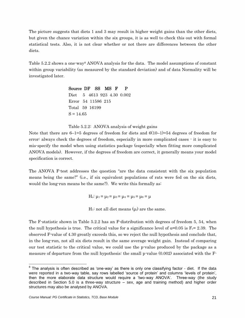
Table 5.2.2 shows a one-way8 ANOVA analysis for the data. The model assumptions of constant

within group variability (as measured by the standard deviation) and of data Normality will be

investigated later.

Source DF SS MS F P

Diet 5 4613 923 4.30 0.002

Error 54 11586 215

Total 59 16199

S = 14.65

Table 5.2.2: ANOVA analysis of weight gains

Note that there are 6–1=5 degrees of freedom for diets and 6(10–1)=54 degrees of freedom for

error: always check the degrees of freedom, especially in more complicated cases - it is easy to

mis-specify the model when using statistics package (especially when fitting more complicated

ANOVA models). However, if the degrees of freedom are correct, it generally means your model

specification is correct.

The ANOVA F-test addresses the question “are the data consistent with the six population

means being the same?” (i.e., if six equivalent populations of rats were fed on the six diets,

would the long-run means be the same?). We write this formally as:

Ho: μ1 = μ2 = μ3 = μ4 = μ5 = μ6 = μ

H1: not all diet means (μi) are the same.

The F-statistic shown in Table 5.2.2 has an F-distribution with degrees of freedom 5, 54, when

the null hypothesis is true. The critical value for a significance level of α=0.05 is Fc= 2.39. The

observed F-value of 4.30 greatly exceeds this, so we reject the null hypothesis and conclude that,

in the long-run, not all six diets result in the same average weight gain. Instead of comparing

our test statistic to the critical value, we could use the p-value produced by the package as a

measure of departure from the null hypothesis: the small p-value (0.002) associated with the F-

8 The analysis is often described as ‘one-way’ as there is only one classifying factor - diet. If the data

were reported in a two-way table, say rows labelled ‘source of protein’ and columns ‘levels of protein’, then the more elaborate data structure would require a ‘two-way ANOVA’. Three-way (the study described in Section 5.0 is a three-way structure – sex, age and training method) and higher order structures may also be analysed by ANOVA.


22

test makes such an hypothesis implausible – at least one of the diets is likely to produce weight

gains that show a different mean to the others.

Model Validation

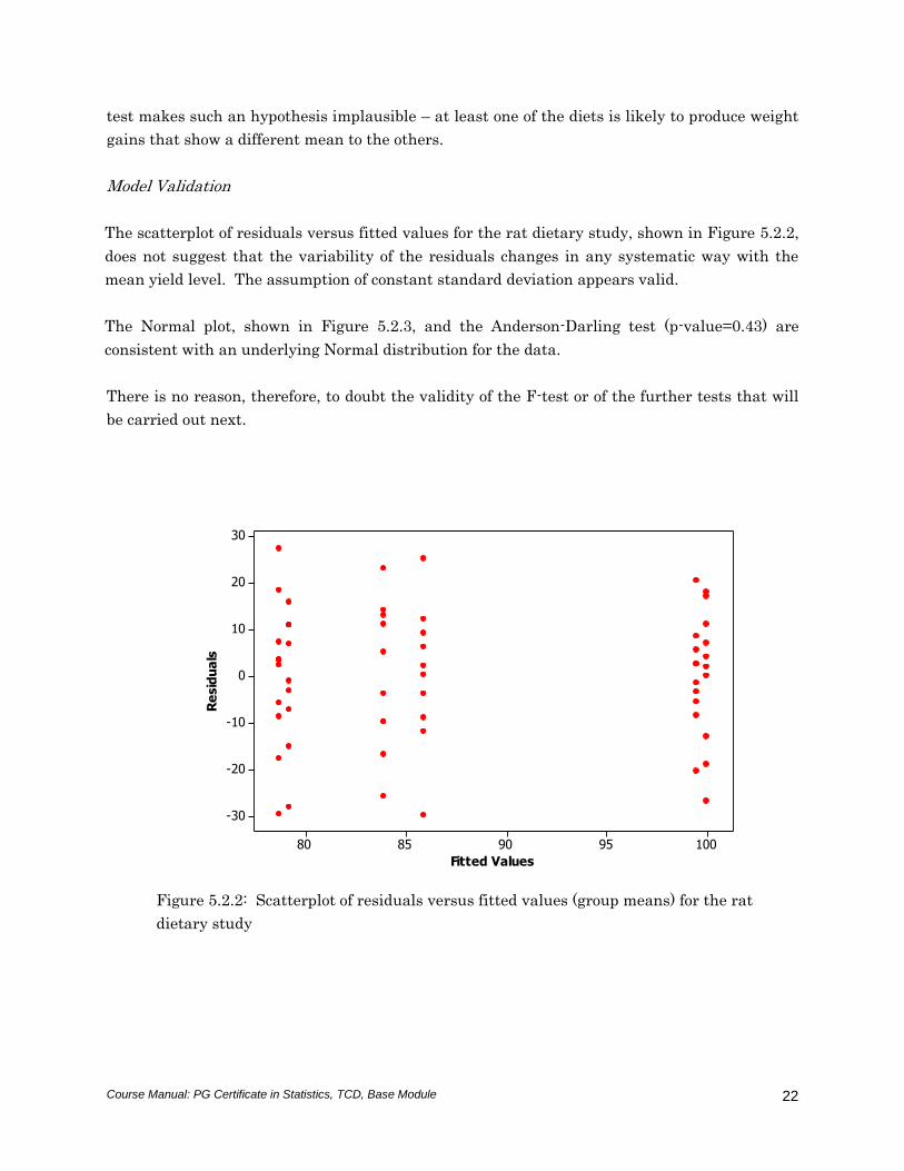
The scatterplot of residuals versus fitted values for the rat dietary study, shown in Figure 5.2.2,

does not suggest that the variability of the residuals changes in any systematic way with the

mean yield level. The assumption of constant standard deviation appears valid.

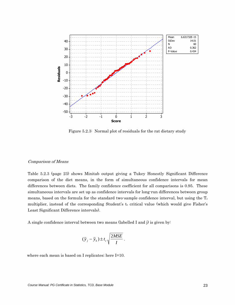
The Normal plot, shown in Figure 5.2.3, and the Anderson-Darling test (p-value=0.43) are

consistent with an underlying Normal distribution for the data.

There is no reason, therefore, to doubt the validity of the F-test or of the further tests that will

be carried out next.

10095908580

30

20

10

0

-10

-20

-30

Fitted Values

Re

sid

ua

ls

Figure 5.2.2: Scatterplot of residuals versus fitted values (group means) for the rat

dietary study


23

40

30

20

10

0

-10

-20

-30

-40

-50

3210-1-2-3

Re

sid

ua

ls

Score

Mean 6.631732E-15

StDev 14.01

N 60

AD 0.362

P-Value 0.434

Figure 5.2.3: Normal plot of residuals for the rat dietary study

Comparison of Means

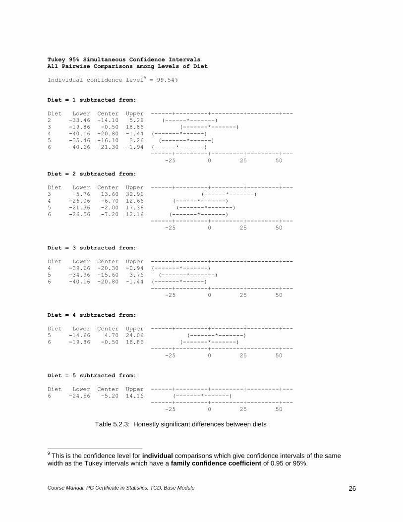
Table 5.2.3 (page 23) shows Minitab output giving a Tukey Honestly Significant Difference

comparison of the diet means, in the form of simultaneous confidence intervals for mean

differences between diets. The family confidence coefficient for all comparisons is 0.95. These

simultaneous intervals are set up as confidence intervals for long-run differences between group

means, based on the formula for the standard two-sample confidence interval, but using the Tc

multiplier, instead of the corresponding Student’s tc critical value (which would give Fisher’s

Least Significant Difference intervals).

A single confidence interval between two means (labelled I and j) is given by:

I

MSEtyy ckj

2)( .

where each mean is based on I replicates; here I=10.


24

To get the simultaneous Tukey intervals, we replace the t-multiplier by:

))1(,,1(2

1 IJJqTc

where J = 6 is the number of means to be compared and I =10 is the number of replicates in

each group. Our Table ST-6 does not give Studentised Ranges (q) with degrees of freedom ν=54;

we will use instead the nearest value q(6,60) = 4.16 [the value for ν=54 is, in fact, 4.17]. The

corresponding Tc value is found by multiplying by 1/2: for degrees of freedom ν=60 we get:

94.2)16.4(2

1)60,6,95.0(

2

1))1(,,1(

2

1 qIJJqTc .

The estimated standard error of the difference between two means is:

56.610

)215(22

I

MSE

which, when multiplied by the Tc value, gives us the corresponding Tukey interval.

I

MSETyy ckj

2)(

)56.6(94.2)( kj yy

29.19)( kj yy .

Using the value of q=4.17 (for n=54) would have given ±19.36, which is used in the Minitab

output of Table 5.2.3.

When inspecting Table 5.2.3, we note that any confidence interval that covers zero corresponds

to a significance test that fails to reject the null hypothesis of no difference between the

corresponding long-run means. Thus, in the first sub-table that compares Diet 1 to all the

others, the tests/confidence intervals cannot separate Diet 1 from Diets 2, 3 or 5, but it differs

significantly (statistically) from Diets 4 and 6.

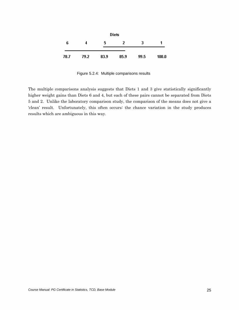
Figure 5.2.4 summarises the series of comparisons carried out in Table 5.2.3: any two means

that are connected by a line cannot be separated statistically, while those not so connected are

considered to be statistically significantly different. The size of the long-run mean difference

between any two diets is estimated by the confidence interval in Table 5.2.3.


25

Figure 5.2.4: Multiple comparisons results

The multiple comparisons analysis suggests that Diets 1 and 3 give statistically significantly

higher weight gains than Diets 6 and 4, but each of these pairs cannot be separated from Diets

5 and 2. Unlike the laboratory comparison study, the comparison of the means does not give a

‘clean’ result. Unfortunately, this often occurs: the chance variation in the study produces

results which are ambiguous in this way.


26

Tukey 95% Simultaneous Confidence Intervals

All Pairwise Comparisons among Levels of Diet

Individual confidence level9 = 99.54%

Diet = 1 subtracted from:

Diet Lower Center Upper ------+---------+---------+---------+---

2 -33.46 -14.10 5.26 (------*-------)

3 -19.86 -0.50 18.86 (-------*-------)

4 -40.16 -20.80 -1.44 (-------*------)

5 -35.46 -16.10 3.26 (-------*------)

6 -40.66 -21.30 -1.94 (------*-------)

------+---------+---------+---------+---

-25 0 25 50



3 -5.76 13.60 32.96 (------*-------)

4 -26.06 -6.70 12.66 (------*-------)

5 -21.36 -2.00 17.36 (-------*-------)

6 -26.56 -7.20 12.16 (-------*-------)

------+---------+---------+---------+---

-25 0 25 50



4 -39.66 -20.30 -0.94 (-------*-------)

5 -34.96 -15.60 3.76 (-------*-------)

6 -40.16 -20.80 -1.44 (-------*------)

------+---------+---------+---------+---

-25 0 25 50



5 -14.66 4.70 24.06 (-------*-------)

6 -19.86 -0.50 18.86 (-------*-------)

------+---------+---------+---------+---

-25 0 25 50



6 -24.56 -5.20 14.16 (-------*-------)

------+---------+---------+---------+---

-25 0 25 50

Table 5.2.3: Honestly significant differences between diets

9 This is the confidence level for individual comparisons which give confidence intervals of the same

width as the Tukey intervals which have a family confidence coefficient of 0.95 or 95%.


27

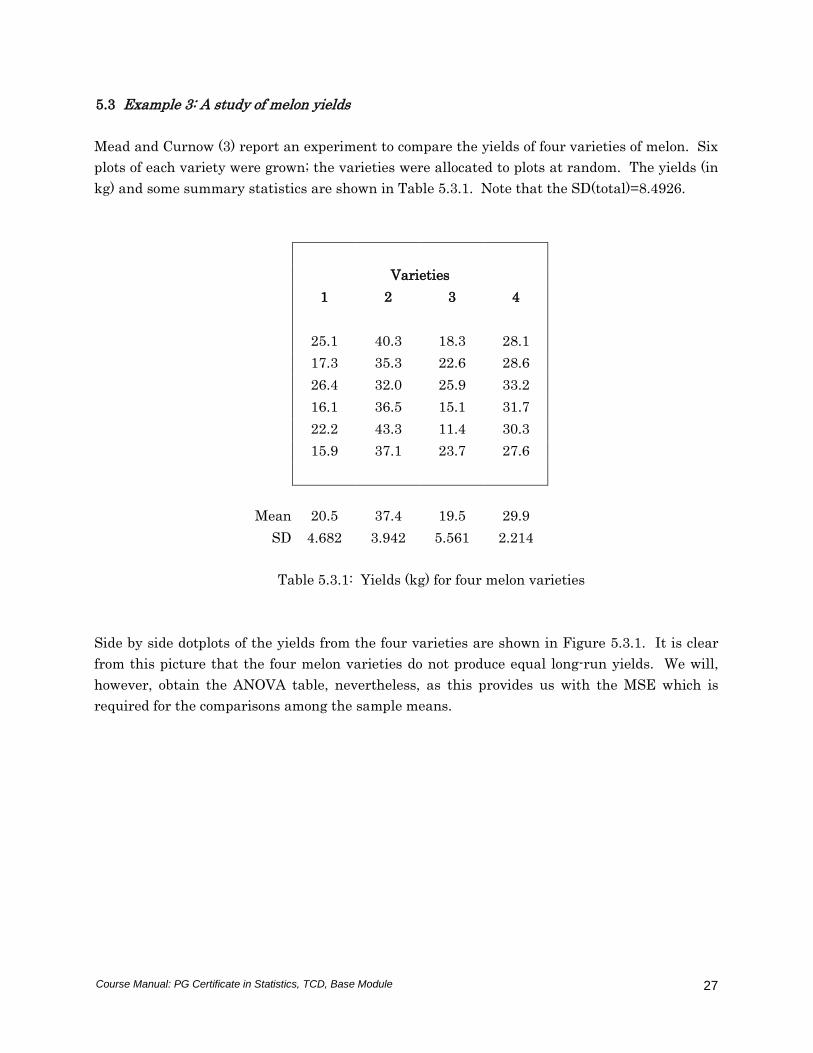
5.3 Example 3: A study of melon yields

Mead and Curnow (3) report an experiment to compare the yields of four varieties of melon. Six

plots of each variety were grown; the varieties were allocated to plots at random. The yields (in

kg) and some summary statistics are shown in Table 5.3.1. Note that the SD(total)=8.4926.

Varieties

1 2 3 4

25.1 40.3 18.3 28.1

17.3 35.3 22.6 28.6

26.4 32.0 25.9 33.2

16.1 36.5 15.1 31.7

22.2 43.3 11.4 30.3

15.9 37.1 23.7 27.6

Mean 20.5 37.4 19.5 29.9

SD 4.682 3.942 5.561 2.214

Table 5.3.1: Yields (kg) for four melon varieties

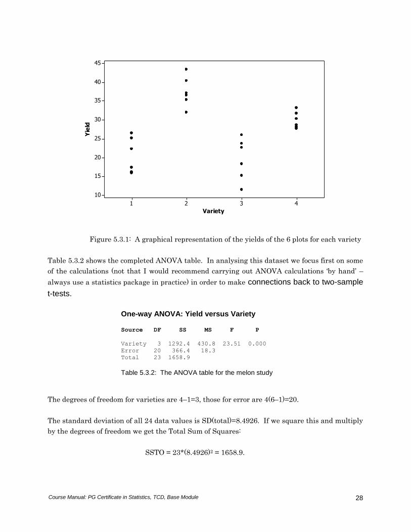
Side by side dotplots of the yields from the four varieties are shown in Figure 5.3.1. It is clear

from this picture that the four melon varieties do not produce equal long-run yields. We will,

however, obtain the ANOVA table, nevertheless, as this provides us with the MSE which is

required for the comparisons among the sample means.


28

4321

45

40

35

30

25

20

15

10

Variety

Yie

ld

Figure 5.3.1: A graphical representation of the yields of the 6 plots for each variety

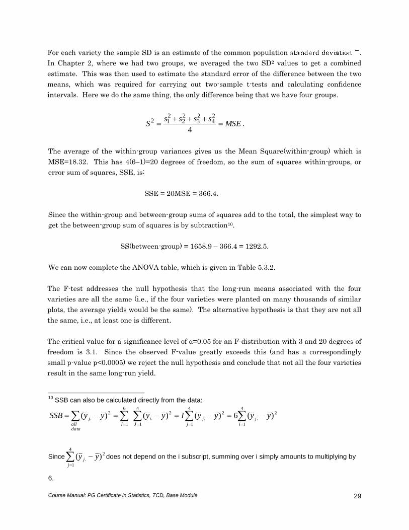
Table 5.3.2 shows the completed ANOVA table. In analysing this dataset we focus first on some

of the calculations (not that I would recommend carrying out ANOVA calculations ‘by hand’ –

always use a statistics package in practice) in order to make connections back to two-sample

t-tests.

One-way ANOVA: Yield versus Variety Source DF SS MS F P

Variety 3 1292.4 430.8 23.51 0.000

Error 20 366.4 18.3

Total 23 1658.9

Table 5.3.2: The ANOVA table for the melon study

The degrees of freedom for varieties are 4–1=3, those for error are 4(6–1)=20.

The standard deviation of all 24 data values is SD(total)=8.4926. If we square this and multiply

by the degrees of freedom we get the Total Sum of Squares:

SSTO = 23*(8.4926)2 = 1658.9.


29

For each variety the sample SD is an estimate of the common population

In Chapter 2, where we had two groups, we averaged the two SD2 values to get a combined

estimate. This was then used to estimate the standard error of the difference between the two

means, which was required for carrying out two-sample t-tests and calculating confidence

intervals. Here we do the same thing, the only difference being that we have four groups.

MSEssss

S

4

24

23

22

212

.

The average of the within-group variances gives us the Mean Square(within-group) which is

MSE=18.32. This has 4(6–1)=20 degrees of freedom, so the sum of squares within-groups, or

error sum of squares, SSE, is:

SSE = 20MSE = 366.4.

Since the within-group and between-group sums of squares add to the total, the simplest way to

get the between-group sum of squares is by subtraction10.

SS(between-group) = 1658.9 – 366.4 = 1292.5.

We can now complete the ANOVA table, which is given in Table 5.3.2.

The F-test addresses the null hypothesis that the long-run means associated with the four

varieties are all the same (i.e., if the four varieties were planted on many thousands of similar

plots, the average yields would be the same). The alternative hypothesis is that they are not all

the same, i.e., at least one is different.

The critical value for a significance level of α=0.05 for an F-distribution with 3 and 20 degrees of

freedom is 3.1. Since the observed F-value greatly exceeds this (and has a correspondingly

small p-value p<0.0005) we reject the null hypothesis and conclude that not all the four varieties

result in the same long-run yield.

10

SSB can also be calculated directly from the data:

2

.

4

1

2

.

4

1

2

.

4

1

6

1

2

. )(6)()()( yyyyIyyyySSB j

i

j

j

i

JI

j

dataall

Since2

.

4

1

)( yy j

j

does not depend on the i subscript, summing over i simply amounts to multiplying by

6.


30

Model Validation

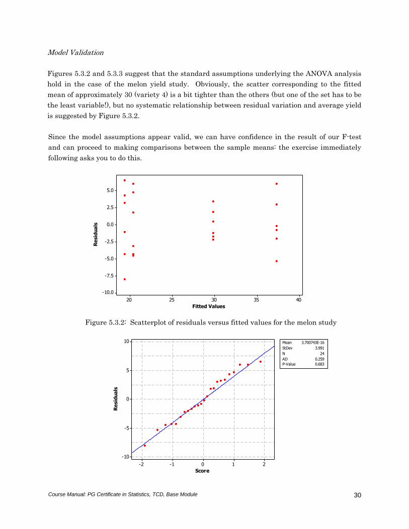
Figures 5.3.2 and 5.3.3 suggest that the standard assumptions underlying the ANOVA analysis

hold in the case of the melon yield study. Obviously, the scatter corresponding to the fitted

mean of approximately 30 (variety 4) is a bit tighter than the others (but one of the set has to be

the least variable!), but no systematic relationship between residual variation and average yield

is suggested by Figure 5.3.2.

Since the model assumptions appear valid, we can have confidence in the result of our F-test

and can proceed to making comparisons between the sample means: the exercise immediately

following asks you to do this.

4035302520

5.0

2.5

0.0

-2.5

-5.0

-7.5

-10.0

Fitted Values

Re

sid

ua

ls

Figure 5.3.2: Scatterplot of residuals versus fitted values for the melon study

10

5

0

-5

-10

210-1-2

Re

sid

ua

ls

Score

Mean 3.700743E-16

StDev 3.991

N 24

AD 0.259

P-Value 0.683


31

Figure 5.3.3: Normal plot of residuals for the melon study

Exercise 5.3.1

For the melons study:

Carry out a least significant difference analysis on the sample means and decide how

best to report your results.

Carry out a Bonferroni difference analysis on the sample means and decide how best to

report your results. Compare your results to those obtained from the least significant

difference analysis

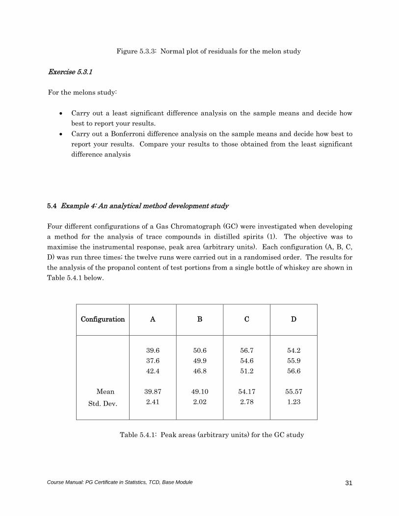
5.4 Example 4: An analytical method development study

Four different configurations of a Gas Chromatograph (GC) were investigated when developing

a method for the analysis of trace compounds in distilled spirits (1). The objective was to

maximise the instrumental response, peak area (arbitrary units). Each configuration (A, B, C,

D) was run three times; the twelve runs were carried out in a randomised order. The results for

the analysis of the propanol content of test portions from a single bottle of whiskey are shown in

Table 5.4.1 below.

Configuration

A

B

C

D

Mean

Std. Dev.

39.6

37.6

42.4

39.87

2.41

50.6

49.9

46.8

49.10

2.02

56.7

54.6

51.2

54.17

2.78

54.2

55.9

56.6

55.57

1.23

Table 5.4.1: Peak areas (arbitrary units) for the GC study


32

DCBA

55

50

45

40

35

Configuration

Pe

ak A

rea

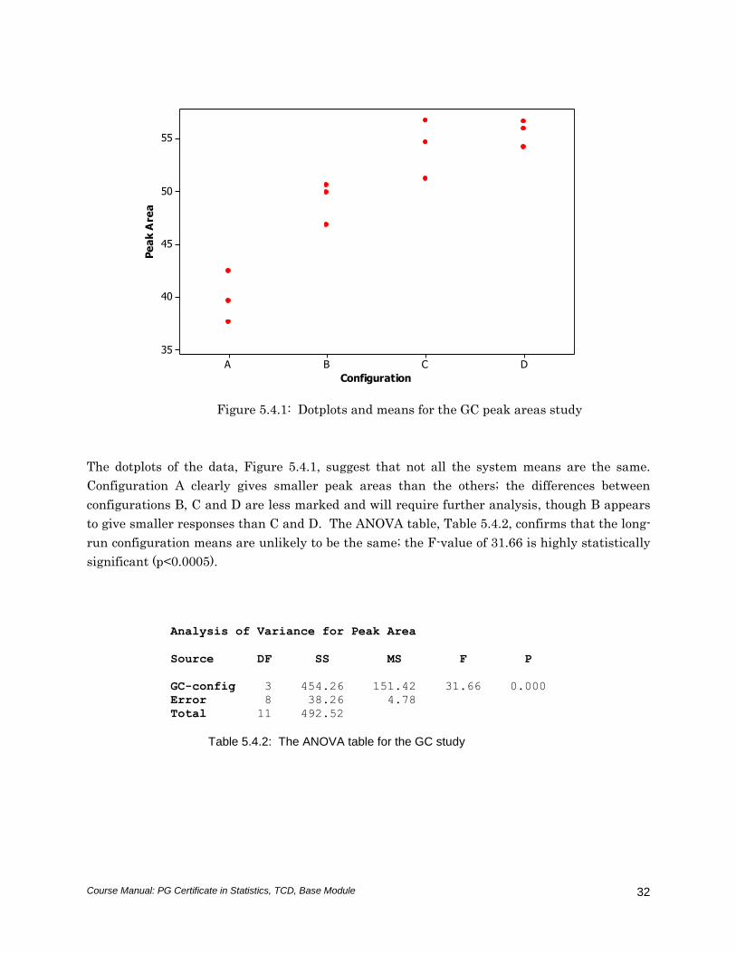
Figure 5.4.1: Dotplots and means for the GC peak areas study

The dotplots of the data, Figure 5.4.1, suggest that not all the system means are the same.

Configuration A clearly gives smaller peak areas than the others; the differences between

configurations B, C and D are less marked and will require further analysis, though B appears

to give smaller responses than C and D. The ANOVA table, Table 5.4.2, confirms that the long-

run configuration means are unlikely to be the same; the F-value of 31.66 is highly statistically

significant (p<0.0005).

Analysis of Variance for Peak Area

Source DF SS MS F P

GC-config 3 454.26 151.42 31.66 0.000

Error 8 38.26 4.78

Total 11 492.52

Table 5.4.2: The ANOVA table for the GC study


33

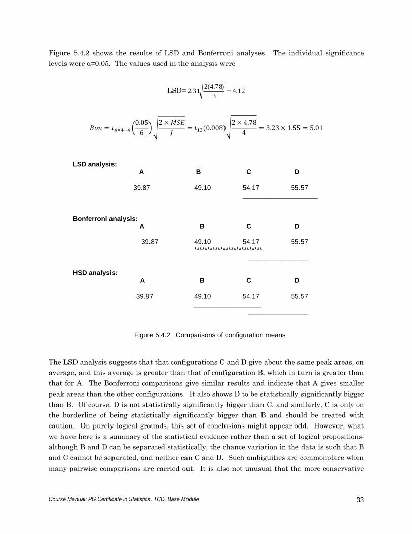
Figure 5.4.2 shows the results of LSD and Bonferroni analyses. The individual significance

levels were α=0.05. The values used in the analysis were

LSD= 12.43

)78.4(231.2

𝐵𝑜𝑛 = 𝑡4×4−4 (0.05

6) √

2 × 𝑀𝑆𝐸

𝐽= 𝑡12(0.008)√

2 × 4.78

4= 3.23 × 1.55 = 5.01

LSD analysis:

A B C D 39.87 49.10 54.17 55.57

____________________

Bonferroni analysis:

A B C D

39.87 49.10 54.17 55.57 ************************** ________________ HSD analysis:

A B C D

39.87 49.10 54.17 55.57 __________________ ________________

Figure 5.4.2: Comparisons of configuration means

The LSD analysis suggests that that configurations C and D give about the same peak areas, on

average, and this average is greater than that of configuration B, which in turn is greater than

that for A. The Bonferroni comparisons give similar results and indicate that A gives smaller

peak areas than the other configurations. It also shows D to be statistically significantly bigger

than B. Of course, D is not statistically significantly bigger than C, and similarly, C is only on

the borderline of being statistically significantly bigger than B and should be treated with

caution. On purely logical grounds, this set of conclusions might appear odd. However, what

we have here is a summary of the statistical evidence rather than a set of logical propositions:

although B and D can be separated statistically, the chance variation in the data is such that B

and C cannot be separated, and neither can C and D. Such ambiguities are commonplace when

many pairwise comparisons are carried out. It is also not unusual that the more conservative


34

Bonferroni (and HSD) method should fail to distinguish between pairs of means that are

reported as statistically significantly different when the LSD method is used.

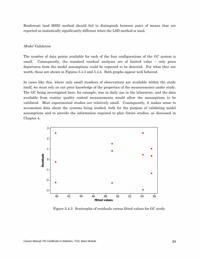
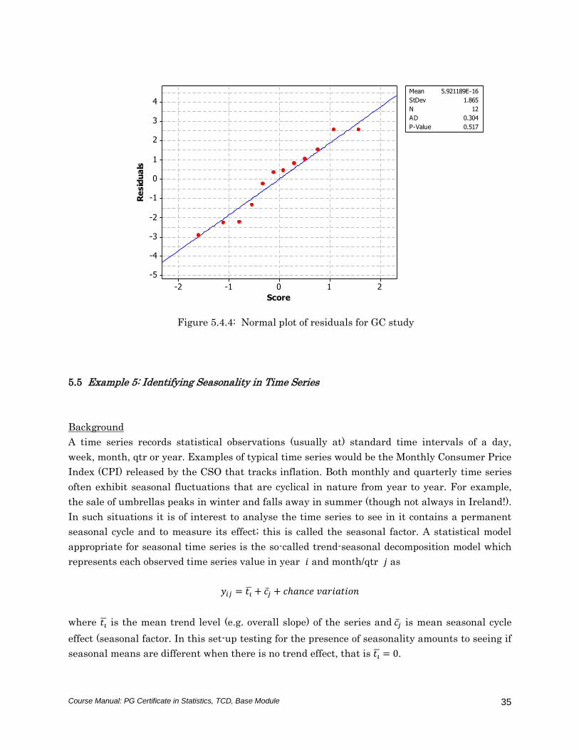
Model Validation

The number of data points available for each of the four configurations of the GC system is

small. Consequently, the standard residual analyses are of limited value – only gross

departures from the model assumptions could be expected to be detected. For what they are

worth, these are shown in Figures 5.4.3 and 5.4.4. Both graphs appear well behaved.

In cases like this, where only small numbers of observations are available within the study

itself, we must rely on our prior knowledge of the properties of the measurements under study.

The GC being investigated here, for example, was in daily use in the laboratory, and the data

available from routine quality control measurements would allow the assumptions to be

validated. Most experimental studies are relatively small. Consequently, it makes sense to

accumulate data about the systems being studied, both for the purpose of validating model

assumptions and to provide the information required to plan future studies, as discussed in

Chapter 4.

565452504846444240

3

2

1

0

-1

-2

-3

Fitted values

Re

sid

ua

ls

Figure 5.4.3: Scatterplot of residuals versus fitted values for GC study


35

4

3

2

1

0

-1

-2

-3

-4

-5

210-1-2

Re

sid

ua

ls

Score

Mean 5.921189E-16

StDev 1.865

N 12

AD 0.304

P-Value 0.517

Figure 5.4.4: Normal plot of residuals for GC study

5.5 Example 5: Identifying Seasonality in Time Series

Background

A time series records statistical observations (usually at) standard time intervals of a day,

week, month, qtr or year. Examples of typical time series would be the Monthly Consumer Price

Index (CPI) released by the CSO that tracks inflation. Both monthly and quarterly time series

often exhibit seasonal fluctuations that are cyclical in nature from year to year. For example,

the sale of umbrellas peaks in winter and falls away in summer (though not always in Ireland!).

In such situations it is of interest to analyse the time series to see in it contains a permanent

seasonal cycle and to measure its effect; this is called the seasonal factor. A statistical model

appropriate for seasonal time series is the so-called trend-seasonal decomposition model which

represents each observed time series value in year 𝑖 and month/qtr 𝑗 as

𝑦𝑖𝑗 = 𝑡�̅� + 𝑐�̅� + 𝑐ℎ𝑎𝑛𝑐𝑒 𝑣𝑎𝑟𝑖𝑎𝑡𝑖𝑜𝑛

where 𝑡�̅� is the mean trend level (e.g. overall slope) of the series and 𝑐�̅� is mean seasonal cycle

effect (seasonal factor. In this set-up testing for the presence of seasonality amounts to seeing if

seasonal means are different when there is no trend effect, that is 𝑡�̅� = 0.


36

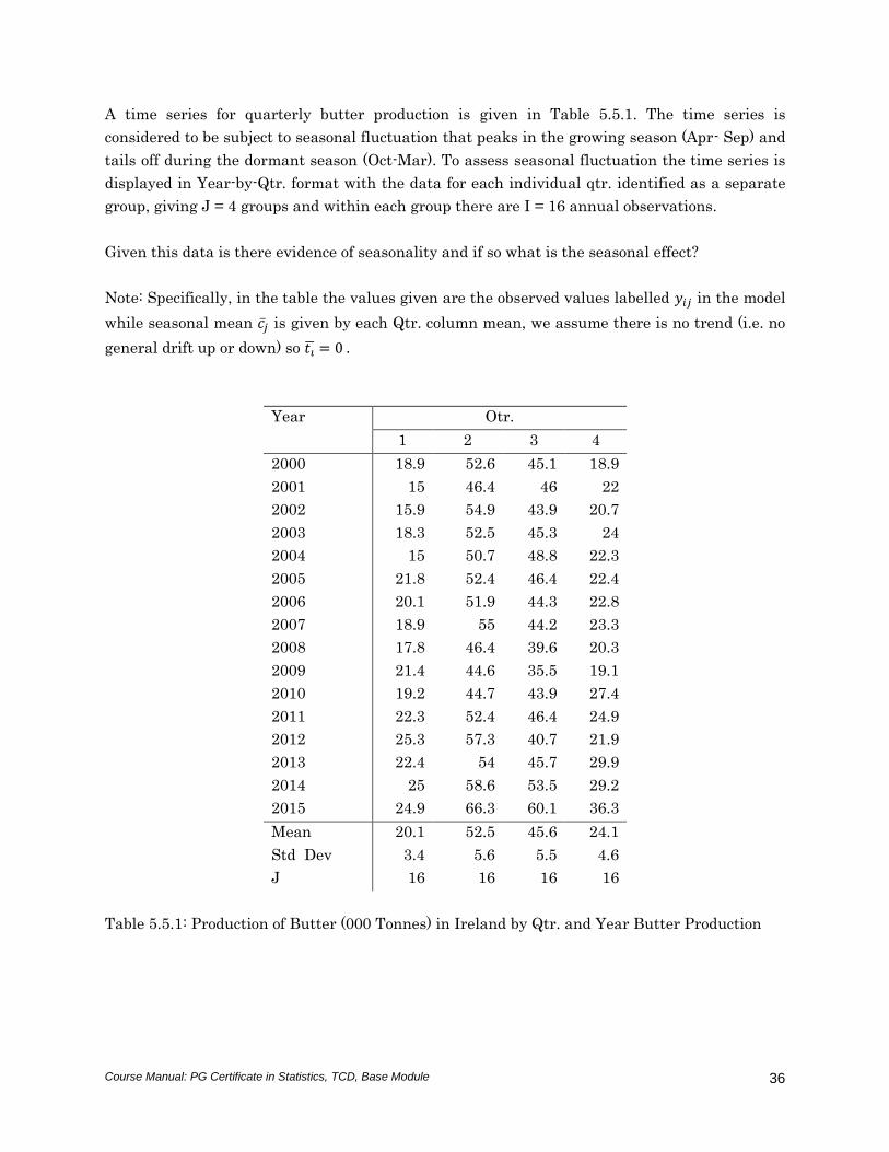
A time series for quarterly butter production is given in Table 5.5.1. The time series is

considered to be subject to seasonal fluctuation that peaks in the growing season (Apr- Sep) and

tails off during the dormant season (Oct-Mar). To assess seasonal fluctuation the time series is

displayed in Year-by-Qtr. format with the data for each individual qtr. identified as a separate

group, giving J = 4 groups and within each group there are I = 16 annual observations.

Given this data is there evidence of seasonality and if so what is the seasonal effect?

Note: Specifically, in the table the values given are the observed values labelled 𝑦𝑖𝑗 in the model

while seasonal mean 𝑐�̅� is given by each Qtr. column mean, we assume there is no trend (i.e. no

general drift up or down) so 𝑡�̅� = 0 .

Year Otr.

1 2 3 4

2000 18.9 52.6 45.1 18.9

2001 15 46.4 46 22

2002 15.9 54.9 43.9 20.7

2003 18.3 52.5 45.3 24

2004 15 50.7 48.8 22.3

2005 21.8 52.4 46.4 22.4

2006 20.1 51.9 44.3 22.8

2007 18.9 55 44.2 23.3

2008 17.8 46.4 39.6 20.3

2009 21.4 44.6 35.5 19.1

2010 19.2 44.7 43.9 27.4

2011 22.3 52.4 46.4 24.9

2012 25.3 57.3 40.7 21.9

2013 22.4 54 45.7 29.9

2014 25 58.6 53.5 29.2

2015 24.9 66.3 60.1 36.3

Mean 20.1 52.5 45.6 24.1

Std Dev 3.4 5.6 5.5 4.6

J 16 16 16 16

Table 5.5.1: Production of Butter (000 Tonnes) in Ireland by Qtr. and Year Butter Production


37

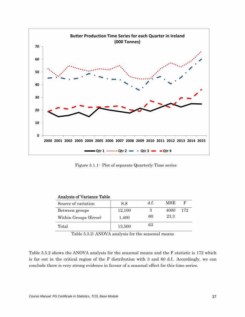
Figure 5.1.1: Plot of separate Quarterly Time series

Analysis of Variance Table

Source of variation S.S d.f. MSE F

Between groups 12,100 3 4000 172

Within Groups (Error) 1,400 60 23.3

Total 13,500 63

Table 5.5.2: ANOVA analysis for the seasonal means

Table 5.5.2 shows the ANOVA analysis for the seasonal means and the F statistic is 172 which

is far out in the critical region of the F distribution with 3 and 60 d.f.. Accordingly, we can

conclude there is very strong evidence in favour of a seasonal effect for this time series.

0

10

20

30

40

50

60

70

2000 2001 2002 2003 2004 2005 2006 2007 2008 2009 2010 2011 2012 2013 2014 2015

Qtr 1 Qtr 2 Qtr 3 Qtr 4

Butter Production Time Series for each Quarter in Ireland (000 Tonnes)


38

Bonferroni Analysis of seasonality, we have 𝑚 = (𝐽(𝐽−1)

2=

4(4−1)

2= 6 possible pairwise

comparisons, accordingly our adjusted 𝛼 value that is consistent with 𝛼 = 0.05 under the

ANOVA test is 𝛼 = 0.05/6, giving the Bonferroni difference

�̅�𝑗 − �̅�𝑘 = 𝑡𝐼𝐽−𝐽 (𝛼

𝑚) √

2 × 𝑀𝑆𝐸

𝐼

giving,

�̅�𝑖 − 𝑦 = 𝑡4×16−4 (0.05

6) √

2 × 𝑀𝑆𝐸

𝐼= 𝑡60(0.008)√

2 × 23.3

16

�̅�𝑗 − �̅�𝑘 = 2.77 × 1.71 = 4.74

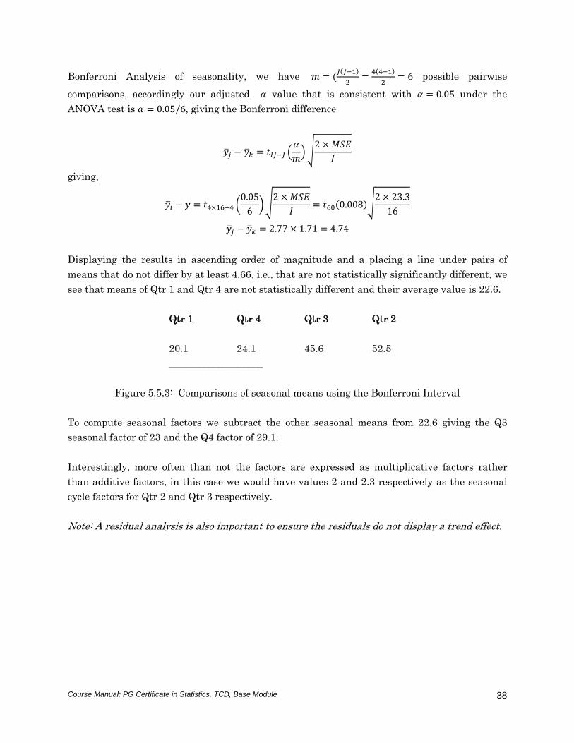
Displaying the results in ascending order of magnitude and a placing a line under pairs of

means that do not differ by at least 4.66, i.e., that are not statistically significantly different, we

see that means of Qtr 1 and Qtr 4 are not statistically different and their average value is 22.6.

Qtr 1 Qtr 4 Qtr 3 Qtr 2

20.1 24.1 45.6 52.5

___________________

Figure 5.5.3: Comparisons of seasonal means using the Bonferroni Interval

To compute seasonal factors we subtract the other seasonal means from 22.6 giving the Q3

seasonal factor of 23 and the Q4 factor of 29.1.

Interestingly, more often than not the factors are expressed as multiplicative factors rather

than additive factors, in this case we would have values 2 and 2.3 respectively as the seasonal

cycle factors for Qtr 2 and Qtr 3 respectively.

Note: A residual analysis is also important to ensure the residuals do not display a trend effect.


39

References

[1] Mullins, E., Statistics for the Quality Control Chemistry Laboratory, Royal Society of

Chemistry, Cambridge, 2003.

[2] Snedecor, G.W. and Cochran, W.G., Statistical Methods, Iowa State University Press,

6thed., 1967.

[3] Mead R., and Curnow, R.N., Statistical methods in agriculture and experimental biology,

London : Chapman and Hall, 1983.

Appendix: Tukey’s ‘Honestly Significant Difference’ (HSD) method

One multiple comparison method available in Minitab is Tukey’s ‘Honestly Significant

Difference’ (HSD). The derivation of the HSD interval is based on the range of a set of means,

i.e., the chance difference that we might expect to see, with a given probability, between the

largest and smallest values in the set, if the null hypothesis of equal long-run means for all

groups were true. If the largest and smallest means in a set differ by more than this amount

they will be considered statistically significantly different. Since all other differences between

pairs of means are, by definition, smaller than that between the largest and smallest means in

the set, any pair of means that differ by more than HSD are considered statistically

significantly different. Consequently, the significance level chosen applies to the whole family

of possible comparisons. The application of the HSD method is very similar to that of the LSD

method – it simply requires the replacement of the critical t-value (tc) by another multiplier (Tc),

which is given by:

))1(,,1(2

1 IJJqTc (5.10)

where q is the Studentised range distribution, α is the significance level for the family of

comparisons, J means are being compared and MSE has J(I-1) degrees of freedom.

For the laboratory study, Table ST-6 shows that requiring a family significance level of α=0.05

will lead to a critical Tc value of:

80.2)96.3(2

1)20,4,95.0(

2

1))1(,,1(

2

1 qIJJqTc . (5.11)


40

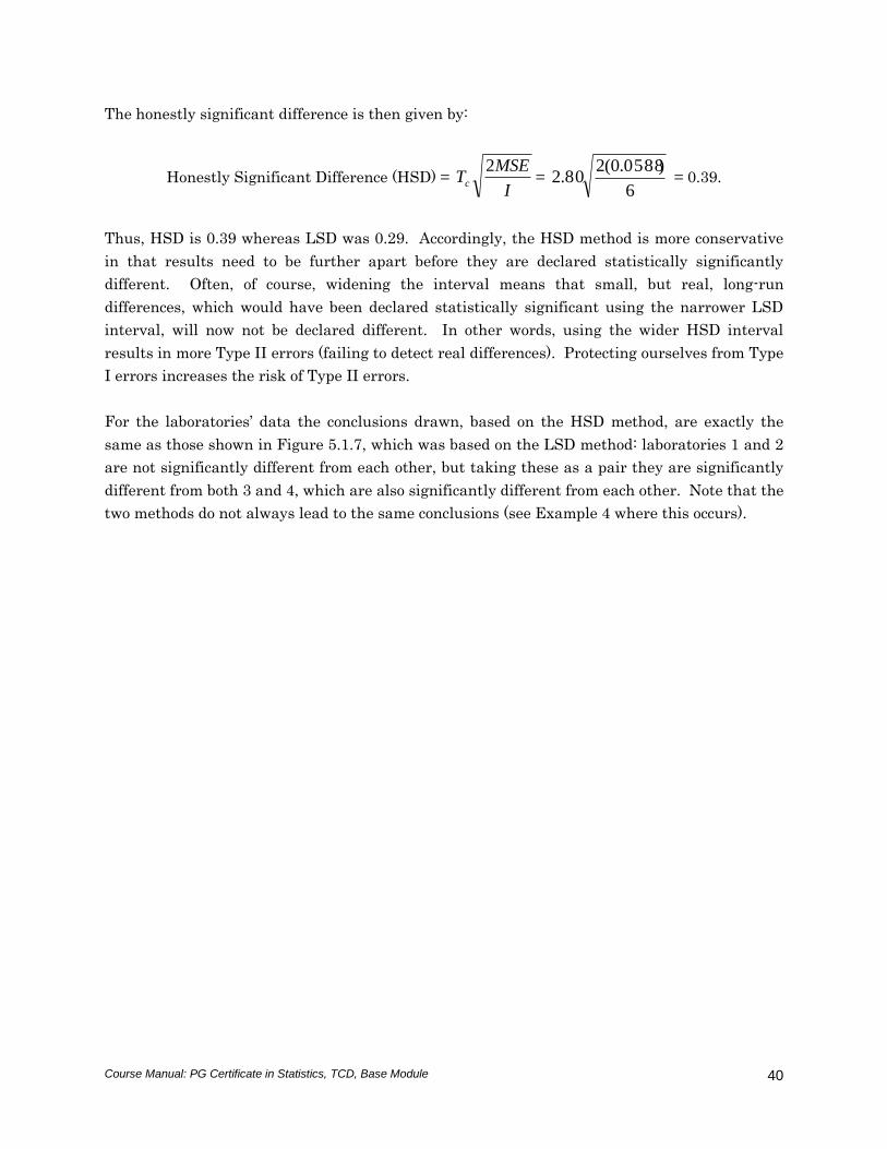
The honestly significant difference is then given by:

Honestly Significant Difference (HSD) = I

MSETc

2=

6

)0588.0(280.2 = 0.39.

Thus, HSD is 0.39 whereas LSD was 0.29. Accordingly, the HSD method is more conservative

in that results need to be further apart before they are declared statistically significantly

different. Often, of course, widening the interval means that small, but real, long-run

differences, which would have been declared statistically significant using the narrower LSD

interval, will now not be declared different. In other words, using the wider HSD interval

results in more Type II errors (failing to detect real differences). Protecting ourselves from Type

I errors increases the risk of Type II errors.

For the laboratories’ data the conclusions drawn, based on the HSD method, are exactly the

same as those shown in Figure 5.1.7, which was based on the LSD method: laboratories 1 and 2

are not significantly different from each other, but taking these as a pair they are significantly

different from both 3 and 4, which are also significantly different from each other. Note that the

two methods do not always lead to the same conclusions (see Example 4 where this occurs).


41

Outline Solutions

Exercise 5.1.1 (Iris Colour – critical flicker frequency study)

The ANOVA table for the critical flicker frequency study is shown below.

One-way ANOVA: CFF versus Iris Colour

Source DF SS MS F P

Iris Colour 2 22.69 11.35 5.79 0.014

Error 15 29.39 1.96

Total 17 52.08

Table 5.1.1.1: ANOVA table for the critical flicker frequency data

The critical value for an F test with a significance level of α=0.05 is 3.7 (the F distribution has 2,

15 degrees of freedom). The value given in the table (5.79) exceeds this, so we reject the null

hypothesis that all the corresponding population means are the same, and conclude that at least

one of them differs from the other two. The p-value of 0.014 is an alternative measure of

statistical significance – it tells us that our F value of 5.79 has an area of only 0.014 to its right,

which indicates that it would be an unusually large value if the null hypothesis were true.

LSD Analysis

The Least Significant Difference (LSD) is given by:

Least Significant Difference (LSD) = I

MSEtc

2=

6

)96.1(213.2 = 1.72.

The t-value used in the calculation has 15 degrees of freedom – the same as those of the MSE.

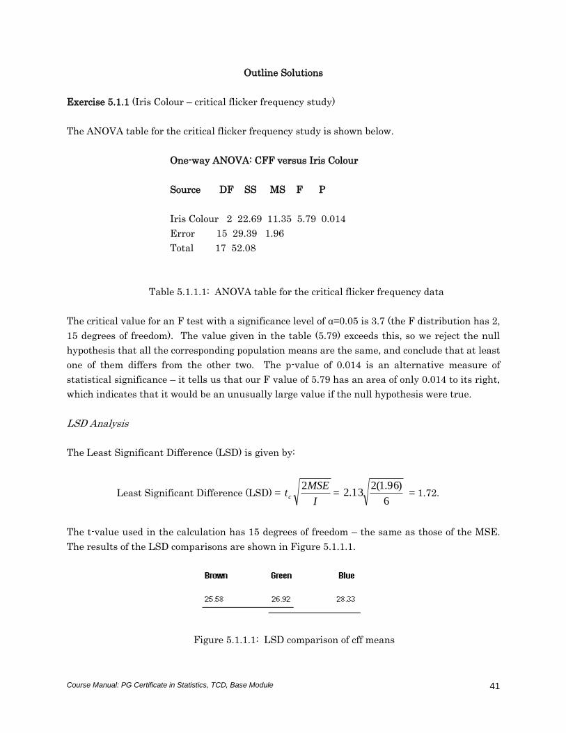
The results of the LSD comparisons are shown in Figure 5.1.1.1.

Figure 5.1.1.1: LSD comparison of cff means


42

The LSD is 1.72. Brown and Blue differ by more than this amount and so they are declared

statistically significantly different. Neither Brown and Green nor Green and Blue are different

by 1.72 so we cannot separate them statistically.

This was a small study – only six observations in each group – so we might not be surprised

that the outcome is not clear-cut. However, there is evidence that differences may exist and we

now have a basis for designing a larger study. The square root of the MSE is an estimate of the

standard deviation of person-to-person variation and it could be used to decide on an

appropriate sample size which would allow us to distinguish between Brown and Green or

Green and Blue (if differences truly exist), if the outcome of this study was considered

sufficiently interesting.

HSD Analysis

The Honestly Significant Difference (HSD) is given by:

Honestly Significant Difference (HSD) = I

MSETc

2.

Table ST-6 shows that requiring a family significance level of α=0.05 will lead to a critical Tc

value of:

6.2)67.3(2

1)15,3,95.0(

2

1))1(,,1(

2

1 qIJJqTc .

We then get:

HSD = 1.26

)96.1(26.2

2

I

MSETc .

Since Brown and Blue differ by more than this amount, the HSD analysis leads us to the same

conclusions as the LSD analysis and these are summarised in Figure 5.1.1.1


43

Exercise 5.3.1 (Melons study)

LSD Analysis

The ANOVA F-test in Example 3 established that differences exist between the mean yields of

the four melon varieties involved in the study. We now need to establish which means reflect

higher long-run yields. We will first use Fisher’s Least Significant Difference (LSD) and then

Bonferroni method to make the required comparisons between means. A confidence interval for

the difference between any pair of means is given by:

I

MSEtyy ckj

2)(

where I = 6 is the number of replicates in each group, MSE is the mean square error (the

estimate of the square of the common long-run standard deviation) and the critical t-value is tc

= 2.09 since there are 20 degrees of freedom for error; the quantity after the sign is the LSD =

16.5)47.2(09.26

)3.18(209.2 , the amount by which any pair of means must differ in order to be

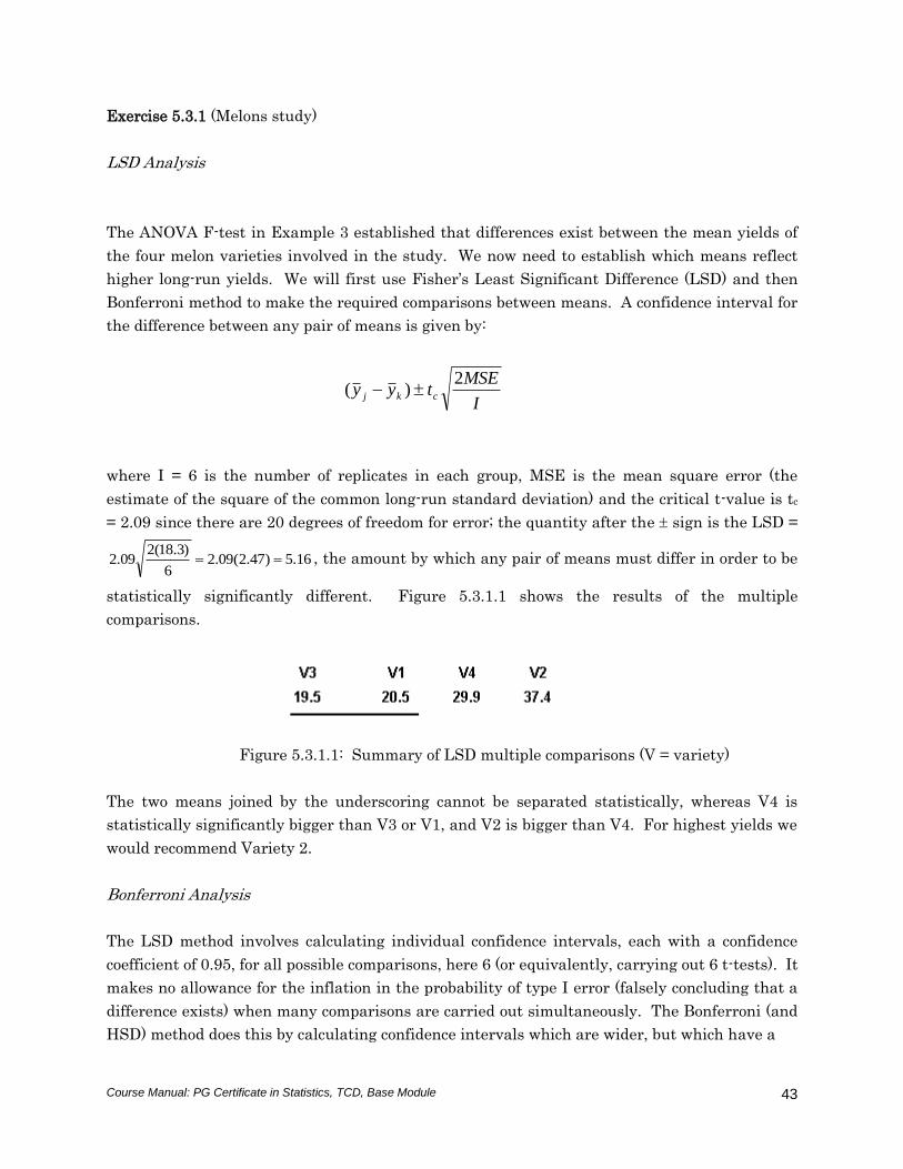
statistically significantly different. Figure 5.3.1.1 shows the results of the multiple

comparisons.

Figure 5.3.1.1: Summary of LSD multiple comparisons (V = variety)

The two means joined by the underscoring cannot be separated statistically, whereas V4 is

statistically significantly bigger than V3 or V1, and V2 is bigger than V4. For highest yields we

would recommend Variety 2.

Bonferroni Analysis

The LSD method involves calculating individual confidence intervals, each with a confidence

coefficient of 0.95, for all possible comparisons, here 6 (or equivalently, carrying out 6 t-tests). It

makes no allowance for the inflation in the probability of type I error (falsely concluding that a

difference exists) when many comparisons are carried out simultaneously. The Bonferroni (and

HSD) method does this by calculating confidence intervals which are wider, but which have a


44

coefficient of 0.95, i.e., all the intervals are expected to cover the corresponding true mean

differences, simultaneously, with this level of confidence. The method simply involves replacing

the critical t-value by:

𝑡𝑐𝑟𝑖𝑡 = 𝑡𝐼𝐽−𝐼 (𝛼

𝑚)

where 𝑚 = 𝐽(𝐽 − 1)/2. So, the Bonferroni allowable difference in group means is

�̅�𝑗 − �̅�𝑘 = 𝑡𝐼𝐽−𝐽 (𝛼

𝑚) √

2 × 𝑀𝑆𝐸

𝐼

We have 𝑚 =𝐽(𝐽−1)

2=

4(4−1)

2= 6, giving

�̅�𝑗 − �̅�𝑘 = 𝑡4×6−4 (0.05

6) √

2 × 𝑀𝑆𝐸

𝐼= 𝑡20(0.008)√

2 × 18.3

6

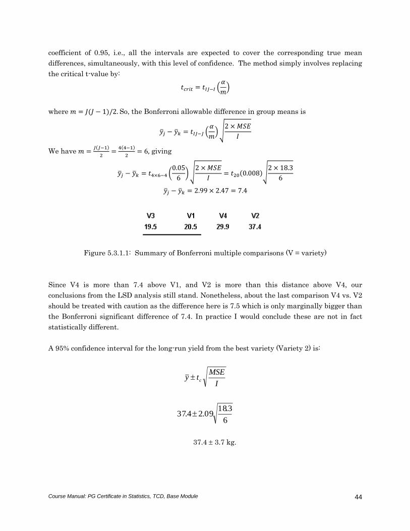
�̅�𝑗 − �̅�𝑘 = 2.99 × 2.47 = 7.4

Figure 5.3.1.1: Summary of Bonferroni multiple comparisons (V = variety)

Since V4 is more than 7.4 above V1, and V2 is more than this distance above V4, our

conclusions from the LSD analysis still stand. Nonetheless, about the last comparison V4 vs. V2

should be treated with caution as the difference here is 7.5 which is only marginally bigger than

the Bonferroni significant difference of 7.4. In practice I would conclude these are not in fact

statistically different.

A 95% confidence interval for the long-run yield from the best variety (Variety 2) is:

I

MSEty c

6

3.1809.24.37

37.4 3.7 kg.

Documents

Analysis of Variance: an introduction - Trinity College, … 5: Analysis of Variance: an introduction to one-way ANOVA 5.0 Introduction In Chapter 2 we used two-sample t-tests based