Analysis of Wireless Power Transfer by Coupled Mode Theory (CMT

2

Analysis of Wireless Power Transfer by Coupled Mode Theory (CMT) and

Practical Considerations to Increase Power Transfer Efficiency

Alexey Bodrov and Seung-Ki Sul IEEE Fellow,

Republic of Korea

1. Introduction

In this chapter the analytical model of a wireless power transfer scheme is developed

through the means of Coupled Mode Theory (CMT). The derivation is made under the

assumption of low internal coil losses and some particular type of resonator (coil inductance

and capacitance) equivalent circuit.

With the equivalent circuit modeling the wireless power transfer system the direct high

frequency power source connection to the source coil and the usage of external capacitance

are considered. It is shown that the maximum efficiency to resonant frequency ratio could

be obtained by serial to short end antenna connection of external capacitance.

At MHz frequencies especially near and at the resonant frequencies, the calculation of coil

parameters which are the coefficients of the model obtained by means of CMT is not a trivial

task. Equivalent resistance, capacitance and inductance of antenna become frequency

dependent, and those should be specially considered. Because the equivalent resistance is a

critical parameter for the efficiency maximization, the skin and proximity effects are

included and the verification of the calculation process is presented. Also due to frequency

dependence of equivalent inductance and capacitance, the procedure to obtain the optimal

resonant frequency of antennas in terms of the efficiency of the power transfer is discussed.

2. Theoretical analysis of wireless power transfer scheme

In figure 1 a typical diagram of wireless power transfer system is shown. In this system, the

inductive reactance and the capacitive reactance of each coil has equal magnitude at the

resonant frequency, causing energy to oscillate between the magnetic field of the inductor

and the electric field of the capacitor (considering both internal and external capacitances of

the coil). The energy transmission occurs due to intersection of magnetic field of the source

coil and the load coil. There is no intersection of electric fields, because all electrical energy

concentrates in the capacitor (it could be easily shown through Gauss' law of flux).

There are many ways to analyze the wireless power system but here the scattering matrix approach and CMT will be discussed.

www.intechopen.com

Wireless Power Transfer – Principles and Engineering Explorations

20

Fig. 1. Typical diagram of wireless power transfer system.

2.1 Efficiency calculation of the wireless power transfer system with scattering matrix’s parameters

The wireless power transfer scheme could be analyzed with the two-port network theory, which is formulated in figure 2. As discussed in [1], such networks could be characterized by various equivalent circuit parameters, such as transfer matrix, impedance matrix in (1) and scattering matrix in (2).

Fig. 2. Two-port network scheme.

1 2 1 11 12 1

21 221 2 2 2

transfer matrix impedance matrix

V A B V V Z Z I

C D Z ZI I V I

⎡ ⎤ ⎡ ⎤ ⎡ ⎤ ⎡ ⎤⎡ ⎤ ⎡ ⎤= =⎢ ⎥ ⎢ ⎥ ⎢ ⎥ ⎢ ⎥⎢ ⎥ ⎢ ⎥ −⎣ ⎦ ⎣ ⎦⎣ ⎦ ⎣ ⎦ ⎣ ⎦ ⎣ ⎦'*(*) '*(*) (1)

where V1 and V2 are the input and output voltages of the network and similarly I1 and I2 are

the input and output currents with the direction specified as in a figure 2. Scattering matrix

relates the ingoing (s+1,2) and the outgoing waves (s-1,2) of the network.

1 11 12 1

21 222 2

scatering matrix

s S S s

S Ss s− +− +

⎡ ⎤ ⎡ ⎤⎡ ⎤=⎢ ⎥ ⎢ ⎥⎢ ⎥⎣ ⎦⎣ ⎦ ⎣ ⎦'*(*) (2)

In electric circuit analysis, transfer and impedance matrices are widely used, but the

measurement of coefficients becomes difficult at higher frequencies. Instead, a scattering

matrix is preferred due to the existence of network analyzers, which can measure scattering

matrix parameters over a wide range of frequencies.

Employing this two-port network concept, the efficiency of power transfer between the

generator and the load can be calculated as followings [1].

www.intechopen.com

Analysis of Wireless Power Transfer by Coupled Mode Theory (CMT) and Practical Considerations to Increase Power Transfer Efficiency

21

Fig. 3. Two port network connected to the power supply and a load.

From the scattering matrix analysis, the expression for the voltages and currents in terms of wave variables can be presented as (3).

( ) ( )( ) ( )

1 0 1 1 2 0 2 2

1 1 1 2 2 20 0

1 1

V Z s s V Z s s

I s s I s sZ Z

+ − + −

+ − + −

= + = += − = − (3)

where Z0 is the reference impedance value (normally chosen to be 50Ω). Considering figure 3 and (3) it is possible to define scattering matrix equations as (4).

1 1

2 2

in

L

V Z I

V Z I

== ⇔ 1 1

2 2

in

L

s Г s

s Г s− +− +== (4)

where Zin is the input network impedance and Гin, ГL are the reflection coefficients given by (5).

0

0

0

0

inin

in

LL

L

Z ZГZ Z

Z ZГZ Z

−= +−= +

(5)

From (3)-(5) it is possible to define reflection coefficients in terms of scattering matrix parameters.

12 2111

221L

inL

S S ГГ SS Г

= + − (6)

Following the procedure in Ref.[1], if the roles of the generator and the load are reversed, two more reflection coefficients can be derived as (7)

0 0

0 0

out Gout G

out G

Z Z Z ZГ ГZ Z Z Z

− −= =+ + (7)

where Zout is the output impedance. And the reflection coefficients in (7) also depend on the scattering matrix parameters as (8).

12 2122

111G

outG

S S ГГ SS Г

= + − (8)

www.intechopen.com


22

The efficiency of the wireless power transfer can be deduced through the Pin (input power, coming into the two port network from the generator) and Pout (output power, going out from the two port network to the load). For the system in figure 3 from Ref.[1] the input and

output power can be derived as

( )( )

2

2

2 221

2

11

1

2

1

2

G inin

in G

G LL

G out L

V RP

Z Z

V R ZP

Z Z Z Z

= += + +

(9)

where Rin=Re{Zin} and RL=Re{ZL}. In here “Re” stands for the real part of the complex number. From (9), a necessary condition for maximum power delivery from the generator to the connected system is given by (10).

Zin= *GZ (10)

Similarly the maximum output power could be delivered to the load when (11) holds.

ZL= *outZ (11)

Then in terms of S-parameters, the efficiency of wireless power transfer from Ref.[1] could be deduced as (12).

( ) ( )

( )( )2 2 2

21

1 2

11 22 12 21

1 1

1 1

G L

G L G L

Г S Г

S Г S Г S S Г Гη − −= − − − (12)

Here, if the load and generator impedances are matched to the reference impedance (i.e. ZG=ZL=Z0), then from (7) and (8) reflection coefficients would be presented as (13).

11 220 and , L G in outГ Г Г S Г S= = = = (13)

Substituting (13) to (12) the efficiency formula can be simplified as (14).

2

1 21Sη = (14)

2.2 Analysis based on the Coupled Mode Theory (CMT)

This section describes the CMT analysis. At first basic definitions for a simple LC circuit are introduced, and by sequentially adding losses, a full wireless power transfer system model including coupling effect is obtained.

2.2.1 Basic definitions

This book utilizes the resonance phenomena for the efficient wireless power transfer. Generally, resonance can take many forms: mechanical resonance, acoustic resonance,

electromagnetic resonance, nuclear magnetic resonance, electron spin resonance, etc. The wireless power transfer relies on the electromagnetic resonance and it is discussed by means

www.intechopen.com


23

of CMT. The presented coupled mode formalism is general and developed in more detail in Ref. [2].

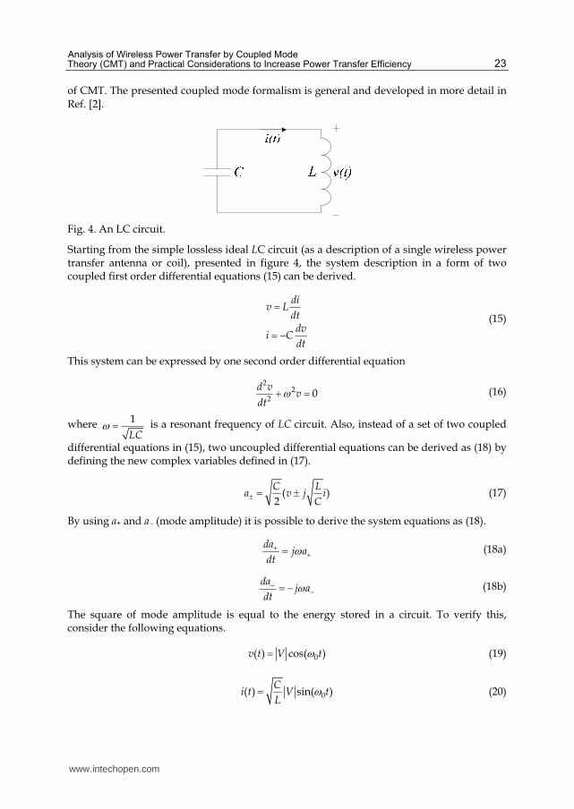
Fig. 4. An LC circuit.

Starting from the simple lossless ideal LC circuit (as a description of a single wireless power transfer antenna or coil), presented in figure 4, the system description in a form of two coupled first order differential equations (15) can be derived.

div L

dtdv

i Cdt

== −

(15)

This system can be expressed by one second order differential equation

2

22

0d v

vdt

ω+ = (16)

where 1

LCω = is a resonant frequency of LC circuit. Also, instead of a set of two coupled

differential equations in (15), two uncoupled differential equations can be derived as (18) by defining the new complex variables defined in (17).

( )2

C La v j i

C± = ± (17)

By using a+ and a - (mode amplitude) it is possible to derive the system equations as (18).

daj a

dtω+ += (18a)

daj a

dtω− −= − (18b)

The square of mode amplitude is equal to the energy stored in a circuit. To verify this, consider the following equations.

0( ) cos( )v t V tω= (19)

0( ) sin( )C

i t V tL

ω= (20)

www.intechopen.com


24

where |V| is a peak amplitude of voltage in figure 4. Substituting (19) and (20) in (17), the mode amplitude, a, can be derived as

00 0( cos( ) sin( ))

2 2j tC C

a V t j V t V e ωω ω+ = + = (21)

Hence,

2 2

2

Ca V W+ = = (22)

where W is the energy stored in the circuit. And similar procedure can be applied to a-. The main advantage of such transformations is the possibility to represent the system of

coupled differential equations in a form of two uncoupled equations like (19). Moreover it is

possible to use only one equation (18a) to describe the resonant mode, since the second one,

(18b) is the complex conjugate form of (18a). Therefore in further analysis subscript + will be

dropped and only equation (18a) will be used.

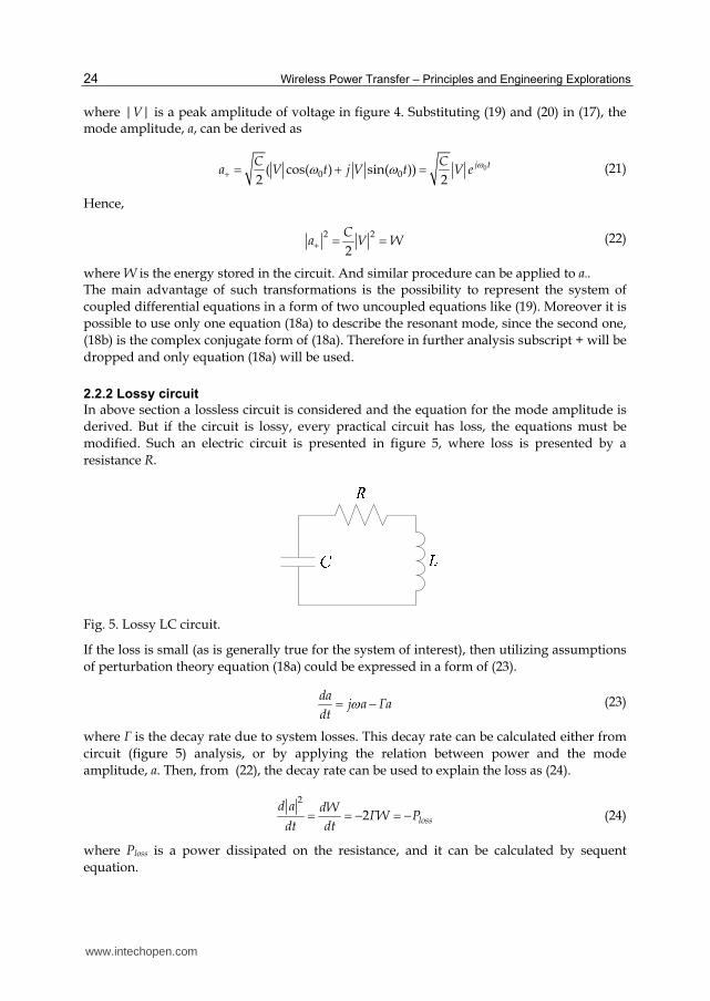
2.2.2 Lossy circuit

In above section a lossless circuit is considered and the equation for the mode amplitude is

derived. But if the circuit is lossy, every practical circuit has loss, the equations must be

modified. Such an electric circuit is presented in figure 5, where loss is presented by a

resistance R.

Fig. 5. Lossy LC circuit.

If the loss is small (as is generally true for the system of interest), then utilizing assumptions

of perturbation theory equation (18a) could be expressed in a form of (23).

daj a Гa

dtω= − (23)

where Г is the decay rate due to system losses. This decay rate can be calculated either from

circuit (figure 5) analysis, or by applying the relation between power and the mode

amplitude, a. Then, from (22), the decay rate can be used to explain the loss as (24).

2

2 loss

d a dW ГW Pdt dt

= = − = − (24)

where Ploss is a power dissipated on the resistance, and it can be calculated by sequent

equation.

www.intechopen.com


25

21

2loss

WRP I R

L= = (25)

Thus unloaded (with no external load) quality factor Q of such a system can be expressed as (26).

2loss

W LQ

P Г R

ω ωω= = = (26)

Hence decay rate Г could be derived from (26) as (27).

2

RГL

= (27)

Other perturbations (coupling with other resonator, connection to the transmission line, etc) as discussed in Ref.[2] could be added in a similar manner to the intrinsic circuit loss.

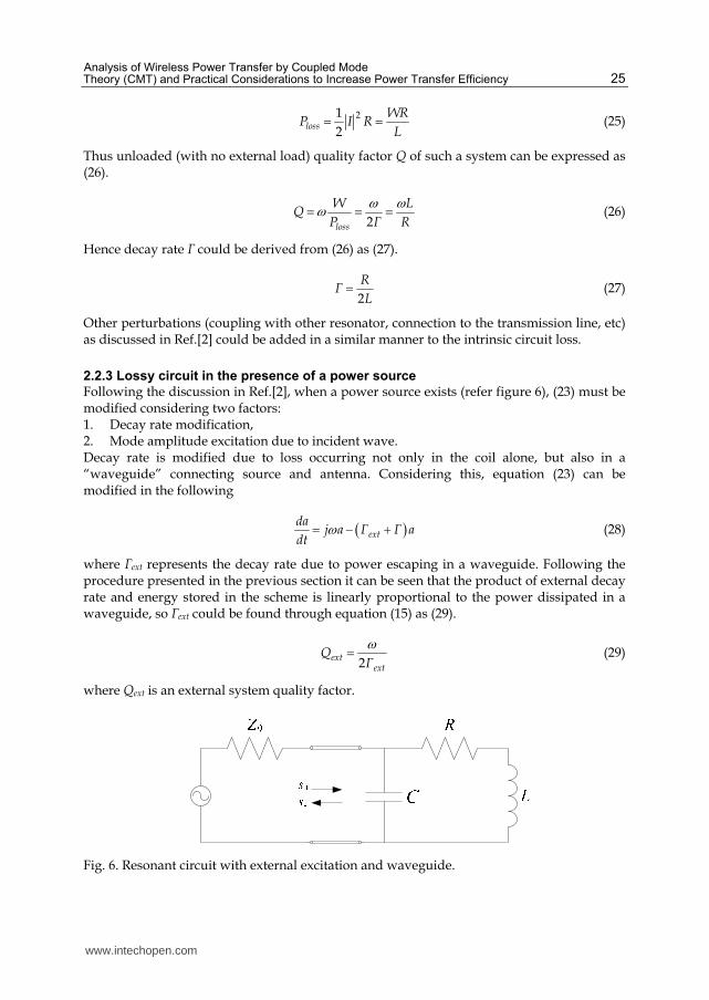
2.2.3 Lossy circuit in the presence of a power source

Following the discussion in Ref.[2], when a power source exists (refer figure 6), (23) must be modified considering two factors: 1. Decay rate modification, 2. Mode amplitude excitation due to incident wave. Decay rate is modified due to loss occurring not only in the coil alone, but also in a “waveguide” connecting source and antenna. Considering this, equation (23) can be modified in the following

( )ext

daj a Г Г a

dtω= − + (28)

where Гext represents the decay rate due to power escaping in a waveguide. Following the procedure presented in the previous section it can be seen that the product of external decay rate and energy stored in the scheme is linearly proportional to the power dissipated in a waveguide, so Гext could be found through equation (15) as (29).

2

extext

QГω= (29)

where Qext is an external system quality factor.

Fig. 6. Resonant circuit with external excitation and waveguide.

www.intechopen.com


26

Further, considering the excitation by incident wave, (28) must be modified as (30).

( )ext

daj a Г Г a Ks

dtω += − + + (30)

where K expresses the degree of coupling between source and coil, and s+ represents the

incident wave incoming to the antenna. It is important to mention that 2s+ has the

meaning of input power, rather than energy as in case of 2a .Using reversibility property of

Maxwell’s equations, it is possible to show that

2 extK Г= (31)

Therefore, by applying (31) to (30), that the resonator mode is described by three parameters: self-resonant frequency ω, internal (Г) and external (Гext) decay rates as (32).

( ) 2ext ext

daj a Г Г a Г s

dtω += − + + (32)

2.2.4 Coupling of two lossless resonant circuits

C1 L1 C2L2

M

i1(t) i2(t)

v1(t) v2(t)

Source coil Load coil

Fig. 7. Coupled resonators.

Presented formalism can be readily expanded to describe the coupling of two resonant circuits. Suppose that a1 and a2 are the mode amplitudes of uncoupled lossless resonators with resonant frequencies ω1 and ω2, respectively. Then, if the resonators are coupled through some perturbation, (in the case of wireless power transfer it is the mutual inductance M), for the first resonator (18a) can be expressed as (33a).

11 12 2

daj a k a

dtω= + (33a)

Consequently for the second resonator (18a) is transformed to (33b)

22 21 1

daj a k a

dtω= + (33b)

where k12 and k21 are the coupling coefficients between the modes. Energy conservation law described in (34) provides a necessary condition for k12 and k21.

www.intechopen.com


27

1 2

1

1 2 1

* *2 2 * *1 2

1 2 1 2 2

* * * * * *12 2 1 12 2 21 1 2 21

( )

0

da dad da daa a a a a a

dt dt dt dt dt

a k a a k a a k a a k a

+ = + + + == + + + =

(34)

From (34), since “amplitudes of a1 and a2 can be set arbitrarily” [1], the coupling coefficients

must satisfy the sequent condition.

*12 21 0k k+ = (35)

Similar to necessary conditions, exact values of k12 and k21 could be obtained through energy

conservation considerations. From the equation (33b) the power transferred from the first

resonator to the second resonator through the mutual inductance M (see figure 7) can be

evaluated as (36).

2

2 * * *21 21 1 2 21 1 2

d aP k a a k a a

dt= = + (36)

But from the electric circuit analysis for the circuit in figure 7 power flowing through M can

be expressed as (37).

1 221 2

( )d i iP i M

dt

−= (37)

Then, by introducing complex current envelope quantities 1( )I t , 2( )I t , an expression for

current i1(t) can be written as in the following.

1 1*1 1 1

1( ) ( ( ) ( ) )

2

j t j ti t I t e I t eω ω−= + (38)

A similar procedure can be applied to the expression for current i2(t), then by substituting

both of these currents into (37), the expression for transferred power can be rewritten as

( )2 2 1 1 2 2* * *21 2 2 1 1 2 2

1( ( ) ( ) ) ( ) ( ) ( ) ( )

4j t j t j t j t j t j td

P I t e I t e I t e I t e I t e I t edt

ω ω ω ω ω ω− − −⎛ ⎞= + + − −⎜ ⎟⎝ ⎠ (39)

In (39), 11

j tdI e

dtω⎛ ⎞⎜ ⎟⎝ ⎠ terms are much smaller than the jωI1, so they can be ignored. By such a

approximation, (39) can be modified (40)

( )1 2 1 2( ) ( )* *21 1 1 2 1 1 2

1

4j t j tP j MI I e j MI I eω ω ω ωω ω− − −= − (40)

Then, comparing (40) with (36) and defining2

nj tnn n

La I e ω= , where n=1,2, the coupling

coefficient can be derived as (41).

121

1 22

j Mk

L L

ω= (41)

www.intechopen.com


28

Equation (41) yields that k21 is a purely complex number, so due to (35), k21 can be derived as (42).

21 121 22

j Mk k jk

L L

ω= = = (42)

where ω must be interpreted as arithmetic mean 1 2

2

ω ω+ or geometric mean 1 2ω ω of the

corresponding coil’s self resonance frequencies.

2.2.5 Full wireless power transfer system model

In figure 8 the scheme of the wireless power transfer system is depicted. Here ZG stands for the internal impedance of the power source and d represents the distance between the source and load coils.

Fig. 8. Wireless power transfer scheme.

Incorporating the results presented in the above sections, the full model of such a system by CMT can be represented as follows,

( )

1 1

11 1 1 1 2

22 2 2 2 1

( )( ) ( ) ( ) 2 ( )

( )( ) ( ) ( )

ext ext

da tj a t Г Г a t jka t Г s t

dtda t

j a t Г a t jka tdt

ωω

+= − + + += − +

(43)

However, (43) still cannot express a full wireless power transfer system, because it does not contain term representing load. If the load is considered by defining |s+n(t)|2 as power ingoing to the object n (n=1,2) and |s-n(t)|2 as power outgoing from the resonant object n, the full system can be described as (44).

( )( )

1 1

2

1

2

11 1 1 1 2 1

22 2 2 2 1

1 1 1

2 2

( )( ) ( ) ( ) 2 ( )

( )( ) ( ) ( )

( ) 2 ( ) ( )

( ) 2 ( )

ext ext

ext

ext

ext


dtda t

j a t Г Г a t jka tdt

s t Г a t s t

s t Г a t

ωω

+

− +−

= − + + += − + += −=

(44)

www.intechopen.com


29

2.3 Finite-amount power transfer Supposing “no source” and “no load” conditions, the system description (44) modifies to (45).

11 1 1 2

22 2 2 1

( )( ) ( ) ( )

( )( ) ( ) ( )

da tj a t Г a t jka t

dtda t

j a t Г a t jka tdt

ωω

= − += − +

(45)

where index 1 stands for the source coil and 2 - for the load coil. (45) can be rewritten in another form as (46).

( ) ( )a t Aa t=f f$ (46)

where ( )a tf

is a vector which involves the mode amplitudes of the source coil and the load

coil. And matrix A is defined as (47).

1 1

2 2

j Г jkA

jk j Гω

ω−⎛ ⎞= ⎜ ⎟−⎝ ⎠ (47)

Eigen-values of such system could be obtained through solving the characteristic equation, det(A-sI)=0. They can be presented in (48).

221 2 1 2 1 2 1 2

1

221 2 1 2 1 2 1 2

2

2 2 2 2

2 2 2 2

Г Г Г Гx j j j k

Г Г Г Гx j j j k

ω ω ω ω

ω ω ω ω

+ + − −⎛ ⎞= − + − +⎜ ⎟⎝ ⎠+ + − −⎛ ⎞= − − − +⎜ ⎟⎝ ⎠

(48)

The eigen-values are complex and distinct so the solution for resonance modes will be in form of (49).

( ) 1 211 1 2 2

2

( )

( )x t x ta t

a t c V e c V ea t

⎛ ⎞= = +⎜ ⎟⎝ ⎠f (49)

where c1 and c2 are constants determined by the initial conditions and V1,V2 are eigen-vectors. For the simplicity of further discussion, the constant 0Ω is defined as (50).

2

21 2 1 20

2 2

Г Гj k

ω ω− −⎛ ⎞Ω = − +⎜ ⎟⎝ ⎠ (50)

By such a transformation, eigen-vectors can be calculated as follows,

2 1 2 10

1

2 1 2 10

2

1

2 2

1

1

2 2

1

Г Гj

V k

Г Гj

V k

ω ω

ω ω

⎛ ⎞− −⎛ ⎞− + −Ω⎜ ⎟⎜ ⎟= ⎝ ⎠⎜ ⎟⎜ ⎟⎝ ⎠⎛ ⎞− −⎛ ⎞− + + Ω⎜ ⎟⎜ ⎟= ⎝ ⎠⎜ ⎟⎜ ⎟⎝ ⎠

(51)

www.intechopen.com


30

Assuming that the source coil at time t=0 has energy |a1(0)|2 and at the same time energy contained in the load coil is |a2(0)|2. Then, by inserting (48),(50),(51) to (49) the resonant modes can be presented as (52).

1 2 1 2

1 2

2 1 2 1 2 21 1 0 0 0 2 0

0 0 0

2 1 2 1 22 1 0 2 0 0 0

0 0 0

( ) (0) cos( ) sin( ) sin( ) (0) sin( )2 2

( ) (0) sin( ) (0) cos( ) sin( ) sin( )2 2

Г Гj t t

j

jkГ Гa t a t t j t a t e e

jk Г Гa t a t a t t j t e

ω ω

ω ω

ω ω

ω ω

+ +−

+

⎛ ⎞⎛ ⎞− −= Ω + Ω − Ω + Ω ⋅⎜ ⎟⎜ ⎟⎜ ⎟Ω Ω Ω⎝ ⎠⎝ ⎠⎛ ⎞⎛ ⎞− −= Ω + Ω − Ω + Ω ⋅⎜ ⎟⎜ ⎟⎜ ⎟Ω Ω Ω⎝ ⎠⎝ ⎠

1 2

2

Г Гt te

+− (52)

Note that, for a special case when ω1=ω2=ω0 and Г1=Г2=Г0 (for the equal source and load antennas) and |a2(0)|2=0 (52) can be simplified to a set of equations as (53).

0 0

0 0

1 1

2 1

( ) (0)cos( )

( ) (0)sin( )

j t Г t

j t Г t

a t a kt e e

a t ja kt e e

ωω

−−

== (53)

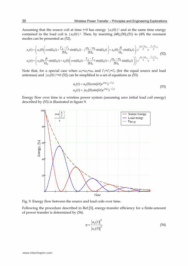
Energy flow over time in a wireless power system (assuming zero initial load coil energy) described by (53) is illustrated in figure 9.

20

40

60

80

100

So urce Energy

Lo ad E nerg y

Decay

So urce Energy

Lo ad E nerg y

Decay

2

2

atank

Γ⎛⎜⎝

⎞⎟⎠k

Fig. 9. Energy flow between the source and load coils over time.

Following the procedure described in Ref.[3], energy-transfer efficiency for a finite-amount of power transfer is determined by (54).

( )( )

2

2

2

1 0

a t

aη = (54)

www.intechopen.com


31

Then by defining 0

kU

Г= and T=Г0t the time t° which maximizes efficiency is calculated

through maximization of ( )( )2

1

sin( )0

T a tUT e

a−⋅ = . Utilizing Lagrange method, optimal time in

the sense of maximum energy transfer time can be calculated by the following equation

atan

atan( ) or

k

U ГT t

U kο ο

⎛ ⎞⎜ ⎟⎝ ⎠= = (55)

Then, substitution of (55) to (54) results in optimal transfer efficiency as (56).

( ) ( )2atan2

21

U

UU

t eU

οη−

= + (56)

It is important to note that (56) represents the optimal transfer efficiency which is only dependent on U (“coupling to loss ratio” [3]) and tends to be unity when U»1. Although a finite-amount power transfer scheme is pure theoretical, one could consider it to be a conceptual power transfer system, where the power source is connected to the source coil at time t=0 for a very short time and then at time t=t° the load would drain energy from the load coil. This procedure would repeat.

2.4 Wireless power transfer in the presence of source and load

This section considers the case when a power source is continuously connected to the source

coil through 1extГ and the load is correspondingly connected to the load coil through

2extГ .

Equations for wireless power transfer defining such a case was already described in 2.2.5.

Here, they are repeated for the convenience of future system efficiency calculations.

( )( )

1 1

2

1

2

11 1 1 1 2 1

22 2 2 2 1

1 1 1

2 2

( )( ) ( ) ( ) 2 ( )

( )( ) ( ) ( )

( ) 2 ( ) ( )

( ) 2 ( )

ext ext

ext

ext

ext


dtda t

j a t Г Г a t jka tdt

s t Г a t s t

s t Г a t

ωω

+

− +−

= − + + += − + += −=

(44)

Similar to the discussion in Ref.[3], it assumes that the excitation frequency is fixed and equal to ω. And, the field amplitudes has the form of (57).

( )1 1j ts t S e ω+ += (57)

where S+1 is some constant determined by the amplitude of incident wave. Then it is possible to express the system (44) in matrix form as follows,

( ) ( )

( ) ( ) 11 1

12 2

2( )

0

( ) 1 1

extГj Г jka t a t s t

jk j Г

y t a t

ωω +

⎛ ⎞−⎛ ⎞ ⎜ ⎟= +⎜ ⎟ ⎜ ⎟−⎝ ⎠ ⎝ ⎠=

f f$

f f (58)

www.intechopen.com


32

The transfer function of the system (58) can be derived as (59).

( ) ( )( ) 1 2 2

2 21 2 1 2 1 2 1 2 2 1 1 2

2ˆ

extГ s j Г jkg s

s s j j Г Г j Г j Г Г Г k

ωω ω ω ω ω ω

− + −= − + + + − − − + + (59)

And it has a pair of poles 1,2s defined in (60).

( )( )2 21 2 1 21,2 1 2 2 1

14

2 2 2

Г Гs j j Г Г k

ω ω ω ω+ += − + ± − + − − (60)

From (60), it is apparent that for the typical parameters of interest, poles of transfer function (59) always have negative real parts, so the system (58) is Boundary Input Boundary Output (BIBO) stable. BIBO stability together with (57) imply that the response of a linear system

( ( )a tf

) will be at the same frequency ω as the input and could be represented in the form of

(61).

( )1,2 1,2j ta t A e ω= (61)

A similar discussion for s-1,2(t) leads to the conclusion that the expression for the outgoing waves has the same form as (61) and can be represented as (62).

( )1,2 1,2j ts t S e ω− −= (62)

By substituting (61) and (62) into (44) and taking into account the time derivative of (62)

such as ( ) ( )1,2 1,2 1,2j ta t j A e j a tωω ω−= =$ , it is possible to calculate transmission coefficient S21

(from the scattering matrix). By defining 1,2 1,2δ ω ω= − , 1,21,2

1,2

DГδ= , 1,2

1,21,2

extГU

Г= and

1 2

kU

Г Г= , S21 can be expressed as (63).

1 2

1 2

1 2221 2 2

1 1 1 2 2 1 1 2 2

2 2

( )( ) (1 )(1 )

ext ext

ext ext

jk Г Г jU U UsS

s Г Г j Г Г j k U jD U jD Uδ δ−+

= = =+ + + + + + + + + + (63)

Similarly, the reflection coefficient S11, can be determined (“field amplitude reflected to the generator” [3]).

1 2

1 2

2 21 1 2 2 1 1 2 21

11 2 21 1 1 2 2 1 1 2 2

( )( ) (1 )(1 )

( )( ) (1 )(1 )

ext ext

ext ext

Г Г j Г Г j k U jD U jD UsS

s Г Г j Г Г j k U jD U jD U

δ δδ δ−

+− + + + + − + + + += = =+ + + + + + + + + + (64)

Other parameters of the scattering matrix can be obtained simply by interchanging notations 1 and 2 due to the reciprocity property. The purpose of this present discussion is to find the optimal parameters which will maximize the efficiency as determined by the maximum ratio of power between the power “obtained” by the load and the power “sent” by the source. The conditions can be found solving the following problems:

www.intechopen.com


33

1. Power transmission efficiency maximization (i.e. 2

21 maxS → )

2. Power reflection minimization at generator side/load side (i.e. 2

11 minS → )

2.4.1 Maximization of power transmission efficiency

As discussed in the preceding section, to obtain maximum transmission efficiency, 2

21S

must be maximized. From (63), it can be determined that this expression is symmetric by

interchanging 1↔2. Therefore, optimal values for D1 and D2 must be the same as like U1 and

U2. By defining D0=D1=D2 and U0=U1=U2, (63) is transformed into (65).

021 2 2

0 0

2

(1 )

jUUS

U jD U= + + + (65)

From here, by utilizing Lagrange method it is possible to obtain optimal values for D0 (for fixed values of U and U0). Power transmission efficiency could be maximized by setting D0 as (66).

2 2

* 0 00

0

(1 ) 1

0, 1

U U if U UD

if U U

⎧⎪± − + > += ⎨ ≤ +⎪⎩ (66)

Further, with this optimal *0D , by the similar procedure it is possible to show that the

optimal value for U0 is expressed as (67).

* 20 1U U= + (67)

From figure 10 cited from Ref.[3], it can be seen that the matching of condition in (67) is very important to maximize the power transfer efficiency. In this figure the system efficiency

Fig. 10. Efficiency of wireless power transfer scheme as a function of U0 and detuning D0[3].

(a) (b)

www.intechopen.com


34

versus frequency for different values of 0*0

U

U is presented. From this graph maximum

efficiency is obtained when U0=*0U , and the physical meaning of “over-coupled” defined as

the system where *0 0>U U and “under-coupled” as *

0 0<U U becomes clear.

From (66), the optimal value of D0 can only be 0. So substituting this result together with

(67) into (65), the optimal power transmission efficiency is given by (68).

( ) 2

* * *0 0

2,

1 1

UD U

Uη η ⎛ ⎞= = ⎜ ⎟⎜ ⎟+ +⎝ ⎠

(68)

From (68), it is important to mention that efficiency is again just a function of U ,where

1 2

kU

Г Г= , and it approaches unity as U increases to infinity.

Note that, in a real system, the strict satisfaction of all the optimal conditions is very difficult

or even impossible. For example, from (67) it can be said that the optimal U0 should be set

by U. However U0 is determined by the source and load and is therefore not controllable.

Moreover, U is dependent on the distance of power transfer. Referring to figure 10(b), when

the system is over-coupled to achieve maximum efficiency (at two peaks on the figure) the

frequency of the power source must not be the same with the resonant frequencies of objects

( *0 0D ≠ ). That is why it is significant to find these new optimal power supply frequencies.

The optimal frequency which will maximize the power transmission efficiency in this case is

derived as (69).

1 2

1 2

1 2

1 2 21 2 2 11 2

1 2 1 2 1 2 1 2

1 2 2 1

1 2 1 2 1 2

2( )( ) , if 1 1

, if 1 1

ext extext ext

ext ext

Г ГГ ГГ Г kk Г Г Г Г

Г Г Г Г Г Г Г Г

Г ГГ Г k

Г Г Г Г Г Г

ω ωω ω ω±

⎧ ⎛ ⎞⎛ ⎞+⎪ ± − + + > + +⎜ ⎟⎜ ⎟+ +⎪ ⎝ ⎠⎝ ⎠⎪= ⎨⎪ ⎛ ⎞⎛ ⎞+ ≤ + +⎜ ⎟⎜ ⎟⎪ + ⎝ ⎠⎝ ⎠⎪⎩

(69)

In (69), the first equation for the power supply frequency ω corresponds to the over-coupled

system, the second – to under-coupled system. To indicate this regime of operation given by

(69) the term “semi-optimal conditions” can be used. Note, that if we define δsp=ω+-ω- (splitting

of frequencies), then for the same resonant objects (i.e.1 2 01 2 0 and ext ext extГ Г Г Г Г Г= = = = )

splitting of frequencies will be described as (70).

( ) 0

2202sp extk Г Гδ = − + (70)

And this becomes a criterion for the coupling coefficient k value calculation.

2.4.2 Minimization of power reflection

Minimization of the reflection of the powers can be achieved by minimization of 2

11S [3].

From (64), conditions of 2

11S minimization are formulated as (71).

* * 21,2 1,2 11,22 1 1 2 2, : 0 (1 )(1 ) 0D U S U jD U jD U= ⇒ + ± + + =∓ (71)

www.intechopen.com


35

Similar to the discussion regarding equation (71) in 2.4.1, it is symmetric by interchanging

1↔2. And it can be said that the optimal values for D1,2 are the same and equal to some new1 *0D (as with U1,2). Substituting these considerations into (71) results in (72).

2 2 20 0(1 ) 0jD U U+ − + = (72)

Equation (72) (which equally represents the impedance matching problem in terms of CMT)

results in the optimal conditions for *0D and *

0U , as (73).

*0

* 20

0

1

D

U U

== + (73)

Accordingly, both power transmission efficiency maximization and power reflection minimization at both the generator side and load side lead to the same set of conditions described by (73). Therefore, the following does not divide the term “efficiency” into parts, instead it includes both meanings.

2.5 Efficient wireless power transfer: Scattering matrix analysis vs. CMT results

In above sections, the conditions for efficiency maximization, based on two different approaches (scattering matrix analysis and CMT), are presented. From section 2.1, the scattering matrix analysis, the three conditions used to maximize efficiency are given by (74):

*

**in L

"No reflection" conditionZ =Z

Symmetric condition

in s

out L

s L

Z Z

Z Z

Z Z

⎫⎫= ⎪ ⎪⎬ ⎪⎬= ⎪⎭ ⎪= ⎪⎭ (74)

From section 2.2, for the CMT, the two conditions which maximize efficiency are given by (75).

* * *1 2 0

* * * 21 2 0

0

1

D D D

U U U U

= = == = = + (75)

The variables that are used to describe the optimal conditions in (74) and (75) are different.

So the question naturally arises “do these conditions contradict to each other?” To answer

this question, an equivalent circuit of a wireless power system connected to the source and

load can be considered as shown in figure 11.

In figure 11 Rac1 and Rac2 represent coil losses and M stands for the mutual inductance

between the coils. In addition, Rs is an internal source impedance and RL , the load

impedance. Cext1 and Cext2 represent the external capacitors connected to the antennas

(internal capacitance of the coil is neglected). Supposing that Rs=RL and the coils are the

same (due to the equivalence of coils, subscripts 1,2 are omitted in following discussion).

1 It would be shown that optimal conditions for sections 2.4.1 and 2.4.2 are absolutely same. So it is not required to introduce a new variable for current discussion.

www.intechopen.com


36

Fig. 11. Equivalent circuit of wireless power transfer in lumped parameters.

This assumption automatically leads to the satisfaction of the symmetric condition given by

(74) and provides that 1 2D D= and 1 2U U= .

With these considerations, condition (74) for the circuit in figure 11 can be developed as (76).

( )

( )2 2 2 2 2

1( )

1( )

1

or

2 22 0

L

in L

L

L

j M R R j L Mj C

Z R j L M Rj C R R j L

j C

R LR R M L j LR

j C C

ω ω ωω ω ω ω

ω ω ω

⎛ ⎞+ + − +⎜ ⎟⎝ ⎠= + − + + =+ + +

− + − + + + = (76)

And if the resonance type of operation is considered (i.e. 1

LCω = ), (76) can be simplified

to

2

2 2L

MR R

LC= + (77)

Meanwhile, from (75), the assumption of resonant operation leads to * * *1 2 0 0D D D= = = . In

order to represent the second condition of CMT in terms of figure 11 (78) can be derived.

and LR MU U

R R

ω= = (78)

Substituting (78) into the second equation of (75) results in the following,

2

2 2L

MR R

LC= + (79)

Equation (79) is exactly same to (77) which was obtained through scattering matrix analysis of the circuit. As shown above, both theories give the same result so any of them can be used as a basis for maximum power transfer research. In here, CMT would be used to explain the phenomenon of the wireless power transfer, because S-parameters (scattering matrix’s elements) are not easily predicted, and because the system design based on scattering matrix is problematic. So, the usage of S-parameters is restricted to the experimental verification of results, due to the simple experimental calculation of the S-matrix by a network analyzer. Also, some papers

www.intechopen.com


37

have proposed the wireless power system can be described by the conventional circuit analysis. However, this method is too complicated to utilize in this field (for example, in the case of indirect feeding). Moreover, such an analysis is not universal and will vary from a circuit to another circuit. For example, if external capacitance is added to the coil, the whole model must be recalculated. In contrast, CMT provides an accurate and convenient way of modeling of the system and, as it was presented in section 2.4, expresses the system as a set of linear differential equations given by (80).

( ) ( )

( ) ( ) 11 1

12 2

2( )

0

( ) 1 1

extГj Г jka t a t s t

jk j Г

y t a t

ωω +

⎛ ⎞−⎛ ⎞ ⎜ ⎟= +⎜ ⎟ ⎜ ⎟−⎝ ⎠ ⎝ ⎠=

f f$

f f (80)

Here, it is important to note that CMT is based on several assumptions. First, the internal loss of coils is comparatively small (to satisfy the perturbation theory requirements). Second, the frequency range of operation is narrow enough to assume inductance and internal capacitance of the coils be constant. Third, “overall field profile can be described as a superposition of the modes due to each object” [4].

3. Analysis of a real system by CMT & practical considerations to increase efficiency

As presented in a section 2, 1 2

kU

Г Г= , (69) is the figure of merit to maximize the efficiency

of the power transfer. Also, in the same section, the quality factor of each coil is defined as

2Q

Гω= , (26). By rearranging two equations, the following relationship can be obtained.

1 21 2

U

kU K Q Q

Г Г= = (81)

where KU is a coupling factor between two coils (

1 2U

MK

L L= ) and Q1 and Q2 are the quality

factors of the source and load coils, respectively. From equation (81), to achieve a high figure of merit U (i.e. to get maximum efficiency), one should use resonant coils with a high quality factor (or with a low intrinsic loss rate Г). Another way to increase efficiency is to make a tight coupling between two resonators. However, in practical applications there is always a geometrical limit of object size, and it applies restriction to KU and Qn magnification. In the following sections, ways of calculating Qn and KU will be presented together with ways to increase the figure of merit U.

3.1 Capacitive-loaded helical coils

In Ref.[3], [5] and [6], wireless power transfer by resonant coils without external capacitance was widely discussed and practical implementation was shown. For example, in Ref.[5] wireless power transfer between coils over 2 meters distance with a maximum 40% efficiency was reported. But the frequencies of such a power transfer exceed 10MHz, which may be costly in designing such a high frequency power source. Here, the goal is to reduce

www.intechopen.com


38

the operational frequency of power transfer. One solution to reduce the resonant frequency of object is to add a large external capacitor (“large external capacitor” means that its value exceeds the coil’s self-capacitance). Such systems have been discussed in Ref.[3] and Ref.[7]. In figure 12, a capacitive-loaded helical coil is presented. In order to calculate the quality factor of such a coil the inductance, self capacitance, and resistance must be evaluated.

Cext

Fig. 12. Diagram of capacitive-loaded helical coil.

3.1.1 Inductance, self-capacitance and resistance of a helical coil

Following the procedure presented in Ref.[8], the calculation of the quality factor starts from the inductance evaluation of the helical coil. The concept of the lumped inductance is strictly applicable only at low frequencies, i.e. when the length of wire consisting coil is much smaller than the wavelength of the frequency. This means that waves enter into the input terminal of the antenna and come out from the output terminal with virtually no phase difference. Obviously, this is not true at high frequencies. When speaking about the inductance of a coil at high frequencies, it is useful to segregate the discussion into two parts: external inductance due to the magnetic energy stored in a surrounding medium and internal inductance due to the magnetic field stored inside the wire itself.

Fig. 13. Diagram of current-sheet inductor.

www.intechopen.com


39

Inductance calculations are normally started from analysis of a so-called current-sheet inductor, as shown in figure 13. Such a solenoid is assumed to have an infinitely thin conducting wound wire (one layer) with no spacing between the turns (nevertheless the turns are electrically isolated). The main characteristic of such a coil is that at low frequencies they have a uniform magnetic field distribution along their length. If all these assumptions are satisfied, the expression for the inductance can be expressed as (82):

2 2

4s

Diam nL

h

μπ= (82)

where Diam is the coil diameter, n – number of turns, h – height of the coil and ┤ is magnetic permeability, which in the absence of a core reduces to ┤0. The current-sheet inductor is a theoretical model, but by using this model the formula for

the real inductors could be obtained after the introduction a few modifications. The

modifications can be divided into two parts: frequency independent and frequency

dependent. The first consists of a field non-uniformity correction coefficient (kL), a self

induction correction coefficient for a round wire (ks) and a mutual inductance correction

coefficient for a wound wire (km). The frequency dependent parameters which must be taken

in consideration are Diam (effective loop diameter), internal inductance (Li) and self-

capacitance (C).

3.1.2 Frequency independent modifications

In figure 14 a real coil is depicted, where wires forming the coil have some finite size (round

wire with radius a and height h) and there is non-zero spacing between the coil turns (p is

the pitch of the coil)

2a

Dia

m a+

Dia

m w

Diama Diam

a -D

iamw

p

h

Fig. 14. Inductor with finite size, made from round wire [8].

When coil length is comparable to its diameter, the assumption of uniform field distribution

is not valid. In 1909 H.Nagaoka introduced coefficient kL [9] to consider this non-uniformity

(83).

www.intechopen.com


40

2 4

2

2 4 6

4 1ln 1 0.383901 0.017108

2

21 0.258952

0.093842 0.002029 0.000801

L

Diam h h

h Diam Diam

h hkDiam Diam

h h h

Diam Diam Diam

π

⎛ ⎞⎛ ⎞⎛ ⎞⎛ ⎞ ⎛ ⎞ ⎛ ⎞⎜ ⎟− + +⎜ ⎟⎜ ⎟ ⎜ ⎟ ⎜ ⎟⎜ ⎟⎜ ⎟⎜ ⎟⎝ ⎠ ⎝ ⎠ ⎝ ⎠⎝ ⎠⎝ ⎠⎜ ⎟⎛ ⎞⎜ ⎟= + ⎜ ⎟⎜ ⎟⎝ ⎠⎜ ⎟⎜ ⎟⎛ ⎞ ⎛ ⎞ ⎛ ⎞+ + −⎜ ⎟⎜ ⎟ ⎜ ⎟ ⎜ ⎟⎝ ⎠ ⎝ ⎠ ⎝ ⎠⎝ ⎠

(83)

With this correction, (82) can be modified to the following equation.

2 2

4s L

Diam nL k

h

μπ= (84)

However, for the real coils, a coefficient, ks, to consider the round shape of the wire must be added, and, moreover, another coefficient, km, to consider the mutual inductance between the adjacent turns must be included. To take these factors into account, E.B.Rosa [10] modified (84) to a new expression (85).

( )2

s s m

nDiamL L k k

μ= − + (85)

where

( ) 3 5

7 9

3ln

2

3 ln( ) 0.33084236 1 1ln 2

2 6 120 5040.0011923 0.0005068

-

s

m

pk

a

nk

n n n n

n n

π

⎛ ⎞= − ⎜ ⎟⎝ ⎠= − − − − +

+ (86)

and μ , in the absence of a core, can be considered as just 0μ .

3.1.3 Frequency dependent modifications

As discussed in a previous section, figure 14 represents a coil with finite dimensions. In conventional formulas, the diameter of a coil which is used to calculate inductance is equal to Diam=Diama, but this is not right. There are several reasons: even at low frequencies conduction pass outside the coil (i.e. Diama+Diamw) is longer than the inside pass (Diama-Diamw), also the stretching of wire, while producing the coil, increases the resistivity of the outside pass. So the effective loop diameter must be modified, due to the tendency of the current density to move towards the inside edge of the coil. This is particularly important due to Diam in (82) where the inductance is proportional to the square of Diam. In another study in Ref.[8], the effective current diameter for a low frequency case was evaluated as (87).

2

0

21a

a

aDiam Diam

Diam

⎛ ⎞⎛ ⎞⎜ ⎟= − ⎜ ⎟⎜ ⎟⎝ ⎠⎝ ⎠ (87)

www.intechopen.com


41

But at higher frequencies two more effects must be taken into account: skin effect and

proximity effect. The physics which lies in the basis of these effects is quite complex and

direct calculation of the effective current diameter is almost impossible, but a semi-empirical

formula had been developed in Ref.[8] and the effective diameter, Diam, could be obtained

from (88).

( ) ( )

( )

min0

min

1 3.83.8

0

420.036 0.72

2

142

, where 22

1

12

, where 2 1 exp{ } 1 ,2

0.0239, ,

2.5521 1.67

a

ii

ii

DiamDiam

p

aaDiam Diam Diam a

np

a

aDiam Diam Diam Diam y

ay z

z z

δ δδδ

∞

∞ ∞

−

+ ⎛ ⎞−⎜ ⎟⎝ ⎠= = − ++ ⎛ ⎞−⎜ ⎟⎝ ⎠⎛ ⎞⎡ ⎤⎜ ⎟= Θ − + Θ = − − −⎢ ⎥⎜ ⎟⎣ ⎦⎝ ⎠

= = =⎛ ⎞+ −⎜ ⎟⎝ ⎠0f

ρπ μ

(88)

In (88), ρ is the resistivity of the material, f, the frequency of operation, and iδ the skin

depth. This formula comes from the observation that Diammin is the absolute minimum

effective diameter of the helical coil, so Diam∞ (effective diameter at very high frequency)

must lie somewhere between Diam0 and Diammin. Further, Θ is used as the weighting factor

to evaluate the effective diameter on the specified frequency.

Internal inductance is an imaginary counterpart of the skin effect [8], and it decreases

rapidly as the frequency increases. It is also proportional to wire-length (and consequently

to number of turns n). However, external inductance is proportional to n,2 so the effect of

internal inductance can be considered for short coils only. Again, from Ref.[8] internal

inductance is approximated as (89).

( )1 3.83.8

0 1 exp{ } 14 2

ii

i

aL y l

a

μ δπ δ

⎛ ⎞⎡ ⎤⎜ ⎟= − − −⎢ ⎥⎜ ⎟⎣ ⎦⎝ ⎠ (89)

where l is the wire length, which is equal to ( )2 2l nDiam hπ= + .

Finally, taking into consideration of all of the frequency-dependent and independent

corrections, the self inductance of the coil presented in figure 14 can be calculated using (90).

( )2

s s m i

nDiamL L k k L

μ= − + + (90)

As discussed at the beginning of 3.1.1, at high frequencies, direct modeling of a coil by

means of lumped inductance is not acceptable. But it is possible to represent the coil by lossy

(Rac) inductance (L from (90)) and parallel capacitance (C). With respect to the antenna

terminals, the equivalent electric circuit can be presented as figure 15.

www.intechopen.com


42

Fig. 15. Coil equivalent circuit.

However, Rac and C are also frequency-dependent variables. Analytical expressions to

define their values are presented in the following discussion.

In 1947 R.G. Medhurst [11], by numerous experiments found a semi-empirical formula

which calculates the self capacitance and high frequency resistance of single layer solenoids.

His formula, however, was acceptable only for coils with solid polyester cores. So, for

general cases (any core material), his formula must be modified, resulting in (91). [11]

20

3 22

41 1 1 , where

2

0.717439 0.933048 0.106

rx ric

rx

c

h hC k

nDiam

Diam Diam Diamk

h h h

ε ε επ ε π

⎛ ⎞⎛ ⎞⎛ ⎞ ⎛ ⎞⎜ ⎟= + + +⎜ ⎟⎜ ⎟ ⎜ ⎟⎜ ⎟⎜ ⎟⎝ ⎠⎝ ⎠⎝ ⎠⎝ ⎠⎛ ⎞ ⎛ ⎞ ⎛ ⎞= + +⎜ ⎟ ⎜ ⎟ ⎜ ⎟⎝ ⎠ ⎝ ⎠ ⎝ ⎠

(91)

In (91) rxε is the relative permittivity of the medium external to the solenoid and riε that

inside the solenoid, respectively.

Also in Ref.[11], the resistance of solenoid coils was widely discussed. It was shown that

typically, four components form the resistance, i.e. the Rdc component, the component due to

the skin effect (Θ ), the component due to the proximity effect ( Ψ ), and for very high

frequencies a radiated resistance component (Rr) must be added.

4 220

20

, where

2

12 2 3

ac dc r

r

R R R

Diam hR n

c c

μ π ω ωε π

= ΘΨ +⎛ ⎞⎛ ⎞ ⎛ ⎞⎜ ⎟= +⎜ ⎟ ⎜ ⎟⎜ ⎟⎝ ⎠ ⎝ ⎠⎝ ⎠

(92)

In (92), c is the speed of light, 2dc

lR

a

ρπ= and ( )2

22 i i

a

aδ δΘ = − .

Both the Rdc and Θ components were studied and their formulas were presented in the

previous paragraph. But the proximity effect factor is not easily derived. Through his

experiments, Medhurst formed a table of coefficients Ψ , based on the geometric properties

of coils (Table 1). Here, it is important to note that table 1 is applicable only when the number of turns is large. For smaller numbers of turns, a weighting factor must be included, as was shown in Ref.[8],

www.intechopen.com


43

instead of (92) the high frequency resistance can be calculated through the following equation.

( ) 1

1 1

1ac dc r

n

R R Rn

⎛ ⎞⎛ ⎞Ξ − Ψ − +⎜ ⎟⎜ ⎟Ψ⎝ ⎠⎜ ⎟= + +⎜ ⎟⎜ ⎟⎝ ⎠ (93)

Note, however, that all of the formulas presented in section 3.1.1 are applicable only in case when the operational frequency is considerably smaller then the self-resonant frequency of the coil.

p/(2a) h/D

1 1.111 1.25 1.43 1.66 2 2.5 3.33 5 10

0 5.31 3.73 2.74 2.12 1.74 1.44 1.20 1.16 1.07 1.02

0.2 5.45 3.84 2.83 2.20 1.77 1.48 1.29 1.19 1.08 1.02

0.4 5.65 3.99 2.97 2.28 1.83 1.54 1.33 1.21 1.08 1.03

0.6 5.80 4.11 3.10 2.38 1.89 1.60 1.38 1.22 1.10 1.03

0.8 5.80 4.17 3.20 2.44 1.92 1.64 1.42 1.23 1.10 1.03

1 5.55 4.10 3.17 2.47 1.94 1.67 1.45 1.24 1.10 1.03

2 4.10 3.36 2.74 2.32 1.98 1.74 1.50 1.28 1.13 1.04

4 3.54 3.05 2.60 2.27 2.01 1.78 1.54 1.32 1.15 1.04

6 3.31 2.92 2.60 2.29 2.03 1.80 1.56 1.34 1.16 1.04

8 3.20 2.90 2.62 2.34 2.08 1.81 1.57 1.34 1.165 1.04

10 3.23 2.93 2.65 2.27 2.10 1.83 1.58 1.35 1.17 1.04

∞ 3.41 3.11 2.815 2.51 2.22 1.93 1.65 1.395 1.19 1.05

Table 1. Proximity factor Ψ .

3.1.4 Maximization of helical coil quality factor From (81), to maximize the power transfer efficiency, the quality factor of each coil must be maximized. Following (26), the quality factor is inversely proportional to the antenna resistance. As given by (93), resistance consists of four parts. The radiated resistance for typical parameters of interest is very small and could be neglected in the optimization process. The DC part can be suppressed through a series of steps: conductivity maximization, decreasing wire length and cross-sectional area magnification (well known in the case of DC). However, wireless power transfer requires several MHz frequencies of operation. At such frequencies, the proximity effect and the skin effect become extremely important. For example, considering Table 1, when there is no spacing between the turns, coil resistance increases approximately 5 times. Fortunately, it could be easily suppressed by increasing spacing between the coils. Also from Table 1, when pole pitch exceeds wire diameters by more than 10 times, the proximity effect is practically negligible. However, skin effect is not easily reduced. Normally, for example, in high-frequency transformers, Litz wire is used to minimize the skin effect. If only skin effect component is considered in (2.93), then the AC resistance can be expressed as (94)[8].

www.intechopen.com


44

1

2ac

i

lR

a P

ρδ π⎛ ⎞= ∝⎜ ⎟⎝ ⎠ (94)

where P is the wire perimeter. So now, in contrary to the DC case, resistance is inversely

proportional to the perimeter, not the cross-sectional area of a wire. This immediately

provides that a wire with a circular cross-section is the worst case for resistance

minimization. However, circular wires are the most common in coil manufacturing. So, as it

was discussed in order to reduce skin effect, one could use Litz wire. Litz wire is made by

twisting several insulated wires in such a way that each conductor has equal possibility to

appear on the edge of a bundle. The idealized bundle’s cross-section of seven wires is shown

in figure 16.

Fig. 16. Ideal cross-section of the Litz wire.

The wire presented in the figure 16 has a diameter equal to 2a, and according to the picture,

each conductor forming this Litz-wire has a diameter of 2

3

a. This means that the total

perimeter of Litz-wire (as a sum of the perimeters of each conductor) is equal to 14

3

aπ, but

the perimeter of a normal wire with the same cross-sectional area would be 2 aπ . This

means that the resistance of the Litz-wire would be around 2.33 times smaller, according to

(94). So Litz wire seems to be the perfect candidate to increase the total efficiency of a

wireless power transfer system [3]. But it is not the case. The reason lies in the non-

considering proximity effect in the adjacent conductors of the Litz wire. The proximity effect

results in current redistribution, causing it to flow only on the outward-facing surfaces of

the conductors forming the litz wire. With increasing frequency, this effect will be

intensified.

Table 2. Influence of Litz-wire and proximity effect on Q of single coil (Cext=100pF).

www.intechopen.com


45

For a practical verification of the proximity effect and Litz wire influences on coil resistance a set of experiments had been conducted. The results are tabulated in table 2. From the table two important conclusions can be made. First (blue box), due to the proximity effect resistance is increased by around two times. This experiment proves the possibility to reduce the proximity effect by simply increasing the spacing between the turns. Second (red box), Litz wire shows less performance on higher frequencies than magnetic wire with circular cross-section (note that frequencies of operation are nearly the same). In literature Litz-wire area of application is claimed to be about from 50KHz to 1-3MHz. Our experiments show that Litz-wire shows worse performance starting from ~2MHz.

Fig. 17. Quality factor of a coil versus frequency.

There is one more way to increase the quality factor of the coils. Note that, from (26) quality

factor of a coil is L

QR

ω= and following (90) and (93) both L and R are frequency dependent

variables. So it is possible to find such frequency of operation f* that maximize the quality factor (the typical dependency is shown in figure 17). It is important to mention, that since analysis is limited to external capacitance case, this optimal, in the sense of the quality factor maximization, frequency can be obtained by adjusting the external capacitance value. Resonant frequency in presence of the external capacitance can be expressed as (95).

1

2 ( )ext

fL C Cπ= + (95)

It is worth to mention, that (95) tends to be self resonant frequency, in the case that Cext is null. Due to the quite complex form of (90) and (95) it is hard to get an analytical expression for the optimal resonant frequency (or the optimal external capacitance for the particular coil). But it is possible to plot Q versus f and from this curve the value of frequency that maximize the quality factor can be identified. After evaluating the optimal frequency of operation and substituting it to (95) optimal value for the external capacitance can be obtained.

3.2 Parameters to increase efficiency of overall power transfer system

As discussed at the beginning of this part figure of merit U is proportional to the mutual

inductance M, square roots of coils’ quality factors, and inverse proportional to the coils’

www.intechopen.com


46

inductances. Previous section presents detailed discussion how to maximize the quality

factors of coils. Here considerations for the efficiency maximization of all system will be

presented (according to (68) when optimal power transmission considerations are satisfied

and when U-maximization is equal to overall efficiency maximization).

In case when both antennas have the same axis of cylindrical symmetry and when the

condition Diam<<┣, where ┣ is the wavelength, is satisfied, the mutual inductance could be

calculated as (96).

21 2

0 1 2

3

2 2

2

Diam Diamn n

Md

μπ ⎛ ⎞⎜ ⎟⎝ ⎠≈ (96)

where subscript 1,2 stands for source and load coils respectively and d for the distance between the centers of antennas. Substituting (90),(93) and (96) into (81) make it possible to identify critical parameters for efficiency maximization. Following Ref.[3] U can be maximized by: 1. Decreasing the resistivity, ρ, of coil wires. This normally implies usage of copper or silver

wires. Note, here that due to the skin effect, the highest current density is near the edge of

a wire, so fully silver wires are not necessary, but just thin cover with silver coating is

enough. Also extremely low temperatures of operation together with the superconducting

materials could provide nearly perfect performance2.

2. Increase of wire radius, a, which decreases of resistance. And the efficiency on optimal

frequency increases. Note that in typical application wire radius can’t be increased, due

to space limitations.

3. Increase of coil radius, r, which increases the efficiency with respect to constant

distance d. But the coil radius suffers even more from the space limitations than the

wire radius.

4. Increase of number of turn of coil, n, leads to the coupling amplification.

In the preceding efficiency maximization discussion it was assumed that optimal conditions (73) for the power transfer are always fulfilled i.e.

*1 2 0

* 20

0

1

D D D

U U

= = == + (73)

In section 2.4.1 the case when the second condition is not valid was discussed. But there

were no explanation of D1≠D2 case. Note that the meaning of this mismatch is the non-

equality of coils resonant frequencies. In figure 18 the influence of resonant frequency

detuning on efficiency of system is presented. Calculations were held for a virtual system

with Q=300.

In figure 18 it can be seen that frequency detuning has a critical effect on lowering the

efficiency, especially on longer distances of power transfer. This effect will even be

intensified with the growth of quality factor. This observation leads that the tuning of coils

to be very important issue in the point of view of system efficiency.

2 Note that both superconducting conditions and silver coating are quite expensive solutions and can’t be considered as real efficiency enlargement methods.

www.intechopen.com


47

Fig. 18. Influence of coils according to the resonance frequencies detuning3.

3.3 Different connection ways

In the presented discussion it was assumed that the source coil gets power from some high frequency generator, but the way of such connection was never discussed. Also according to (95) it is assumed that the external and the internal capacitance connected in parallel without providing any theoretical background for this. This section is going to briefly cure these shortcomings. As shown in Ref.[7], if generator is directly connected to the center of antenna, the source coil could be described as an open end transmission line with length equal to quarter-wave and consequently series connected equivalent circuit4. In figure 19 it is described.

Fig. 19. Open end helical antenna model.

3 On this figure “short”, “middle” and “long” distances terms has no specific meaning, only used for just three different points were assumed and influence of frequency detuning on this particular distances were studied. 4 The discussion in this section is held only for the generator and the source coil, but the same is strictly applicable for the load and the load coil.

www.intechopen.com


48

At such a connection series resonance occurs (i.e. resonance of currents) and power transfer

is possible, due to the large magnetic field which is produced by current. In contrary, if the

generator is connected to the antenna edge (refer figure 19), the description of source coil is

equivalent to short end transmission line which is depicted by parallel connection of

inductance and self capacitance in lumped parameters’ case. Obviously that for such an

arrangement resonance of voltages will appear, i.e. input impedance of antenna from the

generator side will tend to be infinity when frequency of operation approaches to 1

2 LCπ

(self resonant frequency of a coil). And, it can be noted that a short end helical antenna connection makes efficient wireless power transfer be impossible.

Fig. 20. Short end helical antenna model.

However, by adding an external capacitor to the coil some changes occur. With respect to

generator and coil the external capacitance could be connected in four possible ways: in

series or parallel to the open end antenna and again in series or in parallel to the short end

antenna. Following the discussion in Ref.[7] the results of different connection types are

summarized in Table 3.

Connection Resonant frequency Efficient wireless power transfer

Series to open end Up Possible

Parallel to open end No change Impossible

Series to short end Down Possible

Parallel to short end Down Impossible

Table 3. Influence of different types of external capacitor connections.

From table 3 the efficient power transfer is possible only in case of series connection of

external capacitor to the open end antenna or in case of parallel connection to the short end

antenna. However, in the view point of the reduction of the operation frequency the series

connection of capacitor to the short end antenna would be preferred. In lumped parameters

this connection is presented in figure 21 (subscript 1 refers to the sours coil). In figure 2.21

Rac and RG represents the coil loss and output generator resistance respectively (in case of

load coil RL will appear instead of RG)

www.intechopen.com


49

Fig. 21. Series connection of external capacitor to the short end antenna.

However, such type of connection has one important drawback in the sense of overall

wireless power transfer system efficiency maximization. From (73) the second condition for

the efficient power transfer is * 21 2 0 1U U U U= = = + and according to figure 21 coefficients

U1 and U2 are derived as (97).

1 21 1 2 2

, 2 2

G LR RU U

L Г L Г= = (97)

Also it can be noted

U d∝ (98)

Equation (97) together with (73) leads to conclusion that in case of mismatching of

generator’s output resistance, RG, is not equal to load resistance, RL, there is no way to

equalize U1 and U2. Moreover it is impossible to satisfy the optimal condition by (59)

because U is proportional to distance, d, between the coils, as (98). Consequently to apply

such a system to wireless power transfer it should be guaranted that generator’s resistance is

equal to the load one and operation occurs only for one predetermined distance. Otherwise,

only semi-optimal operation is possible.

To overcome the restriction of constant wireless power transfer distance and RL=RG

requirements it is possible to use indirect way of feeding of the resonant coils. If the

generator is connected to one turn of wire (feed5 coil) which is inductively coupled to the

source coil, then a degree of freedom can be obtained. By adjusting feeding coil position

with respect to the source coil, U1 can be tuned to get optimal value corresponding to (73).

4. Conclusion

In this chapter CMT is used for the system analysis. It has several useful features, and the

most important one is that the wireless power transfer can be presented as a set of first order

linear differential equations which could be further analyzed by means of the control theory.

While, the application of CMT to the wireless power transfer system are based on several

assumptions; at the first, loss in system must be small enough to consider it as the

5 One turn of coil, connected to the load will be called “drag coil”.

www.intechopen.com


50

perturbation, and at the second, the field profile can be calculated by the superposition of

each resonant object influence.

From the system analysis it is shown that series resonance is the necessary condition for the efficient power transfer and this efficiency could be maximized by increasing the cross-sectional area of the antenna wire, coil radius, or conductivity of the wire material. At the same time theoretical prediction of an optimal external capacitance by standard means are demonstrated to be impossible. Also in this chapter optimal power transfer system’s conditions are derived.

5. References

[1] S. J. Orfanidis “Electromagnetic waves and antennas”, ECE Department Rutgers University, NJ 08854-8058, 2008.

[2] H.A. Haus, Waves and Fields in Optoelectronics, Prentice-Hall, New Jercey, 1984. [3] Karalis, R.E. Hamam, J.D. Joannopoulos, M. Soljacic U.S. patent US 2009/0284083 A1,

2009. [4] A. Kurs “Power transfer through strongly coupled resonances”, MIT, master thesis, 2007. [5] R.E. Hamam, A. Karalis, J.D. Joannopoulos, M. Soljacic “Coupled-mode theory for

general free-space resonant scattering of waves”, Physical review A, vol. 75, issue 5, ID 053801, 2007.

[6] T. Imura, H. Okabe, Y. Hori “Basic experimental study on helical antennas of wireless power transfer for electric vehicles by using magnetic resonant couplings”, VPPC, pp. 936 – 940, Dearborn, MI, 2009.

[7] T. Imura, H. Okabe, T. Uchida, Y. Hori “Study on open and short end helical antennas of wireless power transfer using magnetic resonant couplings”, The 10th University of Tokyo – Seoul National University Joint Seminar on Electric Engineering, pp. 175-180, Seoul, 2010.

[8] D.W. Knight http://www.g3ynh.info/zdocs/magnetics [9] H. Nagaoka “The inductance coefficient of solenoids”, Journal of the College of Science,

Imperial University, vol. XXVII, article 6, Tokyo, 1909. [10] E. B. Rosa “Formulas and tables for the calculation of mutual and self-inductance”,

Scientific Papers, 1 p., l, 237 p.,1916. [11] R. G. Medhurst “H.F. resistance and self-capacitance of single-layer solenoids”,

Wireless Eng., vol. 24, pp. 35–43, Feb. 1947.

www.intechopen.com

Wireless Power Transfer - Principles and Engineering ExplorationsEdited by Dr. Ki Young Kim

ISBN 978-953-307-874-8Hard cover, 272 pagesPublisher InTechPublished online 25, January, 2012Published in print edition January, 2012

InTech EuropeUniversity Campus STeP Ri Slavka Krautzeka 83/A 51000 Rijeka, Croatia Phone: +385 (51) 770 447 Fax: +385 (51) 686 166www.intechopen.com

InTech ChinaUnit 405, Office Block, Hotel Equatorial Shanghai No.65, Yan An Road (West), Shanghai, 200040, China

Phone: +86-21-62489820 Fax: +86-21-62489821

The title of this book, Wireless Power Transfer: Principles and Engineering Explorations, encompasses theoryand engineering technology, which are of interest for diverse classes of wireless power transfer. This book is acollection of contemporary research and developments in the area of wireless power transfer technology. Itconsists of 13 chapters that focus on interesting topics of wireless power links, and several system issues inwhich analytical methodologies, numerical simulation techniques, measurement techniques and methods, andapplicable examples are investigated.

How to referenceIn order to correctly reference this scholarly work, feel free to copy and paste the following:

Alexey Bodrov and Seung-Ki Sul (2012). Analysis of Wireless Power Transfer by Coupled Mode Theory (CMT)and Practical Considerations to Increase Power Transfer Efficiency, Wireless Power Transfer - Principles andEngineering Explorations, Dr. Ki Young Kim (Ed.), ISBN: 978-953-307-874-8, InTech, Available from:http://www.intechopen.com/books/wireless-power-transfer-principles-and-engineering-explorations/real-system-analysis-of-wireless-power-transfer-by-couped-mode-theory-cmt-practical-considerations-t

© 2012 The Author(s). Licensee IntechOpen. This is an open access articledistributed under the terms of the Creative Commons Attribution 3.0License, which permits unrestricted use, distribution, and reproduction inany medium, provided the original work is properly cited.

http://creativecommons.org/licenses/by/3.0

Documents

Analysis of Wireless Power Transfer by Coupled Mode Theory (CMT