Analytical Solution of the Convective-Dispersive Equation for Cation Adsorption in Soils1

ROBERT W. CLEARY AND DONALD DEAN ADRIAN 2

ABSTRACTThe analytical solution of a cation adsorption soil problem

is derived in detail by an integral transform method. The solu-tion applies to the case of unsteady-state, one-dimensional flowthrough soils where a linear equilibrium exists between thecation in the flowing solution and the cation adsorbed on theexchanger phase. The effects of axial dispersion are also in-cluded in the solution.

Additional Index Words: mathematics of diffusion and con-vection, integral transform methods, ion transport.

(dX/dt) + V (dX/dZ) = D (32A7aZ2)

THE cation exchange reaction is frequently expressed bythe general equation:

A+BR^B [1]

where A and B are counter cations and R is the cationexchanger. For the one-dimensional flow of a cation solu-tion through an adsorbent soil column, the concentrationof adsorbate A is given by the convective-dispersive trans-port equation modified for cation adsorption:

dC_ dC _ d2C p dS~dt+V°!>Z~ °~dZ?~~f~dt

[2]

where C is the concentration of the adsorbate A in solu-tion, V0 is the average pore velocity, Z is the longitudinaldimension along the direction of flow, t is time, D0 is thedispersion coefficient, p is the bulk density, e is the porefraction, and S is the amount of adsorbate A adsorbed perunit weight of the exchanger. Following the approach ofLai and Jurinak (7, 8) equation [2] is normalized to:

dX_ dJ^_ =

dt + ° dz~PQ dY

[3]

where X = C/C0, Y = S/Q, C0 is the total cation concen-tration in solution and Q is the total cation adsorptioncapacity per unit weight of the exchanger. It is assumedthat an equilibrium relationship exists between the cationin the solution phase and the cation adsorbed on the ex-changer phase. This equilibrium relationship between Xand Y is called an adsorption function or an adsorptionisotherm. Lai and Jurinak (8) considered one linear andfour nonlinear adsorption functions and solved equation[2] numerically for each case.

For the case of linear adsorption equation [3] reduces to:

1 Supported by US Department of the Interior, Office of Wa-ter Resources Research Grant WR-AO41-MASS. ReceivedSept. 8, 1972. Approved Nov. 8, 1972.2 Lecturer and Research Associate, Dep. of Civil and Geo-logical Engineering, Princeton Univ., Princeton, New Jersey08540; and Professor, Dep. of Civil Engineering, Univ. ofMassachusetts, Amherst, Mass. 01002, respectively.

where

Appropriate initial and boundary conditions are:

[4]

o)]. [5]

X= 1.0

dX/8Z = 0.

x = o.

Z = 0 [6a]

Z = L [6b]t = O i n O < Z < L [6c]

where L is the total length of the soil column. Actually amore precise condition at Z = 0 would be the third type(Robin) boundary condition first used by Danckwerts (4)and discussed in depth by Wehner and Wilhelm (16).However this complicates the problem considerably andfor most cases gives results which are essentially the sameas first type (concentration specified) boundary conditionresults (R. W. Cleary, S. Middleman, W. L. Short, andT. J. McAvoy, 1971. Mathematical modeling of thermalpollution in rivers. Paper presented at the 52nd AnnualMeeting of the American Geophysical Union, Washington,D.C.). Lai and Jurinak (7, 8) used a first type boundarycondition.

The exact analytical solution to equation [4] subjectto [6] has apparently never been given in the literature.Hulbert (5) solved a similar problem for a finite columnwith a first type boundary condition at Z = 0, but theanalytical solution derived was for steady-state conditions.Lapidus and Amundson (9) considered the case of linearadsorption for a semi-infinite (0 < Z < oo) column witha first type boundary condition at Z = 0. Brenner (1) con-sidered a finite column with the more precise third typeboundary condition at Z = 0 which accounts for transportof adsorbate across Z = 0 by both dispersion and advec-tion. Lindstrom et al. (10) considered the case of linearadsorption with a semi-infinite system and a third typeboundary condition at Z = 0. The purpose of this paperis to derive the solution for the unsteady-state case of linearadsorption in a finite column of length L with a first typeboundary condition present at Z = 0.

Integral Transform Solution

Similar to Kirkham and Powers (6), we define a newvariable:

T=(l—X) exp [V2t/4D) — (VZ/2D)].

Equation [4] then reduces to:

[7]

[8]

and associated initial and boundary conditions (5) to:

197

198 SOIL SCI. SOC. AMER. PROC., VOL. 37, 1973

r=o z = odT/dZ+(V/2D)T=0 Z-L

[9a]

[9b]

T = exp (— VZ/2D)t = 0 in 0 < Z < L. [9c]

We begin solving equation [8] subject to [9] by definingthe integral transform (12, 13, 14, 15) for the concentra-tion function T (Z, t) with respect to the space variableZ in the range 0 < Z < L as:

T (0m, t) = f L K (/8m, Z') T (Z', t) dZ' [10]Jo

and the corresponding inversion formula as:

T (Z, t) = (pm, Z) T (j3m, Z) [11]

where the primes denote dummy variables, the overbardenotes an integral-transformed variable and the kernelK (/3m, Z) is the normalized eigenfunction of the followingassociated eigenvalue problem:

subject to

d2 P(Z)/dZ2 + /32 P (Z) = 0 [12]

P(Z) = 0 Z = 0 [13a]

+ (V/2D)P(Z) = 0 Z-L [13b]

Equation [12] will be recognized as the one-dimensionalHelmholtz equation which may be obtained by the separa-tion of variables technique. The integral transform definedby equation [10] is applied by multiplying each side ofequation [8] by K (/3m, Z'), integrating the result fromZ' = 0 to Z' = L and interchanging the order of integra-tion and differentiation:

~ ( K(J3m,Z')T(Z',t)dZ'dt «/„

r 52TK(/3m,Z')~ dZ>. [14]

The initial condition is also transformed:

T(/3m,o)= K (0m, Z') T (Z', o) dZ> [15]

The integral on the left-side of equation [14] is by the defi-nition of equation [10] equal to:

1- C K (/Jm,Z')T(Z',0 dZ' = ~.dt J0 dt

[16]

The integral on the right-side of equation [14] may beevaluated by integrating by parts twice:

C(

dZ2

dT Lr dT-.L fL dK dT= [K—1 — \ ——dzL azJ

0 J0 dz dzr dT dK-.L= [K — — T—1 +L dZ dZ-*n dZ2-dz. [17]

The bracket term is evaluated at Z = L by multiplying boun-dary condition [9b] by K (/?m, Z) and boundary condition[13b] by — T (Z, t) and adding the two results, remem-bering that K (pm, Z) is a. solution of equation [12] subjectto [13]. The lower limit of the bracket term is evaluated byconsidering boundary conditions [9a] and [13a] where bothT (Z, t) and K (fim, Z) are equal to zero. Because of thehomogeneity of the boundary conditions, the upper andlower limits of the bracket term are both equal to zero. Theintegral of equation [17] is evaluated by multiplying equa-tion [12] by T (Z, f), integrating the result from Z = 0to Z = L and using the definition of equation [10]:

f T(cPK/dZ2)dZJ»

= - P2 J" K (/3m, Z') T (Z',t) dZ'

[18]

Substituting the results of equations [16] and [18] intoequation [14] we obtain the ordinary differential equation:

[19]

subject to the initial condition given by equation [15]:

_ J,L VZ'T (/3m, o) = j exp (- —— ) K (0m, Z'j dZ'. [20]

Integrating equation [19] we obtain the solution for thetransformed concentration variable:

f exp(—VZ'/2D)K(fim,Z')dZ!. [21]Jo

The kernel K (f)m, Z) is the normalized eigenfunction ofequation [12] and is given by (11, 12, 13, 14):

K(/3m,Z)

= (2)* [-iP2

m + (Y/2D)2} + V/2D. [22]

Substituting equations [21] and [22] into the inversionformula given by equation [11], performing the indicatedintegration, and transforming back to the original dimen-sionless concentration variable X with equation [7] weobtain the final solution:

CLEARY & ADRIAN: ANALYTICAL SOLUTION FOR CATION ADSORPTION 199

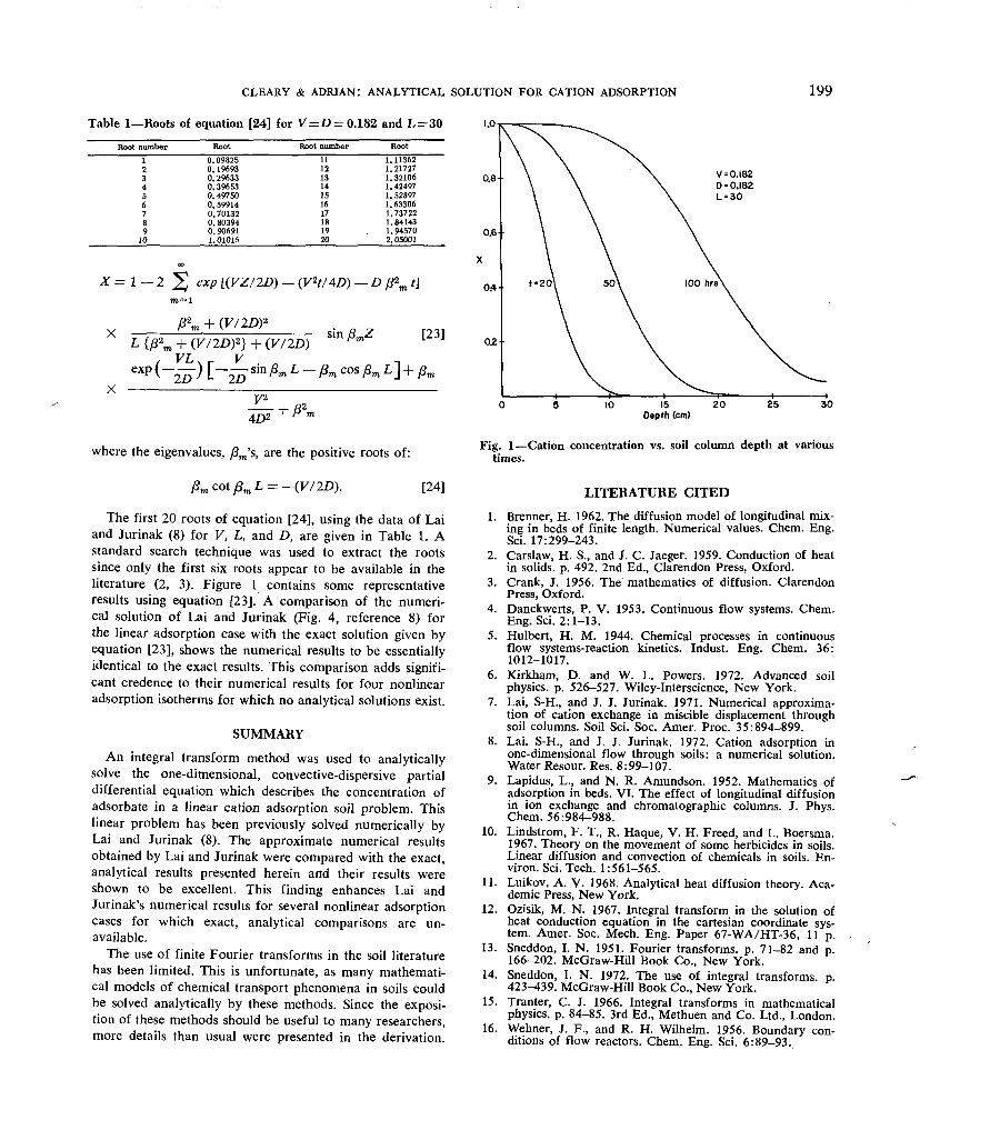
Table 1—Roots of equation [24] for V=D = 0.182 and L = 30Root number

123456789

10

Root0.098250. 196930. 296330.396530.497500. 599140.701320. 803940. 906911.01016

Root number11121314151617181920

Root1.113621.217271.321061.424971.528971.633061.737221.841431.945702.05001

X = I — 2 ̂ exp [(VZ/2D) — (V2t/4D) — D /?2m t]

m=l

Pm + (V/2DYX

X

sin /?mZL {pz

m + (K/2D)2} + (V/2D)/ VL. r V -.

CXP V~™ ) [~™ Sfn &» L - A» COS A» L] + &

[23]

2D 2DV*

4D2 + j82

where the eigenvalues, /6m's, are the positive roots of:

pncot/3nL = ~(V/2D). [24]

The first 20 roots of equation [24], using the data of Laiand Jurinak (8) for V, L, and D, are given in Table 1. Astandard search technique was used to extract the rootssince only the first six roots appear to be available in theliterature (2, 3). Figure 1 contains some representativeresults using equation [23]. A comparison of the numeri-cal solution of Lai and Jurinak (Fig. 4, reference 8) forthe linear adsorption case with the exact solution given byequation [23], shows the numerical results to be essentiallyidentical to the exact results. This comparison adds signifi-cant credence to their numerical results for four nonlinearadsorption isotherms for which no analytical solutions exist.

SUMMARYAn integral transform method was used to analytically

solve the one-dimensional, convective-dispersive partialdifferential equation which describes the concentration ofadsorbate in a linear cation adsorption soil problem. Thislinear problem has been previously solved numerically byLai and Jurinak (8). The approximate numerical resultsobtained by Lai and Jurinak were compared with the exact,analytical results presented herein and their results wereshown to be excellent. This finding enhances Lai andJurinak's numerical results for several nonlinear adsorptioncases for which exact, analytical comparisons are un-available.

The use of finite Fourier transforms in the soil literaturehas been limited. This is unfortunate, as many mathemati-cal models of chemical transport phenomena in soils couldbe solved analytically by these methods. Since the exposi-tion of these methods should be useful to many researchers,more details than usual were presented in the derivation.

V =0.1820 = 0.182L = 30

15 20Depth (cm)

Fig. 1—Cation concentration vs. soil column depth at varioustimes.