Analytical/Numerical Modelling of Two Parallel Robots as ... · the direct and inverse kinematics and dynamics had to ... The Parallel Robot 3SPS-1S Serial manipulators have some

Journal of Control Science and Engineering 2 (2015) 64-78 doi:10.17265/2328-2231/2015.02.002

Analytical/Numerical Modelling of Two Parallel Robots

as Laser Calibration Instruments Controlled by

Classical/Intelligent Schemes

Ricardo Zavala-Yoe1, Ricardo A. Ramirez-Mendoza1, Daniel Chaparro-Altamirano2 and Javier Ruiz-Garcia1

1. Tecnologico de Monterrey, Escuela de Ingenieríay Ciencias, Calle del Puente 222, Ejidos de Huipulco 14380, Mexico City

2. Computer Science Department, Columbia University, New York, USA

Abstract: Industrial metrology deals with measurements in production environment. It concerns calibration procedures as well as control of measurement processes. Measuring devices have been evolving from manual theodolites, electronic theodolites, robotic total stations, to a relatively new kind of laser-based systems known as laser trackers. Laser trackers are 3D coordinate measuring devices that accurately measure large (and relatively distant) objects by computing spatial coordinates of optical targets held against those objects. In addition, laser trackers are used to align truthfully large mechanical parts. However, such aligning can be done in moving parts, for instance during robot calibration in a welding line. In this case, serial robots are controlled in order to keep a prescribed trajectory to accomplish its task properly. Nevertheless, in spite of a good control algorithm design, as time goes by, deviations appear and a calibration process is necessary. It is well known that laser tracker systems are produced by very well established enterprises but their laser products may result expensive for some (small) industries. We offer two parallel robot-based laser tracker systems models whose implementation would result cheaper than sophisticated laser devices and takes advantage of the parallel robot bondages as accuracy and high payload. The types of parallel robots evaluated were 3-SPS-1-S and 6-PUS. Modelling of the parallel robots was done by analytical and numerical techniques. The latter includes classical and artificial intelligence-based algorithms. The control performance was evaluated between classical and intelligent controllers. Key words: Parallel robots, laser calibration, classical and al-controllers.

1. Introduction

The laser tracker measures 3D coordinates by

tracking a laser beam to a retro-reflective target held

in contact with the object of interest. They determine

three dimensional coordinates of a point by measuring

two orthogonal angles (azimuth and elevation) and a

distance to a corner cube reflector; typically a SMR

(spherically mounted retro-reflector). These balls

work as interface between the optical measurement

from the tracker and moving system [1, 7].

In this work we propose to use a couple of parallel

robots, a 3-SPS-1-S and a 6-PUS to implement a laser

tracker in calibration mode for a serial robot in a

welding line. In such a process, serial manipulators Corresponding author: Ricardo Zavala-Yoe, Ph.D., research

fields: modeling, nonlinear control, robotics. E-mail: [email protected].

need to be readjusted as time goes by. This

readjustment is done by tracking of the serial robot

position trajectory. Certain smooth path (a sinusoid

for instance) is fed to the serial manipulator in order to

be followed by a calibration device (the laser tracker).

We propose to simulate this calibration process by

coupling the dynamics of the arm with the parallel

robots’ one. So, the serial manipulator will move

following certain trajectory and the parallel robot in

turn has to track this trajectory in order to determine if

the serial robot is still calibrated. In order to

accomplish this task, both parallel robots will be

evaluated to determine which one tracks better the

serial arm.

In numerical simulations, we assume that an SMR

is placed at the far end of the welding robot. Once that

this robot starts moving following a reference signal

D DAVID PUBLISHING

Analytical/Numerical Modelling of Two Parallel Robots as Laser Calibration Instruments Controlled by Classical/Intelligent Schemes

65

(simulating the welding process) the laser tracker

(mounted in the parallel robot in turn) tracks the robot

arm trajectory directing its laser beam to the SMR

positioned at the welding arm (Fig. 1). Nevertheless,

we consider a more realistic situation of the latter by

adding a vibration on the floor (disturbance) as a

result of other machines work effects (section two).

In order to implement a set of controllers for this,

the direct and inverse kinematics and dynamics had to

be determined. For the former, classical and AI

(Artificial Intelligence)-based algorithms (GA

(Genetic Algorithms) and ANN (Artificial Neural

Networks)) were developed. The latter was useful to

design the control laws.

The control laws have two kinds: classical (no

AI-based) but linear and non-linear schemes as well as

intelligent controllers. The former is represented by a

PID (Proportional Integral Derivative) controller (linear

case) and by a SMC (Sliding Mode Control) algorithm

(non-linear case). The latter, by a F-PD (Fuzzy

Proportional Derivative) controller and by a FSM

(Fuzzy Sliding Mode) controller. For sake of clarity,

some results here were taken from Refs. [2, 3, 8, 9, 17].

All the algorithms were run in MATLAB/Simulink.

Section two describes the interaction between the

serial arm and the parallel robot in turn.

Section three concerns the theoretical development

of the kinematics and dynamics of the 3-SPS-1S

manipulator as well as part four does the same for

the 6-PUS robot. Next, the results of the performance

evaluation of both parallel robots are given in

sections five and six. Finally, conclusions are

discussed in part seven.

2. Modelling the Parallel-Serial Robots Interaction

In this work, both parallel robots-based laser tracker

systems are used to assess a serial arm tracking

performance. As it was explained in abstract, the serial

manipulator suffers deviations from its reference

signal as time goes by. Naturally, the serial arm works

in industrial environment, which implies that its

tracking control algorithm can deal with disturbances

(vibrations) produced in the welding line. This fact

implies that the parallel robot also has to deal with

these disturbances in order to warrant a good deviation

test for the serial manipulator. The performance of

both robots, the 3-SPS-1S and the 6-PUS were tested

and reported here. The pair of robots will track the

serial one. In order to accomplish this goal, two

classical controllers were evaluated for each parallel

robot model: a linear one, a PID controller and a

non-linear one, a SMC. Later, two fuzzy logic

controllers were tested: a F-PD controller and a

F-SMC, which is actually a fuzzy sliding mode

proportional controller. See sections five and six. The

persistent perturbation p(t) which models the vibration

of other machines and which affects our laser tracker

performance is defined as p(t) = 0.1sin(2π(5)t)

because it is assumed that the serial arm moves

according to a reference signal given by r(t) =

0.5sin(2π(0.5)t). So, the disturbance frequency is ten

times bigger than the reference’s one. Although the

serial robot is an industrial arm with six degrees of

Fig. 1 Interaction between two different kinds of robots via AI and classical control in the presence of disturbances.


66

freedom, for the purposes of tracking calibration it

will move as a three degrees of freedom robot. The

base will rotate from left to right, and by keeping

fixed three joints, the equivalent upper structure will

be a two degrees of freedom serial robot (Fig. 1). The

latter structure will develop an up-down sinusoid

motion for its end effector. This equivalent two

degrees of freedom serial robot is a well known

nonlinear dynamical system [10] which was modeled,

controlled (by a F-SMC) and simulated in Ref. [15].

As this serial arm exhibited a very good performance

with the above mentioned controller [15], for the

current experiment its output position was recorded in

Simulink. This signal was used as the reference signal

for the parallel robot, modelling in this way that the

laser beam mounted on the parallel robot is linked to

SMR on the serial robot’s end effector. As a

consequence, the parallel robot (laser tracker) will

have to move considering its Euler angles (section

three) according to the following considerations: ω =

0.01, φ is the signal received from the serial

manipulator and which has to approximate φ =

0.5sin(2π(0.5)t), and ψ = 3sat(t), t ≥ 0 for tracking.

The latter provide a side to side swiping in order to

track the y-axis motions of the serial arm and φ tracks

the sinusoid signal done by the serial robot. This

simulation was developed in MATLAB/Simulink

environment. For regulation purposes, the Euler

angles references are chosen to be ω = 0.01, φ = 1(t),

and ψ = 3sat(t), t ≥ 0, where 1(t) is a unit step. Finally,

ω = 0.01 keeps a small enough fixed ω ≠ 0 away from

its singularity.

3. The Parallel Robot 3SPS-1S

Serial manipulators have some drawbacks with

respect to parallel robots. More accuracy, higher load

capacity/robot mass ratio and more rigidity are just a

few [6, 13]. Recall that a parallel robot consists of a

fixed base connected by limbs to an (upper) moving

platform (the end effector). The limbs are conformed

by links and joints. So, parallel robots denominations

come from their link structure. For instance, 3-SPS-1S

means that the robot has three identical limbs with

spherical (S) joints at the extremes and a prismatic

joint (P) in the middle plus one passive (non actuated)

joint in the middle of the end effector whose extremes

are also spherical (1S).

Cui and Zhang propose a special type of the robot

3-SPS-1S [4]. Such architecture is shown in Fig. 2. It

has three identical legs, made of two bodies, linked by

an actuated prismatic joint. The legs are attached to

the platform and the base by spherical joints. It is

assumed that the platform and the base are circular,

with radii pr and br respectively, and that the

spherical joints of the legs are located along these

circumferences. There is also a central passive leg that

connects the center of the base to the center of the

platform using a spherical joint. There are two

coordinate systems. The general coordinate system xyz

is located at the center of the base (point O), and the

coordinate system of the platform uvw with origin on

point P is located at the center of the spherical joint of

the central leg. The orientation of the platform is given

in terms of the Euler angles which are three angles

introduced by Euler to describe the orientation of a

rigid body [11, 13]. The central constraining leg of the

mechanism increases the stiffness of the system and

forces the manipulator to have three pure rotation

degrees of freedom.

3.1 Classical and AI-Based Algorithms to Determine

the Workspace

As a result of such analytical complexity of the

equations which describe the workspace manipulator,

it is not possible to give a closed solution for the

workspace. Hence, numerical algorithms are required.

For this manipulator, two kinds of algorithms were

developed in Ref. [2]. The first type does not use

artificial intelligence-based programs and the other

one does.

The former is based in five algorithms which look

for the right points in the 3D space while the


67

Fig. 2 Model of the 3SPS-1S parallel wrist and corresponding Euler angles for the end effector (moving platform).

following conditions are checked: rightness of limbs

length, avoiding collision among limbs, and restriction

in the Euler angles. The resulting workspace is shown

in Fig. 3, left panel. However, as it can be seen in Fig.

3, the workspace looks small. So, a GA optimization

was included to find the biggest workspace subject to

the robot’s dimensions/mobility constraints [2]. It is

known that the 3-SPS-1S parallel wrist is

characterized by its lack of a big workspace; therefore,

optimizing the parameters of the robot in order to

maximize the workspace is very important.

Nevertheless, it is also important for the manipulator

to have its parameters br , pr and h as close as

possible to a set of desired parameters, mainly because

many times there are size limitations in the location

where the manipulator is to be placed. This method

tries to maximize the workspace and at the same time,

keep the robot parameters as close as possible to a set

of desired parameters. The resulting optimized

workspace can be seen in Fig. 3. See details in Ref.

[2].

Linked with determination of the workspace is the

computation of singularities which were calculated

numerically in Ref. [2] by an algorithm which checks

the Jacobian matrix of the manipulator. Singularities

appear at ω∈ IR, φ = ψ = 0, where IR is the set of all

real numbers.

3.2 Inverse Kinematics

It was chosen to solve the inverse kinematics first

because it is easier for parallel robots than for their

serial counterparts. Recall that the inverse kinematics

problem considers that a desired position is known but

the limb variables (links length) have to be computed.

So, given the Euler angles ω, φ, ψ, the length of the

limbs id has to be calculated (Fig. 2). The 3SPS-1S

inverse kinematics problem was also solved in Ref. [2]

and is given by the following expression:

.3,2,1,

222

ibbb

hbababd

Tziyixiii

BB

A

ziyiyixixii

bbR(1)

Fig. 3 Left: Workspace computed with conventional algorithms (no GA). Right: Optimized workspace determined via GA.


68

where, Tyixi aa 0,,ia be the vector from origin O to point iA in the xyz system, ib

B the vector from

origin P to point iB in the rotating system uvw,

Th,0,0P , the vector between points O and P.

Upper indices imply change of frame reference by

rotation matrices. They are not included here but they

were well explained in Refs. [3, 13].

3.3 Direct Kinematics via ANN

The direct or forward kinematics problem is to

deduce the orientation of the moving platform (ω, φ, ψ)

when the limbs length id , i = 1, 2, 3 are known (Eq.

(1) and Fig. 2). A numerical/geometric method was

proposed in Ref. [2] in order to solve the direct

kinematics problem. Nevertheless, such algorithm

produced more than one solution. In order to find only

one solution, an algorithm consisting of an ANN and a

Newton-Raphson method was implemented in Ref. [2].

Roughly speaking, a system defined by Eqs. (1) and (2)

has to be solved:

ccsscscsccss

scsssscsscsc

ssccc

R

b

b

b

R

b

b

b

BA

z

y

x

BA

z

y

x

i

i

i

i

i

i

, (2)

Obviously this system of equations does not have

analytical solution and a numerical method is

necessary. The method chosen was Newton-Raphson

but this algorithm requires to provide an initial value

close enough to the actual solution but such solution is

unknown of the system. In order to find such

approximate initial value an ANN was proposed.

For any given length of the limbs and initial

position of the platform, it is possible to find an

approximate solution to the direct kinematics using

the trained ANN. Once the approximate solution is

found, Eq. (1) can be written three times (one for each

limb) and the system of three non-linear equations can

be solved using the Newton-Raphson’s method. A

validation set consisting of 100 positions was used to

check the method. The result error between the two

trajectories was negligible.

3.4 Dynamics

In dynamics there also exist the inverse and the

direct problems. The direct dynamics problem

concerns to find the trajectory (and time derivatives)

of the platform given the forces or torques in the

actuators. On the other hand, the inverse dynamics

problem determine the required forces or torques to

get a given trajectory [6, 13]. In Ref. [3] the direct and

inverse dynamics models were obtained. The direct

model is linked with (open or closed loop) simulations

purposes, i.e., a state space representation

),( uxfx , where, x is the state variable and u is

the control signal. The inverse dynamics is concerned

with the controller design (recall Lyapunov-based

design [10]). The computation of a control law will

provide the right forces/torques to accomplish a given

task, so in order to simulate the closed loop system,

the direct dynamics of the manipulator is needed. The

work done in Ref. [3] provides further details about

the following direct dynamics model.

221

11 VTτJVTx Tp (3)

where,

pIT 1 (4)

ppp ωIωT 2 (5)

*1 ii bU (6)

ippi bωωU 2 (7)

3

11

221 **

iiii

i

i

dUsb

JV (8)

3

12

222 **

iiii

i

i

dUsb

JV (9)

In addition, pI is the inertia matrix of the platform,


69

pω the angular velocity of the platform, ib the

vector going from point P to point iB , is is the unit

vector pointing from iA to iB and id is the length

of the ith leg, i = 1, 2, 3, [3, 6, 12]. The inertial effect

caused by the laser unit mass was considered by

increasing the moving platform mass, altering global

inertial effects in Eq. (3). So, the parallel robot plus

the laser beam unit, i.e., the laser tracker system

considered here is represented by Eq. (3). The latter

will be the plant controlled by AI algorithms and by

classical control schemes according to the explanation

given in section one. The inverse dynamics was

obtained in Ref. [3].

4. The 6-PUS Parallel Robot

The 6-PUS architecture is a mechanism which

consists of the fixed platform, the end effector (moving

platform) and six limbs with the same structure. Every

limb is conformed by a prismatic joint (P) and a

universal joint (U) in the base, plus a spherical

articulation (S) at the end of the branch (Fig. 4).

4.1 Inverse Kinematics

It is well known that solving the inverse kinematics

problem for a parallel robot is relatively easy. In Fig. 5,

it can be deduced that the joint displacements are

given by:

2 2 22 2 2 2

1,...,6; { , , }.

T Tij j ij ij j ij ij i i i i i id p b a p b a r

i j x y z

p b a p b a b a (10)

4.2 Numerical Computation of the Workspace

The singularities and workspace for this

manipulator were solved by programming several

algorithms which considered the geometry and

actuators constraints. Thus, the end effector jacobian

matrix xJ and the joint variables jacobian matrix qJ

were obtained computationally in Ref. [9], Fig. 6.

4.3 Direct Kinematics

The direct kinematics was solved numerically in

Ref. [9]. An algorithm referred to as arcs method is

deduced and programmed. It is also explained there

how an improved design of the circular end effector

was developed. The former rounded design was

changed by a triangular shape which resulted to

behave better.

4.4 Dynamics

The direct and inverse dynamics problems for this

robot were solved in Ref. [8]. However, the analytic

expression for the inverse dynamics is more

complicated for the 6-PUS robot than for the

3-SPS-1S robot. The reason is that there are three

forces involved and only one is known. See details in

the above mentioned reference. In contrast, the direct

dynamics representation is less complicated for this

6-PUS robot than the one for the 3-SPS-1S

manipulator. Such model is given below:

HGτJGW 11 T (11)

where, TωυW and υ, ω are the translational

velocity and the angular acceleration of the center of

gravity of the end effector respectively. In addition:

2 ,* *

(

)

m m

m m

m

m

eG

e I e

ω e) ω gH

ω Iω e * (ω e) ω g

(12)

Fig. 4 6-PUS robot limbs and articulations.


70

Fig. 5 6-PUS robot geometry and rendered model. The Euler angles are defined in the same way as for 3-SPS-1S robot (in Fig. 2).

Fig. 6 6-PUS robot workspace is obtained by solving

numerically det( qJ ) = 0.

Fig. 7 Final design of the 6-PUS robot.

0

0

e-0

* is that ,*

12

13

23

ee

ee

e

exexe (13)

and a is an arbitrary 3 x 1 vector. q1x JJJ is a

Jacobian matrix which relates displacements of the

platform with displacements of the actuators and

represents the forces applied to the actuators of each

limb [3, 8].

5. The Case of the 3-SPS-1S Robot

5.1 Closed Loop System

As it was mentioned before, two classical (crisp)

controllers are tested here in terms of performance.

Later, they will be compared with their AI-based

counterparts. The general control loop used in this

work is shown in Fig. 8 where the controller will be

generic and will be either classical or intelligent. It is

remarkable that the blocks are very complex and

details are omitted. Note for instance that the Euler

angles have to be transformed to actuator variables by

means of the inverse kinematics blocks (Fig. 8).

Although equations are mathematically enough to

describe a dynamical system, the gap between models

and numerical implementation is huge [16, 17]. It is

remarkable that in Fig. 8 each block contains many

sub blocks and MATLAB scripts. They contain the

equations described through all the paper.

5.2 Regulation Case

As explained in Ref. [2], three Euler angles

references were chosen in order to assess two classical


71

Fig. 8 Generic closed loop for all the control schemes.

controllers, a linear PID controller and a non-linear

controller; a SMC. Both performances were simulated

and explained below.

5.2.1 Linear PID Controller

A PID controller was implemented in the model

environment described above. Recall that a

PID-control law is defined by

dtxxKxKu DP~~~ (14)

where, μ is the control law, xxx d ~ is the error

of the closed loop system, dx is a desired variable

(reference), and x is an actual variable to be

compared with the reference. In this case the poor

nature of the linear PID controller could not deal with

the complex and perturbed dynamics of the parallel robot. Angles and could not be regulated and

the performance presented by was quite poor,

reaching the unit reference after seven seconds. The

figure is not shown.

5.2.2 Nonlinear Controller: SMC

It is well known that a sliding mode regime allows

asymptotic stability and asymptotic tracking via

Lyapunov theory [10]. Such regime is accomplished

by a suitable controller designed in terms of the

sliding variable s which allows the state variables of

the dynamical model to converge to an invariant set

referred to as sliding hyperplane. The sliding variable

s and its corresponding time derivative are given by

the following equations [10]:

0,~,~~ xxxxxs d (15)

xxs ~~ (16) where, dx is the desired variable (reference to

follow) and x is the interest variable, a state variable

or a generalized coordinate. The SMC could regulate

the laser tracker proposed in a relatively good way

needs three seconds to achieve the goal (Fig. 9).

Obviously, the complexity of this controller helped to

regulate the parallel robot outputs.

5.3 Tracking Case


The reference angles for tracking were explained in

section two. The resulting positions of the perturbed

laser tracker were given in Ref. [17]. It was clear that

the PID can deal with neither disturbances nor the

parallel robot dynamics.

5.3.2 Nonlinear Control: SMC

It was mentioned that Eq. (3) was referred to as

direct or forward dynamics. In this section, it is more


72

Fig. 9 Reference and output Euler angles of the parallel robot controlled by a SMC.

convenient to consider its dual, i.e., the inverse

dynamics. The inverse dynamics model is more

suitable to design nonlinear controllers as the SMC.

Renaming 1VTM 1p , 2VTK 2p , τJu T ,

where, p stands for platform, Eq. (3) can be written as

Eq. (17):

uKxM ppp (17)

In the sense of [10], the control law which can deal

with the above mentioned disturbance in sliding mode

regime was designed as follows:

( ) ) ( ),

, , 0

p t sat

k k

p pd p p pu (M x K M Λx K s

Λ I K I

(18)

where, sat(s) stands for saturation function of s and I

is the identity matrix. The last summand in the latter

equation is a compensation term which achieves the

sliding regime. The closed loop system results from

substituting Eq. (18) in Eq. (17) yielding:

)()(( sKI)KIsM p sattp (19)

By means of Lyapunov theory stability and tracking

are achieved [10, 15]. Consult the corresponding

perturbed outputs in Ref. [17].

It is noteworthy mention that although SMC is very

robust and in general provide good close loop

performance, its computation may take long time and

frequently ends up with numerical stiff problems as a

consequence of the highly non-linear closed loop, i.e.,

plant plus controller. The SMC parameters used here

were 33.0 and 1k .

5.4 Artificial Intelligence-Based Controllers

Next, the AI version of the latter PID and SMC

controllers are assessed here. It is well known that

AI-based controllers have good performance in

difficult situations as partially known models of a

plant, complex (nonlinear) systems, etc. [5].

5.4.1 Regulation Case

For comparison purposes, two AI-based controllers,

analog to their classical partners were designed in this

section. First, a fuzzy proportional derivative

controller was implemented and later, a fuzzy sliding

mode controller was tested. Their performance and

simulation results are explained next.

5.4.2 Fuzzy Proportional Derivative Controller

This controller has two fuzzy inputs and one fuzzy

output. This controller ended up to be a relatively

good regulator for this set of references. It seems that

the fuzzy conversion of the crisp signals and the

complete fuzzy signal processing helped to deal with

this regulation problem.

5.4.3 Fuzzy Sliding Mode Controller

In contrast to F-PDC, the F-SMC was not able


73

enough to regulate the laser tracker outputs as desired.

Although this controller takes advantages of its fuzzy

part, this one is not enough to deal with the complex

dynamics of the parallel robot plus the perturbed input.

In this case, ω diverged, and although ψ and φ did not

diverged, their performance was quite poor.

5.5 Tracking Case

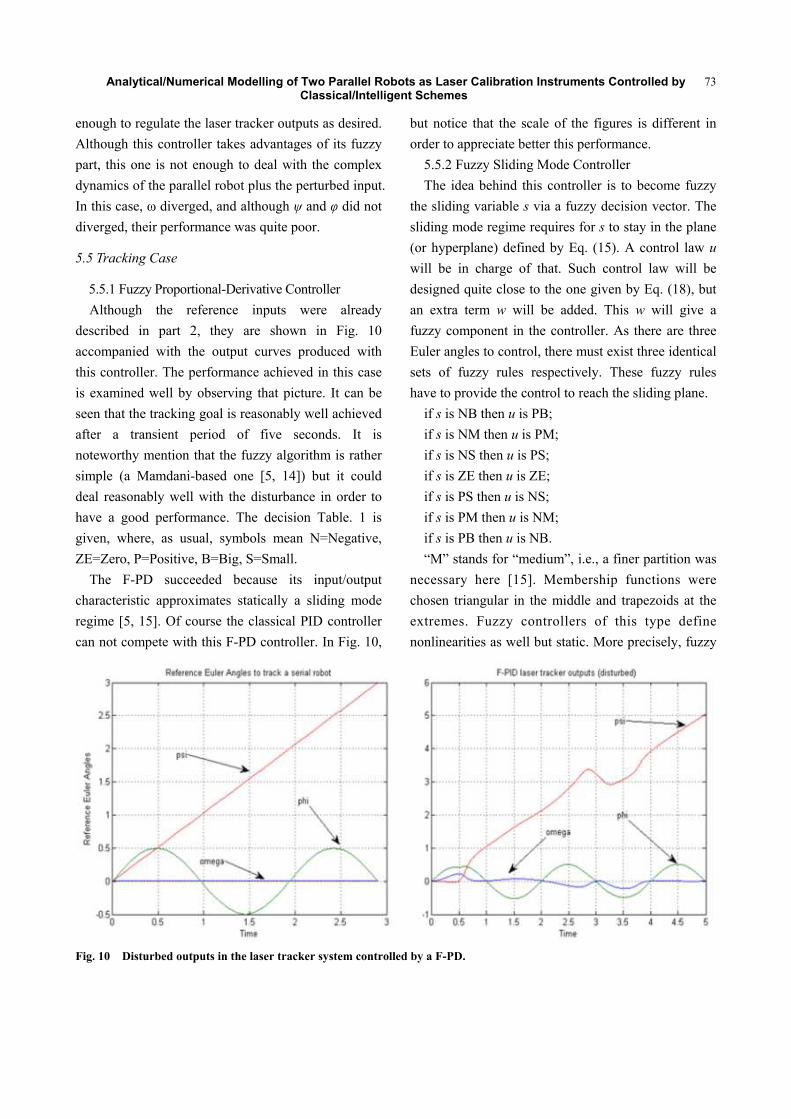
5.5.1 Fuzzy Proportional-Derivative Controller

Although the reference inputs were already

described in part 2, they are shown in Fig. 10

accompanied with the output curves produced with

this controller. The performance achieved in this case

is examined well by observing that picture. It can be

seen that the tracking goal is reasonably well achieved

after a transient period of five seconds. It is

noteworthy mention that the fuzzy algorithm is rather

simple (a Mamdani-based one [5, 14]) but it could

deal reasonably well with the disturbance in order to

have a good performance. The decision Table. 1 is

given, where, as usual, symbols mean N=Negative,

ZE=Zero, P=Positive, B=Big, S=Small.

The F-PD succeeded because its input/output

characteristic approximates statically a sliding mode

regime [5, 15]. Of course the classical PID controller

can not compete with this F-PD controller. In Fig. 10,

but notice that the scale of the figures is different in

order to appreciate better this performance.

5.5.2 Fuzzy Sliding Mode Controller

The idea behind this controller is to become fuzzy

the sliding variable s via a fuzzy decision vector. The

sliding mode regime requires for s to stay in the plane

(or hyperplane) defined by Eq. (15). A control law u

will be in charge of that. Such control law will be

designed quite close to the one given by Eq. (18), but

an extra term w will be added. This w will give a

fuzzy component in the controller. As there are three

Euler angles to control, there must exist three identical

sets of fuzzy rules respectively. These fuzzy rules

have to provide the control to reach the sliding plane.

if s is NB then u is PB;

if s is NM then u is PM;

if s is NS then u is PS;

if s is ZE then u is ZE;

if s is PS then u is NS;

if s is PM then u is NM;

if s is PB then u is NB.

“M” stands for “medium”, i.e., a finer partition was

necessary here [15]. Membership functions were

chosen triangular in the middle and trapezoids at the

extremes. Fuzzy controllers of this type define

nonlinearities as well but static. More precisely, fuzzy

Fig. 10 Disturbed outputs in the laser tracker system controlled by a F-PD.


74

Table 1 Fuzzy Rules for the F-PD.

xx ~~ NB NS ZE PS PB

NB NB NB NB NS ZE

NS NB NB NS ZE PS

ZE NB NS ZE PS PB

PS NS ZE PS PB PB

PB ZE PS PB PB PB

rules surfaces are nonlinear static (memoryless)

bounded sector nonlinearities [5, 15]. The

input-output surface (actually a curve) for the set of

rules shown above is a distorted straight line. That is

why this fuzzy control is only proportional. Now it is

necessary to define the sliding control law as it was

done in Eq. (18). Adding an extra compensation term

w to Eq. (18) yields Eq. (20):

0,,

,)()~)(

kk

sattp

IKIΛ

wsKxΛMKx(Mu ppppdp

(20)

Again, by Lyapunov theory a positive definite

function was chosen in such a way that its derivative

can be negative definite in order to warrant stability

and tracking (see section 5.3.2 and Refs. [10, 15]).

In this case the performance obtained was poor

with respect to the reference signal. The reason is

that the fuzzy decision rules have one input and one

output and this construction is not enough to deal with

this problem. Lyapunov theory indicates that the

control law given by Eq. (20) will work properly as

long as the variable w provides enough energy. This

is not the case for this system. Note that the set of

rules of the F-SMC defines only a proportional

sliding mode controller. Nevertheless a F-SMC has

achieved a good performance for a simpler nonlinear

dynamics, the robot described in Ref. [15]. Summing

up, for regulation and tracking, the F-PD controller

ended up to be the best. The second place corresponds

to the SMC.

6 The Case of the 6-PUS Robot

6.1 Closed Loop System

The closed loop system for this robot corresponds

also to the one shown in Fig. 8. It is noteworthy

mention that the general performance of this

manipulator was a bit worse than the one achieved by

the 3-SPS-1S manipulator. One has to reflect that the

central limb of the 3-SPS-1S is a clear advantage

because that link helps to keep stability and tracking.

6.2 Regulation Case


This controller’s performance resulted to be very

poor as a result of the simplicity of the PID controller

with respect to the complexity of the 6-PUS

robot. The output responses are not shown for this

reason.

6.2.2 Nonlinear Control: Sliding Mode Controller

The inverse model was used here to design the

SMC for this robot. The stability analysis is similar to

the one done for the 3-SPS-1-S and it will not be

repeated here (see section 5.3.2). In contrast with the

PID controller, the SMC behaved better although with

some difficulties before the first six seconds of

simulation time. The parameters used in this case were

5.0 and 1k .

6.3 Tracking: Linear and Non-linear Cases

Similarly to the 3-SPS-1S the tracking task was not

accomplished successfully neither by the PID

controller nor by the SMC. Recall that the 6-PUS does

not possess a central passive limb as the 3-SPS-1S.

This fact implies a drawback for the 6-PUS in

regulation and tracking. As a result of this, these

curves are not included.

6.4 AI-Based Controllers: F-PDC and F-SMC

The set of controllers used in the 3-SPS-1S robot

were applied to the 6-PUS as well. For the case of the

Fuzzy Proportional Derivative Controller (F-PDC),

the decision table changed with respect to the one

used for the 3-SPS-1S as shown in Table 2. Observe

the region around ZE which needs more control effort

as the 3-SPS-1S controller.


75

Fig. 11 Regulation response of the 6-PUS platform, compared with Fig. 9.

Table 2 Fuzzy rules for the F-PD.

xx ~~ NB NS ZE PS PB

NB NB NB NB NS ZE

NS NB NS NS ZE PS

ZE NB NS ZE PB PB

PS NS ZE PS PS PB

PB ZE PS PB PB PB

The corresponding output is given in Fig. 12.

Notice how the ψ angle can not track well the

saturation reference compared with Fig. 10.

The F-SMC was described in 5.5.2. There were two

changes in the decision vector. The consequent in rule

number three became PB instead of PS. Analogously

happened in rule five. The consequent became NB

instead of NS. The Lyapunov analysis was done here

in the same way as in section 5.5.2. The resultant

performance was similar to the case of the 3-SPS-1S

and figures are not provided. In general, the performance

showed by the 6-PUS robot was a bit worse than the

one displayed by the 3-SPS-1S. One reason is that the

central leg in the latter robot helps to provide stability,

especially in tracking tasks. Nevertheless, an extra set

of tracking tasks was designed for this robot in order

to redeem his performance.

6.4.1 Extra Tracking Tasks

Three further tests were done in this case. One is a

Fig. 12 Tracking response of the 6-PUS platform due to a F-PD controller.


76

circular trajectory on the plane x-y keeping height

(z-axis) constant at 5 cm. The output position

trajectory of the platform is shown in Fig. 13 with the

forces required in the actuators to produce such

oscillatory path.

An animation for the 6-PUS model was created in

MATLAB in order to illustrate how the robot moves.

The red circles on the platform indicate the oscillatory

motion of the end effector, showed in Fig. 14.

The second tracking test was done enhancing the

latter scenario. A 3D swinging was performed by the

6-PUS robot. Similarly to the latter case, the platform

position is given for the three axis as well as the forces

required in the actuators, in Fig. 15.

Fig. 13 An oscillatory motion of the platform on the x-y plane produces the following output position with the

corresponding actuators forces i, i = 1,..., 6.

Fig. 14 Fluctuating 3D motion of the platform with constant height.

Fig. 15 A 3D oscillatory motion of the 6-PUS platform. The corresponding actuators forces , i = 1,..., 6 are also given.


77

Fig. 16 MATLAB model which illustrates a swinging 3D trajectory of the platform with constant height.

Fig. 17 The parallel robot tracks a letter M trajectory. The joint distances computed are here.

A frame of an animation for this case is shown in

Fig. 16 from two perspectives.

The third tracking test was developed in a more

difficult trajectory. In this case the parallel

manipulator had to follow a letter M path created by

the serial arm. The results for the actuators length are

given in Fig. 17.

7. Conclusions

Two types of parallel robots were evaluated to be

used as laser tracker systems, a 3-SPS-1-S and a

6-PUS. In general, considering the classical and

AI-based controllers, the performance obtained by the

former was a little bit better than the latter as a result

of the central extra passive link which help to stabilize

the end effector. Nevertheless, it is well known that

parallel robots are very difficult to deal with, either

modelling them or simulating them. Moreover, to

design a satisfactory control law is rather challenging.

But if in addition to the laser tracker models proposed,

an interacting dynamics with an extra serial robot in a

perturbed environment are considered, the global

scenario results quite complicated to deal with.

Numerical stiffness, algebraic loops come into picture

due to the highly non-linear interaction in the whole

system.

References

[1] Burge, J., Peng, S., and Zobrist, T. 2007. “Use of a Commercial Laser Tracker for Optical Alignment.” In Proceedings of the SPIE Optical System Alignment and Tolerancing, 1-12.

[2] Chaparro-Altamirano, D., Zavala-Yoe, R., and

Ramirez-Mendoza, R. 2013. “Kinematic and Workspace

Analysis of a Parallel Robot Used in Security

Applications.” In Proceedings of the IEEE International


78

Conference on Mechatronics, Electronics and Automotive

Engineering, Mexico.

[3] Chaparro-Altamirano, D., Zavala-Yoe, R., and Ramlrez-Mendoza, R. 2014. “Dynamics and Control of a 3SPS-1S Parallel Robot Used in Security Applications.” In Proceedings of the 21st International Symposium on Mathematical Theory of Networks and Systems, Groningen, Netherlands.

[4] Cui, G., and Zhang, Y. 2009. “Kinetostatic Modelling and Analysis of a New 3-DOF Parallel Manipulator.” In Proceedings of the IEEE International Conference on Computational Intelligence and Software Engineering, 1-4.

[5] Driankov, D., Hellendorn, H., and Reinfrank, M. 1996.

An Introduction to Fuzzy Control. Springer.

[6] Merlet, J. P. 2006. Parallel Robots. Solid Mechanics and

its Applications. Springer.

[7] Prenninger, J. P., Filz, K. M., Incze, M., and Gander, H.

1995. “Real-Time Contactless Measurement of Robot

Pose in Six Degrees of Freedom.” Measurment 14:

255-64.

[8] Ruiz-Garcia, J., Zavala-Yoe, R., Ramirez-Mendoza, R., and Chaparro-Altamirano, D. 2013. “Direct and Inverse Dynamic Modelling of a 6-PUS Parallel Robot.” In Proceedings of the IEEE International Conference on Mechatronics, Electronics and Automotive Engineering, Mexico.

[9] Ruiz-Garcia, J., Zavala-Yoe, R., Ramirez-Mendoza, R., and Chaparro-Altamirano, D. 2013. “Numerical-Geometric Method to Determine the Direct

Kinematics of a 6-PUS Parallel Robot.” In Proceedings of the IEEE International Conference on Mechatronics, Electronics and Automotive Engineering, Mexico.

[10] Slotine, J., and Li, W. 1991. Applied Nonlinear Control. Pearson Education.

[11] Tsai, L. W. 1996. “Kinematics of A Three-Dof Platform with Three Extensible Limbs.” In Recent Advances in Robot Kinematics, chap. 8: 401-10. Springer.

[12] Tsai, L. W. 1998. “Solving the Inverse Dynamics of Parallel Manipulators by the Principle of Virtual Work.” In Proceedings of the ASME Design Engineering Technology Conference, 451-7.

[13] Tsai, L. W. 1999. Robot Analysis: The Mechanics of Serial and Parallel Manipulators. John Wiley & Sons.

[14] Zadeh, L. A. 1965. “Fuzzy Sets.” Information and Control 8: 338-53.

[15] Zavala-Yoe, R. 1997. “Fuzzy Control of Second Order Vectorial Systems: L2 Stability.” In Proceedings of the European Control Conference, Belgium.

[16] Zavala-Yoe, R. 2008. “Modelling and Control of Dynamical Systems: Numerical Implementation in a Behavioral Framework.” Studies in Computational Intelligence. Springer.

[17] Zavala-Yoe, R., Chaparro-Altamirano, D., Ramirez-Mendoza, R. A. 2014. “Artificial Intelligence-Based Design of a Parallel Robot Used as a Laser Tracker System: Intelligent vs. Nonlinear Classical Controllers.” Lecture Notes in Computer Science: Nature-Inspired Computation and Machine Learning, 392-409.

Documents

Analytical/Numerical Modelling of Two Parallel Robots as ... · the direct and inverse kinematics and dynamics had to ... The Parallel Robot 3SPS-1S Serial manipulators have some