Analyzing Terrain and Surfaces - MicroImages, Inc

Analyzing Terrain and Surfaces

page 1

Tutorial

Analyzing Terrainand Surfaces

with

TNTmips®

TERRAIN

ANALYSIS


page 2

Before Getting StartedTopography profoundly influences many physical and biological processes andprovides the backdrop for human activities such as construction, transportation,communication, resource management, and recreation. Because of the variedways in which natural or manmade systems interact with landscapes, computeranalysis and modeling of terrain requires a number of specialized software tools.This booklet introduces a series of TNTmips® processes that allow you to ana-lyze elevation rasters and to model various types of interaction with terrain.

Prerequisite Skills This booklet assumes that you have completed the exercisesin the tutorials entitled Displaying Geospatial Data and TNT Product Concepts.Those exercises introduce essential skills and basic techniques that are not cov-ered again here. Please consult those booklets for any review you need.

Sample Data The exercises presented in this booklet use sample data that isdistributed with the TNT products. If you do not have access to a TNT productsDVD, you can download the data from MicroImages’ web site. In particular, thisbooklet uses sample files in the TERRAIN data collection. Be sure the sample datacollection has been installed on your hard drive so changes can be saved as youuse these objects in the following exercises.

More Documentation This booklet is intended only as an introduction to terrainand surface analysis. Details of the process can be found in a variety of tutorialbooklets, color plates, and Quick Guides, which are all available fromMicroImages’ web site (go to http://www.microimages.com/search to quicklysearch all available materials, or you can narrow your search to include onlytutorials or plates.

TNTmips® Pro and TNTmips Free TNTmips (the Map and Image ProcessingSystem) comes in three versions: the professional version of TNTmips (TNTmipsPro), the low-cost TNTmips Basic version, and the TNTmips Free version. Allversions run exactly the same code from the TNT products DVD and have nearlythe same features. If you did not purchase the professional version (which re-quires a software license key) or TNTmips Basic, then TNTmips operates inTNTmips Free mode. All the exercises can be completed in TNTmips Free usingthe sample geodata provided.

Randall B. Smith, Ph.D., 23 August 2013©MicroImages, Inc., 2001-2013

You can print or read this booklet in color from MicroImages’ Web site. TheWeb site is also your source for the newest tutorial booklets on other topics.You can download an installation guide, sample data, and the latest version ofTNTmips.

http://www.microimages.com


page 3

STEPSchoose Main / Displayfrom the TNTmips menu

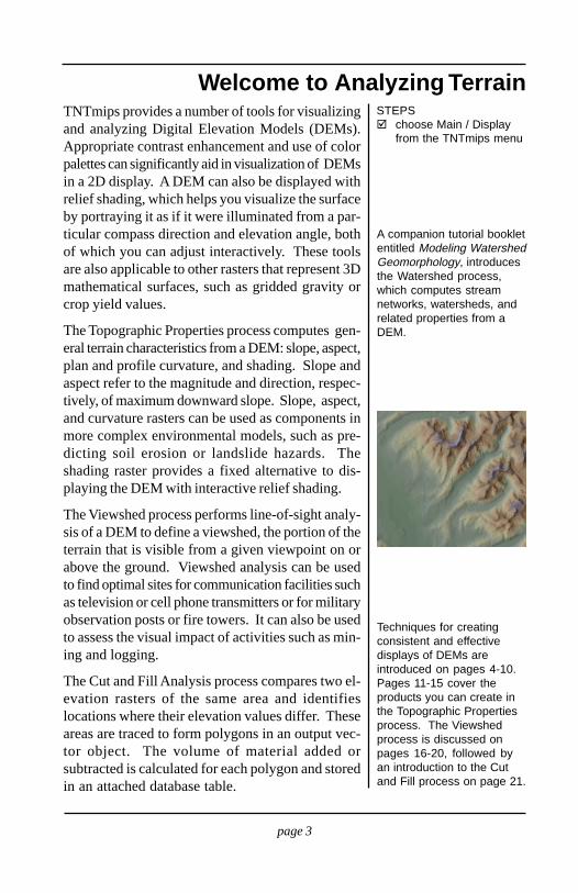
Welcome to Analyzing TerrainTNTmips provides a number of tools for visualizingand analyzing Digital Elevation Models (DEMs).Appropriate contrast enhancement and use of colorpalettes can significantly aid in visualization of DEMsin a 2D display. A DEM can also be displayed withrelief shading, which helps you visualize the surfaceby portraying it as if it were illuminated from a par-ticular compass direction and elevation angle, bothof which you can adjust interactively. These toolsare also applicable to other rasters that represent 3Dmathematical surfaces, such as gridded gravity orcrop yield values.

The Topographic Properties process computes gen-eral terrain characteristics from a DEM: slope, aspect,plan and profile curvature, and shading. Slope andaspect refer to the magnitude and direction, respec-tively, of maximum downward slope. Slope, aspect,and curvature rasters can be used as components inmore complex environmental models, such as pre-dicting soil erosion or landslide hazards. Theshading raster provides a fixed alternative to dis-playing the DEM with interactive relief shading.

The Viewshed process performs line-of-sight analy-sis of a DEM to define a viewshed, the portion of theterrain that is visible from a given viewpoint on orabove the ground. Viewshed analysis can be usedto find optimal sites for communication facilities suchas television or cell phone transmitters or for militaryobservation posts or fire towers. It can also be usedto assess the visual impact of activities such as min-ing and logging.

The Cut and Fill Analysis process compares two el-evation rasters of the same area and identifieslocations where their elevation values differ. Theseareas are traced to form polygons in an output vec-tor object. The volume of material added orsubtracted is calculated for each polygon and storedin an attached database table.

A companion tutorial bookletentitled Modeling WatershedGeomorphology, introducesthe Watershed process,which computes streamnetworks, watersheds, andrelated properties from aDEM.

Techniques for creatingconsistent and effectivedisplays of DEMs areintroduced on pages 4-10.Pages 11-15 cover theproducts you can create inthe Topographic Propertiesprocess. The Viewshedprocess is discussed onpages 16-20, followed byan introduction to the Cutand Fill process on page 21.


page 4

STEPSpress the AddRaster icon buttonin the Display Managerwindow and chooseSingle from thedropdown menunavigate to the MATCH

Project File in the TERRAIN

data collection andselect rasters EAST andWEST

right-click on the rastericon for the WEST layer inthe Display Manager andselect Enhance Contrastfrom the dropdownmenuin the Raster ContrastEnhancement window,change the value in theleft (minimum) InputRange box from 1340 to1280

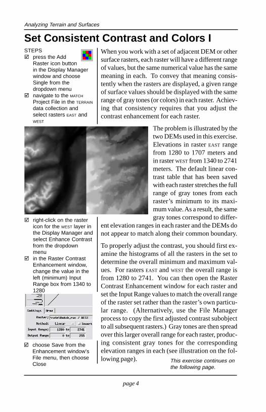
When you work with a set of adjacent DEM or othersurface rasters, each raster will have a different rangeof values, but the same numerical value has the samemeaning in each. To convey that meaning consis-tently when the rasters are displayed, a given rangeof surface values should be displayed with the samerange of gray tones (or colors) in each raster. Achiev-ing that consistency requires that you adjust thecontrast enhancement for each raster.

The problem is illustrated by thetwo DEMs used in this exercise.Elevations in raster EAST rangefrom 1280 to 1707 meters andin raster WEST from 1340 to 2741meters. The default linear con-trast table that has been savedwith each raster stretches the fullrange of gray tones from eachraster’s minimum to its maxi-mum value. As a result, the samegray tones correspond to differ-

ent elevation ranges in each raster and the DEMs donot appear to match along their common boundary.

To properly adjust the contrast, you should first ex-amine the histograms of all the rasters in the set todetermine the overall minimum and maximum val-ues. For rasters EAST and WEST the overall range isfrom 1280 to 2741. You can then open the RasterContrast Enhancement window for each raster andset the Input Range values to match the overall rangeof the raster set rather than the raster’s own particu-lar range. (Alternatively, use the File Managerprocess to copy the first adjusted contrast subobjectto all subsequent rasters.) Gray tones are then spreadover this larger overall range for each raster, produc-ing consistent gray tones for the correspondingelevation ranges in each (see illustration on the fol-lowing page).

choose Save from theEnhancement window’sFile menu, then chooseClose

This exercise continues onthe following page.

Set Consistent Contrast and Colors I


page 5

STEPSrepeat the last threesteps for the EAST layer,but change the right(maximum) Input Rangevalue from 1707 to 2741redraw the Viewwindow

right-click on the rastericon for the WEST layerand select Edit Colorsfrom the dropdownmenuclick on the Palettemenu in the ColorPalette Editor windowand select the EarthTones paletteif the Earth Tones paletteis not shown on theinitial menu, chooseMore Palettes and selectit from the scrolling list inthe Standard ColorPalettes window andclick [OK]choose Save As fromthe Color PaletteEditor’s File menu andsave the palette as asubobject of raster WEST

repeat the last step andsave the palette as asubobject of raster EAST

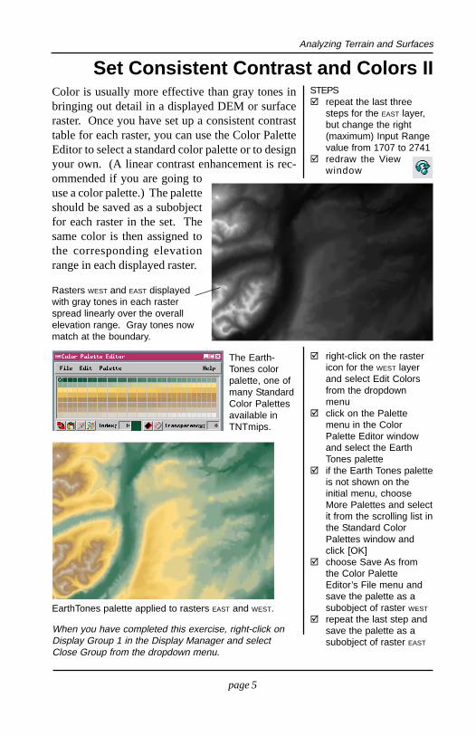
Rasters WEST and EAST displayedwith gray tones in each rasterspread linearly over the overallelevation range. Gray tones nowmatch at the boundary.

Set Consistent Contrast and Colors IIColor is usually more effective than gray tones inbringing out detail in a displayed DEM or surfaceraster. Once you have set up a consistent contrasttable for each raster, you can use the Color PaletteEditor to select a standard color palette or to designyour own. (A linear contrast enhancement is rec-ommended if you are going touse a color palette.) The paletteshould be saved as a subobjectfor each raster in the set. Thesame color is then assigned tothe corresponding elevationrange in each displayed raster.

EarthTones palette applied to rasters EAST and WEST.

The Earth-Tones colorpalette, one ofmany StandardColor Palettesavailable inTNTmips.

When you have completed this exercise, right-click onDisplay Group 1 in the Display Manager and selectClose Group from the dropdown menu.


page 6

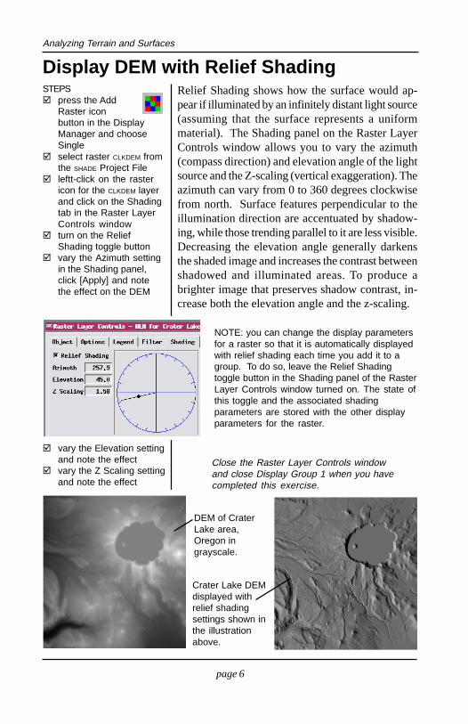
Display DEM with Relief ShadingSTEPS

press the AddRaster iconbutton in the DisplayManager and chooseSingleselect raster CLKDEM fromthe SHADE Project Fileleftt-click on the rastericon for the CLKDEM layerand click on the Shadingtab in the Raster LayerControls windowturn on the ReliefShading toggle buttonvary the Azimuth settingin the Shading panel,click [Apply] and notethe effect on the DEM

vary the Elevation settingand note the effectvary the Z Scaling settingand note the effect

DEM of CraterLake area,Oregon ingrayscale.

Crater Lake DEMdisplayed withrelief shadingsettings shown inthe illustrationabove.

Close the Raster Layer Controls windowand close Display Group 1 when you havecompleted this exercise.

Relief Shading shows how the surface would ap-pear if illuminated by an infinitely distant light source(assuming that the surface represents a uniformmaterial). The Shading panel on the Raster LayerControls window allows you to vary the azimuth(compass direction) and elevation angle of the lightsource and the Z-scaling (vertical exaggeration). Theazimuth can vary from 0 to 360 degrees clockwisefrom north. Surface features perpendicular to theillumination direction are accentuated by shadow-ing, while those trending parallel to it are less visible.Decreasing the elevation angle generally darkensthe shaded image and increases the contrast betweenshadowed and illuminated areas. To produce abrighter image that preserves shadow contrast, in-crease both the elevation angle and the z-scaling.

NOTE: you can change the display parametersfor a raster so that it is automatically displayedwith relief shading each time you add it to agroup. To do so, leave the Relief Shadingtoggle button in the Shading panel of the RasterLayer Controls window turned on. The state ofthis toggle and the associated shadingparameters are stored with the other displayparameters for the raster.


page 7

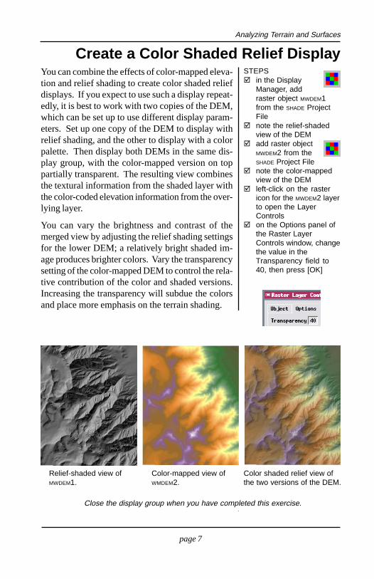
Create a Color Shaded Relief DisplaySTEPS

in the DisplayManager, addraster object MWDEM1from the SHADE ProjectFilenote the relief-shadedview of the DEMadd raster objectMWDEM2 from theSHADE Project Filenote the color-mappedview of the DEMleft-click on the rastericon for the MWDEM2 layerto open the LayerControlson the Options panel ofthe Raster LayerControls window, changethe value in theTransparency field to40, then press [OK]

You can combine the effects of color-mapped eleva-tion and relief shading to create color shaded reliefdisplays. If you expect to use such a display repeat-edly, it is best to work with two copies of the DEM,which can be set up to use different display param-eters. Set up one copy of the DEM to display withrelief shading, and the other to display with a colorpalette. Then display both DEMs in the same dis-play group, with the color-mapped version on toppartially transparent. The resulting view combinesthe textural information from the shaded layer withthe color-coded elevation information from the over-lying layer.

You can vary the brightness and contrast of themerged view by adjusting the relief shading settingsfor the lower DEM; a relatively bright shaded im-age produces brighter colors. Vary the transparencysetting of the color-mapped DEM to control the rela-tive contribution of the color and shaded versions.Increasing the transparency will subdue the colorsand place more emphasis on the terrain shading.

Relief-shaded view ofMWDEM1.

Color-mapped view ofWMDEM2.

Color shaded relief view ofthe two versions of the DEM.

Close the display group when you have completed this exercise.


page 8

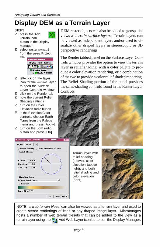
Display DEM as a Terrain LayerSTEPS

press the AddTerrain iconbutton in the DisplayManagerselect raster MWDEM1from the SHADE ProjectFile

Terrain layer withrelief-shading(above), colorelevation (aboveright), and bothrelief shading andcolor elevation(right).

DEM raster objects can also be added to geospatialviews as terrain surface layers. Terrain layers canbe viewed as independent layers and/or used to vi-sualize other draped layers in stereoscopic or 3Dperspective renderings.

The Render tabbed panel on the Surface Layer Con-trols window provides the option to view the terrainlayer in relief shading, with a color palette to pro-duce a color elevation rendering, or a combinationof the two to provide a color relief shaded rendering.The Relief Shading portion of the panel providesthe same shading controls found in the Raster LayerControls.

NOTE: a web terrain tileset can also be viewed as a terrain layer and used tocreate stereo renderings of itself or any draped image layer. MicroImageshosts a number of web terrain tilesets that can be added to the view as aterrain layer using the Add Web Layer icon button on the Display Manager.

left-click on the layericon for the MWDEM1 layerto open the SurfaceLayer Controls windowclick on the Render tabnote the current ReliefShading settingsturn on the ColorElevation radio buttonin the Elevation Colorcontrols, choose EarthTones from the Palettemenu and press [Apply]turn on the Both radiobutton and press [OK]


page 9

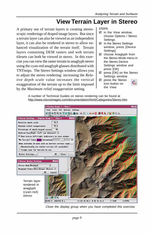
View Terrain Layer in StereoSTEPS

in the View window,choose Options / StereoSettingsIn the Stereo Settingswindow, press [DeviceSettings]choose Anaglyph fromthe Stereo Mode menu inthe Stereo DeviceSettings window andpress [OK]press [OK] on the StereoSettings windowpress the Stereoicon button onthe View


A number of Technical Guides on stereo rendering can be found athttp://www.microimages.com/documentation/html/Categories/Stereo.htm

Terrain layerrendered inanaglyph(cyan-red)stereo

A primary use of terrain layers is creating stereo-scopic renderings of draped image layers. But sincea terrain layer can also be viewed as an independentlayer, it can also be rendered in stereo to allow en-hanced visualization of the terrain itself. Terrainlayers containing DEM rasters and web terraintilesets can both be viewed in stereo. In this exer-cise you can view the raster terrain in anaglyph stereousing the cyan-red anaglyph glasses distributed withTNTmips. The Stereo Settings window allows youto adjust the stereo rendering: increasing the Rela-tive depth scale value increases the verticalexaggeration of the terrain up to the limit imposedby the Maximum relief exaggeration setting.


page 10

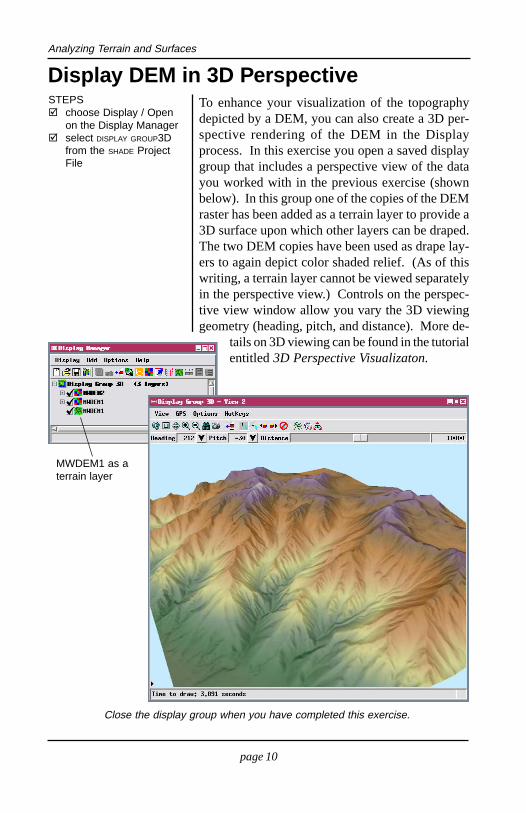
Display DEM in 3D PerspectiveSTEPS

choose Display / Openon the Display Managerselect DISPLAY GROUP3Dfrom the SHADE ProjectFile


To enhance your visualization of the topographydepicted by a DEM, you can also create a 3D per-spective rendering of the DEM in the Displayprocess. In this exercise you open a saved displaygroup that includes a perspective view of the datayou worked with in the previous exercise (shownbelow). In this group one of the copies of the DEMraster has been added as a terrain layer to provide a3D surface upon which other layers can be draped.The two DEM copies have been used as drape lay-ers to again depict color shaded relief. (As of thiswriting, a terrain layer cannot be viewed separatelyin the perspective view.) Controls on the perspec-tive view window allow you vary the 3D viewinggeometry (heading, pitch, and distance). More de-

tails on 3D viewing can be found in the tutorialentitled 3D Perspective Visualizaton.

MWDEM1 as aterrain layer


page 11

STEPSchoose Terrain /Topographic Propertiesfrom the TNTmips menuclick [Raster...]navigate to the SLOPE

Project File and selectobject DEM_S1from the Surface-Fittingmenu choose Exact fitto 4 nearest neighborsand center cell

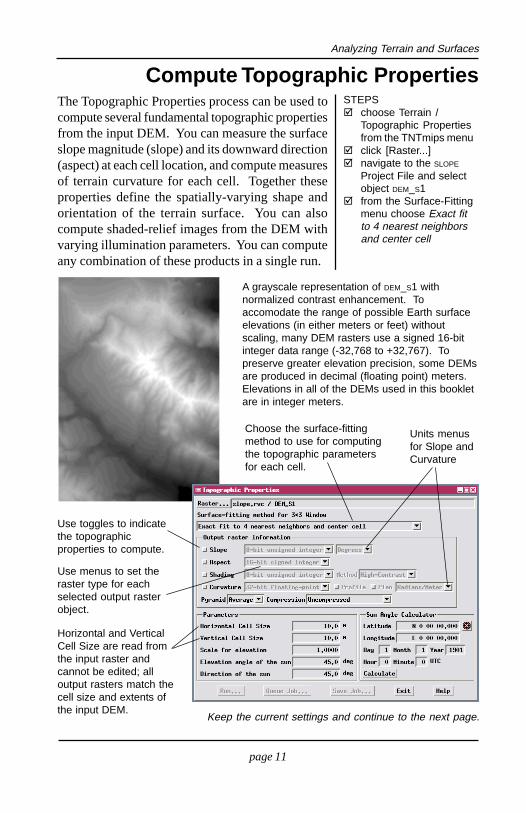
Compute Topographic PropertiesThe Topographic Properties process can be used tocompute several fundamental topographic propertiesfrom the input DEM. You can measure the surfaceslope magnitude (slope) and its downward direction(aspect) at each cell location, and compute measuresof terrain curvature for each cell. Together theseproperties define the spatially-varying shape andorientation of the terrain surface. You can alsocompute shaded-relief images from the DEM withvarying illumination parameters. You can computeany combination of these products in a single run.

A grayscale representation of DEM_S1 withnormalized contrast enhancement. Toaccomodate the range of possible Earth surfaceelevations (in either meters or feet) withoutscaling, many DEM rasters use a signed 16-bitinteger data range (-32,768 to +32,767). Topreserve greater elevation precision, some DEMsare produced in decimal (floating point) meters.Elevations in all of the DEMs used in this bookletare in integer meters.

Choose the surface-fittingmethod to use for computingthe topographic parametersfor each cell.

Use toggles to indicatethe topographicproperties to compute.

Use menus to set theraster type for eachselected output rasterobject.

Horizontal and VerticalCell Size are read fromthe input raster andcannot be edited; alloutput rasters match thecell size and extents ofthe input DEM.

Keep the current settings and continue to the next page.

Units menusfor Slope andCurvature


page 12

Compute Slope and Aspect

press [Run...]use the standard SelectObjects dialog windowto name a new ProjectFile and accept thedefault names for theoutput Slope and Aspectraster objectsuse the Display processto view theoutput Slopeand Aspectrasterobjectsclose theDisplaygroup whenyou havecompletedthe exercise

STEPSturn on the Slope andAspect toggle buttonsand make sure that theShading and Curvaturetoggles are off.choose Degrees fromthe units menu for Slopechoose 32-bit floatingpoint from the rasterdata type menu for theSlope raster, and 16-bitsigned integer for theAspect raster

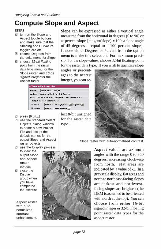
Slope raster with auto-normalized contrast.

Slope can be expressed as either a vertical anglemeasured from the horizontal in degrees (0 to 90) oras percent slope [tangent(slope) x 100; a slope angleof 45 degrees is equal to a 100 percent slope].Choose either Degrees or Percent from the optionmenu to make this selection. For maximum preci-sion for the slope values, choose 32-bit floating-pointfor the raster data type. If you wish to quantize slopeangles or percent-ages to the nearestinteger, you can se-

lect 8-bit unsignedfor the raster datatype.

Aspect values are azimuthangles with the range 0 to 360degrees, increasing clockwisefrom north. Flat areas areindicated by a value of -1. In agrayscale display, flat areas andnorth to northeast-facing slopesare darkest and northwest-facing slopes are brightest (theDEM is assumed to be orientedwith north at the top). You canchoose from either 16-bitsigned integer or 32-bit floatingpoint raster data types for theaspect raster.

Aspect rasterwith auto-normalizedcontrastenhancement.


page 13

STEPSturn off the Slope andAspect toggle buttonsturn on the Curvaturetoggle and make surethat the Profile and Plantoggles are both turnedonchoose 32-bit floatingpoint from the rasterdata type menu forCurvaturechoose Radians/Meterfrom the units menu forCurvaturepress [Run...]accept the defaultnames for the outputcurvature raster objectsuse the Display processto view the output rasterobjects

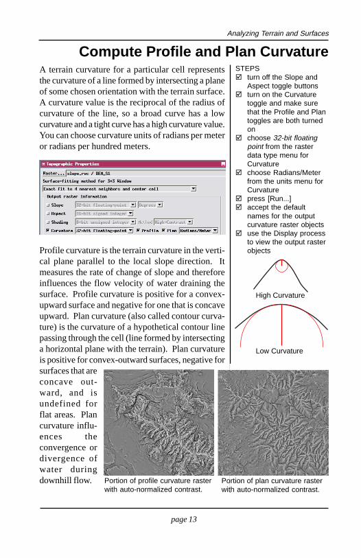
High Curvature

A terrain curvature for a particular cell representsthe curvature of a line formed by intersecting a planeof some chosen orientation with the terrain surface.A curvature value is the reciprocal of the radius ofcurvature of the line, so a broad curve has a lowcurvature and a tight curve has a high curvature value.You can choose curvature units of radians per meteror radians per hundred meters.

Low Curvature

Portion of profile curvature rasterwith auto-normalized contrast.

Profile curvature is the terrain curvature in the verti-cal plane parallel to the local slope direction. Itmeasures the rate of change of slope and thereforeinfluences the flow velocity of water draining thesurface. Profile curvature is positive for a convex-upward surface and negative for one that is concaveupward. Plan curvature (also called contour curva-ture) is the curvature of a hypothetical contour linepassing through the cell (line formed by intersectinga horizontal plane with the terrain). Plan curvatureis positive for convex-outward surfaces, negative forsurfaces that areconcave out-ward, and isundefined forflat areas. Plancurvature influ-ences theconvergence ordivergence ofwater duringdownhill flow. Portion of plan curvature raster

with auto-normalized contrast.

Compute Profile and Plan Curvature


page 14

Compute ShadingSTEPS

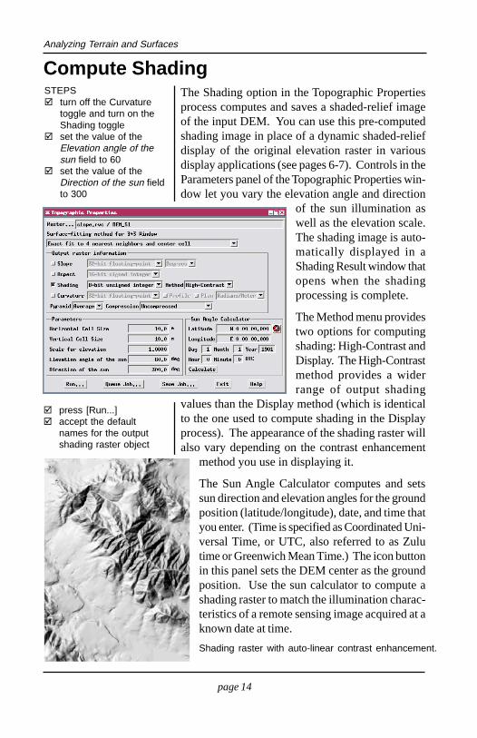
turn off the Curvaturetoggle and turn on theShading toggleset the value of theElevation angle of thesun field to 60set the value of theDirection of the sun fieldto 300

press [Run...]accept the defaultnames for the outputshading raster object

The Shading option in the Topographic Propertiesprocess computes and saves a shaded-relief imageof the input DEM. You can use this pre-computedshading image in place of a dynamic shaded-reliefdisplay of the original elevation raster in variousdisplay applications (see pages 6-7). Controls in theParameters panel of the Topographic Properties win-dow let you vary the elevation angle and direction

of the sun illumination aswell as the elevation scale.The shading image is auto-matically displayed in aShading Result window thatopens when the shadingprocessing is complete.

The Method menu providestwo options for computingshading: High-Contrast andDisplay. The High-Contrastmethod provides a widerrange of output shading

values than the Display method (which is identicalto the one used to compute shading in the Displayprocess). The appearance of the shading raster willalso vary depending on the contrast enhancement

method you use in displaying it.

The Sun Angle Calculator computes and setssun direction and elevation angles for the groundposition (latitude/longitude), date, and time thatyou enter. (Time is specified as Coordinated Uni-versal Time, or UTC, also referred to as Zulutime or Greenwich Mean Time.) The icon buttonin this panel sets the DEM center as the groundposition. Use the sun calculator to compute ashading raster to match the illumination charac-teristics of a remote sensing image acquired at aknown date at time.

Shading raster with auto-linear contrast enhancement.


page 15

Surface-Fitting MethodsSTEPS

open the Surface-fittingmethod menu on theTopographic Propertieswindow

Topographic properties are computed for each cellby using a moving 3 by 3 kernel of cells to computefirst and second derivatives of the local surface inthe line and column directions. The choice of cellswithin this kernel and the weighting factors appliedcan be varied to represent different mathematical ap-proximations of the local surface. The fivesurface-fitting methods shown in the sidebar areavailable.

The first listed method uses a cross-shaped kerneland fits the surface exactly to all five cell values;this method produces topographic parameters thatare most faithful to the raw elevation values. How-ever, most DEMs contain elevation errors to varyingdegrees. To mitigate the effects of such elevation“noise”, the other four surface-fitting methods useelevations from all nine kernel cells to com-pute a curved surface that is a “best fit”approximation of the kernel values. As a re-sult, these quadratic methods all introduce adegree of averaging and smoothing to the to-pographic parameters. The quadraticmethods differ from each other in how the val-ues of the more distant corner cells in thekernel are weighted relative to the middle cellsalong the kernel edges. In addition, only thelast quadratic method in the list forces thequadratic surface to exactly match the eleva-tion of the central cell in the kernel. Differencesbetween the topographic parameters createdusing the four quadratic surface-fitting meth-ods are slight, but may be locally significant.

Exact fit to 4 nearestneighbors and center cell

Quadratic surface, least-squares fit

Quadratic surface, least-squares fit, weighted by1/distance2

Quadratic surface, least-squares fit, weighted by1/distance

Quadratic surface, leastsquares fit, match centralcell

Surface-fitting methods

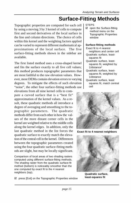
Exact fit to 4 nearest neighbors

Quadratic surface,least-squares fit

Comparison of local areas of two shading rasterscomputed using different surface-fitting methods.The shading raster from the quadratic surface-fitmethod (bottom) is noticeably smoother than theone computed by exact fit to the 4 nearestneighbors (top).

press [Exit] on the Topographic Properties window


page 16

Viewshed AnalysisSTEPS

choose Terrain /Viewshed from theTNTmips menuin the Select Objectwindow, navigate to theVIEWSHED Project File andselect object DEM_V1move the mouse overthe center of the circlegraphic in the View; thecursor should assume across-hairs shapedrag the center of thecircle graphic to thelocation shown in theillustrationwith the cursor over theView, use the arrow keyson your keyboard tomove the viewpoint until

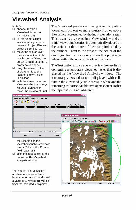
The Viewshed process allows you to compute aviewshed from one or more positions on or abovethe surface represented by the input elevation raster.This raster is displayed in a View window and aninitial viewpoint location is automatically placed onthe surface at the center of the raster, indicated bythe number 1 next to the cross at the center of thecircle graphic. You can reposition this point any-where within the area of the elevation raster.

The Test option allows you to preview the results bycomputing a temporary viewshed raster that is dis-played in the Viewshed Analysis window. Thetemporary viewshed raster is displayed with cellswithin the viewshed (visible areas) in white and theremaining cells (non-visible areas) transparent so thatthe input raster is not obscured.

the Line field in theViewshed Analysis windowreads 391 and the Columnfield reads 158click the Test button at thebottom of the ViewshedAnalysis window

The results of a Viewshedanalysis are encoded as abinary raster in which cells witha value of 1 (white) are visiblefrom the selected viewpoints.


page 17

Adjust Viewpoint HeightSTEPS

type 30 in the Heighttext box in the ViewshedAnalysis window andpress [Enter] or [Tab]press [Test]

To identify cells that are visible from your selectedviewpoints, the viewshed process analyzes the 3Dlines connecting each viewpoint and each cell. If asightline remains entirely above the ground surfacebetween the viewpoint and cell, the cell is visiblefrom that viewpoint.

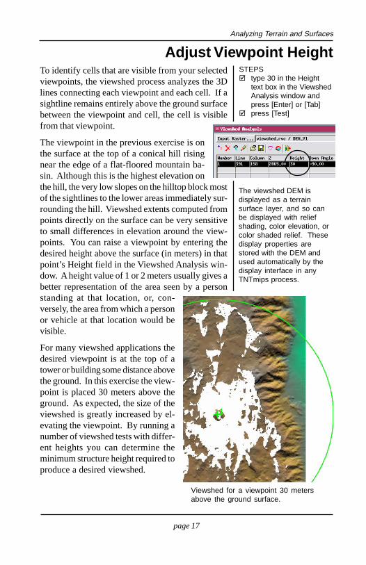
The viewpoint in the previous exercise is onthe surface at the top of a conical hill risingnear the edge of a flat-floored mountain ba-sin. Although this is the highest elevation onthe hill, the very low slopes on the hilltop block mostof the sightlines to the lower areas immediately sur-rounding the hill. Viewshed extents computed frompoints directly on the surface can be very sensitiveto small differences in elevation around the view-points. You can raise a viewpoint by entering thedesired height above the surface (in meters) in thatpoint’s Height field in the Viewshed Analysis win-dow. A height value of 1 or 2 meters usually gives abetter representation of the area seen by a personstanding at that location, or, con-versely, the area from which a personor vehicle at that location would bevisible.

For many viewshed applications thedesired viewpoint is at the top of atower or building some distance abovethe ground. In this exercise the view-point is placed 30 meters above theground. As expected, the size of theviewshed is greatly increased by el-evating the viewpoint. By running anumber of viewshed tests with differ-ent heights you can determine theminimum structure height required toproduce a desired viewshed.

Viewshed for a viewpoint 30 metersabove the ground surface.

The viewshed DEM isdisplayed as a terrainsurface layer, and so canbe displayed with reliefshading, color elevation, orcolor shaded relief. Thesedisplay properties arestored with the DEM andused automatically by thedisplay interface in anyTNTmips process.


page 18

Adjust Range and Field of ViewSTEPS

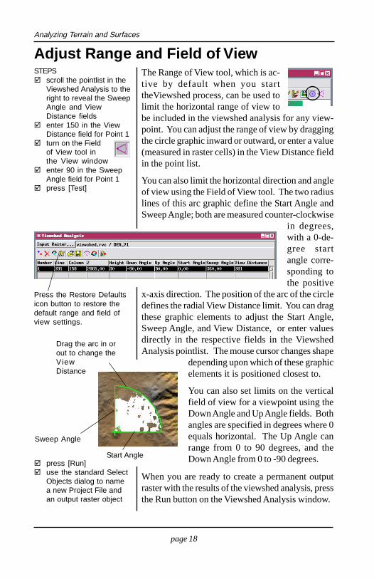
scroll the pointlist in theViewshed Analysis to theright to reveal the SweepAngle and ViewDistance fieldsenter 150 in the ViewDistance field for Point 1turn on the Fieldof View tool inthe View windowenter 90 in the SweepAngle field for Point 1press [Test]

The Range of View tool, which is ac-tive by default when you starttheViewshed process, can be used tolimit the horizontal range of view tobe included in the viewshed analysis for any view-point. You can adjust the range of view by draggingthe circle graphic inward or outward, or enter a value(measured in raster cells) in the View Distance fieldin the point list.

You can also limit the horizontal direction and angleof view using the Field of View tool. The two radiuslines of this arc graphic define the Start Angle andSweep Angle; both are measured counter-clockwise

in degrees,with a 0-de-gree startangle corre-sponding tothe positive

x-axis direction. The position of the arc of the circledefines the radial View Distance limit. You can dragthese graphic elements to adjust the Start Angle,Sweep Angle, and View Distance, or enter valuesdirectly in the respective fields in the ViewshedAnalysis pointlist. The mouse cursor changes shape

depending upon which of these graphicelements it is positioned closest to.

You can also set limits on the verticalfield of view for a viewpoint using theDown Angle and Up Angle fields. Bothangles are specified in degrees where 0equals horizontal. The Up Angle canrange from 0 to 90 degrees, and theDown Angle from 0 to -90 degrees.press [Run]

use the standard SelectObjects dialog to namea new Project File andan output raster object

When you are ready to create a permanent outputraster with the results of the viewshed analysis, pressthe Run button on the Viewshed Analysis window.

Press the Restore Defaultsicon button to restore thedefault range and field ofview settings.

Drag the arc in orout to change theViewDistance

Start Angle

Sweep Angle


page 19

Viewshed from Multiple ViewpointsSTEPS

reset the Sweep Anglefor Point 1 to 360press the Addicon button on theViewshedAnalysis windowdrag the new Point 2 toa location in the northernhalf of the rasterset the Height of Point 2to 30set the View Distancefor Point 2 to 150press [Test]

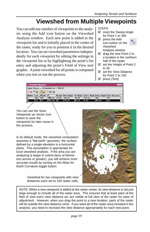
You can add any number of viewpoints to the analy-sis using the Add icon button on the ViewshedAnalysis window. Each new point is added to theviewpoint list and is initially placed in the center ofthe raster, ready for you to position it in the desiredlocation. You can set viewshed parameters indepen-dently for each viewpoint by editing the settings inthe viewpoint list or by highlighting the point’s listentry and adjusting the point’s Field of View toolgraphic. A joint viewshed for all points is computedwhen you test or run the process.

Viewshed for two viewpoints with viewdistances each set to 150 raster cells.

NOTE: When a new viewpoint is added at the raster center, its view distance is set justlarge enough to include all of the raster area. This ensures that at least parts of thefield of view tool’s view distance arc are visible at full view of the raster for ease ofadjustment. However, when you drag the point to a new location, parts of the rasterwill lie outside the view distance circle. If you want all of the raster area included in theanalysis, you need to increase the view distance appropriately for each new point.

In its default mode, the viewshed computationassumes a “flat-earth” geometry: the surfacedefined by a single elevation is a horizontalplane. This assumption is appropriate forlocal viewshed analysis. If the area you areanalyzing is larger in extent (tens of kilome-ters across or greater), you will achieve moreaccurate results by turning on the Allow forEarth Curvature toggle button.

You can use the SaveViewpoints as Vector iconbutton to save theviewpoints for later reuse inthe process.


page 20

Load Saved ViewpointsSTEPS

press the LoadViewpoints iconbutton on theViewshed Analysiswindow and chooseLoad from the dropdownmenuselect vector object VPTS

from the VIEWSHED

Project Fileenter 2.0 in the Heightfield for each of the 9viewpointsenter 25 in thePercentage ofViewpoints field at thebottom of the ViewshedAnalysis window

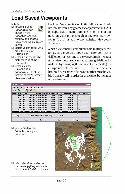
The Load Viewpoints icon button allows you to addviewpoints from any geometric object (vector, CAD,or shape) that contains point elements. The buttonmenu provides options to clear any existing view-points (Load) or add to any existing viewpoints(Append).

When a viewshed is computed from multiple view-points, in the default mode any raster cell that isvisible from at least one of the viewpoints is includedin the viewshed. You can set stricter guidelines forvisibility by changing the value in the Percentage ofViewpoints field (default = 0). This field sets thethreshold percentage of viewpoints that must be vis-ible from any cell in order for that cell to be includedin the viewshed.

close the Viewshed processby pressing [Exit] when youhave completed this exercise

press [Test] on theViewshed Analysiswindow


page 21

STEPSselect Terrain / Cut andFill Analysis from theTNTmips menupress the SelectDEMs icon buttonon the Cut / Fill windowin the Select DEMswindow, first selectraster FILLED from thePONDS Project File as theNew rasterthen select raster PONDS

from the same file asthe Old rasterpress [Run] and createan output Project Fileuse the Auto-Namebutton to accept thedefault names for theBoundaries vector andDifference raster

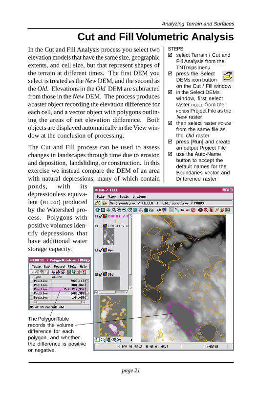
Cut and Fill Volumetric AnalysisIn the Cut and Fill Analysis process you select twoelevation models that have the same size, geographicextents, and cell size, but that represent shapes ofthe terrain at different times. The first DEM youselect is treated as the New DEM, and the second asthe Old. Elevations in the Old DEM are subtractedfrom those in the New DEM. The process producesa raster object recording the elevation difference foreach cell, and a vector object with polygons outlin-ing the areas of net elevation difference. Bothobjects are displayed automatically in the View win-dow at the conclusion of processing.

The Cut and Fill process can be used to assesschanges in landscapes through time due to erosionand deposition, landsliding, or construction. In thisexercise we instead compare the DEM of an areawith natural depressions, many of which containponds, with itsdepressionless equiva-lent (FILLED) producedby the Watershed pro-cess. Polygons withpositive volumes iden-tify depressions thathave additional waterstorage capacity.

The PolygonTablerecords the volumedifference for eachpolygon, and whetherthe difference is positiveor negative.


page 22

Advanced Software for Geospatial Analysis

MicroImages, Inc.

MicroImages, Inc. publishes a complete line of professional software for advanced geospatialdata visualization, analysis, and publishing. Contact us or visit our web site for detailed prod-uct information.

TNTmips Pro TNTmips Pro is a professional system for fully integrated GIS, imageanalysis, CAD, TIN, desktop cartography, and geospatial database management.

TNTmips Basic TNTmips Basic is a low-cost version of TNTmips for small projects.

TNTmips Free TNTmips Free is a free version of TNTmips for students and profession-als with small projects. You can download TNTmips Free from MicroImages’ web site.

TNTedit TNTedit provides interactive tools to create, georeference, and edit vector, image,CAD, TIN, and relational database project materials in a wide variety of formats.

TNTview TNTview has the same powerful display features as TNTmips and is perfect forthose who do not need the technical processing and preparation features of TNTmips.

TNTatlas TNTatlas lets you publish and distribute your spatial project materials on CD orDVD at low cost. TNTatlas CDs/DVDs can be used on any popular computing platform.

Indexaspect........................................3,11,12color palette.....................................5,7color shaded relief............................7,8,10contrast enhancement.......................4,5cut and fill..........................................3,21h i s togram. . . . . . . . . . . . . . . . . . . . . . . . . . . . . . . . . 4relief shading...........................6,7,8,10,17shading raster.................................3,14,15slope....... . . . . . . . . . . . . . . . . . . . . . . . . . . . . .3,11,12

stereo................................................9transparency..................................7,17v i e w p o i n t . . . . . . . . . . . . . . . . . . . . . . . 1 6 - 2 0

field of view..........................18he igh t . . . . . . . . . . . . . . . . . . . . . . . . . . . . . . . . 17

viewshed. . . . . . . . . . . . . . . . . . . . . . . . . . . .3 ,16-20viewshed test...................................16w a t e r s h e d . . . . . . . . . . . . . . . . . . . . . . . . . . . 3 , 1 9

TERRAIN

ANALYSIS

Documents

Analyzing Terrain and Surfaces - MicroImages, Inc