Analyzing the effects of geological and parameter uncertainty on prediction of groundwater head

Hydrol. Earth Syst. Sci., 17, 3245–3260, 2013www.hydrol-earth-syst-sci.net/17/3245/2013/doi:10.5194/hess-17-3245-2013© Author(s) 2013. CC Attribution 3.0 License.

EGU Journal Logos (RGB)

Advances in Geosciences

Open A

ccess

Natural Hazards and Earth System

Sciences

Open A

ccess

Annales Geophysicae

Open A

ccess

Nonlinear Processes in Geophysics

Open A

ccess

Atmospheric Chemistry

and Physics

Open A

ccess

Atmospheric Chemistry

and Physics

Open A

ccess

Discussions

Atmospheric Measurement

Techniques

Open A

ccess

Atmospheric Measurement

Techniques

Open A

ccess

Discussions

Biogeosciences

Open A

ccess

Open A

ccess

BiogeosciencesDiscussions

Climate of the Past

Open A

ccess

Open A

ccess

Climate of the Past

Discussions

Earth System Dynamics

Open A

ccess

Open A

ccess

Earth System Dynamics

Discussions

GeoscientificInstrumentation

Methods andData Systems

Open A

ccess

GeoscientificInstrumentation

Methods andData Systems

Open A

ccess

Discussions

GeoscientificModel Development

Open A

ccess

Open A

ccess

GeoscientificModel Development

Discussions

Hydrology and Earth System

SciencesO

pen Access

Hydrology and Earth System

Sciences

Open A

ccess

Discussions

Ocean Science

Open A

ccess

Open A

ccess

Ocean ScienceDiscussions

Solid Earth

Open A

ccess

Open A

ccess

Solid EarthDiscussions

The Cryosphere

Open A

ccess

Open A

ccess

The CryosphereDiscussions

Natural Hazards and Earth System

Sciences

Open A

ccess

Discussions

Analyzing the effects of geological and parameter uncertainty onprediction of groundwater head and travel time

X. He1, T. O. Sonnenborg2, F. Jørgensen2, A.-S. Høyer2,3, R. R. Møller2, and K. H. Jensen1

1Department of Geosciences and Natural Resource Management, Copenhagen University, Copenhagen, Denmark2Geological Survey of Denmark and Greenland (GEUS), Copenhagen, Denmark3Department of Earth Sciences, Aarhus University, Aarhus, Denmark

Correspondence to:X. He ([email protected])

Received: 14 February 2013 – Published in Hydrol. Earth Syst. Sci. Discuss.: 6 March 2013Revised: 11 June 2013 – Accepted: 8 July 2013 – Published: 16 August 2013

Abstract. Uncertainty of groundwater model predictions hasin the past mostly been related to uncertainty in the hydraulicparameters, whereas uncertainty in the geological structurehas not been considered to the same extent. Recent devel-opments in theoretical methods for quantifying geologicaluncertainty have made it possible to consider this factor ingroundwater modeling. In this study we have applied themultiple-point geostatistical method (MPS) integrated in theStanford Geostatistical Modeling Software (SGeMS) for ex-ploring the impact of geological uncertainty on groundwa-ter flow patterns for a site in Denmark. Realizations fromthe geostatistical model were used as input to a groundwa-ter model developed from Modular three-dimensional finite-difference ground-water model (MODFLOW) within theGroundwater Modeling System (GMS) modeling environ-ment. The uncertainty analysis was carried out in three sce-narios involving simulation of groundwater head distributionand travel time. The first scenario implied 100 stochastic ge-ological models all assigning the same hydraulic parametersfor the same geological units. In the second scenario the same100 geological models were subjected to model optimiza-tion, where the hydraulic parameters for each of them wereestimated by calibration against observations of hydraulichead and stream discharge. In the third scenario each geolog-ical model was run with 216 randomized sets of parameters.The analysis documented that the uncertainty on the concep-tual geological model was as significant as the uncertaintyrelated to the embedded hydraulic parameters.

1 Introduction

With the prevalent application of groundwater modeling, theinherent uncertainties associated with model simulation arewell acknowledged (Delhomme, 1979; Beven and Binley,1992; Feyen et al., 2001; Hassan et al., 2008). Dettinger andWilson (1981) divided uncertainty in groundwater systemsinto two classes: intrinsic uncertainty and information uncer-tainty. A subsurface property, such as hydraulic conductiv-ity, is considered as intrinsic uncertainty due to its spatialstochastic variations. The spatial variation is affected by dif-ferences in large-scale parameter values between geologicalunits superimposed by smaller-scale variation within the in-dividual units. Webb and Anderson (1996), Journel and Al-abert (1990), Carle et al. (1998) and Mariethoz et al. (2009)have suggested to incorporate these two contributions in amodeling framework by first defining the overall geologi-cal structure and then incorporating the smaller-scale spa-tial heterogeneity of the hydrogeological parameters withinthe units.

A common approach to simulate spatial heterogeneityin hydrogeology is to use geostatistics, and the traditionalmethod is to employ variogram-based techniques (Del-homme, 1979; Wingle and Poeter, 1993; Johnson, 1995;Klise et al., 2009). Despite that these traditional methodshave been applied extensively during the last three decades,they only consider correlation between two spatial locations,which often fails to depict distinct largely connected geolog-ical structures. Further, due to mathematical simplificationsthese methods can only capture a limited number of datatypes (Caers and Zhang, 2004; Journel, 2005). Renard (2007)

Published by Copernicus Publications on behalf of the European Geosciences Union.

3246 X. He et al.: Prediction of groundwater head and travel time

proposed three alternative techniques: the truncated pluri-Gaussian method, the continuous-lag Markov chain, andthe multiple-point geostatistical approach (MPS), where thelatter was viewed as the most appealing method. The ad-vantages of MPS have been demonstrated by, e.g., Stre-belle (2002), Caers and Zhang (2004), Liu et al. (2005), Jour-nel and Zhang (2006), Liu (2006), and Strebelle (2006). Eventhough the ability of using MPS for 3-D simulations was ac-knowledged, only 2-D simulations were presented in thesestudies. Fundamental to the application of MPS is the defini-tion of an appropriate training image (TI), which is a 2-D or3-D image of the geological characteristics or patterns of themodel area (Caers and Zhang, 2004). In the study of LakeChad Basin, Le Coz et al. (2011) made a 3-D TI by replicat-ing a single horizontal 2-D TI. However, they also realizedthat in this way the degree of similarity between two succes-sive layers is maximized vertically, resulting in a very highnugget effect from 3-D simulations. Comunian et al. (2011)demonstrated a hierarchical multiple-point method with acomplicated framework, which includes breaking large-scalestructures into a number of subregions and application of3-D MPS to each heterogeneous subregion. Overall, theirthree-dimensional TI was generated by object-based tech-niques for which the parameters were estimated manually bytrial and error from 2-D observed sections. Honarkhah andCaers (2012) demonstrated a new MPS modeling paradigmwith 3-D TI, but the data source and method of generatingthe 3-D TI was not mentioned. Multiple-point geostatistics isindeed appealing in stochastic hydrogeology, but so far theapplication to 3-D problems seems to be constrained by thedifficulty of acquiring a full 3-D TI.

Parameter uncertainty is usually analyzed by applyingMonte Carlo-based stochastic approaches, and the Gener-alized Likelihood Uncertainty Estimation (GLUE) (Bevenand Binley, 1992) is one of the most popular methodolo-gies due to its conceptual simplicity and ease of implemen-tation. However, the method has been subject to criticismas the likelihood measure is “less formal” (Mantovan andTodini, 2006; Mantovan et al., 2007), the choice of like-lihood measure is subjective and the updating process re-quires abundant observations (Feyen et al., 2001). Recently,several formal Bayesian methods for highly parameterizedgroundwater models have emerged (Hendricks Franssen etal., 2004; Tonkin and Doherty, 2005; Vrugt et al., 2008).These global search methods have the advantage of providinga more robust uncertainty analysis but they are also highly-CPU demanding and time-consuming.

Several studies have been reported in the literature on theimpact of parameter and geological uncertainty on ground-water modeling. Freeze et al. (1990) were among the first tojointly consider both geological and parameter uncertainty.Abbaspou et al. (1998) proposed the uncertainty analysisframework BUDA (Bayesian Uncertainty Development Al-gorithm). Despite its ability to quantify uncertainty by con-ditioning on both hard and soft data, the approach for analyz-

ing uncertainty is based on two-point-based kriging. Feyenet al. (2001) presented a study on stochastic capture zonedelineation by using the GLUE method. The stochastic hy-draulic conductivity distribution was generated by sequen-tial Gaussian simulation, but the distribution was still gov-erned by a two-point covariance-based function. Harrar etal. (2003) also conducted flow model uncertainty analysisconsidering both geological and parameter uncertainty, butonly two deterministic geological models were used. The twomodels were defined from maps of cross sections and geolo-gists’ experience without applying any geostatistical method.Fleckenstein et al. (2006) used the transition probability-based geostatistic simulation TPROGS (Carle, 1999) to gen-erate geological models. Each model was calibrated individ-ually to elucidate the impact of hydrogeofacies attributes onriver–aquifer exchange processes. However, only six modelswere analyzed since their attempt was not to carry out a fullstochastic uncertainty analysis. Feyen and Caers (2006) pre-sented a study in which the uncertainty on flow and trans-port modeling was quantified. For a relatively small two-dimensional synthetic fluvial system they generated 6500geological realizations using MPS and 286 000 realizationsof intrafacies hydraulic conductivity distribution using a bi-modal distribution. In their analysis the effect of uncertaintyon large-scale or effective parameters was not addressed.This factor may be a significant source of uncertainty; see,e.g., Refsgaard et al. (2012).

The objective of this study is to apply the multiple-pointgeostatistical approach to analyze the contribution from thetwo sources of uncertainty in groundwater modeling: geolog-ical model uncertainty and effective parameter uncertainty.The parameter uncertainty considered here is related to theestimation uncertainty of hydraulic conductivity of the con-sidered geological units. These units are assumed homoge-neous and not subject to intrafacies variability. We apply theMPS method to a real field system and use a full 3-D TIbased on field measurements from an airborne geophysicalcampaign, which provides detailed 3-D data on the geolog-ical composition. Using such data for defining the TI intro-duces more field evidence in the geological characterizationthan in most other MPS studies, which is fundamental to thecredibility of this particular stochastic approach.

2 Study area

The study area is situated near Ølgod in the western part ofJutland, Denmark, and covers an area of about 14.5 km by13.9 km (Fig. 1). The regional topography is gently flat, rang-ing from 63.4 m above mean sea level (m a.s.l) at Bavnshøj inthe northwestern part of the area to 17.4 m a.s.l. along streamvalleys. Seven streams originate in this region, which drainsto Skjern River to the north and Varde River to the south.Groundwater is the main source of domestic and agricul-tural water supply in the area. The predominant land use

Hydrol. Earth Syst. Sci., 17, 3245–3260, 2013 www.hydrol-earth-syst-sci.net/17/3245/2013/

X. He et al.: Prediction of groundwater head and travel time 3247

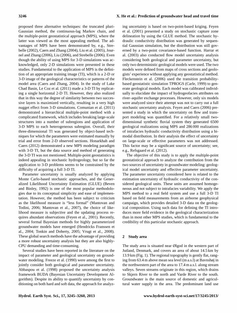
Fig. 1.Topography, stream network and observation stations aroundØlgod. “BoreholeShallow” are boreholes with bottom elevationhigher than−70 m a.s.l., while “BoreholeDeep” are boreholes withbottom elevation lower than−70 m a.s.l. The red line indicates thelocation of the cross section in Fig. 2.

is agriculture, which is featured by a well-developed sub-surface drainage system. Weather in this area is influencedby both the North Sea and the European continent. Theaverage annual temperature is 8.2◦C, with a maximum of16.5◦C in August and a minimum of 1.4◦C in January.The mean annual precipitation in the area is approximately1050 mm yr−1, with frequent intense rain in autumn andwinter and less rain in spring (Stisen et al., 2011).

2.1 Geology

The lower boundary of the aquifers in the area is consti-tuted by thick impermeable Paleogene clay deposited inhemipelagic environments and located at depths of 260–320 m (Høyer et al., 2013). The Paleogene clay is covered byMiocene clay, silt and sand deposits mainly originating fromdeltaic and shallow marine environments (Rasmussen et al.,2010). The thickness of these Miocene deposits increasesfrom east to west in the study area and attains thicknesses ofup to approximately 150 m. During the Pleistocene, phasesof erosion, deposition and deformation resulted in a highlyheterogeneous glaciotectonic complex above the Paleogeneand Miocene. Buried tunnel valleys were deeply incised andsubsequently filled, glacial and interglacial sediments weredeposited and the entire setting was finally heavily deformedby one or more glaciers in the Late Pleistocene (Jørgensenand Sandersen, 2006). The resulting Pleistocene sequence istherefore highly variable in thickness and ranges from 0 tomore than 300 m. Borehole data and seismic data collectedin the study area confirm a highly heterogeneous setting ofthe Pleistocene sediments above−100 m a.s.l. (Høyer et al.,2011). Groundwater reservoirs in this region are often found

Table 1.Observations of groundwater head and river flow.

Number of Standard ObservationObservations observations deviation period

Head Obs. 1 68 2 m 2009–2010Head Obs. 2 151 4 m 1960–2009River Flow 1 812 m3 d−1 1990–2005

in the Miocene sand deposits or within the heterogeneousPleistocene setting.

2.2 Data collection and processing

2.2.1 Geological and geophysical data

The three-dimensional geostatistical models developed inthe study are based on multiple data sources, includ-ing borehole description, seismic data and SkyTEM (air-borne transient electromagnetic method) data (Høyer et al.,2011). Borehole data are obtained from the Danish nationalgeological database JUPITER (http://www.geus.dk/jupiter/index-dk.htm). JUPITER contains over 240 000 boreholeswith information regarding geology, geography, hydrogeol-ogy, and groundwater chemistry. 525 boreholes with geolog-ical description are located within the study area; however,96 % of them are shallow wells with bottom elevation above−70 m a.s.l. (Fig. 1), and only 22 boreholes have data deeperthan−70 m a.s.l. In the subsequent analysis the geologicaldescriptions from JUPITER have been simplified and catego-rized into four main geological units: Quaternary sand, Qua-ternary clay, pre-Quaternary sand and pre-Quaternary clay.

2.2.2 Construction of training image (TI)

The training image was indirectly constructed from SkyTEMdata collected in the study area. The SkyTEM system(Sørensen and Auken, 2004) measures the electrical resis-tivity of the subsurface down to about−250 m, and this pa-rameter can be utilized for determining the clay content ifgroundwater salinity does not change considerably across thesurvey area. The data were collected with a flight line spacingof only 125 to 270 m (Høyer et al., 2011), providing a densedata coverage. Data processing and inversion is described inHøyer et al. (2011). For the conversion from electrical resis-tivity to clay content a geostatistical estimation concept in-volving borehole information and SkyTEM data was devel-oped (Jørgensen et al., 2012). This concept uses non-linearinversion to estimate clay content in all cells of a regular 3-Dgrid by optimizing a translator function for the conversion.The final result was a binary sand–clay model discretized ina regular 3-D grid covering the entire study area (Jørgensenet al., 2012).

www.hydrol-earth-syst-sci.net/17/3245/2013/ Hydrol. Earth Syst. Sci., 17, 3245–3260, 2013

http://www.geus.dk/jupiter/index-dk.htm

http://www.geus.dk/jupiter/index-dk.htm


2.2.3 Hydrological data

Two groups of hydraulic head data are available (Table 1).Group 1 includes 68 observations, which were obtained dur-ing the latest sampling campaigns in 2009 and 2010 (Alectia,2011), and Group 2 includes 151 observations retrieved fromthe JUPITER database. Group 1 data were considered to bemore accurate than Group 2 data, hence the standard devia-tion for the uncertainty of the two types of data was assumed2 and 4 m, respectively.

Stream discharge is only available from one station,Q25.32, located slightly outside the study area in the north-eastern part (Fig. 1). The topographical catchment area tothe station is around 64 km2. Based on the historical dailydata from 1990–2005, river discharge ranges from less than0.1 m3 s−1 during summer to more than 5.0 m3 s−1 dur-ing late autumn, and the 16 yr daily average discharge is0.8 m3 s−1 (69 000 m3 d−1).

Estimates of groundwater recharge are extracted from theDanish national water resources model, the DK-model (Hen-riksen et al., 2003). The net recharge (precipitation minus ac-tual evapotranspiration) varies between 0 to 2.5 mm d−1, andon average the net groundwater recharge in the model area iscomputed to 611 mm yr−1.

Groundwater abstraction data are extracted from theJUPITER database. 165 pumping wells for domestic use, ir-rigation, fish farms and industry consumption are located inthe study area, with a total abstraction of 3.2× 106 m3 yr−1

for the period 2000 to 2010.

3 Modeling methodology

3.1 Geostatistical simulation

An important part of this study is the generation of stochas-tic geological models using the multiple-point geostatisti-cal approach (MPS) (Guardiano and Srivastava, 1993; Stre-belle, 2002; Journel and Zhang, 2006), which has been in-tegrated in the Stanford Geostatistical Modeling Software(SGeMS) (Remy et al., 2009). We apply the single normalequation simulation algorithm (SNESIM) (Strebelle, 2002)of MPS, which has reconciled the strengths of traditionalobject-based and pixel-based simulation algorithms (Liu etal., 2005). Object-based geostatistics is advantageous in cap-turing spatial pattern and structure but encounters difficultywhen conditioned to large amounts of local data. In con-trast, traditional pixel-based algorithms honor local data byreproducing a variogram or covariance model with two-pointstatistics, and in this process it eludes the geostatistical infor-mation concealed in large-scale patterns. The newly devel-oped pixel-based algorithm, SNESIM, maintains the flexibil-ity of data conditioning and directly collects the probabilitydistribution from a training image (TI) with multiple points,hereby overcoming the limitation of two-point geostatistics.

Geostatistical simulations primarily depend on the condi-tional probability distribution function (cpdf). In SNESIM,the cpdf is set equal to the corresponding training imageproportions (Strebelle, 2002). This training proportion is ob-tained by scanning one or several training images (TI) witha multiple-node training template. The classical sequentialsimulation paradigm (Goovaerts, 1997, p. 376) is used todraw the stochastic images. The main step is to first assignhard data to the closest node of the simulation grid, while allthe unknown nodes are visited once and only once by a ran-dom path. At each unknown node, all the surrounding harddata presented within a certain search template are retainedas conditioning data events, with which the correspondingconditional probability is computed.

The crucial requisite of applying SNESIM is to providea TI which represents the geological characteristics of thestudy area. As the TI is the primary source of uncertaintywhen using MPS, an important step is to obtain the ap-propriate TI (Comunian et al., 2011). Previous applicationsof MPS have mostly been constrained to 2-D TIs (Caers,2001; Strebelle, 2002; Comunian et al., 2012). In this studywe use the 3-D training image mainly based on the de-tailed geophysical data collected during the flight campaign(Jørgensen et al., 2012).

3.2 Groundwater and optimization models

A steady-state groundwater flow model was constructed us-ing the groundwater modeling computer code MODFLOW-2000 (Harbaugh et al., 2000) within the framework of theGroundwater Modeling System (GMS). To enable an ac-curate representation of the geological heterogeneity in thestochastic realizations, the Hydrogeologic-Unit Flow (HUF)package (Evan and Mary, 2000) was used. The HUF packageallows the vertical stratigraphy to be defined independentlyof the numerical model layers by using hydrogeologic units.For the groundwater flow process, the HUF package com-putes the hydraulic properties of the model grid according tothe hydrogeologic units within the model grid. The cell-to-cell flow conductance in horizontal and vertical directions iscalculated as the arithmetic and harmonic mean, respectively,as discussed by McDonald and Harbaugh (1988). Other ac-tivated packages are specified head, recharge (RCH), river(RIV), drain (DRT) and well (WEL).

Although several advanced inverse modeling methodsbased on global search algorithms have been presented re-cently, they are mostly quite time-consuming. Since we onlyfocus on hydraulic conductivities for steady-state flow con-ditions, advanced algorithms designed for multi-objectiveoptimizations are not required. Instead, we use the Model-independent parameter estimation & uncertainty analysis(PEST) inversion code (Doherty, 2005) for parameter es-timation and for parameter sensitivity assessment. PESTuses a local search algorithm and has the advantage of fastconvergence. Additionally, besides estimating the optimum



parameter (Brauchler et al., 2007; Cheng and Chen, 2007;Baalousha, 2012), we also considered the equifinality of dif-ferent parameter sets by sampling within parameters’ distri-bution space.

Based on the flow solutions generated by MODFLOW, theparticle-tracking post-processing code MODPATH (David,1994) was used to simulate particle travel time distributions.The backward particle tracking option simulates the path-ways of particles from a certain cell to the possible corre-sponding groundwater recharge points reversely along theflow direction. By sampling the group of particles in a cell,one can compute the probability distribution of travel timeusing basic statistical analysis.

3.3 Uncertainty analysis

The uncertainty associated with geological structure was an-alyzed by utilizing 100 stochastic geological realizationsgenerated by SNESIM as input to MODFLOW. To distin-guish between parameter and geological uncertainty, threescenarios were defined:

Scenario 1: GeoModel-I: In the first scenario fixed hy-draulic parameters were specified for the individual ge-ological units for all MODFLOW models. The param-eter values were taken as the median of the values ob-tained by calibration of each individual model.

Scenario 2: GeoModel-II: In this scenario each modelwas calibrated by PEST. The parameters included in theoptimization were horizontal hydraulic conductivity ofQuaternary sand, Quaternary clay and pre-Quaternarysand.

Scenario 3: GeoParModel: In the third scenario param-eter uncertainty was added. Each MODFLOW modelbased on GeoModel-II was subject to a stochastic pa-rameter analysis. Only the uncertainty of the hydraulicconductivity of Quaternary sand, Quaternary clay andpre-Quaternary sand was considered, since the sensitiv-ity analysis documented that the groundwater flow sim-ulations were mostly sensitive to these parameters.

In the analysis, the uncertainty of hydraulic conductivity wasassumed to be log-normally distributed (Freeze, 1975; Hoek-sema and Kitanidis, 1985). The variation of hydraulic con-ductivity between the realizations was generated based onthe optimization results, where the optimized values repre-sent the mean values and the standard deviations are derivedfrom the 95 % confidence intervals (CI) estimated by PEST.

Random sampling in the parameter space was carried outusing the Latin hypercube approach (McKay et al., 1979).Latin Hypercube Sampling (LHS) is a stratified samplingmethod where the parameter spaceS is divided intoN seg-ments of equal marginal probability 1/N and sampled val-ues from different parameters are randomly combined. In

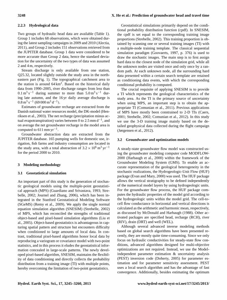
Fig. 2. Cross section with model grid and training image geolog-ical structure. Location on plain view is shown in Fig. 1. Verticalexaggeration is 15.

this way LHS captures the full parameter space in a simpli-fied manner and requires much fewer model runs comparedto normal random sampling. In our study, the distributionspace for each of the three hydraulic parameters was dividedinto six segments of equal probability, and therefore the to-tal number of simulations for each geological realization is63 = 216. We refer to the set of simulations for each geolog-ical realization based on sampling in the parameter space asParModel, while the ensemble of simulations for all geolog-ical realizations and all parameter variations (90× 216 sim-ulations in total) is referred to as GeoParModel.

For all scenarios backward particle tracking was appliedto four selected wells using MODPATH.

4 Groundwater model setup

4.1 Geological structure

The groundwater model extends from land surface to−300 m a.s.l., where the Paleogene clay occupies the wholearea and is therefore taken as lower boundary of the model(Fig. 2). The corresponding geological setup consists of twoparts. The upper part includes layers from the land surfaceto −70 m a.s.l. This part contains only heterogeneous Qua-ternary sediments and has abundant borehole data for condi-tioning simulation; hence this part is subject to the geosta-tistical simulations by SNESIM on a 100 m× 100 m× 5 mgrid. The lower part is generally dominated by comparablymore homogeneous pre-Quaternary sediments. The geolog-ical structure of the pre-Quaternary sediments is describedby a manual interpretation of mainly seismic data (Høyer etal., 2011; Jørgensen et al., 2012), since only few boreholesreach this deeper part and the SkyTEM data show limitedresolution capability here (Høyer et al., 2011). At the placeswhere Quaternary sediments are located between the pre-Quaternary surface and−70 m a.s.l., the geological model isdefined by the SkyTEM-based training image (Fig. 2).



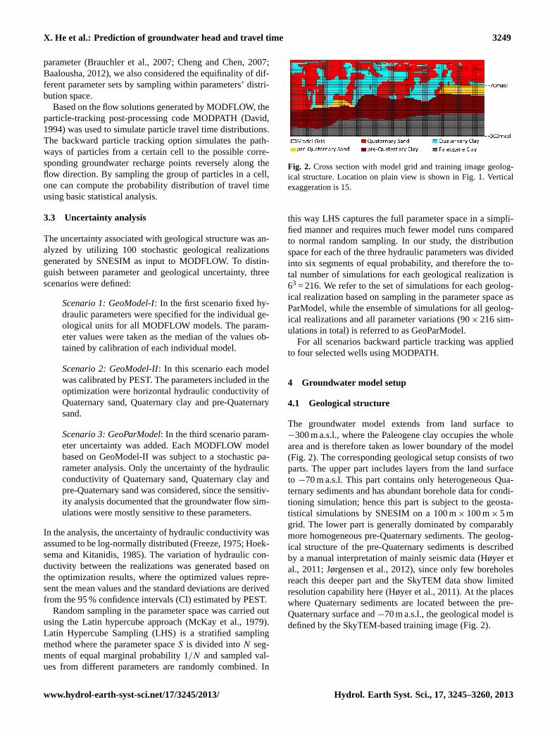
Fig. 3.Transition probability of Quaternary sediments.(a) Borehole data in lateral direction;(b) data from 3-D training image (TI) in lateraldirection;(c) borehole data in vertical direction;(d) data from 3-D TI in vertical direction.

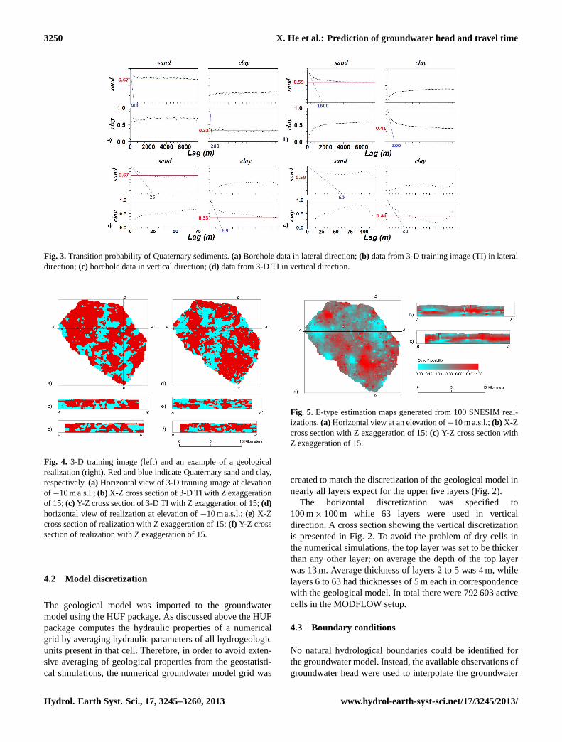
Fig. 4. 3-D training image (left) and an example of a geologicalrealization (right). Red and blue indicate Quaternary sand and clay,respectively.(a) Horizontal view of 3-D training image at elevationof −10 m a.s.l.;(b) X-Z cross section of 3-D TI with Z exaggerationof 15; (c) Y-Z cross section of 3-D TI with Z exaggeration of 15;(d)horizontal view of realization at elevation of−10 m a.s.l.;(e) X-Zcross section of realization with Z exaggeration of 15;(f) Y-Z crosssection of realization with Z exaggeration of 15.

4.2 Model discretization

The geological model was imported to the groundwatermodel using the HUF package. As discussed above the HUFpackage computes the hydraulic properties of a numericalgrid by averaging hydraulic parameters of all hydrogeologicunits present in that cell. Therefore, in order to avoid exten-sive averaging of geological properties from the geostatisti-cal simulations, the numerical groundwater model grid was

Fig. 5. E-type estimation maps generated from 100 SNESIM real-izations.(a) Horizontal view at an elevation of−10 m a.s.l.;(b) X-Zcross section with Z exaggeration of 15;(c) Y-Z cross section withZ exaggeration of 15.

created to match the discretization of the geological model innearly all layers expect for the upper five layers (Fig. 2).

The horizontal discretization was specified to100 m× 100 m while 63 layers were used in verticaldirection. A cross section showing the vertical discretizationis presented in Fig. 2. To avoid the problem of dry cells inthe numerical simulations, the top layer was set to be thickerthan any other layer; on average the depth of the top layerwas 13 m. Average thickness of layers 2 to 5 was 4 m, whilelayers 6 to 63 had thicknesses of 5 m each in correspondencewith the geological model. In total there were 792 603 activecells in the MODFLOW setup.

4.3 Boundary conditions

No natural hydrological boundaries could be identified forthe groundwater model. Instead, the available observations ofgroundwater head were used to interpolate the groundwater



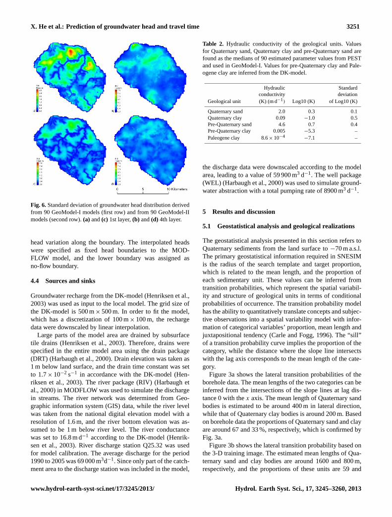
Fig. 6.Standard deviation of groundwater head distribution derivedfrom 90 GeoModel-I models (first row) and from 90 GeoModel-IImodels (second row).(a) and(c) 1st layer,(b) and(d) 4th layer.

head variation along the boundary. The interpolated headswere specified as fixed head boundaries to the MOD-FLOW model, and the lower boundary was assigned asno-flow boundary.

4.4 Sources and sinks

Groundwater recharge from the DK-model (Henriksen et al.,2003) was used as input to the local model. The grid size ofthe DK-model is 500 m× 500 m. In order to fit the model,which has a discretization of 100 m× 100 m, the rechargedata were downscaled by linear interpolation.

Large parts of the model area are drained by subsurfacetile drains (Henriksen et al., 2003). Therefore, drains werespecified in the entire model area using the drain package(DRT) (Harbaugh et al., 2000). Drain elevation was taken as1 m below land surface, and the drain time constant was setto 1.7× 10−2 s−1 in accordance with the DK-model (Hen-riksen et al., 2003). The river package (RIV) (Harbaugh etal., 2000) in MODFLOW was used to simulate the dischargein streams. The river network was determined from Geo-graphic information system (GIS) data, while the river levelwas taken from the national digital elevation model with aresolution of 1.6 m, and the river bottom elevation was as-sumed to be 1 m below river level. The river conductancewas set to 16.8 m d−1 according to the DK-model (Henrik-sen et al., 2003). River discharge station Q25.32 was usedfor model calibration. The average discharge for the period1990 to 2005 was 69 000 m3d−1. Since only part of the catch-ment area to the discharge station was included in the model,

Table 2. Hydraulic conductivity of the geological units. Valuesfor Quaternary sand, Quaternary clay and pre-Quaternary sand arefound as the medians of 90 estimated parameter values from PESTand used in GeoModel-I. Values for pre-Quaternary clay and Pale-ogene clay are inferred from the DK-model.

Hydraulic Standardconductivity deviation

Geological unit (K) (m d−1) Log10 (K) of Log10 (K)

Quaternary sand 2.0 0.3 0.1Quaternary clay 0.09 −1.0 0.5Pre-Quaternary sand 4.6 0.7 0.4Pre-Quaternary clay 0.005 −5.3 –Paleogene clay 8.6× 10−4

−7.1 –

the discharge data were downscaled according to the modelarea, leading to a value of 59 900 m3 d−1. The well package(WEL) (Harbaugh et al., 2000) was used to simulate ground-water abstraction with a total pumping rate of 8900 m3 d−1.

5 Results and discussion

5.1 Geostatistical analysis and geological realizations

The geostatistical analysis presented in this section refers toQuaternary sediments from the land surface to−70 m a.s.l.The primary geostatistical information required in SNESIMis the radius of the search template and target proportion,which is related to the mean length, and the proportion ofeach sedimentary unit. These values can be inferred fromtransition probabilities, which represent the spatial variabil-ity and structure of geological units in terms of conditionalprobabilities of occurrence. The transition probability modelhas the ability to quantitatively translate concepts and subjec-tive observations into a spatial variability model with infor-mation of categorical variables’ proportion, mean length andjuxtapositional tendency (Carle and Fogg, 1996). The “sill”of a transition probability curve implies the proportion of thecategory, while the distance where the slope line intersectswith the lag axis corresponds to the mean length of the cate-gory.

Figure 3a shows the lateral transition probabilities of theborehole data. The mean lengths of the two categories can beinferred from the intersections of the slope lines at lag dis-tance 0 with thex axis. The mean length of Quaternary sandbodies is estimated to be around 400 m in lateral direction,while that of Quaternary clay bodies is around 200 m. Basedon borehole data the proportions of Quaternary sand and clayare around 67 and 33 %, respectively, which is confirmed byFig. 3a.

Figure 3b shows the lateral transition probability based onthe 3-D training image. The estimated mean lengths of Qua-ternary sand and clay bodies are around 1600 and 800 m,respectively, and the proportions of these units are 59 and



Table 3. Travel time based on backward particle tracking for four wells for GeoModel-I, GeoModel-II, GeoParModel, and median of Par-Models.R denotes the fraction of the 95 % confidence interval to the one from GeoParModel. Location of the four wells is shown in Fig. 8.

W1 W2 W3 W4

GeoModel-I

Median (year) 50 29 46 3195 % Interval (year) 29 34 171 14R 91 % 83 % 87 % 70 %Skewness 0.3 1.6 2.3 6.0

GeoModel-II


GeoParModel


Median of 90 ParModels

Median (year) 52 31 48 3195 % Interval (year) 6 5 21 5R 18 % 12 % 11 % 26 %Skewness 1.1 0.4 −0.4 −0.1

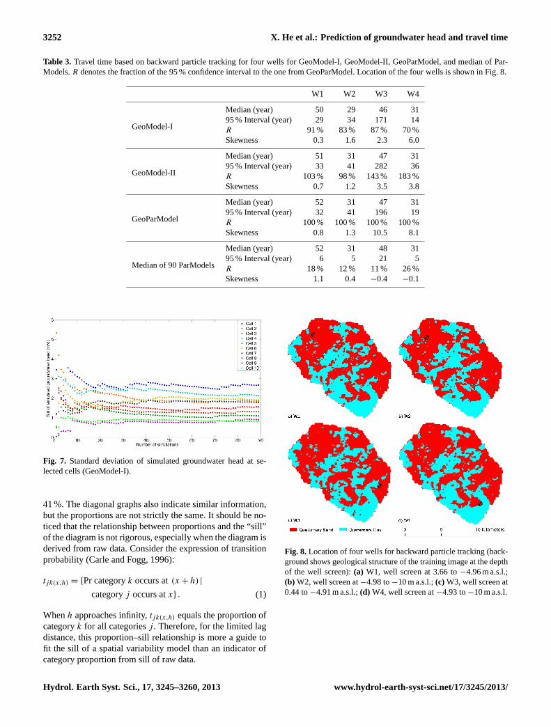
Fig. 7. Standard deviation of simulated groundwater head at se-lected cells (GeoModel-I).

41 %. The diagonal graphs also indicate similar information,but the proportions are not strictly the same. It should be no-ticed that the relationship between proportions and the “sill”of the diagram is not rigorous, especially when the diagram isderived from raw data. Consider the expression of transitionprobability (Carle and Fogg, 1996):

tjk(x,h) = {Pr categoryk occurs at(x + h) |

categoryj occurs atx} . (1)

Whenh approaches infinity,tjk(x,h) equals the proportion ofcategoryk for all categoriesj . Therefore, for the limited lagdistance, this proportion–sill relationship is more a guide tofit the sill of a spatial variability model than an indicator ofcategory proportion from sill of raw data.

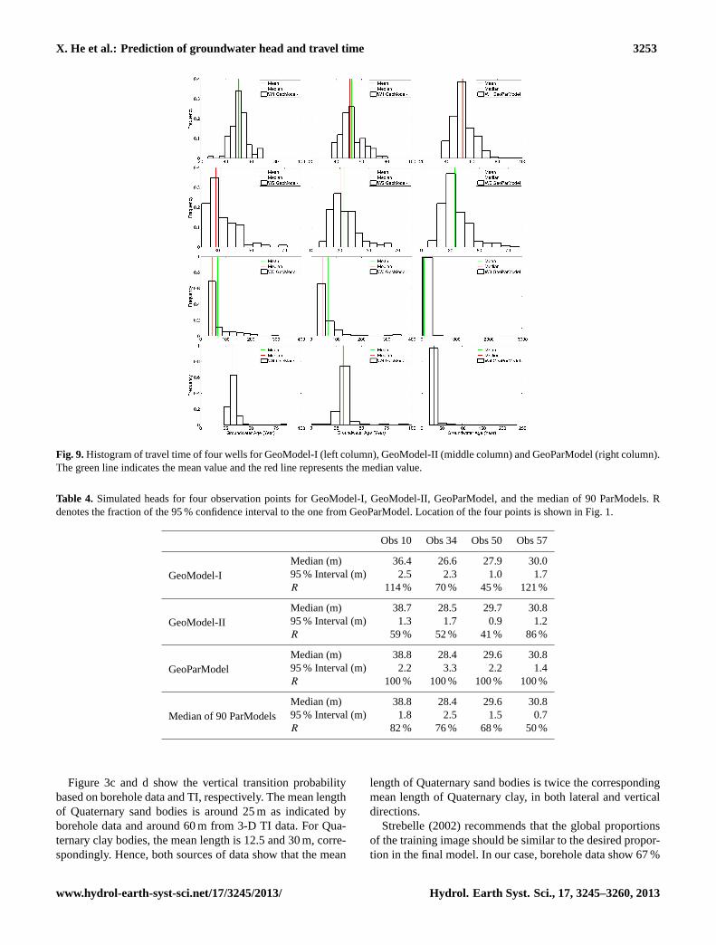
Fig. 8.Location of four wells for backward particle tracking (back-ground shows geological structure of the training image at the depthof the well screen):(a) W1, well screen at 3.66 to−4.96 m a.s.l.;(b) W2, well screen at−4.98 to−10 m a.s.l.;(c) W3, well screen at0.44 to−4.91 m a.s.l.;(d) W4, well screen at−4.93 to−10 m a.s.l.



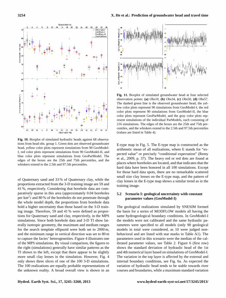
Fig. 9.Histogram of travel time of four wells for GeoModel-I (left column), GeoModel-II (middle column) and GeoParModel (right column).The green line indicates the mean value and the red line represents the median value.

Table 4. Simulated heads for four observation points for GeoModel-I, GeoModel-II, GeoParModel, and the median of 90 ParModels. Rdenotes the fraction of the 95 % confidence interval to the one from GeoParModel. Location of the four points is shown in Fig. 1.

Obs 10 Obs 34 Obs 50 Obs 57

GeoModel-IMedian (m) 36.4 26.6 27.9 30.095 % Interval (m) 2.5 2.3 1.0 1.7R 114 % 70 % 45 % 121 %

GeoModel-IIMedian (m) 38.7 28.5 29.7 30.895 % Interval (m) 1.3 1.7 0.9 1.2R 59 % 52 % 41 % 86 %

GeoParModelMedian (m) 38.8 28.4 29.6 30.895 % Interval (m) 2.2 3.3 2.2 1.4R 100 % 100 % 100 % 100 %

Median of 90 ParModelsMedian (m) 38.8 28.4 29.6 30.895 % Interval (m) 1.8 2.5 1.5 0.7R 82 % 76 % 68 % 50 %

Figure 3c and d show the vertical transition probabilitybased on borehole data and TI, respectively. The mean lengthof Quaternary sand bodies is around 25 m as indicated byborehole data and around 60 m from 3-D TI data. For Qua-ternary clay bodies, the mean length is 12.5 and 30 m, corre-spondingly. Hence, both sources of data show that the mean

length of Quaternary sand bodies is twice the correspondingmean length of Quaternary clay, in both lateral and verticaldirections.

Strebelle (2002) recommends that the global proportionsof the training image should be similar to the desired propor-tion in the final model. In our case, borehole data show 67 %



41

1

Fig. 10. Boxplot of simulated hydraulic heads against 68 observations from head obs. group 1. 2

Green dots are observed groundwater head, yellow color plots represent simulations from 90 3

GeoModel-I, red color plots represent simulations from 90 GeoModel-II, and blue color plots 4

represent simulations from GeoParModel. The edges of the boxes are the 25th

and 75th

5

percentiles, and the whiskers extend to the 2.5th

and 97.5th

percentiles. 6

7

Fig. 10.Boxplot of simulated hydraulic heads against 68 observa-tions from head obs. group 1. Green dots are observed groundwaterhead, yellow color plots represent simulations from 90 GeoModel-I, red color plots represent simulations from 90 GeoModel-II, andblue color plots represent simulations from GeoParModel. Theedges of the boxes are the 25th and 75th percentiles, and thewhiskers extend to the 2.5th and 97.5th percentiles.

of Quaternary sand and 33 % of Quaternary clay, while theproportions extracted from the 3-D training image are 59 and41 %, respectively. Considering that borehole data are com-paratively sparse in this area (approximately 0.04 boreholesper km2) and 80 % of the boreholes do not penetrate throughthe whole model depth, the proportions from borehole datahold a higher uncertainty than those based on the 3-D train-ing image. Therefore, 59 and 41 % were defined as propor-tions for Quaternary sand and clay, respectively, in the MPSsimulations. Since both borehole data and 3-D TI show lat-erally isotropic geometry, the maximum and medium rangesfor the search template ellipsoid were both set to 2000 m,and the minimum range in vertical direction was set to 80 mto capture the facies’ heterogeneities. Figure 4 illustrates oneof the MPS simulations. By visual comparison, the figures tothe right (simulations) generally have similar patterns as theTI shown to the left, except that there appear to be slightlymore small clay lenses in the simulation. However, Fig. 4only shows three slices of one of the 100 3-D simulations.The 100 realizations are equally probable representations ofthe unknown reality. A broad overall view is shown in an

Fig. 11. Boxplot of simulated groundwater head at four selectedobservation points:(a) Obs10,(b) Obs34,(c) Obs50,(d) Obs57.The dashed green line is the observed groundwater head, the yel-low color plots represent 90 simulations from GeoModel-I, the redcolor plots represent 90 simulations from GeoModel-II, the bluecolor plots represent GeoParModel, and the gray color plots rep-resent simulations of the individual ParModels, each consisting of216 simulations. The edges of the boxes are the 25th and 75th per-centiles, and the whiskers extend to the 2.5th and 97.5th percentiles(values are listed in Table 4).

E-type map in Fig. 5. The E-type map is constructed as thearithmetic mean of all realizations, where E stands for “ex-pected value” or precisely “conditional expectation” (Remyet al., 2009, p. 37). The heavy red or red dots are found atplaces where boreholes are located, and that indicates that thehard data have been honored in all 100 simulations. Exceptfor those hard data spots, there are no remarkable scatteredsmall size clay lenses on the E-type map, and the pattern ofclay lenses in the E-type map shows a similar trend as in thetraining image.

5.2 Scenario I: geological uncertainty with constantparameter values (GeoModel-I)

The geological realizations simulated by SNESIM formedthe basis for a series of MODFLOW models all having thesame hydrogeological boundary conditions. In GeoModel-Ithe models were not calibrated and the same hydraulic pa-rameters were specified to all models (only 90 geologicalmodels in total were considered, as 10 were judged non-behavioral and are listed with star marks in Table A1). Theparameters used in this scenario were the median of the cal-ibrated parameter values, see Table 2. Figure 6 (first row)shows the standard deviation of hydraulic head of the 1stand 4th numerical layer based on simulations of GeoModel-I.The variation in the top layer is affected by the external andinternal boundary conditions, see Fig. 6a. As expected thevariation of hydraulic head tends to be stable towards rivercourses and boundaries, while a maximum standard variation



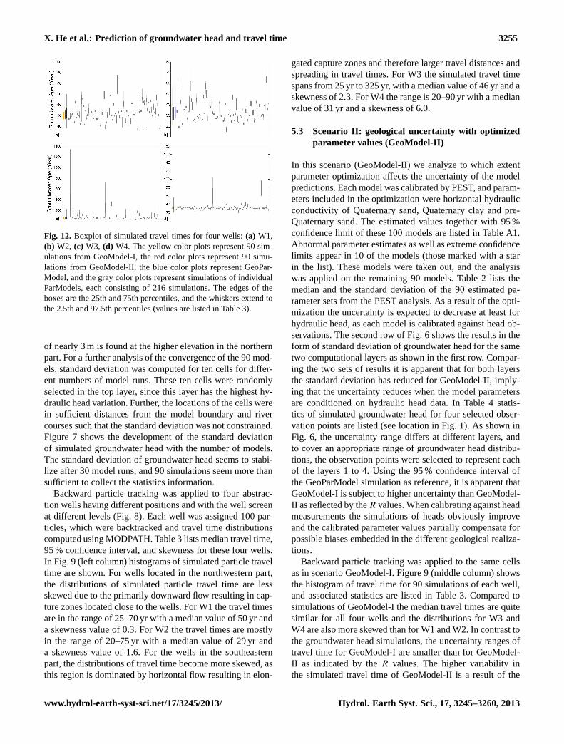
Fig. 12. Boxplot of simulated travel times for four wells:(a) W1,(b) W2, (c) W3, (d) W4. The yellow color plots represent 90 sim-ulations from GeoModel-I, the red color plots represent 90 simu-lations from GeoModel-II, the blue color plots represent GeoPar-Model, and the gray color plots represent simulations of individualParModels, each consisting of 216 simulations. The edges of theboxes are the 25th and 75th percentiles, and the whiskers extend tothe 2.5th and 97.5th percentiles (values are listed in Table 3).

of nearly 3 m is found at the higher elevation in the northernpart. For a further analysis of the convergence of the 90 mod-els, standard deviation was computed for ten cells for differ-ent numbers of model runs. These ten cells were randomlyselected in the top layer, since this layer has the highest hy-draulic head variation. Further, the locations of the cells werein sufficient distances from the model boundary and rivercourses such that the standard deviation was not constrained.Figure 7 shows the development of the standard deviationof simulated groundwater head with the number of models.The standard deviation of groundwater head seems to stabi-lize after 30 model runs, and 90 simulations seem more thansufficient to collect the statistics information.

Backward particle tracking was applied to four abstrac-tion wells having different positions and with the well screenat different levels (Fig. 8). Each well was assigned 100 par-ticles, which were backtracked and travel time distributionscomputed using MODPATH. Table 3 lists median travel time,95 % confidence interval, and skewness for these four wells.In Fig. 9 (left column) histograms of simulated particle traveltime are shown. For wells located in the northwestern part,the distributions of simulated particle travel time are lessskewed due to the primarily downward flow resulting in cap-ture zones located close to the wells. For W1 the travel timesare in the range of 25–70 yr with a median value of 50 yr anda skewness value of 0.3. For W2 the travel times are mostlyin the range of 20–75 yr with a median value of 29 yr anda skewness value of 1.6. For the wells in the southeasternpart, the distributions of travel time become more skewed, asthis region is dominated by horizontal flow resulting in elon-

gated capture zones and therefore larger travel distances andspreading in travel times. For W3 the simulated travel timespans from 25 yr to 325 yr, with a median value of 46 yr and askewness of 2.3. For W4 the range is 20–90 yr with a medianvalue of 31 yr and a skewness of 6.0.

5.3 Scenario II: geological uncertainty with optimizedparameter values (GeoModel-II)

In this scenario (GeoModel-II) we analyze to which extentparameter optimization affects the uncertainty of the modelpredictions. Each model was calibrated by PEST, and param-eters included in the optimization were horizontal hydraulicconductivity of Quaternary sand, Quaternary clay and pre-Quaternary sand. The estimated values together with 95 %confidence limit of these 100 models are listed in Table A1.Abnormal parameter estimates as well as extreme confidencelimits appear in 10 of the models (those marked with a starin the list). These models were taken out, and the analysiswas applied on the remaining 90 models. Table 2 lists themedian and the standard deviation of the 90 estimated pa-rameter sets from the PEST analysis. As a result of the opti-mization the uncertainty is expected to decrease at least forhydraulic head, as each model is calibrated against head ob-servations. The second row of Fig. 6 shows the results in theform of standard deviation of groundwater head for the sametwo computational layers as shown in the first row. Compar-ing the two sets of results it is apparent that for both layersthe standard deviation has reduced for GeoModel-II, imply-ing that the uncertainty reduces when the model parametersare conditioned on hydraulic head data. In Table 4 statis-tics of simulated groundwater head for four selected obser-vation points are listed (see location in Fig. 1). As shown inFig. 6, the uncertainty range differs at different layers, andto cover an appropriate range of groundwater head distribu-tions, the observation points were selected to represent eachof the layers 1 to 4. Using the 95 % confidence interval ofthe GeoParModel simulation as reference, it is apparent thatGeoModel-I is subject to higher uncertainty than GeoModel-II as reflected by theR values. When calibrating against headmeasurements the simulations of heads obviously improveand the calibrated parameter values partially compensate forpossible biases embedded in the different geological realiza-tions.

Backward particle tracking was applied to the same cellsas in scenario GeoModel-I. Figure 9 (middle column) showsthe histogram of travel time for 90 simulations of each well,and associated statistics are listed in Table 3. Compared tosimulations of GeoModel-I the median travel times are quitesimilar for all four wells and the distributions for W3 andW4 are also more skewed than for W1 and W2. In contrast tothe groundwater head simulations, the uncertainty ranges oftravel time for GeoModel-I are smaller than for GeoModel-II as indicated by theR values. The higher variability inthe simulated travel time of GeoModel-II is a result of the



calibration process. When calibrating against head measure-ments the resulting variation in parameter values gives riseto a higher variability in flow pathlines and velocities, andrealizations with extreme travel time are introduced. Similarresults were obtained by Refsgaard et al. (2012).

5.4 Scenario III: geological and parameter uncertainty(ParModel and GeoParModel)

The parameters included in the parameter uncertainty anal-ysis were the same three parameters which were optimizedby the PEST code in the previous scenarios. For each ofthe 90 models developed in the GeoModel-II scenario, 216parameter sets were sampled and each sampled parameterset served as input to MODFLOW simulations. Figure 10shows boxplots of the distribution of simulated heads basedon GeoModel-I, GeoModel-II, and GeoParModel for each ofthe 68 observation points from Head Obs. Group 1 in Ta-ble 1. The edges of the boxes represent the 25th and 75thpercentiles, while the whiskers extend to the 2.5th and 97.5thpercentiles, respectively. The observed groundwater headsfor each well are shown by green dots. The simulations basedon GeoModel-I (yellow boxes) are generally lower than thecorresponding observations. This bias is a result of the im-posed constant parameter values. As expected, the resultsfrom GeoModel-II are in better agreement with observationsand the associated uncertainties (red boxes) are less than forGeoModel-I. When parameter uncertainty is added repre-sented by GeoParModel (blue boxes) the uncertainty of thesimulated heads is increased and is higher compared to thetwo other scenarios.

To illustrate the impact of parameter uncertainty explic-itly, boxplots for heads at four randomly selected observationpoints (same as in Table 4) are shown in Fig. 11. The greendashed lines in the figures represent the observed groundwa-ter heads, while the yellow, red and blue boxplots representthe same scenarios as in Fig. 10. The gray boxplots show theresults from the ParModels. As stated above, each ParModelrepresents the results of 216 simulations, which are generatedfrom random sampling in the parameter spaces derived fromthe PEST analysis of each GeoModel-II. The median valuesand 95 % uncertainty ranges for all scenarios for these fourpoints are listed in Table 4. The results listed in the last rowof the table are the median values of the results of all the 90ParModels, i.e., median of the medians and 95 % intervals.We take these results as a representation of the impact of pa-rameter uncertainty. Using the uncertainty range of GeoPar-Model as reference, theR values for the GeoModel-II aremuch lower than 100 %, indicating that the uncertainty fromGeoModel-II is less than that from GeoParModel. The differ-ence between the two scenarios is that parameter uncertaintyhas been added to GeoParModel, suggesting that uncertaintyon hydraulic head is increased when parameter uncertaintyis considered. The median values of the 90 ParModels listedin Table 4 show that the median of the uncertainty intervals

of all 90 ParModels is slightly higher than the correspondinginterval for GeoModel-II for three of the observation points.This suggests that the effect of parameter uncertainty is com-parable to the effect of geological uncertainty with respect tohydraulic head uncertainty.

Backward particle tracking was applied to the 216 param-eter realizations of each ParModel. The travel time distribu-tion of 90× 216 realizations is plotted in Fig. 9 (right col-umn), and the corresponding values of median, 95 % intervaland skewness are listed in Table 3. By introducing parame-ter uncertainty in the GeoParModel, the uncertainty rangesof travel time have increased somewhat, as more extremetravel times are found when comparing the right and mid-dle columns of Fig. 9. However, this is not necessarily re-flected in theR values. TheR values are computed fromthe 95 % confidence intervals and when the skewness is notcomparable between the scenarios as for W3 and W4, theR values may be misleading. Nevertheless, in contrast to hy-draulic head simulation, parameter uncertainty has much lesseffect on travel time simulation. This can be inferred from thevery lowR values based on the median of the 90 ParModelsand also evidenced from the boxplots of the individual Par-Model simulations shown in Fig. 12. Although there are afew outliers, overall the uncertainty intervals of the individ-ual ParModels are generally shorter than the correspondingintervals for GeoModel-I and GeoModel-II, suggesting thatthe effect of parameter uncertainty is relatively low with re-spect to travel time. In this regard the geological architectureis the most critical factor.

6 Conclusions

This study has examined the impact of geological and pa-rameter uncertainty on real case simulations of groundwaterheads and travel time using the multiple-point geostatisticalmethod (MPS). A 3-D training image derived from geophys-ical data was used as basis for the MPS simulations. Usuallygeophysical data are used as soft data for conditioning; how-ever, as used here it was possible to develop a reliable 3-Dgeological model as a training image input to the MPS.

Generally one would expect that the uncertainty rangewill decrease when calibrating models, but our results showthat this is not always the case. Although the uncertainty ofgroundwater head simulations is reduced when the parame-ters are calibrated against hydraulic head observations, theopposite is the case for the uncertainty of travel time simu-lations. Calibration implies that biases in the realizations ofgeological architecture are compensated by errors in param-eter values which lead to a larger range of variation in traveltime. This also underpins previous findings that when usingmodels outside the calibrated regime, which indeed is thecase when simulating travel time, the prediction uncertaintyis high.



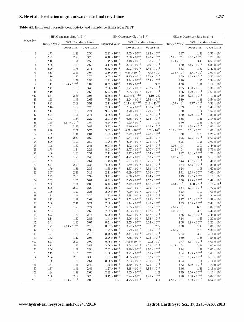
Table A1. Estimated hydraulic conductivity and confidence limits from PEST.

Model No.HK Quaternary Sand (m d−1) HK Quaternary Clay (m d−1) HK pre-Quaternary Sand (m d−1)

Estimated Value95 % Confidence Limits



Lower Limit Upper Limit Lower Limit Upper Limit Lower Limit Upper Limit

1 1.75 1.23 2.50 2.25× 10−1 5.65× 10−2 8.92× 10−1 5.37 1.23 2.36× 101

2 2.93 2.28 3.76 6.10× 10−2 2.60× 10−2 1.43× 10−1 9.91× 10−1 5.62× 10−3 1.75× 102

3 2.10 1.71 2.58 1.49× 10−2 3.18× 10−3 6.98× 10−2 1.71× 101 3.43 8.55× 101

4 2.06 1.63 2.60 3.11× 10−2 3.03× 10−3 3.19× 10−1 1.30 2.46× 10−2 6.89× 101

5 2.20 1.78 2.71 6.52× 10−2 2.92× 10−2 1.45× 10−1 6.63 1.82 2.42× 101

*6 3.13 2.66 3.67 2.16× 10−5 6.30× 10−20 7.43× 109 2.33× 102 2.71× 101 2.01× 103

7 2.16 1.70 2.76 9.57× 10−2 4.15× 10−2 2.21× 10−1 3.59 3.63× 10−1 3.55× 101

8 1.94 1.51 2.50 1.21× 10−1 5.34× 10−2 2.72× 10−1 6.10 1.47 2.54× 101

9 1.11 6.49× 10−1 1.89 8.57× 10−1 2.19× 10−1 3.35 4.50 1.71 1.19× 101

10 2.41 1.68 3.46 7.06× 10−2 1.71× 10−2 2.92× 10−1 1.05 4.80× 10−3 2.31× 102

11 2.19 1.82 2.63 6.73× 10−2 2.65× 10−2 1.71× 10−1 1.86 1.29× 10−1 2.69× 101

*12 3.34 2.81 3.96 8.39× 10−6 6.39× 10−253 1.10+242 8.29 6.22× 10−1 1.11× 102

13 1.95 1.43 2.65 7.59× 10−2 2.24× 10−2 2.56× 10−1 5.30 1.11 2.54× 101

*14 3.25 2.69 3.91 2.11× 10−7 2.11× 10−307 2.11× 10293 4.57× 102 3.77× 101 5.53× 103

15 2.16 1.69 2.76 7.30× 10−2 2.84× 10−2 1.88× 10−1 5.39 1.16 2.49× 101

16 2.12 1.65 2.71 9.22× 10−2 3.70× 10−2 2.29× 10−1 6.30 1.54 2.57× 101

17 2.27 1.91 2.71 3.89× 10−2 5.11× 10−3 2.97× 10−1 1.80 1.79× 10−1 1.81× 101

18 1.73 1.34 2.22 2.01× 10−1 6.56× 10−2 6.14× 10−1 4.88 1.11 2.14× 101

19 1.29 8.87× 10−1 1.87 4.54× 10−1 1.23× 10−1 1.67 6.46 2.29 1.82× 101

20 2.82 2.27 3.49 5.92× 10−2 2.16× 10−2 1.62× 10−1 2.21 1.74× 10−1 2.80× 101

*21 3.28 2.87 3.75 3.92× 10−5 6.58× 10−35 2.33× 1025 6.19× 10−1 3.61× 10−4 1.06× 103

22 1.99 1.41 2.81 1.83× 10−1 7.47× 10−2 4.48× 10−1 6.30 1.73 2.29× 101

23 2.99 2.49 3.60 1.81× 10−2 5.44× 10−3 6.02× 10−2 3.05 1.65× 10−1 5.61× 101

24 2.00 1.57 2.55 1.26× 10−1 4.79× 10−2 3.31× 10−1 4.95 1.21 2.03× 101

25 1.95 1.57 2.41 9.91× 10−2 4.02× 10−2 2.45× 10−1 1.03× 101 3.07 3.44× 101

26 1.75 1.34 2.29 8.01× 10−2 3.77× 10−2 1.70× 10−1 2.18× 101 8.29 5.73× 101

27 1.80 1.30 2.51 2.11× 10−1 5.17× 10−2 8.64× 10−1 2.97 7.31× 10−1 1.21× 101

28 2.09 1.78 2.46 2.13× 10−2 4.71× 10−3 9.63× 10−2 1.03× 101 3.41 3.13× 101

29 2.05 1.59 2.64 1.45× 10−1 5.61× 10−2 3.75× 10−1 2.44 4.07× 10−1 1.46× 101

30 2.77 2.29 3.36 4.06× 10−2 1.49× 10−2 1.11× 10−1 2.64 3.83× 10−1 1.81× 101

31 1.79 1.36 2.35 1.55× 10−1 4.37× 10−2 5.51× 10−1 4.24 1.08 1.67× 101

32 2.67 2.23 3.18 2.11× 10−2 6.29× 10−3 7.06× 10−2 2.91 1.68× 10−1 5.05× 101

33 2.47 2.05 2.99 3.41× 10−2 6.68× 10−3 1.74× 10−1 1.19 1.22× 10−2 1.17× 102

34 2.39 1.86 3.07 6.21× 10−2 2.45× 10−2 1.57× 10−1 3.20 4.23× 10−1 2.42× 101

35 2.20 1.71 2.83 6.43× 10−3 2.47× 10−4 1.67× 10−1 4.84× 102 1.98× 101 1.18× 104

36 2.58 2.08 3.20 3.72× 10−2 1.77× 10−2 7.80× 10−2 3.44 2.51× 10−1 4.72× 101

37 1.69 1.29 2.21 2.06× 10−1 7.09× 10−2 6.00× 10−1 4.23 1.08 1.66× 101

38 1.81 1.41 2.32 1.53× 10−1 5.35× 10−2 4.35× 10−1 5.96 1.61 2.21× 101

39 2.12 1.68 2.69 9.02× 10−2 2.72× 10−2 2.99× 10−1 3.27 6.72× 10−1 1.59× 101

40 2.60 2.11 3.21 2.88× 10−2 1.14× 10−2 7.28× 10−2 4.33 2.53× 10−1 7.43× 101

41 2.21 1.79 2.74 2.27× 10−2 5.95× 10−3 8.67× 10−2 2.62× 101 6.39 1.07× 102

42 2.03 1.58 2.60 7.55× 10−2 3.53× 10−2 1.62× 10−1 1.05× 101 3.23 3.40× 101

43 2.23 1.80 2.76 5.90× 10−2 2.22× 10−2 1.57× 10−1 2.76 2.21× 10−1 3.45× 101

44 2.14 1.60 2.86 1.41× 10−1 5.06× 10−2 3.93× 10−1 7.14 1.55 3.30× 101

45 2.41 1.90 3.07 8.51× 10−2 3.55× 10−2 2.04× 10−1 2.08 1.95× 10−1 2.22× 101

46 1.23 7.18× 10−1 2.10 8.01× 10−1 3.22× 10−1 2.52 3.38 1.13 1.01× 101

47 2.33 1.85 2.93 1.75× 10−2 5.79× 10−3 5.31× 10−2 2.62× 101 7.36 9.30× 101

48 1.71 1.36 2.16 8.46× 10−2 3.41× 10−2 2.10× 10−1 9.84 3.09 3.14× 101

49 1.52 1.12 2.05 2.26× 10−1 7.58× 10−2 6.72× 10−1 4.60 1.38 1.54× 101

*50 2.63 2.28 3.02 8.79× 10−5 3.65× 10−13 2.12× 104 5.77 3.85× 10−1 8.66× 101

51 2.12 1.79 2.53 2.96× 10−2 7.24× 10−3 1.21× 10−1 1.13× 101 3.21 4.00× 101

52 2.06 1.68 2.54 7.03× 10−2 3.30× 10−2 1.50× 10−1 5.84 1.71 2.00× 101

53 2.13 1.65 2.76 1.08× 10−1 3.21× 10−2 3.61× 10−1 2.64 4.29× 10−1 1.63× 101

54 2.84 2.39 3.36 1.81× 10−2 4.95× 10−3 6.62× 10−2 5.31 8.85× 10−1 3.19× 101

55 1.90 1.39 2.61 8.20× 10−2 2.93× 10−2 2.30× 10−1 4.64 1.01 2.14× 101

56 1.87 1.41 2.49 1.48× 10−1 3.80× 10−2 5.75× 10−1 3.72 8.09× 10−1 1.71× 101

57 1.87 1.41 2.49 1.27× 10−1 4.18× 10−2 3.85× 10−1 5.46 1.36 2.19× 101

58 1.84 1.29 2.60 2.39× 10−1 5.65× 10−2 1.01 2.49 5.60× 10−1 1.11× 101

59 2.60 2.07 3.26 3.19× 10−2 7.24× 10−3 1.41× 10−1 1.20 2.88× 10−2 5.04× 101

*60 1.27 7.93× 10−1 2.03 1.35 4.75× 10−1 3.81 4.98× 10−1 3.80× 10−3 6.54× 101



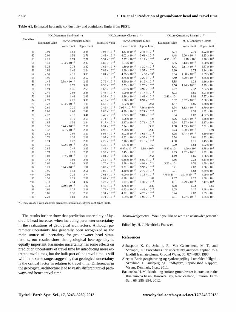
Table A1. Estimated hydraulic conductivity and confidence limits from PEST.

ModelNo.HK Quaternary Sand (m d−1) HK Quaternary Clay (m d−1) HK pre-Quaternary Sand (m d−1)




Lower Limit Upper Limit Lower Limit Upper Limit Lower Limit Upper Limit

61 1.92 1.54 2.38 1.03× 10−1 4.37× 10−2 2.43× 10−1 7.94 2.16 2.92× 101

62 2.04 1.53 2.71 1.48× 10−1 6.02× 10−2 3.63× 10−1 4.48 9.00× 10−1 2.23× 101

63 2.20 1.74 2.77 5.54× 10−3 2.77× 10−4 1.11× 10−1 4.55× 102 1.18× 101 1.76× 104

64 1.49 9.54× 10−1 2.32 4.89× 10−1 1.53× 10−1 1.56 2.85 8.13× 10−1 1.00× 101

65 3.26 2.78 3.82 1.62× 10−2 1.89× 10−3 1.39× 10−1 3.43 2.11× 10−1 5.57× 101

66 1.82 1.48 2.24 7.83× 10−2 3.90× 10−2 1.57× 10−1 9.30 2.75 3.14× 101

67 2.59 2.19 3.05 1.04× 10−3 4.25× 10−9 2.57× 102 2.64 4.38× 10−2 1.59× 102

68 1.95 1.52 2.52 1.10× 10−1 3.75× 10−2 3.20× 10−1 5.40 8.20× 10−1 3.55× 101

69 1.45 9.58× 10−1 2.19 2.79× 10−1 8.50× 10−2 9.19× 10−1 3.85 1.28 1.16× 101

70 2.28 1.73 3.02 6.56× 10−2 2.53× 10−2 1.70× 10−1 2.56 1.24× 10−1 5.29× 101

71 1.91 1.36 2.69 1.67× 10−1 6.97× 10−2 3.99× 10−1 7.67 2.32 2.54× 101

72 2.40 2.03 2.85 3.43× 10−2 1.00× 10−2 1.17× 10−1 8.03 1.65 3.91× 101

73 1.89 1.43 2.49 6.38× 10−2 2.86× 10−2 1.43× 10−1 2.46× 101 8.03 7.57× 101

74 2.78 2.28 3.39 4.18× 10−2 1.96× 10−2 8.91× 10−2 3.82 5.62× 10−1 2.60× 101

75 1.22 7.54× 10−1 1.98 6.50× 10−1 1.62× 10−1 2.61 4.87 1.86 1.28× 101

*76 2.60 2.29 2.95 2.42× 10−6 7.95× 10−115 7.36× 10102 1.74 1.12× 10−1 2.70× 101

77 2.00 1.62 2.46 9.80× 10−2 4.29× 10−2 2.24× 10−1 4.92 1.33 1.82× 101

78 2.72 2.17 3.41 3.45× 10−2 1.32× 10−2 9.01× 10−2 6.54 1.07 4.02× 101

79 1.74 1.19 2.53 3.71× 10−1 1.08× 10−1 1.28 3.26 8.25× 10−1 1.28× 101

80 1.88 1.52 2.34 8.17× 10−2 2.47× 10−2 2.71× 10−1 4.24 8.27× 10−1 2.17× 101

81 1.36 8.44× 10−1 2.18 8.34× 10−1 2.74× 10−1 3.18 1.88 1.53× 10−1 2.31× 101

82 1.37 8.71× 10−1 2.14 6.92× 10−1 2.08× 10−1 2.30 2.73 8.30× 10−1 8.9983 2.52 2.04 3.10 6.98× 10−2 3.02× 10−2 1.61× 10−1 3.28 3.47× 10−1 3.10× 101

84 1.70 1.33 2.18 1.97× 10−1 8.92× 10−2 4.35× 10−1 9.54 3.61 2.52× 101

85 1.74 1.27 2.38 2.26× 10−1 7.16× 10−2 7.16× 10−1 4.00 1.11 1.45× 101

86 1.35 8.72× 10−1 2.08 5.39× 10−1 1.87× 10−1 1.55 5.29 1.84 1.52× 101

*87 2.85 2.47 3.29 1.42× 10−5 6.97× 10−30 2.88× 1019 8.47× 101 1.90× 101 3.78× 102

88 1.77 1.23 2.55 2.98× 10−1 7.45× 10−2 1.19 2.93 7.02× 10−1 1.22× 101

89 1.03 5.57× 10−1 1.89 7.01× 10−1 1.96× 10−1 2.51 4.19 1.65 1.06× 101

90 1.43 1.01 2.01 2.52× 10−1 9.36× 10−2 6.80× 10−1 6.86 2.23 2.11× 101

91 2.60 2.09 3.23 1.70× 10−2 5.88× 10−3 4.91× 10−2 3.26× 101 6.70 1.59× 102

92 1.29 8.74× 10−1 1.91 3.02× 10−1 9.21× 10−2 9.93× 10−1 6.21 2.07 1.86× 101

93 1.95 1.51 2.51 1.05× 10−1 4.10× 10−2 2.70× 10−1 6.61 1.83 2.39× 101

*94 2.92 2.28 3.74 2.61× 10−2 6.00× 10−3 1.14× 10−1 7.78× 10−1 1.01× 10−10 5.99× 109

95 1.58 1.21 2.07 2.62× 10−1 6.78× 10−2 1.01 4.37 1.27 1.50× 101

*96 3.18 2.54 3.97 5.23× 10−2 1.97× 10−2 1.39× 10−1 1.31 2.29× 10−5 7.47× 104

97 1.13 6.60× 10−1 1.95 8.40× 10−1 2.76× 10−1 3.20 3.58 1.33 9.6598 1.64 1.27 2.11 1.74× 10−1 6.73× 10−2 4.48× 10−1 8.05 2.17 2.98× 101

99 1.86 1.38 2.50 1.34× 10−1 4.22× 10−2 4.25× 10−1 6.24 2.07 1.89× 101

100 2.28 1.81 2.88 5.74× 10−2 1.69× 10−2 1.95× 10−1 2.81 4.27× 10−1 1.85× 101

* Denotes models with abnormal parameter estimates or extreme confidence limits.

The results further show that prediction uncertainty of hy-draulic head increases when including parameter uncertaintyin the realizations of geological architecture. Although pa-rameter uncertainty has generally been recognized as themain source of uncertainty for groundwater head simu-lations, our results show that geological heterogeneity isequally important. Parameter uncertainty has some effects onprediction uncertainty of travel time by introducing more ex-treme travel times, but the bulk part of the travel time is stillwithin the same range, suggesting that geological uncertaintyis the critical factor in relation to travel time. Differences inthe geological architecture lead to vastly different travel path-ways and hence travel time.

Acknowledgements.Would you like to write an acknowledgement?

Edited by: H.-J. Hendricks Franssen

References

Abbaspour, K. C., Schulin, R., Van Genuchtena, M. T., andSchlappi, E.: Procedures for uncertainty analyses applied to alandfill leachate plume, Ground Water, 36, 874–883, 1998.

Alectia: Boringsregistrering og synkronpejling I omradet “Ølgod-Skovlund + Krusbjerg og Lindbjerg”, unpublished Rapport,Virum, Denmark, 5 pp., 2011.

Baalousha, H. M.: Modelling surface-groundwater interaction in theRuataniwha basin, Hawke’s Bay, New Zealand, Environ. EarthSci., 66, 285–294, 2012.



Beven, K. J. and Binley, A.: The future of distributed models: modelcalibration and uncertainty prediction, Hydrol. Process., 6, 279–298, 1992.

Brauchler, R., Cheng, J. T., Dietrich, P., Everett, M., Johnson, B.,Liedl, R., and Sauter, M.: An inversion strategy for hydraulic to-mography: coupling travel time and amplitude inversion, J. Hy-drol., 345, 184–198, 2007.

Caers, J.: Geostatistical reservoir modeling using statistical patternrecognition, J. Petrol. Sci. Eng., 29, 177–188, 2001.

Caers, J. and Zhang, T.: Multiple-point geostatistics: a quantitativevehicle for integrating geologic analogs into multiple reservoirmodels, in: AAPG Special Volumes Memoir 80: Integration ofOutcrop and Modern Analogs in Reservoir Modeling, edited by:Grammer, G. M., Harris, P. M., and Eberli, G. P., Tulsa, OK,USA, 383–394, 2004.

Carle, S. F. And Fogg, G. E.: Transition Probability-Based IndicatorGeostatistics, Mathe. Geol., 28, 453–476, 1996.

Carle, S. F.: TPROGS – Transition Probability Geostatistical Soft-ware, Version 2.1, User Manual, Hydrologic Sciences GraduateGroup, University of California, Davis, California, 1999.

Carle, S. F., LaBolle, E. M., Weissmann, G. S., VanBrocklin, D.,and Fogg, G. E.: Conditional simulation of hydrofacies archi-tecture: a transition probability/Markov approach, in: Hydroge-ologic Models of Sedimentary Aquifers, Concepts in Hydroge-ology and Environmental Geology No. 1, edited by: Fraser, G.S. and Davis, J. M., SEPM (Society for Sedimentary Geology)Special Publication, AAPG, Tulsa, OK, USA, 147–170, 1998.

Cheng, C. and Chen, X. H.: Evaluation of methods for determina-tion of hydraulic properties in an aquifer-aquitard system hydro-logically connected to a river, Hydrogeol. J., 15, 669–678, 2007.

Comunian, A., Renard, P., Straubhaar, J., and Bayer, P.: Three-dimensional high resolution fluvio-glacial aquifer analog, Part 2:Geostatistical modelling, J. Hydrol., 405, 10–23, 2011.

Comunian, A., Renard, P., and Straubhaar, J.: 3-D multiple-pointstatistics simulation using 2-D training images, Comput. Geosci.,40, 49–65, 2012.

David, W. P.: User’s Guide for MODPATH/MODPATH-PLOT, Ver-sion 3: a Particle Tracking Post-Processing Package for MOD-FLOW, the US Geological Survey Finite-Difference Ground-Water Flow Model, US Geological Survey Open File Rep. 94–464, Tulsa, OK, USA, 1994.

Delhomme, J. P.: Spatial variability and uncertainty in groundwaterflow parameters: a geostatistical approach, Water Resour. Res.,15, 269–280, 1979.

Dettinger, M. D. and Wilson, J. L.: First order analysis of uncer-tainty in numerical models of groundwater flow, Water Resour.Res., 17, 149–161, 1981.

Doherty, J.: PEST: Model Independent Parameter Estimation, 5thEdn. of user manual, Watermark Numerical Computing, Bris-bane, Australia, 2005.

Evan, R. A. and Mary, C. H.: Documentation of the hydrogeologic-unit flow (HUF) package, US Geological Survey Open File Rep.00–342, US Geological Survey, Denver, CO, USA, 2000.

Feyen, L. and Caers, J.: Quantifying geological uncertainty for flowand transport modeling in multi-modal heterogeneous forma-tions, Adv. Water Resour., 29, 912–929, 2006.

Feyen, L., Beven, K. J., De Smedt, F., and Freer, J.: Stochasticcapture zone delineation within the generalized likelihood un-certainty estimation methodology: conditioning on head obser-

vations, Water Resour. Res., 37, 625–638, 2001.Fleckenstein, J. H., Niswonger, R. G., and Fogg, G. E.: River-

aquifer interactions, geologic heterogeneity, and low-flow man-agement, Ground Water, 44, 837–852, 2006.

Freeze, R. A.: A stochastic-conceptual analysis of one-dimensionalgroundwater flow in nonuniform homogeneous media, Water Re-sour. Res., 11, 725–741, 1975.

Freeze, R. A., Massmann, J., Smith, L., Sperling, T., and James,B.: Hydrogeological decision analysis: 1. A framework, GroundWater, 28, 738–766, 1990.

Goovaerts, P.: Geostatistics for Natural Resources Evaluation, Ox-ford University Press, New York, 483 pp., 1997.

Guardiano, F. and Srivastava, R. M.: Multivariate geostatistics:beyond bivariate moments: geostatistics-troia, in: Geostatistics-Troia, Vol. 1, edited by: Soares, A., Kluwer, Dordrecht, 133–144,1993.

Harbaugh, A. W., Banta, E. R., Hill, M. C., and McDonald, M. G.:MODFLOW-2000, the US Geological Survey Modular Ground-Water Model – User Guide to Modularization Concepts and theGround-Water Flow Process, US Geological Survey Open-FileReport 00–92, US Department of Interior, Reston, VA, USA,121 pp., 2000.

Harrar, W. G., Sonnenborg, T. O., and Henriksen, H. J.: Capturezone, travel time, and solute transport predictions using inversemodeling and different geological models, J. Hydrol., 11, 536–548, 2003.

Hassan, A.E, Bekhit, H. M., and Chapman, J. B.: Uncertainty as-sessment of a stochastic groundwater flow model using GLUEanalysis, J. Hydrol., 362, 89–109, 2008.

Henriksen, H. J., Troldborg, L., Nyegaard, P., Sonnenborg, T. O.,Refsgaard, J. C., and Madsen, B.: Methodology for construction,calibration and validation of a national hydrological model forDenmark, J. Hydrol., 280, 52–71, 2003.

Hendricks Franssen, H. J., Stauffer, F., and Kinzelbach, W.: Joint es-timation of transmissivities and recharges–application: stochasticcharacterization of well capture zones, J. Hydrol., 294, 87–102,2004.

Hoeksema, R. J. and Kitanidis, P. K.: Analysis of the spatial struc-ture of properties of selected aquifers, Water Resour. Res., 21,563–572, 1985.

Honarkhah, M. and Caers, J.: Direct Pattern-Based Simulation ofNonstationary Geostatistical Models, Math. Geosci., 44, 651–672, 2012.

Høyer, A. S., Lykke-Andersen, H., Jørgensen, F., andAuken, E.: Combined interpretation of SkyTEM and high-resolution seismic data, Phys. Chem. Earth, 36, 1386–1397,doi:10.1016/j.pce.2011.01.001, 2011.

Høyer, A. S., Jørgensen, F., Lykke-Andersen, H., and Christiansen,A. V.: Iterative modelling of AEM data based on geological apriori information from seismic and borehole data, Near Surf.Geophys., submitted, 2013.

Johnson, N. M.: Characterization of alluvial hydrostratigraphy withindicator semivariograms, Water Resour. Res., 31, 3205–3216,1995.

Journel, A. G.: Beyond covariance: the advent of multiple-pointgeostatistics, in: Geostatistics, Banff, edited by: Leuangthong, O.and Deutsch, C. V., Springer, Dordrecht, The Netherlands, 2004,225–233, 2005.


http://dx.doi.org/10.1016/j.pce.2011.01.001


Journel, A. G. and Alabert, F.: New method for reservoir mapping,J. Petrol. Technol., 42, 212–218, 1990.

Journel, A. G. and Zhang, T.: The necessity of a multiplepoint priormodel, Math. Geol., 38, 591–610, 2006.

Jørgensen, F. and Sandersen, P. B. E.: Buried and open tunnel val-leys in Denmark – erosion beneath multiple ice sheets, Quater-nary Sci. Rev., 25, 1339–1363, 2006.

Jørgensen, F., Møller, R. R., Høyer, A. H., and Christiansen, A.V.: Geologisk model ved Ølgod og Skovlund – eksempel p°aeffektiviseret modellering i et heterogent geologisk miljø, Dan-marks og Grønlands Geologiske Undersøgelse Rapport 2012/82,GEUS, Copenhagen, Denmark, 83 pp., 2012.

Klise, K. A., Weissmann, G. S., McKenna, S. A., Nichols,E. M., Frechette, J. D., Wawrzyniec, T. F., and Tidwell, V.C.: Exploring solute transport and streamline connectivity us-ing Lidar-based outcrop images and geostatistical represen-tations of heterogeneity, Water Resour. Res., 45, W05413,doi:10.1029/2008WR007500, 2009.

Le Coz, M., Genthon, P., and Adler, P. M.: Multiple-point statis-tics for modeling facies heterogeneities in a porous medium: theKomadugu-Yobe Alluvium, Lake Chad Basin, Math. Geosci., 43,861–878, 2011.

Liu, Y.: Using the Snesim program for multiple-point statistical sim-ulation, Comput. Geosci., 32, 1544–1563, 2006.

Liu, Y., Harding, A., Journel, A. G., and Gilbert, R.: A workflow formultiple-point geostatistical simulation, in: Geostatistics Banff2004, Vol. 1, edited by: Leuangthong, O. and Deutsch, C. V.,Springer, Dordrecht, 245–254, 2005.

Mariethoz, G., Renard, P., Cornaton, F., and Jaquet, O.: TruncatedPlurigaussian simulations to characterize aquifer heterogeneity,Ground Water, 47, 13–24, 2009.

McDonald, M. G. and Harbaugh, A. W.: A Modular Three-Dimensional Finite-Difference Ground-Water Flow Model, USGeological Survey Open File Rep. 83–875, US GPO, Washing-ton, USA, 1988.

McKay, M. D., Conover, W. J., and Beckman, R. J.: A comparisonof three methods for selection values of input variables in theanalysis of output from a computer code, Technometrics, 2, 239–245, 1979.

Mantovan, P. and Todini, E.: Hydrological forecasting uncertaintyassessment: incoherence of the GLUE methodology, J. Hydrol.,330, 368–381, 2006.

Mantovan, P., Todini, E., and Martina, M. L. V.: Reply to com-ment by Keith Beven, Paul Smith and Jim Freer on “Hydrologi-cal forecasting uncertainty assessment: incoherence of the GLUEmethodology”, J. Hydrol., 228, 319–324, 2007.

Rasmussen, E. S., Dybkjær, K., and Piasecki, S.: Lithostratigraphyof the Upper Oligocene Miocene Succession of Denmark, Geo-logical Survey of Denmark and Greenland Bulletin, 22, GEUS,Copenhagen, Denmark, 92 pp., 2010.

Refsgaard, J. C., Christensen, S., Sonnenborg, D. S., Hojberg, A. L.,and Troldborg, L.: Review of strategies for handling geologicaluncertainty in groundwater flow and transport modeling, Adv.Water Resour., 36, 36–50, 2012.

Remy, N., Boucher, A., and Wu, J.: Applied Geostatistics withSGeMS, Cambridge University Press, Cambridge, UK, 2009.

Renard, P.: Stochastic hydrogeology: what professionals reallyneed?, Ground Water, 45, 531–541, 2007.

Sørensen, K. I. and Auken, E.: SkyTEM – a new high-resolutionhelicopter transient electromagnetic system, Explor. Geophys.,35, 191–199, 2004.

Stisen, S., Sonnenborg, T. O., Højberg, A. L., Troldborg, L., andRefsgaard, J. C.: Evaluation of climate input biases and waterbalance issues using a coupled surface-subsurface model, VadoseZone J., 10, 37–53, 2011.

Strebelle, S. B.: Conditional simulation of complex geologicalstructures using multiple-point statistics, Math. Geol., 34, 1–21,2002.

Strebelle, S. B.: Sequential simulation for modeling geologicalstructures from training images, in: Stochastic Modeling andGeostatistics: Principles, Methods, and Case Studies, vol. II:AAPG Computer Applications in Geology 5, edited by: Coburn,T. C., Yarus, J. M., and Chambers, R. L., AAPG, Tulsa, OK,USA, 139–149, 2006.

Tonkin, M. and Doherty, J.: A hybrid regularized inversion method-ology for highly parameterized environmental models, Water Re-sour. Res., 41, W10412, doi:10.1029/2005WR003995, 2005.

Vrugt, J. A., Stauffer, P. H., Wohling, T., Robinson, B. A., and Ves-selinov, V. V.: Inverse modeling of subsurface flow and transportproperties: a review with new developments, Vadose Zone J., 7,843–864, 2008.

Webb, E. K. and Anderson, M. P.: Simulation of preferential flow inthree-dimensional, heterogeneous conductivity fields with realis-tic internal architecture, Water Resour. Res., 32, 533–545, 1996.

Wingle, W. L. and Poeter, E. P.: Uncertainty associated with semi-variograms used for site simulation, Ground Water, 31, 725–734,1993.


http://dx.doi.org/10.1029/2008WR007500

http://dx.doi.org/10.1029/2005WR003995

Documents

Analyzing the effects of geological and parameter uncertainty on prediction of groundwater head