Ancient feeding, ecology and extinction of Pleistocene ...digital.csic.es/bitstream/10261/12306/1/Apa 1174.-427-436Sánchez... · During the Plio-Pleistocene, ... Animals then incorporate

Introduction

The Equidae family in South America is repre-sented by two genera, Hippidion and Equus (Amer-hippus). Both genera can be differentiated by theirsmall and large forms, probably as a consequence of

having adapted to similar environments. These im-migrant genera dispersed into South America usingtwo different routes. During the Plio-Pleistocene,two corridors developed that shaped the paleobio-geographic history of most of the North Americanmammals in South America (Webb, 1991). The mostviable model postulated for the horse’s dispersalprocess seems to indicate that the small forms uti-lized the Andes corridor, while larger horses dis-persed through the Eastern route and through somecoastal areas. The Pampean Region represents themost austral distribution for large horses that dis-persed through the Eastern route, while the group ofsmall horses that arrived as far as the southern

AMEGHINIANA (Rev. Asoc. Paleontol. Argent.) - 43 (2): 427-436. Buenos Aires, 30-6-2006 ISSN 0002-7014

©Asociación Paleontológica Argentina AMGHB2-0002-7014/06$00.00+.50

1Museo Nacional de Ciencias Naturales, CSIC, José GutiérrezAbascal, 2, 28006 Madrid, Spain. [email protected] and [email protected], Departamento de Arqueología, Universidad Na-cional del Centro, Del Valle 5737, 7400 Olavarría, Argentina. [email protected]

Ancient feeding, ecology and extinction of Pleistocenehorses from the Pampean Region, Argentina

Begoña SÁNCHEZ1, José Luis PRADO2 and María Teresa ALBERDI1

Key words. Equus (Amerhippus). Hippidion. Paleodiet. Ecology. Extinction. Pleistocene. Pampean region. SouthAmerica.

Palabras clave. Equus (Amerhippus). Hippidion. Paleodieta. Ecología. Extinción. Pleistoceno. Región Pampeana.América del Sur.

Abstract. To reconstruct the diet and habitat preference of fossil horses, we measured the carbon and oxygen isotopecomposition of 35 bone and tooth samples of Equus (Amerhippus) neogeus Lund, Hippidion principale (Lund), andHippidion devillei (Gervais) from 10 different Pleistocene localities in the Pampean region (Argentina). To compare thethree species by stratigraphic age, we divided the samples into three groups: lower Pleistocene, middle-late Pleistoceneand latest Pleistocene. Samples of Hippidion devillei from the lower Pleistocene were more homogeneous, with δ13C val-ues ranging between -11.73 to -9.79‰. These data indicate a diet exclusively dominated by C3 plants. In contrast,Hippidion principale and Equus (Amerhippus) neogeus from middle-late Pleistocene showed a wide range of feeding adap-tations (with a range of δ13C values between -12.05 to -8.08 ‰ in Hippidion and δ13C values between -11.46 to -7.21 ‰in Equus (Amerhippus)). These data seem to indicate a mixed C3 - C4 diet, while data from the latest Pleistocene suggesta tendency toward an exclusively C3 diet for both species. Furthermore, the results of δ18O indicate an increase of ap-proximately 4ºC from the early to latest Pleistocene in this area. Several nutritional hypotheses explaining latestPleistocene extinctions are based on the assumption that extinct taxa had specialized diets. The resource partitioningpreference of these species from latest Pleistocene in the Pampean region supports these hypotheses.

Resumen. PALEODIETA, ECOLOGÍA Y EXTINCIÓN DE LOS CABALLOS DEL PLEISTOCENO DE LA REGIÓN PAMPEANA, ARGENTINA. Paracomprender las variaciones en la dieta de los équidos, hemos analizado la composición isotópica del oxígeno y del car-bono del carbonato en 35 restos fósiles de Equus (Amerhippus) neogeus Lund, Hippidion principale (Lund) e Hippidion de-villei (Gervais) procedentes de 10 localidades del Pleistoceno de la Región Pampeana (Argentina). Para poder compa-rar las variaciones temporales de los resultados isotópicos, hemos agrupado las muestras según su procedencia estra-tigráfica en tres grupos: Pleistoceno inferior, Pleistoceno medio y superior y Pleistoceno tardío. Los datos indican quelas muestras del Pleistoceno temprano de Hippidion devillei son las más homogéneas, con un rango de variación de losvalores de δ13C entre -11,73 y -9,79‰. Estos resultados sugieren una dieta compuesta exclusivamente por plantas C3.Por el contrario los resultados de las muestras de Hippidion principale y Equus (Amerhippus) neogeus del Pleistoceno me-dio y superior presentan un mayor rango de variación (con valores de δ13C entre -12,05 y -8,08 ‰ para Hippidion y va-lores de δ13C entre -11,46 y -7,21 ‰ para Equus). Estos resultados indican una adaptación a una dieta mixta C3-C4. Porsu parte los especímenes del Pleistoceno tardío muestran nuevamente una tendencia hacia una dieta compuesta exclu-sivamente por plantas de tipo C3 para ambas especies. Además, los resultados de δ18O registran un aumento en la tem-peratura de alrededor 4 ºC en el área de estudio desde el inicio del Pleistoceno hasta el final. Algunos autores sugierenque un estrés nutricional, producto de un cambio rápido en las comunidades vegetales, podría ser una de las causasque expliquen la extinción del final del Pleistoceno. La especialización que observamos en la dieta en los caballos delfinal del Pleistoceno podría ser una evidencia en favor de esta teoría.

B. Sánchez, J.L. Prado and M.T. Alberdi428

Patagonia dispersed via the Western route. The dis-persal route of each form seems to reflect an adaptiveshift in their ecology (Alberdi and Prado, 1992;Alberdi et al., 1995). Recently, a similar pattern of dis-persion in South America was postulated for gom-photheres (Sánchez et al., 2004).

Horses have been recorded in the PampeanRegion from the late Pliocene to the latest Pleistocene(Alberdi and Prado, 1993; Prado and Alberdi, 1994).Three species are recognized: Equus (Amerhippus)neogeus Lund, 1840, Hippidion principale (Lund, 1846),and Hippidion devillei (Gervais, 1855).

In this paper we compare the results of carbonand oxygen isotopic composition from tooth, enamel,dentine and bone of these three species of equids, inorder to determine the paleodiet and habitat prefer-ences of Pleistocene horses in the Pampean Region,and show how variations in these preferences mayhave been related to their extinction.

Isotopic background

Previous studies have shown that the carbon iso-tope ratio (δ13C) of fossil teeth and bones can be usedto obtain dietary information about extinct herbi-vores (De Niro and Epstein, 1978; Vogel, 1978; Su-llivan and Krueger, 1981; Lee-Thorp et al., 1989, 1994;Koch et al., 1990, 1994; Quade et al., 1992; Cerling etal., 1997; MacFadden, 2000). This carbon isotope ratiois influenced by the type of plant material ingested,which is in turn influenced by the photosyntheticpathway utilized by the plants. During photosynthe-sis, C3 plants in terrestrial ecosystems (trees, bushes,shrubs, forbs, and high elevation and high latitudegrasses) discriminate more markedly against theheavy 13C isotope during fixation of CO2 than dotropical grasses and sedges (C4 plants). Thus, C3 andC4 plants have different δ13C values. C3 plants haveδ13C values of -22 per mil (‰) to -30‰, with an ave-rage of approximately -26‰, whereas C4 plants haveδ13 C values of -10 to -14‰, with an average of about-12‰ (Smith and Epstein, 1971; Vogel et al., 1978;Ehleringer et al., 1986, 1991; Cerling et al., 1993).Animals then incorporate carbon from food into theirtooth and bone with an additional fractionation of 12to 14‰. Mammals feeding on C3 plants (fruit, leaves,etc.) characteristically have δ13C values betweenabout -10 and -16‰, while animals that eat C4 tropi-cal grasses (including blades, seeds, and roots) haveδ13C values between +2 and -2‰. A mixed-feederwould fall somewhere in between these two ex-tremes (Lee-Thorp and van der Merwe, 1987; Quadeet al., 1992). Hence, the relative proportions of C3 andC4 vegetation in an animal diet can be determined byanalyzing its teeth and bone δ13C.

In recent decades, there has been an increasinguse of oxygen and carbon isotope analyses to recon-struct paleoenvironmental and paleoclimatical con-ditions. In the case of homeothermic animals in gen-eral, the oxygen isotope composition of apatite de-pends primarily on the oxygen balance of the animal(Longinelli, 1984; Luz et al., 1984). Influxes of oxy-gen include ingested water (drinking water + waterfrom plants) as well as inspired O2 gas; oxygen islost from the body as liquid water in urine, sweat,and feces, and as CO2 and H2O in respiratory gases.Factors acting on this balance are both internal (re-lated to the physiology of the animal) and external(related to ecology and to climate). Oxygen isotopevariations in large mammals depend largely on ex-ternal factors such as the δ18O of ingested water.Because the oxygen isotopic composition of phos-phate in mammalian bones and teeth (δ18Op) is relat-ed to that of ingested water, and ingested watercomes ultimately from precipitation, the δ18O ofenamel and bone phosphate can be used to infer pastclimatic conditions (Longinelli and Nuti, 1973;Kolodny et al., 1983; D’Angela and Longinelli, 1990;Bryant et al., 1994; Sánchez et al., 1994; Bryant andFroelich, 1995; Delgado et al., 1995; Kohn, 1996; Kohnet al., 1996, 1998).

Material and methods

Sampled area. The Pampa Plains contains extensiveformations of superficial sand and loess that areknown as the Pampean Formation (Teruggi, 1957).Paleomagnetic stratigraphy and radiometric datasuggest that most of this formation was depositedover the last 3.3 Ma. (Schultz et al., 1998). The strati-graphy of pampean loess typically consists of super-posed beds, 1-2 m thick, separated by either erosionaldiscontinuities or palaeosols. The majority of thesepalaeo-aeolian features lie in areas presently sup-porting vegetation communities dominated by grass-land. Most of the late Pleistocene and Holocene de-posits were assigned to either the Luján Formation(including three members: La Chumbiada, Guerreroand Río Salado) or to the La Postrera Formation (Fidal-go et al., 1973, 1975, 1991; Dillon and Rabassa, 1985).Luján deposits are fluvial-lacustrine and those of LaPostrera are eolian. The eolian deposits, which coverextensive parts of the southern Pampean Region, arecomprised of sandy loess, very fine sand sheets, anddunefields (Zárate and Blasi, 1993).

At present, the Pampean plains has a subtropicalclimate, wich varies from humid in the east to arid inthe west. This climatic pattern reflects the dominanteffects of the ocean in the southern half of SouthAmerica (Iriondo and García, 1993). The mean annu-

AMEGHINIANA 43 (2), 2006

Ancient feeding of Pleistocene horses 429

al temperatures is approximately 17°C and mean an-nual precipitation is around 800 mm.

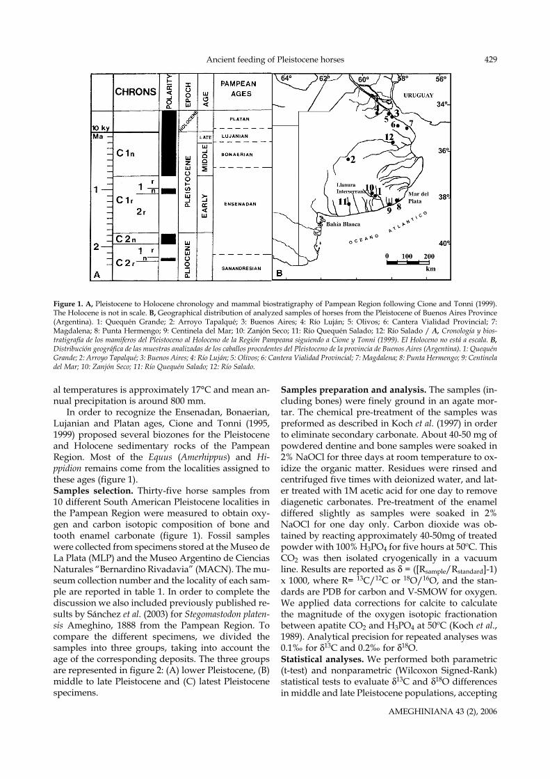
In order to recognize the Ensenadan, Bonaerian,Lujanian and Platan ages, Cione and Tonni (1995,1999) proposed several biozones for the Pleistoceneand Holocene sedimentary rocks of the PampeanRegion. Most of the Equus (Amerhippus) and Hi-ppidion remains come from the localities assigned tothese ages (figure 1). Samples selection. Thirty-five horse samples from10 different South American Pleistocene localities inthe Pampean Region were measured to obtain oxy-gen and carbon isotopic composition of bone andtooth enamel carbonate (figure 1). Fossil sampleswere collected from specimens stored at the Museo deLa Plata (MLP) and the Museo Argentino de CienciasNaturales “Bernardino Rivadavia” (MACN). The mu-seum collection number and the locality of each sam-ple are reported in table 1. In order to complete thediscussion we also included previously published re-sults by Sánchez et al. (2003) for Stegomastodon platen-sis Ameghino, 1888 from the Pampean Region. Tocompare the different specimens, we divided thesamples into three groups, taking into account theage of the corresponding deposits. The three groupsare represented in figure 2: (A) lower Pleistocene, (B)middle to late Pleistocene and (C) latest Pleistocenespecimens.

Samples preparation and analysis. The samples (in-cluding bones) were finely ground in an agate mor-tar. The chemical pre-treatment of the samples waspreformed as described in Koch et al. (1997) in orderto eliminate secondary carbonate. About 40-50 mg ofpowdered dentine and bone samples were soaked in2% NaOCl for three days at room temperature to ox-idize the organic matter. Residues were rinsed andcentrifuged five times with deionized water, and lat-er treated with 1M acetic acid for one day to removediagenetic carbonates. Pre-treatment of the enameldiffered slightly as samples were soaked in 2%NaOCl for one day only. Carbon dioxide was ob-tained by reacting approximately 40-50mg of treatedpowder with 100% H3PO4 for five hours at 50ºC. ThisCO2 was then isolated cryogenically in a vacuumline. Results are reported as δ = ([Rsample/Rstandard]-1)x 1000, where R= 13C/12C or 18O/16O, and the stan-dards are PDB for carbon and V-SMOW for oxygen.We applied data corrections for calcite to calculatethe magnitude of the oxygen isotopic fractionationbetween apatite CO2 and H3PO4 at 50ºC (Koch et al.,1989). Analytical precision for repeated analyses was0.1‰ for δ13C and 0.2‰ for δ18O.Statistical analyses. We performed both parametric(t-test) and nonparametric (Wilcoxon Signed-Rank)statistical tests to evaluate δ13C and δ18O differencesin middle and late Pleistocene populations, accepting


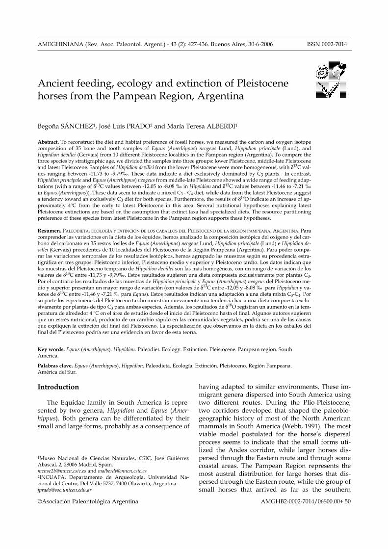
Figure 1. A, Pleistocene to Holocene chronology and mammal biostratigraphy of Pampean Region following Cione and Tonni (1999).The Holocene is not in scale. B, Geographical distribution of analyzed samples of horses from the Pleistocene of Buenos Aires Province(Argentina). 1: Quequén Grande; 2: Arroyo Tapalqué; 3: Buenos Aires; 4: Río Luján; 5: Olivos; 6: Cantera Vialidad Provincial; 7:Magdalena; 8: Punta Hermengo; 9: Centinela del Mar; 10: Zanjón Seco; 11: Río Quequén Salado; 12: Río Salado / A, Cronología y bios-tratigrafía de los mamíferos del Pleistoceno al Holoceno de la Región Pampeana siguiendo a Cione y Tonni (1999). El Holoceno no está a escala. B,Distribución geográfica de las muestras analizadas de los caballos procedentes del Pleistoceno de la provincia de Buenos Aires (Argentina). 1: QuequénGrande; 2: Arroyo Tapalqué; 3: Buenos Aires; 4: Río Luján; 5: Olivos; 6: Cantera Vialidad Provincial; 7: Magdalena; 8: Punta Hermengo; 9: Centineladel Mar; 10: Zanjón Seco; 11: Río Quequén Salado; 12: Río Salado.


the null hypothesis of no differences among meansunless p < 0.05. SPSS 11.0 software was used for thestatistical analysis.

Analytical results and discussion

Previous results of carbon isotope analyses of Ste-gomastodon platensis from the Pampean Region sug-gest they had various types of feeding preferencesthroughout the Pampean record (Sánchez et al. 2003,2004). Initial evaluation and analysis of δ13C showedthat horses also developed various different feedingpatterns over the same record.

Parametric (t-test) and non-parametric (Wilco-xon) statistical tests (table 2) confirm significant dif-ferences between Equus (Amerhippus) and Hippidionδ13C values (t-test = 2.58, p = 0.022; Wilcoxon, Z = -2.10,p = 0.036). These results indicate that the two generamust be considered separately throughout therecord.

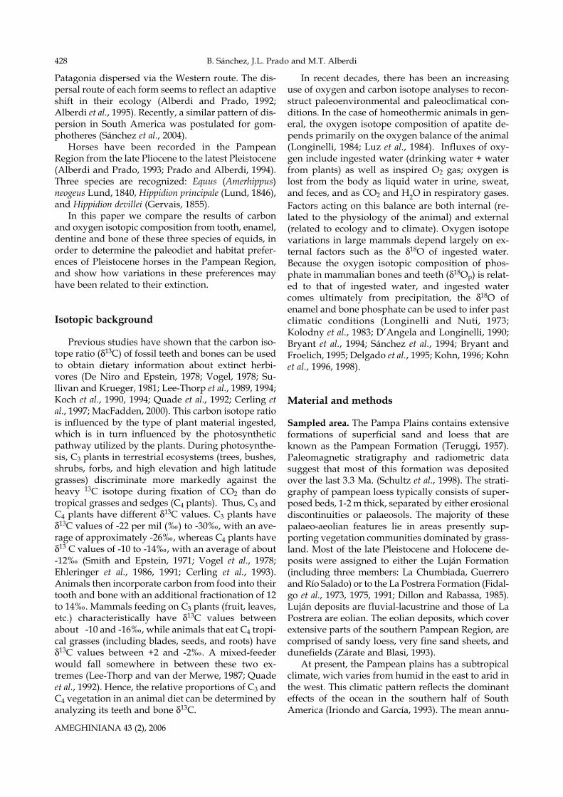
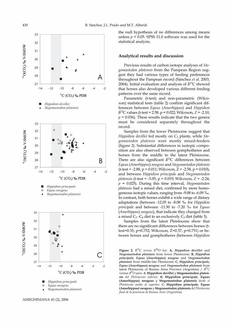
Samples from the lower Pleistocene suggest thatHippidion devillei fed mostly on C3 plants, while Ste-gomastodon platensis were mostly mixed-feeders(figure 2). Substantial differences in isotopic compo-sition are also observed between gomphotheres andhorses from the middle to the latest Pleistocene.There are also significant δ13C differences betweenEquus (Amerhippus) neogeus and Stegomastodon platensis(t-test = -2.88, p = 0.011; Wilcoxon, Z = -2.58, p = 0.010),and between Hippidion principale and Stegomastodonplatensis (t-test = -3.05, p = 0.019; Wilcoxon, Z = -2.24,p = 0.025). During this time interval, Stegomastodonplatensis had a mixed diet, confirmed by more homo-geneous isotopic values, ranging from -9.08 to -6.09 ‰.In contrast, both horses exhibit a wide range of dietaryadaptations (between -12.05 to -8.08 ‰ for Hippidionprincipale and between -11.50 to -7.20 ‰ for Equus(Amerhippus) neogeus), that indicate they changed froma mixed C3 -C4 diet to an exclusively C3 diet (table 3).

Samples from the latest Pleistocene show thatthere are no significant differences between horses (t-test=0.35, p=0.752; Wilcoxon, Z=0.37, p=0.751) or be-tween horses and gomphotheres (between Hippidion


Figure 2. δ13C versus δ18O for: A, Hippidion devillei andStegomastodon platensis from lower Pleistocene; B, Hippidionprincipale, Equus (Amerhippus) neogeus and Stegomastodonplatensis from middle-late Pleistocene; C, Hippidion principale,Equus (Amerhippus) neogeus and Stegomastodon platensis fromlatest Pleistocene of Buenos Aires Province (Argentina) / δ13Cversus δ18O para: A, Hippidion devillei y Stegomastodon platen-sis del Pleistoceno inferior; B, Hippidion principale, Equus(Amerhippus) neogeus y Stegomastodon platensis desde elPleistoceno medio al superior; C, Hippidion principale, Equus(Amerhippus) neogeus y Stegomastodon platensis del Pleistocenofinal de la provincia de Buenos Aires (Argentina).


principale and Stegomastodon platensis (t-test = -2.61, p= 0.80; Wilcoxon, Z=-1.83, p = 0.068; and betweenEquus (Amerhippus) neogeus and Stegomastodon platen-

sis (t-test =-0.82, p = 0.437; Wilcoxon, Z=-0.84, p=0.401). These results indicate that the three specieswere mostly C3 grazers.


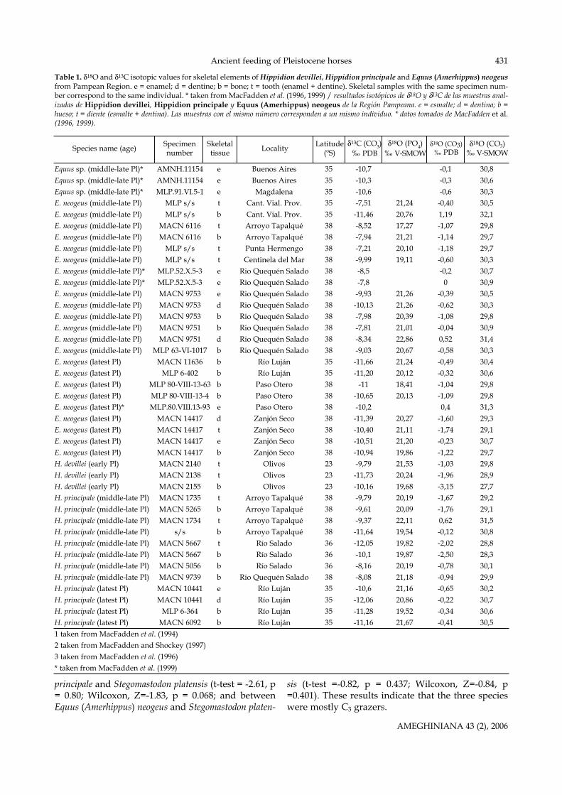
Table 1. δ18O and δ13C isotopic values for skeletal elements of Hippidion devillei, Hippidion principale and Equus (Amerhippus) neogeusfrom Pampean Region. e = enamel; d = dentine; b = bone; t = tooth (enamel + dentine). Skeletal samples with the same specimen num-ber correspond to the same individual. * taken from MacFadden et al. (1996, 1999) / resultados isotópicos de δ18O y δ13C de las muestras anal-izadas de Hippidion devillei, Hippidion principale y Equus (Amerhippus) neogeus de la Región Pampeana. e = esmalte; d = dentina; b =hueso; t = diente (esmalte + dentina). Las muestras con el mismo número corresponden a un mismo individuo. * datos tomados de MacFadden et al.(1996, 1999).

Species name (age) Specimen number

Skeletaltissue Locality Latitude

(ºS)δ13C (CO3)

‰ PDBδ18O (PO4)

‰ V-SMOWδ18O (CO3)

‰ PDBδ18O (CO3)

‰ V-SMOW

Equus sp. (middle-late Pl)* AMNH.11154 e Buenos Aires 35 -10,7 -0,1 30,8Equus sp. (middle-late Pl)* AMNH.11154 e Buenos Aires 35 -10,3 -0,3 30,6Equus sp. (middle-late Pl)* MLP.91.VI.5-1 e Magdalena 35 -10,6 -0,6 30,3E. neogeus (middle-late Pl) MLP s/s t Cant. Vial. Prov. 35 -7,51 21,24 -0,40 30,5E. neogeus (middle-late Pl) MLP s/s b Cant. Vial. Prov. 35 -11,46 20,76 1,19 32,1E. neogeus (middle-late Pl) MACN 6116 t Arroyo Tapalqué 38 -8,52 17,27 -1,07 29,8E. neogeus (middle-late Pl) MACN 6116 b Arroyo Tapalqué 38 -7,94 21,21 -1,14 29,7E. neogeus (middle-late Pl) MLP s/s t Punta Hermengo 38 -7,21 20,10 -1,18 29,7E. neogeus (middle-late Pl) MLP s/s t Centinela del Mar 38 -9,99 19,11 -0,60 30,3E. neogeus (middle-late Pl)* MLP.52.X.5-3 e Rio Quequén Salado 38 -8,5 -0,2 30,7E. neogeus (middle-late Pl)* MLP.52.X.5-3 e Rio Quequén Salado 38 -7,8 0 30,9E. neogeus (middle-late Pl) MACN 9753 e Rio Quequén Salado 38 -9,93 21,26 -0,39 30,5E. neogeus (middle-late Pl) MACN 9753 d Rio Quequén Salado 38 -10,13 21,26 -0,62 30,3E. neogeus (middle-late Pl) MACN 9753 b Rio Quequén Salado 38 -7,98 20,39 -1,08 29,8E. neogeus (middle-late Pl) MACN 9751 b Rio Quequén Salado 38 -7,81 21,01 -0,04 30,9E. neogeus (middle-late Pl) MACN 9751 d Rio Quequén Salado 38 -8,34 22,86 0,52 31,4E. neogeus (middle-late Pl) MLP 63-VI-1017 b Rio Quequén Salado 38 -9,03 20,67 -0,58 30,3E. neogeus (latest Pl) MACN 11636 b Río Luján 35 -11,66 21,24 -0,49 30,4E. neogeus (latest Pl) MLP 6-402 b Río Luján 35 -11,20 20,12 -0,32 30,6E. neogeus (latest Pl) MLP 80-VIII-13-63 b Paso Otero 38 -11 18,41 -1,04 29,8E. neogeus (latest Pl) MLP 80-VIII-13-4 b Paso Otero 38 -10,65 20,13 -1,09 29,8E. neogeus (latest Pl)* MLP.80.VIII.13-93 e Paso Otero 38 -10,2 0,4 31,3E. neogeus (latest Pl) MACN 14417 d Zanjón Seco 38 -11,39 20,27 -1,60 29,3E. neogeus (latest Pl) MACN 14417 t Zanjón Seco 38 -10,40 21,11 -1,74 29,1E. neogeus (latest Pl) MACN 14417 e Zanjón Seco 38 -10,51 21,20 -0,23 30,7E. neogeus (latest Pl) MACN 14417 b Zanjón Seco 38 -10,94 19,86 -1,22 29,7H. devillei (early Pl) MACN 2140 t Olivos 23 -9,79 21,53 -1,03 29,8H. devillei (early Pl) MACN 2138 t Olivos 23 -11,73 20,24 -1,96 28,9H. devillei (early Pl) MACN 2155 b Olivos 23 -10,16 19,68 -3,15 27,7H. principale (middle-late Pl) MACN 1735 t Arroyo Tapalqué 38 -9,79 20,19 -1,67 29,2H. principale (middle-late Pl) MACN 5265 b Arroyo Tapalqué 38 -9,61 20,09 -1,76 29,1H. principale (middle-late Pl) MACN 1734 t Arroyo Tapalqué 38 -9,37 22,11 0,62 31,5H. principale (middle-late Pl) s/s b Arroyo Tapalqué 38 -11,64 19,54 -0,12 30,8H. principale (middle-late Pl) MACN 5667 t Río Salado 36 -12,05 19,82 -2,02 28,8H. principale (middle-late Pl) MACN 5667 b Río Salado 36 -10,1 19,87 -2,50 28,3H. principale (middle-late Pl) MACN 5056 b Río Salado 36 -8,16 20,19 -0,78 30,1H. principale (middle-late Pl) MACN 9739 b Rio Quequén Salado 38 -8,08 21,18 -0,94 29,9H. principale (latest Pl) MACN 10441 e Río Luján 35 -10,6 21,16 -0,65 30,2H. principale (latest Pl) MACN 10441 d Río Luján 35 -12,06 20,86 -0,22 30,7H. principale (latest Pl) MLP 6-364 b Río Luján 35 -11,28 19,52 -0,34 30,6H. principale (latest Pl) MACN 6092 b Río Luján 35 -11,16 21,67 -0,41 30,51 taken from MacFadden et al. (1994)2 taken from MacFadden and Shockey (1997)3 taken from MacFadden et al. (1996)* taken from MacFadden et al. (1999)


Mean δ18O results range between 28.8‰ and30.5‰, but there are no significant differencesamong the mean δ18O values for the stratigraphicalintervals considered. The overall range of the totalmean isotopic values for equids is approximately1.7‰. Based on the equation for living horses (Delga-do et al., 1995), the isotopic values indicate a totalrange of the environmental water isotopic composi-tion is this area to be approximately 2.9‰. If wetranslate the data into temperatures, bearing in mindthat the Dansgaard equation is calculated for north-ern Europe (Dansgaard, 1964), we obtain approxi-mate temperature values and are able to comparethem with current temperatures. So, the range ofδ18O (H2O) calculated for the equids of the PampeanRegion would correspond to a variation of 4.2ºC inannual mean temperatures from early to latestPleistocene. For example, current annual mean tem-perature range from 13.4º in Mar del Plata city (38º S),16.4ºC for Buenos Aires city (34ºS), to 19.2ºC in SantaFé city (32ºS). Our results indicate that the interval ofmean temperature variation inferred for thePleistocene is in the same order of variation as cur-rent temperature variation (at 6º of latitude). Sánchezand Alberdi (1996) report similar results for pam-pean gomphotheres.

Our results indicate that a relationship exists be-tween the extinction of large mammals and their di-etary preferences. Currently, Quaternary extinction

of large mammals is explained by two main groupsof accepted theories. One group of theories attributeslarge mammal extinction to climatic and ecologicalchanges, while the other group holds man’s huntingactivities responsible.

The most widely accepted hypothesis related toclimatic and ecological factors postulates that nutri-tional stress induced by rapid changes in plant com-munities may have been a primary cause of extinc-tion (Graham and Lundelius, 1984; King andSaunders, 1984). This model implies that large mam-mals died off because they were specialized feeders,adapted to certain kinds of plants that may have dis-appeared during the Holocene. With this in mind,Guthrie (1984) hypothesized that plant diversity wasgreater, and the growing season longer, in thePleistocene than in the Holocene. These changes inplant diversity and growing season may have affect-ed the large mammal populations that were special-ist feeders. In addition, Vrba (1993) suggests that her-bivores might be more vulnerable to changes in cli-mate that affect vegetation structure, while omni-vores would be less affected as they are more able toadapt to different types of food and habitats.

The Pleistocene was characterized by rapid andrepeated climatic fluctuations that caused the forma-tion and retreat of massive continental glaciers insouthern South America. The fact that large mammalextinctions in this region occurred at the same time as


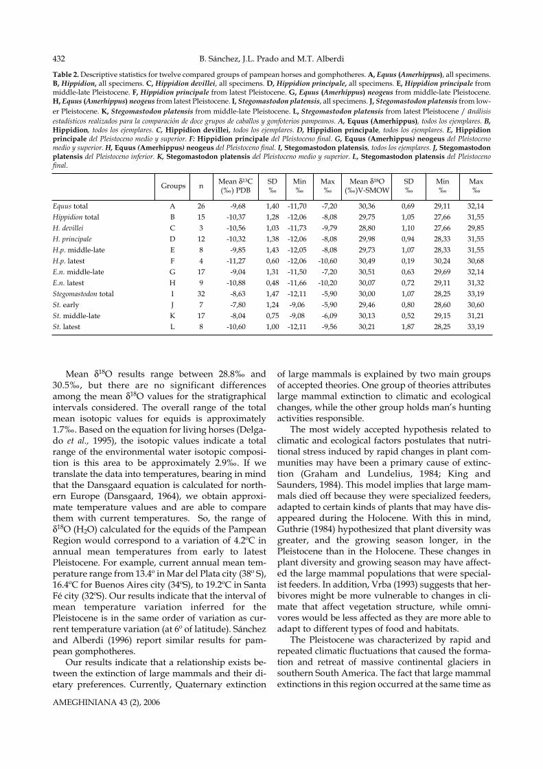
Table 2. Descriptive statistics for twelve compared groups of pampean horses and gomphotheres. A, Equus (Amerhippus), all specimens.B, Hippidion, all specimens. C, Hippidion devillei, all specimens. D, Hippidion principale, all specimens. E, Hippidion principale frommiddle-late Pleistocene. F, Hippidion principale from latest Pleistocene. G, Equus (Amerhippus) neogeus from middle-late Pleistocene.H, Equus (Amerhippus) neogeus from latest Pleistocene. I, Stegomastodon platensis, all specimens. J, Stegomastodon platensis from low-er Pleistocene. K, Stegomastodon platensis from middle-late Pleistocene. L, Stegomastodon platensis from latest Pleistocene / análisisestadísticos realizados para la comparación de doce grupos de caballos y gonfoterios pampeanos. A, Equus (Amerhippus), todos los ejemplares. B,Hippidion, todos los ejemplares. C, Hippidion devillei, todos los ejemplares. D, Hippidion principale, todos los ejemplares. E, Hippidionprincipale del Pleistoceno medio y superior. F: Hippidion principale del Pleistoceno final. G, Equus (Amerhippus) neogeus del Pleistocenomedio y superior. H, Equus (Amerhippus) neogeus del Pleistoceno final. I, Stegomastodon platensis, todos los ejemplares. J, Stegomastodonplatensis del Pleistoceno inferior. K, Stegomastodon platensis del Pleistoceno medio y superior. L, Stegomastodon platensis del Pleistocenofinal.

Equus total A 26 -9,68 1,40 -11,70 -7,20 30,36 0,69 29,11 32,14Hippidion total B 15 -10,37 1,28 -12,06 -8,08 29,75 1,05 27,66 31,55H. devillei C 3 -10,56 1,03 -11,73 -9,79 28,80 1,10 27,66 29,85H. principale D 12 -10,32 1,38 -12,06 -8,08 29,98 0,94 28,33 31,55H.p. middle-late E 8 -9,85 1,43 -12,05 -8,08 29,73 1,07 28,33 31,55H.p. latest F 4 -11,27 0,60 -12,06 -10,60 30,49 0,19 30,24 30,68E.n. middle-late G 17 -9,04 1,31 -11,50 -7,20 30,51 0,63 29,69 32,14E.n. latest H 9 -10,88 0,48 -11,66 -10,20 30,07 0,72 29,11 31,32Stegomastodon total I 32 -8,63 1,47 -12,11 -5,90 30,00 1,07 28,25 33,19St. early J 7 -7,80 1,24 -9,06 -5,90 29,46 0,80 28,60 30,60St. middle-late K 17 -8,04 0,75 -9,08 -6,09 30,13 0,52 29,15 31,21St. latest L 8 -10,60 1,00 -12,11 -9,56 30,21 1,87 28,25 33,19

Groups n Mean δ13C (‰) PDB

SD‰

Min‰

Max‰

Mean δ18O(‰)V-SMOW

SD‰

Min‰

Max‰


the major climatic deterioration associated with thelast glacial cycle, has prompted considerable specu-lation about the extent to which these events arecausally related (Borrero, 1984; Politis and Prado,1990). During the latest Pleistocene to earliestHolocene in the Pampean Region, all megamammals(over 1 t) and a majority of large mammals (over 44kg) suffered massive extinctions. Recent studies(Lessa and Fariñas, 1996; Lessa et al., 1997) based onlate mammals from America, corroborate the ideathat large body mass is the only factor strongly asso-ciated with the probability of extinction. Based onlate mammals from the Pampean Region, Prado et al.(2001a, 2001b) analyzed the quantitative relationshipbetween climatic changes and mammal diversity,and corroborated the vulnerability of large mammalsto extinction.

The second group of theories hypothesises that

large mammal extinction was a direct result of manand his hunting activities. Among this group, Politisand Gutiérrez (1998) identified three main models:the first postulated by Martin (1967, 1973, 1984), pro-posed that the extinction of large mammals fromNorth America, South America and Australia was re-lated to sudden human expansion into these conti-nents. This “overkill” hypothesis is supported by thesynchronism of extinction with the arrival of largenumbers of humans to these continents and by math-ematical simulation (Alroy, 2001). Recently, Cione etal. (2003) suggested that the main cause of the extinc-tion in South America was due to human overhunt-ing but was also influenced by climatic changes andreduction of open areas. Large mammals were adapt-ed to the dry and cold climate and open areas thatpredominated in South America during Pleistocene.The periodic interglacial increases in temperatureand humidity may have provoked shrinking of openareas and reduction of the biomass of mammalsadapted to these habitats. The authors refer to this al-ternation of low and high biomass of animals fromopened and closed areas as the “Broken Zig-Zag”.

The archaeological record from the PampeanRegion shows that Pleistocene mammals were com-mon in Paleo-Indian sites (Miotti and Salemme,1999). There are several archaeological sites whereextinct mammals were recorded: La Moderna, CerroLa China 1, Zanjon Seco 2, Laguna Tres Reyes, Cam-po Laborde, Arroyo Seco 2 and Paso Otero 5. Each ofthese sites has special characteristics and differentkinds of associations. In particular, the last two sitescontain horse remains. Among the nine extinctspecies found in Arroyo Seco 2, only horses[Hippidion and Equus (Amerhippus)] and the giantsloth (Megatherium) are numerically significant(Politis et al., 1987, 1995). For the early component ofthis site, three radiocarbon dates were obtained onEquus (Amerhippus) neogeus (AA-7964, with AMS11250±105 yrs BP; OXA-4590, with AMS 11000 ± 100yrs BP and TO-1504, with AMS 8890±90 yrs BP).Tonni et al. (2003) also present radiocarbon data onEquus (Amerhippus) neogeus from Quequén Grande(the upper part of Guerrero member, LujánFormation) with values of 10290±130 yrs BP (LP-1235). In addition, the datum of 8890 yrs BP providesexact chronological information with regard to thelatest record, or taxon-data (Grayson, 1987) of Equus(Amerhippus) neogeus.

The influence of early hunter-gatherers on horsesis difficult to quantify. Not enough information isavailable to evaluate the extent to which the pressurecaused by hunting affected the late populations ofthese species. There is evidence that verifies that hu-mans were present in the Pampean Region around11,500 yrs B P and that they coexisted with the extinct


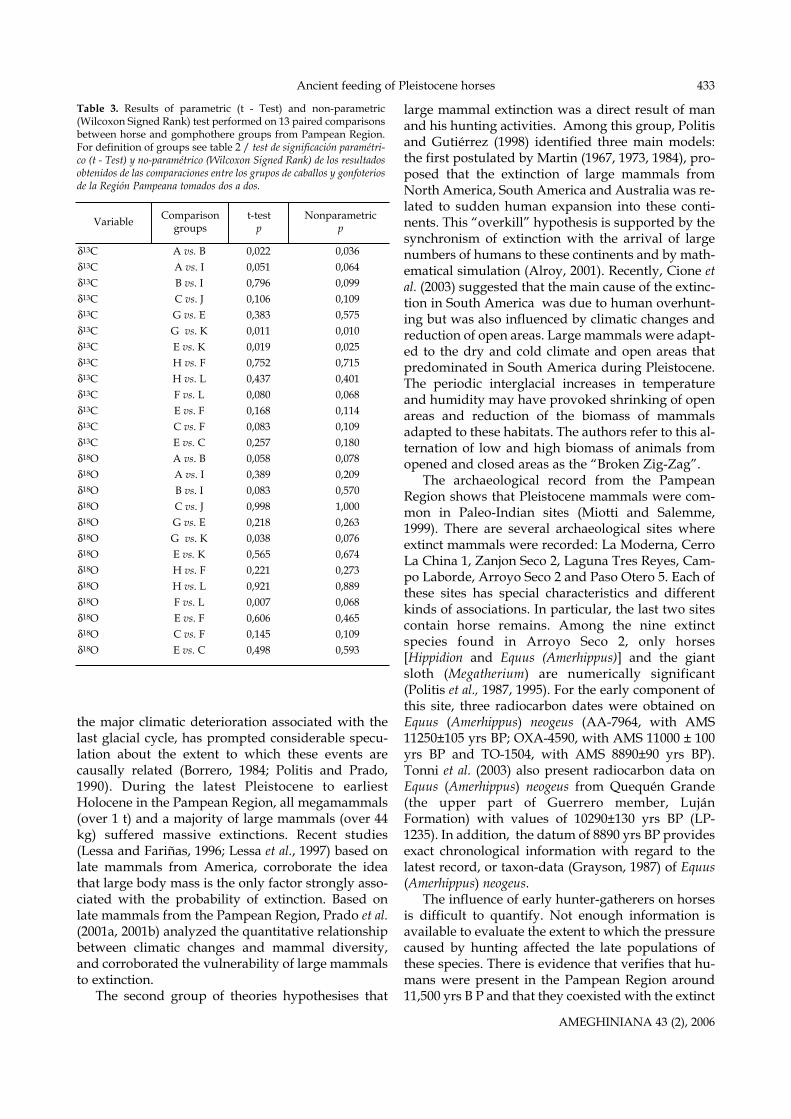
δ13C A vs. B 0,022 0,036δ13C A vs. I 0,051 0,064δ13C B vs. I 0,796 0,099δ13C C vs. J 0,106 0,109δ13C G vs. E 0,383 0,575δ13C G vs. K 0,011 0,010δ13C E vs. K 0,019 0,025δ13C H vs. F 0,752 0,715δ13C H vs. L 0,437 0,401δ13C F vs. L 0,080 0,068δ13C E vs. F 0,168 0,114δ13C C vs. F 0,083 0,109δ13C E vs. C 0,257 0,180δ18O A vs. B 0,058 0,078δ18O A vs. I 0,389 0,209δ18O B vs. I 0,083 0,570δ18O C vs. J 0,998 1,000δ18O G vs. E 0,218 0,263δ18O G vs. K 0,038 0,076δ18O E vs. K 0,565 0,674δ18O H vs. F 0,221 0,273δ18O H vs. L 0,921 0,889δ18O F vs. L 0,007 0,068δ18O E vs. F 0,606 0,465δ18O C vs. F 0,145 0,109δ18O E vs. C 0,498 0,593

Variable Comparisongroups

t-testp

Nonparametricp

Table 3. Results of parametric (t - Test) and non-parametric(Wilcoxon Signed Rank) test performed on 13 paired comparisonsbetween horse and gomphothere groups from Pampean Region.For definition of groups see table 2 / test de significación paramétri-co (t - Test) y no-paramétrico (Wilcoxon Signed Rank) de los resultadosobtenidos de las comparaciones entre los grupos de caballos y gonfoteriosde la Región Pampeana tomados dos a dos.


large mammals for three thousand years or more.Politis et al. (1995) suggest that humans played a sec-ondary role in the extinction of the native SouthAmerican fauna, but had a greater effect on immi-grant fauna such as horses and mastodons. Miottiand Salemme (1999) were able to verify evidence ofthe consumption of horses by the cut marks theyfound in fossil bone.

It has been difficult for proponents of the climatichypothesis to isolate a single climatic cause for theextinctions. Climate may have provoked changes inflora communities and as consequence altered herbi-vores diets and caused heightened periods of compe-tition (Graham and Lundelius, 1984). Also, a shor-tened growing season at the end of the Pleistocenewould have created environmental stress for largemammals (Guthrie, 1984). Although horses mayhave been able to adapt to any one of these environ-mental perturbations, the combination of all of themat the same time may have been devastating forspecies that showed more selective dietary adapta-tions. Undoubtedly, pressures exerted by hunter-gatherers may have also added to the environmentalstresses.

Conclusion

The objective of this study was to reconstruct theancient diet and habitat preference of Hippidion devi-llei, Hippidion principale and Equus (Amerhippus) neo-geus from the Pampean Region using carbon andoxygen isotopic composition of teeth and bones.Carbon isotope analyses reveal that these horses haddifferent food adaptations. Due to their high crow-ned teeth, it has traditionally been thought that hors-es fed on abrasive grasses. However, carbon isotopicdata from the Pampean Region indicate that thesehorses ranged from mixed feeders to more special-ized C3 grazers. Hippidion devillei from lower Pleisto-cene were principally C3 grazers. Specimens of Hippi-dion principale and Equus (Amerhippus) neogeus fromthe middle Pleistocene had a C3 to mixed C3-C4 diet,while specimens from latest Pleistocene were pri-marily C3 grazers. These results are partially corrob-orated by data from the lower to middle Pleistocenefrom Bolivia (MacFadden and Shockey, 1997; Mac-Fadden, 2000). These authors indicate that horsesfrom Tarija ranged from largely C4 grazers (Equus in-sulatus) to principally mixed-feeders (Hippidion prin-cipale and Hippidion devillei ) which suggests that theymay have partitioned their available food resourcesacross a broad spectrum of pastures.

We believe that horses from middle Pleistoceneexhibited opportunistic feeding strategies and con-sequently may have been adapted to diverse habi-

tats, even though the majority of equids from themiddle Pleistocene showed a preference for mixed-feeding. In contrast, populations from late Pleis-tocene appear to have adapted to a more selectivediet, which restricted their habitat preference. Asimilar isotopic pattern was found for Stegomastodonplatensis from the Pampean Region (Sánchez et al.,2003). The authors propose that gomphotheres weredriven to extinction because they were specializedfeeders, adapted to a kind of plant that may havedisappeared during the Holocene (Sánchez et al.,2004).

Several nutritional hypotheses postulated for la-test Pleistocene megamammal extinctions operateunder the assumption that extinct taxa had special-ized diets. The resource partitioning preference ofHippidion principale and Equus (Amerhippus) neogeusfrom latest Pleistocene in Pampean Region supportsthese hypotheses.

Acknowledgements

We wish to thank the curators of the Museo de La Plata(Argentina), and Museo Argentino de Ciencias Naturales“Bernardino Rivadavia” of Buenos Aires, who were in charge ofthe remains. The manuscript was greatly improved by thoughtfulreview from Gustavo Martínez and Gustavo Politis, and also byMartín Ubilla and an anonymous reviewer. Mr. James Watkins re-vised the English text. Samples were analyzed in the IsotopeGeochemistry Laboratory at the Università di Trieste, and Serviciode Isótopos Estables of the Universidad Autónoma de Madrid (SI-DI). This work was supported by a joint Research Project from theAgencia Española de Cooperación Iberoamericana, Spain -Argentina (2000-2001) and CSIC 2002; Projects PB94-0071, PB97-1250, and BTE2001-1864 from the Dirección General deInvestigación Científica y Técnica of Spain; grants from theUniversidad Nacional del Centro, and the CONICET Project PIP-2000-02773, Argentina.

References

Alberdi, M.T. and Prado, J.L. 1992. El registro de Hippidion Owen,1869 y Equus (Amerhippus) Hoffstetter, 1950 (Mammalia,Perissodactyla) en América del Sur. Ameghiniana 29: 265-284.

Alberdi, M.T. and Prado, J.L. 1993. Review of the genus HippidionOwen, 1869 (Mammalia; Perissodactyla) from the Pleistoceneof South America. Zoological Journal of the Linnean Society 108:1-22.

Alberdi, M.T., Prado, J.L. and Ortiz Jaureguizar, E. 1995. Patternsof body size changes in fossil and living Equini (Peri-ssodactyla). Biological Journal of the Linnean Society 54: 349-370.

Alroy, J. 2001. A Multispecies Overkill Simulation of the End-Pleistocene Megafaunal Mass Extinction. Science 292: 1893-1896.

Ameghino, F. 1888. Rápidas diagnosis de algunos mamíferos fósilesnuevos de la República Argentina. Obras Completas, BuenosAires V, pp. 469-480.

Borrero, L. 1984. Pleistocene extinctions in South America.Quaternary of South America and Antarctic Peninsula 2: 115-125.

Bryant, J.D. and Froelich, P.N. 1995. A model of oxygen isotope



fractionation in body water of large mammals. Geochimica etCosmochimica Acta 59: 4523-4537.

Bryant, J.D., Luz, B. and Froelich, P.N. 1994. Oxygen isotopic com-position of fossil horse tooth phosphate as a record of conti-nental paleoclimate. Palaeogeography, Palaeoclimatology,Palaeoecology 107: 303-316.

Cerling, T.E., Wang, Y., and Quade, J. 1993. Expansion of C4ecosystems as an indicator of global ecological change in theLate Miocene. Nature 361: 344-45.

Cerling, T.E., Harris, J.M., MacFadden, B.J., Leakey, M.G., Quade,J., Eisenmann, V., and Ehleringer, J.R. 1997. Global vegetationchange through the Miocene/Pliocene boundary. Nature 389:153-158.

Cione, L.A. and Tonni, E.P. 1995. Chronostratigraphy and “Land-Mammal Ages” in the Cenozoic of Southern South America:Principles, practices, and the “Uquian” Problem. Journal ofPaleontology 69: 135-159.

Cione, L.A. and Tonni, E.P. 1999. Biostratigraphy and chronolog-ical scale of upper-most Cenozoic in the Pampean Area,Argentina. Quaternary of South America and AntarcticaPeninsula 12: 23-51.

Cione, A.L., Tonni, E.P. and Soibelzon, L. 2003. The Broken Zig-Zag: Late Cenozoic large mammal and tortoise extinction inSouth America. Revista del Museo Argentino de CienciasNaturales 5: 1-19.

D’Angela, D. and Longinelli, A. 1990. Oxygen isotopic composi-tion of fossil mammal bones of Holocene age: paleoclimato-logical considerations. Chemical Geology (Isotopic GeoscienceSection) 103: 171-179.

Dansgaard, W. 1964. Stable isotopes in precipitation. Tellus 16(4):436-468.

Delgado, A., Iacumin, P., Stenni, B., Sanchez, B., and Longinelli,A. 1995. Oxygen isotope variations of phosphate in mam-malian bone and tooth enamel. Geochimica et CosmochimicaActa 59: 4299-4305.

De Niro, M. J. and Epstein, J. 1978. Influence of diet on the distri-bution of carbon isotopes in animals. Geochima et CosmochimicaActa 42: 495-506.

Dillon, C.A. and Rabassa, J. 1985. Miembro La Chumbiada,Formación Luján (Pleistoceno, provincia de Buenos Aires):Una nueva unidad estratigráfica del valle del Río Salado.Primeras Jornadas Geológicas Bonaerenses, Resúmenes 27.

Ehleringer, J.R., Field, C.B., Lin, Z.F., and Kuo, C.Y. 1986. Leaf car-bon isotope and mineral composition in subtropical plantsalong an irradiance cline. Oecologia 70: 520-526.

Ehleringer, J.R., Sage, R.F., Flanagan, L.B., and Pearcy, R.W. 1991.Climatic change and evolution of C4 photosynthesis. Trends inEcology and Evolution 6: 95-99.

Fidalgo, F., De Francesco, F.O., and Colado, U. 1973. Geología su-perficial en las hojas Castelli, J.M. Cobo y Monasterio (Prov.de Buenos Aires). 5º Congreso Geológico Argentino (BuenosAires), 4: 27-39.

Fidalgo, F., De Francesco, F.O., and Pascual, R. 1975. Geología su-perficial de la llanura Bonaerense. 6º Congreso GeológicoArgentino (Bahía Blanca), Relatorio: 100-138.

Fidalgo, F., Riggi, J.C., Correa, H. and Porro, N. 1991. Los ‘Se-dimentos Postpampeanos’ continentales en el ámbito bonae-rense. Revista de la Asociación Geológica Argentina 47: 239-256.

Gervais, P. 1855. Recherches sur les Mammifères fossiles de l’Amériqueméridionale. P. Bertrend, Libraire-Editeur, Paris, 63 pp.

Graham, R.W., and Lundelius, E.L. 1984. Coevolutionary disequi-librium and Pleistocene Extinction. In: P.S. Martin and R.G.Klein (eds.), Quaternary Extinctions: A Prehistoric Revolution.University of Arizona Press, Tucson, pp. 223-249.

Grayson, D.K. 1987. An analysis of the Chronology of LatePleistocene Mammalian Extinctions in North America.Quaternary Research 28: 281-289.

Guthrie, R.D. 1984. Mosaics, Allelochemics and Nutrients. AnEcological Theory of Late Pleistocene Megafaunal extinction.In: P.S. Martin and R.G. Klein (eds.), Quaternary Extinctions: A

Prehistoric Revolution. University of Arizona Press, Tucson, pp.259-298.

Iriondo, M.H. and García, N.O. 1993. Climatic variations in theArgentine plains during the last 18,000 years. Palaeogeography,Palaeoclimatology, Palaeoecology 101: 209-220.

King, J. E. and Saunders, J. J. 1984. Environmental insularity andthe extinction of the American mastodont. In: P.S. Martin andR.G. Klein (eds.), Quaternary Extinctions: A PrehistoricRevolution. University of Arizona Press, Tucson, pp. 315-339.

Koch, P.L., Fisher, D.C., and Dettman, D. 1989. Oxygen isotopevariation in the tusks of extinct proboscideans: a measure ofseason of death and seasonality. Geology 17: 515-519.

Koch, P.L., Behrensmeyer, A.K., Tuross, N. and Fogel, M.L. 1990.The fidelity of isotopic preservation during bone weatheringand burial. Annual Report of the Director Geophysical Laboratory,Carnegie Institution of Washington 1989-1990: 105-110.

Koch, P.L., Fogel, M.L. and Tuross, N. 1994. Tracing the diets offossil animals using stable isotopes. In: K. Lajtha and R.H.Michener (eds.), Stable isotopes in Ecology and environmentalScience. Blackwell Scientific, pp. 63-92

Koch, P.L., Tuross, N., and Fogel, M.L. 1997. The effects of sampletreatment and diagenesis on the isotopic integrity of carbon inbiogenic hydroxylapatite. Journal of Archaeological Science 24:417-429.

Kohn, M.J. 1996. Predicting animal ?18O: accounting for diet andphysiological adaptation. Geochimica et Cosmochimica, Acta 60:4811-4829.

Kohn, M.J., Schoeninger, M.J., and Valley, J.W. 1996. Herbivoretooth oxygen isotope compositions: effects of diet and physi-ology. Geochimica et Cosmochimica, Acta 60: 3889-3896.

Kohn, M.J., Schoeninger, M.J., and Valley, J.W. 1998. Variability inoxygen isotope compositions of herbivore teeth: reflections ofseasonality or developmental physiology? Chemical Geology152: 97-112.

Kolodny, Y., Luz, B. and Navon, O. 1983. Oxygen isotope varia-tions in phosphate of biogenic apatites, I. Fish bone apatite.Rechecking the rules of the game. Earth and Planetary ScienceLetters 64: 398-404.

Lee-Thorp, J.A. and van der Merwe, N.J. 1987. Carbon isotopeanalysis of fossil bones apatite. South African Journal of Science83: 712-715.

Lee-Thorp, J.A., van der Merwe, N.J., and Brain, C.K. 1989.Isotopic evidence for dietary differences between two extinctbaboon species from Swartkrans. Journal of Human Evolution18: 183-190.

Lee-Thorp, J.A., van der Merwe, N.J., and Brain, C.K. 1994. Diet ofAustralopithecus robustus at Swartkrans from stable carbon iso-topic analysis. Journal of Human Evolution 27: 361-372.

Lessa, E.P., and Fariñas, R.A. 1996. Reassessment of extinctionpatterns among the Late Pleistocene mammals of SouthAmerica. Palaeontology 39: 651-662.

Lessa, E.P., Valkenburgh, B.van and Fariñas, R.A. 1997. Testinghypotheses of differential mammalian extinctions subsequentto the Great American Biotic Interchange. Palaeogeography,Palaeoclimatology, Palaeoecology 135: 157-162.

Longinelli, A. 1984. Oxygen isotopes in mammal bone phosphate:a new tool for paleohydrological and paleoclimatological re-search? Geochimica et Cosmochimica, Acta 48: 385-390.

Longinelli, A. and Nuti, S. 1973. Oxygen isotope measurements ofphosphate from fish teeth and bones. Earth and PlanetaryScience Letters 20: 337-340.

Lund, P.W. 1840. Blik paa Brasiliens Dyreverden for SidsteJordomvaeltning. Tredie Afhandling: Forsaettelse af Patte-dyrene. Det Kongelige Danske Videnskabernes Selskbas Na-turvidenskabelige og Mathematiske Afhandlinger 8: 217-272.

Lund, P.W. 1846. Meddlelse af det Udbytte de I 1844 undersögteKnoglehuler Have avgivet til hundskaben om BrasiliensDyreverden för sidste Jordomvaeltning. Det köngelige DanskeVidenskabernes Selskabs naturvidenskabelige og mathematiskAfhandlinger 12, 57-94.



Luz, B., Kolodny, Y. and Horowitz, M. 1984. Fractionation of oxy-gen isotopes between mammalian bone-phosphate and envi-ronmental drinking water. Geochimica et Cosmochimica, Acta 48:1689-1693.

MacFadden, B.J. 2000. Middle Pleistocene climate change record-ed in fossil mammal teeth from Tarija, Bolivia, and upper lim-it of the Ensenadan Land-Mammal Age. Quaternary Research54: 121-131.

MacFadden, B.J., Cerling, T.E., Harris, J.M., and Prado, J.L. 1999.Ancient latitudinal gradients of C3/C4 grasses interpretedfrom stable isotopes of New World Pleistocene horses. GlobalEcology and Biogeography 8: 137-149.

MacFadden, B.J., Cerling, T.E. and Prado, J. L. 1996. CenozoicTerrestrial Ecosystem in Argentina Evidence from Carbon iso-topes of Fossil Mammal Teeth. Palaios 11: 319-327.

MacFadden, B.J., and Shockey, B.J. 1997. Ancient feeding ecologyand niche differentiation of Pleistocene mammalian herbi-vores from Tarija, Bolivia: morphological and isotopic evi-dence. Paleobiology 23: 77-100.

Martin, P.S. 1967. Prehistoric Overkill. In: P.S. Martin and H.E.Wright Jr. (eds.), Pleistocene Extinction. The Search for a Cause.Yale University Press, New Haven. pp. 75-120.

Martin, P.S. 1973. The discovery of America. Science 179: 969-974.Martin, P.S. 1984. Prehistoric Overkill: The Global Model. In: P.S.

Martin and R.G. Klein (eds.), Quaternary Extinctions: APrehistoric Revolution. University of Arizona Press, Tucson. pp.354-403.

Miotti, L. and Salemme, M. 1999. Biodiversity, taxonomic richnessand specialists-generalists during Late Pleistocene/EarlyHolocene times in Pampa and Patagonia (Argentina, SouthernSouth America). Quaternary International 53/54: 53-68.

Politis, G. and Gutiérrez, M. 1998. Gliptodontes y cazadores-recolectores de la Región Pampeana (Argentina). Latin Ame-rican Antiquity 9: 111-134.

Politis G.G. and Prado, J.L. 1990. La influencia del hombre en lasextinciones faunísticas del Pleistoceno/Holoceno enAmérica: el caso pampeano. Memorias del Simposio deArqueología y Antropología Física del 5º Congreso Nacional deAntropología, Memoria de Eventos Científicos ICFES(Colombia): 31-63 pp.

Politis, G., Tonni, E.P., Fidalgo, F., Salemme, M. and Guzmán, L.1987. Man and Pleistocene Megamammals in the ArgentinePampa: Site 2 at Arroyo Seco. Current Research in the Pleistocene4: 159-161.

Politis, G.G., Prado, J.L. and Beukens, R.P. 1995. The HumanImpact In Pleistocene-Holocene Extinctions. In: E. Johnson(ed.), South America-The Pampean Case. Ancient Peoples andLandscapes. Museum of Texas Tech University, Texas. pp. 187-205.

Prado, J.L. and Alberdi, M.T. 1994. A quantitative review of thehorse Equus from South America. Palaeontology 37: 459-481.

Prado, J.L., Alberdi, M.T., Azanza, B. and Sánchez, B. 2001a.Climate and changes in mammal diversity during the latePleistocene-Holocene in the Pampean Region (Argentina).Acta Palaeontologica Polonica 46: 261-276.

Prado, J.L., Azanza, B., Alberdi, M.T. and Gómez, G. 2001b.Mammal community and Global Change during the LatePleistocene-Holocene in the Pampean Region (Argentina). In:D. Büchner (ed.), Studia honoraria: Studien in Memorian WilhelmSchüle 11: 362-375.

Quade, J., Cerling, T.E., Barry, J.C., Morgan, M.E., Pilbeam, D.R.,Chivas, A. ., Lee-Thorp, J.A. and van der Merwe, N.J. 1992. A16-Ma record of paleodiet using carbon and oxygen isotopesin fossil teeth from Pakistan. Chemical Geology (IsotopeGeoscience Section) 94: 183-192.

Sánchez-Chillón, B. and Alberdi, M.T. 1996. Taphonomic modifi-cation of oxygen isotopic composition in some SouthAmerican Quaternary mammal remains. In: G. Meléndez, M.F. Blasco, and I. Pérez (eds.), 2º Reunión de Tafonomía yFosilización. Institución Fernando el Católico, Zaragoza, pp.353-356.

Sánchez-Chillón, B., Alberdi, M.T., Leone, G., Bonadonna, F.P.,Stenni, B. and Longinelli, A. 1994. Oxygen isotopic composi-tion of fossil equid tooth and bone phosphate: an archive ofdifficult interpretation. Palaeogeography, Palaeoclimatology,Palaeoecology 107: 317-328.

Sánchez-Chillón, B., Prado, J.L. and Alberdi, M.T. 2003. Paleodiet,ecology, and extinction of Pleistocene gomphotheres(Proboscidea) from Pampean Region (Argentina). Coloquios dePaleontología, Volumen Extraordinario 1: 617-625.

Sánchez-Chillón, B., Prado, J.L. and Alberdi, M.T. 2004. Feedingecology, dispersal, and extinction of South AmericanPleistocene gomphotheres (Gomphotheriidae, Proboscidea).Paleobiology 30: 146-161.

Schultz, P.H., Zárate, M., Hames, W., Camilión, C. and King, J.1998. A 3.3 Ma impact in Argentina and possible conse-quences. Science 282: 2061-2063.

Smith, B.N. and Epstein, S. 1971. Two categories of 13C/12C ra-tios for higher plants. Plant Physiology 47: 380-384.

Sullivan, C.H. and Krueger, H.W. 1981. Carbon isotope analysisof separate chemical phases in modern and fossil bone. Nature301: 177-178.

Teruggi, M.E. 1957. The nature and origin of Argentine loess.Journal of Sedimentary Petrology 27: 322-332.

Tonni, E.P., Huarte, R.A., Carbonari, J.E. and Figini, A.J. 2003.New radiocarbon chronology for the Guerrero Menber of theLuján Formation (Buenos Aires, Argentina): palaeoclimaticsignificance. Quaternary International 109-110: 45-48.

Vogel, J.C. 1978. Isotopic assessment of the dietary habitats of un-gulates. South African Journal of Science 74: 298-301.

Vogel, J.C., Fuls, A. and Ellis, R.P. 1978. The geographical distrib-ution of kranz grasses in South Africa. South African Journal ofScience 74: 209-215.

Vrba , E.S.1993. Turnover-pulses, the Red Queen, and related top-ics. American Journal of Science 293A: 418-452.

Webb, S.D. 1991. Ecogeography and the Great AmericanInterchange. Paleobiology 17: 266-280.

Zárate, M.A. and Blasi, A. 1993. Late Pleistocene-Holocene Eoliandeposits of the southern Buenos Aires Province, Argentina. Apreliminary model. Quaternary International 17: 15-20.

Recibido: 23 de junio de 2004.Aceptado: 1 de setiembre de 2005.


Documents

Ancient feeding, ecology and extinction of Pleistocene ...digital.csic.es/bitstream/10261/12306/1/Apa 1174.-427-436Sánchez... · During the Plio-Pleistocene, ... Animals then incorporate