Angular Distribution Models for Top-of-Atmosphere

Angular Distribution Models for Top-of-Atmosphere Radiative Flux Estimation fromthe Clouds and the Earth’s Radiant Energy System Instrument on the Terra Satellite.

Part I: Methodology

NORMAN G. LOEB AND SEIJI KATO

Center for Atmospheric Sciences, Hampton University, Hampton, Virginia

KONSTANTIN LOUKACHINE

Science Applications International Corporation, Hampton, Virginia

NATIVIDAD MANALO-SMITH

Analytical Services and Materials, Hampton, Virginia

(Manuscript received 26 May 2004, in final form 10 September 2004)

ABSTRACT

The Clouds and Earth’s Radiant Energy System (CERES) provides coincident global cloud and aerosolproperties together with reflected solar, emitted terrestrial longwave, and infrared window radiative fluxes.These data are needed to improve the understanding and modeling of the interaction between clouds,aerosols, and radiation at the top of the atmosphere, surface, and within the atmosphere. This paperdescribes the approach used to estimate top-of-atmosphere (TOA) radiative fluxes from instantaneousCERES radiance measurements on the Terra satellite. A key component involves the development ofempirical angular distribution models (ADMs) that account for the angular dependence of the earth’sradiation field at the TOA. The CERES Terra ADMs are developed using 24 months of CERES radiances,coincident cloud and aerosol retrievals from the Moderate Resolution Imaging Spectroradiometer(MODIS), and meteorological parameters from the Global Modeling and Assimilation Office (GMAO)’sGoddard Earth Observing System (GEOS) Data Assimilation System (DAS) V4.0.3 product. Scene infor-mation for the ADMs is from MODIS retrievals and GEOS DAS V4.0.3 properties over the ocean, land,desert, and snow for both clear and cloudy conditions. Because the CERES Terra ADMs are global, andfar more CERES data are available on Terra than were available from CERES on the Tropical RainfallMeasuring Mission (TRMM), the methodology used to define CERES Terra ADMs is different in manyrespects from that used to develop CERES TRMM ADMs, particularly over snow/sea ice, under cloudyconditions, and for clear scenes over land and desert.

1. Introduction

One of the largest uncertainties in global climatemodels is the representation of how clouds and aerosolsinfluence the earth’s radiation budget (ERB) at the sur-face, within the atmosphere, and at the top of the at-mosphere. Because of the uncertainty in cloud–aerosol–radiation interactions, model predictions of cli-mate change vary widely from one model to the next(Cess et al. 1990, 1996; Cubasch et al. 2001). To improveour understanding of cloud–aerosol–radiation interac-tions, and to identify key areas where climate modelscan be improved, global observations are needed. The

central objective of the Clouds and the Earth’s RadiantEnergy System (CERES) mission is to provide accurateglobal cloud, aerosol, and radiation data products tofacilitate research addressing the role clouds and aero-sols play in modulating the radiative energy flow withinthe earth–atmosphere system (Wielicki et al. 1996). Thetwo CERES satellite instruments aboard the Terraspacecraft provide highly accurate shortwave (SW),longwave (LW), and infrared window (WN) radiancemeasurements and top-of-atmosphere (TOA) radiativeflux estimates globally at a 20-km spatial resolution.These data, together with coincident cloud and aerosolproperties inferred from the Moderate Resolution Im-aging Spectroradiometer (MODIS), provide a consis-tent cloud–aerosol–radiation dataset for studyingclouds and aerosols, and their influence on the ERB.

One of the challenges involved in producing ERB

Corresponding author address: Dr. Norman G. Loeb, Mail Stop420, NASA Langley Research Center, Hampton, VA 23681-2199.E-mail: [email protected]

338 J O U R N A L O F A T M O S P H E R I C A N D O C E A N I C T E C H N O L O G Y VOLUME 22

© 2005 American Meteorological Society

JTECH1712

datasets from satellites is the need to convert the radi-ance measurements at a given sun–Earth–satellite con-figuration to outgoing reflected solar and emitted ther-mal TOA radiative fluxes. To estimate TOA fluxesfrom measured CERES radiances, one must accountfor the angular dependence in the radiance field, whichis a strong function of the physical and optical charac-teristics of the scene (e.g., surface type, cloud fraction,cloud/aerosol optical depth, cloud phase, etc.), as wellas the illumination angle. Because the CERES instru-ment can rotate in azimuth as it scans in elevation, itacquires data over a wide range of angles. Conse-quently, one can construct angular distribution models(ADMs) for radiance-to-flux conversion directly fromthe CERES measurements. Furthermore, becauseCERES and MODIS are on the same spacecraft, theADMs can be derived as a function of MODIS-basedscene-type parameters that have a strong influence onradiance anisotropy.

The first set of CERES ADMs were developed using9 months of CERES and Visible Infrared Scanner(VIRS) data from the Tropical Rainfall Measuring Mis-sion (TRMM) satellite between 38°S and 38°N fromJanuary to August 1998 and March 2000 (Loeb et al.2003a). Because TRMM is in a 350-km circular precess-ing orbit with a 35° inclination angle, CERES TRMMsampled the full range of solar zenith angles over aregion every 46 days. Unfortunately, the CERESTRMM instrument suffered a voltage-converteranomaly and acquired only 9 months of scientific data.In contrast, the CERES instruments on Terra have,thus far, acquired over 4 yr of global data with coarserspatial resolution (20 km versus 10 km for CERESTRMM) from a sun-synchronous orbit at an altitude of705 km. Because of the differences in spatial resolutionand geographical coverage between the CERES instru-ments on TRMM and Terra, direct application of theCERES TRMM ADMs to CERES Terra data is inap-propriate, particularly at midlatitudes and in the polarregions.

The increased sampling that is available fromCERES Terra provides a unique opportunity to de-velop a more comprehensive set of ADMs that are suit-able for radiance-to-flux conversion with CERES Terradata and data from other broadband instruments withsimilar characteristics and orbital geometry. This paperis the first in a two-part series. Part I describes thedevelopment of new CERES Terra SW, LW, and WNADMs from 2 yr of global data. Where appropriate, wecompare the methodology used to produce CERESTerra ADMs with that used in Loeb et al. (2003a) toproduce CERES TRMM ADMs. Part II will presentextensive validation results in order to assess the accu-racy of SW, LW, and WN TOA fluxes that are derivedfrom the CERES Terra ADMs. TOA fluxes from thenew Terra ADMs will also be compared with thosefrom TRMM ADMs, as well as with fluxes based onalgorithms developed during the Earth Radiation Bud-

get Experiment (ERBE) (Smith et al. 1986; Suttles etal. 1992).

2. Observations

The Terra spacecraft, launched on 18 December1999, carries two identical CERES instruments: FlightModel (FM)-1 and -2. Terra is in a descending sun-synchronous orbit with an equator-crossing time of1030 LST. The CERES instrument is a scanning broad-band radiometer that measures filtered radiances in theSW (wavelengths between 0.3 and 5 �m), total (TOT;wavelengths between 0.3 and 200 �m), and WN (wave-lengths between 8 and 12 �m) regions. To correct forthe imperfect spectral response of the instrument, thefiltered radiances are converted to unfiltered reflectedsolar, unfiltered emitted terrestrial LW and WN radi-ances (Loeb et al. 2001). On Terra, CERES has a spa-tial resolution of approximately 20 km (equivalent di-ameter). One of the unique features of CERES is itsability to scan in either a fixed, rotating or program-mable azimuth plane scan mode. Operationally, oneCERES instrument is placed in a cross-track scan modeto optimize spatial sampling for time–space averaging(Young et al. 1998), while the second instrument is ei-ther in a rotating azimuth plane (RAP), an along-track,or a programmable azimuth plane (PAP) scan mode. Inthe RAP mode, the instrument scans in elevation as itrotates in azimuth thus acquiring radiance measure-ments from a wide range of viewing configurations. InPAP mode, CERES is programmed to collect measure-ments for a specific field campaign, for intercalibrationwith other instruments (e.g., CERES on TRMM, theGeostationary Earth Radiation Budget Instrument), orto augment sampling in specific viewing geometries(e.g., the principal plane). The nominal schedule is tooperate the second CERES instrument in along-trackmode every 15 days and in RAP mode the remainder ofthe time. In contrast, CERES TRMM was in RAPmode only every third day, and in along-track modeevery 15 days. The increase in RAP sampling forCERES Terra, together with its relatively small rangeof solar zenith angle coverage relative to CERESTRMM (which sampled all solar zenith angles every 46days), means that angular sampling at a particular solarzenith angle is increased by at least an order-of-magnitude for CERES Terra compared to CERESTRMM.

To construct ADMs for Terra, 24 months (March2000–February 2002) of the CERES Terra Edition2ASingle Scanner Footprint TOA/Surface Fluxes andClouds (SSF) product (Geier et al. 2001) are used. TheCERES SSF product combines CERES radiances andfluxes with scene information inferred from coincidentMODIS measurements (Barnes et al. 1998) and meteo-rological fields based on 4D assimilation data. Cloudproperties on the CERES Terra SSF product are in-

APRIL 2005 L O E B E T A L . 339

ferred from MODIS pixel measurements using algo-rithms that are consistent with those used to producecloud properties from VIRS (Kummerow et al. 1998)on the CERES TRMM SSF (Minnis et al. 2003). Aero-sol properties are determined from two sources—(i) byapplying the algorithm of Ignatov and Stowe (2002) and(ii) directly from the MOD04 aerosol product (Remeret al. 2005). For Terra Edition2A SSF, meteorologicalfields on the SSF are from the Global Modeling andAssimilation Office (GMAO)’s Goddard Earth Ob-serving System (GEOS) Data Assimilation System(DAS) 4.0.3 product (DAO 1996). GMAO is runningGEOS DAS V4.0.3 without any code modifications toproduce a consistent analysis over the entire CERESdata record.

As described in more detail in Loeb et al. (2003a),accurate spatial and temporal matching of imager-derived aerosol and cloud properties with CERESbroadband radiation data are obtained by accountingfor the CERES point spread function (PSF) (Smith1994) when averaging imager-derived properties overthe CERES footprint. Within a CERES footprint, theproperties of every cloudy imager pixel are assigned toa cloud layer. If there is a significant difference in cloudphase or effective pressure within a CERES field ofview (FOV), up to two nonoverlapping cloud layers aredefined. A single footprint may contain any combina-tion of a clear area and one or two distinct cloud layers(see Fig. 1 of Loeb et al. 2003a). To reduce the pro-cessing time needed to generate the CERES SSF prod-uct, the CERES team has decided to process only everyfourth MODIS pixel from every second scan line. Thisintroduces a random noise in the PSF-weighted averageimager reflectance and brightness temperature of ap-proximately 1.5% and 0.2%, respectively, over CERESFOVs (W. F. Miller 2003, personal communication).

3. CERES Terra ADM development

TOA flux is the radiant energy emitted or scatteredby the earth–atmosphere per unit area. Flux is relatedto radiance (I) as follows:

F ��o� � �0

2� �0

��2

I��o, �, �� cos� sin� d�d�, �1�

where �o is the solar zenith angle, � is the observerviewing zenith angle, and � is the relative azimuthangle defining the azimuth angle position of the ob-server relative to the solar plane. An ADM is a set ofanisotropic factors (R) for determining the TOA fluxfrom an observed radiance as follows:

F ��o� ��I��o, �, ��

R��o, �, ��. �2�

Because CERES measures the upwelling radiationfrom a scene at any given time from one or more di-rections, F (or R) cannot be measured instantaneously.

Instead, R is obtained from a set of predetermined em-pirical ADMs that are defined for several scene typeswith distinct anisotropic characteristics. For CERESTRMM, the ADMs were constructed by the sorting-into-angular-bins (SABs) method (Suttles et al. 1992;Loeb et al. 2003a). In the SAB method, a large en-semble of radiance measurements are first sorted intodiscrete angular bins and parameters that define anADM scene type, and ADM anisotropic factors for agiven scene type ( j) are given by

Rj��oi, �k, �l� ��Ij��oi, �k, �l�

Fj��oi�, �3�

where Ij is the average radiance (corrected for Earth–sun distance in the SW) in an angular bin (�oi , �k , �l),and Fj is the upwelling flux in a solar zenith angle bin�oi, which is determined by directly integrating Ij overall angles (Loeb et al. 2003a). The set of angles (�oi , �k ,�l). corresponds to the midpoint of a discrete angularbin defined by [�oi � (��o/2), �k � (��/2), �l � (��/2)],where ��o , ��, and �� represent the angular bin reso-lution. To evaluate Fj from satellite measurements,Loeb et al. (2002) showed that the reference level forthe satellite viewing geometry must be defined at least100 km above the earth’s surface in order to account forradiation contributions escaping the planet along slantpaths above the earth’s tangent point. Loeb et al. (2002)also argue that the optimal reference level for defininginstantaneous TOA fluxes in Earth radiation budgetstudies is approximately 20 km. This reference levelcorresponds to the effective radiative “top of atmo-sphere” because the radiation budget equation isequivalent to that for a solid body of a fixed diameterthat only reflects and absorbs radiation.

For CERES Terra these definitions are retained. TheSAB method is used to develop ADMs for some, butnot all, ADM scene types. As described in more detailin sections 4 and 5, where possible, we have developedADMs that are continuous functions of imager-basedretrievals, using analytical functions to represent theCERES radiance dependence on scene type. As inLoeb et al. (2003a), SW ADMs are defined explicitly asa function of three angles (�oi , �k , �l), while LW ADMsare assumed to be a function of only viewing zenithangle.

4. SW ADMs

a. Ocean

1) CLEAR

When the MODIS pixel-level cloud coverage withina CERES FOV is �0.1%, the CERES FOV is definedas being clear. Following the approach used in Loeb etal. (2003a), instantaneous TOA fluxes are determinedusing a combination of empirical and theoretical ADMsas follows:


F̂ ��I��o, �, ��

R�wk, �o, �, ��Rth�wk, I�

Rth�wk, I�� , �4�

where R(wk, �o , �, � ) is determined from wind speed–dependent empirical ADMs that are derived fromCERES data, and Rth(wk, I) and Rth(wk , I) are theo-retical radiative transfer model anisotropic factorsevaluated at the measured CERES radiance I(�o , �, � )and mean CERES radiance I(wk, �o , �, �) in a givenADM angular bin, respectively. For Terra, the angularbin resolution of the clear ocean SW ADMs has beensharpened to 2° (CERES TRMM used 10° for � and �,and 20° for � ), and the wind speed resolution has beenincreased to 2 m s1 for winds ranging from 0 to 12m s1 (the nominal wind speed intervals for CERESTRMM were �3.5, 3.5–5.5, 5.5–7.5, and �7.5 m s1).Wind speeds correspond to the 10-m level based onSpecial Sensor Microwave Imager (SSM/I) retrievals(Goodberlet et al. 1990) that have been ingested intothe GEOS-4 DAS analysis. To determine Rth(wj, I) andRth(wj , I), CERES radiances I(�o , �, �; hsfc) and I(�o , �,�; hsfc) are compared with lookup tables of theoreticalSW radiances stratified by aerosol optical depth. Here,Rth(wj, I) and Rth(wj , I) correspond to the aerosol op-

tical depth for which the theoretical radiances matchthe CERES radiances. The radiative transfer calcula-tions are from the rstar5b radiative transfer model thatis based on Nakajima and Tanaka (1986, 1988). Mari-time aerosols from Hess et al. (1998) evaluated at 26optical depths are used to produce the lookup tables.The ocean surface in the calculations accounts for thebidirectional reflectance of the ocean at wind speedsthat correspond to the midpoints of the CERES ADMwind speed intervals.

2) CLOUDS

The CERES TRMM ADMs were developed for dis-crete scene types defined by cloud phase (two catego-ries), cloud fraction (12 intervals), and cloud opticaldepth (14 intervals). Because of the close spatial andtemporal coincidence between CERES radiances andimager-derived parameters over a CERES FOV, an al-ternate approach is to construct continuous ADMs us-ing analytical functions that relate CERES radiancesand imager parameters. For clouds, the magnitude ofCERES radiances in an angular bin is most sensitive tocloud fraction and cloud optical depth. To illustrate,Figs. 1a and 1b show instantaneous CERES SW radi-ances in the angular bin, defined by �o � 34°–36°;

FIG. 1. Instantaneous CERES SW radiances for liquid water cloud layers in the angular bin defined by �o � 34°–36°, � � 50°–52°,and � � 6°–8° against (a) cloud fraction ( f ); (b) mean logarithm of cloud optical depth (ln ̃); (c) f ln ̃; and (d) ln( f ̃). Solid lines in (c)and (d) correspond to a third-order polynomial fit and a five-parameter sigmoid fit, respectively. (e) Relative error in the fits fordifferent intervals of cloud fraction and (f) ln( f ̃) against f and ̃.


Fig 1 live 4/C

� � 50°–52°; � � 6°–8° against cloud fraction ( f ) (Fig.1a) and the mean logarithm of cloud optical depth (ln ̃)(Fig. 1b) for liquid water cloud layers. Here, ̃ is de-fined by

�̃ � exp�ln�i�, �5�

and i is the retrieved cloud optical depth of the ithpixel within the CERES FOV. Four months (Novem-ber–December 2000, April–May 2001) of SSF data areconsidered in Fig. 1. Equation (5) follows from Cahalanet al. (1994), who showed that for overcast conditionsalbedo is approximately linear in ln i when either thevariability in the cloud optical depth field is small orthe curvature in the albedo ln i relation is small. Whenboth overcast and broken cloud fields are considered,the SW radiance dependence on f and ln ̃ shows a lot ofscatter (Figs. 1a–b). To improve the relationship, weseek to combine f and ln ̃ into a single parameter. Fig-ures 1c and 1d show results for two candidates: (i) ln ̃weighted by cloud fraction over a CERES FOV, and(ii) the logarithm of ̃ weighted by cloud fraction, re-spectively. Mathematically, these are expressed as

ln�̃1FOV � f ln�̃ � f ln�i, �6�

ln�̃2FOV � ln� f�̃� � lnf � ln�i . �7�

In Fig. 1c, a third-order polynomial fit (solid black line)is applied to data points, while Fig. 1d applies a five-parameter sigmoidal fit, defined by

I � Io �a

�1 � e�xxo�b��c , �8�

where xo, Io , a, b, c are coefficients of the fit, and x �ln( f ̃). The relative error in the fits for different inter-vals of cloud fraction is shown in Fig. 1e. The sigmoidalfit relative error remains less than 1% in every cloudfraction interval, while it reaches 3% at intermediatecloud fractions using the polynomial fit. The relativeroot-mean-square (rms) error for the two fits is similar,approximately 8.7% for the polynomial fit and 8.6% forthe sigmoidal fit. Similar results are obtained whenother angular bins are considered or when separate fitsare derived for mixed-phase and ice clouds (notshown). In general, the rms error in predicting instan-taneous SW radiances using the sigmoidal fit is between5% and 10%. The close relationship between SW radi-ance and ln( f ̃) occurs in spite of the rather large rangeof cloud properties associated with a given ln( f ̃) range.This is illustrated in Fig. 1f, which shows ln( f ̃) againstf and ̃ [in ln( f ̃) increments of 1]. At intermediateln( f ̃) (e.g., from 0 to 1), f varies by as much as 0.8 (e.g.,from 0.2 to 1.0) and ̃ varies by 4 (e.g., from 1 to 5). Incontrast, the corresponding SW radiance variability isonly 8.5%.

CERES Terra ADMs are determined from sigmoidalfits between SW radiance and ln( f ̃) in 2° angular bins(i.e., 2° resolution for �o, �, and � ) as a function of

cloud phase. Cloud phase is represented by an effectivecloud phase (ECP) index (Loeb et al. 2003a), which is aPSF-weighted average of cloud phase derived from im-ager pixel data (1 � liquid water, and 2 � ice). ForCERES TRMM, “liquid clouds” were defined as foot-prints with ECP � 1.5, and “ice clouds” were defined asfootprints with ECP � 1.5. For CERES Terra, ADMsare defined for three categories of cloud phase: liquidwater (1.00 � ECP � 1.01), mixed phase (1.01 � ECP� 1.75), and ice (1.75 � ECP � 2.00).

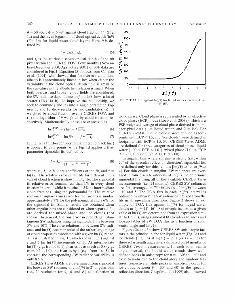
In angular bins where sunglint is strong (i.e., within20° of the specular reflection direction), sigmoidal fitsare defined only for thick clouds [ln( f ̃) � 1.4 or f ̃ �4]. For thin clouds in sunglint, SW radiances are aver-aged in four discrete intervals of ln( f ̃). To determinesigmoidal fits using all of the available CERES Terrameasurements (i.e., 24 months), CERES SW radiancesare first averaged in 750 intervals of ln( f ̃) between10 and 5. The TOA flux in each ln( f ̃) interval isobtained by integrating SW radiances inferred from thefits in all upwelling directions. Figure 2 shows an ex-ample of TOA flux against ln( f ̃) for liquid waterclouds at �o � 44°–46°. Anisotropic factors at a givenvalue of ln( f ̃) are determined from an expression simi-lar to Eq. (3), using sigmoidal fits to infer radiances andlookup tables of SW TOA flux as a function of solarzenith angle and ln( f ̃).

Figures 3a and 3b show CERES SW anisotropic fac-tors in the principal plane for liquid water (Fig. 3a) andice clouds (Fig. 3b) at ln( f ̃) � 2.01 (or f ̃ � 7.5) forthree solar zenith angle intervals based on 24 months ofCERES Terra measurements. In each solar zenithangle interval, the liquid water clouds show well-defined peaks in anisotropy for � � 30° to 60° andclose to nadir due to the cloud glory and rainbow fea-tures, respectively, while peaks in anisotropy occur forice clouds between � � 30° and 60° in the specularreflection direction. Chepfer et al. (1999) also observed

FIG. 2. TOA flux against ln( f ̃) for liquid water clouds at �o �44°–46°.


these features in multiangle Polarization and Direction-ality of Earth Reflectances (POLDER) measurementsand showed theoretically that these are likely due tohorizontally oriented ice crystals. Such pronounced mi-crophysical features were not present in ERBE andCERES TRMM ADMs because the angular bins usedto define those ADMs were too coarse.

b. Land and desert ADMs

1) CLEAR

Over clear land and desert, the CERES TRMMADMs were defined by grouping the InternationalGeosphere Biosphere Program (IGBP) global landcover types (Loveland and Belward 1997) over theTropics into four categories: low-to-moderate tree/shrub coverage, moderate-to-high tree/shrub coverage,dark desert, and bright desert. These categories wereassumed to apply over extensive geographical areas andremain invariant throughout the year. On a globalscale, this classification is inadequate because it doesnot account for vegetation types outside of the Tropics,many of which exhibit strong seasonal variations. Toimprove the spatial resolution of the clear land anddesert ADMs and account for changes in surface typewith season, the Terra ADMs over clear land and des-ert are defined for 1° latitude � 1° longitude equal arearegions, with a temporal resolution of 1 month. To gen-erate ADMs at these scales, all snow-free, clear-skyCERES Terra SW radiances from the available 24months of SSF data are first sorted by calendar monthand 1° latitude � 1° longitude equal area region. EachFOV radiance is converted to a reflectance as follows:

r��o, �, �� I��o, �, ��

�oEo�1 � se�

2, �9�

where �o � cos�o , Eo is the TOA solar irradiance(�1365 W m2) and (1 � �se) is the Earth–sun distancein astronomical units (AUs). A TOA normalized veg-

etation difference index (NDVI) for each CERES FOVis determined from PSF-weighted mean MODIS 0.63-(I0.63) and 0.86-�m (I0.86) radiances as follows:

NDVI �I0.86 I0.63

I0.86 � I0.63

. �10�

The TOA NDVI is used to separate subregions withina 1° latitude � 1° longitude region that have differentvegetation characteristics. Subregions with TOA NDVIdiffering by 0.1 or more are treated separately. Next, ifangular sampling within a region is sufficient, an eight-parameter nonparametric fit from Ahmad and Deering[1992, see their Eq. (37)] is applied to the CERES SWreflectances to represent the angular dependence in thereflectance field. The Bidirectional Reflectance Distri-bution Function (BRDF) used in the fit accounts formultiple scattering based on Chandrasekhar’s (1950)radiative transfer solution for a semi-infinite medium,and the so-called “hot spot” is modeled using an em-pirical term (Hapke 1986). Separate fits are derived forevery 0.2 increment in �o, provided that at least threeCERES FOVs are available in the following geome-tries: (i) � � 20°, (ii) � � 40° and � � 30°, (iii) � � 40°and 60° � � � 120°, and (iv) � � 40° and � � 150°. Ifthis condition is not satisfied, then CERES FOVs fromneighboring regions with the same IGBP type, NDVIand �o intervals are used to supplement the angularsampling. Only FOVs from neighboring regions within�15° latitude � �15° longitude are considered. If theviewing angle sampling criterion is still not satisfied,then a fit is not performed, and fluxes are determinedusing the CERES TRMM ADMs.

Figures 4a and 4b show the regional relative rms er-ror when the BRDF fits are applied to RAP and cross-track CERES data from December 2000 through Feb-ruary 2001 (Fig. 4a), and from June 2000 through Au-gust 2000 (Fig. 4b). Histograms of relative error andrelative rms error are provided in Figs. 5a–b. Overall,the relative rms error in reflectance from the BRDF fit

FIG. 3. CERES SW anisotropic factors in the principal plane for (a) liquid water and (b) iceclouds at ln( f ̃) � 2.01 (or f ̃ � 7.5) for three solar zenith angle intervals based on 24 monthsof CERES Terra measurements (negative � corresponds to � � 178°–180°; positive � corre-sponds to � � 0°–2°).


is between 6% and 7% for the two seasons. Relativeerrors tend to be larger over mountainous regions (e.g.,Rockies, Andes, Tibetan Plateau) and smaller over thebroadleaf forest regions of South America and over thecentral United States in summer.

To construct an ADM from the BRDF fits, albedosat several solar zenith angles in the interval of �o, inwhich the BRDF fit was derived, are first computed bydirectly integrating the BRDFs over � and �. Next, a fitbased on Rahman et al. (1993) is used to represent thealbedo dependence on solar zenith angle in each �o

interval. The instantaneous anisotropic factor at a given

location is inferred from the ratio of reflectance to al-bedo, both of which are evaluated from the above fits atthe FOV viewing geometry.

2) CLOUDS

The anisotropy of clouds over land and desert de-pends strongly upon cloud phase, cloud fraction, cloudoptical thickness, and the underlying surface type (es-pecially in thin or broken cloud conditions). CERESTRMM ADMs for clouds over land and desert weredefined for discrete classes of cloud phase, cloud frac-tion, and cloud optical depth for the four surface typesthat were used to define clear land CERES TRMMADMs. For CERES Terra, we use a similar approach tothat outlined over the ocean [section 4b(2)], with anadditional correction to account for surface reflection.Following Arking and Childs (1985), an observed radi-ance (I) is modeled as follows:

I��o, �, �� 1 f ��oEo

�clr��o, �, �� fIcld��o, �, ��

� f�oEo

� �clr��o, �, �� e��o e��

� �clrtcld��, �o�tcld��, ��

1 �clr�cld��, �11�

where the first term corresponds to reflection from thecloud-free area, the second term represents reflectionfrom the cloud, and the third and fourth terms corre-spond to scattering by the surface and atmospheretransmitted through the cloud, respectively; �clr is theclear-sky bidirectional reflectance, � � cos�, Icld is theradiance from the cloud layer, is the cloud opticaldepth, �clr and �cld are the clear-sky and cloud sphericalalbedos (Thomas and Stamnes 1999), respectively, andtcld is the diffuse transmittance of the cloud. Respec-tively, �clr and �clr are inferred from 1° BRDF fits; �cld

and tcld are determined from broadband radiative trans-fer model calculations using a highly modified versionof the model described in Fu and Liou (1993). In theradiative transfer model calculations, liquid waterclouds are assumed to have an effective droplet radiusof 10 �m, and ice clouds are assumed to have an effec-tive particle diameter of 60 �m. Lookup tables of �cld

and tcld are generated at 17 solar zenith angles and 19cloud optical depths.

Because I is known from the observations, Eq. (11)can be used to estimate the contribution from thecloudy area ( fIcld). Figure 6a shows an example of fIcld

against ln( f ̃) for the angular bins �o � 40°–45°, � �0°–5°, and � � 0°–5°. To generate this curve, allCERES measurements from 24 months for all land anddesert types were included and CERES radiances wereaveraged in 375 intervals of ln( f ̃). The relative rmserror in the sigmoid fit (solid line) is approximately 7%,

FIG. 4. Regional relative rms error in BRDF fits for RAP andcross-track CERES data from (a) Dec 2000 through Feb 2001 and(b) Jun 2000 through Aug 2000.

FIG. 5. Histograms of (a) 1° regional relative bias and (b) 1°regional relative rms error in BRDF fits for RAP and cross-trackCERES data from Dec 2000 through Feb 2001, and Jun 2000through Aug 2000.


Fig 4 live 4/C

comparable to what was obtained for clouds over theocean. Sigmoidal fits were also determined in all otherangular bins where CERES Terra observations occur.An angular resolution of 5° in �o, �, and � is used forland and desert. Separate fits were derived for liquidwater, and mixed and ice clouds, defined in section4a(2). Using fIcld, predicted from the sigmoidal fits to-gether with the 1° latitude � 1° longitude monthly clearland BRDF fits described in section 4b(1), the approxi-mation in Eq. (11) is used to construct ADMs for cloudsover land and desert that account for regional and sea-sonal changes in surface properties. The ADM flux isinferred by integrating Eq. (11):

F��o� � �1 f��oEo�clr��o� ��0

2� �0

1

fIcld��o, �, �� d�d�

� f�oEo��clr��o� e��o 2 �0

1

e��d�

� � clrtcld��, �o�t cld��

1 �clr�cld��, �12�

where �clr is the plane albedo and tcld is the sphericaltransmittance (ratio of transmitted flux to incident fluxfor an isotropic source). To reduce computation time,we assume �clr(�o , �, � ) � �clr(�o) in the third term ofEq. (12), thereby avoiding explicit double integrationover �clr(�o , �, �) e �� for every CERES FOV.

An anisotropic factor for an arbitrary FOV is deter-mined from radiance and flux estimates using Eqs. (11)and (12) with the appropriate clear-sky 1° BRDF fitsand sigmoidal curve. Figure 6b provides sample ADMsfor clear and cloudy conditions over a cropland/naturalvegetation mosaic surface (latitude � 36.52°N, longi-tude � 128.72°E) for �o � 59.24° on 2 December 2000.The cloud is composed of liquid water, covers 74% ofthe CERES FOV, and has a cloud optical depth of 5.2.The clear-sky case shows a markedly stronger backscat-ter contribution compared to the cloud case, which scat-

ters more radiation into the forward direction owing toits scattering phase function characteristics.

c. Snow and sea ice

One of the major differences in angular distributionmodel development for Terra compared with TRMM isthe availability of CERES RAP data over polar re-gions. Because the TRMM orbit is restricted to tropicallatitudes, there were not enough data to develop em-pirical snow ADMs for CERES TRMM. As a result,Loeb et al. (2003a) used theoretical ADMs to infer TOAfluxes over snow in tropical regions. Because Terra is asun-synchronous polar-orbiting satellite, CERES instru-ments on Terra measure radiances in polar regions fromvarious scene types and a wide range of viewing geom-etries. This allows the development of empirical ADMsto estimate radiative fluxes from snow and sea ice.

For convenience, snow/ice surfaces are divided intothree groups: permanent snow, fresh snow, and sea ice.Most permanent snow scenes occur over Antarcticaand Greenland, whereas fresh snow and sea ice occurover land and water, respectively. Because anisotropyalso varies with surface brightness (Loeb et al. 2003a),each of the three surface types are further stratified into“bright” and “dark” subclasses. A CERES FOV is de-termined to be bright or dark by comparing its geo-graphical location with a predetermined monthly re-gional snow map that classifies all 1° � 1° regions withsnow/sea ice as either bright or dark (Kato and Loeb2005). The snow maps are constructed as follows. (i)Using all available cloud-free CERES FOVs with snow/sea ice, mean MODIS 0.63-�m near-nadir (for � � 25°)reflectances are determined as a function of snow typeand solar zenith angle; (ii) every CERES FOV whoseMODIS 0.63-�m near-nadir reflectance lies below(above) the corresponding mean reflectance is assigneda value of 1 (�1); (iii) if the sum of all CERES FOVclassifications in a 1° � 1° region from 1 month of datais negative (positive), the region is classified as dark(bright). In this manner, 12 snow maps representingeach calendar month are produced.

To account for the effects of partial coverage by freshsnow or sea ice within a CERES FOV on anisotropy,bright and dark fresh snow and sea ice ADMs are fur-ther stratified into six intervals of fresh snow or sea icepercent coverage. When clouds are present, ADMs arefurther stratified by cloud fraction and cloud opticalthickness. Table 1 shows how the snow and sea iceADMs are defined for each surface type. The totalnumber of ADMs is 10 for permanent snow, 25 forfresh snow, and 25 for sea ice.

Following Loeb et al. (2003a), radiances measuredby CERES instruments are sorted into angular binsand averaged. Angular bin sizes are 2° for the solarzenith angle, and 5° for both viewing zenith and rela-tive azimuth angles over permanent snow. For freshsnow and sea ice, angle bin sizes are 5° for all threeangles. Radiances in undersampled angular bins are in-

FIG. 6. (a) Cloud SW radiance ( f Icld) against ln( f ̃) for cloudsover land and desert in angular bins �o � 40°–45°, � � 0°–5°, and� � 0°–5°. Solid line is a five-parameter sigmoid fit to the data. (b)Sample ADMs for clear and cloudy conditions over a cropland/natural vegetation mosaic surface (latitude � 36.52°N, longitude� 128.72°E) for �o � 59.24° on 2 Dec 2000. The cloud is composedof liquid water, covers 74% of the CERES FOV, and has a cloudoptical depth of 5.2.


ferred using the approach outlined in Loeb et al.(2003a).

Figures 7a–c show SW anisotropic factors for perma-nent snow (Fig. 7a), fresh snow (Fig. 7b), and sea ice(Fig. 7c) as a function of � for � � 0°–10° and � �170°–180°. When clouds are present over snow/sea ice,SW anisotropic factors show a greater dependence onviewing zenith angle than cloud-free scenes, especiallyin the forward scattering direction. Anisotropic factorsfor clear bright and dark surfaces are remarkably simi-lar over permanent snow, while the brighter surfaces

tend to be slightly more isotropic than dark scenes overfresh snow and sea ice.

d. Mixed-scene fields of view

Shortwave anisotropic factors for CERES FOVs thatlie over water–land–snow boundaries are determinedby accounting for the fractional coverage by each sur-face type as follows:

R��o, �, �� fWIW � fLIL � fSIS�

fWFW � fLFL � fSFS, �13�

TABLE 1. SW ADM scene-type definitions for permanent snow, fresh snow, and sea ice.

Surface type Cloud fraction Surface brightness Snow/sea ice fraction Cloud optical thickness

Permanent snow (10) 0.0–0.001 Bright, dark — —0.001–0.25 All — —

0.25–0.500.50–0.750.75–0.999

0.999–1.0 Bright, dark — Thin ( � 10), thick ( � 10)Fresh snow (25), sea ice (25) 0.0–0.01 All 0–0.01 —

0.01–0.250.25–0.500.50–0.750.75–0.99

Bright, dark 0.99–1.0 —0.01–0.25 All 0.0–0.01 —

0.01–0.250.25–0.500.50–0.750.75–0.99

0.25–0.50 All 0.0–0.01 —0.01–0.250.25–0.500.50–0.75

0.50–0.75 All 0.0–0.01 —0.01–0.250.25–0.50

0.75–0.99 All 0.0–0.01 —0.01–0.25

0.99–1.0 Bright, dark — Thin ( � 10), thick ( � 10)

FIG. 7. SW anisotropic factors against CERES viewing zenith angle near the principal plane for (a) permanent snow for �o � 62°–64°;(b) fresh snow for �o � 60°–65°; and (c) sea ice for �o � 60°–65°. “Clr” corresponds to clear; “Ovc” corresponds to overcast.


where fW, fL, and fS correspond to the fractional cov-erage over a CERES FOV by water, land, and snow,respectively; and IX and FX (X � W, L, S) are the meanradiance and TOA flux used to define ADMs for FOVswith 100% coverage by water, land, or snow.

e. Sunglint conditions

When a CERES FOV is over water and the satelliteviewing geometry is near the specular reflection direc-tion, the radiance-to-flux conversion is less reliable ow-ing to the large variability in ocean reflectance at thoseangles. To determine whether or not a footprint is tooclose to the specular reflection direction to provide areliable flux retrieval, the following expression is evalu-ated:

�R � �1 fice fcld��Rclr, �14�

where fice and fcld correspond to the fraction of theCERES FOV covered by sea ice and cloud, respec-tively, and �Rclr

is the standard deviation of clear oceananisotropic factors in angular bins adjacent to the ob-servation angle. If an observation falls in an angular binfor which �R � 0.05, a radiance-to-flux conversion isnot performed. Instead, a mean flux value, correspond-ing to the ADM scene type over the FOV, is used.ADM flux values are determined when the ADMs areconstructed by direct integration of the radiances forthe corresponding scene type.

5. LW and WN ADMsADMs for LW and WN scenes are defined in terms

of several surface and meteorological properties thatinfluence radiance anisotropy over the ocean, land, anddesert. In addition, because the cloud retrieval algo-rithm uses different approaches during the daytime andnighttime owing to the lack of visible imager informa-tion at night, separate LW and WN ADMs are devel-oped for daytime and nighttime conditions.

a. Clear ocean, land, and desert

To account for the increased variability in surfaceproperties encountered by Terra compared to TRMM,the number of surface types used to define land anddesert ADMs has been increased from two for TRMMto six for Terra. Table 2 provides the IGBP surfacetypes corresponding to each of the six land categories.These classes were determined by analyzing the spatialdistribution of surface emissivity (Wilber et al. 1999)over the different IGBP types.

In addition to surface type, the scene types are strati-fied into discrete intervals of precipitable water (w),vertical temperature change (�T), and imager-basedsurface skin temperature (Ts) (Table 3). Over water, wis obtained from SSM/I retrievals; over land and desert,w is obtained from meteorological values (DAO 1996).Here, �T is defined as the lapse rate in the first 300 hPaof the atmosphere above the surface. It is computed bysubtracting the DAO (1996) air temperature at the

pressure level that is 300 hPa below the surface pres-sure (i.e., surface pressure minus 300 hPa) from Ts; Ts isestimated from the clear-sky 11-�m radiance using anarrowband radiative transfer algorithm that uses tem-perature and humidity profile inputs from the GEOSDAS V4.0.3 (Minnis et al. 2003).

Longwave and WN ADMs are defined as a functionof viewing zenith angle using a 2° angular bin resolu-tion. Consequently, variations in anisotropy with solarzenith angle and relative azimuth angle are not ac-counted for. While this approximation is reasonable forthe ocean and for all surface types at night, it breaksdown during daytime for land areas with highly variabletopography (Minnis and Khaiyer 2000; Minnis et al.2004).

Figures 8a–d provide examples of LW ADMs for dif-ferent surface types as a function of surface skin tem-perature for w � 1 and �T between 15 and 30 K. For allsurface types, LW anisotropy increases as surface skintemperature increases. Because the WN channel ismore sensitive to surface skin temperature, WN anisot-ropy (not shown) is found to be significantly more pro-nounced than LW anisotropy. While LW and WN an-

TABLE 2. Surface-type definitions for clear-sky LW and WNADMs over the ocean, land, and desert.

ADM surface type IGBP type

Forests (1) Evergreen needleleaf(2) Evergreen broadleaf(3) Deciduous needleleaf(4) Deciduous broadleaf(5) Mixed

Savannas (8) Woody savannas(9) Savannas

Grasslands/cropland (6) Closed shrubland(10) Grasslands(11) Permanent wetlands(12) Croplands(13) Urban(14) Cropland/natural vegetation mosaics

Dark deserts (7) Open shrubland(18) Tundra

Bright deserts (16) Barren deserts

Ocean (17) Water bodies

TABLE 3. Precipitable water (w), lapse rate (�T ), and surfaceskin temperature (Ts) intervals used to determine LW and WNADMs under clear-sky conditions over the ocean, land, anddesert.

w (cm) �T (K) Ts (K)

0–1 �15 �2701–3 15–30 270–2903–5 30–45 290–310�5 �45 310–330

�330


isotropy also increases with �T, the sensitivity is lesspronounced than it is to Ts.

b. Clouds over the ocean, land, and desert

Under cloudy conditions, LW and WN anisotropydepends on several parameters, including surface type,w, Ts, surface–cloud temperature difference (�Tsc),cloud fraction, and cloud infrared emissivity (�c). Tocharacterize scenes in terms of these parameters, wedefine a “pseudoradiance” parameter � as follows:

�w, Ts, Tc, f, s, c� � �1 f �sB�Ts� � �j�1

2

�sB�Ts��1 cj� � cj

B�Tcj�� fj,

�15�

where fj is the cloud fraction of the jth cloud layerwithin a CERES FOV ( f � f1 � f2), Tcj

is the corre-sponding layer cloud-top temperature, �s is the surfaceinfrared emissivity, and B(T) � �1�T4 , where � is theStefan–Boltzmann constant (�5.6696 � 108 W m2

sr1 deg4). Here, �cjis determined from

cj� 1 e�aj, �16�

where ajis the infrared absorption cloud optical depth

of the jth layer derived using the approach outlined inMinnis et al. (1998) from visible cloud optical depth and

particle effective radius retrievals available on the SSFproduct. For a given surface type, and fixed intervals ofw, f, Ts, and �Tsc (Table 4), LW (and WN) radiancesshow a simple monotonic dependence on �. As an ex-ample, Fig. 9a shows LW radiances against � for threedifferent viewing bins over the ocean for w � 5 cm,Ts�300–305 K, �Tsc �85 K, and f�1.0. To produce Fig.9a, the observed LW radiances were averaged in 250 �bins of a width of 1 W m2 sr1. Note that because w,f, Ts, and �Tsc are held fixed when Eq. (15) is applied,the main source of variation in � is from �c For an

FIG. 8. LW anisotropic factors for clear scenes with w � 0.0–1.0 cm and �T � 15°–30°C; (a) ocean, (b) forests, (c) savannas, (d)cropland/grassland, (e) dark deserts, and (f) bright deserts.

FIG. 9. (a) LW radiance against � for � � 0°–2°, � � 30°–32°,and � � 68°–70° over the ocean for w � 5 cm, Ts � 300–305 K,�Tsc � 85 K, and f � 1.0. Solid line corresponds to a third-orderpolynomial fit to the data. (b) Anisotropic factor (R) againstCERES viewing zenith angle for � � 33.8 W m2 sr1 and � �95.8 W m2 sr1.


arbitrary CERES FOV, R is determined by first evalu-ating the radiance at � from Eq. (15) in each viewingzenith angle bin. The relationship between radianceand � in a given angular bin is derived from predeter-mined third-order polynomial fits in each � bin for theintervals of w, f, Ts, and �Tsc , shown in Table 4. Theradiances are then integrated over viewing zenith angleto produce an ADM flux and R is obtained directlyfrom Eq. (3). Figure 9b shows the viewing zenith angledependence of R at � � 33.8 W m2 sr1 and � � 95.8W m2 sr1 , corresponding to the conditions in Fig. 9a.At � � 33.8 W m2 sr1 , the cloud is thick (�c � 1) andthe viewing zenith angle dependence of R is weak. Thisis expected since the cloud top is located in the uppertroposphere where there is less attenuation above thecloud to cause appreciable limb darkening. At � � 95.8W m2 sr1 , the clouds are much thinner (�c � 0.4–0.5)and the LW anisotropy is more pronounced becausethe contribution from the warm ocean surface transmit-ted through the cloud is attenuated more rapidly withviewing zenith angle.

c. Snow

Longwave and WN ADMs over permanent snow,fresh snow, and sea ice are defined with an angularresolution of 2° in viewing zenith angle for 24 discretescene classes by clear fraction, surface skin tempera-ture, and surface–cloud top temperature difference(Table 5). Figures 10a–c show daytime LW ADMs forthe three surface types. As expected, LW ADMs forclear scenes with Ts � 250 K are more anisotropic thanthose with Ts � 250 K. Under cloudy conditions, largeranisotropy occurs when Ts � 250 K and �Tsc � 20 K.Clouds in this scene type are not completely opaqueclose to nadir, so that the difference in the effectivetemperature at nadir and the oblique viewing angle islarge. For � � 84°, the radiances show more variabilitybecause of reduced sampling and because part of theCERES FOV lies beyond the earth’s horizon (no sceneinformation is available from the imager over that partof the FOV). The uncertainty in TOA flux due to ra-diance uncertainties at � � 84° is �0.3 W m2.

6. Footprints with insufficient imager information

In circumstances where there is insufficient imagercoverage or scene information for a CERES FOV due

to missing MODIS data and/or missing cloud propertyretrievals, anisotropic factors are determined from theCERES radiances directly using a feed-forward errorback-propagation artificial neural network (ANN)simulation (Loukachine and Loeb 2003; Loukachineand Loeb 2004). This occurs when the total fraction ofunknown cloud properties over the footprint, as de-fined by Eq. (2) of Loeb et al. (2003a), is greater than0.35. The ANN has been trained using CERES TerraSSF data to provide a mapping between the CERESradiances and ADM-derived anisotropic factors overdifferent surface types (ocean, land, desert, and snow).Validation tests show that the root-mean-square (rms)difference between instantaneous SW TOA fluxes fromthe ANN and original ADMs is approximately 9% forSW, 3.5% for LW daytime, and 3% for LW nighttime(WN rms differences are similar). Globally, approxi-mately 5% of CERES TOA fluxes are inferred usingthe ANN scheme. The frequency of ANN use is signifi-cantly higher in mountainous regions, in coastal areas,and over snow/sea ice, where uncertainties in imager-derived cloud properties are larger. ANN is also fre-quently used at oblique CERES viewing zenith anglesin the cross-track direction because MODIS is limitedto cross-track viewing zenith angles that are smallerthan 63°.

7. Summary

To determine the earth’s radiation budget fromCERES, measured radiances at a given sun–Earth–satellite configuration must be converted to outgoingreflected solar and emitted thermal TOA radiativefluxes. CERES SW, LW, and WN ADMs are derivedfrom 24 months of global CERES Terra radiances, im-ager-derived cloud parameters from MODIS, and me-teorological information from the Global Modeling andAssimilation Office (GMAO)’s Goddard Earth Ob-serving System Data Assimilation System (DAS)V4.0.3 product. The ADM scene types are defined as afunction of scene parameters that have a strong influ-ence on the anisotropy (or angular variation) of theearth’s radiation field at the TOA.

For clear scenes over the ocean, CERES Terra SWADMs are defined as a function of wind speed and a

TABLE 4. Surface type, precipitable water (w), cloud fraction( f ), surface–cloud temperature difference (�Tsc), and surface skintemperature (Ts) intervals used to determine LW and WN ADMsunder cloudy conditions over the ocean, land, and desert.

Surfacetype

w(cm) f �Tsc (K ) Ts (K )

Ocean 0–1 0.001–0.5 �15; 15 to �275; 275 toLand 1–3 0.5–0.75 85 every 5 K; 320 every 5 KDesert 3–5 0.75–0.999 10–�85 �320

�5 0.999–1.0

TABLE 5. Clear fraction ( fclr), surface skin temperature (Ts),and surface–cloud temperature difference (�Tsc) intervals used todetermine LW and WN ADMs over permanent snow (PS), freshsnow, and sea ice.

fclr Ts (K ) �Tsc (K )

0.999 � fclr � 1.000 �2500.750 � fclr � 0.999 �250 �200.500 � fclr � 0.750 �200.250 � fclr � 0.500 �240 (PS, nighttime)0.100 � fclr � 0.250 �240 (PS, nighttime)fclr � 0.001


theoretical correction is used to account for aerosol op-tical depth variation. Over land and desert, clear ADMsare defined for 1° latitude � 1° longitude equal arearegions with a temporal resolution of 1 month. TheADMs are inferred from eight-parameter nonparamet-ric fits to the bidirectional reflectance distribution func-tion at these time and space scales. ADMs for clearscenes over snow/ice surfaces are stratified according towhether the surface is over permanent snow, freshsnow, or sea ice. Each of the three surface types arefurther stratified into “bright” and “dark” subclassesusing predetermined monthly regional snow maps thatclassify all 1° � 1° regions with snow/sea ice as eitherbright or dark. Shortwave ADMs under cloudy condi-tions over the ocean are defined as continuous func-tions of a cloud parameter determined from imager-based cloud fraction and cloud optical depth. A sigmoi-dal fit is used to provide a continuous mapping betweenthe cloud parameter and CERES radiances in each 2°angular bin interval in solar zenith angle, viewing zenithangle, and relative azimuth angle. Separate SW ADMsfor liquid water, mixed phase, and ice clouds are de-rived from the sigmoidal fits. A similar approach is usedto develop SW ADMs over land and desert, with addi-tional approximations to account for the anisotropy ofthe underlying surface. ADMs for clouds over snow/iceare defined for discrete classes of cloud fraction andcloud optical thickness.

In the LW and WN regions, ADMs under cloud-freeconditions are defined for one ocean class, five landcategories corresponding to groupings of major IGBPsurface types, and one snow class. The ocean and land

clear-sky ADMs are further stratified into discrete in-tervals of precipitable water, vertical temperaturechange, and imager-based surface skin temperature.Over snow, clear-sky ADMs are stratified by surfaceskin temperature. When clouds are present over theocean, land, or desert, the scene-type dependence ofLW and WN radiances is represented by a parameter-ization that is a function of precipitable water, surfaceand cloud-top temperature, surface and cloud emissiv-ity, and cloud fraction. Over snow, LW and WN ADMsare defined as a function of cloud fraction, surface skintemperature, and the temperature difference betweenthe surface and cloud top.

In Part II of this paper, SW, LW, and WN TOAfluxes derived from the CERES Terra ADMs are as-sessed through extensive validation tests similar tothose described in Loeb et al. (2003b). TOA fluxesfrom the new Terra ADMs will also be compared withTOA fluxes from the CERES TRMM ADMs and withfluxes based on algorithms developed during the EarthRadiation Budget Experiment (ERBE) (Smith et al.1986; Suttles et al. 1992).

Acknowledgments. This research was funded by theClouds and the Earth’s Radiant Energy System(CERES) project under NASA Grant NAG-1-2318.

REFERENCES

Ahmad, S. P., and D. W. Deering, 1992: A simple analytical func-tion for bidirectional reflectance. J. Geophys. Res., 97,18 867–18 886.

Arking, A., and J. D. Childs, 1985: Retrieval of cloud cover pa-

FIG. 10. Daytime LW anisotropic factors against CERES viewing zenith angle for (a) permanent snow, (b) fresh snow, and (c) seaice. “Clr” corresponds to clear; “Ovc” corresponds to overcast; Tsfc refers to surface skin temperature; Tcld corresponds to cloud-toptemperature.


rameters from multispectral satellite images. J. Climate Appl.Meteor., 24, 322–333.

Barnes, W. L., T. S. Pagano, and V. V. Salomonson, 1998: Pre-launch characteristics of the Moderate Resolution ImagingSpectroradiometer (MODIS) on EOS-AM1. IEEE Trans.Geosci. Remote Sens., 36, 1088–1100.

Cahalan, R. F., W. Ridgway, W. J. Wiscombe, T. L. Bell, and J. B.Snider, 1994: The albedo of fractal stratocumulus clouds. J.Atmos. Sci., 51, 2434–2455.

Cess, R. D., and Coauthors, 1990: Intercomparison and interpre-tation of climate feedback processes in 19 atmospheric gen-eral circulation models. J. Geophys. Res., 95, 16, 601–16, 615.

——, and Coauthors, 1996: Cloud feedback in atmospheric gen-eral circulation models: An update. J. Geophys. Res., 101,12 791–12 794.

Chandrasekhar, S., 1950: Radiative Transfer. Clarendon, 393 pp.Chepfer, H., G. B. Brogniez, P. Goloub, F. M. Breon, and P. H.

Flamant, 1999: Observations of horizontally oriented ice crys-tals in cirrus clouds with POLDER-1/ADEOS-1. J. Quant.Spectrosc. Radiat. Transfer, 63, 521–543.

Cubasch, U., and Coauthors, 2001: Projection of future climatechange. Climate Change 2001: The Scientific Basis, Contribu-tion of Working Group I to the Third Assessment Report ofthe Intergovernmental Panel on Climate Change, J. T. Hough-ton et al., Eds., Cambridge University Press, 527–582.

DAO, cited 1996: Algorithm Theoretical Basis Document forGoddard Earth Observing System Data Assimilation System(GEOS DAS) with a focus on version 2. [Available online athttp://gmao.gsfc.nasa.gov/systems/geos4/.]

Fu, Q., and K.-N. Liou, 1993: Parameterization of the radiativeproperties of cirrus clouds. J. Atmos. Sci., 50, 2008–2025.

Geier, E. B., R. N. Green, D. P. Kratz, P. Minnis, W. F. Miller, S.K. Nolan, and C. B. Franklin, cited 2001: Single satellite foot-print TOA/surface fluxes and clouds (SSF) collection docu-ment. [Available online at http://asd-www.larc.nasa.gov/ceres/collect_guide/SSF-CG.pdf.]

Goodberlet, M., C. Swift, and J. Wilkerson, 1990: Ocean surfacewind speed measurements of Special Sensor Microwave/Imager (SSM/I). IEEE Geosci. Remote Sens., GE-28, 828–832.

Hapke, B., 1986: Bidirectional reflectance spectroscopy, 4, Theextinction coefficient and the opposition effect. Icarus, 67,264–280.

Hess, M., P. Koepke, and I. Schult, 1998: Optical properties ofaerosols and clouds: The software package OPAC. Bull.Amer. Meteor. Soc., 79, 831–844.

Ignatov, A., and L. L. Stowe, 2002: Aerosol retrievals from indi-vidual AVHRR channels. Part I: Retrieval algorithm andtransition from Dave to 6S radiative transfer model. J. Atmos.Sci., 59, 313–334.

Kato, S., and N. G. Loeb, 2005: Top-of-atmosphere shortwavebroadband observed radiance and estimated irradiance fromClouds and the Earth’s Radiant Energy System (CERES)instruments on Terra over polar regions. J. Geophys. Res., inpress.

Kummerow, C., W. Barnes, T. Kozu, J. Shiue, and J. Simpson,1998: The Tropical Rainfall Measuring Mission (TRMM)sensor package. J. Atmos. Oceanic Technol., 15, 809–817.

Loeb, N. G., K. J. Priestley, D. P. Kratz, E. B. Geier, R. N. Green,B. A. Wielicki, P. O’R. Hinton, and S. K. Nolan, 2001: De-termination of unfiltered radiances from the Clouds and theEarth’s Radiant Energy System (CERES) instrument. J.Appl. Meteor., 40, 822–835.

——, S. Kato, and B. A. Wielicki, 2002: Defining top-of-atmosphere flux reference level for Earth radiation budgetstudies. J. Climate, 15, 3301–3309.

——, N. M. Smith, S. Kato, W. F. Miller, S. K. Gupta, P. Minnis,and B. A. Wielicki, 2003a: Angular distribution models fortop-of-atmosphere radiative flux estimation from the Cloudsand the Earth’s Radiant Energy System instrument on the

Tropical Rainfall Measuring Mission Satellite. Part I: Meth-odology. J. Appl. Meteor., 42, 240–265.

——, K. Loukachine, N. M. Smith, B. A. Wielicki, and D. F.Young, 2003b: Angular distribution models for top-of-atmosphere radiative flux estimation from the Clouds and theEarth’s Radiant Energy System instrument on the TropicalRainfall Measuring Mission Satellite. Part II: Validation. J.Appl. Meteor., 42, 1748–1769.

Loukachine, K., and N. G. Loeb, 2003: Application of an artificialneural network simulation for top-of-atmosphere radiativeflux estimation from CERES. J. Atmos. Oceanic Technol., 20,1749–1757.

——, and ——, 2004: Top-of-atmosphere flux retrievals fromCERES using artificial neural networks. J. Remote Sens. En-viron., 93, 381–390.

Loveland, T. R., and A. S. Belward, 1997: The International Geo-sphere Biosphere Programme Data and Information SystemGlobal Land Cover dataset (DISCover). Acta Astronaut., 41,681–689.

Minnis, P., and M. M. Khaiyer, 2000: Anisotropy of land surfaceskin temperature derived from satellite data. J. Appl. Me-teor., 39, 1117–1129.

——, D. P. Garber, D. F. Young, R. F. Arduini, and Y. Tokano,1998: Parameterizations of reflectance and effective emit-tance for satellite remote sensing of cloud properties. J. At-mos. Sci., 55, 3313–3339.

——, D. F. Young, S. Sun-Mack, P. W. Heck, D. R. Doelling, andQ. Trepte, 2003: CERES Cloud Property Retrievals fromImagers on TRMM, Terra, and Aqua. Proc. SPIE 10th Int.Symp. on Remote Sensing: Conf. on Remote Sensing ofClouds and the Atmosphere VII, Barcelona, Spain, 37–48.

——, A. V. Gambheer, and D. R. Doelling, 2004: Azimuthal an-isotropy of longwave and infrared window radiances fromCERES TRMM and Terra data. J. Geophys. Res., 109,D08202, doi:10.1029/2003JD004471.

Nakajima, T., and M. Tanaka, 1986: Matrix formulations for thetransfer of solar radiation in a plane-parallel scattering atmo-sphere. J. Quant. Spectrosc. Radiat. Transfer, 35, 13–21.

——, and ——, 1988: Algorithms for radiative intensity calcula-tions in moderately thick atmospheres using a truncation ap-proximation. J. Quant. Spectrosc. Radiat. Transfer, 40, 51–69.

Rahman, H., M. M. Verstraete, and B. Pinty, 1993: Coupled sur-face-atmosphere reflectance (CSAR) model 1. Model de-scription and inversion on synthetic data. J. Geophys. Res.,98, 20 779–20 789.

Remer, L. A., and Coauthors, 2005: The MODIS aerosol algo-rithm, products, and validation. J. Atmos. Sci., 62, 947–973.

Smith, G. L., 1994: Effects of time response on the point spreadfunction of a scanning radiometer. Appl. Opt., 33, 7031–7037.

——, R. N. Green, E. Raschke, L. M. Avis, J. T. Suttles, B. A.Wielicki, and R. Davies, 1986: Inversion methods for satellitestudies of the earth radiation budget: Development of algo-rithms for the ERBE mission. Rev. Geophys., 24, 407–421.

Suttles, J. T., B. A. Wielicki, and S. Vemury, 1992: Top-of-atmosphere radiative fluxes: Validation of ERBE scannerinversion algorithm using Nimbus-7 ERB data. J. Appl. Me-teor., 31, 784–796.

Thomas, G. E., and K. Stamnes, 1999: Radiative Transfer in theAtmosphere and Ocean. Cambridge University Press, 517 pp.

Wielicki, B. A., B. R. Barkstrom, E. F. Harrison, R. B. Lee III, G.L. Smith, and J. E. Cooper, 1996: Clouds and the Earth’sRadiant Energy System (CERES): An Earth observing sys-tem experiment. Bull. Amer. Meteor. Soc, 77, 853–868.

Wilber, A. C., D. P. Kratz, and S. K. Gupta, 1999: Surface emis-sivity maps for use in satellite retrievals of longwave radia-tion. NASA Tech. Rep. TP-1999-209362, 35 pp.

Young, D. F., P. Minnis, D. R. Doelling, G. G. Gibson, and T.Wong, 1998: Temporal interpolation methods for the Cloudsand the Earth’s Radiant Energy System (CERES) experi-ment. J. Appl. Meteor., 37, 572–590.


Documents

Angular Distribution Models for Top-of-Atmosphere