Embed Size (px)
Citation preview
Advanced Review
Anomaly detection in dynamicnetworks: a surveyStephen Ranshous,1,2 Shitian Shen,1,2 Danai Koutra,3 SteveHarenberg,1,2 Christos Faloutsos3 and Nagiza F. Samatova1,2∗
Anomaly detection is an important problem with multiple applications, and thushas been studied for decades in various research domains. In the past decade therehas been a growing interest in anomaly detection in data represented as networks,or graphs, largely because of their robust expressiveness and their natural abilityto represent complex relationships. Originally, techniques focused on anomalydetection in static graphs, which do not change and are capable of representingonly a single snapshot of data. As real-world networks are constantly changing,there has been a shift in focus to dynamic graphs, which evolve over time.
In this survey, we aim to provide a comprehensive overview of anomalydetection in dynamic networks, concentrating on the state-of-the-art methods. Wefirst describe four types of anomalies that arise in dynamic networks, providingan intuitive explanation, applications, and a concrete example for each. Havingestablished an idea for what constitutes an anomaly, a general two-stage approachto anomaly detection in dynamic networks that is common among the methods ispresented. We then construct a two-tiered taxonomy, first partitioning the methodsbased on the intuition behind their approach, and subsequently subdividingthem based on the types of anomalies they detect. Within each of the tier onecategories—community, compression, decomposition, distance, and probabilisticmodel based—we highlight the major similarities and differences, showing thewealth of techniques derived from similar conceptual approaches. © 2015 The Authors.WIREs Computational Statistics published by Wiley Periodicals, Inc.
How to cite this article:WIREs Comput Stat 2015. doi: 10.1002/wics.1347
Keywords: anomaly detection; dynamic networks; outlier detection; graph min-ing; dynamic network anomaly detection; network anomaly detection
INTRODUCTION
Anetworka is a powerful way to represent acollection of objects and the relationships or
connections among them. Examples include global
∗Correspondence to: [email protected] of Computer Science, North Carolina State University,Raleigh, NC, USA2Computer Science and Mathematics Division, Oak Ridge NationalLaboratory, Oak Ridge, TN, USA3Computer Science Department, Carnegie Mellon University, Pitts-burgh, PA, USA
Conflict of interest: The authors have declared no conflicts of interestfor this article.
financial systems connecting banks across the world,electric power grids connecting geographically dis-tributed areas, and social networks that connect users,businesses, or customers using relationships suchas friendship, collaboration, or transactional inter-actions. These are examples of dynamic networks,which, unlike static networks, are constantly under-going changes to their structure or attributes. Possi-ble changes include insertion and deletion of vertices(objects), insertion and deletion of edges (relation-ships), and modification of attributes (e.g., vertex oredge labels).
An important problem over dynamic networks isanomaly detection—finding objects, relationships, or
© 2015 The Authors. WIREs Computational Statistics published by Wiley Periodicals, Inc.This is an open access article under the terms of the Creative Commons Attribution-NonCommercial License, which permits use, distribution and reproductionin any medium, provided the original work is properly cited and is not used for commercial purposes.
Advanced Review wires.wiley.com/compstats
points in time that are unlike the rest. There are manyhigh-impact and practical applications of anomalydetection spanning numerous domains. A small sam-ple includes: detection of ecological disturbances,such as wildfires1,2 and cyclones3; intrusion detectionfor individual systems4 and network systems5–7; iden-tifying abnormal users and events in communicationnetworks8,9; and detecting civil unrest using twitterfeeds.10
The ubiquitousness and importance of anomalydetection in dynamic networks has led to the emer-gence of dozens of methods over the last 5 years(see Tables 3 and 4). These methods complementtechniques for static networks,11–14 as the latter oftencannot be easily adopted for dynamic networks.When considering the dynamic nature of the data,new challenges are introduced, including:
• New types of anomalies are introduced as a resultof the graph evolving over time, for example,splitting, disappearing, or flickering communi-ties.
• New graphs or updates that arrive over timeneed to be stored and analyzed. Storing all thenew graphs in their entirety can vastly increasethe size of the data. Therefore, typical offlineanalysis, where multiple passes over the data areacceptable and all of the data are assumed tofit into memory, becomes infeasible. Conversely,storing only the most recent graph or updatesrestricts the analysis to a single point in time.
• Graphs from different domains, such as socialnetworks compared to gene networks, mayexhibit entirely different behavior over time.This divergence in evolution can lead toapplication-specific anomalies and approaches.
• Anomalies, particularly those that are slow todevelop and span multiple time steps, can be hardto differentiate from organic graph evolution.
No dedicated and comprehensive survey ofanomaly detection in dynamic networks exists, despitethe growing importance of the topic because of theincreasing availability of network data. Althoughanomaly detection has been surveyed in a variety ofdomains,15–19 it has only recently been touched uponin the context of dynamic networks.20–22
In this survey, we hope to bridge the gapbetween the increasing number of methods foranomaly detection in dynamic networks and thelack of their comprehensive analysis. First, we give abroad overview of the related work in graph mining,anomaly detection, and the high-level approaches
used in the papers we discuss. We then introduce fourdifferent types of anomalies that these algorithmsdetect, namely, anomalous vertices, edges, subgraphs,and events. We continue with an extensive overviewof the existing methods based on the proposed tax-onomy, illustrated in Figure 5 that takes into accounttheir underlying design principles, such as those basedon graph communities, compression, decomposition,distance metrics, and probabilistic modeling of graphfeatures. Each taxonomic group is then subcatego-rized further based on the types of anomalies detected.Finally, we end with a more in-depth discussion ofthe methods that have code publicly available (seeTable 6), highlighting pros and cons of each.
BACKGROUND
Anomaly, or outlier, detection is a problem that spansmany domains. Chandola et al.16 provide an excellentoverview, taxonomy, and analysis of a multitudeof techniques (e.g., classification, clustering, andstatistical) for a variety of domains, expanding thework of Hodge et al.23 and Agyemang et al.24 As ourfocus will be on graphs, it is important to have abasic understanding of graph theory. West et al.25 andBalakrishnan et al.26 both offer comprehensive andapproachable introductions to graph theory, coveringall of the basics required for this survey and wellbeyond. Cook and Holder27 show how the theoreticalconcepts can be applied for graph mining, and recentlySamatova et al.28 provide an overview of many graphmining techniques as well as implementation detailsin the R programming language.b Owing to spacelimitations we cannot provide an introduction to thefundamentals of the types of methods we discuss, sowe provide references for introductory and overviewmaterial for each of them in Table 1.
It is important to note that in many domainsthe data are naturally represented as a network, withthe vertices and edges clearly defined. However, in
TABLE 1 Introductory and Overview References
Method References
Community detection Fortunato,29 Lancichinetti andFortunato,30 Reichardt andBornholdt,31 Harenberg et al.32
MDL and compression Rissanen,33–35 Grünwald36
Decomposition Golub and Reinsch,37 Klema andLaub,38 Kolda and Bader39
Distance Gao et al.,40 Rahm andBernstein,41 Cook and Holder27
Probabilistic Koller and Friedman,42 Glaz43
© 2015 The Authors. WIREs Computational Statistics published by Wiley Periodicals, Inc.
WIREs Computational Statistics Anomaly detection in dynamic networks
some cases, how to represent the data as a networkis unclear and can depend on the specific researchquestion being asked. The conversion processes usedin specific domains are outside the scope of this survey,and we assume all data are already represented asdynamic networks.
TYPES OF ANOMALIES
In this section, we identify and formalize four typesof anomalies that arise in dynamic networks. Thesecategories represent the output of the methods, notthe implementation details of how they detect theanomalies, e.g., comparing consecutive time points,using a sliding window technique. Note that oftentimes in real-world graphs, (e.g., social and biologicalnetworks) the graph’s vertex set V is called a set ofnodes. However, to avoid confusion with nodes ina physical computer network, and to align with theabstract mathematical representation, we call it a setof vertices.
Because the graphs are assumed to be dynamic,vertices and edges can be inserted or removed at everytime step. For the sake of simplicity, we assume thatthe vertex correspondence and the edge correspon-dence across different time steps are resolved becauseof unique labeling of vertices and edges, respectively.We define a graph series G as an ordered set of graphswith a fixed number of time steps. Formally, G ={
Gt
}Tt=1, where T is the total number of time steps,
Gt = (Vt, Et ⊆ (Vt ×Vt)), and the vertex set Vt and edgeset Et may be plain or attributed (labeled). Graphseries where T →∞ are called graph streams. The fullset of notations can be found in Table 2. In the fol-lowing subsections, we start with an intuitive expla-nation of the problem definition, then give a generalformal definition of the anomaly type, continue with
TABLE 2 Notation Summary
Symbol Meaning
G Graph series with a fixed number of time points
Gt Snapshot of the graph series at time t
Gs The sth graph segment, a grouping of temporallyadjacent graphs
It Vertex partitioning at time t, separating all thevertices into disjoint sets
V t Vertex set for the graph at time point t
vi Vertex i
Et Edge set for the graph at time point t
ei,j Edge between vi and vj
c0 Threshold value for normal versus anomalous data
some applications, and conclude with a representativeexample.
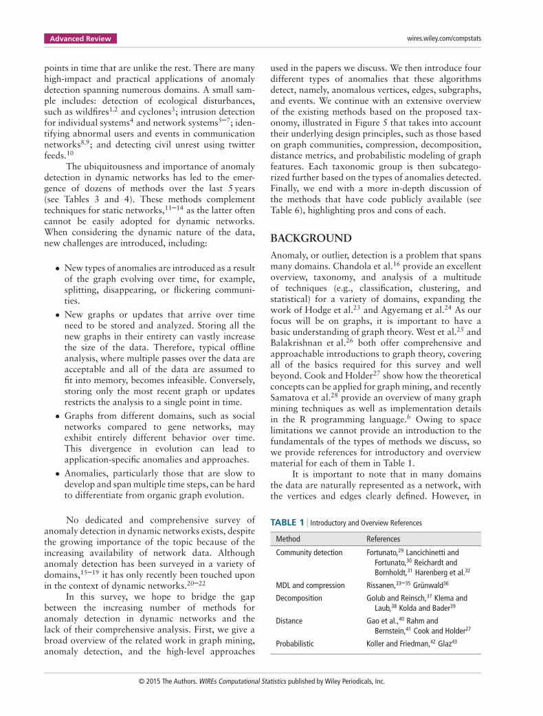
Type 1: Anomalous VerticesAnomalous vertex detection aims to find a subsetof the vertices such that every vertex in the subsethas an ‘irregular’ evolution compared to the othervertices in the graph. Optionally, the time point(s)where the vertices are determined to be anomalouscan be identified. What constitutes irregular behavioris dependent on the specific method, but it can begeneralized by assuming that each method providesa function that scores each vertex’s behavior, e.g.,measuring the change in the degree of a vertex fromtime step to time step. In static graphs, the singlesnapshot allows only intragraph comparisons to bemade, such as finding vertices with an abnormalegonet density.11 Dynamic graphs allow the temporaldynamics of the vertex to be included, introducing newtypes of anomalies that are not present in static graphs.A high-level definition for a set of anomalous verticesis as follows.
Definition 1. (Anomalous vertices). Given G, thetotal vertex set V = ∪T
t=1Vt, and a specified scoringfunction f : V→ℝ, the set of anomalous vertices V′ ⊆Vis a vertex set such that ∀ v′ ∈V′, |f (v′) − f̂| > c0,
where f̂ is a summary statistic of the scores f(v),∀ v∈V.
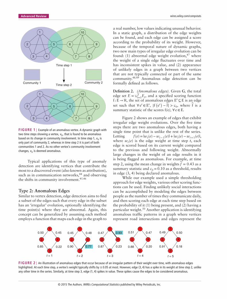
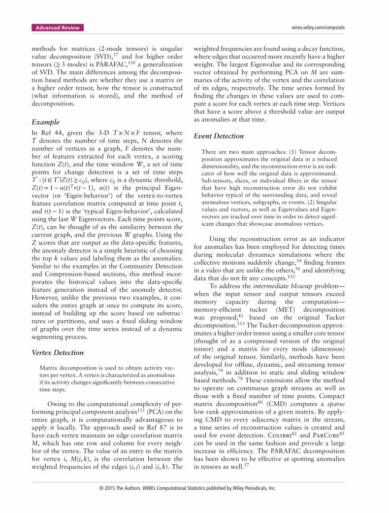
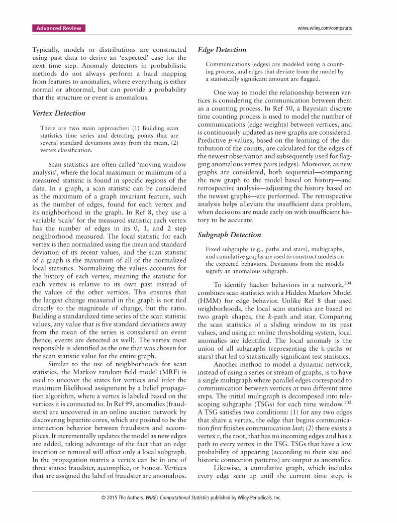
An example of an anomalous vertex is shownin Figure 1. Two time steps are shown, both with10 vertices and 2 communities. In this example,anomalous vertices are those that have a substantialchange in their community involvement comparedto the rest of the vertices in the graph. As v6 is theonly vertex that has any change in its communityinvolvement, it is labeled as an anomaly. Formally, wecan measure the change in community involvementbetween adjacent time steps t and t− 1 by lettingf(v) =
∑|C|i=1 ct−1
i,v ⊕ cti,v, where C= {c1, c2, … , c|C|} is
the set of communities, cti,v = 1 if v is part of commu-
nity ci at time step t and 0 otherwise, and ⊕ is the xoroperator.
The scoring function f will depend on the appli-cation. In the example shown in Figure 1, the ver-tices were scored based on the change in communityinvolvement. However, if the objective is identifyingcomputers on a network that become infected andpart of a botnet, then an appropriate scoring functionmight be measuring the change in the number of edgeseach vertex has between time steps, or the change inthe weights of the edges.
© 2015 The Authors. WIREs Computational Statistics published by Wiley Periodicals, Inc.
Advanced Review wires.wiley.com/compstats
Time step 1
Time step 2Community 2Community 1
1
2
3 4
5
1
2
3 4
5
6
10
9
87
6
10
9
87
FIGURE 1 | Example of an anomalous vertex. A dynamic graph withtwo time steps showing a vertex, v6, that is found to be anomalousbased on its change in community involvement. In time step 1, v6 isonly part of community 2, whereas in time step 2 it is part of bothcommunities 1 and 2. As no other vertex’s community involvementchanges, v6 is deemed anomalous.
Typical applications of this type of anomalydetection are identifying vertices that contribute themost to a discovered event (also known as attribution),such as in communication networks,44 and observingthe shifts in community involvement.45,46
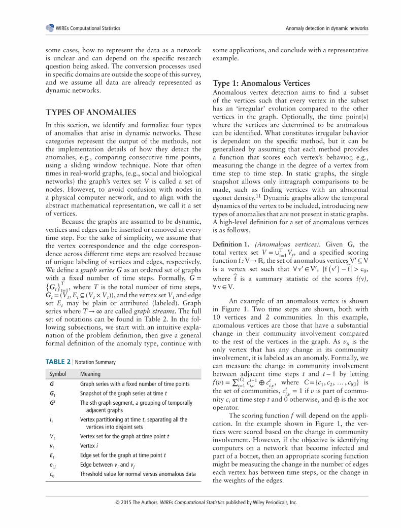
Type 2: Anomalous EdgesSimilar to vertex detection, edge detection aims to finda subset of the edges such that every edge in the subsethas an ‘irregular’ evolution, optionally identifying thetime point(s) where they are abnormal. Again, thisconcept can be generalized by assuming each methodemploys a function that maps each edge in the graph to
0.45 0.45 0.48 0.47 0.93 0.51 0.47 0.49 0.50
0.180.91
t = 5t = 4t = 3t = 2t = 1
0.200.880.230.870.77
0.50
3
42
1
3
42
1
3
42
1
3
42
1
3
42
1
0.22 0.900.85
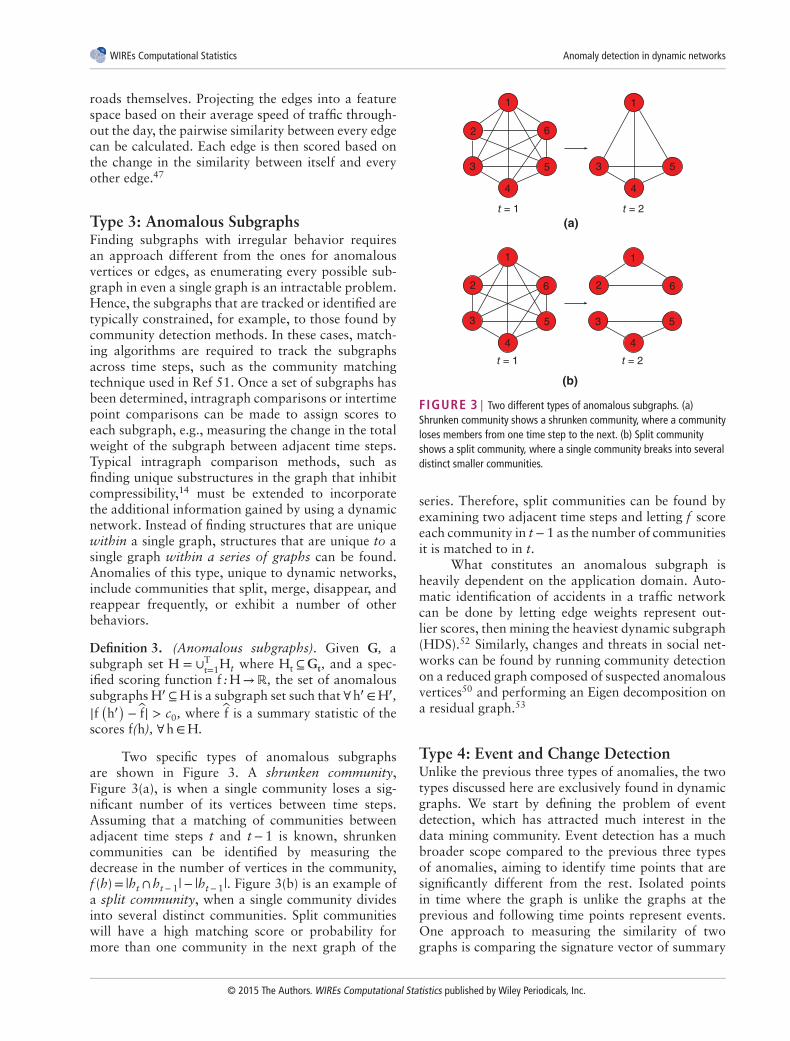
FIGURE 2 | An illustration of anomalous edges that occur because of an irregular pattern of their weight over time, with anomalous edgeshighlighted. At each time step, a vertex’s weight typically shifts by ± 0.05 at most. However, edge (3, 4) has a spike in its weight at time step 2, unlikeany other time in the series. Similarly, at time step 3, edge (1, 4) spikes in value. These spikes cause the edges to be considered anomalous.
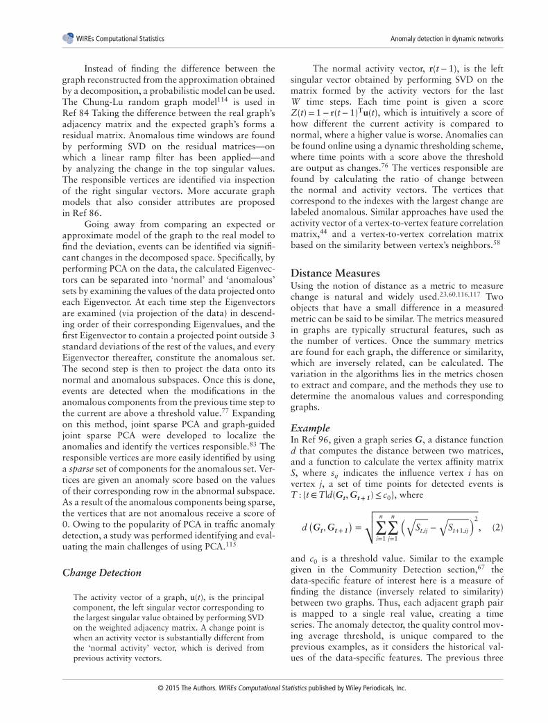
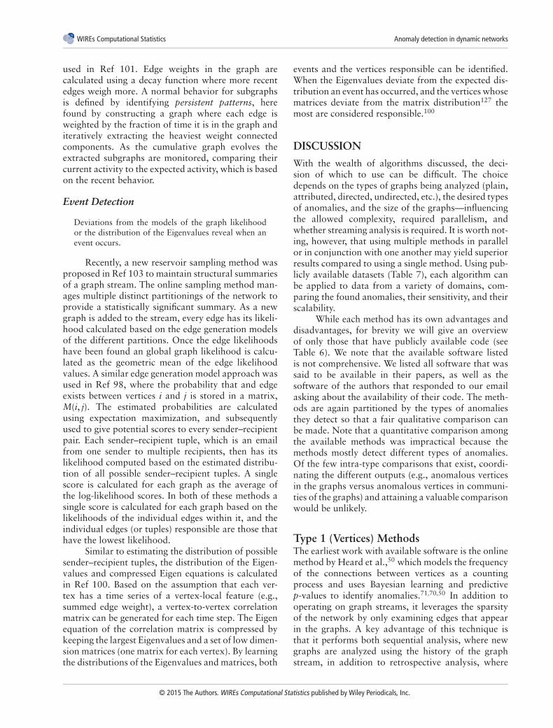
a real number, low values indicating unusual behavior.In a static graph, a distribution of the edge weightscan be found, and each edge can be assigned a scoreaccording to the probability of its weight. However,because of the temporal nature of dynamic graphs,two new main types of irregular edge evolution can befound: (1) abnormal edge weight evolution,47 wherethe weight of a single edge fluctuates over time andhas inconsistent spikes in value, and (2) appearanceof unlikely edges in a graph between two verticesthat are not typically connected or part of the samecommunity.48,49 Anomalous edge detection can beformally defined as follows.
Definition 2. (Anomalous edges). Given G, the totaledge set E = ∪T
t=1Et, and a specified scoring functionf : E→ℝ, the set of anomalous edges E′ ⊆E is an edgeset such that ∀ e′ ∈E′, |f (e′) − f̂| > c0, where f̂ is asummary statistic of the scores f(e), ∀ e∈E.
Figure 2 shows an example of edges that exhibitirregular edge weight evolutions. Over the five timesteps there are two anomalous edges, both having asingle time point that is unlike the rest of the series.Letting f (e)= |wt(e)−wt−1(e)|+ |wt(e)−wt+ 1(e)|,where wt(e) is the edge weight at time step t, eachedge is scored based on its current weight comparedto the previous and following weight. Abnormallylarge changes in the weight of an edge results in itis being flagged as anomalous. For example, at timestep 2, using the mean change in weights f̂ = 0.43 as asummary statistic and c0 =0.10 as a threshold, resultsin edge (3, 4) being declared anomalous.
While our example used a simple thresholdingapproach for edge weights, various other scoring func-tions can be used. Finding unlikely social interactionscan be accomplished by modeling the edges betweenpeople as the number of times they communicate daily,and then scoring each edge at each time step based onthe probability of it (1) being present, and (2) having aparticular weight.50 Another application is identifyinganomalous traffic patterns in a graph where verticesrepresent road intersections and edges represent the
© 2015 The Authors. WIREs Computational Statistics published by Wiley Periodicals, Inc.
WIREs Computational Statistics Anomaly detection in dynamic networks
roads themselves. Projecting the edges into a featurespace based on their average speed of traffic through-out the day, the pairwise similarity between every edgecan be calculated. Each edge is then scored based onthe change in the similarity between itself and everyother edge.47
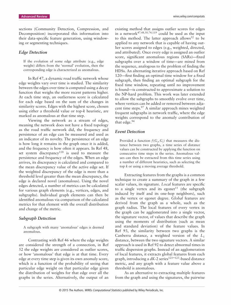
Type 3: Anomalous SubgraphsFinding subgraphs with irregular behavior requiresan approach different from the ones for anomalousvertices or edges, as enumerating every possible sub-graph in even a single graph is an intractable problem.Hence, the subgraphs that are tracked or identified aretypically constrained, for example, to those found bycommunity detection methods. In these cases, match-ing algorithms are required to track the subgraphsacross time steps, such as the community matchingtechnique used in Ref 51. Once a set of subgraphs hasbeen determined, intragraph comparisons or intertimepoint comparisons can be made to assign scores toeach subgraph, e.g., measuring the change in the totalweight of the subgraph between adjacent time steps.Typical intragraph comparison methods, such asfinding unique substructures in the graph that inhibitcompressibility,14 must be extended to incorporatethe additional information gained by using a dynamicnetwork. Instead of finding structures that are uniquewithin a single graph, structures that are unique to asingle graph within a series of graphs can be found.Anomalies of this type, unique to dynamic networks,include communities that split, merge, disappear, andreappear frequently, or exhibit a number of otherbehaviors.
Definition 3. (Anomalous subgraphs). Given G, asubgraph set H = ∪T
t=1Ht where Ht ⊆Gt, and a spec-ified scoring function f : H→ℝ, the set of anomaloussubgraphs H′ ⊆H is a subgraph set such that ∀ h′ ∈H′,|f (h′) − f̂| > c0, where f̂ is a summary statistic of thescores f(h), ∀ h∈H.
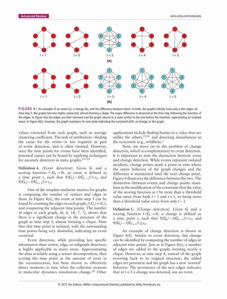
Two specific types of anomalous subgraphsare shown in Figure 3. A shrunken community,Figure 3(a), is when a single community loses a sig-nificant number of its vertices between time steps.Assuming that a matching of communities betweenadjacent time steps t and t−1 is known, shrunkencommunities can be identified by measuring thedecrease in the number of vertices in the community,f (h)= |ht ∩ht−1|− |ht− 1|. Figure 3(b) is an example ofa split community, when a single community dividesinto several distinct communities. Split communitieswill have a high matching score or probability formore than one community in the next graph of the
t = 1
3
4
5 3
4
5
6
1 1
2
(a)
(b)
3
4
5
6
1
2
3
4
5
6
1
2
t = 2
t = 1 t = 2
FIGURE 3 | Two different types of anomalous subgraphs. (a)Shrunken community shows a shrunken community, where a communityloses members from one time step to the next. (b) Split communityshows a split community, where a single community breaks into severaldistinct smaller communities.
series. Therefore, split communities can be found byexamining two adjacent time steps and letting f scoreeach community in t− 1 as the number of communitiesit is matched to in t.
What constitutes an anomalous subgraph isheavily dependent on the application domain. Auto-matic identification of accidents in a traffic networkcan be done by letting edge weights represent out-lier scores, then mining the heaviest dynamic subgraph(HDS).52 Similarly, changes and threats in social net-works can be found by running community detectionon a reduced graph composed of suspected anomalousvertices50 and performing an Eigen decomposition ona residual graph.53
Type 4: Event and Change DetectionUnlike the previous three types of anomalies, the twotypes discussed here are exclusively found in dynamicgraphs. We start by defining the problem of eventdetection, which has attracted much interest in thedata mining community. Event detection has a muchbroader scope compared to the previous three typesof anomalies, aiming to identify time points that aresignificantly different from the rest. Isolated pointsin time where the graph is unlike the graphs at theprevious and following time points represent events.One approach to measuring the similarity of twographs is comparing the signature vector of summary
© 2015 The Authors. WIREs Computational Statistics published by Wiley Periodicals, Inc.
Advanced Review wires.wiley.com/compstats
t = 1
5
6
1
2
3
4
5
6
1
2
3
4
5
6
1
2
3
4
5
6
1
2
3
4
5
6
1
2
3
4
5
6
1
2
3
4
5
6
1
2
3
4
5
6
1
2
3
4
5
6
1
2
3
4
5
6
1
2
3
4
(a)
(b)
t = 2 t = 3 t = 4 t = 5
t = 1 t = 2 t = 3 t = 4 t = 5
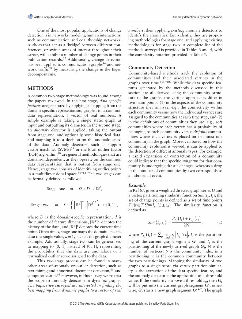
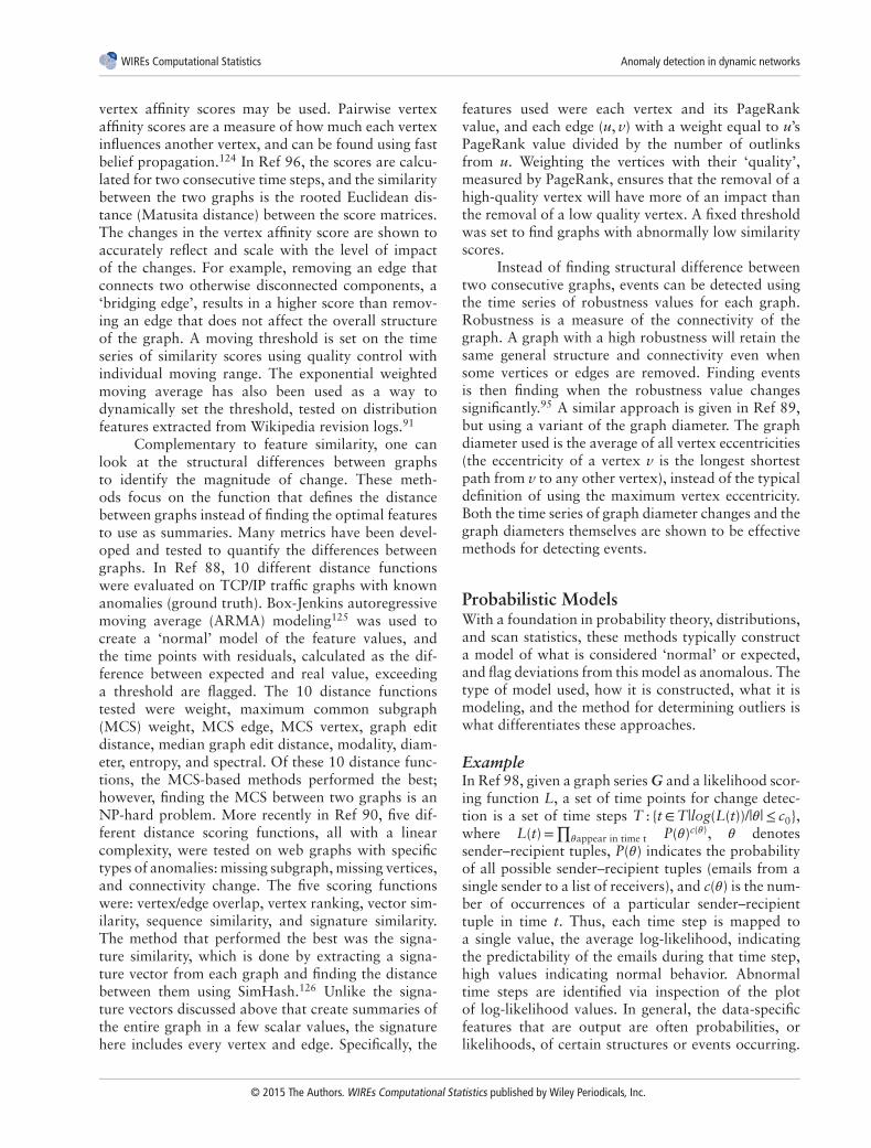
FIGURE 4 | An example of an event (a), a change (b), and the difference between them. In both, the graphs initially have only a few edges. Attime step 3, the graphs become highly connected, almost forming a clique. The major difference is observed at the time step following the insertion ofthe edges. In Figure 4(a) the edges are then removed and the graph returns to a state similar to the one before the insertion, representing an isolatedevent. In Figure 4(b), however, the graph maintains its new state indicating the sustained shift, or change, in the graph.
values extracted from each graph, such as averageclustering coefficient. The task of attribution—findingthe cause for the event—is not required as partof event detection, and is often omitted. However,once the time points for events have been identified,potential causes can be found by applying techniquesfor anomaly detection in static graphs.11–14
Definition 4. (Event detection). Given G and ascoring function f : Gt →ℝ, an event is defined asa time point t, such that |f(Gt)− f(Gt− 1)|> c0 and|f(Gt)− f(Gt+1)|> c0.
One of the simplest similarity metrics for graphsis comparing the number of vertices and edges inthem. In Figure 4(a), the event at time step 3 can befound by counting the edges in each graph, f (Gt)= |Et|,and comparing the adjacent time points. The numberof edges in each graph, {6, 6, 14, 7, 7}, shows thatthere is a significant change in the structure of thegraph at time step 3, almost forming a clique. Notethat this time point is isolated, with the surroundingtime points being very dissimilar, indicating an eventoccurred.
Event detection, while providing less specificinformation than vertex, edge, or subgraph detection,is highly applicable in many areas. Approximatingthe data available using a tensor decomposition, thenscoring the time point as the amount of error inthe reconstruction, has been shown to effectivelydetect moments in time when the collective motionsin molecular dynamics simulations change.54 Other
applications include finding frames in a video that areunlike the others,55,56 and detecting disturbances inthe ecosystem (e.g., wildfires).1
Now, we move on to the problem of changedetection, which is complementary to event detection.It is important to note the distinction between eventand change detection. While events represent isolatedincidents, change points mark a point in time wherethe entire behavior of the graph changes and thedifference is maintained until the next change point,Figure 4 illustrates the difference between the two. Thedistinction between events and change points mani-fests in the modification of the constraint that the valueof the scoring function at t be more than a thresholdvalue away from both t−1 and t+1, to being morethan a threshold value away from only t−1.
Definition 5. (Change detection). Given G and ascoring function f : Gt →ℝ, a change is defined asa time point t, such that |f(Gt)− f(Gt− 1)|> c0 and|f(Gt)− f(Gt+1)|≤ c0.
An example of change detection is shown inFigure 4(b). Similar to event detection, this changecan be identified by comparing the number of edges atadjacent time points. Just as in Figure 4(a), a numberof edges are added to the graph, forming nearly aclique. However, at time step 4, instead of the graphreverting back to its original structure, the addededges are persistent and the graph has a new ‘normal’behavior. The persistence of the new edges indicatesthat at t= 3 a change was detected, not an event.
© 2015 The Authors. WIREs Computational Statistics published by Wiley Periodicals, Inc.
WIREs Computational Statistics Anomaly detection in dynamic networks
One of the most popular applications of changedetection is in networks modeling human interactions,such as communication and coauthorship networks.Authors that act as a ‘bridge’ between different con-ferences, or switch areas of interest throughout theircareer, will exhibit a number of change points in theirpublication records.57 Additionally, change detectionhas been applied to communication graphs44 and net-work traffic58 by measuring the change in the Eigendecompositions.
METHODS
A common two-stage methodology was found amongthe papers reviewed. In the first stage, data-specificfeatures are generated by applying a mapping from thedomain-specific representation, graphs, to a commondata representation, a vector of real numbers. Asimple example is taking a single static graph asinput and outputting its diameter. In the second stage,an anomaly detector is applied, taking the outputfrom stage one, and optionally some historical data,and mapping it to a decision on the anomalousnessof the data. Anomaly detectors, such as supportvector machines (SVMs)59 or the local outlier factor(LOF) algorithm,60 are general methodologies that aredomain-independent, as they operate on the commondata representation that is output from stage one.Hence, stage two consists of identifying outlier pointsin a multidimensional space.60–64 The two stages canbe formally defined as follows:
Stage one ⇒ Ω ∶ D → ℝd,
Stage two ⇒ f ∶{[
ℝd]∗
,[ℝd
]t}
→ {0,1} ,
where D is the domain-specific representation, d isthe number of feature dimensions, [ℝd]* denotes thehistory of the data, and [ℝd]t denotes the current timepoint. Often times, stage one maps the domain-specificdata to a single value, d= 1, such as the graph diameterexample. Additionally, stage two can be generalizedto mapping to [0, 1] instead of {0, 1}, representingthe probability that the data are anomalous or anormalized outlier score assigned to the data.
This two-stage process can be found in manyother areas of anomaly or outlier detection, such astext mining and abnormal document detection,65 andcomputer vision.66 However, in this survey we restrictthe scope to anomaly detection in dynamic graphs.The papers we surveyed are interested in finding thebest mapping from dynamic graphs to a vector of real
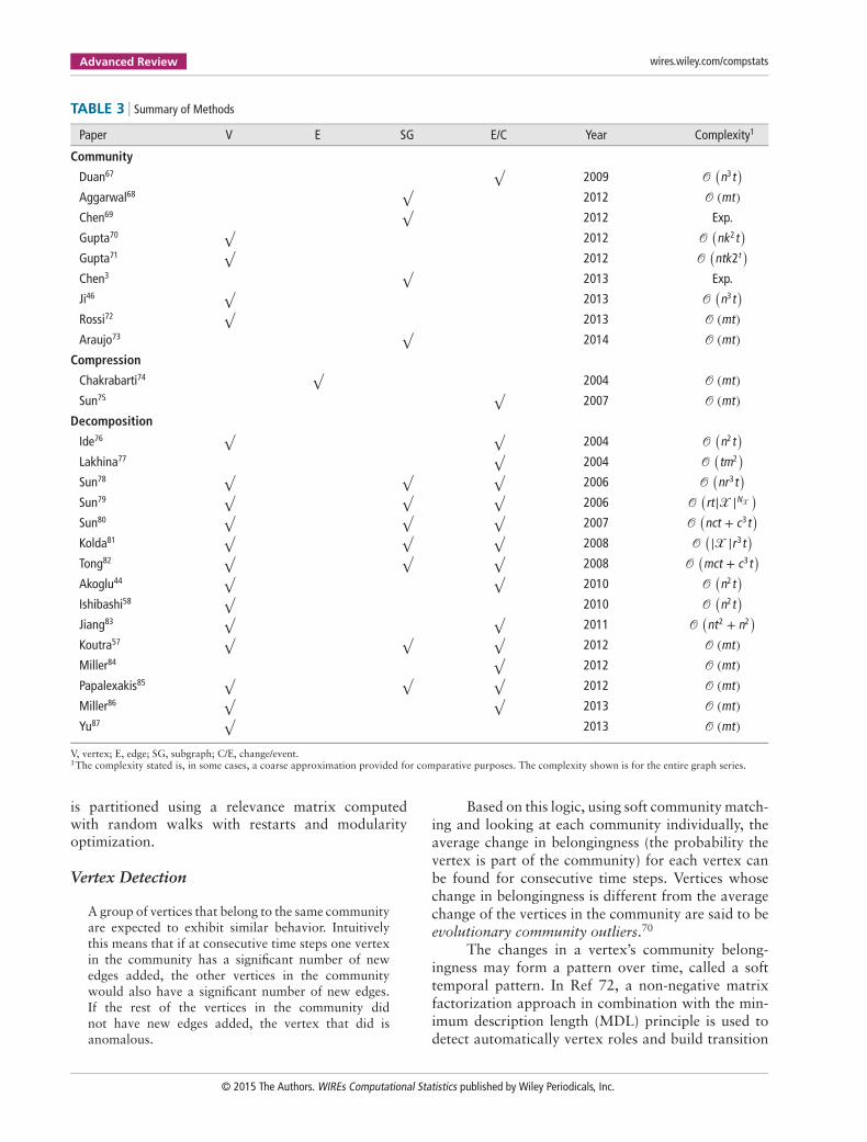
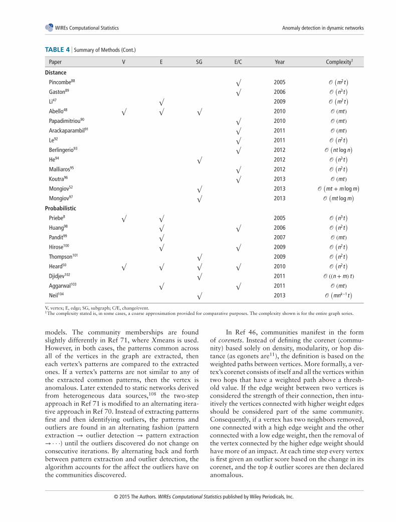
numbers, then applying existing anomaly detectors toidentify the anomalies. Equivalently, they are propos-ing methodologies for stage one, and applying existingmethodologies for stage two. A complete list of themethods surveyed is provided in Tables 3 and 4, withthe complexity notation provided in Table 5.
Community DetectionCommunity-based methods track the evolution ofcommunities and their associated vertices in thegraphs over time.105–107 While the data-specific fea-tures generated by the methods discussed in thissection are all derived using the community struc-ture of the graphs, the various approaches differ intwo main points: (1) in the aspects of the communitystructure they analyze, e.g., the connectivity withineach community versus how the individual vertices areassigned to the communities at each time step, and (2)in the definitions of communities they use, e.g., softcommunities where each vertex has a probability ofbelonging to each community versus disjoint commu-nities where each vertex is placed into at most onecommunity in the graph. Moreover, based on how thecommunity evolution is viewed, it can be applied tothe detection of different anomaly types. For example,a rapid expansion or contraction of a communitycould indicate that the specific subgraph for that com-munity is undergoing drastic changes, whereas a dropin the number of communities by two corresponds toan abnormal event.
ExampleIn Ref 67, given a weighted directed graph series G anda vertex partitioning similarity function Sim(Is, It), theset of change points is defined as a set of time pointsT : {t∈T|Sim(Is, It)≤ c0}. The similarity function isdefined as
Sim(Is, It
)=
PIs
(It
)+ PIt
(Is
)2N
, (1)
where PIs
(It
)=∑
p maxc∈Is∩It
|||Isp∩ c|||, Is is the partition-
ing of the current graph segment Gs and It is thepartitioning of the newly arrived graph Gt, N is thenumber of vertices, p is the community index in apartitioning, c is the common community betweenthe two partitionings. Mapping the similarity of twographs to a single score via vertex partition similar-ity is the extraction of the data-specific feature, andthe anomaly detector is the application of a thresholdvalue. If the similarity is above a threshold c0, then Gtwill be put into the current graph segment Gs, other-wise, Gt starts a new graph segment Gs+1. The graph
© 2015 The Authors. WIREs Computational Statistics published by Wiley Periodicals, Inc.
Advanced Review wires.wiley.com/compstats
TABLE 3 Summary of Methods
Paper V E SG E/C Year Complexity1
Community
Duan67√
2009 𝒪(n3t
)Aggarwal68
√2012 𝒪 (mt)
Chen69√
2012 Exp.
Gupta70√
2012 𝒪(nk2t
)Gupta71
√2012 𝒪
(ntk2t
)Chen3
√2013 Exp.
Ji46√
2013 𝒪(n3t
)Rossi72
√2013 𝒪 (mt)
Araujo73√
2014 𝒪 (mt)Compression
Chakrabarti74√
2004 𝒪 (mt)Sun75
√2007 𝒪 (mt)
Decomposition
Ide76√ √
2004 𝒪(n2t
)Lakhina77
√2004 𝒪
(tm2
)Sun78
√ √ √2006 𝒪
(nr3t
)Sun79
√ √ √2006 𝒪
(rt|𝒳 |N𝒳
)Sun80
√ √ √2007 𝒪
(nct + c3t
)Kolda81
√ √ √2008 𝒪
(|𝒳 |r3t)
Tong82√ √ √
2008 𝒪(mct + c3t
)Akoglu44
√ √2010 𝒪
(n2t
)Ishibashi58
√2010 𝒪
(n2t
)Jiang83
√ √2011 𝒪
(nt2 + n2
)Koutra57
√ √ √2012 𝒪 (mt)
Miller84√
2012 𝒪 (mt)Papalexakis85
√ √ √2012 𝒪 (mt)
Miller86√ √
2013 𝒪 (mt)Yu87
√2013 𝒪 (mt)
V, vertex; E, edge; SG, subgraph; C/E, change/event.1The complexity stated is, in some cases, a coarse approximation provided for comparative purposes. The complexity shown is for the entire graph series.
is partitioned using a relevance matrix computedwith random walks with restarts and modularityoptimization.
Vertex Detection
A group of vertices that belong to the same communityare expected to exhibit similar behavior. Intuitivelythis means that if at consecutive time steps one vertexin the community has a significant number of newedges added, the other vertices in the communitywould also have a significant number of new edges.If the rest of the vertices in the community didnot have new edges added, the vertex that did isanomalous.
Based on this logic, using soft community match-ing and looking at each community individually, theaverage change in belongingness (the probability thevertex is part of the community) for each vertex canbe found for consecutive time steps. Vertices whosechange in belongingness is different from the averagechange of the vertices in the community are said to beevolutionary community outliers.70
The changes in a vertex’s community belong-ingness may form a pattern over time, called a softtemporal pattern. In Ref 72, a non-negative matrixfactorization approach in combination with the min-imum description length (MDL) principle is used todetect automatically vertex roles and build transition
© 2015 The Authors. WIREs Computational Statistics published by Wiley Periodicals, Inc.
WIREs Computational Statistics Anomaly detection in dynamic networks
TABLE 4 Summary of Methods (Cont.)
Paper V E SG E/C Year Complexity1
Distance
Pincombe88√
2005 𝒪(m2t
)Gaston89
√2006 𝒪
(n3t
)Li47
√2009 𝒪
(m2t
)Abello48
√ √ √2010 𝒪 (mt)
Papadimitriou90√
2010 𝒪 (mt)Arackaparambil91
√2011 𝒪 (mt)
Le92√
2011 𝒪(n2t
)Berlingerio93
√2012 𝒪
(nt log n
)He94
√2012 𝒪
(n3t
)Malliaros95
√2012 𝒪
(n2t
)Koutra96
√2013 𝒪 (mt)
Mongiov52√
2013 𝒪(mt + m log m
)Mongiov97
√2013 𝒪
(mt log m
)Probabilistic
Priebe8√ √
2005 𝒪(n3t
)Huang98
√ √2006 𝒪
(n2t
)Pandit99
√2007 𝒪 (mt)
Hirose100√ √
2009 𝒪(n2t
)Thompson101
√2009 𝒪
(n2t
)Heard50
√ √ √ √2010 𝒪
(n2t
)Djidjev102
√2011 𝒪 ((n + m) t)
Aggarwal103√ √
2011 𝒪 (mt)Neil104
√2013 𝒪
(mnk−1t
)V, vertex; E, edge; SG, subgraph; C/E, change/event.1The complexity stated is, in some cases, a coarse approximation provided for comparative purposes. The complexity shown is for the entire graph series.
models. The community memberships are foundslightly differently in Ref 71, where Xmeans is used.However, in both cases, the patterns common acrossall of the vertices in the graph are extracted, theneach vertex’s patterns are compared to the extractedones. If a vertex’s patterns are not similar to any ofthe extracted common patterns, then the vertex isanomalous. Later extended to static networks derivedfrom heterogeneous data sources,108 the two-stepapproach in Ref 71 is modified to an alternating itera-tive approach in Ref 70. Instead of extracting patternsfirst and then identifying outliers, the patterns andoutliers are found in an alternating fashion (patternextraction → outlier detection → pattern extraction→ · · ·) until the outliers discovered do not change onconsecutive iterations. By alternating back and forthbetween pattern extraction and outlier detection, thealgorithm accounts for the affect the outliers have onthe communities discovered.
In Ref 46, communities manifest in the formof corenets. Instead of defining the corenet (commu-nity) based solely on density, modularity, or hop dis-tance (as egonets are11), the definition is based on theweighted paths between vertices. More formally, a ver-tex’s corenet consists of itself and all the vertices withintwo hops that have a weighted path above a thresh-old value. If the edge weight between two vertices isconsidered the strength of their connection, then intu-itively the vertices connected with higher weight edgesshould be considered part of the same community.Consequently, if a vertex has two neighbors removed,one connected with a high edge weight and the otherconnected with a low edge weight, then the removal ofthe vertex connected by the higher edge weight shouldhave more of an impact. At each time step every vertexis first given an outlier score based on the change in itscorenet, and the top k outlier scores are then declaredanomalous.
© 2015 The Authors. WIREs Computational Statistics published by Wiley Periodicals, Inc.
Advanced Review wires.wiley.com/compstats
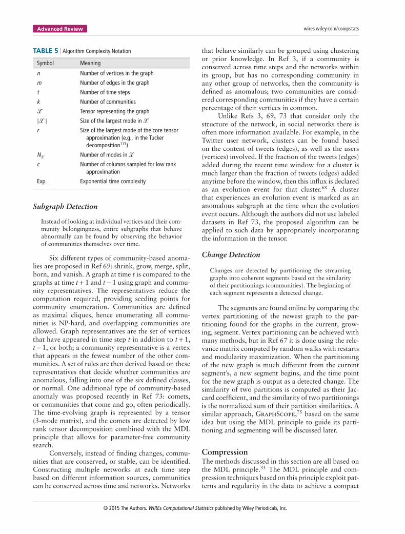
TABLE 5 Algorithm Complexity Notation
Symbol Meaning
n Number of vertices in the graph
m Number of edges in the graph
t Number of time steps
k Number of communities
𝒳 Tensor representing the graph
|𝒳 | Size of the largest mode in 𝒳
r Size of the largest mode of the core tensorapproximation (e.g., in the Tuckerdecomposition113)
N𝒳 Number of modes in 𝒳
c Number of columns sampled for low rankapproximation
Exp. Exponential time complexity
Subgraph Detection
Instead of looking at individual vertices and their com-munity belongingness, entire subgraphs that behaveabnormally can be found by observing the behaviorof communities themselves over time.
Six different types of community-based anoma-lies are proposed in Ref 69: shrink, grow, merge, split,born, and vanish. A graph at time t is compared to thegraphs at time t+ 1 and t− 1 using graph and commu-nity representatives. The representatives reduce thecomputation required, providing seeding points forcommunity enumeration. Communities are definedas maximal cliques, hence enumerating all commu-nities is NP-hard, and overlapping communities areallowed. Graph representatives are the set of verticesthat have appeared in time step t in addition to t+1,t−1, or both; a community representative is a vertexthat appears in the fewest number of the other com-munities. A set of rules are then derived based on theserepresentatives that decide whether communities areanomalous, falling into one of the six defined classes,or normal. One additional type of community-basedanomaly was proposed recently in Ref 73: comets,or communities that come and go, often periodically.The time-evolving graph is represented by a tensor(3-mode matrix), and the comets are detected by lowrank tensor decomposition combined with the MDLprinciple that allows for parameter-free communitysearch.
Conversely, instead of finding changes, commu-nities that are conserved, or stable, can be identified.Constructing multiple networks at each time stepbased on different information sources, communitiescan be conserved across time and networks. Networks
that behave similarly can be grouped using clusteringor prior knowledge. In Ref 3, if a community isconserved across time steps and the networks withinits group, but has no corresponding community inany other group of networks, then the community isdefined as anomalous; two communities are consid-ered corresponding communities if they have a certainpercentage of their vertices in common.
Unlike Refs 3, 69, 73 that consider only thestructure of the network, in social networks there isoften more information available. For example, in theTwitter user network, clusters can be found basedon the content of tweets (edges), as well as the users(vertices) involved. If the fraction of the tweets (edges)added during the recent time window for a cluster ismuch larger than the fraction of tweets (edges) addedanytime before the window, then this influx is declaredas an evolution event for that cluster.68 A clusterthat experiences an evolution event is marked as ananomalous subgraph at the time when the evolutionevent occurs. Although the authors did not use labeleddatasets in Ref 73, the proposed algorithm can beapplied to such data by appropriately incorporatingthe information in the tensor.
Change Detection
Changes are detected by partitioning the streaminggraphs into coherent segments based on the similarityof their partitionings (communities). The beginning ofeach segment represents a detected change.
The segments are found online by comparing thevertex partitioning of the newest graph to the par-titioning found for the graphs in the current, grow-ing, segment. Vertex partitioning can be achieved withmany methods, but in Ref 67 it is done using the rele-vance matrix computed by random walks with restartsand modularity maximization. When the partitioningof the new graph is much different from the currentsegment’s, a new segment begins, and the time pointfor the new graph is output as a detected change. Thesimilarity of two partitions is computed as their Jac-card coefficient, and the similarity of two partitioningsis the normalized sum of their partition similarities. Asimilar approach, GraphScope,75 based on the sameidea but using the MDL principle to guide its parti-tioning and segmenting will be discussed later.
CompressionThe methods discussed in this section are all based onthe MDL principle.33 The MDL principle and com-pression techniques based on this principle exploit pat-terns and regularity in the data to achieve a compact
© 2015 The Authors. WIREs Computational Statistics published by Wiley Periodicals, Inc.
WIREs Computational Statistics Anomaly detection in dynamic networks
graph representation.109 Applying this principle tographs is done by viewing the adjacency matrix ofa graph as a single binary string, flattened in rowor column major order. If the rows and columns ofthe matrix can be rearranged such that the entropyof the binary string representation of the matrix isminimized, then the compression cost (also known asencoding cost34) is minimized. The data-specific fea-tures are all derived from the encoding cost of thegraph or its specific substructures; hence, anomaliesare then defined as graphs or substructures (e.g., edges)that inhibit compressibility.
ExampleIn Ref 75, given unweighted and undirected graphseries G and segment encoding cost function c, theset of change points is defined as a set of time pointsT ∶
{t ∈ T|c (Gs ∪
{Gt
})− c
(Gs)
≥ c(Gt
)}, where
Gs is the current graph segment, and Gt is the newlyarrived graph at time point t. The main differencebetween GraphScope75 and the example from theCommunity Detection section by Duan et al67 is thescoring function used for partitioning and changedetection. Equivalently, the two methods generate dif-ferent data-specific features. Duan et al.67 used com-munity driven metrics, computed by random walkswith restarts and modularity optimization, to parti-tion and segment the graphs, whereas, GraphScope75
is guided by the MDL principle, using encoding cost asa scoring function. While both methods use a thresh-old system as an anomaly detector, GraphScopeuses a dynamic threshold, based on the current graphsegment, instead of a fixed threshold as in Ref 67.
Edge Detection
An edge is considered anomalous if the compressionof a subgraph has higher encoding cost when the edgeis included than when it is omitted.
In Ref 74, a two-step alternating iterativemethod is used for automatic partitioning of the ver-tices. Vertex partitioning can be done by rearrangingthe rows and columns in the adjacency matrix. Inthe first step, the vertices are separated into a fixednumber of disjoint partitions such that the encodingcost is minimized. The second step iteratively splitsthe partitions with high entropy into two. Any vertexwhose removal from the original partition wouldresult in a decrease in entropy is removed from thatpartition and placed into the new one. Once themethod has converged, meaning steps 1 and 2 areunable to find an improvement, the edges can begiven outlierness scores. The score for each edge iscomputed by comparing the encoding cost of the
matrix including the edge to the encoding cost if theedge is removed. Streaming updates can be performedusing the previous result as a seed for a new run ofthe algorithm, thus avoiding full recomputations.
Change Detection
The main idea is that consecutive time steps that arevery similar can be grouped together leading to lowcompression cost. Increases in the compression costmean that the new time step differs significantly fromthe previous ones, and thus signifies a change.
Akin to Ref 67, to detect changes in a graphstream, consecutive time steps that are similar can begrouped into segments. When considering the nextgraph in the stream, it can either be grouped withthe graphs in the current segment, or it can be thebeginning of a new segment. The decision to start anew segment in Ref 75 is made by comparing theencoding cost of the current segment without the nextgraph to the encoding cost of the segment if the nextgraph were included. If the vertex partitioning for thenew graph is very similar to the vertex partitioning ofthe graphs in the segment then the encoding cost willnot change much. However, if the partitions are verydifferent, the encoding cost would increase because ofthe increase in entropy. Changes in the graph streamare the time points when a new segment begins. Thismethod is also parameter-free.
Matrix/Tensor DecompositionThese techniques represent the set of graphs as atensor, most easily thought of as a multidimensionalarray, and perform tensor factorization or dimen-sionality reduction. The most straightforward methodfor modeling a dynamic graph as a tensor is to cre-ate a dimension for each graph aspect of interest,e.g., a dimension for time, source vertices, and des-tination vertices. For example, modeling the Enronemail dataset can be done using a 4-mode tensor, withdimensions for sender, recipient, keyword, and date.The element (i, j, k, l) is 1 if there exists an email thatis sent from sender i to recipient j with keyword k onday l, otherwise, it is 0.
Similar to compression techniques, decomposi-tion techniques search for patterns or regularity inthe data to exploit. All of the data-specific featuresgenerated by these methods are derived from theresult of the decomposition of a matrix or tensor.Unlike the community methods, these typically takea more global view of the graphs, but are able toincorporate more information (attributes) via addi-tional dimensions in a tensor. One of the most popular
© 2015 The Authors. WIREs Computational Statistics published by Wiley Periodicals, Inc.
Advanced Review wires.wiley.com/compstats
methods for matrices (2-mode tensors) is singularvalue decomposition (SVD),37 and for higher ordertensors (≥3 modes) is PARAFAC,110 a generalizationof SVD. The main differences among the decomposi-tion based methods are whether they use a matrix ora higher order tensor, how the tensor is constructed(what information is stored), and the method ofdecomposition.
ExampleIn Ref 44, given the 3-D T ×N×F tensor, whereT denotes the number of time steps, N denotes thenumber of vertices in a graph, F denotes the num-ber of features extracted for each vertex, a scoringfunction Z(t), and the time window W, a set of timepoints for change detection is a set of time stepsT
′: {t∈T
′|Z(t)≥ c0}, where c0 is a dynamic threshold,
Z(t)= 1− u(t)Tr(t− 1), u(t) is the principal Eigen-vector (or ‘Eigen-behavior’) of the vertex-to-vertexfeature correlation matrix computed at time point t,and r(t− 1) is the ‘typical Eigen-behavior’, calculatedusing the last W Eigenvectors. Each time points score,Z(t), can be thought of as the similarity between thecurrent graph, and the previous W graphs. Using theZ scores that are output as the data-specific features,the anomaly detector is a simple heuristic of choosingthe top k values and labeling them as the anomalies.Similar to the examples in the Community Detectionand Compression-based sections, this method incor-porates the historical values into the data-specificfeature generation instead of the anomaly detector.However, unlike the previous two examples, it con-siders the entire graph at once to compute its score,instead of building up the score based on substruc-tures or partitions, and uses a fixed sliding windowof graphs over the time series instead of a dynamicsegmenting process.
Vertex Detection
Matrix decomposition is used to obtain activity vec-tors per vertex. A vertex is characterized as anomalousif its activity changes significantly between consecutivetime steps.
Owing to the computational complexity of per-forming principal component analysis111 (PCA) on theentire graph, it is computationally advantageous toapply it locally. The approach used in Ref 87 is tohave each vertex maintain an edge correlation matrixM, which has one row and column for every neigh-bor of the vertex. The value of an entry in the matrixfor vertex i, M(j, k), is the correlation between theweighted frequencies of the edges (i, j) and (i, k). The
weighted frequencies are found using a decay function,where edges that occurred more recently have a higherweight. The largest Eigenvalue and its correspondingvector obtained by performing PCA on M are sum-maries of the activity of the vertex and the correlationof its edges, respectively. The time series formed byfinding the changes in these values are used to com-pute a score for each vertex at each time step. Verticesthat have a score above a threshold value are outputas anomalies at that time.
Event Detection
There are two main approaches: (1) Tensor decom-position approximates the original data in a reduceddimensionality, and the reconstruction error is an indi-cator of how well the original data is approximated.Sub-tensors, slices, or individual fibers in the tensorthat have high reconstruction error do not exhibitbehavior typical of the surrounding data, and revealanomalous vertices, subgraphs, or events. (2) Singularvalues and vectors, as well as Eigenvalues and Eigen-vectors are tracked over time in order to detect signif-icant changes that showcase anomalous vertices.
Using the reconstruction error as an indicatorfor anomalies has been employed for detecting timesduring molecular dynamics simulations where thecollective motions suddenly change,54 finding framesin a video that are unlike the others,56 and identifyingdata that do not fit any concepts.112
To address the intermediate blowup problem—when the input tensor and output tensors exceedmemory capacity during the computation—memory-efficient tucker (MET) decompositionwas proposed,81 based on the original Tuckerdecomposition.113 The Tucker decomposition approx-imates a higher order tensor using a smaller core tensor(thought of as a compressed version of the originaltensor) and a matrix for every mode (dimension)of the original tensor. Similarly, methods have beendeveloped for offline, dynamic, and streaming tensoranalysis,79 in addition to static and sliding windowbased methods.78 These extensions allow the methodto operate on continuous graph streams as well asthose with a fixed number of time points. Compactmatrix decomposition80 (CMD) computes a sparselow rank approximation of a given matrix. By apply-ing CMD to every adjacency matrix in the stream,a time series of reconstruction values is created andused for event detection. Colibri82 and ParCube85
can be used in the same fashion and provide a largeincrease in efficiency. The PARAFAC decompositionhas been shown to be effective at spotting anomaliesin tensors as well.57
© 2015 The Authors. WIREs Computational Statistics published by Wiley Periodicals, Inc.
WIREs Computational Statistics Anomaly detection in dynamic networks
Instead of finding the difference between thegraph reconstructed from the approximation obtainedby a decomposition, a probabilistic model can be used.The Chung-Lu random graph model114 is used inRef 84 Taking the difference between the real graph’sadjacency matrix and the expected graph’s forms aresidual matrix. Anomalous time windows are foundby performing SVD on the residual matrices—onwhich a linear ramp filter has been applied—andby analyzing the change in the top singular values.The responsible vertices are identified via inspectionof the right singular vectors. More accurate graphmodels that also consider attributes are proposedin Ref 86.
Going away from comparing an expected orapproximate model of the graph to the real model tofind the deviation, events can be identified via signifi-cant changes in the decomposed space. Specifically, byperforming PCA on the data, the calculated Eigenvec-tors can be separated into ‘normal’ and ‘anomalous’sets by examining the values of the data projected ontoeach Eigenvector. At each time step the Eigenvectorsare examined (via projection of the data) in descend-ing order of their corresponding Eigenvalues, and thefirst Eigenvector to contain a projected point outside 3standard deviations of the rest of the values, and everyEigenvector thereafter, constitute the anomalous set.The second step is then to project the data onto itsnormal and anomalous subspaces. Once this is done,events are detected when the modifications in theanomalous components from the previous time step tothe current are above a threshold value.77 Expandingon this method, joint sparse PCA and graph-guidedjoint sparse PCA were developed to localize theanomalies and identify the vertices responsible.83 Theresponsible vertices are more easily identified by usinga sparse set of components for the anomalous set. Ver-tices are given an anomaly score based on the valuesof their corresponding row in the abnormal subspace.As a result of the anomalous components being sparse,the vertices that are not anomalous receive a score of0. Owing to the popularity of PCA in traffic anomalydetection, a study was performed identifying and eval-uating the main challenges of using PCA.115
Change Detection
The activity vector of a graph, u(t), is the principalcomponent, the left singular vector corresponding tothe largest singular value obtained by performing SVDon the weighted adjacency matrix. A change point iswhen an activity vector is substantially different fromthe ‘normal activity’ vector, which is derived fromprevious activity vectors.
The normal activity vector, r(t− 1), is the leftsingular vector obtained by performing SVD on thematrix formed by the activity vectors for the lastW time steps. Each time point is given a scoreZ(t)= 1− r(t−1)Tu(t), which is intuitively a score ofhow different the current activity is compared tonormal, where a higher value is worse. Anomalies canbe found online using a dynamic thresholding scheme,where time points with a score above the thresholdare output as changes.76 The vertices responsible arefound by calculating the ratio of change betweenthe normal and activity vectors. The vertices thatcorrespond to the indexes with the largest change arelabeled anomalous. Similar approaches have used theactivity vector of a vertex-to-vertex feature correlationmatrix,44 and a vertex-to-vertex correlation matrixbased on the similarity between vertex’s neighbors.58
Distance MeasuresUsing the notion of distance as a metric to measurechange is natural and widely used.23,60,116,117 Twoobjects that have a small difference in a measuredmetric can be said to be similar. The metrics measuredin graphs are typically structural features, such asthe number of vertices. Once the summary metricsare found for each graph, the difference or similarity,which are inversely related, can be calculated. Thevariation in the algorithms lies in the metrics chosento extract and compare, and the methods they use todetermine the anomalous values and correspondinggraphs.
ExampleIn Ref 96, given a graph series G, a distance functiond that computes the distance between two matrices,and a function to calculate the vertex affinity matrixS, where sij indicates the influence vertex i has onvertex j, a set of time points for detected events isT : {t∈T|d(Gt, Gt+1)≤ c0}, where
d(Gt ,Gt +1
)=
√√√√ n∑i=1
n∑j=1
(√St,ij −
√St+1,ij
)2, (2)
and c0 is a threshold value. Similar to the examplegiven in the Community Detection section,67 thedata-specific feature of interest here is a measure offinding the distance (inversely related to similarity)between two graphs. Thus, each adjacent graph pairis mapped to a single real value, creating a timeseries. The anomaly detector, the quality control mov-ing average threshold, is unique compared to theprevious examples, as it considers the historical val-ues of the data-specific features. The previous three
© 2015 The Authors. WIREs Computational Statistics published by Wiley Periodicals, Inc.
Advanced Review wires.wiley.com/compstats
sections (Community Detection, Compression, andDecomposition) incorporated this information intotheir data-specific feature generation, using window-ing or segmenting techniques.
Edge Detection
If the evolution of some edge attribute (e.g., edgeweight) differs from the ‘normal’ evolution, then thecorresponding edge is characterized as anomalous.
In Ref 47, a dynamic road traffic network whoseedge weights vary over time is studied. The similaritybetween the edges over time is computed using a decayfunction that weighs the more recent patterns higher.At each time step, an outlierness score is calculatedfor each edge based on the sum of the changes insimilarity scores. Edges with the highest score, chosenusing either a threshold value or top-k heuristic, aremarked as anomalous at that time step.
Viewing the network as a stream of edges,meaning the network does not have a fixed topologyas the road traffic network did, the frequency andpersistence of an edge can be measured and used asan indicator of its novelty. The persistence of an edgeis how long it remains in the graph once it is added,and the frequency is how often it appears. In Ref 48,set system discrepancy118 is used to measure thepersistence and frequency of the edges. When an edgearrives, its discrepancy is calculated and compared tothe mean discrepancy value of the active edge set. Ifthe weighted discrepancy of the edge is more than athreshold level greater than the mean discrepancy, theedge is declared novel (anomalous). Using the noveledges detected, a number of metrics can be calculatedfor various graph elements (e.g., vertices, edges, andsubgraphs). Individual graph elements can then beidentified anomalous via comparison of the calculatedmetrics for that element with the overall distributionand change of the metric.
Subgraph Detection
A subgraph with many ‘anomalous’ edges is deemedanomalous.
Contrasting with Ref 46 where the edge weightsare considered the strength of a connection, in Ref52 the edge weights are considered as outlier scores,or how ‘anomalous’ that edge is at that time. Everyedge at every time step is given its own anomaly score,which is a function of the probability of seeing thatparticular edge weight on that particular edge giventhe distribution of weights for that edge over all thegraphs in the series. Alternatively, the output of an
existing method that assigns outlier scores for edgesin a network47,48,50,74,119 could be used as the inputto this method. The latter approach allows52 to beapplied to any network that is capable of having out-lier scores assigned to edges (e.g., weighted, directed,and attributed). Once every edge is assigned an outlierscore, significant anomalous regions (SARs)—fixedsubgraphs over a window of time—are mined fromthe sequence, analogous to the problem of finding theHDSs. An alternating iterative approach based on Ref120—first finding an optimal time window for a fixedsubgraph, then finding an optimal subgraph for thefixed time window, repeating until no improvementis found—is constructed to approximate a solution tothe NP-hard problem. This work was later extendedto allow the subgraphs to smoothly evolve over time,where vertices can be added or removed between adja-cent time steps.97 A similar approach mines weightedfrequent subgraphs in network traffic, where the edgeweights correspond to the anomaly contribution ofthat edge.94
Event Detection
Provided a function f (Gi, Gj) that measures the dis-tance between two graphs, a time series of distancevalues can be constructed by applying the function onconsecutive time steps in the series. Anomalous val-ues can then be extracted from this time series usinga number of different heuristics, such as selecting thetop k or using a moving average threshold.
Extracting features from the graphs is a commontechnique to create a summary of the graph in a fewscalar values, its signature. Local features are specificto a single vertex and its egonet11 (the subgraphinduced by itself and its one-hop neighbors), suchas the vertex or egonet degree. Global features arederived from the graph as a whole, such as thegraph radius. The local features of every vertex inthe graph can be agglomerated into a single vector,the signature vector, of values that describe the graphusing the moments of distribution (such as meanand standard deviation) of the feature values. InRef 93, the similarity between two graphs is theCanberra distance, a weighted version of the L1distance, between the two signature vectors. A similarapproach is used in Ref 92 to detect abnormal times intraffic dispersion graphs. Instead of an agglomerationof local features, it extracts global features from eachgraph, introducing a dK-2 series121–123-based distancemetric, and any graph with a feature value above athreshold is anomalous.
As an alternative to extracting multiple featuresfrom the graph and using the signatures, the pairwise
© 2015 The Authors. WIREs Computational Statistics published by Wiley Periodicals, Inc.
WIREs Computational Statistics Anomaly detection in dynamic networks
vertex affinity scores may be used. Pairwise vertexaffinity scores are a measure of how much each vertexinfluences another vertex, and can be found using fastbelief propagation.124 In Ref 96, the scores are calcu-lated for two consecutive time steps, and the similaritybetween the two graphs is the rooted Euclidean dis-tance (Matusita distance) between the score matrices.The changes in the vertex affinity score are shown toaccurately reflect and scale with the level of impactof the changes. For example, removing an edge thatconnects two otherwise disconnected components, a‘bridging edge’, results in a higher score than remov-ing an edge that does not affect the overall structureof the graph. A moving threshold is set on the timeseries of similarity scores using quality control withindividual moving range. The exponential weightedmoving average has also been used as a way todynamically set the threshold, tested on distributionfeatures extracted from Wikipedia revision logs.91
Complementary to feature similarity, one canlook at the structural differences between graphsto identify the magnitude of change. These meth-ods focus on the function that defines the distancebetween graphs instead of finding the optimal featuresto use as summaries. Many metrics have been devel-oped and tested to quantify the differences betweengraphs. In Ref 88, 10 different distance functionswere evaluated on TCP/IP traffic graphs with knownanomalies (ground truth). Box-Jenkins autoregressivemoving average (ARMA) modeling125 was used tocreate a ‘normal’ model of the feature values, andthe time points with residuals, calculated as the dif-ference between expected and real value, exceedinga threshold are flagged. The 10 distance functionstested were weight, maximum common subgraph(MCS) weight, MCS edge, MCS vertex, graph editdistance, median graph edit distance, modality, diam-eter, entropy, and spectral. Of these 10 distance func-tions, the MCS-based methods performed the best;however, finding the MCS between two graphs is anNP-hard problem. More recently in Ref 90, five dif-ferent distance scoring functions, all with a linearcomplexity, were tested on web graphs with specifictypes of anomalies: missing subgraph, missing vertices,and connectivity change. The five scoring functionswere: vertex/edge overlap, vertex ranking, vector sim-ilarity, sequence similarity, and signature similarity.The method that performed the best was the signa-ture similarity, which is done by extracting a signa-ture vector from each graph and finding the distancebetween them using SimHash.126 Unlike the signa-ture vectors discussed above that create summaries ofthe entire graph in a few scalar values, the signaturehere includes every vertex and edge. Specifically, the
features used were each vertex and its PageRankvalue, and each edge (u, v) with a weight equal to u’sPageRank value divided by the number of outlinksfrom u. Weighting the vertices with their ‘quality’,measured by PageRank, ensures that the removal of ahigh-quality vertex will have more of an impact thanthe removal of a low quality vertex. A fixed thresholdwas set to find graphs with abnormally low similarityscores.
Instead of finding structural difference betweentwo consecutive graphs, events can be detected usingthe time series of robustness values for each graph.Robustness is a measure of the connectivity of thegraph. A graph with a high robustness will retain thesame general structure and connectivity even whensome vertices or edges are removed. Finding eventsis then finding when the robustness value changessignificantly.95 A similar approach is given in Ref 89,but using a variant of the graph diameter. The graphdiameter used is the average of all vertex eccentricities(the eccentricity of a vertex v is the longest shortestpath from v to any other vertex), instead of the typicaldefinition of using the maximum vertex eccentricity.Both the time series of graph diameter changes and thegraph diameters themselves are shown to be effectivemethods for detecting events.
Probabilistic ModelsWith a foundation in probability theory, distributions,and scan statistics, these methods typically constructa model of what is considered ‘normal’ or expected,and flag deviations from this model as anomalous. Thetype of model used, how it is constructed, what it ismodeling, and the method for determining outliers iswhat differentiates these approaches.
ExampleIn Ref 98, given a graph series G and a likelihood scor-ing function L, a set of time points for change detec-tion is a set of time steps T : {t∈T|log(L(t))/|𝜃|≤ c0},where L(t)=
∏𝜃appear in time t P(𝜃)c(𝜃), 𝜃 denotes
sender–recipient tuples, P(𝜃) indicates the probabilityof all possible sender–recipient tuples (emails from asingle sender to a list of receivers), and c(𝜃) is the num-ber of occurrences of a particular sender–recipienttuple in time t. Thus, each time step is mapped toa single value, the average log-likelihood, indicatingthe predictability of the emails during that time step,high values indicating normal behavior. Abnormaltime steps are identified via inspection of the plotof log-likelihood values. In general, the data-specificfeatures that are output are often probabilities, orlikelihoods, of certain structures or events occurring.
© 2015 The Authors. WIREs Computational Statistics published by Wiley Periodicals, Inc.
Advanced Review wires.wiley.com/compstats
Typically, models or distributions are constructedusing past data to derive an ‘expected’ case for thenext time step. Anomaly detectors in probabilisticmethods do not always perform a hard mappingfrom features to anomalies, where everything is eithernormal or abnormal, but can provide a probabilitythat the structure or event is anomalous.
Vertex Detection
There are two main approaches: (1) Building scanstatistics time series and detecting points that areseveral standard deviations away from the mean, (2)vertex classification.
Scan statistics are often called ‘moving windowanalysis’, where the local maximum or minimum of ameasured statistic is found in specific regions of thedata. In a graph, a scan statistic can be consideredas the maximum of a graph invariant feature, suchas the number of edges, found for each vertex andits neighborhood in the graph. In Ref 8, they use avariable ‘scale’ for the measured statistic; each vertexhas the number of edges in its 0, 1, and 2 stepneighborhood measured. The local statistic for eachvertex is then normalized using the mean and standarddeviation of its recent values, and the scan statisticof a graph is the maximum of all of the normalizedlocal statistics. Normalizing the values accounts forthe history of each vertex, meaning the statistic foreach vertex is relative to its own past instead ofthe values of the other vertices. This ensures thatthe largest change measured in the graph is not tieddirectly to the magnitude of change, but the ratio.Building a standardized time series of the scan statisticvalues, any value that is five standard deviations awayfrom the mean of the series is considered an event(hence, events are detected as well). The vertex mostresponsible is identified as the one that was chosen forthe scan statistic value for the entire graph.
Similar to the use of neighborhoods for scanstatistics, the Markov random field model (MRF) isused to uncover the states for vertices and infer themaximum likelihood assignment by a belief propaga-tion algorithm, where a vertex is labeled based on thevertices it is connected to. In Ref 99, anomalies (fraud-sters) are uncovered in an online auction network bydiscovering bipartite cores, which are posited to be theinteraction behavior between fraudsters and accom-plices. It incrementally updates the model as new edgesare added, taking advantage of the fact that an edgeinsertion or removal will affect only a local subgraph.In the propagation matrix a vertex can be in one ofthree states: fraudster, accomplice, or honest. Verticesthat are assigned the label of fraudster are anomalous.
Edge Detection
Communications (edges) are modeled using a count-ing process, and edges that deviate from the model bya statistically significant amount are flagged.
One way to model the relationship between ver-tices is considering the communication between themas a counting process. In Ref 50, a Bayesian discretetime counting process is used to model the number ofcommunications (edge weights) between vertices, andis continuously updated as new graphs are considered.Predictive p-values, based on the learning of the dis-tribution of the counts, are calculated for the edges ofthe newest observation and subsequently used for flag-ging anomalous vertex pairs (edges). Moreover, as newgraphs are considered, both sequential—comparingthe new graph to the model based on history—andretrospective analysis—adjusting the history based onthe newest graphs—are performed. The retrospectiveanalysis helps alleviate the insufficient data problem,when decisions are made early on with insufficient his-tory to be accurate.
Subgraph Detection
Fixed subgraphs (e.g., paths and stars), multigraphs,and cumulative graphs are used to construct models onthe expected behaviors. Deviations from the modelssignify an anomalous subgraph.
To identify hacker behaviors in a network,104
combines scan statistics with a Hidden Markov Model(HMM) for edge behavior. Unlike Ref 8 that usedneighborhoods, the local scan statistics are based ontwo graph shapes, the k-path and star. Comparingthe scan statistics of a sliding window to its pastvalues, and using an online thresholding system, localanomalies are identified. The local anomaly is theunion of all subgraphs (representing the k-paths orstars) that led to statistically significant test statistics.
Another method to model a dynamic network,instead of using a series or stream of graphs, is to havea single multigraph where parallel edges correspond tocommunication between vertices at two different timesteps. The initial multigraph is decomposed into tele-scoping subgraphs (TSGs) for each time window.102
A TSG satisfies two conditions: (1) for any two edgesthat share a vertex, the edge that begins communica-tion first finishes communication last; (2) there exists avertex r, the root, that has no incoming edges and has apath to every vertex in the TSG. TSGs that have a lowprobability of appearing (according to their size andhistoric connection patterns) are output as anomalies.
Likewise, a cumulative graph, which includesevery edge seen up until the current time step, is
© 2015 The Authors. WIREs Computational Statistics published by Wiley Periodicals, Inc.
WIREs Computational Statistics Anomaly detection in dynamic networks
used in Ref 101. Edge weights in the graph arecalculated using a decay function where more recentedges weigh more. A normal behavior for subgraphsis defined by identifying persistent patterns, herefound by constructing a graph where each edge isweighted by the fraction of time it is in the graph anditeratively extracting the heaviest weight connectedcomponents. As the cumulative graph evolves theextracted subgraphs are monitored, comparing theircurrent activity to the expected activity, which is basedon the recent behavior.
Event Detection
Deviations from the models of the graph likelihoodor the distribution of the Eigenvalues reveal when anevent occurs.
Recently, a new reservoir sampling method wasproposed in Ref 103 to maintain structural summariesof a graph stream. The online sampling method man-ages multiple distinct partitionings of the network toprovide a statistically significant summary. As a newgraph is added to the stream, every edge has its likeli-hood calculated based on the edge generation modelsof the different partitions. Once the edge likelihoodshave been found an global graph likelihood is calcu-lated as the geometric mean of the edge likelihoodvalues. A similar edge generation model approach wasused in Ref 98, where the probability that and edgeexists between vertices i and j is stored in a matrix,M(i, j). The estimated probabilities are calculatedusing expectation maximization, and subsequentlyused to give potential scores to every sender–recipientpair. Each sender–recipient tuple, which is an emailfrom one sender to multiple recipients, then has itslikelihood computed based on the estimated distribu-tion of all possible sender–recipient tuples. A singlescore is calculated for each graph as the average ofthe log-likelihood scores. In both of these methods asingle score is calculated for each graph based on thelikelihoods of the individual edges within it, and theindividual edges (or tuples) responsible are those thathave the lowest likelihood.
Similar to estimating the distribution of possiblesender–recipient tuples, the distribution of the Eigen-values and compressed Eigen equations is calculatedin Ref 100. Based on the assumption that each ver-tex has a time series of a vertex-local feature (e.g.,summed edge weight), a vertex-to-vertex correlationmatrix can be generated for each time step. The Eigenequation of the correlation matrix is compressed bykeeping the largest Eigenvalues and a set of low dimen-sion matrices (one matrix for each vertex). By learningthe distributions of the Eigenvalues and matrices, both
events and the vertices responsible can be identified.When the Eigenvalues deviate from the expected dis-tribution an event has occurred, and the vertices whosematrices deviate from the matrix distribution127 themost are considered responsible.100
DISCUSSION
With the wealth of algorithms discussed, the deci-sion of which to use can be difficult. The choicedepends on the types of graphs being analyzed (plain,attributed, directed, undirected, etc.), the desired typesof anomalies, and the size of the graphs—influencingthe allowed complexity, required parallelism, andwhether streaming analysis is required. It is worth not-ing, however, that using multiple methods in parallelor in conjunction with one another may yield superiorresults compared to using a single method. Using pub-licly available datasets (Table 7), each algorithm canbe applied to data from a variety of domains, com-paring the found anomalies, their sensitivity, and theirscalability.
While each method has its own advantages anddisadvantages, for brevity we will give an overviewof only those that have publicly available code (seeTable 6). We note that the available software listedis not comprehensive. We listed all software that wassaid to be available in their papers, as well as thesoftware of the authors that responded to our emailasking about the availability of their code. The meth-ods are again partitioned by the types of anomaliesthey detect so that a fair qualitative comparison canbe made. Note that a quantitative comparison amongthe available methods was impractical because themethods mostly detect different types of anomalies.Of the few intra-type comparisons that exist, coordi-nating the different outputs (e.g., anomalous verticesin the graphs versus anomalous vertices in communi-ties of the graphs) and attaining a valuable comparisonwould be unlikely.
Type 1 (Vertices) MethodsThe earliest work with available software is the onlinemethod by Heard et al.,50 which models the frequencyof the connections between vertices as a countingprocess and uses Bayesian learning and predictivep-values to identify anomalies.71,70,50 In addition tooperating on graph streams, it leverages the sparsityof the network by only examining edges that appearin the graphs. A key advantage of this technique isthat it performs both sequential analysis, where newgraphs are analyzed using the history of the graphstream, in addition to retrospective analysis, where
© 2015 The Authors. WIREs Computational Statistics published by Wiley Periodicals, Inc.
Advanced Review wires.wiley.com/compstats
TAB
LE6
Met
hods
with
Ope
nSo
urce
Code
,the
Type
sof
Gra
phs
they
Wor
kon
,the
Lang
uage
They
Are
Writ
ten
in,a
ndth
eO
utpu
tFor
mat
Code
Dire
cted
Und
irect
edW
eigh
ted
Unw
eigh
ted
Plai
nAt
trib
uted
Para
met
eriz
edSt
ream
ing
Lang
uage
Out
put
BAYE
SIAN
50√
√√
√√
√M
ATLA
B[0
,1]p
ertim
est
epan
d[0
,1]p
ered
gepe
rtim
est
ep
DELT
ACO
N96
√√
√√
√M
ATLA
B[0
,1]p
ertim
est
ep
NET
SPOT
52√
√√
√Ja
vaSu
bgra
phs
with
time
inte
rval
s
CTO
UTL
IER
711
√√
√√
√√
√Ja
va[0
,1]p
erve
rtex
fora
lltim
est
eps
ECO
UTL
IER70
1√
√√
√√
√√
√Ja
va[0
,1]p
erve
rtex
perc
omm
unity
per
time
step
PARC
UBE
85√
√√
√√
√√
√M
ATLA
BTe
nsor
fact
ors
fora
lltim
est
eps
1T
hese
met
hods
oper
ate
onth
eco
mm
unit
ybe
long
inge
ssm
atri
ces
ofgr
aphs
,the
refo
reth
eyar
eap
plic
able
toan
ygr
aph
that
can
have
com
mun
itie
sex
trac
ted.
the history is updated based on the new graphs thatarrive. One example of when this could be usefulis in the initial stages of the analysis when very lit-tle history is available. When the algorithm termi-nates the output is very easy to interpret, labeling ver-tices/edges/subgraphs explicitly as anomalous or not.The flexibility of the final part of the algorithm, whenanalysis is performed on only the identified anomalousportions of the graph and their neighbors, opens manypossibilities—anomalous community detection, iden-tifying the most important or influential anomalousvertex, and many more.
Similar to Ref 50, ECOutlier70 can be per-formed on graph streams. Each new graph will havea community detection algorithm run on it, and thenthe community matching and anomaly detection canbe performed. However, it compares only two adja-cent time points in the graph stream—the newly addedgraph and the one immediately preceding it. An inter-esting feature of this method is that it operates onthe community belongingness matrices of a graph,and is therefore applicable to graphs of any type(plain, attributed, directed, etc.). The output fromthis method is not as straightforward as Ref 50, ateach time step providing a matrix that has the outlierscore for each vertex in regards to each community. Arelated method, CTOutlier,71 has the same appeal ofworking on community belongingness matrices. A dis-tinguishing factor is that CTOutlier operates on thesequence of belongingness matrices, requiring all ofthem to be in memory at once for a complete analysis.As a direct result of this, it is able to perform commu-nity pattern extraction at an arbitrary scale, removingthe restriction of comparing only adjacent time points.For long sequences the length of the patterns shouldbe restricted to 2, as the number of potential patternsgrows exponentially with the number of time steps. Asingle score for each vertex is output, representing howanomalous the community evolution for each vertex isover the entire sequence.
Type 2 (Edges) MethodsOnly the Bayesian learning technique by Heard et al.50
identifies anomalous edges explicitly.50 However, ten-sor methods, such as ParCube,85 can find the recon-struction error at arbitrary granularities, even on aper cell basis. Therefore, they are capable of identi-fying anomalous edges; however, the reconstructionerror must then be maintained for each edge, instead ofeach tensor, or the user must provide individual edgesof interest to examine. A more practical approach forusing a tensor-based method could be to identify thetime points that are considered anomalous, and then
© 2015 The Authors. WIREs Computational Statistics published by Wiley Periodicals, Inc.
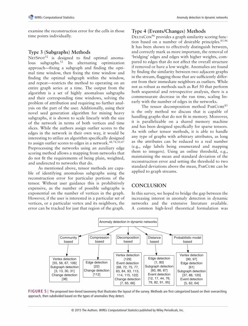
WIREs Computational Statistics Anomaly detection in dynamic networks
examine the reconstruction error for the cells in thosetime points individually.
Type 3 (Subgraphs) MethodsNetSpot52 is designed to find optimal anoma-lous subgraphs.52 Its alternating optimizationapproach—fixing a subgraph and finding the opti-mal time window, then fixing the time window andfinding the optimal subgraph within the window,and repeat—restricts the method to operating on anentire graph series at a time. The output from thealgorithm is a set of highly anomalous subgraphsand their corresponding time windows, solving theproblem of attribution and requiring no further anal-ysis on the part of the user. Additionally, using theirnovel seed generation algorithm for mining heavysubgraphs, it is shown to scale linearly with the sizeof the network in terms of both vertices and timeslices. While the authors assign outlier scores to theedges in the network in their own way, it would beinteresting to utilize an algorithm specifically designedto assign outlier scores to edges in a network.48,74,50,47
Preprocessing the networks using an auxiliary edgescoring method allows a mapping from networks thatdo not fit the requirements of being plain, weighted,and undirected to networks that do.
As mentioned above, tensor methods are capa-ble of identifying anomalous subgraphs using thereconstruction error for particular portions of thetensor. Without user guidance this is prohibitivelyexpensive, as the number of possible subgraphs isexponential on the number of vertices in the graph.However, if the user is interested in a particular set ofvertices, or a particular vertex and its neighbors, theerror can be tracked for just that region of the graph.
Type 4 (Events/Changes) MethodsDeltaCon96 provides a graph similarity scoring func-tion based on a number of desirable principles.85,96
It has been shown to effectively distinguish between,and correctly mark as more important, the removal of‘bridging’ edges and edges with higher weights, com-pared to edges that do not affect the overall structureif removed or have a low weight. Anomalies are foundby finding the similarity between two adjacent graphsin the stream, flagging those that are sufficiently differ-ent from their immediate neighbors as outliers. Whilenot as robust as methods such as Ref 50 that performboth sequential and retrospective analysis, there is acommensurate decrease in the run time, scaling lin-early with the number of edges in the networks.
The tensor decomposition method ParCube85
is the only method we discuss that is capable ofhandling graphs that do not fit in memory. Moreover,it is parallelizable on a shared memory machineand has been designed specifically for sparse tensors.As with other tensor methods, it is able to handleany type of graphs with arbitrary attributes, as longas the attributes can be reduced to a real number(e.g., edge labels being enumerated and mappingthem to integers). Using an online threshold, e.g.,maintaining the mean and standard deviation of thereconstruction error and setting the threshold to twostandard deviations above the mean, ParCube can beapplied to graph streams.
CONCLUSION
In this survey, we hoped to bridge the gap between theincreasing interest in anomaly detection in dynamicnetworks and the extensive literature available.A common high-level theoretical formulation was
Anomaly detection in dynamic networks
Community
based
Compressionbased
Decompositionbased
Distance
based
Probabilistic model
based
Vertex detection[55, 56, 67, 106]
Subgraph detection
[3, 13, 30, 31]
Change detection[38]
Edge detection
[22]Change detection
[112]
Vertex detection
[129]
Event detection[68, 72, 75, 77,83, 84, 93, 113,
114, 115, 122]Change detection
[7, 65, 66]
Edge detection[1, 80]
Subgraph detection[60, 86, 87]
Event detection[12, 17, 44, 76,79, 82, 91, 95]
Vertex detection
[90, 97]
Edge detection[61]
Subgraph detection
[37, 88, 120]Event detection
[5, 62, 64]
FIGURE 5 | The proposed two-tiered taxonomy that illustrates the layout of the survey. Methods are first categorized based on their overarchingapproach, then subdivided based on the types of anomalies they detect.
© 2015 The Authors. WIREs Computational Statistics published by Wiley Periodicals, Inc.
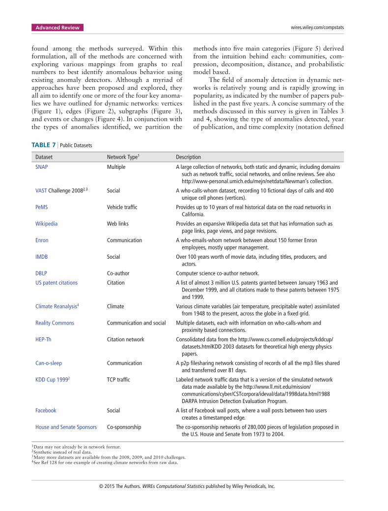
Advanced Review wires.wiley.com/compstats
found among the methods surveyed. Within thisformulation, all of the methods are concerned withexploring various mappings from graphs to realnumbers to best identify anomalous behavior usingexisting anomaly detectors. Although a myriad ofapproaches have been proposed and explored, theyall aim to identify one or more of the four key anoma-lies we have outlined for dynamic networks: vertices(Figure 1), edges (Figure 2), subgraphs (Figure 3),and events or changes (Figure 4). In conjunction withthe types of anomalies identified, we partition the
methods into five main categories (Figure 5) derivedfrom the intuition behind each: communities, com-pression, decomposition, distance, and probabilisticmodel based.
The field of anomaly detection in dynamic net-works is relatively young and is rapidly growing inpopularity, as indicated by the number of papers pub-lished in the past five years. A concise summary of themethods discussed in this survey is given in Tables 3and 4, showing the type of anomalies detected, yearof publication, and time complexity (notation defined
TABLE 7 Public Datasets
Dataset Network Type1 Description
SNAP Multiple A large collection of networks, both static and dynamic, including domainssuch as network traffic, social networks, and online reviews. See alsohttp://www-personal.umich.edu/mejn/netdata/Newman’s collection.
VAST Challenge 20082,3 Social A who-calls-whom dataset, recording 10 fictional days of calls and 400unique cell phones (vertices).
PeMS Vehicle traffic Provides up to 10 years of real historical data on the road networks inCalifornia.
Wikipedia Web links Provides an expansive Wikipedia data set that has information such aspage links, page views, and page revisions.
Enron Communication A who-emails-whom network between about 150 former Enronemployees, mostly upper management.
IMDB Social Over 100 years worth of movie data, including titles, producers, andactors.
DBLP Co-author Computer science co-author network.
US patent citations Citation A list of almost 3 million U.S. patents granted between January 1963 andDecember 1999, and all citations made to these patents between 1975and 1999.
Climate Reanalysis4 Climate Various climate variables (air temperature, precipitable water) assimilatedfrom 1948 to the present, across the globe in a fixed grid.
Reality Commons Communication and social Multiple datasets, each with information on who-calls-whom andproximity based connections.
HEP-Th Citation network Consolidated data from the http://www.cs.cornell.edu/projects/kddcup/datasets.htmlKDD 2003 datasets for theoretical high energy physicspapers.
Can-o-sleep Communication A p2p filesharing network consisting of records of all the mp3 files sharedand transferred over 81 days.
KDD Cup 19992 TCP traffic Labeled network traffic data that is a version of the simulated networkdata made available by the http://www.ll.mit.edu/mission/communications/cyber/CSTcorpora/ideval/data/1998data.html1988DARPA Intrusion Detection Evaluation Program.
Facebook Social A list of Facebook wall posts, where a wall posts between two userscreates a timestamped edge.
House and Senate Sponsors Co-sponsorship The co-sponsorship networks of 280,000 pieces of legislation proposed inthe U.S. House and Senate from 1973 to 2004.
1Data may not already be in network format.2Synthetic instead of real data.3Many more datasets are available from the 2008, 2009, and 2010 challenges.4See Ref 128 for one example of creating climate networks from raw data.
© 2015 The Authors. WIREs Computational Statistics published by Wiley Periodicals, Inc.
WIREs Computational Statistics Anomaly detection in dynamic networks
in Tables 2 and 5). A list of papers that have madetheir code available to the public is given in Table 6.Moreover, there are many publicly accessible datasetsfor testing the available methods or for personal use,see Table 7. For further reading on anomaly detectionin graphs and other domains we direct the reader toRefs 16–18, 20–22, 28, 129, 130.
NOTESa Throughout this paper we will use the terms networkand graph interchangeably.b Information on the R programming language can befound at http://www.r-project.org/
ACKNOWLEDGMENTS
The authors would like to thank the reviewers for their excellent feedback and suggestions. We would also liketo thank the authors of the work we cited who provided feedback and additional information regarding theirpapers. This work was supported in part by the DOE SDAVI Institute and the U.S. National Science Foundation(Expeditions in Computing program). In addition, this material is based upon work supported in part withfunding from the Laboratory for Analytic Sciences. Any opinions, findings, conclusions, or recommendationsexpressed in this material are those of the author(s) and do not necessarily reflect the views of the Laboratoryfor Analytic Sciences and/or any agent or entity of the United States government.
REFERENCES1. Cheng H, Tan P-N, Potter C, Klooster S. A robust
graph-based algorithm for detection and characteriza-tion of anomalies in noisy multivariate time series. In:IEEE International Conference on Data Mining Work-shops, Pisa, Italy, 2008, 349–358.
2. Cheng H, Tan P-N, Potter C , Klooster SA. Detectionand characterization of anomalies in multivariate timeseries. In: Proceedings of the 9th SIAM InternationalConference on Data Mining (SDM), Sparks, NV, 2009,413–424.
3. Chen Z, Hendrix W, Guan H, Tetteh IK, ChoudharyA, Semazzi F, Samatova NF. Discovery of extremeevents-related communities in contrasting groups ofphysical system networks. Data Min Knowl Discov2013, 27:225–258.
4. Zhang T, Zhuang X, Pande S, Lee W. Anomalouspath detection with hardware support. In: Proceedingsof the 2005 International Conference on Compilers,Architectures and Synthesis for Embedded Systems.New York: ACM; 2005, 43–54.
5. Ding Q Katenka N, Barford P, Kolaczyk E , CrovellaM. Intrusion as (anti) social communication: charac-terization and detection. In: Proceedings of the 18thACM International Conference on Knowledge Discov-ery and Data Mining (SIGKDD), Beijing, China, 2012,886–894.
6. Ghoting A, Eric Otey M, Parthasarathy S. Loaded:link-based outlier and anomaly detection in evolvingdata sets. In: Proceedings of the 4th IEEE Interna-tional Conference on Data Mining (ICDM), Brighton,UK, 2004, 387–390.
7. Jing X, Shelton CR. Intrusion detection using contin-uous time Bayesian networks. J Artif Intell Res 2010,39:745–774.
8. Priebe CE, Conroy JM, Marchette DJ, Park Y. Scanstatistics on Enron graphs. Comput Math OrganTheory 2005, 11:229–247.
9. Wang H, Tang M, Park Y, Priebe CE. Locality statis-tics for anomaly detection in time series of graphs.arXiv:1306.0267, 2013.
10. Chen F, Neill DB. Non-parametric scan statisticsfor event detection and forecasting in heterogeneoussocial media graphs. In: Proceedings of the 20th ACMSIGKDD International Conference on KnowledgeDiscovery and Data Mining. New York: ACM; 2014,1166–1175.
11. Akoglu L, McGlohon M, Faloutsos C. Odd-ball: spotting anomalies in weighted graphs. In:Advances in Knowledge Discovery and Data Mining.Berlin/Heidelberg: Springer; 2010, 410–421.
12. Eberle W, Holder L. Detecting anomalies in cargousing graph properties. In: Intelligence and Secu-rity Informatics. Berlin/Heidelberg: Springer; 2006,728–730.
13. Eberle W, Holder L. Anomaly detection in data repre-sented as graphs. Intell Data Anal 2007, 11:663–689.
14. Noble CC, Cook DJ. Graph-based anomaly detection.In: Proceedings of the 9th ACM International Con-ference on Knowledge Discovery and Data Mining(SIGKDD), Washington, DC, 2003, 631–636.
15. Barnett V, Lewis T. Outliers in Statistical Data, vol. 3.New York: John Wiley & Sons; 1994608 p.
16. Chandola V, Banerjee A, Kumar V. Anomaly detec-tion: a survey. ACM Comput Surv 2009, 41:15.
17. Chandola V, Banerjee A, Kumar V. Anomaly detectionfor discrete sequences: a survey. IEEE Trans KnowlData Eng 2012, 24:823–839.
© 2015 The Authors. WIREs Computational Statistics published by Wiley Periodicals, Inc.
Advanced Review wires.wiley.com/compstats
18. Chandola V, Mithal V, Kumar V. Comparative eval-uation of anomaly detection techniques for sequencedata. In: Proceedings of the 8th IEEE InternationalConference on Data Mining (ICDM), Pisa, Italy, 2008,743–748.
19. Hawkins DM. Identification of Outliers, vol. 11.London: Chapman and Hall; 1980.
20. Akoglu L, Tong H, Koutra D. Graph-based anomalydetection and description: a survey. Data Min KnowlDiscov 2014, 28:1–63.
21. Bilgin CC, Yener B. Dynamic network evolution:models, clustering, anomaly detection. IEEE Netw2006.
22. Gupta M, Gao J, Aggarwal CC, Han J. OutlierDetection for Temporal Data. San Rafael, CA: Morgan& Claypool Publishers; 2014.
23. Hodge VJ, Austin J. A survey of outlier detectionmethodologies. Artif Intell Rev 2004, 22:85–126.
24. Agyemang M, Barker K, Alhajj R. A comprehensivesurvey of numeric and symbolic outlier mining tech-niques. Intell Data Anal 2006, 10:521–538.
25. Brent West D. Introduction to Graph Theory, vol. 2.Upper Saddle River, NJ: Prentice Hall; 2001.
26. Balakrishnan R, Ranganathan K. A Textbook ofGraph Theory. Berlin/Heidelberg: Springer; 2012.
27. Cook DJ, Holder LB. Mining Graph Data. New York:John Wiley & Sons; 2006.
28. Samatova NF, Hendrix W, Jenkins J, Padmanabhan K,Chakraborty A. Practical Graph Mining with R. BocaRaton, FL: CRC Press; 2013.
29. Fortunato S. Community detection in graphs. PhysRep 2010, 486:75–174.
30. Lancichinetti A, Fortunato S. Community detectionalgorithms: a comparative analysis. Phys Rev E 2009,80:056117.
31. Reichardt J, Bornholdt S. Statistical mechanics ofcommunity detection. Phys Rev E 2006, 74:016110.
32. Harenberg S, Bello G, Gjeltema L, Ranshous S, Har-lalka J, Seay R, Padmanabhan K, Samatova N. Com-munity detection in large-scale networks: a surveyand empirical evaluation. WIREs Comput Stat 2014,6:426–439.
33. Rissanen J. Modeling by shortest data description.Automatica 1978, 14:465–471.
34. Rissanen J. A universal prior for integers and estima-tion by minimum description length. Ann Stat 1983,11:416–431.
35. Rissanen J. Minimum-Description-Length Principle.New York: John Wiley & Sons; 1985.
36. Grünwald P. The Minimum Description Length Prin-ciple. Cambridge, MA: MIT Press; 2007.
37. Golub GH, Reinsch C. Singular value decompositionand least squares solutions. Numerische Mathematik1970, 14:403–420.
38. Klema V, Laub AJ. The singular value decomposition:its computation and some applications. IEEE TransAutomatic Control 1980, 25:164–176.
39. Kolda TG, Bader BW. Tensor decompositions andapplications. SIAM Rev 2009, 51:455–500.
40. Gao X, Xiao B, Tao D, Li X. A survey of graph editdistance. Pattern Anal Appl 2010, 13:113–129.
41. Rahm E, Bernstein PA. A survey of approaches to auto-matic schema matching. VLDB J 2001, 10:334–350.
42. Koller D, Friedman N. Probabilistic Graphical Mod-els: Principles and Techniques. Cambridge, MA: MITPress; 2009.
43. Glaz J. Scan Statistics. Berlin/Heidelberg: Springer;2001.
44. Akoglu L, Faloutsos C. Event detection in time seriesof mobile communication graphs. 27th Army Sci Conf2010, 2:18.
45. Gao J, Liang F, Fan W, Wang C, Sun Y, Han J.On community outliers and their efficient detectionin information networks. In: Proceedings of the 16thACM International Conference on Knowledge Discov-ery and Data Mining (SIGKDD), Seattle, WA, 2010,813–822.
46. Ji T, Yang D, Gao J. Incremental local evolution-ary outlier detection for dynamic social networks.In: Machine Learning and Knowledge Discovery inDatabases. Berlin/Heidelberg: Springer; 2013, 1–15.
47. Li X, Li Z, Han J, Lee J-G. Temporal outlier detectionin vehicle traffic data. In: Proceedings of the 25th Inter-national Conference on Data Engineering (ICDE),Shanghai, China, 2009, 1319–1322.
48. James A, Tina E-R, Nishchal D. Detecting novel dis-crepancies in communication networks. In: Proceed-ings of the 10th IEEE International Conference onData Mining (ICDM), Sydney, Australia, 2010, 8–17.
49. Rattigan MJ, Jensen D. The case for anomalouslink discovery. ACM SIGKDD Explor Newsl 2005,7:41–47.
50. Heard NA, Weston DJ, Platanioti K, Hand DJ.Bayesian anomaly detection methods for social net-works. Ann Appl Stat 2010, 4:645–662.
51. Greene D, Doyle D, Cunningham P. Tracking theevolution of communities in dynamic social networks.In: 2010 International Conference on Advances inSocial Networks Analysis and Mining (ASONAM),2010, 176–183.
52. Mongiov M, Bogdanov P, Ranca R, Papalexakis EE,Faloutsos C, Singh AK. Netspot: spotting signifi-cant anomalous regions on dynamic networks. In:Proceedings of the 13th SIAM International Confer-ence on Data Mining (SDM), Austin, TX, 2013.
53. Miller BA, Beard MS, Bliss NT. Eigenspace analysisfor threat detection in social networks. In: 2011Proceedings of the 14th International Conference onInformation Fusion (FUSION), Chicago, IL, 2011,1–7.
© 2015 The Authors. WIREs Computational Statistics published by Wiley Periodicals, Inc.
WIREs Computational Statistics Anomaly detection in dynamic networks
54. Ramanathan A, Agarwal PK, Kurnikova M, Lang-mead CJ. An online approach for mining collec-tive behaviors from molecular dynamics simulations.J Comput Biol 2010, 17:309–324.
55. Saligrama V, Chen Z. Video anomaly detection basedon local statistical aggregates. In: 2012 IEEE Con-ference on Computer Vision and Pattern Recognition(CVPR), Providence, RI, 2012, 2112–2119.
56. Tran L, Navasca C, Luo J. Video detection anomaly vialow-rank and sparse decompositions. In: Image Pro-cessing Workshop (WNYIPW), 2012 Western NewYork, New York, NY, 2012, 17–20.
57. Koutra D, Papalexakis EE, Faloutsos C. Tensorsplat:spotting latent anomalies in time. In: 2012 16thPanhellenic Conference on Informatics (PCI), Piraeus,Greece, 2012, 144–149.
58. Ishibashi K, Kondoh T, Harada S, Mori T, KawaharaR, Asano S. Detecting anomalous traffic using commu-nication graphs. In: Telecommunications: The Infras-tructure for the 21st Century (WTC), Vienna, Austria,2010, 1–6
59. Suykens JAK, Vandewalle J. Least squares supportvector machine classifiers. Neural Process Lett 1999,9:293–300.
60. Breunig MM, Kriegel H-P, Ng RT, Sander J. LOF:identifying density-based local outliers. In: ACM Sig-mod Record, vol. 29. New York: ACM; 2000, 93–104.
61. Aggarwal CC, Yu PS. Outlier detection for highdimensional data. In: ACM Sigmod Record, vol. 30.New York: ACM; 2001, 37–46.
62. Angiulli F, Pizzuti C. Fast outlier detection in highdimensional spaces. In: Principles of Data Mining andKnowledge Discovery. Berlin/Heidelberg: Springer;2002, 15–27.
63. Angiulli F, Pizzuti C. Outlier mining in largehigh-dimensional data sets. IEEE Trans KnowlData Eng 2005, 17:203–215.
64. Parsons L, Haque E, Liu H. Subspace clustering forhigh dimensional data: a review. ACM SIGKDDExplor Newsl 2004, 6:90–105.
65. Srivastava AN. Enabling the discovery of recur-ring anomalies in aerospace problem reports usinghigh-dimensional clustering techniques. In: AerospaceConference, Big Sky, MT, 2006, 17 pp.
66. Pokrajac D, Lazarevic A, Latecki LJ. Incrementallocal outlier detection for data streams. In: IEEESymposium on Computational Intelligence and DataMining, Orlando, FL, 2007, 504–515.
67. Duan D, Li Y, Jin Y, Zhengding L. Community miningon dynamic weighted directed graphs. In: Proceedingsof the 1st ACM International Workshop on ComplexNetworks Meet Information & Knowledge Manage-ment. New York: ACM; 2009, 11–18.
68. Aggarwal CC, Subbian K. Event detection insocial streams. In: Proceedings of the 12th SIAM
International Conference on Data Mining (SDM),Anaheim, CA, 2012, 624–635.
69. Chen Z, Hendrix W, Samatova NF. Community-basedanomaly detection in evolutionary networks. J IntellInf Syst 2012, 39:59–85.
70. Gupta M, Gao J, Sun Y, Han J. Integrating communitymatching and outlier detection for mining evolution-ary community outliers. In: Proceedings of the 18thACM International Conference on Knowledge Discov-ery and Data Mining (SIGKDD), Beijing, China, 2012,859–867.
71. Gupta M, Gao J, Sun Y, Han J. Community trendoutlier detection using soft temporal pattern min-ing. In: Machine Learning and Knowledge Discov-ery in Databases. Berlin/Heidelberg: Springer; 2012,692–708.
72. Rossi RA, Gallagher B, Neville J, Henderson K. Mod-eling dynamic behavior in large evolving graphs. In:Proceeding of the 6th ACM International Conferenceon Web Search and Data Mining (WSDM), Rome,Italy, 2013, 667–676.
73. Araujo M, Papadimitriou S, Günnemann S, FaloutsosC, Basu P, Swami A, Papalexakis EE, Koutra D.Com2: fast automatic discovery of temporal (’comet’)communities. In: Proceedings of the 18th Pacific-AsiaConference on Knowledge Discovery and Data Mining(PAKDD), Tainan, Taiwan, 2014, 271–283.
74. Chakrabarti D. Autopart: parameter-free graph parti-tioning and outlier detection. In: Proceedings of the8th European Conference on Principles and Practiceof Knowledge Discovery in Databases (PKDD), Pisa,Italy, 2004, 112–124.
75. Sun J, Faloutsos C, Papadimitriou S, Yu PS. Graph-scope: parameter-free mining of large time-evolvinggraphs. In: Proceedings of the 13th ACM InternationalConference on Knowledge Discovery and Data Mining(SIGKDD), San Jose, CA, 2007, 687–696.
76. Ide T, Kashima H. Eigenspace-based anomaly detec-tion in computer systems. In: Proceedings of the 10thACM International Conference on Knowledge Discov-ery and Data Mining (SIGKDD), Seattle, WA, 2004,440–449.
77. Lakhina A, Crovella M, Diot C. Diagnosingnetwork-wide traffic anomalies. In: ACM SIGCOMMComputer Communication Review, vol. 34. NewYork: ACM; 2004, 219–230.
78. Sun J, Papadimitriou S, Yu PS. Window-based ten-sor analysis on high-dimensional and multi-aspectstreams. In: Proceedings of the 6th IEEE InternationalConference on Data Mining (ICDM), Hong Kong,China, 2006, 1076–1080.
79. Sun J, Tao D, Christos F. Beyond streams and graphs:dynamic tensor analysis. In: Proceedings of the 12thACM International Conference on Knowledge Discov-ery and Data Mining (SIGKDD), Philadelphia, PA,2006, 374–383.
© 2015 The Authors. WIREs Computational Statistics published by Wiley Periodicals, Inc.
Advanced Review wires.wiley.com/compstats
80. Sun J, Xie Y, Zhang H, Faloutsos C. Less is more: com-pact matrix decomposition for large sparse graphs.In: Proceedings of the 7th SIAM International Con-ference on Data Mining (SDM), Minneapolis, MN,2007.
81. Kolda TG, Sun J. Scalable tensor decompositionsfor multi-aspect data mining. In: Proceedings of the8th IEEE International Conference on Data Mining(ICDM), Pisa, Italy, 2008, 363–372.
82. Tong H, Papadimitriou S, Sun J, Yu PS, FaloutsosC. Colibri: fast mining of large static and dynamicgraphs. In: Proceedings of the 14th ACM InternationalConference on Knowledge Discovery and Data Mining(SIGKDD), Las Vegas, NV, 2008, 686–694.
83. Jiang R, Fei H, Huan J. Anomaly localization fornetwork data streams with graph joint sparse PCA.In: Proceedings of the 17th ACM International Con-ference on Knowledge Discovery and Data Mining(SIGKDD), San Diego, CA, 2011, 886–894.
84. Miller BA, Arcolano N, Beard MS, Kepner J, SchmidtMC, Bliss NT, Wolfe PJ. A scalable signal processingarchitecture for massive graph analysis. In: 2012 IEEEInternational Conference on Acoustics, Speech andSignal Processing (ICASSP), 2012, 5329–5332.
85. Papalexakis EE, Faloutsos C, Sidiropoulos ND. Par-cube: sparse parallelizable tensor decompositions.In: Machine Learning and Knowledge Discoveryin Databases. Berlin/Heidelberg: Springer; 2012,521–536.
86. Miller BA, Arcolano N, Bliss NT. Efficient anomalydetection in dynamic, attributed graphs: emergingphenomena and big data. In: 2013 IEEE InternationalConference on Intelligence and Security Informatics(ISI), Washington, DC, 2013, 179–184.
87. Yu W, Aggarwal CC, Ma S, Wang H. On anomaloushotspot discovery in graph streams. In: Proceedingsof the 13th IEEE International Conference on DataMining (ICDM), Dallas, TX, 2013.
88. Pincombe B. Anomaly detection in time series ofgraphs using Arma processes. ASOR Bull 2005, 24:2.
89. Gaston ME, Kraetzl M, Wallis WD. Using graphdiameter for change detection in dynamic networks.Australasian J Combinatorics 2006, 35:299.
90. Papadimitriou P, Dasdan A, Garcia-Molina H. Webgraph similarity for anomaly detection. J Internet ServAppl 2010, 1:19–30.
91. Arackaparambil C, Yan G. Wiki-watchdog: anomalydetection in Wikipedia through a distributional lens.In: Proceedings of the 2011 IEEE/WIC/ACM Interna-tional Conferences on Web Intelligence and IntelligentAgent Technology. Washington, DC: IEEE ComputerSociety; 2011, 257–264.
92. Quoc Le D, Jeong T, Eduardo Roman H, Won-KiHong J. Traffic dispersion graph based anomaly detec-tion. In: Proceedings of the Second Symposium on
Information and Communication Technology. NewYork: ACM; 2011, 36–41.
93. Berlingerio M, Koutra D, Eliassi-Rad T, FaloutsosC. Netsimile: a scalable approach to size-independentnetwork similarity. arXiv:1209.2684, 2012.
94. He W, Guangmin H, Zhou Y. Large-scale ip networkbehavior anomaly detection and identification usingsubstructure-based approach and multivariate timeseries mining. Telecomm Syst 2012, 50:1–13.
95. Malliaros FD, Megalooikonomou V, Faloutsos C.Fast robustness estimation in large social graphs:communities and anomaly detection. In: Proceedingsof the 12th SIAM International Conference on DataMining (SDM), Anaheim, CA, 2012, 942–953.
96. Koutra D, Vogelstein J, Faloutsos C. Deltacon: a prin-cipled massive-graph similarity function. In: Proceed-ings of the 13th SIAM International Conference onData Mining (SDM), Texas-Austin, TX, 2013.
97. Mongiovi M, Bogdanov P, Singh AK. Mining evolvingnetwork processes. In: Proceedings of the 13th IEEEInternational Conference on Data Mining (ICDM),Dallas, TX, 2013.
98. Huang Z, Dajun Zeng D. A link prediction approachto anomalous email detection. In: IEEE InternationalConference on Systems, Man and Cybernetics, SanDiego, CA, 2006, 1131–1136.
99. Pandit S, Horng Chau D, Wang S, Faloutsos C. Net-probe: a fast and scalable system for fraud detection inonline auction networks. In: Proceedings of the 16thInternational Conference on World Wide Web, Banff,Canada, 2007, 201–210.
100. Hirose S, Yamanishi K, Nakata T, Fujimaki R. Net-work anomaly detection based on Eigen equation com-pression. In: Proceedings of the 15th ACM Interna-tional Conference on Knowledge Discovery and DataMining (SIGKDD), Paris, France, 2009, 1185–1194.
101. Thompson B, Eliassi-Rad T. Dapa-v10: discoveryand analysis of patterns and anomalies in volatiletime-evolving networks. In: Notes of the 1st Workshopon Information in Networks (WIN), New York, NY,2009.
102. Djidjev H, Sandine G, Storlie C, Vander Wiel S.Graph based statistical analysis of network traffic. In:Proceedings of the Ninth Workshop on Mining andLearning with Graphs, San Diego, CA, 2011.
103. Aggarwal CC, Zhao Y, Yu PS. Outlier detection ingraph streams. In: Proceedings of the 27th Interna-tional Conference on Data Engineering (ICDE), Han-nover, Germany, 2011, 399–409.
104. Neil J, Hash C, Brugh A, Fisk M, Storlie CB. Scanstatistics for the online detection of locally anomaloussubgraphs. Technometrics 2013, 55:403–414.
105. Tantipathananandh C, Berger-Wolf T. Constant-factor approximation algorithms for identifyingdynamic communities. In: Proceedings of the 15th
© 2015 The Authors. WIREs Computational Statistics published by Wiley Periodicals, Inc.
WIREs Computational Statistics Anomaly detection in dynamic networks
ACM International Conference on Knowledge Dis-covery and Data Mining (SIGKDD), Paris, France,2009, 827–836
106. Tantipathananandh C , Berger-Wolf T. Finding com-munities in dynamic social networks. In: Proceed-ings of the 11th IEEE International Conference onData Mining (ICDM), Vancouver, Canada, 2011,1236–1241.
107. Tantipathananandh C , Berger-Wolf T, Kempe D. Aframework for community identification in dynamicsocial networks. In: Proceedings of the 13th ACMInternational Conference on Knowledge Discoveryand Data Mining (SIGKDD), San Jose, CA, 2007,717–726.
108. Gupta M, Gao J, Han J. Community distributionoutlier detection in heterogeneous information net-works. In: Machine Learning and Knowledge Discov-ery in Databases. Berlin/Heidelberg: Springer; 2013,557–573.
109. Grünwald P. A Tutorial Introduction to the MinimumDescription Length Principle. Cambridge, MA: MITPress; 2005.
110. Harshman RA. Foundations of the Parafac Procedure:Models and Conditions for an “Explanatory” Mul-timodal Factor Analysis. Los Angeles, CA: UCLA;1970.
111. Jolliffe I. Principal Component Analysis. New York:John Wiley & Sons; 2005.
112. Barnathan M, Megalooikonomou V, Faloutsos C,Faro S, Mohamed FB. Twave: high-order analysis offunctional MRI. Neuroimage 2011, 58:537–548.
113. Tucker LR. Some mathematical notes on three-modefactor analysis. Psychometrika 1966, 31:279–311.
114. Chung F, Linyuan L, Van V. Spectra of random graphswith given expected degrees. Proc Natl Acad Sci 2003,100:6313–6318.
115. Ringberg H, Soule A, Rexford J, Diot C. Sensitivityof PCA for traffic anomaly detection. ACM SIGMET-RICS Perf Eval Rev 2007, 35:109–120.
116. Chen Y, Miao D, Zhang H. Neighborhood outlierdetection. Expert Syst Appl 2010, 37:8745–8749.
117. Papadimitriou S, Kitagawa H, Gibbons PB, Falout-sos C. Loci: fast outlier detection using the localcorrelation integral. In: Proceeding of the 19th Inter-national Conference on Data Engineering, 2003,315–326.
118. Chazelle B. The Discrepancy Method: Randomnessand Complexity. Cambridge, UK: Cambridge Univer-sity Press; 2002.
119. Tong H, Lin C-Y. Non-negative residual matrix factor-ization with application to graph anomaly detection.In: SDM. Mesa, AZ: SIAM; 2011, 143–153.
120. Bogdanov P, Mongiov M, Singh AK. Mining heavysubgraphs in time-evolving networks. In: Proceedingsof the 11th IEEE International Conference on DataMining (ICDM), Vancouver, Canada, 2011, 81–90.
121. Mahadevan P, Krioukov D, Fall K, Vahdat A. Sys-tematic topology analysis and generation using degreecorrelations. In: ACM SIGCOMM Computer Com-munication Review, vol. 36. New York: ACM; 2006,135–146.
122. Sala A, Cao L, Wilson C, Zablit R, Zheng H, ZhaoBY. Measurement-calibrated graph models for socialnetwork experiments. In: Proceedings of the 19thInternational Conference on World Wide Web. NewYork: ACM; 2010, 861–870.
123. Wang J, Provan GM. Generating application-specificbenchmark models for complex systems. In: AAAI,2008, 566–571.
124. Koutra D, Ke T-Y, Kang U, Horng Polo Chau D,Kenneth Pao H-K, Faloutsos C. Unifying guilt-by-association approaches: theorems and fast algorithms.In: Machine Learning and Knowledge Discoveryin Databases. Berlin/Heidelberg: Springer; 2011,245–260.
125. Box GEP, Jenkins G. Time Series Analysis: Forecastingand Control. San Francisco, CA: Holden-Day; 1970.
126. Charikar MS. Similarity estimation techniquesfrom rounding algorithms. In: Proceedings of theThiry-Fourth Annual ACM Symposium on Theory ofComputing. New York: ACM; 2002, 380–388.
127. Gupta AK, Nagar DK. Matrix Variate Distributions,vol. 104. Boca Raton, FL: CRC Press; 1999.
128. Steinhaeuser K, Chawla NV, Ganguly AR. Complexnetworks as a unified framework for descriptive anal-ysis and predictive modeling in climate science. StatAnal Data Min 2011, 4:497–511.
129. Aggarwal CC. Outlier Analysis. Berlin/Heidelberg:Springer; 2013.
130. Gupta M, Gao J, Aggarwal CC, Han J. Outlierdetection for temporal data: a survey. IEEE TransKnowl Data Eng 2013, 25:1.
© 2015 The Authors. WIREs Computational Statistics published by Wiley Periodicals, Inc.


![Comparison of Unsupervised Anomaly Detection Techniques · a RapidMiner [10] Extension Anomaly Detection was developed that contains several unsupervised anomaly detection techniques](https://img.pdfslide.net/doc/110x75/5b014b8c7f8b9a952f8e25e8/comparison-of-unsupervised-anomaly-detection-rapidminer-10-extension-anomaly-detection.jpg)

![Anomaly Detection: Principles, Benchmarking, Explanation ...web.engr.oregonstate.edu/~tgd/...anomaly-detection... · Towards a Theory of Anomaly Detection [Siddiqui, et al.; UAI 2016]](https://img.pdfslide.net/doc/110x75/5fd8992320a65f059c333c6d/anomaly-detection-principles-benchmarking-explanation-webengr-tgdanomaly-detection.jpg)