ANTENNA LECTURES BY Abdulmuttalib A. H. …ceng.tu.edu.iq/eed/images/2019/CH1.pdfANTENNA LECTURES BY Abdulmuttalib A. H. Aldouri & Mohammed Kamil 4 1.2 Isotropic, Directional, and

ANTENNA LECTURES BY Abdulmuttalib A. H. Aldouri & Mohammed Kamil

1

ANTENNAS

Definition

An antenna is defined as a metallic device (as a rod or wire) for radiating or receiving

radio waves, so we have a transmitting antenna and a receiving antenna. In other words, the

antenna is a transitional device between free-space and a transmission line (coaxial line or a

waveguide) as shown in figure below.

Types of Antennas

1- Wire Antennas

Wire antennas are familiar to the layman because they are seen virtually everywhere on

automobiles, buildings, ships, aircraft, spacecraft, and so on. There are various shapes of wire

antennas such as a straight wire (dipole), loop, and helix which are shown below.


2

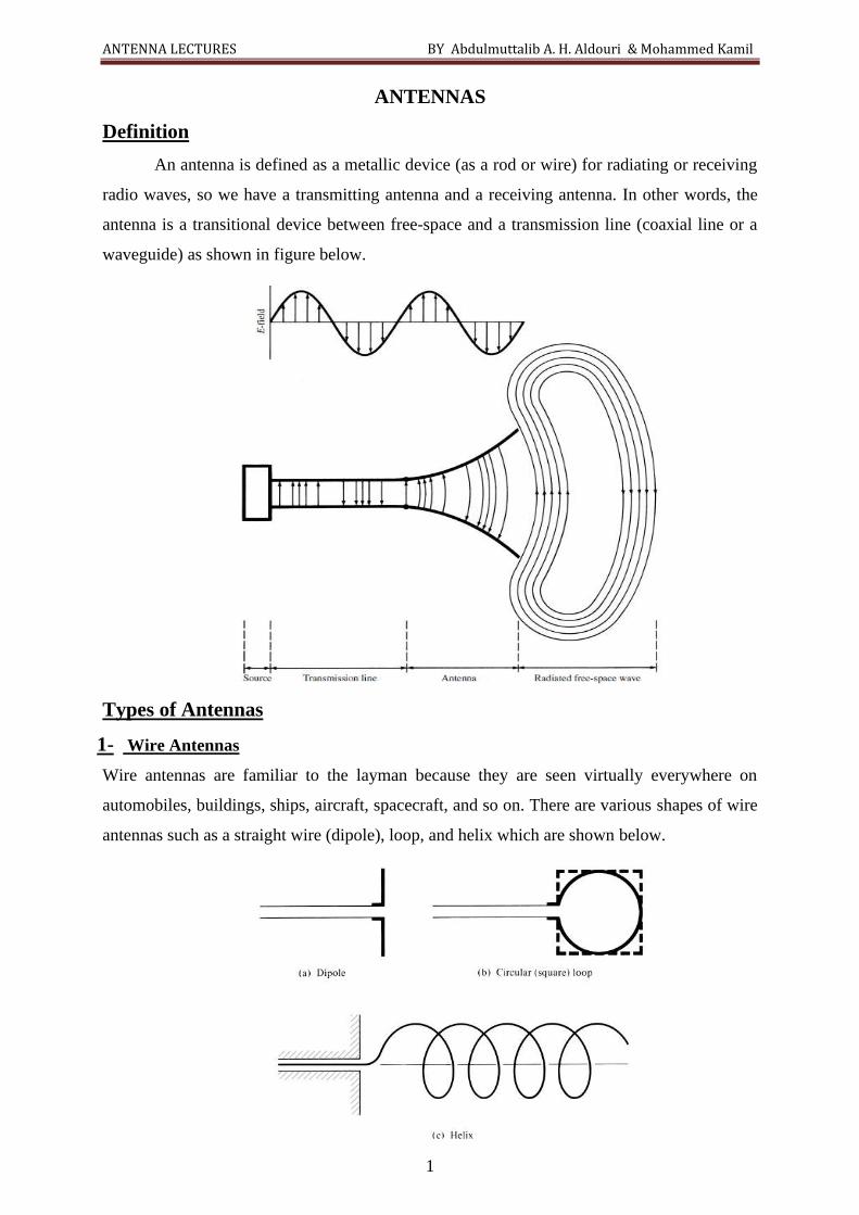
2- Aperture Antennas

Antennas of this type are very useful for aircraft and spacecraft applications, because they can

be very conveniently flush-mounted on the skin of the aircraft or spacecraft

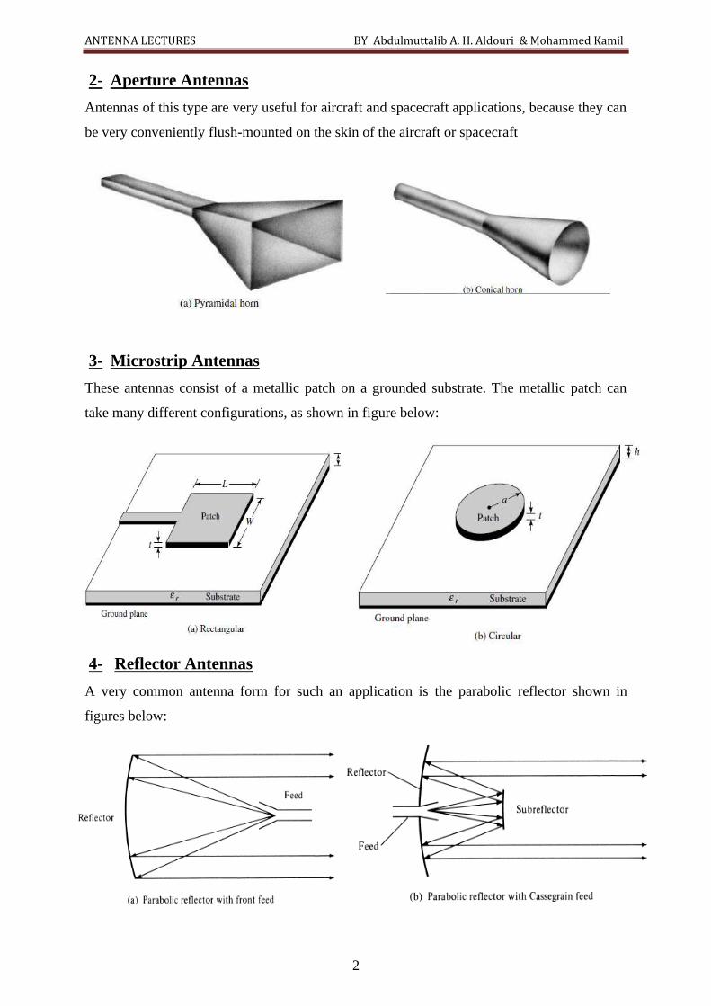
3- Microstrip Antennas

These antennas consist of a metallic patch on a grounded substrate. The metallic patch can

take many different configurations, as shown in figure below:

4- Reflector Antennas

A very common antenna form for such an application is the parabolic reflector shown in

figures below:


3

Fundamentals Parameters of Antennas

1. Radiation Pattern

An antenna radiation pattern or antenna pattern is defined as a mathematical function

or a graphical representation of the radiation properties of the antenna as a function of

space coordinates. In most cases, the radiation pattern is determined in the far field region

and is represented as a function of the directional coordinates. Radiation properties include

power flux density, radiation intensity, field strength, directivity, phase or polarization.

1.1 Radiation Pattern Lobes

Various parts of a radiation pattern are referred to as lobes, which may be

subclassified into major or main, minor, side, and back lobes as shown in figure below.

A major lobe (also called main beam) is defined as “the radiation lobe containing

the direction of maximum radiation.” In some antennas, there may exist more than

one major lobe.

A minor lobe is any lobe except a major lobe.

A side lobe is adjacent to the main lobe and occupies the hemisphere in the

direction of the mainbeam.

A back lobe is a radiation lobe whose axis makes an angle of approximately 180o

with respect to the major (main) lobe.


4

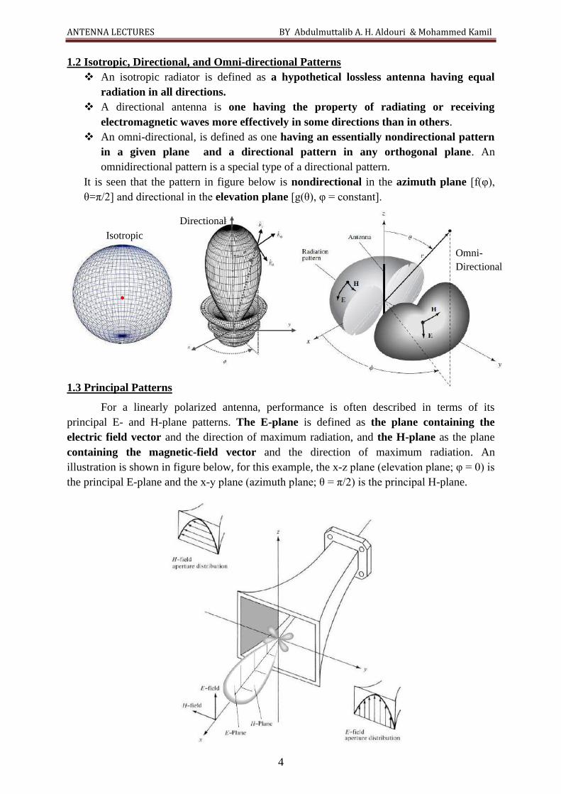
1.2 Isotropic, Directional, and Omni-directional Patterns

An isotropic radiator is defined as a hypothetical lossless antenna having equal

radiation in all directions.

A directional antenna is one having the property of radiating or receiving

electromagnetic waves more effectively in some directions than in others.

An omni-directional, is defined as one having an essentially nondirectional pattern

in a given plane and a directional pattern in any orthogonal plane. An

omnidirectional pattern is a special type of a directional pattern.

It is seen that the pattern in figure below is nondirectional in the azimuth plane [f(φ),

θ=π/2] and directional in the elevation plane [g(θ), φ = constant].

1.3 Principal Patterns

For a linearly polarized antenna, performance is often described in terms of its

principal E- and H-plane patterns. The E-plane is defined as the plane containing the

electric field vector and the direction of maximum radiation, and the H-plane as the plane

containing the magnetic-field vector and the direction of maximum radiation. An

illustration is shown in figure below, for this example, the x-z plane (elevation plane; φ = 0) is

the principal E-plane and the x-y plane (azimuth plane; θ = π/2) is the principal H-plane.

Isotropic

Directional

Omni-

Directional


5

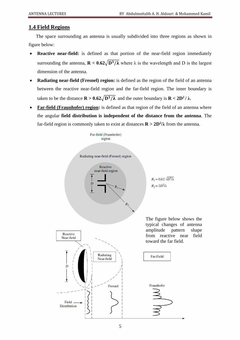
1.4 Field Regions

The space surrounding an antenna is usually subdivided into three regions as shown in

figure below:

• Reactive near-field: is defined as that portion of the near-field region immediately

surrounding the antenna, R < 0.62√𝐃𝟑/𝛌 where λ is the wavelength and D is the largest

dimension of the antenna.

• Radiating near-field (Fresnel) region: is defined as the region of the field of an antenna

between the reactive near-field region and the far-field region. The inner boundary is

taken to be the distance R > 0.62√𝐃𝟑/𝛌 and the outer boundary is R < 2D2 / λ.

• Far-field (Fraunhofer) region: is defined as that region of the field of an antenna where

the angular field distribution is independent of the distance from the antenna. The

far-field region is commonly taken to exist at distances R > 2D2/λ from the antenna.

The figure below shows the

typical changes of antenna

amplitude pattern shape

from reactive near field

toward the far field.


6

2. Radiation Power Density (W)

Power and energy are associated with electromagnetic fields. The quantity used to

describe the power associated with an electromagnetic wave is the instantaneous Poynting

vector defined as:

𝑾 = 𝑬 × 𝑯

W = instantaneous Poynting vector (W/m2)

E = instantaneous electric-field intensity (V/m)

H = instantaneous magnetic-field intensity (A/m)

The average power density can be written as:

Where η is the free space impedance 𝜂 =𝐸

𝐻= √

𝜇0

𝜀0= 120𝜋

The average power radiated by an antenna (radiated power) can be written as:

Example: The radial component of the radiated power density of an antenna is given by:

Wav = Aosinθ

r2 ar W/m2, where A0 is the peak value of the power density, determine the

total radiated power?

Solution:

𝑃𝑟𝑎𝑑 = ∫ ∫ 𝑊𝑎𝑣. 𝑑𝑠𝜋

0

2𝜋

0

𝑃𝑟𝑎𝑑 = ∫ ∫ 𝐴𝑜

𝑠𝑖𝑛𝜃

𝑟2 𝑎𝑟

𝜋

0

.2𝜋

0

𝑟2𝑠𝑖𝑛𝜃𝑑𝜃𝑑𝜙 𝑎𝑟 = 𝜋2𝐴𝑜 (𝑊)

The total power radiated of isotropic antenna is given by:

𝑃𝑟𝑎𝑑 = ∫ ∫ 𝑤𝑜 . 𝑑𝑠𝜋

0

2𝜋

0= ∫ ∫ 𝑤𝑜

𝜋

0

.2𝜋

0

𝑟2𝑠𝑖𝑛𝜃𝑑𝜃𝑑𝜙 𝑎𝑟 = 4𝜋𝑟2𝑤𝑜 (𝑊)

and the power density by:

𝑤𝑜 =𝑃𝑟𝑎𝑑

4𝜋𝑟2 𝑎𝑟

𝑊𝑎𝑣 = 𝑊𝑟𝒂𝒓 =1

2𝑅𝑒[𝐸 × 𝐻∗] =

1

2𝑅𝑒[𝐸𝜃 × 𝐻ϕ

∗ ] = −1

2𝑅𝑒[𝐸ϕ × 𝐻θ

∗] =𝐸2

2𝜂=

𝜂𝐻2

2

𝑃𝑟𝑎𝑑 = ∫ ∫ 𝑊𝑎𝑣 . 𝑑𝑠𝜋

0

2𝜋

0

= ∫ ∫ 𝑊𝑟𝒂𝒓 . 𝑟2𝑠𝑖𝑛𝜃𝑑𝜃𝑑ϕ 𝒂𝒓

𝜋

0

2𝜋

0

, 𝑑𝑠 = 𝑟2𝑠𝑖𝑛𝜃𝑑𝜃𝑑ϕ 𝑎𝑟


7

3. Radiation Intensity (U)

Radiation intensity in a given direction is defined as “the power radiated from an

antenna per unit solid angle.” In a mathematical form, it is expressed as:

𝑼 = 𝒓𝟐𝑾𝒓𝒂𝒅

"U" is the radiation intensity (W/unit solid angle)

Wrad: radiation density (W/m2)

𝑷𝒓𝒂𝒅 = ∫ ∫ 𝑼.𝒅Ω𝝅

𝟎

𝟐𝝅

𝟎

= ∫ ∫ 𝑼.𝝅

𝟎

𝟐𝝅

𝟎

𝒔𝒊𝒏𝜽𝒅𝜽𝒅𝛟

(dΩ) =Unit solid angle = sinθdθdϕ

𝑷𝒓𝒂𝒅 = 𝑰𝒓𝒎𝒔𝟐 𝑹𝒓𝒂𝒅 =

𝑰𝟎𝟐

𝟐𝑹𝒓𝒂𝒅 𝑹𝒓𝒂𝒅 = 𝒓𝒂𝒅𝒊𝒂𝒕𝒊𝒐𝒏 𝒓𝒆𝒔𝒊𝒔𝒕𝒂𝒏𝒄𝒆

The radiation intensity of an isotropic source as:

𝑼𝒐 =𝑷𝒓𝒂𝒅

𝟒𝝅

Example: The power radiated by a lossless antenna is 10 watts. The directional

characteristics of the antenna are represented by the radiation intensity of

𝐚) 𝐔 = 𝐁𝟎𝐜𝐨𝐬𝟐(𝛉) 𝐛) 𝐔 = 𝐁𝟎𝐜𝐨𝐬𝟑(𝛉) 𝟎 ≤ 𝛉 ≤𝛑

𝟐 𝟎 ≤ ∅ ≤ 𝟐𝛑

For each, find the maximum power density (in watts/square meter) at a distance of 1000m?

Solution:


8

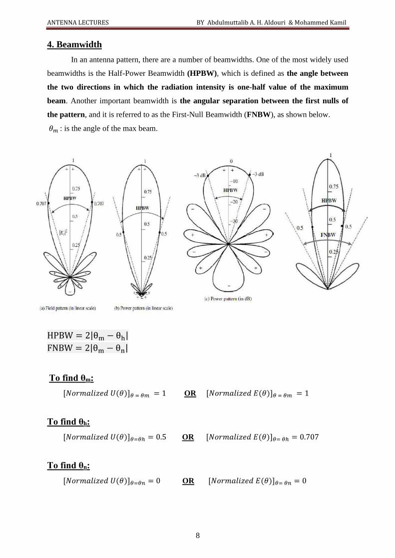
4. Beamwidth

In an antenna pattern, there are a number of beamwidths. One of the most widely used

beamwidths is the Half-Power Beamwidth (HPBW), which is defined as the angle between

the two directions in which the radiation intensity is one-half value of the maximum

beam. Another important beamwidth is the angular separation between the first nulls of

the pattern, and it is referred to as the First-Null Beamwidth (FNBW), as shown below.

𝜃𝑚 : is the angle of the max beam.

HPBW = 2|θm − θh|

FNBW = 2|θm − θn|

To find θm:

[𝑁𝑜𝑟𝑚𝑎𝑙𝑖𝑧𝑒𝑑 𝑈(𝜃)]𝜃 = 𝜃𝑚 = 1 OR [𝑁𝑜𝑟𝑚𝑎𝑙𝑖𝑧𝑒𝑑 𝐸(𝜃)]𝜃 = 𝜃𝑚 = 1

To find θh:

[𝑁𝑜𝑟𝑚𝑎𝑙𝑖𝑧𝑒𝑑 𝑈(𝜃)]𝜃=𝜃ℎ = 0.5 OR [𝑁𝑜𝑟𝑚𝑎𝑙𝑖𝑧𝑒𝑑 𝐸(𝜃)]𝜃= 𝜃ℎ = 0.707

To find θn:

[𝑁𝑜𝑟𝑚𝑎𝑙𝑖𝑧𝑒𝑑 𝑈(𝜃)]𝜃=𝜃𝑛 = 0 OR [𝑁𝑜𝑟𝑚𝑎𝑙𝑖𝑧𝑒𝑑 𝐸(𝜃)]𝜃= 𝜃𝑛 = 0


9

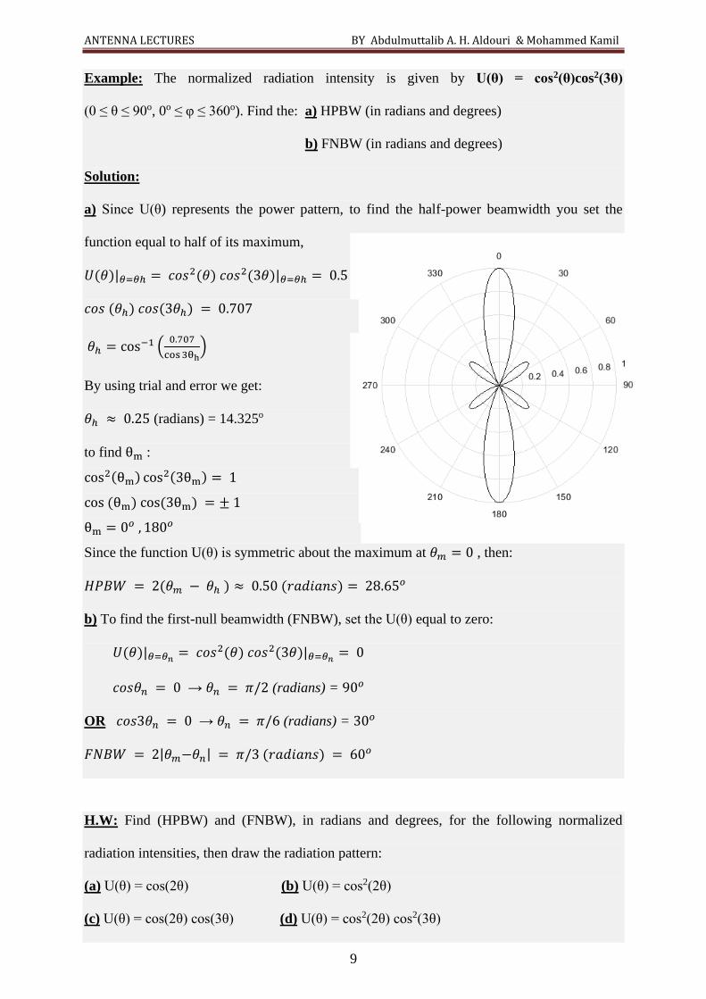
Example: The normalized radiation intensity is given by U(θ) = cos2(θ)cos2(3θ)

(0 ≤ θ ≤ 90o, 0o ≤ φ ≤ 360o). Find the: a) HPBW (in radians and degrees)

b) FNBW (in radians and degrees)

Solution:

a) Since U(θ) represents the power pattern, to find the half-power beamwidth you set the

function equal to half of its maximum,

𝑈(𝜃)|𝜃=𝜃ℎ = 𝑐𝑜𝑠2(𝜃) 𝑐𝑜𝑠2(3𝜃)|𝜃=𝜃ℎ = 0.5

𝑐𝑜𝑠 (𝜃ℎ) 𝑐𝑜𝑠(3𝜃ℎ) = 0.707

𝜃ℎ = cos−1 (0.707

cos3θh)

By using trial and error we get:

𝜃ℎ ≈ 0.25 (radians) = 14.325o

to find θm :

cos2(θm) cos2(3θm) = 1

cos (θm) cos(3θm) = ± 1

θm = 0𝑜 , 180𝑜

Since the function U(θ) is symmetric about the maximum at 𝜃𝑚 = 0 , then:

𝐻𝑃𝐵𝑊 = 2(𝜃𝑚 − 𝜃ℎ ) ≈ 0.50 (𝑟𝑎𝑑𝑖𝑎𝑛𝑠) = 28.65𝑜

b) To find the first-null beamwidth (FNBW), set the U(θ) equal to zero:

𝑈(𝜃)|𝜃=𝜃𝑛= 𝑐𝑜𝑠2(𝜃) 𝑐𝑜𝑠2(3𝜃)|𝜃=𝜃𝑛

= 0

𝑐𝑜𝑠𝜃𝑛 = 0 → 𝜃𝑛 = 𝜋/2 (radians) = 90𝑜

OR 𝑐𝑜𝑠3𝜃𝑛 = 0 → 𝜃𝑛 = 𝜋/6 (radians) = 30𝑜

𝐹𝑁𝐵𝑊 = 2|𝜃𝑚−𝜃𝑛| = 𝜋/3 (𝑟𝑎𝑑𝑖𝑎𝑛𝑠) = 60𝑜

H.W: Find (HPBW) and (FNBW), in radians and degrees, for the following normalized

radiation intensities, then draw the radiation pattern:

(a) U(θ) = cos(2θ) (b) U(θ) = cos2(2θ)

(c) U(θ) = cos(2θ) cos(3θ) (d) U(θ) = cos2(2θ) cos2(3θ)


10

5. Directivity D

Directivity of an antenna is defined as the ratio of the radiation intensity in a given

direction from the antenna to the radiation intensity averaged over all directions. In

mathematical form, it can be written as:

𝑫 =𝑼

𝑼𝒐=

𝟒𝝅𝑼

𝑷𝒓𝒂𝒅 (𝒅𝒊𝒎𝒆𝒏𝒔𝒊𝒐𝒏𝒍𝒆𝒔𝒔)

The maximum directivity is expressed as:

𝑫𝒎𝒂𝒙 = 𝑫𝒐 =𝑼𝒎𝒂𝒙

𝑼𝒐=

𝟒𝝅𝑼𝒎𝒂𝒙

𝑷𝒓𝒂𝒅 (𝒅𝒊𝒎𝒆𝒏𝒔𝒊𝒐𝒏𝒍𝒆𝒔𝒔)

The general expression for the directivity and maximum directivity is:

𝑫(𝜽,𝝓) = 𝟒𝝅𝑼(𝜽,𝝓)

∫ ∫ 𝑼(𝜽,𝝓) 𝒔𝒊𝒏𝜽𝒅𝜽𝒅𝝓𝝅

𝟎

𝟐𝝅

𝟎

𝑫𝒎𝒂𝒙 = 𝟒𝝅𝑼(𝜽,𝝓)|𝒎𝒂𝒙

∫ ∫ 𝑼(𝜽,𝝓) 𝒔𝒊𝒏𝜽𝒅𝜽𝒅𝝓𝝅

𝟎

𝟐𝝅

𝟎

=𝟒𝝅

Ω𝑨

Where ΩA is the beam solid angle, and it is given by:

Ω𝑨 = ∫ ∫ 𝑼𝒏(𝜽,𝝓) 𝒔𝒊𝒏𝜽𝒅𝜽𝒅𝝓𝝅

𝟎

𝟐𝝅

𝟎

Example: The radiation intensity of the major lobe of many antennas can be adequately

represented by: 𝐔(𝛉) = 𝐁𝟎 𝐜𝐨𝐬𝛉. The radiation intensity exists only in the upper

hemisphere (0 ≤ θ ≤ π/2, 0 ≤ φ ≤ 2π), find the maximum directivity D?

Solution:

U𝑛(θ) = cosθ

ΩA = ∫ ∫ cosθ sinθdθdϕ = 2π ∗1

2∫ sin(2θ) dθ = π

π/2

0

π/2

0

2π

0

Dmax =4π

ΩA=

4π

π= 4 = 6.02 dB


11

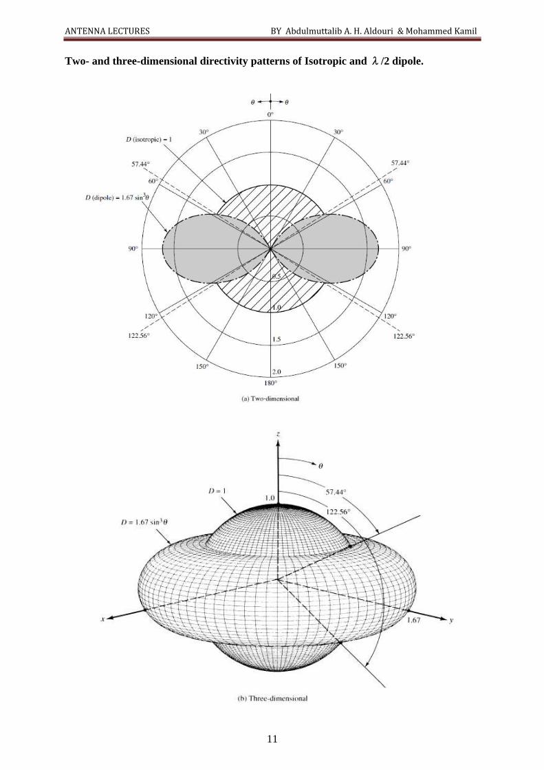
Two- and three-dimensional directivity patterns of Isotropic and λ/2 dipole.


12

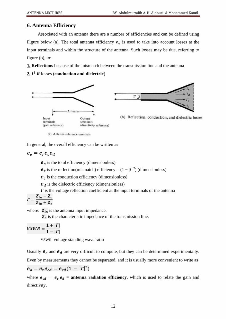
6. Antenna Efficiency

Associated with an antenna there are a number of efficiencies and can be defined using

Figure below (a). The total antenna efficiency 𝒆𝒐 is used to take into account losses at the

input terminals and within the structure of the antenna. Such losses may be due, referring to

figure (b), to:

1. Reflections because of the mismatch between the transmission line and the antenna

2. 𝑰𝟐 𝑹 losses (conduction and dielectric)

In general, the overall efficiency can be written as

𝒆𝒐 = 𝒆𝒓𝒆𝒄𝒆𝒅

𝒆𝒐 is the total efficiency (dimensionless)

𝒆𝒓 is the reflection(mismatch) efficiency = (1 − |𝛤|2) (dimensionless)

𝒆𝒄 is the conduction efficiency (dimensionless)

𝒆𝒅 is the dielectric efficiency (dimensionless)

𝜞 is the voltage reflection coefficient at the input terminals of the antenna

𝜞 =𝒁𝒊𝒏 − 𝒁𝐨

𝒁𝒊𝒏 + 𝒁𝐨

where: 𝒁𝒊𝒏 is the antenna input impedance,

𝒁𝒐 is the characteristic impedance of the transmission line.

𝑽𝑺𝑾𝑹 =𝟏 + |𝜞|

𝟏 − |𝜞|

VSWR: voltage standing wave ratio

Usually 𝒆𝒄 and 𝒆𝒅 are very difficult to compute, but they can be determined experimentally.

Even by measurements they cannot be separated, and it is usually more convenient to write as

𝒆𝒐 = 𝒆𝒓𝒆𝒄𝒅 = 𝒆𝒄𝒅(𝟏 − |𝜞|𝟐)

where 𝒆𝒄𝒅 = 𝒆𝒄 𝒆𝒅 = antenna radiation efficiency, which is used to relate the gain and

directivity.


13

7. Gain

Gain of an antenna is defined as the ratio of the radiation intensity, in a given

direction, to the radiation intensity that would be obtained if the power accepted by the

antenna were radiated isotropically.

𝑮 =𝒓𝒂𝒅𝒊𝒂𝒕𝒊𝒐𝒏 𝒊𝒏𝒕𝒆𝒏𝒔𝒊𝒕𝒚

𝒕𝒐𝒕𝒂𝒍 𝒊𝒏𝒑𝒖𝒕 (𝒂𝒄𝒄𝒆𝒑𝒕𝒆𝒅) 𝒑𝒐𝒘𝒆𝒓/𝟒𝝅= 𝟒𝝅

𝑼(𝜽,𝝓)

𝑷𝒊𝒏

According to the IEEE Standards, “gain does not include losses arising from impedance

mismatches (reflection losses) and polarization mismatches (losses).”

𝑷𝒓𝒂𝒅 = 𝒆𝒄𝒅 𝑷𝒊𝒏

which is related to the directivity by:

𝑮(𝜽,𝝓) = 𝒆𝒄𝒅 [𝟒𝝅𝑼(𝜽,𝝓)

𝑷𝒓𝒂𝒅] = 𝒆𝒄𝒅 𝑫(𝜽,𝝓) → 𝐆𝐦𝐚𝐱 = 𝒆𝒄𝒅 𝑫𝒎𝒂𝒙

We can introduce an absolute gain 𝑮𝒂𝒃𝒔 that takes into account the reflection/mismatch

losses (due to the connection of the antenna to the transmission line), and it can be written as:

𝑮𝒂𝒃𝒔 = 𝒆𝒓𝒆𝒄𝒅 𝑫 = 𝒆𝒄𝒅(𝟏 − |𝜞|𝟐) 𝑫

Example: A lossless antenna, with input impedance of 73 Ω, is connected to a transmission

line whose characteristics impedance is 50 Ω, assuming that the pattern of the antenna is

given by 𝑼 = 𝟓 𝒔𝒊𝒏𝟑 𝜽 . Find the maximum absolute gain of this antenna?

Solution:


14

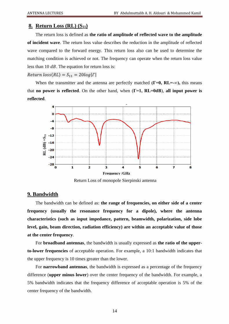
8. Return Loss (RL) (S11)

The return loss is defined as the ratio of amplitude of reflected wave to the amplitude

of incident wave. The return loss value describes the reduction in the amplitude of reflected

wave compared to the forward energy. This return loss also can be used to determine the

matching condition is achieved or not. The frequency can operate when the return loss value

less than 10 𝑑𝐵. The equation for return loss is:

𝑅𝑒𝑡𝑢𝑟𝑛 𝑙𝑜𝑠𝑠(𝑅𝐿) = 𝑆11 = 20𝑙𝑜𝑔|𝛤|

When the transmitter and the antenna are perfectly matched (Γ=0, RL=-∞), this means

that no power is reflected. On the other hand, when (Γ=1, RL=0dB), all input power is

reflected.

Return Loss of monopole Sierpinski antenna

9. Bandwidth

The bandwidth can be defined as: the range of frequencies, on either side of a center

frequency (usually the resonance frequency for a dipole), where the antenna

characteristics (such as input impedance, pattern, beamwidth, polarization, side lobe

level, gain, beam direction, radiation efficiency) are within an acceptable value of those

at the center frequency.

For broadband antennas, the bandwidth is usually expressed as the ratio of the upper-

to-lower frequencies of acceptable operation. For example, a 10:1 bandwidth indicates that

the upper frequency is 10 times greater than the lower.

For narrowband antennas, the bandwidth is expressed as a percentage of the frequency

difference (upper minus lower) over the center frequency of the bandwidth. For example, a

5% bandwidth indicates that the frequency difference of acceptable operation is 5% of the

center frequency of the bandwidth.

Frequency /GHz

RL

(d

B)

=S

11


15

10. Polarization

Polarization is defined as the orientation of electric field. In addition, polarization

describes the time varying direction and relative magnitude of the electric field vector.

Polarization may be classified as linear, circular or elliptical.

a- If the vector that describes the electric field at a point in space is always directed

along a line the field is said to be linearly polarized.

b- The figure that the electric field traces is an ellipse is said to be elliptically polarized.

Linear and circular polarizations are special cases of elliptical and they can be obtained

when the ellipse becomes a straight line or a circle respectively. The ratio of the major axis to

the minor axis is referred to as the axial ratio (AR), and it is equal to:

𝑨𝑹 =𝒎𝒂𝒋𝒐𝒓 𝒂𝒙𝒊𝒔

𝒎𝒊𝒏𝒐𝒓 𝒂𝒙𝒊𝒔=

𝑶𝑨

𝑶𝑩 𝟏 ≤ 𝑨𝑹 ≤ ∞

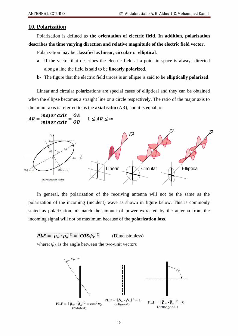
In general, the polarization of the receiving antenna will not be the same as the

polarization of the incoming (incident) wave as shown in figure below. This is commonly

stated as polarization mismatch the amount of power extracted by the antenna from the

incoming signal will not be maximum because of the polarization loss.

𝑷𝑳𝑭 = |𝝆𝒘 ∙ 𝝆𝒂 |𝟐 = |𝑪𝑶𝑺𝝍𝑷|𝟐 (Dimensionless)

where: 𝜓𝑃 is the angle between the two-unit vectors


16

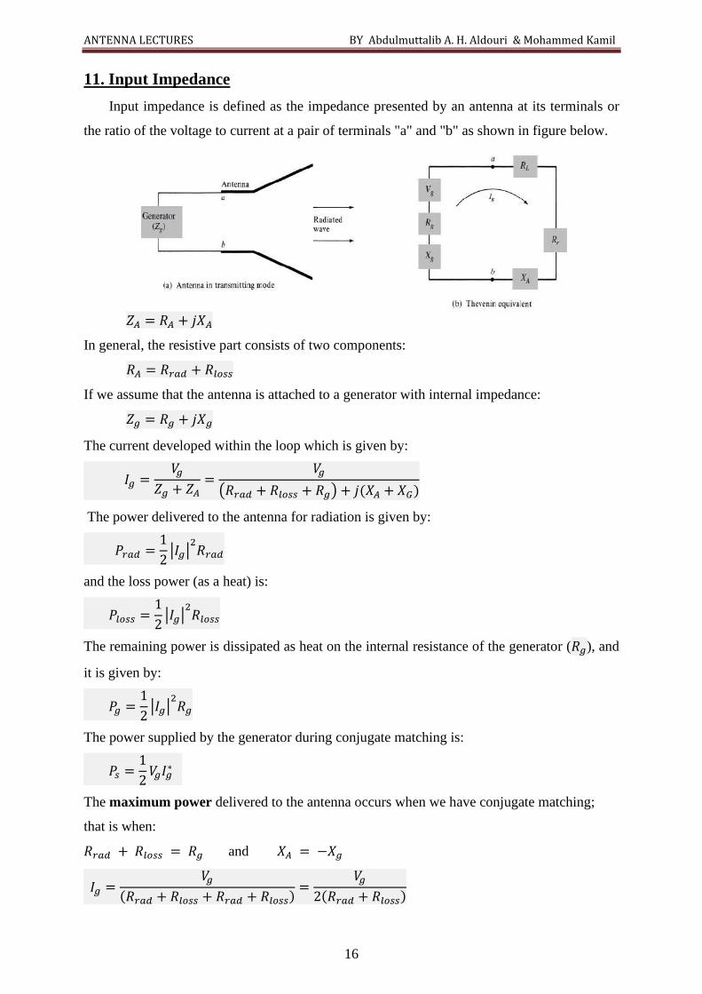
11. Input Impedance

Input impedance is defined as the impedance presented by an antenna at its terminals or

the ratio of the voltage to current at a pair of terminals "a" and "b" as shown in figure below.

𝑍𝐴 = 𝑅𝐴 + 𝑗𝑋𝐴

In general, the resistive part consists of two components:

𝑅𝐴 = 𝑅𝑟𝑎𝑑 + 𝑅𝑙𝑜𝑠𝑠

If we assume that the antenna is attached to a generator with internal impedance:

𝑍𝑔 = 𝑅𝑔 + 𝑗𝑋𝑔

The current developed within the loop which is given by:

𝐼𝑔 =𝑉𝑔

𝑍𝑔 + 𝑍𝐴=

𝑉𝑔

(𝑅𝑟𝑎𝑑 + 𝑅𝑙𝑜𝑠𝑠 + 𝑅𝑔) + 𝑗(𝑋𝐴 + 𝑋𝐺)

The power delivered to the antenna for radiation is given by:

𝑃𝑟𝑎𝑑 =1

2|𝐼𝑔|

2𝑅𝑟𝑎𝑑

and the loss power (as a heat) is:

𝑃𝑙𝑜𝑠𝑠 =1

2|𝐼𝑔|

2𝑅𝑙𝑜𝑠𝑠

The remaining power is dissipated as heat on the internal resistance of the generator (𝑅𝑔), and

it is given by:

𝑃𝑔 =1

2|𝐼𝑔|

2𝑅𝑔

The power supplied by the generator during conjugate matching is:

𝑃𝑠 =1

2𝑉𝑔𝐼𝑔

∗

The maximum power delivered to the antenna occurs when we have conjugate matching;

that is when:

𝑅𝑟𝑎𝑑 + 𝑅𝑙𝑜𝑠𝑠 = 𝑅𝑔 and 𝑋𝐴 = −𝑋𝑔

𝐼𝑔 =𝑉𝑔

(𝑅𝑟𝑎𝑑 + 𝑅𝑙𝑜𝑠𝑠 + 𝑅𝑟𝑎𝑑 + 𝑅𝑙𝑜𝑠𝑠)=

𝑉𝑔

2(𝑅𝑟𝑎𝑑 + 𝑅𝑙𝑜𝑠𝑠)


17

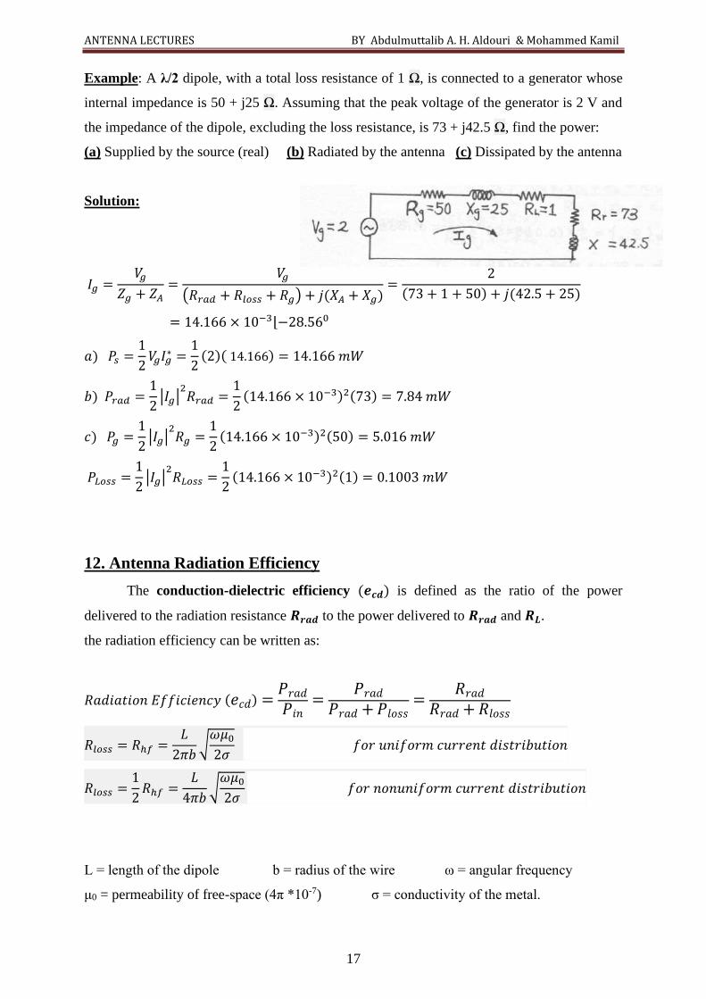
Example: A λ/2 dipole, with a total loss resistance of 1 Ω, is connected to a generator whose

internal impedance is 50 + j25 Ω. Assuming that the peak voltage of the generator is 2 V and

the impedance of the dipole, excluding the loss resistance, is 73 + j42.5 Ω, find the power:

(a) Supplied by the source (real) (b) Radiated by the antenna (c) Dissipated by the antenna

Solution:

𝐼𝑔 =𝑉𝑔

𝑍𝑔 + 𝑍𝐴=

𝑉𝑔

(𝑅𝑟𝑎𝑑 + 𝑅𝑙𝑜𝑠𝑠 + 𝑅𝑔) + 𝑗(𝑋𝐴 + 𝑋𝑔)=

2

(73 + 1 + 50) + 𝑗(42.5 + 25)

= 14.166 × 10−3⌊−28.560

𝑎) 𝑃𝑠 =1

2𝑉𝑔𝐼𝑔

∗ =1

2(2)( 14.166) = 14.166 𝑚𝑊

𝑏) 𝑃𝑟𝑎𝑑 =1

2|𝐼𝑔|

2𝑅𝑟𝑎𝑑 =

1

2(14.166 × 10−3)2(73) = 7.84 𝑚𝑊

𝑐) 𝑃𝑔 =1

2|𝐼𝑔|

2𝑅𝑔 =

1

2(14.166 × 10−3)2(50) = 5.016 𝑚𝑊

𝑃𝐿𝑜𝑠𝑠 =1

2|𝐼𝑔|

2𝑅𝐿𝑜𝑠𝑠 =

1

2(14.166 × 10−3)2(1) = 0.1003 𝑚𝑊

12. Antenna Radiation Efficiency

The conduction-dielectric efficiency (𝒆𝒄𝒅) is defined as the ratio of the power

delivered to the radiation resistance 𝑹𝒓𝒂𝒅 to the power delivered to 𝑹𝒓𝒂𝒅 and 𝑹𝑳.

the radiation efficiency can be written as:

𝑅𝑎𝑑𝑖𝑎𝑡𝑖𝑜𝑛 𝐸𝑓𝑓𝑖𝑐𝑖𝑒𝑛𝑐𝑦 (𝑒𝑐𝑑) =𝑃𝑟𝑎𝑑

𝑃𝑖𝑛=

𝑃𝑟𝑎𝑑

𝑃𝑟𝑎𝑑 + 𝑃𝑙𝑜𝑠𝑠=

𝑅𝑟𝑎𝑑

𝑅𝑟𝑎𝑑 + 𝑅𝑙𝑜𝑠𝑠

𝑅𝑙𝑜𝑠𝑠 = 𝑅ℎ𝑓 =𝐿

2𝜋𝑏√

𝜔𝜇0

2𝜎 𝑓𝑜𝑟 𝑢𝑛𝑖𝑓𝑜𝑟𝑚 𝑐𝑢𝑟𝑟𝑒𝑛𝑡 𝑑𝑖𝑠𝑡𝑟𝑖𝑏𝑢𝑡𝑖𝑜𝑛

𝑅𝑙𝑜𝑠𝑠 =1

2𝑅ℎ𝑓 =

𝐿

4𝜋𝑏√

𝜔𝜇0

2𝜎 𝑓𝑜𝑟 𝑛𝑜𝑛𝑢𝑛𝑖𝑓𝑜𝑟𝑚 𝑐𝑢𝑟𝑟𝑒𝑛𝑡 𝑑𝑖𝑠𝑡𝑟𝑖𝑏𝑢𝑡𝑖𝑜𝑛

L = length of the dipole b = radius of the wire ω = angular frequency

μ0 = permeability of free-space (4π *10-7) σ = conductivity of the metal.


18

Example: A resonant half-wavelength dipole is made out of copper (σ = 5.7 × 107 S/m) wire.

Determine the radiation efficiency of the dipole antenna at 𝑓 = 100 MHz if the radius of the

wire b=3×10−4λ, and the radiation resistance of the λ/2 dipole is 73Ω.

Solution:

λ = c/f = 3 × 108/108= 3 m

L = λ/2 = 1.5 m

For a λ/2 dipole with a sinusoidal current distribution:

𝑅𝑙𝑜𝑠𝑠 = 0.5𝑅ℎ𝑓

𝑅𝑙𝑜𝑠𝑠 = 0.51.5

2𝜋 ∗ 3 × 10−4 ∗ 3√

𝜋(108)(4𝜋 × 10−7)

5.7 × 107= 0.349Ω

𝑒𝑐𝑑 =𝑅𝑟𝑎𝑑

𝑅𝑟𝑎𝑑 + 𝑅𝑙𝑜𝑠𝑠=

73

73 + 0.349= 0.9952 = 99.52%

13. Effective Aperture (Area)

Effective aperture is defined as “the ratio of the available power at the terminals of a

receiving antenna to the power flux density of a plane wave incident on the antenna from that

direction.

The relationship between directivity and effective aperture is illustrated by the following

formulas:

𝐴𝑒 =𝜆2

4𝜋𝐷 𝑎𝑛𝑑 𝐴𝑒𝑚𝑎𝑥 =

𝜆2

4𝜋𝐷max

Example: Find the maximum directivity and the maximum effective aperture of the antenna

whose radiation intensity is 𝑈 = 𝐴𝑜𝑠𝑖𝑛𝜃 and λ = 3m. Write an expression for the directivity

as a function of the directional angles θ and φ.

Solution:

The radiation intensity is given by:

U = A0 sin θ

The maximum radiation is directed along θm = π/2, thus:

Umax = A0 and Prad = π2A0

𝐷𝑚𝑎𝑥 =4𝜋𝑈𝑚𝑎𝑥

𝑃𝑟𝑎𝑑=

4

𝜋= 1.27 , 𝐴𝑒𝑚 =

32

4𝜋∗ 1.27 = 0.9 𝑚2

D = Dmax sinθ = 1.27 sinθ


19

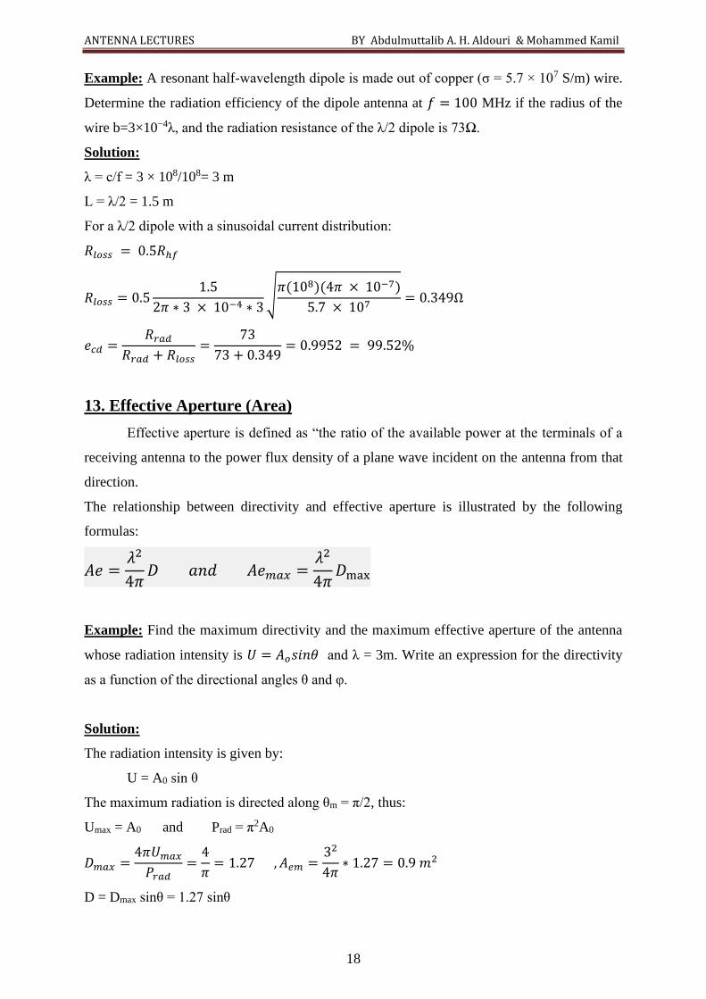
Example: The radiation intensity of an antenna is given by: 𝑼 = 𝑩𝑰𝟎𝟐 𝒔𝒊𝒏(𝝅𝒔𝒊𝒏𝜽) Find:

• Radiation power and Radiation resistance

• Maximum directivity

• Maximum effective aperture

• HPBW and FNBW

• Sketch the power pattern

Solution:

𝑃𝑟𝑎𝑑 = ∫ ∫ 𝐵𝐼02 𝑠𝑖𝑛(𝜋 𝑠𝑖𝑛 𝜃) 𝑠𝑖𝑛𝜃𝑑𝜃𝑑𝜙

𝜋

0

2𝜋

0

= 2𝜋𝐵𝐼02 ∫ 𝑠𝑖𝑛(𝜋 𝑠𝑖𝑛 𝜃) 𝑠𝑖𝑛𝜃𝑑𝜃

𝜋

0

This integral can be solved numerically (Trapezoidal or Simpson's rule)

θi 0 18 36 54 72 90 108 126 144 162 180

F(θi) 0 0.255 0.565 0.456 0.145 0 0.145 0.456 0.565 0.255 0

∫ 𝑠𝑖𝑛(𝜋 𝑠𝑖𝑛 𝜃) 𝑠𝑖𝑛𝜃𝑑𝜃𝜋

0

=𝜋/10

2[(𝑓(0) + 𝑓(𝜋)) + 2∑𝑓(𝜃𝑖)]

𝑃𝑟𝑎𝑑 = 2𝜋 ∗ 0.9𝐵𝐼02 = 1.8𝜋𝐵𝐼0

2 (𝑊)

𝑅𝑟𝑎𝑑 =2𝑃𝑟𝑎𝑑

𝐼02 = 3.6π𝐵 (Ω)

𝐷𝑚𝑎𝑥 =4𝜋𝑈𝑚𝑎𝑥

𝑃𝑟𝑎𝑑=

4𝜋𝐵𝐼02

1.8𝜋𝐵𝐼02 = 2.222

𝐴𝑒𝑚𝑎𝑥 =𝜆2

4𝜋𝐷𝑚𝑎𝑥 =

2.22

4𝜋𝜆2 = 0.177𝜆2 (𝑚2)

𝑈(𝜃)|𝜃=𝜃𝑚= 𝑠𝑖𝑛(𝜋 𝑠𝑖𝑛 𝜃𝑚) = 1 → 𝜋 𝑠𝑖𝑛 𝜃𝑚 =

𝜋

2 → 𝑠𝑖𝑛 𝜃𝑚 =

1

2 → 𝜃𝑚 = 30𝑜 and 150𝑜

𝑈(𝜃)|𝜃=𝜃ℎ= 𝑠𝑖𝑛(𝜋 𝑠𝑖𝑛 𝜃ℎ) = 0.5 →

𝜋 𝑠𝑖𝑛 𝜃ℎ =𝜋

6 → 𝑠𝑖𝑛 𝜃ℎ =

1

6 → 𝜃ℎ = 9.6𝑜

𝜋 𝑠𝑖𝑛 𝜃ℎ =5𝜋

6 → 𝑠𝑖𝑛 𝜃ℎ =

5

6 → 𝜃ℎ = 56.4𝑜

𝐻𝑃𝐵𝑊 = 56.4𝑜 − 9.6𝑜 = 46.8𝑜

𝑈(𝜃)|𝜃=𝜃𝑛= 𝑠𝑖𝑛(𝜋 𝑠𝑖𝑛 𝜃𝑛) = 0

→ 𝜋 𝑠𝑖𝑛 𝜃𝑛 = 0 → 𝑠𝑖𝑛 𝜃𝑛 = 0 → 𝜃𝑛 = 0𝑜 and 180𝑜

𝜋 𝑠𝑖𝑛 𝜃𝑛 = 𝜋 → 𝑠𝑖𝑛 𝜃𝑛 = 1 → 𝜃𝑛 = 90𝑜

𝐹𝑁𝐵𝑊 = 90𝑜 − 0𝑜 = 90𝑜

H.W: Repeat with U = BI02 cos (

π

2cos θ)


20

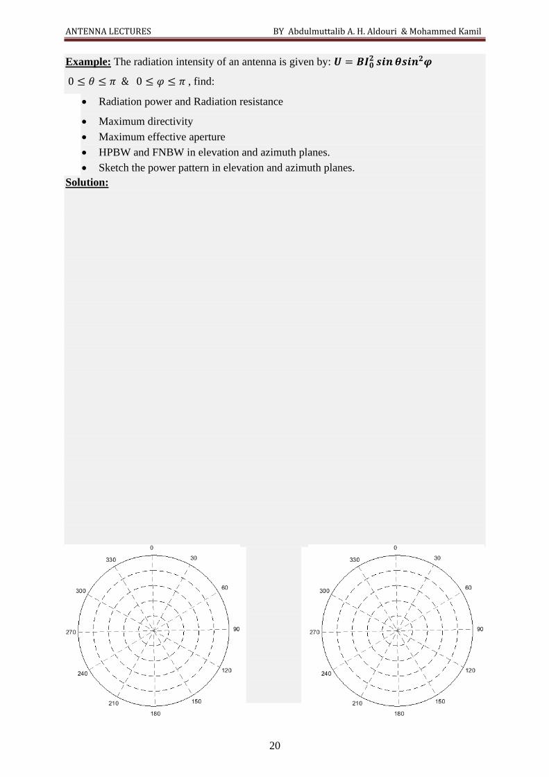
Example: The radiation intensity of an antenna is given by: 𝑼 = 𝑩𝑰𝟎𝟐 𝒔𝒊𝒏𝜽𝒔𝒊𝒏𝟐𝝋

0 ≤ 𝜃 ≤ 𝜋 & 0 ≤ 𝜑 ≤ 𝜋 , find:

• Radiation power and Radiation resistance

• Maximum directivity

• Maximum effective aperture

• HPBW and FNBW in elevation and azimuth planes.

• Sketch the power pattern in elevation and azimuth planes.

Solution:


21

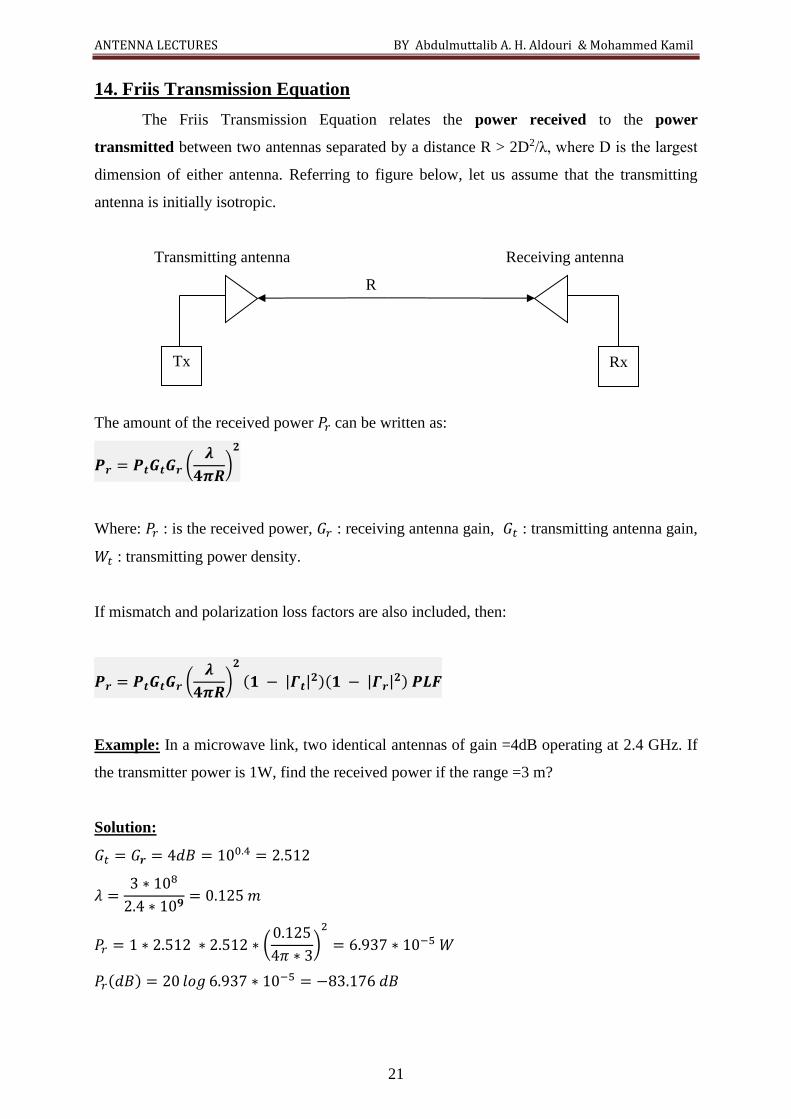
14. Friis Transmission Equation

The Friis Transmission Equation relates the power received to the power

transmitted between two antennas separated by a distance R > 2D2/λ, where D is the largest

dimension of either antenna. Referring to figure below, let us assume that the transmitting

antenna is initially isotropic.

Transmitting antenna Receiving antenna

R

The amount of the received power 𝑃𝑟 can be written as:

𝑷𝒓 = 𝑷𝒕𝑮𝒕𝑮𝒓 (𝝀

𝟒𝝅𝑹)𝟐

Where: 𝑃𝑟 : is the received power, 𝐺𝑟 : receiving antenna gain, 𝐺𝑡 : transmitting antenna gain,

𝑊𝑡 : transmitting power density.

If mismatch and polarization loss factors are also included, then:

𝑷𝒓 = 𝑷𝒕𝑮𝒕𝑮𝒓 (𝝀

𝟒𝝅𝑹)𝟐

(𝟏 − |𝜞𝒕|𝟐)(𝟏 − |𝜞𝒓|

𝟐) 𝑷𝑳𝑭

Example: In a microwave link, two identical antennas of gain =4dB operating at 2.4 GHz. If

the transmitter power is 1W, find the received power if the range =3 m?

Solution:

𝐺𝑡 = 𝐺𝒓 = 4𝑑𝐵 = 100.4 = 2.512

𝜆 =3 ∗ 108

2.4 ∗ 10𝟗= 0.125 𝑚

𝑃𝑟 = 1 ∗ 2.512 ∗ 2.512 ∗ (0.125

4𝜋 ∗ 3)2

= 6.937 ∗ 10−5 𝑊

𝑃𝑟(𝑑𝐵) = 20 𝑙𝑜𝑔 6.937 ∗ 10−5 = −83.176 𝑑𝐵

Rx Tx

Documents

ANTENNA LECTURES BY Abdulmuttalib A. H. …ceng.tu.edu.iq/eed/images/2019/CH1.pdfANTENNA LECTURES BY Abdulmuttalib A. H. Aldouri & Mohammed Kamil 4 1.2 Isotropic, Directional, and