arX

iv:1

108.

1916

v1 [

phys

ics.

ed-p

h] 9

Aug

201

1

Evaluation of inverse integral transforms for undergraduate

physics students

Aaron Farrell, Brandon P. van Zyl and Zachary MacDonald

Department of Physics, St. Francis Xavier University,

Antigonish, NS, Canada B2G 2W5

Abstract

We provide a simple approach for the evaluation of inverse integral transforms that does not

require any knowledge of complex analysis. The central idea behind the method is to reduce the

inverse transform to the solution of an ordinary differential equation. We illustrate the utility of the

approach by providing examples of the evaluation of transforms, without the use of tables. We also

demonstrate how the method may be used to obtain a general representation of a function in the

form of a series involving the Dirac-delta distribution and its derivatives, which has applications

in quantum mechanics, semi-classical, and nuclear physics.

1

I. INTRODUCTION

Integral transforms are usually presented to undergraduate physics majors well before

they are exposed to them in any rigorous fashion in their mathematics courses. The primary

motivation behind the integral transform is to re-write an ODE given in one representation

(the original t-domain), to another representation (the s-domain, or image domain) where

the solution is hopefully simpler; t and s are called conjugate variables. Once the solution

in the s-domain is known, the inverse transform is applied to obtain the desired solution in

the original t-representation. In this way, the integral transform is presented as yet another

tool to add to the arsenal of techniques that may be applied to find the solution of linear

ordinary differential equations.

The usefulness of the integral transform method for the solution of an ODE (or a set

of ODEs) is clearly predicated on the ability to perform the inverse transformation back

to the original domain. However, if the inverse transform requires complex contour inte-

gration methods (e.g., the inverse one-sided Laplace, two-sided Laplace, Mellin, and Weier-

strass transforms), most undergraduate physics students will find themselves at an impasse;

namely, students learning about methods for solving linear ODEs will likely have had no

exposure to complex analysis, and therefore, be unable to perform the inverse transforma-

tion without the use tables, or perhaps symbolic mathematics packages such as Maple c© or

Mathematica c©. If the inverse transform cannot be obtained, the student is left with no

choice but to attempt to solve the original problem using the set of techniques presented to

them in their course(s) on linear ordinary differential equations.

We wish to stress from the outset that the outcome of this tutorial does not change

the situation described above; that is, if the problem is to find the solution to an ODE

via an integral transform, and the inverse transform is not tabulated anywhere, then this

article will be of little help. Rather, we have in mind a scenario in which a particular

quantity of interest is explicitly formulated in terms of an inverse integral transform, and

where the evaluation of the inverse transform ostensibly requires the use of complex contour

integration methods. Our target demographic then, are undergraduate physics students with

no exposure to complex analysis, but already familiar with the solution of linear ordinary

differential equations.

To this end, the rest of our paper is organized as follows. In the next section, we provide a

2

brief overview of general linear integral transforms, from which we focus our attention to the

most common transforms arising in physics, where the inverse transform is a complex contour

integral. We then present some simple rules which may be applied to reduce the complex

contour integration problem to the solution of a linear ODE.1 In Sec. III, we illustrate

the method by providing several examples of inverse transforms involving complex contour

integrals, which are either not easily found in standard references, or not readily obtained

using symbolic mathematics packages. In all of our examples, the emphasis is on how to

find the inverse transform, and not technical mathematical details, which we are confident

will be covered in more formal mathematics courses. In Sec. IV, we demonstrate how our

approach may also be applied to obtain a multipole expansion of a function, which would

otherwise require a much more extensive mathematical analysis. Finally, in Sec. V we close

the tutorial with some concluding remarks.

II. INTEGRAL TRANSFORMS

We consider a generic integral transform of the form3

f(s) = I[F (t)] ≡∫ t2

t1

K(s, t)F (t)dt , (1)

where t ∈ R, K(s, t) is the kernel, and f(s) the image of F (t) under the transform I. The

inverse transform is given by

F (t) = I−1[f(s)] ≡∫ s2

s1

K−1(s, t)f(s) ds , (2)

such that

∫ s2

s1

K−1(s, t)K(s, t′)ds = δ(t− t′). (3)

Equation (3) may be used to determine the inverse Kernel, K−1(s, t) and, therefore whether

the parameter, s, is real or complex.

We now recall some properties of the integral transform. Linearity, I[F (t) + F (t)] =

I[F (t)] + I[G(t)], and multiplication by a constant I[AF (t)] = AI[F (t)] follow from the

integral definition of the transform given in Equation (1). Furthermore, it also follows

immediately from Eq. (1) that

3

sf(s) =

∫ t2

t1

(sK(s, t))F (t) dt; f (1)(s) =

∫ t2

t1

∂K

∂sF (t) dt, (4)

where the superscript in parenthesis denotes the order of the derivative with respect to the

argument of the function.

For the purposes of this paper, let us now focus on a class of Kernels (see also Sec. III C

below), given by

K(s, t) = Ceαst, α, C ∈ C (5)

which have the properties∂K

∂s= αtK , sK =

1

α

∂K

∂t. (6)

We thus observe that multiplication by s amounts to differentiating with respect to t and

derivatives with respect to s amount to multiplying by t. It is a straightforward exercise to

show that after n-fold applications of the multiplication and differentiation rules, we obtain

snf(s) =△n

αn+

(−1)n

αnI[F (n)(t)] , f (n)(s) = αnI[tnF (t)] , (7)

where

△n ≡[

n∑

m=1

(−1)m(sα)n−mesαtF (m−1)(t)]∣

∣

∣

t2

t1, (8)

are surface terms resulting from n-applications of integration by parts. Kernels of the type

in Eq. (5) also possess the so-called “shifting” property (let us take C = 1 for clarity),

f

(

s+A

α

)

=

∫ ∞

−∞eαst[eAtF (t)]dt = I[eAtF (t)] , (9)

and

e−Asf(s) =

∫ ∞

−∞eαste−AsF (t)dt =

∫ ∞

−∞eα(t−

A

α)sF (t)dt = I

[

F

(

t+A

α

)]

. (10)

In Table I, we present the various transforms that may be constructed by making par-

ticular choices for the parameters discussed above. Table II provides a summary of some of

the properties of integral transforms with Kernels of the form K(s, t) = Ceαst.

4

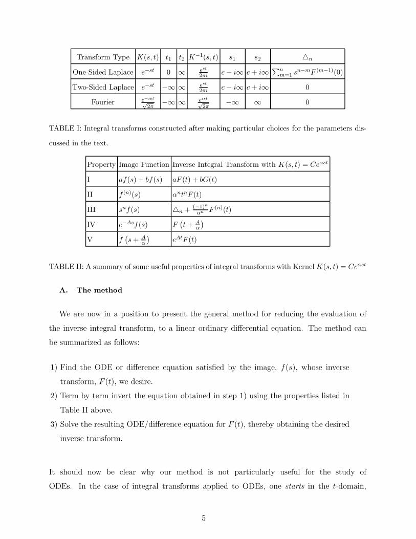
Transform Type K(s, t) t1 t2 K−1(s, t) s1 s2 △n

One-Sided Laplace e−st 0 ∞ est

2πi c− i∞ c+ i∞∑n

m=1 sn−mF (m−1)(0)

Two-Sided Laplace e−st −∞ ∞ est

2πi c− i∞ c+ i∞ 0

Fourier e−ist

√2π

−∞ ∞ eist√2π

−∞ ∞ 0

TABLE I: Integral transforms constructed after making particular choices for the parameters dis-

cussed in the text.

Property Image Function Inverse Integral Transform with K(s, t) = Ceαst

I af(s) + bf(s) aF (t) + bG(t)

II f (n)(s) αntnF (t)

III snf(s) △n + (−1)n

αn F (n)(t)

IV e−Asf(s) F(

t+ Aα

)

V f(

s+ Aα

)

eAtF (t)

TABLE II: A summary of some useful properties of integral transforms with Kernel K(s, t) = Ceαst

A. The method

We are now in a position to present the general method for reducing the evaluation of

the inverse integral transform, to a linear ordinary differential equation. The method can

be summarized as follows:

1) Find the ODE or difference equation satisfied by the image, f(s), whose inverse

transform, F (t), we desire.

2) Term by term invert the equation obtained in step 1) using the properties listed in

Table II above.

3) Solve the resulting ODE/difference equation for F (t), thereby obtaining the desired

inverse transform.

It should now be clear why our method is not particularly useful for the study of

ODEs. In the case of integral transforms applied to ODEs, one starts in the t-domain,

5

looking for the solution, F (t). The integral transform gives an algebraic equation for f(s),

which if solved, is followed by an application of the inverse transform to obtain F (t) in the

original domain. However, if we apply steps 1) and 2) above to f(s), the result will simply

be a restatement of the original ODE in the t-domain, which is of no help, given that it was

the ODE in the t-domain that motivated the transform to the s-domain in the first place.

Instead, our method is designed to reformulate a problem which may not be easily ac-

cessible to a student, e.g., finding the inverse transform via contour integration, to one for

which the student is already well equipped to handle — the solution of a linear ODE. We

are not suggesting that the solution of the resulting ODE will be simple (or even possible),

but rather, the key point is that the student will be empowered to find the inverse transform

using methods they are already comfortable, without having to rely solely on tables. In the

next section we present several applications of the method, which will serve to both clarify

its utility and applicability.

III. APPLICATIONS

A. Two-sided inverse Laplace Transform

From Table I, the two-sided Laplace transform (LT) is given by4

f(s) = B[F (t)] =∫ ∞

−∞e−stF (t) dt . (11)

It is assumed that the two-sided Laplace integral, Eq. (11), is convergent for Re s = c;

the question of whether or not the integral may be convergent for other values of s may be

answered by powerful theorems in Laplace transforms, which are not the focus of the present

tutorial.4 The inverse transform is given by

F (t) = B−1[f(s)] =1

2πi

∫ c+i∞

c−i∞estf(s) ds . (12)

The constant, c, must be greater than the largest real part of the zeros of the transform

function. Therefore, for the two-sided inverse Laplace transform (ILT), the contour may be

closed in either the left or right half plane, the choice being dependent on the function, F (t).

The two-sided LT may in fact be used as the basis for all of the integral transforms

presented in Table I. For example, if one puts s → is in Eq. (11), the Fourier transform

6

(FT) (aside from a constant) is immediately obtained.4 The one-sided LT is likewise simply a

special case of Eq. (11) provided we replace F (t) → F (t)Θ(t), where Θ(t) is the unit Heavisde

function. Moreover, the two-sided LT allows for the treatement of functions defined over

t ∈ R, in addition to loosening the restriction imposed by the FT, namely, that F (t) be

absolutely integrable over t ∈ R. It is also evident from Table I that the two-sided LT has

very simple operational rules; that is, △n = 0, whereas for the one-sided LT, △n 6= 0 and

requires a careful application to the term-by-term inversion of the ODE satisfied by f(s)

discussed above.

1. A few known results

To see the power of our approach in action, let us first demonstrate how to obtain some

well known ILTs4 by making use of the much simpler two-sided operational rules.

Example 1. Consider the following image

f(s) =1

sn+1, n ≥ 0 . (13)

The problem is to find the ILT of the image function, which by definition, requires the

calculus of residues. However, if we apply our three-step procedure outlined above, we find

that f(s) satisfies,

sf (1)(s) + (n+ 1)f(s) = 0 . (14)

Using the properties listed in Table II, we see that the ODE for F (t) is given by

− tF (1)(t) + nF (t) = 0 , (15)

which has the solution F (t) = Ctn. The constant C is determined by demanding that the

two-sided LT of F (t) (a real single variable integral) is identical to the image function f(s).

It is easy to see that we must have

F (t) = B−1

[

1

sn+1

]

=tn

Γ(n + 1)Θ(t) , (16)

which is a well known result from the one-sided ILT tables. Note that our simple two

sided operational rules naturally reproduce the one-sided results, and no complex contour

integration has been used.

7

Example 2. Next, consider the image function

f(s) = sn , n ≥ 0 , (17)

whose ILT we wish to find using our ODE method. The image function satisfies the following

first-order ODE,

sf (1)(s)− nf(s) = 0 . (18)

Applying the same approach as in the previous example, we find that F (t) satisfies

tF (1)(t) = −(n + 1)F (t) . (19)

Now, it is easy to show that F (t) = C/tn+1 (C is an integration constant) is a solution to

Equation (19). However,∫ ∞

−∞

e−st

tn+1dt , (20)

does not converge for any n ≥ 0. Therefore, while we have obtained a valid solution to

Eq. (19), it cannot be the two-sided ILT of f(s) since the forward transform, viz., Eq. (20)

does not exist. If F (t) cannot be given by the solution of a function, what is the other

possibility? As it happens, the only way to obtain a solution to Eq. (19), and have the

forward transform exist, is to extend the class of functions over which the two-sided LT is

defined to so-called tempered distributions.5 Tempered distributions are beyond the scope of

this tutorial, but fortunately, in the present case, the required distribution is the well-known

Dirac-delta distribution.

Using the fundamental properties for the derivative of the Dirac-delta distribution, we

observe that∫ ∞

−∞e−stδ(n)(t) dt = sn . (21)

We therefore conclude that

F (t) = B−1[sn] = δ(n)(t) . (22)

We note that Eq. (22) is also a solution to Eq. (19), but in the sense of a distribution,

meaning that both the left and right hand sides of Eq. (19) must be taken under an integral

sign, so that F (t) = δ(n)(t) acts on some arbitrary test function.

The message to be taken from this analysis is that the existence of the forward transform

must be ensured, over and above any formal solution to the ODE. This is a critical point,

8

as it serves to warn adopters of this method to be cautious in its application, since as we

have just seen, the function F (t) = C/tn+1, does not guarantee that the image, f(s), exists,

in spite of being a formal solution to Equation (19).

Example 3. Another useful, tabulated, image function is

f(s) = exp(−ns) , n ≥ 0 . (23)

The ODE satisfied by f(s) is given by

f (1)(s) + nf(s) = 0 , (24)

and the ODE statisfied by F (t) is therefore

− tF (t) + nF (t) = 0 . (25)

As in Example 2 above, the non-trivial solution to this equation can only be satisfied by the

Dirac-distribution, viz.,

F (t) = B−1[exp(−ns)] = δ(t− n) . (26)

Example 4. Our final example for this subsection is to find the two-sided ILT of

f(s) =e−k/s

s, k ≥ 0 . (27)

The ODE satisfied by f(s) is

s2f (1)(s) + sf(s)− kf(s) = 0 , (28)

which implies that F (t) satisfies

tF (2)(t) + F (1)(t) + kF (t) = 0 . (29)

It is an excellent exercise to show that the only acceptable solution to this second-order

ODE is

F (t) = J0(2√kt)Θ(t) . (30)

Once again, the simple two-sided operational rules have resulted in the correct one-sided

inverse Laplace transform.

9

2. A few lesser known results

Example 5. Consider

f(s) = exp(as3) , (31)

where a is a real positive constant. This image is rarely found in tables of ILTs, but it is

easily dealt with using our method. To wit, note that elementary differentiation yields

f (1)(s)− 3as2f(s) = 0 . (32)

The term by term ILT of Eq. (32) gives

F (2)(t) +1

3atF (t) = 0 . (33)

The solution to the above second-order ODE is well-known to be given by a linear combi-

nation of Airy functions,

F (t) = C1Ai

[ −t(3a)1/3

]

+ C2Bi

[ −t(3a)1/3

]

, (34)

where C1 and C2 are constants of integration. Since △n = 0 for the two-sided LT, we require

that

limt→±∞

e−stF (t) = 0 , (35)

from which we find that C2 = 0. The constant C1 is obtained by once again ensuring that

the forward transform yields Eq. (31), with the final result being given by

F (t) = B−1[exp(as3)] =1

(3a)1/3Ai

[ −t(3a)1/3

]

. (36)

Example 6. We now wish to find the ILT for the following images

fF (s) =πkBT

sin(πkBTs)= b csc bs , (37)

and

fB(s) = − πkBT

tan(πkBTs)= −b cot bs , (38)

where kB and T are constants, and b ≡ πkBT . Equations (37) and (38) have tremendous

importance in the formulation of quantum mechanics, semi-classical6 and nuclear physics7

10

at finite temperature, as will be discussed below. We begin with fF (s) and note that

csc(x− π) = − csc x , which allows us to write

fF

(

s− π

b

)

= −fF (s). (39)

We next multiply both sides of Eq. (39) by s− πbto obtain

(

s− π

b

)

fF

(

s− π

b

)

= −(

s− π

b

)

fF (s) , (40)

after which a term by term ILT yields

(etπ

b + 1)F(1)F (t) =

π

bFF (t) . (41)

The solution to Eq. (41) is formally given by

FF (t) = exp

(

π

b

∫

dt

etπ/b + 1)

)

. (42)

It is straightforward to show that

FF (t) =eC

e−tπ/b + 1=

eC

e−t/kBT + 1, (43)

where C is a constant of integration. We may fix C by appealing to final value theorem for

the LT, namely,4

limt→∞

F (t) = lims→0

sf(s) , (44)

which in the present case gives

eC = lims→0

bs

sin(bs)= 1 . (45)

Finally, it follows that

FF (t) = B−1

[

πkBT

sin(πkBTs)

]

=1

e−t/kBT + 1. (46)

We have only seen a similar form of Eq. (46) explicitly tabulated in one reference, where it

is simply stated without derivation.4

We now move onto

fB(s) = − πkBT

tan πkBTs. (47)

Making use of the fact that cot(x− π) = cot x, we readily obtain

fB

(

s− π

b

)

= fB(s) , (48)

11

which after multiplication on both sides by s− πbyields

(

s− π

b

)

fB

(

s− π

b

)

=(

s− π

b

)

fB(s). (49)

The term by term ILT of Eq. (49) gives

(etπ/b − 1)F(1)B (t) = −π

bFB(t) . (50)

Analogous to the treatment of FF (t) above, the solution to this ODE is given by

FB(t) = C exp

(

π

b

∫

dt

1− etπ/b

)

=C

e−t/kBT − 1. (51)

Another application of the final value theorem shows that C = 1 and therefore4

FB(t) = B−1

[

− πkBT

tan(πkBTs)

]

=1

e−t/kBT − 1. (52)

3. Physical Application: Ideal harmonically trapped quantum gases at finite temperature

An immediate application of the inverse transforms derived above are harmonically

trapped, ideal quantum gases at finite temperature. A self-contained discussion of the

physics of these systems is well beyond the scope of this article, so here, we wish to simply

provide the basic mathematical tools, and introduce how the method we have proposed can

be used to introduce a complementary formulation of quantum systems, that is not widely

known to many physicists. The interested reader is encouraged to examine Refs. [6,8,9] and

the references therein for more details.

The central theoretical tool from which all thermodynamic properties of the ideal gas can

be derived is the Bloch density matrix (BDM). At zero temperature, the BDM is given by

C0(r, r′; s) =

∑

all i

ψ⋆i (r)ψi(r

′) exp(−sǫi) , (53)

where the ψi’s and the one-particle energies ǫi are the solutions to the time-independent

Schrodinger equation, and the quantity, s, is a complex variable. The BDM appears to

require the explicit single-particle wave functions for its evaluation, but in fact, this is not

always the case. The BDM satisfies the Bloch equation

HrC0(r, r′; s) = −∂C0(r, r

′; s)

∂s, (54)

12

where Hr is the Hamiltonian and C0(r, r′; s) is subject to the initial condition

C0(r, r′; s = 0) = δ(r− r′) . (55)

Therefore, an explicit form for C0 is, at least in principle, possible once the external potential

is defined, and used in the Hamiltonian, Hr, to solve Equation (54).

In the present application, we will take the external confinement to be a three-dimensional

isotropic harmonic oscillator, V (r) = 12mω2

0r2, with r =

√

x2 + y2 + z2, and ω0 the trapping

frequency. Under such a confining potential, the exact zero temperature BDM is found to

be given by8

C0(r, r′; s) =

(

1

2π sinh(s)

)3/2

exp

[

−(

r+ r′

2

)2

tanh(s/2)−(

r− r′

2

)2

coth(s/2)

]

. (56)

The zero temperature BDM is independent of the quantum statistics of the particles, mean-

ing that we have a unified treatment for either Fermi or Bose gases (including Bose-Einstein

Condensation). Using Eq. (56), we may obtain the finite temperature first-order density

matrix (FDM) via a two-sided ILT,6,8,9

ρ(r, r′;T ) = B−1µ

[g

sCT (r, r

′; s)]

, (57)

where

CT (r, r′; s) = C0(r, r

′; s)πskBT

sin(πskBT )(fermions) ,

= −C0(r, r′; s)

πskBT

tan(πskBT )(bosons) , (58)

and now kB and T take on the physical significance of the Boltzmann constant and tem-

perature, respectively. Note that in Eq. (57), we have introduced the subscript, µ, in the

two-sided ILT to emphasize that the conjugate variable to s in this problem is µ, the chemical

potential. The factor, g in Eq. (57) depends on the spins of the particles through g = 2s1+1,

where s1 is the spin of the particle. For spin-1/2 fermions, g = 2, and for spinless bosons,

g = 1. The finite temperature BDM, CT , encodes the quantum statistics by appropriately

weighting the zero temperature Bloch density matrix. It should now be evident why we

must utilize the two-sided ILT, rather than the one-sided ILT; the chemical potential, µ,

must be allowed to take on both positive and negative values at finite temperature, whereas

the one-sided ILT only allows for µ ≥ 0.

13

Equation (57) is the fundamental quantity from which all of the thermodynamic proper-

ties of the trapped gases (fermions or bosons) may be investigated. For example, the finite

temperature spatial density, ρ(r;T ) is immediately obtained by putting r = r′ in Eq. (57),

while the the finite temperature kinetic energy density can be found from

τ(r;T ) =

3∑

i=1

[

∂2

∂xi∂x′iρ(r, r′;T )

]

. (59)

Following the calculations in Ref. [9], the ILTs we have presented earlier may be used to

explicitly evaluate ρ(r, r′;T ).

In the case where the potential, V (r), is such that an exact, closed form expression for

C0(r, r′; s) is not possible, an ~-expansion may be performed, viz.,

C0(r, r′; s) =

(

1

λ

)3

e−sV (r)e−m(r−r

′)2

2~2s

(

1− ~2s2

12m

[

∇2V − s

2(∇V )2

]

+ · · ·)

, (60)

where for economy of space, we have only shown terms up to relative order ~2, λ ≡(2π~2s/m)1/2 and ~ is Planck’s constant divided by 2π. Equation (60) is called the semi-

classical expansion of the BDM, and the higher order ~-terms, containing gradients of the

potential, represent quantum corrections to the classical result. The semi-classical expansion

may be used as the foundation for the study of quantum effects in a variety of systems by

systematically introducing higher-order quantum corrections and examing their influence on

the physical properties of the system. A detailed discussion of the applications of Eq. (60)

in semi-classical physics may be found in Reference [6].

B. Inverse Fourier transform

The inverse Fourier transform (IFT) is mathematically much easier than the ILT, since

the IFT is an integral over the real line. Nevertheless, it is worthwhile illustrating our

method as it applies to the IFT, particularly in cases where standard approaches to finding

the inverse transform require some “tricks” for its evaluation.

Example 7. Let us then consider the following image

f(s) =

√

π

σe

−s2

4σ . (61)

14

Simple differentiation shows that

f (1)(s) =

(√

π

σe

−s2

4σ

)

(

− s

2σ

)

= − s

2σf(s) , (62)

and thus f(s) satisfies the following first order differential equation

f (1)(s) +s

2σf(s) = 0 . (63)

Applying the properties in Table II to Eq. (63) above leads to the following ODE for F (t)

F (1)(t) + 2σtF (t) = 0 . (64)

Obtaining the solution to Eq. (64) is elementary, and is given by

F (t) = Ce−σt2 . (65)

The constant C is adjusted such that the Fourier transform of F (t) is f(s). It then follows

that

F (t) = F−1

[√

π

σe

−s2

4σ

]

= e−σt2 . (66)

Obtaining Eq. (66) using standard techniques is more involved.10

C. Mellin transform

The Mellin transform (MT) may also be treated by the ODE method presented here.

The Mellin transform is defined by11

f(s) = M[F (t)] =

∫ ∞

0

ts−1F (t) dt , (67)

and its inverse is given by

F (t) = M−1[f(s)] =1

2πi

∫ c+i∞

c−i∞t−sf(s) ds . (68)

Once again, we observe that the two-sided LT may be viewed as the fundamental tool for

our operational calculus, since the MT may also be obtained from to the two-sided LT by

noting that4

M[F (t)] = B[F (e−t)] . (69)

15

The only thing left to do is to determine the corresponding “rules” as we did for transforms

with exponential kernels. It is straightforward to confirm that following rules are obeyed for

the Mellin transform:

M[F (at)] = a−sf(s)

M[taF (t)] = f(s+ a)

M[F (1)(t)] = −(s− 1)f(s− 1)

M[tnF (n)(t)] = (−1)nΓ(n+ s)

Γ(s)f(s) . (70)

Example 8. To illustrate the method applied to the MT, let us use it to evaluate the

complex contour integral,1

2πi

∫ c+i∞

c−i∞t−sΓ(s) ds , (71)

which we recognize as the inverse Mellin transform of f(s) = Γ(s). According to the rules

given above, we note that

f(s+ 1) = sf(s) . (72)

Applying the inverse rules to Eq. (72) yields

F (1)(t) = −F (t) , (73)

which is immediately seen to to have the solution

F (t) = Ce−t . (74)

The constant, C, is found by ensuring that the forward transform, f(s) = Γ(s) (which is just

a real integral), is obtained, which gives C = 1. Therefore, we have evaluated the complex

contour integral,

e−t =1

2πi

∫ c+i∞

c−i∞t−sΓ(s) ds , (75)

using only elementary methods.

IV. MULTIPOLE EXPANSIONS OF FUNCTIONS

In this section, we wish to illustrate how to obtain the “multipole” expansion of a func-

tion, F (t), in the form of a series involving the Dirac-delta distribution and its derivatives.

16

Such expansions have been found to be useful in semi-classical physics, where they may be

used to introduce quantum corrections,12–14 and in nuclear physics, for the calculation of

approximate wave functions for realistic nuclear potentials.15

The method presented here is general, and uses a very simple approach based on the two-

sided inverse Laplace transform. An immediate benefit of our formulation is that it permits

an easy determination of all of the moments of a function, F (t) (see Eq. (79) below). In

addition, our approach allows us to obtain results that have previously required intense

mathematical analysis and dedicated papers for their derivation.

In the most generic of cases, we begin with the forward two-sided LT of F (t), viz.,

f(s) =

∫ ∞

−∞e−stF (t)dt . (76)

Assuming that f(s) is analytic, we use the series expansion, e−st =∑∞

n=0(−1)nsntn/n!, in

Eq. (76) to obtain

f(s) =∞∑

n=0

(

(−1)n

n!

∫ ∞

−∞tnF (t)dt

)

sn. (77)

At this point, we are not worrying about the fact that we have taken the summation outside

of the integral, since our end result will be an expansion that is defined only in the sense

of a distribution, and therefore will only be valid under the integral sign. We now term by

term Laplace invert Eq. (77), which yields

F (t) =

∞∑

n=0

(−1)n

n!Inδ

(n)(t) , (78)

where

In =

∫ ∞

−∞qnF (q) dq , (79)

is the n-th moment of the function, F (t). The n = 0 term is sometimes referred to as the

the “monopole” moment, and the n = 1 the “dipole” moment, and so on. Equation (78) is

the general form of the multipole moment expansion, and is to be viewed in the distribution

sense, having meaning only under the integral sign.

Example 9. In most practical applications, the moments of the function, Eq. (79),

need not be explicitly calculated. To see this, let us first consider F (t) = Ai(t). We can

deduce from Eq. (36) that,

f(s) = exp

(−s33

)

, (80)

17

is the two-sided LT of F (t). We then formaly write f(s) as a series expansion,

exp

(−s33

)

=

∞∑

n=0

(−1)ns3n

3nn!, (81)

and then term by term ILT both sides of Eq. (81) (with the aid of Example 2) to obtain

Ai(t) = B−1

[ ∞∑

n=0

(−1)ns3n

3nn!

]

=

∞∑

n=0

(−1)nδ(3n)(t)

3nn!. (82)

A comparison of Eq. (79) with Eq. (82) may be used to determine the moments of the Airy

function. Equation (82) has been derived earlier by several authors,12–14 but by using a

much more involved approach than the one presented here. As commented above, it is im-

portant to remember that Eq. (82) is to be interpreted strictly in the sense of a distribution.

Example 10. Next we find an analogous expansion for the Bessel function,

F (t) = Jν(ωt)Θ(t), where Re [ν] > −1. The well known Laplace transform of this

function is16

f(s) = B[Jν(ωt)Θ(t)] =

(√ω2 + s2 − s

)ν

ων√ω2 + s2

. (83)

As in the previous example, we consider a formal series expansion of f(s),

(√ω2 + s2 − s

)ν

ων√ω2 + s2

=

∞∑

n=0

2nΓ(

n+1−ν2

)

sn

n!Γ(−ν−n+1

2

)

ωn+1, (84)

followed by a term by term two-sided ILT of both sides of Equation (84). The result of this

inversion is

Jν(ωt)Θ(t) =∞∑

n=0

2nΓ(

n+1−ν2

)

δ(n)(t)

n!Γ(−ν−n+1

2

)

ωn+1. (85)

To our knowledge, Eq. (85) is a new result, and its use can immediately be seen from an

examination of integrals for the form

I(ν) =

∫ ∞

0

ϕ(r)Jν(r) dr

=

∞∑

n=0

(−1)n2n−1Γ

(

n+1−ν2

)

ϕ(n)(0)

n!Γ(−ν−n+1

2

) . (86)

Again, a comparison of Eq. (79) with Eq. (85) allows us to obtain all of the moments of Jν ,

viz.,

In = (−1)n2nΓ

(

n+1−ν2

)

Γ(−ν−n+1

2

)

ωn+1, (87)

18

which by direct application of Eq. (79) would have been more difficult.

Example 11. As our final example, we consider the multipole expansion of the Fermi

function,15

F (t) =1

[e(t−R)/a + 1]. (88)

In nuclear physics applications, R would denote the nuclear radius, and a the “diffuseness”

of its surface. It is straightforward to deduce from Eq. (46), and property IV of Table II,

that F (t) has the image

f(s) = − πa

sin(πas)e−Rs . (89)

We next expand f(s) as a power series about the diffuseness parameter, a, and obtain the

expansion

− πa

sin(πas)e−Rs = −e

−Rs

s−

∞∑

k=0

A2k+1a2k+2e−Rss2k+1 , (90)

where

A2k+1 =2(22k+1 − 1)π2k+2

(2k + 2)!|B2k+2| , (91)

and the B2k+2 are the known Bernoulli numbers. The term by term two-sided ILT of Eq. (90)

gives1

[e(t−R)/a + 1]= Θ(R− t)−

∞∑

k=0

A2k+1a2k+2δ(2k+1)(t− R) . (92)

Equation (92), which we have derived in only a few lines, has previously been the focus of

an entire paper by L. Lukyanov,15 thereby emphasizing just how useful the approach we

present here can be in a wide array of problems. In fact, what is remarkable is just how

trivial Eq. (92) was to obtain when compared to the analysis presented in Reference [15].

V. CLOSING REMARKS

We have presented an alternative approach for the evaluation of common inverse trans-

forms occurring in physics without having to introduce complex contour integration. Our

operational calculus has been based on the two-sided Laplace transform, which has allowed

us to examine a much wider class of functions than would be possible using other trans-

forms. We have also highlighted the power of the two-sided inverse Laplace transform by

19

demonstrating how it can often make trivial work of problems (e.g., Examples 9 and 11),

which otherwise require a much more extensive analysis.

Some may find the presentation in this tutorial lacking in mathematical rigor. In partic-

ular, we have purposefully avoided technical discussions of strips of convergence, for which

at best, the integral transform is valid. For the examples we have provided, where the strip

of convergence is not indicated, the latter has to be investigated, given the original F (t),

for each individual case separately. Indeed, a useful exercise to give to students would be to

determine the strips of convergence for each of the examples provided in this paper.

Nevertheless, it is important to keep in mind that in undergraduate physics culture,

advanced mathematical tools (e.g., integral transforms) are often needed right away — stu-

dents just need to know how to use the tools, with the details of all the theorems and proofs

being covered in more formal mathematics courses. Therefore, we hope the techniques pre-

sented in this tutorial will also find their way into the physics classroom, where they may be

used to enable students to evaluate integral transforms with confidence, and without being

slaves to tables. We also hope that our presentation will inspire students to further examine

the formulations of quantum mechanics, semi-classical physics,6 and density-functional the-

ory,6,17 all of which may be based on the two-sided Laplace transform. Finally, we believe

that our general results for the multipole expansion of functions will be of interest to prac-

ticing physicists, particularly those involved in the foundations of quantum, semi-classical

and nuclear physics research.

VI. ACKNOWLEDGEMENTS

Z. MacDonald would like to acknowledge the Natural Sciences and Engineering Research

Council of Canada (NSERC) USRA program for financial support. B. P. van Zyl and A.

Farrell would also like to acknowledge the NSERC Discovery Grant program for additional

financial support.

1 After the completion of this work, we became aware of a long forgotten paper (Ref. [2]) in

which a similar idea is proposed. However, Ref. [2] focuses soley on the one-sided ILT, which

amounts to a special case of the present paper. Indeed, our presentation is applicable to a

20

wider array of functions, has simpler operational rules, and thereby allows us to present new

results (e.g., the multipole expansions presented in Examples 9–11, which in our opinion, are

publishable results in their own right) which would not be possible using the method presented

in Reference [2]. Regardless, given that the approach presented in this tutorial is not discussed

in any undergraduate textbooks we are aware of, it is certainly worthy of presenting to a broader

audience.

2 H. Goldenberg, SIAM Review, 4, 94 (1962).

3 G. B. Arfken and H. J. Weber, Mathematical Methods For Physicists, 6th ed. (Elseveir Academic

Press, Burlington, MA, 2005).

4 B. van der Pol and H. Bremmer, Operational Calculus Based on the Two-sided Laplace Integral,

3rd ed. (Chelsea Publishing Company, New York, New York,1987)

5 I. M. Gel’fand and G. E. Shilov, Generalized Functions. (Academic Press Inc., 1964).

6 M. Brack and R. K. Bhaduri, Semiclassical Physics, Frontiers in Physics, Vol. 96 (Addison-

Wesley, Reading, MA, 2003).

7 P. Ring and P. Schuck, The Nuclear Many-Body Problem, (Springer-Verlag, Berlin, Germany,

2004).

8 B. P. van Zyl, R. K. Bhaduri, A. Suzuki, and M. Brack, Phys. Rev. A 67, 023609 (2003).

9 B. P. van Zyl, Phys. Rev. A 68, 033601 (2003).

10 see, e.g., Problem 2.22 in D. J. Griffiths, Introduction to Quantum Mechanics, 2nd ed., (Pearson

Education, Inc. , Upper Saddle River, NJ, 2005)

11 E. C. Titchmarsh, Introduction to the Theory of Fourier Integrals, 2nd ed., (Oxford University

Press, New York, 1937).

12 G. P. Arrighini, N Durante, and C. Guidotti, J. Math. Chem. 25, 93 (2005).

13 E. J. Heller, J. Chem. Phys. 68, 2066 (1978).

14 B. Hupper and B. Eckardt, Phys. Rev. A 57, 1536 (1998).

15 V. K. Lukyanov, J. Phys. G: Nucl. Part. Phys. 21, 145 (1995).

16 I. S. Gradshteyn and I. M. Ryzhik, Table of integrals, series, and products, 4th ed (Academic

Press Inc,, New York, New York, 1980).

17 B. P. van Zyl, K. Berkane, K. Bencheikh, and A. Farrell, Phys. Rev. B 83, 195136 (2011).

21