Embed Size (px)
Citation preview
Appendix A: Stereographic Projection
Not too many years ago all students who were introduced to crystallography, even if they were not intending to study it in any great depth, were started off with a few laboratory exercises in the use of stereographic projections. In recent years there seems to have been a tendency to neglect this topic, which is unfortunate, because a knowledge of the techniques of drawing and interpreting stereographic projections is extremely useful.
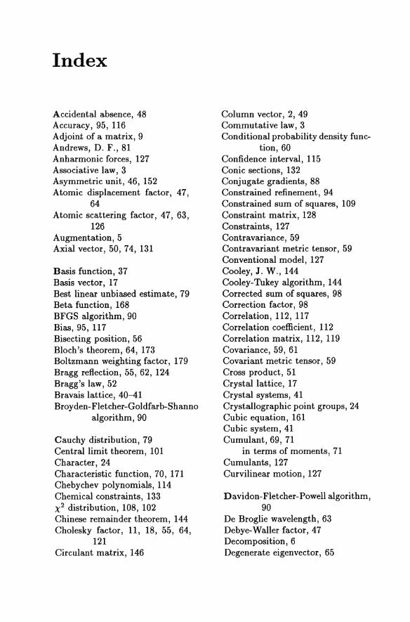
The normals to planes in a crystal, whether they are natural faces or invisible reflecting planes, may be projected onto the surface of a sphere by locating the crystal at the center of the sphere, drawing radial lines perpendicular to the planes, and marking the points at which they intersect the surface. Referring to Figure A.I, the points marked on the surface ofthe sphere may be represented on a plane sheet of paper by drawing a line from the point to the opposite pole of the sphere, and marking the intersection of this line with the equatorial plane. All points on the upper hemisphere may thus be plotted inside the equatorial circle. We represent an actual crystal in projection by considering that the polar axis of our sphere is perpendicular to our paper. Meridians of longitude are then represented by radial lines in the circle.
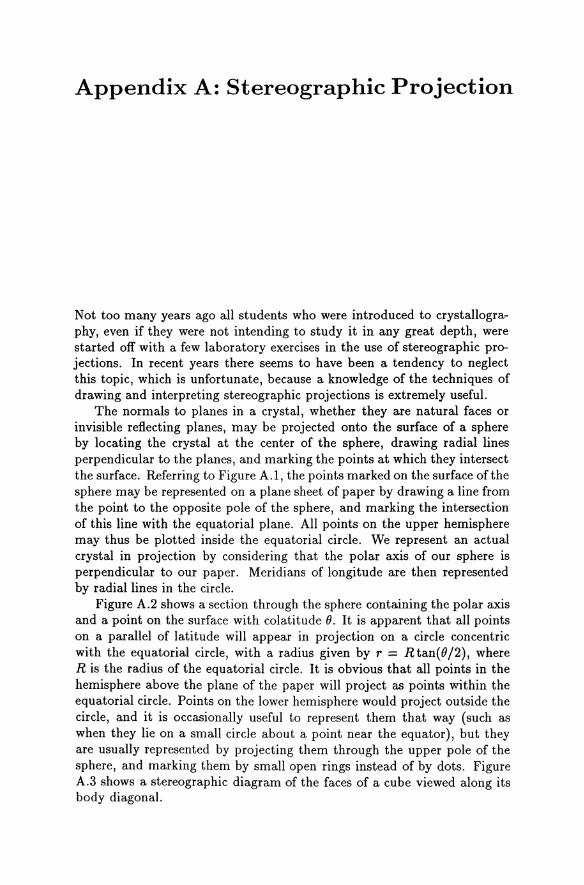
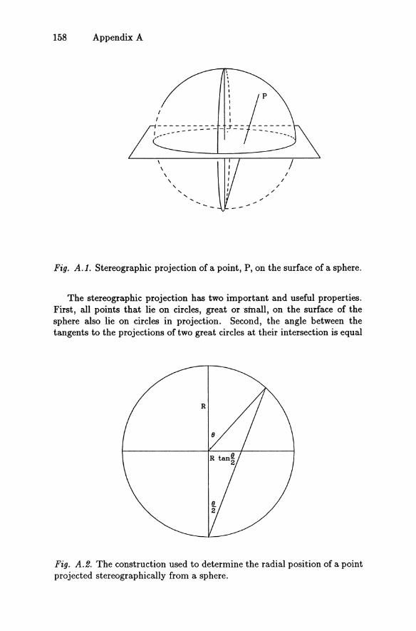
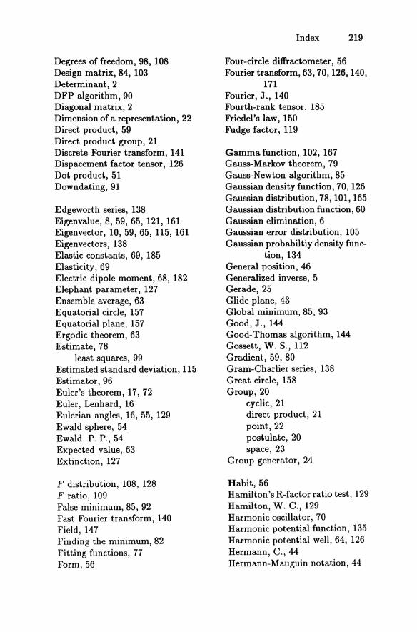
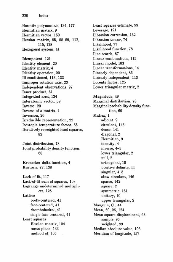
Figure A.2 shows a section through the sphere containing the polar axis and a point on the surface with colatitude (). It is apparent that all points on a parallel of latitude will appear in projection on a circle concentric with the equatorial circle, with a radius given by r = Rtan((}/2), where R is the radius of the equatorial circle. It is obvious that all points in the hemisphere above the plane of the paper will project as points within the equatorial circle. Points on the lower hemisphere would project outside the circle, and it is occasionally useful to represent them that way (such as when they lie on a small circle about a point near the equator), but they are usually represented by projecting them through the upper pole of the sphere, and marking them by small open rings instead of by dots. Figure A.3 shows a stereographic diagram of the faces of a cube viewed along its body diagonal.
158 Appendix A
, I I I
I 1 I \ JP ---------- J-- -------
1 •• -- - - - - - - - - - - • - - - - - - - - ___ •
/' /'
/
/ /
Fig. A.1. Stereographic projection of a point, P, on the surface of a sphere.
The stereographic projection has two important and useful properties. First, all points that lie on circles, great or small, on the surface of the sphere also lie on circles in projection. Second, the angle between the tangents to the projections of two great circles at their intersection is equal
Fig. A.2. The construction used to determine the radial position of a point projected stereographically from a sphere.
Stereographic Projection 159
•
o
•
Fig. A.3. A stereographic projection of the faces of a cube, as seen looking down the body diagonal.
to the dihedral angle between the planes of the great circles, irrespective of where in the projection the intersection occurs. Thus, the pattern of the projections of circles that intersect in a symmetry axis reflects the symmetry
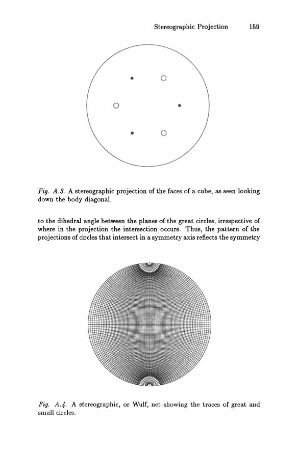
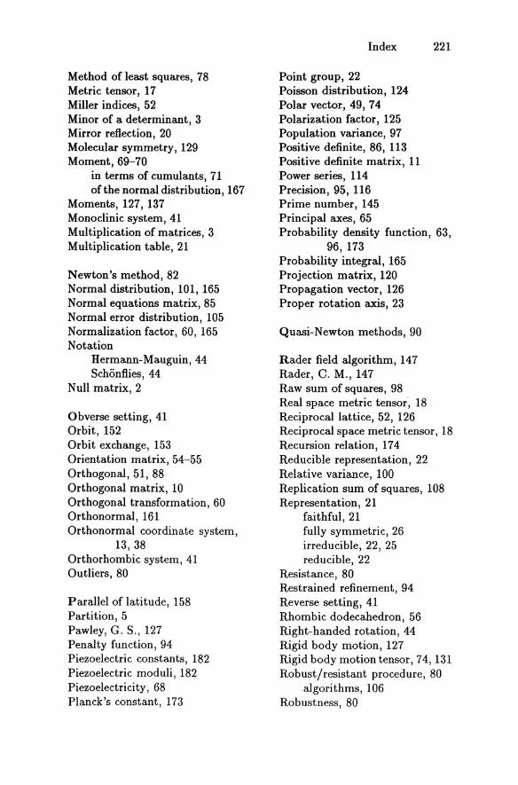
Fig. A.4. A stereographic, or Wulf, net showing the traces of great and small circles.
160 Appendix A
of the axis. In practical applications of stereographic projection it is useful to have
a chart of the projected traces of parallels of latitude and meridians of longitude, with the poles at the top and bottom, a so-called Wulf net. Wulf nets may be obtained from various commercial suppliers, or, in this era of computer driven plotters, one may be produced with a relatively trivial program. Figure A.4 is an example of such a chart. I have one that is ten inches in diameter, mounted on a drawing board with a thumb tack sticking up through the middle. (It is important not to put your hand down on the point of the tack!) A sheet of translucent paper is laid on top of it, with the tack sticking through so that the paper may be rotated about the center. The radial coordinate represents the angle of a full circle goniometer, and the angular coordinate represents the angle. Reflections found in a systematic search on a diffractometer are plotted on the paper. The angle between the normals of two sets of planes is found by rotating the paper so that the projections of both normals fall on the same meridian, and then counting the parallels between them. Prominent zones lie on great circles, and the angles between zones identify the symmetry of the axis that is perpendicular to both zone axes. Such a plot can be of immense help in determining the orientation of an unknown crystal.
Appendix B: Eigenvalues and Eigenvectors of 3 x 3 Symmetric Matrices
The determination of eigenvalues and eigenvectors of symmetric matrices in three dimensional space requires the solution of the secular equation IA - All = O. This is a cubic equation of the form A3 + aA2 + bA + c = 0, where
a -(A11 + A22 + A 33 ),
b (A11A22 - AI2) + (AllA33 - AI3) + (A22A33 - A~3)' and
c -(AllAnA33 + 2Al2Al3A23 - AllA~3 - AnAI3 - A33A I2)·
Although it is rarely discussed in standard algebra courses, there is a direct algorithm for the analytic solution of cubic equations. The first step is to make the substitution A = x - a/3, which eliminates the coefficient of the quadratic term, and leaves an equation of the form x 3 - qx - r = 0, where q = a2 /3 - b, and r = -(2a3 /27 - ab/3 + c). If the matrix is symmetric, the equation must have three real roots, meaning that 27r2 must be less than 4q3. We find the smallest positive angle <p = arccos[J27r2 /4q3], and the three eigenvalues are then Al = C cos (<p/3) - a/3, A2 = C cos[(21r -<p)/3]- a/3, and A3 = C cos [(271" + <p)/3]- a/3, where C = J4q/3.
When the three eigenvalues have been determined, the eigenvectors may be found by substituting the eigenvalues into the system of equations Au = AU. However, because the matrix (A - AI) is singular when A is an eigenvalue, only two of the three equations are independent. The third condition is supplied by requiring that the coordinate system defined by the three eigenvectors be orthonormal. Let Uli, U2i and U3i be the direction cosines of the eigenvector corresponding to the eigenvalue Ai, with respect to the coordinate system in which A is defined. We then have 111 + U~i + U~i = 1. Let Xl and X2 be uI;ju3i and u2;ju3i, respectively. (This assumes that U3i i- O. If two of the off-diagonal elements in any row and column of A are equal to zero, then one of the coordinate axes is an
162 Appendix B
eigenvector, and the problem reduces to a quadratic.) The basic equations can then be written
The solutions are
(All - Adxl + A 12 X2
A 12 Xl + (A22 - Ai)X2
Xl [-A13(A22 - Ad + A 12 A 23]/.to.,
X2 [-A23(Au - Ai) + A 12 A 13]/.to.,
where .to. = [(All - Ai)(A22 - Ai) - AI2j. The direction cosines are then
Uli = xdD, U2i = xdD, and U3i = liD,
where D = J xi + x~ + l. If the elements of an anisotropic displacement factor tensor, {3, have
been determined by least squares refinement, this procedure enables us to compute the directions and magnitudes of the principal axes of the thermal ellipsoid. We would also like to know something about the precision with which we have determined these amplitudes. We will have determined the variance-covariance matrix for the six independent tensor elements, {3ij. Denote this 6 x 6 matrix by Y. We need the vector of derivatives, D, whose elements are Di = fJAi/fJ{3jk. Then the variance of A, at is given by O"~ = DTYD. The expressions for the derivatives, D i , are complicated, but each step in the determination of A expresses a set of derived quantities as an analytic function of previously derived quantities, so that the required derivatives can be readily represented by a matrix product in which the elements of each matrix are the derivatives of derived quantities with respect to the quantities derived in the previous step.
Appendix C: Sublattices and Superlattices
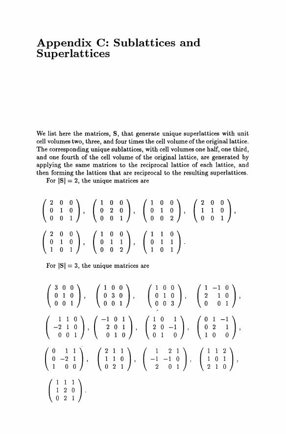
We list here the matrices, S, that generate unique superlattices with unit cell volumes two, three, and four times the cell volume of the original lattice. The corresponding unique sublattices, with cell volumes one half, one third, and one fourth of the cell volume of the original lattice, are generated by applying the same matrices to the reciprocal lattice of each lattice, and then forming the lattices that are reciprocal to the resulting superlattices.
For lSI = 2, the unique matrices are
u 0 n, 0 0 0,0 0
0' ( 2 0 n, 1 2 1 1 1
0 0 0 0 0
U 0 0, U 0 D, 0 1 n 1 1 1
0 0 0
For lSI = 3, the unique matrices are
COO ) COO ) U 0 n, u -I 0) o 1 0 , o 3 0 , 1 1 0 ,
001 001 0 o 1
( 1 1 0 ) CI 0 I) C 0 I) C 1 -I ) -2 1 0 , 2 0 1 , 2 0 -1 , 0 2 1 , 001 o 1 0 0 1 o 1 0 0 ell ) CI D' (
1 2 1 ),0 1 2) o -2 1 , 1 1 -1 -1 0 o 1 , 1 0 0 o 2 2 0 1 1 0
U 1
D 2 2
164 Appendix C
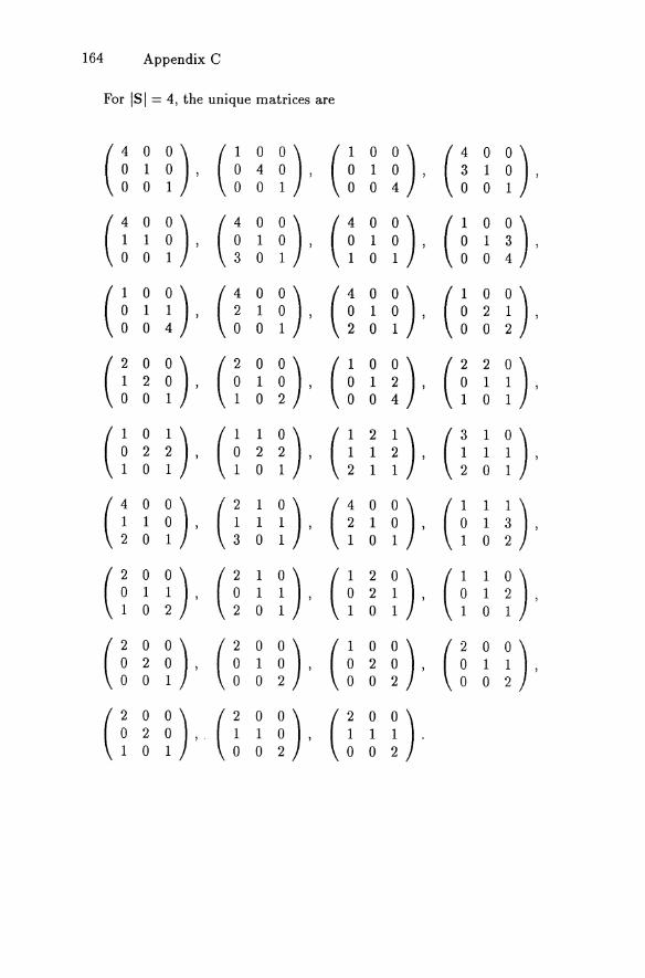
For IS I = 4, the unique matrices are
U 0
D' U 0 n, u 0
0' U 0 n 1 4 1 1 0 0 0 0
(! 0 n, (: 0 n, 0 0
D' U 0 n, 1 1 1 1 0 0 0 0
U 0
D' U 0 D, 0 0
D' U 0 !) 1 1 1 2
0 0 0 0
U 0
D' (! 0 n, u 0
D' (: 2 n 2 1 1 1 0 0 0 0
0 0
D'O 1
D' (l 2 D, (: 1 n, 2 2 1 1 0 0 1 0
(l 0 D,(l 1 :), (l 0
D' 0 1
D 1 1 1 1 0 0 0 0
U 0 !), (: 10) 0 2
D' 0 1 n, 1 1 1 , 2 1 0 0 1 0 0
U 0
D' U 0 n, u 0 n, u 0
D' 2 1 2 1 0 0 0 0
(: 0
D' U 0 D,n 0 D 2 1 1
0 0 0
Appendix D: The Probability Integral, The Gamma Function, and Related Topics
We have made extensive use of probability density functions that included normalization factors, N, such that
1+00 (liN) -00 f(x)dx = 1.
In most cases we have stated without proof what these factors are, but in many cases it is useful to have some idea of their approximate magnitudes. The most frequently encountered of these is the normalization factor for the normal, or Gaussian, distribution. To determine this we need to evaluate the so-called probability integral,
1+00 P = -00 exp (_x 2 12) dx.
Consider first the surface integral
and also the corresponding function in polar coordinates
1+71' 1+00 dB r exp( _r2 12)dr.
-71' 0
Because the integrand is everywhere positive, we can write inequalities (see
166 Appendix D
y
L-------------------~------~--x
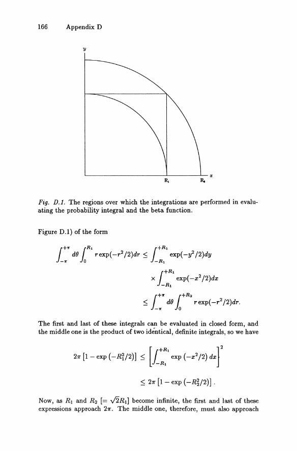
Fig. D.l. The regions over which the integrations are performed in evaluating the probability integral and the beta function.
Figure D.1) of the form
1 +11" {R' 1+R, -11" de Jo r exp( _r2 /2)dr::; -R, exp(-y2/2)dy
1+R , x exp( _x 2 /2)dx
-R,
1 +11" 1+R2 ::; -11" de 0 rexp( _r2 /2)dr.
The first and last of these integrals can be evaluated in closed form, and the middle one is the product of two identical, definite integrals, so we have
::; 27r [1- exp (-RV2)] .
Now, as Rl and R2 [= v'2R1] become infinite, the first and last of these expressions approach 27r. The middle one, therefore, must also approach
The Probability Integral and Related Topics 167
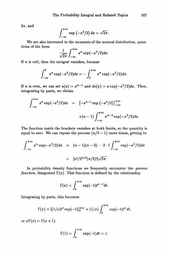
211", and 1:00 exp (_x 2 /2) dx = y'2;.
We are also interested in the moments of the normal distribution, quantities of the form
~ 1+00 xn exp( _x2 /2)dx. v 211" -00
If n is odd, then the integral vanishes, because
10 1+00 xn exp( _x2 /2)dx = - xn exp( _x2 /2)dx.
-00 0
If n is even, we can set u(x) = xn- 1 and dv(x) = xexp(-x2/2)dx. Then, integrating by parts, we obtain
1+00
-00 xn exp( _x2 /2)dx =
The function inside the brackets vanishes at both limits, so the quantity is equal to zero. We can repeat the process (n/2 - 1) more times, getting to
1:00 xn exp( _x2 /2)dx = (n - 1)(n - 3)···3·1 1: exp( _x2 /2)dx
[n!/2n/2(n/2)!]~
In probability density functions we frequently encounter the gamma
function, designated r(x). This function is defined by the relationship
[+00 r(x) = Jo exp( -t)tX-ldt.
Integrating by parts, this becomes
[+00 r(x) = [(1/x)tXexp(-t)]too + (1/x) Jo exp(-t)tXdt,
or xr(x) = r(x + 1).
[+00 r(1) = Jo exp(-t)dt = 1.
168 Appendix D
It follows from these two relationships that f(n) = (n - 1)! when n is a positive integer. If x = (1/2), we make the change of variable t = y2/2, dt = ydy, giving
f+OO r(1/2) = V2 io exp( _y2 /2)dy = Vii,
From this we get f(3/2) = -Ji/2, f(5/2) = 3-Ji/4, and f(n + 1/2) (2n)!-Ji/2nn!. If, in the definition of the gamma function, we make the substitutions x = v /2 and t = X2/2, we obtain
The integrand of the expression on the right is the density function for the X2 distribution, which confirms that [2 V /2f(v /2)]-1 is the correct normalizing factor.
If x is a normally distributed random variable, we can find a density function for x 2 by equating cumulative distribution functions.
Let u = t 2/2. Then t = $, and dt = du/$, so that
fi r 1 r'/2 V;: io exp( _t 2 /2)dt = -Ji io exp( _u)u- 1/ 2du.
Now x'/2
lim f exp(-u)u- 1/ 2du = f{1/2) = Vii, X-+OO io
The density function for x 2 is the derivative with respect to x 2 of the cumulative distribution function, and the derivative of an integral with respect to its upper limit is the integrand with the upper limit substituted for the variable of integration, so
which can be recognized as the X2 distribution for v = 1. A function closely related to the gamma function is called the beta func
tion, and is designated B( x, y). Its definition is
The Probability Integral and Related Topics 169
If we make the change of variable t = sin2 (), we get one alternative definition,
17f/2 B(x,y) = 2 0 (sin ())2x-l(cos())2y-1d().
The substitution u = t/(l - t) gives another alternative definition,
To see how it is related to the gamma function we consider the function ex-lu2y-l exp( _t2 - u2 ), and its equivalent in polar coordinates, (cos ())2x-l(sin ())2 y-l r 2x+2y-2 exp( _r2). This function is nonnegative fo~ t and u ~ 0 and for 0 ~ () ~ 7r /2. We integrate the function over the regions shown in Figure D.l, giving the inequalities
If we set t 2 = z and 2t dt = dz, then
By making similar substitutions, and allowing Rl and R2 to become infinite, we get
(1/2)B(x, y)(1/2)f(x + y) = [f(x)/2][f(y)/2]'
or B(x,y) = [f(x)f(y)]/f(x+y).
We may now consider the probability density function for the sum of two random variables, XI and X~, independently distributed as X2 with v = Vl and V2, respectively. The probability that the sum will have a value X~ is the probability that X~ will be equal to X~ - u when XI is equal to u. The density function for X~ is the integral of all possible pairs of values of XI and X~ that satisfy that constraint. Because neither XI nor X~ can be negative, this integral is
170 Appendix D
Let t = ulx~. Then du = X~ dt, and
or <p(x2) - exp(-xU2)(X~)(/ll+/l2)/2-l B(v /2 v /2)
3 - 2(V1+v2)/2r(vd2)r(V2/2) l, 2 ,
which reduces to
Thus the sum of the two random variables has the X2 distribution with v = Vl + V2. Because x2 has a X2 distribution with v = 1 when x has a normal distribution, it follows by induction that the sum of the squares of v random variables normally and independently distributed with zero mean and variance 1 has the X2 distribution with v "degrees of freedom."
With two random variables, X~, and X~, each independently distributed as X2 with v = Vl and V2, respectively, we are also interested in the ratio
We may determine this by defining a cumulative distribution function for the probability of X~ being equal to (VdV2)Fx when X~ is equal to x. This may be written
which simplifies to
The Probability Integral and Related Topics
Let t = [1 + (VdV2)] x/2. Then x = 2t/ [1 + (VdV2) u], dx + (VdV2) u], and
x 1+00 exp(_t)t(Vl+V2)/2-1dt,
(VdV2td2 r [(Vl + V2) /2] fF uVl /2- 1du
171
2dt/ [1
r (vd2) r(v2/2) Jo [1 + (VdV2) U](Vl+V2)/2 .
Differentiating with respect to F, we obtain
We have repeatedly encountered the Fourier transform of the Gaussian density function,
1 [(x_p)2] G(x, p, (7) = -/2iiu exp 2172 .
The Fourier transform, or characteristic function, is
1 1+00 [(x _ p)2] c)(t)= ro= exp(ixt)exp 2 dx. y211"u -00 217
First we set y = x - p, dy = dx.
1 1+00 (_y2) C)(t) = ro= exp(ipt) exp(iyt) exp -2 dy. y211"u -00 217
Now exp(iyt) = cos(yt) + isin(yt). Because the other exponential in the integrand is an even function of y, the sine integral vanishes, leaving
1+00 ( y2) f(t) = -00 cos(yt) exp 2172 dy.
Differentiation of f(t) with respect to t gives
d 1+00 (_y2) d/(t) = - -00 ysin(yt)exp 2172 dy,
172 Appendix D
or, integrating by parts,
1+00 ( y2) -u2 t -00 cos(yt) exp ;u2 dy.
The quantity in brackets vanishes at both limits, and the integral is identical to f(t). Therefore (d/dt) f(t) = -u2tf(t). This is a differential equation whose solution is In[f(t)] = -u2t2 /2 + c, or f(t) = C exp( -u2t2 /2). To evaluate the constant of integration, set t = 0, and z = y/u, giving
Finally,
r+oo f(O) = u 10 exp( _z2 /2)dz = ..j2;u.
<I>(t) = ~ exp(iJ-Lt)f(t) = exp[iJ-Lt - u2t 2 /2]. y211"u
Appendix E: The Harmonic Oscillator in Quantum Mechanics - Bloch's Theorem
Bloch's theorem, which says that the probability distribution for a particle in a harmonic potential well-that is whose potential energy is a quadratic function of its displacement from some equilibrium position-is Gaussian, is so fundamental to crystallography that it seems worthwhile to take a look at the underlying mathematics. We shall first show that the Schrodinger equation can only yield acceptable solutions if the energy of the particle is equal to [n + (1/2)]liwe , where We is the frequency of a classical harmonic oscillator with the same mass and potential function. Then we shall derive the form of the wave functions, 1/Jn, and finally we shall show that the probability density function at any temperature is Gaussian.
Let us first examine the harmonic oscillator in one dimension. The basic postulate of quantum mechanics says that the probability density function for a particle with energy E in a region where the potential energy is described by a function, Vex), is 1/JE (x)1/JE(x), where 1/J(x) is a solution to Schrodinger's equation, (li2/2m)(d21/J/dx2) + [E - V(x)]1/J(x) = O. Here Ii represents Planck's constant, h, divided by 271", and m is the mass of the particle. 1/J(x )1/J* (x) must be an acceptable probability density function, meaning that it must be everywhere greater than or equal to zero, and
1+00 -00 1/J(x)1/J*(x)dx = 1.
For the harmonic oscillator V is a quadratic function of x, and it is convenient to represent it by V = a2x2 , where a = (mwclli). Making another convenient substitution, r = 2mE /li2, Schrodinger's equation can be written (d21/J/dx2)+(r-a2x2)1/J(x) = O. If Ixl is large enough, r can be neglected relative to a2x2, and the equation reduces to (d21/J/dx2) = a2x21/J(x). Because (d2 /dx2)[exp( -ax2 /2] = (a2x2 - a) exp( -ax2 /2), and, again, a may be neglected relative to a2x2 if Ixl is large enough, we expect 1/J(x) to behave like exp( -ax2 /2) in the limit of large Ixl. We shall look, therefore for
174 Appendix E
solutions of the type 'I/J(x) = N f(x) exp( -ax2 /2), where f(x) satisfies the condition that
and N is a finite number greater than zero. Substituting this trial function in Schrodinger's equation, it becomes
{ d ~ } exp(-ax2 /2) (r-a)f(x)-2ax dx [J(x)]+ dx2[f(x)] =0,
and, because the exponential factor is always greater than zero,
{ d ~ } (r-a)f(x)-2ax dx [J(x)]+ dx2[J(x)] =0.
We assume that f(x) can be represented by a polynomial of the type
Then
and
d2 n-2 dx2 [f(x)] = k;;/k + l)(k + 2)Ck+2Xk.
For a polynomial to be equal to zero for all values of x, the coefficients of all powers of x must vanish individually, so that
(r - a - 2ak)ck + (k + l)(k + 2)Ck+2 = 0,
or Ck+2 = -[(r - a - 2ak)ck]/[(k + l)(k + 2)].
This recursion relation gives a form that ensures that any function, f( x), that fits it, with arbitrary values of Co and Cl, will satisfy the differential equation, so we must examine the finite integral condition. First, if (r -a - 2ak) = 0 for some k, then Ck+2n = 0 for all n 2 1. If this value of k is even, Cl may be set equal to zero, and, correspondingly, if k is odd, Co may be set equal to zero. In such a case f( x) is a polynomial of finite degree, and J+OO
-00 [f(x)] exp( -ax2)dx clearly converges.
The Harmonic Oscillator in Quantum Mechanics 175
If ( T - a - 2ak) i= 0 for any k, f( x) is an infinite series if either Co or Cl i= o. (The trivial solution t/J(x) == 0 does not interest us.) It can be shown that this infinite series converges to a function that behaves like exp(2ax2) at large x, and the required integral does not converge. There is, therefore, no solution to Schrodinger's equation that satisfies the finite integral condition unless (T - a - 2ak) = 0 for some k. If this condition is satisfied for some k, then, substituting for the values of T and a, we obtain E = [k + (1/2)]/iwc.
The general solutions have the form
where n
Hn(x) = L c"x", "=0
and all coefficients, c", where k has parity different from n are equal to zero. Thus Hn(x) is a polynomial containing either odd or even powers of x, but not both. The functions t/J(x) are the wave functions corresponding to allowed energy levels E = [n + (1/2)]/iwc.
We shall now proceed to show that, except for an arbitrary scale factor, the polynomials Hn(t), where t = Vax, can be generated by the procedure
If this is true for some n greater than zero, then
Performing the indicated differentiation, we get
Therefore, if our hypothesis is correct,
(E.l)
Making use of the recursion formula, if n is even,
Hn(t) = co{l - [2ne /1.2] + [22n(n - 2)t4 /1· 2 ·3·4] - ... },
176 Appendix E
or, in general,
n/2 (-I)k(2t)2k(n/2)! Hn(t) = Co {; (2k)!(n/2 _ k)! . (E.2)
Similarly, if n is odd,
(n-1)/2 (_I)k22kt2k+1[(n -1)/2]! Hn(t) = C1 k~O (2k + 1)![(n _ 1)/2 _ k]! . (E.3)
If n is even, Equation (E.l) is applied to Equation (E.2), giving
[ ( -1 )n/22n+ltn+1
Hn+1(t) = (n/2)!co I n.
n/2 (_I)k(2t)2k-1 (1 2 )] - k'f1 (2k-2)!(n/2-k)! n/2-k+l + 2k+l .
If we now set m = n + 1, set C1 = 2(n + l)co, and simplify, we get
(m-1)/2 (_I)k22kt2k+ 1 Hm(t) = [(m - 1)/2]!C1 t; (2k + 1)![(m - 1)/2 - k]!'
which agrees with Equation (E.3). If n is odd, Equation (E. 1) is applied to Equation (E.3), giving
{I (_I)(n-1)/22ntn+l
Hn+1(t) = [(n - 1)/2]!C1 [(n _ 1)/2]! + n!
(n-1)/2 (_I)k22k-lt2k [n 3]} - '&1 k(2k - 1)![(n - 1)/2 - k + I]! 2" + 2
Again set m = n + 1, set Co = -Cl, and simplify, obtaining
m/2 Hm(t) = (m/2)!co I: [( -1)k(2t)2k]/[(2k)!(m/2 - k)!],
k=O
which agrees with Equation (E.2). Applying Equation (E.2) for n = 0 gives Ho(t) = Co. Applying Equation (E.l) to this gives H1(t) = 2tco, which agrees with Equation (E.3) for n = 1. Equation (E. 1) is therefore established by induction.
The Harmonic Oscillator in Quantum Mechanics 177
The polynomials Hn(t) are the other set of Hermite polynomials. The first few polynomials in this set are
Ho(t) = 1,
Hl(t) = 2t,
H2 (t) = 4t 2 - 2,
H3(t) = 8t3 - 12t
H4(t) = 16t4 - 48t2 + 12.
These polynomials are quite distinct from the ones that are used in the Edgeworth series for approximating statistical distributions (see chapter 9), and it is important to be sure which set is in use at a given time!
Following a procedure similar to the one we used in chapter 9, we shall derive several useful relationships among these Hermite polynomials. First, consider the function ,(x) = exp( _x2 ). ,(x - t) = exp( _x 2 + 2xt - t 2 ), or ,(x - t) = ,(x) exp(2xt - t 2 ). If we expand ,(x - t) in a Taylor's series in powers of t we obtain
00 . dj ,(x - t) = L [-tJ fj!]-. ,(x),
j=O dxJ
or, from the definition of Hj(x),
00 •
,(x - t) = ,(x) L (t1 fj!]Hj(x). j=O
We therefore have the identity
00
exp(2tx - t 2 ) == L [tj fj!]Hj(x). j=O
Differentiating both sides of the identity with respect to t, we get
00
2(x - t) exp(2xt - t 2 ) == L t j - 1 Hj(x)/(j - I)!, j=l
or
00 00 00
2x L tj Hj(x)fj! - 2 L t j+1 Hj(x)fj! == L t j - 1 H(x)/(j - I)!. j=O j=O j=l
For the expressions on both sides to be identical, the coefficients of each power of t must be individually identical, from which it follows that
2xHr(x)/r! - 2Hr_1(x)/(r - I)! = Hr=l(x)/r!,
178 Appendix E
or 2xHr (x) - 2rHr _ 1(x) = Hr +1(x).
Next we differentiate both sides of the identity with respect to x, giving
00. d 2t exp(2xt - t2) == L (tl fj!)-d Hj(x),
j=O x
or 00 . 00. d 2 L (tJ +1 fj!)Hj(x) == LW fj!)-Hj(x).
j=O j=O dx
Again we equate coefficients of like powers of t, giving
We now consider the integral
Assuming m :::; n, we set u = Hm(x), dv = Hn(x) exp( -x2)dx, and evaluate the integral on the right by parts, giving
The quantity in square brackets vanishes at both limits. If we repeat this process (m - 1) more times, we will get to
If m # n, the integral on the right vanishes, because the next step will involve (djdx)Ho(x) = O. If m = n, the integral becomes
1 +00 1+00 -00 [Ho(xWexp(-x 2)dx= -00 exp(-x2)dx=.Jif.
The Harmonic Oscillator in Quantum Mechanics 179
Therefore
In consequence we can now express the allowed wave functions for the harmonic oscillator in the form
Using this result, we shall now determine the probability distribution for a particle in a harmonic potential well at a finite temperature. If the system is in thermal equilibrium, the probability of finding the particle in the state whose wave function is .,pn is proportional to a Boltzmann weighting factor, exp( - E / kT). The total probability density at the point t is therefore
00 2 <I>(t) = (l/Z) E l.,pn(t)1 exp{-[n + (1/2)]liwc/kT},
n:=O
where 00
Z = E exp{ -[n + (1/2)]liwjkT}, n:=O
= exp( -nwc/2kT)/[l + exp(nwc/kT)].
Noting that Hn(t) = (2n J1rn!)1/2 exp(t2 /2).,pn(t), and that, from Equation (E.1), (d/dt)Hn(t) = 2tHn(t)-Hn+1(t), we can derive the two relationships
t.,pn(t) = (l/V2)[fo.,pn-l(t) + Vn+l.,pn+l(t)], and
d.,pn(t) . -~ = (l/V2)[fo.,pn-l(t) - Vn+l.,pn+l(t)].
We can then rewrite the expression for <I>(t) in the form
1 00
<I>(t) = M E exp{ -[n + (1/2)]h/ kT}.,pn(t) y2tZ n:=O
In this expression each term in .,pn(t).,pn-l (t) appears twice, once multiplied by -foexp{ -[n+ (1/2)]liwjkT}, and once multiplied by -fo exp{ -[n+ (3/2)]liwc/kT} , which is equal to -foexp(-nwjkT)exp{-(n + (1/2)] xnwc/kT}, so that the expression for <I>(t) can be rearranged to give
180 Appendix E
1 <I>(t) = In [1 + exp( -nwc/kT)]
y2tZ
00
x L yfn exp{ -[n + (1/2)]1iwc/ kT}tPn(t)tPn-l (t). n=l
In a similar manner, we can obtain
d<I>(t) 2 00 dtPn(t) -d- = Z L exp{-[n+ (l/2)]1iwc/kT}tPn(t)-d-'
t n=O t
which can be rewritten, using the expression for dtPn(t)/dt,
d<I>(t) V2 d:t = --Z[1- exp(nwc/kT)]
00
x L yfnexp{ -[n + (l/2)]1iwc/kT}tPn(t)tPn-l(t). n=l
If we set (J"2 = (1/2) coth[(1/2)1iwc/kT], and divide the expression for d<I>(t)/dt by the expression for <I>(t), we obtain [d<I>(t)/dt]/<I>(t) = _t/(J"2, a differential equation for which the solution is In[<I>(t)] = -e /2 + C, or <I>(t) = Dexp( _t 2 /2), where D = exp(C). Because the probability of finding the particle somewhere must be unity, D = 1/ ( .J2;"(J").
This result proves Bloch's theorem in one dimension. In three dimensions the axes can always be chosen so that V(x) = aixi + a~x~ + a~x~, and the wave functions can be expressed as products of one-dimensional wave functions, so that the probability density for a particle in a three dimensional, harmonic, potential well is also Gaussian.
Appendix F: Symmetry Restrictions on Second, Third, and Fourth Rank Tensors
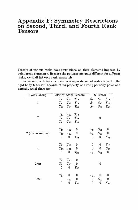
Tensors of various ranks have restrictions on their elements imposed by point group symmetry. Because the patterns are quite different for different ranks, we shall list each rank separately.
For second rank tensors there is a separate set of restrictions for the rigid body S tensor, because of its property of having partially polar and partially axial character.
Point Group Polar or Axial Tensors S Tensor T11 T12 T 13 511 512 513
1 Tn T22 Tn 521 522 523
T 13 T 23 T33 531 532 533
T11 T12 T 13
I T12 T22 T 23 0 T 13 T 23 T33
T11 T12 0 511 512 0 2 (z axis unique) T12 Tn 0 521 522 0
0 0 T33 0 0 533
T11 T12 0 0 0 513
m T12 T22 0 0 0 523
0 0 T33 531 532 0
T11 T12 0 21m T12 T22 0 0
0 0 T33
T11 0 0 511 0 0 222 0 T22 0 0 522 0
0 0 T33 0 0 533
182 Appendix F
Point Group
mm2
mmm
3,4,6
3, 4/m, 6, 6/m, 4/mmm, 3m,
6m2,6/mmm
32, 422, 622
3m, 4mm, 6mm
42m
23, 432 m3, 43m, m3m
Polar or Axial Tensors T11 0 0 o T22 0 o 0 T33
Tn 0 0 o T22 0 o 0 T33
Tn 0 0 o T22 0 o 0 T33
Tn 0 0 o Tn 0 o 0 T33
Tn 0 0 o T11 0 o 0 T33
Tu 0 0 o T11 0 o 0 T33
T11 0 0 o Tn 0 o 0 T33
T11 0 0 o Tu 0 o 0 T33
Tn 0 0 o Tu 0 o 0 Tu
S Tensor o S12 0
S21 0 0 o 0 0
o
S11 S12 0 -S12 S11 0
o 0 S33
S11 S12 0 S12 -S11 0 o 0 S33
o
S11 0 0 o S11 0 o 0 S33
o S12 0 -S12 0 0
o 0 0
S11 0 0 o -S11 0 o 0 0
o
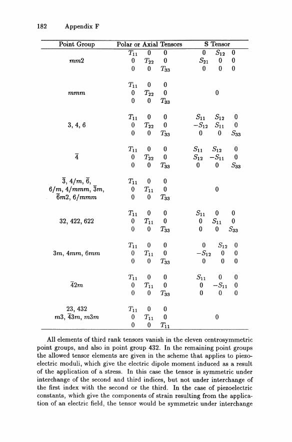
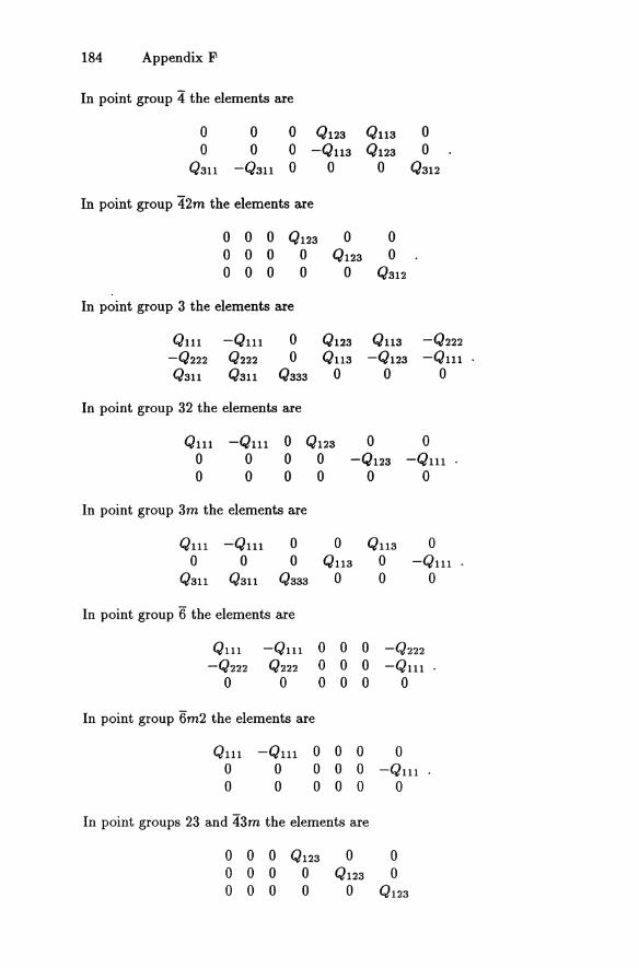
All elements of third rank tensors vanish in the eleven centrosymmetric point groups, and also in point group 432. In the remaining point groups the allowed tensor elements are given in the scheme that applies to piezoelectric moduli, which give the electric dipole moment induced as a result of the application of a stress. In this case the tensor is symmetric under interchange of the second and third indices, but not under interchange of the first index with the second or the third. In the case of piezoelectric constants, which give the components of strain resulting from the application of an electric field, the tensor would be symmetric under interchange
Symmetry Restrictions 183
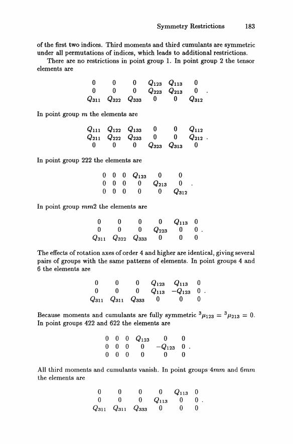
of the first two indices. Third moments and third cumulants are symmetric under all permutations of indices, which leads to additional restrictions.
There are no restrictions in point group 1. In point group 2 the tensor elements are
o 0 0 Q123 Q1l3 0 o 0 0 Q223 Q213 0
Q311 Q322 Q333 0 0 Q312
In point group m the elements are
In point group 222 the elements are
o 0 0 Q123
o 0 0 0 o 0 0 0
In point group mm2 the elements are
Q1l3 0 o 0 o 0
The effects of rotation axes of order 4 and higher are identical, giving several pairs of groups with the same patterns of elements. In point groups 4 and 6 the elements are
Q1l3 0 -Q123 0
o 0
Because moments and cumulants are fully symmetric 3Jl123 = 3 Jl213 = O. In point groups 422 and 622 the elements are
000 000 000
o 0 -Q123 0
o 0
All third moments and cumulants vanish. In point groups '4mm and 6mm the elements are
o Q113
o
Q113 0 o 0 o 0
184 Appendix F
In point group 4 the elements are
0 0 0 Q123 Q113 0 0 0 0 -QU3 Q123 0
Q3U -Q311 0 0 0 Q312
In point group 42m the elements are
0 0 0 Q123 0 0 0 0 0 0 Q123 0 0 0 0 0 0 Q312
In point group 3 the elements are
QU1 -QU1 0 Q123 QU3 -Q222
-Q222 Q222 0 QU3 -Q123 -QU1 Q3U Q3U Q333 0 0 0
In point group 32 the elements are
QU1 -Qu1 0 Q123 0 0 0 0 0 0 -Q123 -Qu1 0 0 0 0
In point group 3m the elements are
In point group 6 the elements are
0
QU3 o o
0
o -QU1
o
-Q111 0 0 0 -Q222
Q222 0 0 0 -Q111
o 0 0 0 0
In point group 6m2 the elements are
QU1 -QU1 0 0 0 0 0 0 0 0 0 -QU1 0 0 0 0 0 0
In point groups 23 and 43m the elements are
0 0 0 Q123 0 0 0 0 0 0 Q123 0 0 0 0 0 0 Q123
Symmetry Restrictions 185
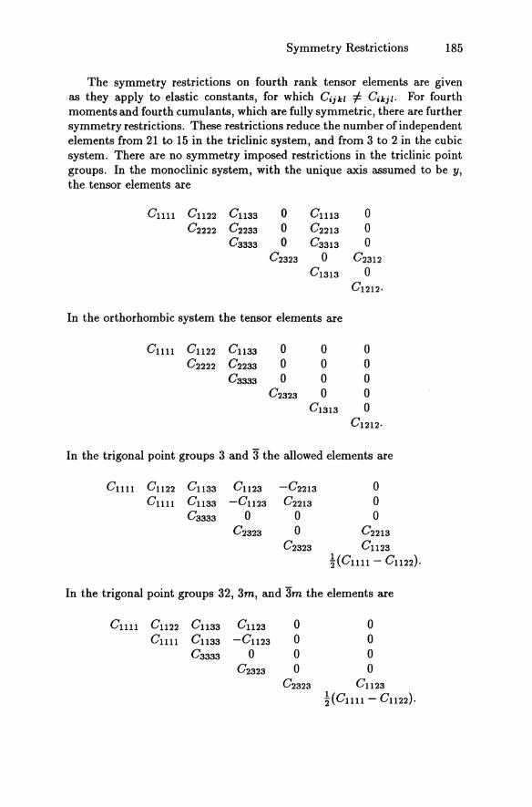
The symmetry restrictions on fourth rank tensor elements are given as they apply to elastic constants, for which Cijkl f:. Cikjl. For fourth moments and fourth cumulants, which are fully symmetric, there are further symmetry restrictions. These restrictions reduce the number of independent elements from 21 to 15 in the triclinic system, and from 3 to 2 in the cubic system. There are no symmetry imposed restrictions in the triclinic point groups. In the monoclinic system, with the unique axis assumed to be y, the tensor elements are
C uu C U22 C U33 0 C Ul3 0 C 2222 C 2233 0 C 22l3 0
C 3333 0 C 33l3 0 C2323 0 C 23l2
C 13I3 0
C l2I2 ·
In the orthorhombic system the tensor elements are
Cuu C U22 C U33 0 0 0 C 2222 C 2233 0 0 0
C3333 0 0 0 C2323 0 0
C l3l3 0 C 12I2 .
In the trigonal point groups 3 and 3 the allowed elements are
C UU C U22 C U33 C U23 -C22I3 0 C uu C U33 -CU23 C 22I3 0
C 3333 0 0 0 C 2323 0 C 2213
C 2323 CU23
HCuu - C U22).
In t.he trigonal point groups 32, 3m, and 3m the elements are
C UU C U22 C U33 C U23 0 0 C uu C ll33 -CU23 0 0
C 3333 0 0 0 C 2323 0 0
C 2323 C ll23
~(Cllll - C U22).
186 Appendix F
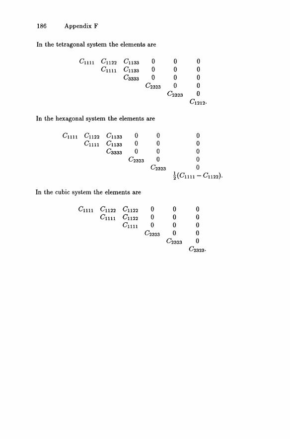
In the tetragonal system the elements are
C uu C U22 C ll33 0 0 0 C llll C 1l33 0 0 0
C 3333 0 0 0 C 2323 0 0
C 2323 0 C1212'
In the hexagonal system the elements are
CUll C 1l22 C 1l33 0 0 0 C uu C 1l33 0 0 0
C 3333 0 0 0 C 2323 0 0
C 2323 0 HCllll - C 1l22).
In the cubic system the elements are
CUll C U22 C 1l22 0 0 0 CUll C ll22 0 0 0
CUll 0 0 0 C 2323 0 0
C 2323 0
C 2323 ·
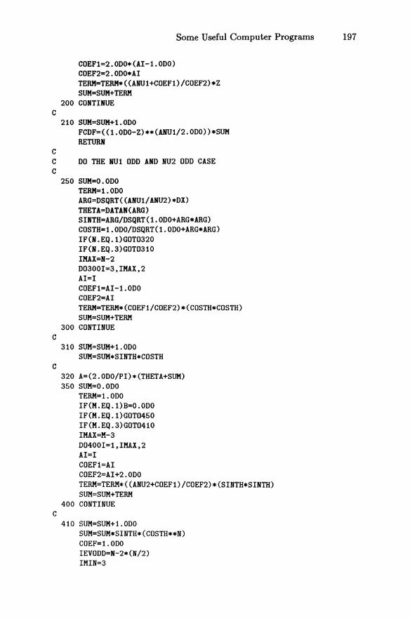
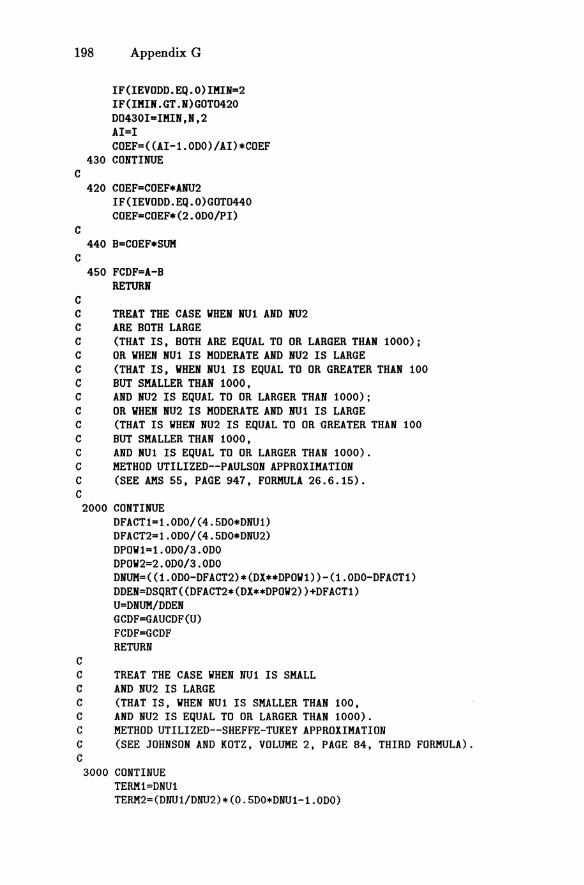
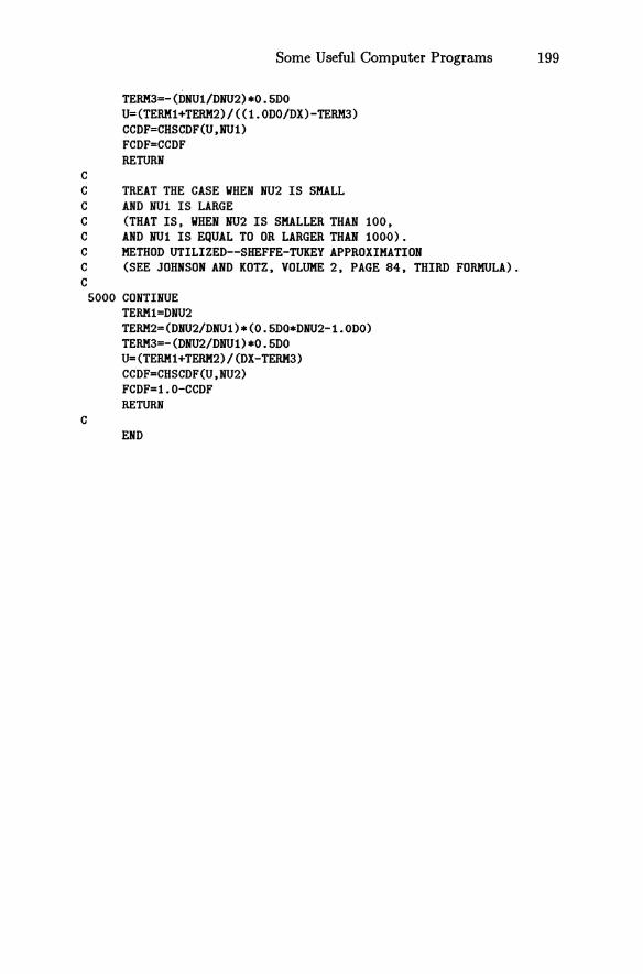
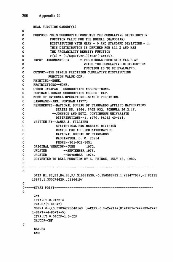
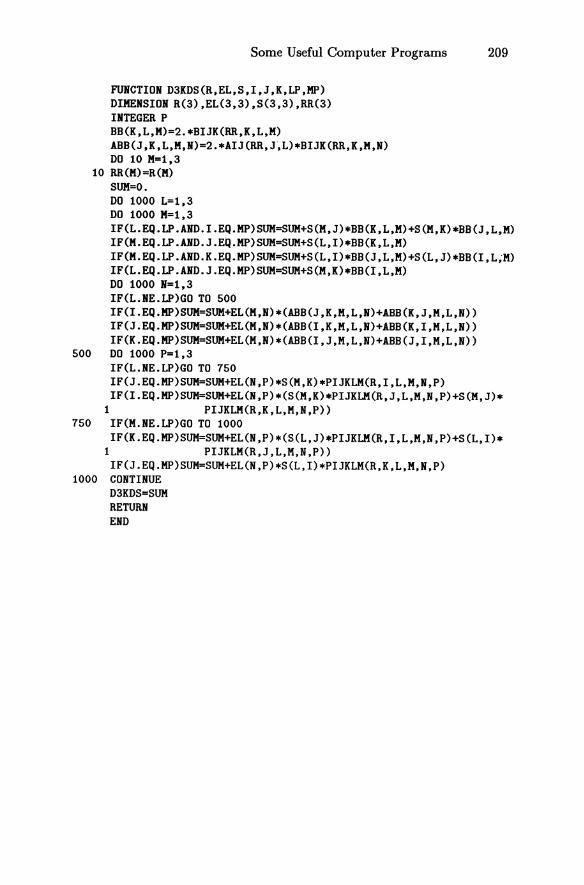
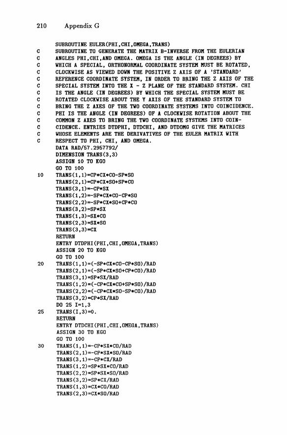
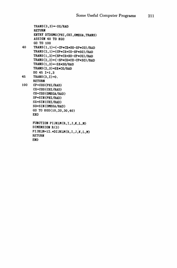
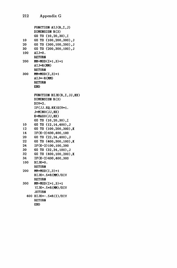
Appendix G: Some Useful Computer Programs
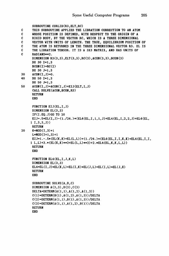
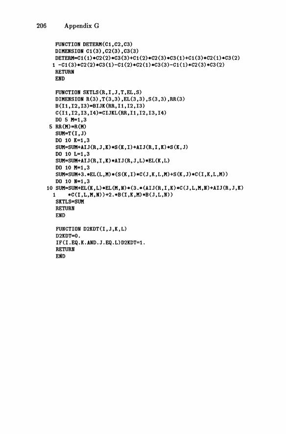
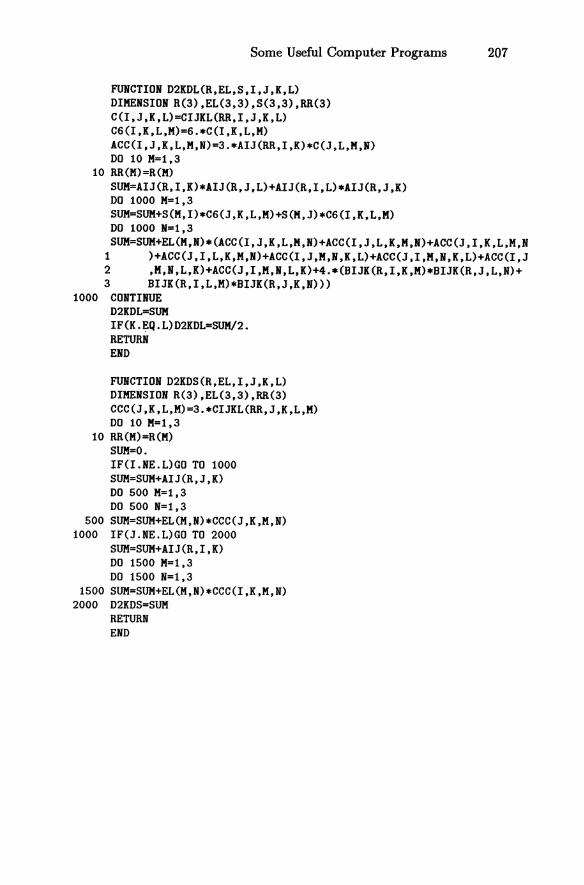
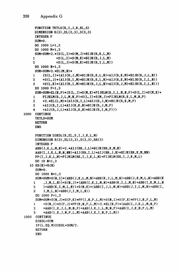
On the following pages we reproduce FORTRAN source code for a number of useful mathematical operations, including the important statistical distribution functions. Also included are code for the libration correction - the function ElJ is the matrix (1 + M) discussed in chapter 9 - and for shape and rigid-body-motion constraints. I am indebted to James J. Filliben for permission to use the statistical functions.
188 Appendix G
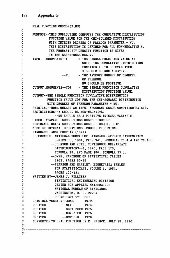
REAL FUNCTION CHSCDF(X,HU) C C PURPOSE--THIS SUBROUTINE COMPUTES THE CUMULATIVE DISTRIBUTION C FUNCTION VALUE FOR THE CHI-SQUARED DISTRIBUTION C WITH INTEGER DEGREES OF FREEDOM PARAMETER = HU. C THIS DISTRIBUTION IS DEFINED FOR ALL NON-NEGATIVE X. C THE PROBABILITY DENSITY FUNCTION IS GIVEN C IN THE REFERENCES BELOW. C INPUT ARGUMENTS--X = THE SINGLE PRECISION VALUE AT C WHICH THE CUMULATIVE DISTRIBUTION C FUNCTION IS TO BE EVALUATED. C X SHOULD BE NON-NEGATIVE. C C C C
--NO
OUTPUT ARGUMENTS--CDF
= THE INTEGER NUMBER OF DEGREES OF FREEDOM. HU SHOULD BE POSITIVE.
= THE SINGLE PRECISION CUMULATIVE C DISTRIBUTION FUNCTION VALUE. C OUTPUT--THE SINGLE PRECISION CUMULATIVE DISTRIBUTION C FUNCTION VALUE CDF FOR THE CHI-SQUARED DISTRIBUTION C WITH DEGREES OF FREEDOM PARAMETER = HU. C PRINTING--NONE UNLESS AN INPUT ARGUMENT ERROR CONDITION EXISTS. C RESTRICTIONS--X SHOULD BE NON-NEGATIVE. C --NU SHOULD BE A POSITIVE INTEGER VARIABLE. C OTHER DATAPAC SUBROUTINES NEEDED--NORCDF. C FORTRAN LIBRARY SUBROUTINES NEEDED--DSQRT, DEXP. C MODE OF INTERNAL OPERATIONS--DOUBLE PRECISION. C LANGUAGE--ANSI FORTRAN (1977) C REFERENCES--NATIONAL BUREAU OF STANDARDS APPLIED MATHEMATICS C SERIES 55, 1964, PAGE 941, FORMULAE 26.4.4 AND 26.4.5. C --JOHNSON AND KOTZ, CONTINUOUS UNIVARIATE C DISTRIBUTIONS--1, 1970, PAGE 176, C FORMULA 28, AND PAGE 180, FORMULA 33.1. C --OWEN, HANDBOOK OF STATISTICAL TABLES, C 1962, PAGES 50-55. C --PEARSON AND HARTLEY, BIOMETRIKA TABLES C FOR STATISTICIANS, VOLUME 1, 1954, C PAGES 122-131. C WRITTEN BY--JAMES J. FILLIBEN C STATISTICAL ENGINEERING DIVISION C CENTER FOR APPLIED MATHEMATICS C NATIONAL BUREAU OF STANDARDS C WASHINGTON, D. C. 20234 C PHONE--301-921-3651 C ORIGINAL VERSION--JUNE 1972. C UPDATED --MAY 1974. C UPDATED --SEPTEMBER 1975. C C
UPDATED UPDATED
--NOVEMBER 1975. --OCTOBER 1976.
C CONVERTED TO REAL FUNCTION BY E. PRINCE, JULY 18, 1980. C
C---------------------------------------------------------------------C
C
Some Useful Computer Programs 189
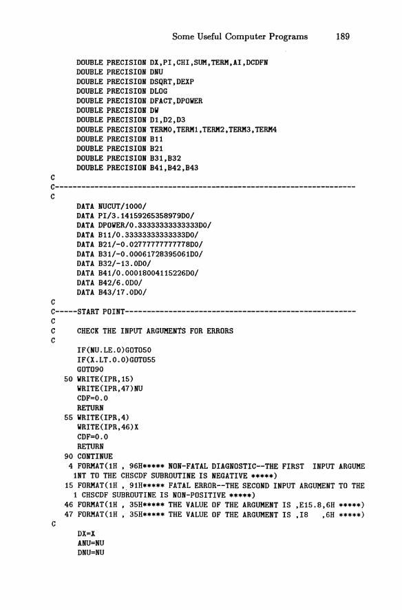
DOUBLE PRECISION DX,PI,CHI,SUM,TERM,AI,DCDFN DOUBLE PRECISION DNU DOUBLE PRECISION DSQRT,DEXP DOUBLE PRECISION DLOG DOUBLE PRECISION DFACT,DPOWER DOUBLE PRECISION DW DOUBLE PRECISION D1,D2,D3 DOUBLE PRECISION TERMO, TERM1, TERM2, TERM3, TERM4 DOUBLE PRECISION Bll DOUBLE PRECISION B21 DOUBLE PRECISION B31,B32 DOUBLE PRECISION B41,B42,B43
C---------------------------------------------------------------------C
C
DATA NUCUT/1000/ DATA PI/3.14159265358979DO/ DATA DPOWER/0.33333333333333DO/ DATA B11/0.33333333333333DO/ DATA B21/-0.02777777777778DO/ DATA B31/-0.00061728395061DO/ DATA B32/-13.0DO/ DATA B41/0.00018004115226DO/ DATA B42/6.0DO/ DATA B43/17.0DO/
C-----START POINT-----------------------------------------------------C C CHECK THE INPUT ARGUMENTS FOR ERRORS C
C
IF(NU.LE.0)GOT050 IF(X.LT.0.O)GOT055 GOT090
50 WRITE(IPR,15) WRITE(IPR,47)NU CDF=O.O RETURN
55 WRITE(IPR,4) WRITE(IPR,46)X CDF=O.O RETURN
90 CONTINUE 4 FORMAT(lH , 96H***** NON-FATAL DIAGNOSTIC--THE FIRST INPUT ARGUME
lNT TO THE CHSCDF SUBROUTINE IS NEGATIVE *****) 15 FORMAT(lH ,.91H***** FATAL ERROR--THE SECOND INPUT ARGUMENT TO THE
1 CHSCDF SUBROUTINE IS NON-POSITIVE *****) 46 FORMAT(lH , 35H***** THE VALUE OF THE ARGUMENT IS ,E15.8,6H *****) 47 FORMAT(lH , 35H***** THE VALUE OF THE ARGUMENT IS ,18 ,6H *****)
DX=X ANU=NU DNU=NU
190 Appendix G
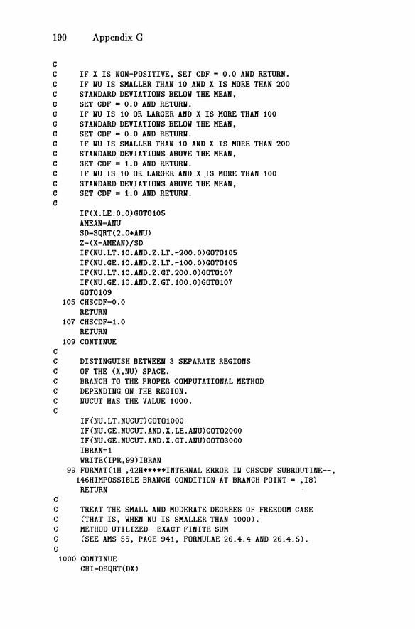
C C IF X IS NON-POSITIVE, SET CDF = 0.0 AND RETURN. C IF NU IS SMALLER THAN 10 AND X IS MORE THAN 200 C STANDARD DEVIATIONS BELOW THE MEAN, C SET CDF = 0.0 AND RETURN. C IF NU IS 10 OR LARGER AND X IS MORE THAN 100 C STANDARD DEVIATIONS BELOW THE MEAN, C SET CDF = 0.0 AND RETURN. C IF NU IS SMALLER THAN 10 AND X IS MORE THAN 200 C STANDARD DEVIATIONS ABOVE THE MEAN, C SET CDF = 1.0 AND RETURN. C IF NU IS 10 OR LARGER AND X JS MORE THAN 100 C STANDARD DEVIATIONS ABOVE THE MEAN, C SET CDF = 1.0 AND RETURN. C
C
IF(X.LE.0.0)GOT0105 AMEAN=ANU SD=SQRT(2.0*ANO) Z=(X-AMEAN)/SD IF(NU.LT.l0.AND.Z.LT.-200.0)GOTol05 IF(NU.GE.l0.AND.Z.LT.-l00.0)GOT0105 IF(NU.LT.l0.AND.Z.GT.200.0)GoT0107 IF(NU.GE.l0.AND.Z.GT.l00.0)GOTol07 GoT0109
105 CHSCDF=O.O RETURN
107 CHSCDF=1.0 RETURN
109 CONTINUE
C DISTINGUISH BETWEEN 3 SEPARATE REGIONS C OF THE (X,NU) SPACE. C BRANCH TO THE PROPER COMPUTATIONAL METHOD C DEPENDING ON THE REGION. C NUCUT HAS THE VALUE 1000. C
IF(NU.LT.NUCUT)GOTol000 IF(NU.GE.NUCUT.AND.X.LE.ANU)GoT02000 IF(NU.GE.NUCUT.AND.X.GT.ANU)GoT03000 IBRAN=l WRITE(IPR,99)IBRAN
99 FoRMAT(lH ,42H*****INTERNAL ERROR IN CHSCDF SUBRoUTINE--, 146HIMPOSSIBLE BRANCH CONDITION AT BRANCH POINT = ,18)
RETURN C C TREAT THE SMALL AND MODERATE DEGREES OF FREEDOM CASE C (THAT IS, WHEN NO IS SMALLER THAN 1000). C METHOD UTILIZED--EXACT FINITE SUM C (SEE AMS 55, PAGE 941, FORMULAE 26.4.4 AND 26.4.5). C
1000 CONTINUE CHI=DSQRT(DX)
C
C
C
C
C
Some Useful Computer Programs 191
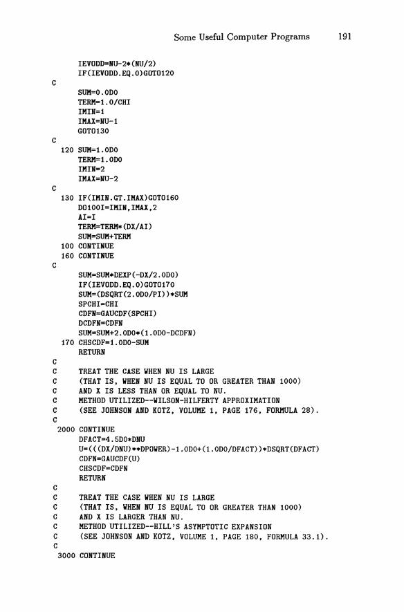
IEVODD=NU-2*(NU/2) IF(IEVODD.EQ.0)GOT0120
SUM=O.ODO TERM=1.0/CHI IMIN=l lMAX=NU-l GOT0130
120 SUM=1.0DO TERM=1.0DO IMIN=2 lMAX=NU-2
130 IF(IMIN.GT.lMAX)GOT0160 D0100I=IMIN,IMAX,2 AI=I TERM=TERM*(DX/AI) StJlot=SUM+TERM
100 CONTINUE 160 CONTINUE
SUM=SUM*DEXP(-DX/2.0DO) IF(IEVODD.EQ.0)GOT0170 SUM=(DSQRT(2.0DO/PI»*SUM SPCHI=CHI CDFN=GAUCDF(SPCHI) DCDFN=CDFN SUM=SUM+2.0DO*(1.0DO-DCDFN)
170 CHSCDF=1.0DO-SUM RETURN
C TREAT THE CASE WHEN NU IS LARGE C (THAT IS, WHEN NU IS EQUAL TO OR GREATER THAN 1000) C AND X IS LESS THAN OR EQUAL TO NU. C METHOD UTILIZED--WILSON-HILFERTY APPROXIMATION C (SEE JOHNSON AND KOTZ, VOLUME 1, PAGE 176, FORMULA 28). C
C
2000 CONTINUE DFACT=4.5DO*DHU U=«(DX/DHU)**DPOWER)-1.0DO+(1.0DO/DFACT»*DSQRT(DFACT) CDFN=GAUCDF(U) CHSCDF=CDFN RETURN
C TREAT THE CASE WHEN NU IS LARGE C (THAT IS, WHEN NU IS EQUAL TO OR GREATER THAN 1000) C AND X IS LARGER THAN HU. C METHOD UTILIZED--HILL'S ASYMPTOTIC EXPANSION C (SEE JOHNSON AND KOTZ, VOLUME 1, PAGE 180, FORMULA 33.1). C 3000 CONTINUE

192 Appendix G
C
DW=DSQRT(DX-DNU-DNU*DLOG(DX/DNU)) DANU=DSQRT(2.0DO/DNU) Dl=DW D2=DW**2 D3=DW**3 TERMO=DW TERM1=Bll*DANU TERM2=B21*Dl*(DANU**2) TERM3=B31* (D2+B32) * (DANU**3) TERM4=B41*(B42*D3+B43*Dl)*(DANU**4) U=TERMO+TERM1+TERM2+TERH3+TERM4 CDFN=GAUCDF(U) CHSCDF=CDFN RETURN
END
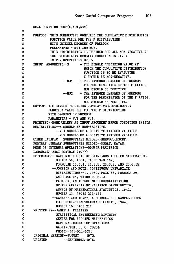
Some Useful Computer Programs 193
REAL FUNCTION FCDF(X,NU1,NU2) C C PURPOSE--THIS SUBROUTINE COMPUTES THE CUMULATIVE DISTRIBUTION C FUNCTION VALUE FOR THE F DISTRIBUTION C WITH INTEGER DEGREES OF FREEDOM C PARAMETERS = NUl AND NU2. C THIS DISTRIBUTION IS DEFINED FOR ALL NON-NEGATIVE X. C THE PROBABILITY DENSITY FUNCTION IS GIVEN C IN THE REFERENCES BELOW. C INPUT ARGUMENTS--X = THE SINGLE PRECISION VALUE AT C WHICH THE CUMULATIVE DISTRIBUTION C FUNCTION IS TO BE EVALUATED. C X SHOULD BE NON-NEGATIVE. C C C C C
--NUl
--NU2
= THE INTEGER DEGREES OF FREEDOM FOR THE NUMERATOR OF THE F RATIO. NUl SHOULD BE POSITIVE.
= THE INTEGER DEGREES OF FREEDOM FOR THE DENOMINATOR OF THE F RATIO.
C NU2 SHOULD BE POSITIVE. C OUTPUT--THE SINGLE PRECISION CUMULATIVE DISTRIBUTION C FUNCTION VALUE CDF FOR THE F DISTRIBUTION C WITH DEGREES OF FREEDOM C PARAMETERS = NUl AND NU2. C PRINTING--NONE UNLESS AN INPUT ARGUMENT ERROR CONDITION EXISTS. C RESTRICTIONS--X SHOULD BE NON-NEGATIVE. C --NUl SHOULD BE A POSITIVE INTEGER VARIABLE. C --NU2 SHOULD BE A POSITIVE INTEGER VARIABLE. C OTHER DATAPAC SUBROUTINES NEEDED--NORCDF,CHSCDF. C FORTRAN LIBRARY SUBROUTINES NEEDED--DSQRT, DATAN. C MODE OF INTERNAL OPERATIONS--DOUBLE PRECISION. C LANGUAGE--ANSI FORTRAN (1977) C REFERENCES--NATIONAL BUREAU OF STANDARDS APPLIED MATHEMATICS C SERIES 55, 1964, PAGES 946-947, C FORMULAE 26.6.4,26.6.5, 26.6.8, AND 26.6.15. C --JOHNSON AND KOTZ, CONTINUOUS UNIVARIATE C DISTRIBUTIONS--2, 1970, PAGE 83, FORMULA 20, C AND PAGE 84, THIRD FORMULA. C --PAULSON, AN APPROXIMATE NORHAILIZATION C OF THE ANALYSIS OF VARIANCE DISTRIBUTION, C ANNALS OF MATHEMATICAL STATISTICS, 1942, C NUMBER 13, PAGES 233-135. C --SCHEFFE AND TUKEY, A FORMULA FOR SAMPLE SIZES C FOR POPULATION TOLERANCE LIMITS, 1944, C NUMBER 15, PAGE 217. C WRITTEN BY--JAMES J. FILLIBEN C STATISTICAL ENGINEERING DIVISION C CENTER FOR APPLIED MATHEMATICS C NATIONAL BUREAU OF STANDARDS C WASHINGTON, D. C. 20234 C PHONE--301-921-3651 C ORIGINAL VERSION--AUGUST 1972. C UPDATED --SEPTEMBER 1975.
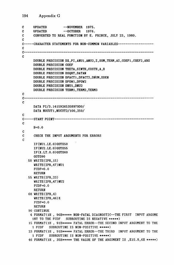
194 Appendix G
C C
UPDATED UPDATED
--NOVEMBER 1975. --OCTOBER 1976.
C CONVERTED TO REAL FUNCTION BY E. PRINCE, JULY 23, 1980. C C-----CHARACTER STATEMENTS FOR NON-COMMON VARIABLES------------------C
C---------------------------------------------------------------------C
C
DOUBLE PRECISION DX,PI,ANU1,ANU2,Z,SUM,TERM,AI,COEF1,COEF2,ARG DOUBLE PRECISION COEF DOUBLE PRECISION THETA,SINTH,COSTH,A,B DOUBLE PRECISION DSQRT,DATAN DOUBLE PRECISION DFACT1,DFACT2,DNUM,DDEN DOUBLE PRECISION DPOW1,DPOW2 DOUBLE PRECISION DNU1,DNU2 DOUBLE PRECISION TERM1,TERM2,TERM3
C---------------------------------------------------------------------C
C
DATA PI/3.14159265358979DO/ DATA NUCUT1,NUCUT2/100,250/
C-----START POINT-----------------------------------------------------C
B=O.O C C CHECK THE INPUT ARGUMENTS FOR ERRORS C
IF(NU1.LE.0)GOT050 IF(NU2.LE.0)GOT055 IF(X.LT.0.0)GOT060 GOT090
50 WRITE(IPR,15) WRITE(IPR,47)NUl FCDF=O.O RETURN
55 WRITE(IPR,23) WRITE(IPR,47)NU2 FCDF=O.O RETURN
60 WRITE(IPR,4) WRITE(IPR,46)X FCDF=O.O RETURN
90 CONTINUE 4 FORMAT(lH , 96H***** NON-FATAL DIAGNOSTIC--THE FIRST INPUT ARGUME
lNT TO THE FCDF SUBROUTINE IS NEGATIVE *****) 15 FORMAT(lH , 91H***** FATAL ERROR--THE SECOND INPUT ARGUMENT TO THE
1 FCDF SUBROUTINE IS NON-POSITIVE *****) 23 FORMAT(lH , 91H***** FATAL ERROR--THE THIRD INPUT ARGUMENT TO THE
1 FCDF SUBROUTINE IS NON-POSITIVE *****) 46 FORMAT(lH , 35H***** THE VALUE OF THE ARGUMENT IS ,E15.8,6H *****)
C
C
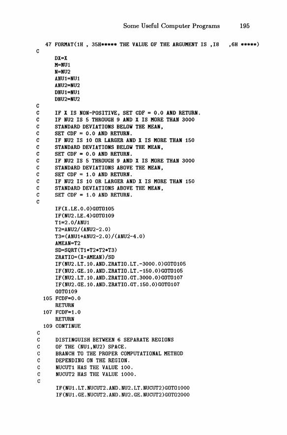
Some Useful Computer Programs 195
47 FORMAT(lH , 35H***** THE VALUE OF THE ARGUMENT IS ,18 ,6H *****)
DX=X M=NUl N=NU2 ANU1=NUl ANU2=NU2 DNUl =NU 1 DNU2=NU2
C IF X IS NON-POSITIVE, SET CDF = 0.0 AND RETURN. C IF NU2 IS 5 THROUGH 9 AND X IS MORE THAN 3000 C STANDARD DEVIATIONS BELOW THE MEAN, C SET CDF = 0.0 AND RETURN. C IF NU2 IS 10 OR LARGER AND X IS MORE THAN 150 C STANDARD DEVIATIONS BELOW THE MEAN, C SET CDF = 0.0 AND RETURN. C IF NU2 IS 5 THROUGH 9 AND X IS MORE THAN 3000 C STANDARD DEVIATIONS ABOVE THE MEAN, C SET CDF = 1.0 AND RETURN. C IF NU2 IS 10 OR LARGER AND X IS MORE THAN 150 C STANDARD DEVIATIONS ABOVE THE MEAN, C SET CDF = 1.0 AND RETURN. C
C
IF(X.LE.0.0)GOT0105 IF(NU2.LE.4)GOT0109 Tl=2.0/ANUl T2=ANU2/(ANU2-2.0) T3=(ANU1+ANU2-2.0)/(ANU2-4.0) AMEAN=T2 SD=SQRT(Tl*T2*T2*T3) ZRATIO=(X-AMEAN)/SD IF(NU2.LT.l0.AND.ZRATIO.LT.-3000.0)GOT0105 IF(NU2.GE.l0.AND.ZRATIO.LT.-150.0)GOT0105 IF(NU2.LT.l0.AND.ZRATIO.GT.3000.0)GOT0107 IF(NU2.GE.l0.AND.ZRATIO.GT.150.0)GOT0107 GOT0109
105 FCDF=O.O RETURN
107 FCDF=1.0 RETURN
109 CONTINUE
C DISTINGUISH BETWEEN 6 SEPARATE REGIONS C OF THE (NU1,NU2) SPACE. C BRANCH TO THE PROPER COMPUTATIONAL METHOD C DEPENDING ON THE REGION. C NUCUTl HAS THE VALUE 100. C NUCUT2 HAS THE VALUE 1000. C
IF(NU1.LT.NUCUT2.AND.NU2.LT.NUCUT2)GOT01000 IF(NU1.GE.NUCUT2.AND.NU2.GE.NUCUT2)GOT02000
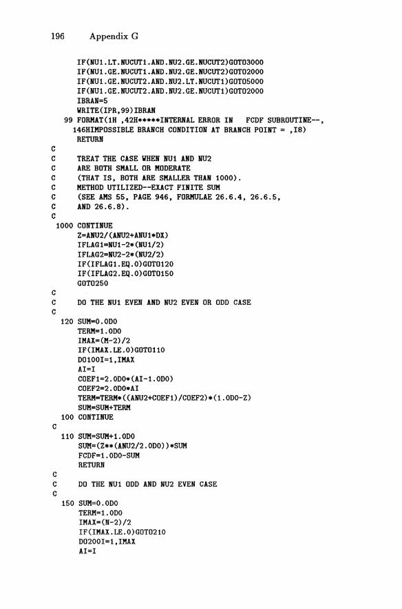
196 Appendix G
C
IF(NU1.LT.NUCUT1.AND.NU2.GE.NUCUT2)GOT03000 IF(NU1.GE.NUCUT1.AND.NU2.GE.NUCUT2)GOT02000 IF(NU1.GE.NUCUT2.AND.NU2.LT.NUCUT1)GOT05000 IF(NU1.GE.NUCUT2.AND.NU2.GE.NUCUT1)GOT02000 IBRAN=5 WRITE(IPR,99)IBRAN
99 FORMAT(lH ,42H*****INTERNAL ERROR IN FCDF SUBROUTINE--, 146HIMPOSSIBLE BRANCH CONDITION AT BRANCH POINT = ,18)
RETURN
C TREAT THE CASE WHEN NUl AND NU2 C ARE BOTH SMALL OR MODERATE C (THAT IS, BOTH ARE SMALLER THAN 1000). C METHOD UTILIZED--EXACT FINITE SUM C (SEE AMS 55, PAGE 946, FORMULAE 26.6.4, 26.6.5, C AND 26.6.8). C
C
1000 CONTINUE Z=ANU2/(ANU2+ANU1*DX) IFLAG1=NUl-2*(NU1/2) IFLAG2=NU2-2*(NU2/2) IF(IFLAG1.EQ.0)GOT0120 IF(IFLAG2.EQ.0)GOT0150 GOT0250
C DO THE NUl EVEN AND NU2 EVEN OR ODD CASE C
C
C
120 SUM=O.ODO TERM=1.0DO IMAX=(M-2)/2 IF(IMAX.LE.0)GOTOll0 D0100I=l,IMAX AI=I COEF1=2.0DO*(AI-1.0DO) COEF2=2.0DOdI TERM=TERM*«ANU2+COEF1)/COEF2)*(1.0DO-Z) SUM=SUM+TERM
100 CONTINUE
110 SUM=SUM+l.0DO SUM=(Z**(ANU2/2.0DO»*SUM FCDF=1.0DO-SUM RETURN
C DO THE NUl ODD AND NU2 EVEN CASE C
150 SUM=O.ODO TERM=1.0DO IMAX=(N-2)/2 IF(IMAX.LE.O)GDT0210 D0200I=l,IMAX AI=I
COEF1=2.0DO*(AI-l.0DO) COEF2=2.0DO*AI
Some Useful Computer Programs 197
TERH=TERH* «ANU1+COEF1)/COEF2) *Z SUM=SUM+TERH
200 CONTINUE C
C
210 SUM=SUM+l.0DO FCDF=«1.0DO-Z)**(ANU1/2.0DO»*SUM RETURN
C DO THE NUl ODD AND NU2 ODD CASE C
C
C
250 SUM=O.ODO TERH=1.0DO ARG=DSQRT«ANU1/ANU2)*DX) THETA=DATAN(ARG) SINTH=ARG/DSQRT(1.0DO+ARG*ARG) COSTH=1.0DO/DSQRT(1.0DO+ARG*ARG) IF(N.EQ.l)GOT0320 IF(N.EQ.3)GOT0310 IMAX=N-2 D0300I=3,IMAX,2 AI=I COEF1=AI-l.0DO COEF2=AI TERH=TERH*(COEF1/COEF2)*(COSTH*COSTH) SUM=SUM+TERM
300 CONTINUE
310 SUM=SUM+l.0DO SUM=SUM*SINTH*COSTH
320 A=(2.0DO/PI)*(THETA+SUM) 350 SUM=O.ODO
TERM=1.0DO IF(M.EQ.l)B=O.ODO IF(M.EQ.l)GOT0450 IF(M.EQ.3)GOT0410 IMAX=M-3 D0400I=l,IMAX,2 AI=I COEF1=AI COEF2=AI+2.0DO TERH=TERM*«ANU2+COEF1)/COEF2)* (SINTH*SINTH) SUM=SUM+TERM
400 CONTINUE C
410 SUM=SUM+1.0DO SUM=SUM*SINTH*(COSTH**N) COEF=1.0DO IEVODD=N-2*(N/2) IMIN=3
198 Appendix G
C
C
C
C
IF(IEVODD.EQ.0)IMIN=2 IF(IMIN.GT.N)GOT0420 D0430I=IMIN,N,2 AI=I COEF=«AI-l.0DO)/AI)*COEF
430 CONTINUE
420 COEF=COEF*ANU2 IF(IEVODD.EQ.0)GOT0440 COEF=COEF*(2.0DO/PI)
450 FCDF=A-B RETURN
C TREAT THE CASE WHEN NUl AND NU2 C ARE BOTH LARGE C (THAT IS, BOTH ARE EQUAL TO OR LARGER THAN 1000); C OR WHEN NUl IS MODERATE AND NU2 IS LARGE C (THAT IS, WHEN NUl IS EQUAL TO OR GREATER THAN 100 C BUT SMALLER THAN 1000, C AND NU2 IS EQUAL TO OR LARGER THAN 1000); C OR WHEN NU2 IS MODERATE AND NUl IS LARGE C (THAT IS WHEN NU2 IS EQUAL TO OR GREATER THAN 100 C BUT SMALLER THAN 1000, C AND NUl IS EQUAL TO OR LARGER THAN 1000). C METHOD UTILIZED--PAULSON APPROXIMATION C (SEE AMS 55, PAGE 947, FORMULA 26.6.15). C 2000 CONTINUE
C
DFACT1=1.0DO/(4.5DO*DNU1) DFACT2=1.0DO/(4.5DO*DNU2) DPOW1=1.ODO/3.0DO DPOW2=2.0DO/3.0DO DNUM=«1.ODO-DFACT2)*(DX**DPOW1»-(1.ODO-DFACT1) DDEN=DSQRT«DFACT2*(DX**DPOW2»+DFACT1) U=DNUM/DDEN GCDF=GAUCDF(U) FCDF=GCDF RETURN
C TREAT THE CASE WHEN NUl IS SMALL C AND NU2 IS LARGE C (THAT IS, WHEN NUl IS SMALLER THAN 100, C AND NU2 IS EQUAL TO OR LARGER THAN 1000). C METHOD UTILIZED--SHEFFE-TUKEY APPROXIMATION C (SEE JOHNSON AND KOTZ, VOLUME 2, PAGE 84, THIRD FORMULA). C
3000 CONTINUE TERM1=DNUl TERM2=(DNU1/DNU2)*(0.5DO*DNU1-l.ODO)
C
Some Useful Computer Programs 199
TERM3=-(DNU1/DNU2)*0.5DO U=(TERM1+TERM2)/«1.0DO/DX)-TERM3) CCDF=CHSCDF(U.NU1) FCDF=CCDF RETURN
C TREAT THE CASE WHEN NU2 IS SMALL C AND NUl IS LARGE C (THAT IS. WHEN NU2 IS SMALLER THAN 100. C AND NUl IS EQUAL TO OR LARGER THAN 1000). C METHOD UTILIZED--SHEFFE-TUKEY APPROXIMATION C (SEE JOHNSON AND KOTZ. VOLUME 2. PAGE 84. THIRD FORMULA). C
C
5000 CONTINUE TERM 1 =DNU2 TERM2=(DNU2/DNU1)*(0.5DO*DNU2-1.0DO) TERM3=-(DNU2/DNU1)*O.5DO U=(TERM1+TERM2)/(DX-TERM3) CCDF=CHSCDF(U.NU2) FCDF=1.0-CCDF RETURN
END
200 Appendix G
REAL FUNCTION GAUCDF(X) c C PURPOSE--THIS SUBROUTINE COMPUTES THE CUMULATIVE DISTRIBUTION C FUNCTION VALUE FOR THE NORMAL (GAUSSIAN) C DISTRIBUTION WITH MEAN = 0 AND STANDARD DEVIATION = 1. C THIS DISTRIBUTION IS DEFINED FOR ALL X AND HAS C THE PROBABILITY DENSITY FUNCTION C F(X) = (1/SQRT(2*PI»*EXP(-X*X/2). C INPUT ARGUMENTS--X = THE SINGLE PRECISION VALUE AT C WHICH THE CUMULATIVE DISTRIBUTION C FUNCTION IS TO BE EVALUATED. C OUTPUT--THE SINGLE PRECISION CUMULATIVE DISTRIBUTION C FUNCTION VALUE CDF. C PRINTING--NONE. C RESTRICTIONS--NONE. C OTHER DATAPAC SUBROUTINES NEEDED--NONE. C FORTRAN LIBRARY SUBROUTINES NEEDED--EXP. C MODE OF INTERNAL OPERATIONS--SINGLE PRECISION. C LANGUAGE--ANSI FORTRAN (1977) C REFERENCES--NATIONAL BUREAU OF STANDARDS APPLIED MATHEMATICS C SERIES 55, 1964, PAGE 932, FORMULA 26.2.17. C --JOHNSON AND KOTZ, CONTINUOUS UNIVARIATE C DISTRIBUTIONS--l, 1970, PAGES 40-111. C WRITTEN BY--JAMES J. FILLIBEN C STATISTICAL ENGINEERING DIVISION C CENTER FOR APPLIED MATHEMATICS C NATIONAL BUREAU OF STANDARDS C WASHINGTON, D. C. 20234 C PHONE--301-921-3651 C ORIGINAL VERSION--JUNE 1972. C UPDATED --SEPTEMBE~ 1975. C UPDATED --NOVEMBER 1975. C CONVERTED TO REAL FUNCTION BY E. PRINCE, JULY 18, 1980. C
C---------------------------------------------------------------------C
C
DATA Bl,B2,B3,B4,B5,P/.319381530,-0.356563782,l.781477937,-1.82125 15978,1.330274429,.2316419/
C-----START POINT-----------------------------------------------------C
C
Z=X IF(X.LT.O.O)Z=-Z T=l. 0/ (1. O+P*Z) CDF=1.0-«0.39894228040143 )*EXP(-0.5*Z*Z»*(Bl*T+B2*T**2+B3*T**3
1+B4*T**4+B5*T**5) IF(X.LT.0.0)CDF=1.0-CDF GAUCDF=CDF
RETURN END
Some Useful Computer Programs 201
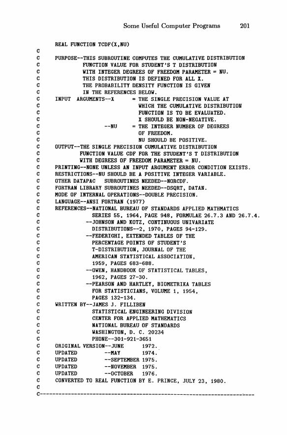
REAL FUNCTION TCDF(X,NU) C C PURPOSE--THIS SUBROUTINE COMPUTES THE CUMULATIVE DISTRIBUTION C FUNCTION VALUE FOR STUDENT'S T DISTRIBUTION C WITH INTEGER DEGREES OF FREEDOM PARAMETER = NU. C THIS DISTRIBUTION IS DEFINED FOR ALL X. C THE PROBABILITY DENSITY FUNCTION IS GIVEN C IN THE REFERENCES BELOW. C C C C C C
INPUT ARGUMENTS--X
--NU
= THE SINGLE PRECISION VALUE AT WHICH THE CUMULATIVE DISTRIBUTION FUNCTION IS TO BE EVALUATED. X SHOULD BE NON-NEGATIVE.
= THE INTEGER NUMBER OF DEGREES OF FREEDOM.
C NU SHOULD BE POSITIVE. C OUTPUT--THE SINGLE PRECISION CUMULATIVE DISTRIBUTION C FUNCTION VALUE CDF FOR THE STUDENT'S T DISTRIBUTION C WITH DEGREES OF FREEDOM PARAMETER = NU. C PRINTING--NONE UNLESS AN INPUT ARGUMENT ERROR CONDITION EXISTS. C RESTRICTIONS--NU SHOULD BE A POSITIVE INTEGER VARIABLE. C OTHER DATAPAC SUBROUTINES NEEDED--NORCDF. C C C C C C C C C C C C C C C C C C C C C C C C C C C C
FORTRAN LIBRARY SUBROUTINES NEEDED--DSQRT, DATAN. MODE OF INTERNAL OPERATIONS--DOUBLE PRECISION. LANGUAGE--ANSI FORTRAN (1977) REFERENCES--NATIONAL BUREAU OF STANDARDS APPLIED MATHKATICS
SERIES 55, 1964, PAGE 948, FORMULAE 26.7.3 AND 26.7.4. --JOHNSON AND KOTZ, CONTINUOUS UNIVARIATE
DISTRIBUTIONS--2, 1970, PAGES 94-129. --FEDERIGHI, EXTENDED TABLES OF THE
PERCENTAGE POINTS OF STUDENT'S T-DISTRIBUTION, JOURNAL OF THE AMERICAN STATISTICAL ASSOCIATION, 1959, PAGES 683-688.
--OWEN, HANDBOOK OF STATISTICAL TABLES, 1962, PAGES 27-30.
--PEARSON AND HARTLEY, BIOMETRIKA TABLES FOR STATISTICIANS, VOLUME 1, 1954, PAGES 132-134.
WRITTEN BY--JAMES J. FILLIBEN STATISTICAL ENGINEERING DIVISION CENTER FOR APPLIED MATHEMATICS NATIONAL BUREAU OF STANDARDS WASHINGTON, D. C. 20234 PHONE--301-921-3651
ORIGINAL VERSION--JUNE 1972. UPDATED --MAY 1974. UPDATED UPDATED UPDATED
--SEPTEMBER 1975. --NOVEMBER 1975. --OCTOBER 1976.
C CONVERTED TO REAL FUNCTION BY E. PRINCE, JULY 23, 1980. C
C-----------------------------------------------------------------~---
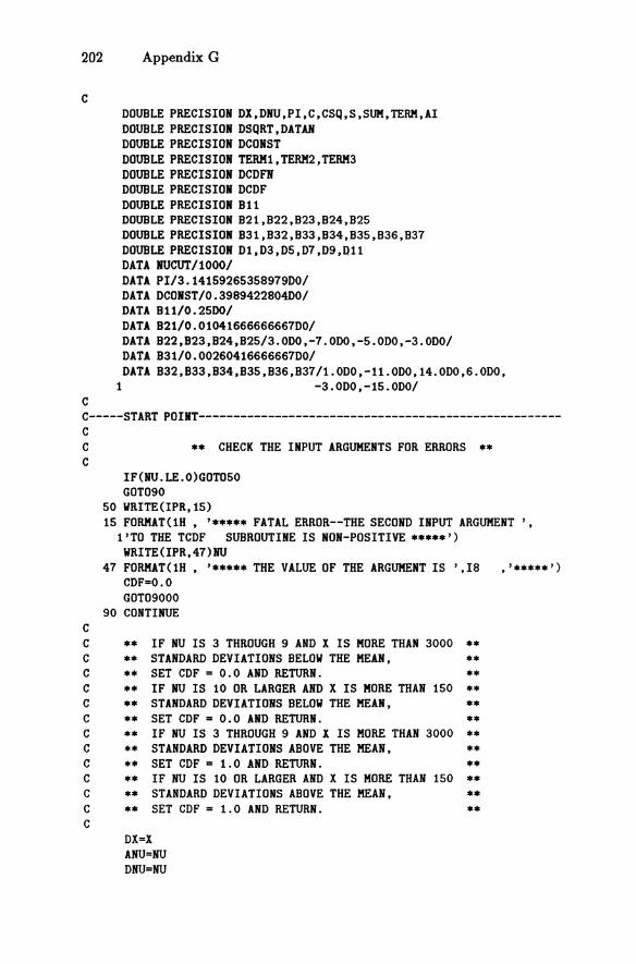
202 Appendix G
C
C
DOUBLE PRECISION DX,DHU,PI,C,CSQ,S,SUM,TERK,AI DOUBLE PRECISION DSQRT,DATAH DOUBLE PRECISION DCONST DOUBLE PRECISION TERK1,TERK2,TERK3 DOUBLE PRECISION DCDFN DOUBLE PRECISION DCDF DOUBLE PRECISION 811 DOUBLE PRECISION 821,822,823,824,825 DOUBLE PRECISION 831,832,833,834,835,836,837 DOUBLE PRECISION Dl,D3,D5,D7,D9,Dll DATA HUCUT/I000/ DATA PI/3.14159265358979DO/ DATA DCONST/0.3989422804DO/ DATA 811/0.25DO/ DATA 821/0.01041666666667DO/ DATA 822,823,824,825/3.0DO,-7.0DO,-5.0DO,-3.0DO/ DATA 831/0.00260416666667DO/ DATA 832,833,834,835,836,837/1.0DO,-11.0DO,14.0DO,6.0DO,
1 -3.0DO,-15.0DO/
C-----START POINT-----------------------------------------------------C C C
C C C C C C C C C C C C C C
** CHECK THE INPUT ARGUMENTS FOR ERRORS **
IF(HU.LE.0)GOT050 GOT090
50 WRITE(IPR,15) 15 FORKAT(lH , '***** FATAL ERROR--THE SECOND INPUT ARGUMENT'
l'TO THE TCDF SUBROUTINE IS NON-POSITIVE *****') WRITE(IPR,47)HU
47 FORKAT(lH , '***** THE VALUE OF THE ARGUMENT IS ',18 ,'*****') CDF=O.O GOT09000
90 CONTINUE
** IF HU IS 3 THROUGH 9 AND 1 IS KORE THAN 3000 ** STANDARD DEVIATIONS 8ELOW THE MEAN, ** SET CDF = 0.0 AND RETURN. ** IF HU IS 10 OR LARGER AND X IS KORE THAN 150 ** STANDARD DEVIATIONS 8ELOW THE MEAN, ** SET CDF = 0.0 AND RETURN. ** IF HU IS 3 THROUGH 9 AND X IS KORE THAN 3000 ** STANDARD DEVIATIONS A80VE THE MEAN, ** SET CDF = 1.0 AND RETURN. ** IF HU IS 10 OR LARGER AND X IS KORE THAN ** STANDARD DEVIATIONS A80VE THE MEAN, ** SET CDF = 1.0 AND RETURN.
Dl=1 ANU=NU DHU=NU
150
** ** ** ** ** ** ** ** ** ** ** **
C
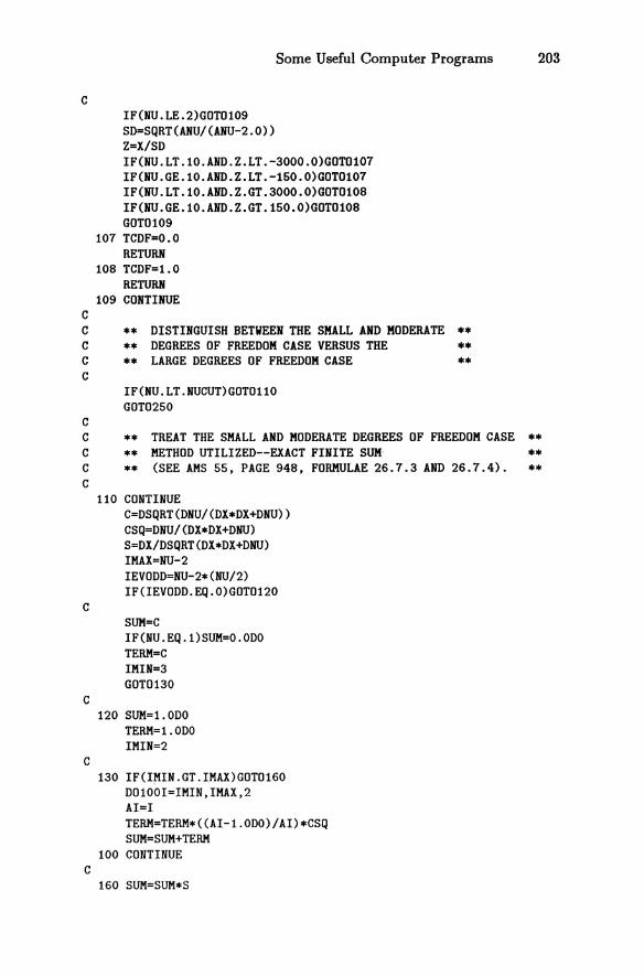
C
IF(NU.LE.2)GOT0109 SD=SQRT(ANU/(ANU-2.0»
Some Useful Computer Programs 203
Z=X/SD IF(NU.LT.l0.AND.Z.LT.-3000.0)GOT0107 IF(NU.GE.l0.AND.Z.LT.-150.0)GOT0107 IF(NU.LT.l0.AND.Z.GT.3000.0)GOT0108 IF(NU.GE.l0.AND.Z.GT.150.0)GOT0108 GOT0109
107 TCDF=O.O RETURN
108 TCDF=1.0 RETURN
109 CONTINUE
C ** DISTINGUISH BETWEEN THE SMALL AND MODERATE ** C C C
C
** DEGREES OF FREEDOM CASE VERSUS THE ** LARGE DEGREES OF FREEDOM CASE
IF(NU.LT.NUCUT)GOTOll0 GOT0250
** **
C ** TREAT THE SMALL AND MODERATE DEGREES OF FREEDOM CASE ** C ** METHOD UTILIZED--EXACT FINITE SUM ** C ** (SEE AMS 55, PAGE 948, FORMULAE 26.7.3 AND 26.7.4). ** C
C
C
C
C
110 CONTINUE C=DSQRT(DNU/(DX*DX+DNU» CSQ=DNU/(DX*DX+DNU) S=DX/DSQRT(DX*DX+DNU) IMAX=NU-2 IEVODD=NU-2*(NU/2) IF(IEVODD.EQ.0)GOT0120
SUM=C IF(NU.EQ.l)SUM=O.ODO TERM=C IMIN=3 GOT0130
120 SUM=1. ODO TERM=1.0DO IMIN=2
130 IF(IMIN.GT.IMAX)GOT0160 D0100I=IMIN,IMAX,2 AI=I TERM=TERM*«AI-l.0DO)/AI)*CSQ SUM=SUM+TERM
100 CONTINUE
160 SUM=SUM*S
204 Appendix G
C
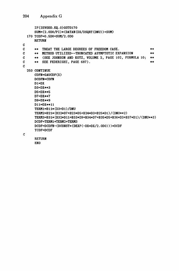
IF(IEVODD.EQ.O)GOT0170 SUK=(2.0DO/PI)*(DATAN(DX/DSQRT(DNU»+SUK)
170 TCDF=0.5DO+SUM/2.0DO RETURN
C ** TREAT THE LARGE DEGREES OF FREEDOM CASE. ** C ** METHOD UTILIZED--TRUNCATED ASYMPTOTIC EXPANSION ** C ** (SEE JOHNSON AND KOTZ, VOLUME 2, PAGE 102, FORMULA 10; ** C ** SEE FEDERIGHI, PAGE 687). ** C
C
250 CONTINUE CDFN=GAUCDF(X) DCDFN=CDFN Dl=DX D3=DX**3 D5=DX**5 D7=DX**7 D9=DX**9 Dl1=DX**l1 TERM1=Bll*(D3+Dl)/DNU TERM2=B21*(B22*D7+B23*D5+B24*D3+B25*Dl)/(DNU**2) TERM3=B31*(B32*Dll+B33*D9+B34*D7+B35*D5+B36*D3+B37*Dl)/(DNU**3) DCDF=TERM1+TERM2+TERM3 DCDF=DCDFN-(DCONST*(DEXP(-DX*DX/2.0DO»)*DCDF TCDF=DCDF
RETURN END
S<.>me Useful Computer Programs 205
SUBROUTINE CORLIB(R3,ELT,RC) C THIS SUBROUTINE APPLIES THE LIBRATION CORRECTION TO AN ATOM C WHOSE POSITION IS DEFINED, WITH RESPECT TO THE ORIGIN OF A C RIGID BODY, BY THE VECTOR RC, WHICH IS A THREE DIMENSIONAL C VECTOR WITH UNITS OF LENGTH. THE TRUE, EQUILIBRIUM POSITION OF C THE ATOM IS RETURNED IN THE THREE DIMENSIONAL VECTOR R3. EL IS C THE LIBRATION TENSOR. IT IS A 3X3 MATRIX, AND HAS UNITS OF C RADIANS**2.
DIMENSION R3(3,3),ELT(3,3),RC(3),ACON(3,3),BCON(3) DO 30 1=1,3 BCON(I)=RC(I) DO 30 J=1,3
30 ACON(I,J)=O. 40 DO 50 1=1,3
DO 50 J=1,3 50 ACON(I,J)=ACON(I,J)+EIJ(ELT,I,J)
CALL SOLVE(ACON,BCON,R3) RETURN END
FUNCTION EIJ(EL,I,J) DIMENSION EL(3,3) IF(I.EQ.J)GO TO 20 EIJ=.5*EL(I,J)-(1./24.)*(EL4(EL,I,1,1,J)+EL4(EL,I,2,2,J)+EL4(EL,
1 I,3,3,J» RETURN
20 K=MOD(I,3)+1 L=MOD(I+1,3)+1 EIJ=1.-.5*(EL(K,K)+EL(L,L»+(1./24.)*(EL4(EL,I,I,K,K)+EL4(EL,I,I,
1 L,L)+3.*(EL(K,K)**2+EL(L,L)**2)+2.*EL4(EL,K,K,L,L» RETURN END
FUNCTION EL4(EL,I,J,K,L) DIMENSION EL(3,3) EL4=EL(I,J)*EL(K,L)+EL(I,K)*EL(J,L)+EL(I,L)*EL(J,K) RETURN END
SUBROUTINE SOLVE(A,B,C) DIMENSION A(3,3),B(3),C(3) DELTA=DETERM(A(1,1),A(1,2),A(1,3» C(1)=DETERM(B(1),A(1,2),A(1,3»/DELTA C(2)=DETERM(A(l,l),B(1),A(1,3»/DELTA C(3)=DETERM(A(l,l),A(1,2),B(1»/DELTA RETURN END
206 Appendix G
FUNCTION DETERK(C1,C2,C3) DIMENSION C1(3) ,C2(3) ,C3(3) DETERK=C1(1)*C2(2)*C3(3)+C1(2)*C2(3)*C3(1)+C1(3)*C2(1)*C3(2)
1 -C1(3)*C2(2)*C3(1)-C1(2)*C2(1)*C3(3)-C1(1)*C2(3)*C3(2) RETURN END
FUNCTION SKTLS(R,I,J,T,EL,S) DIMENSION R(3) ,T(3 ,3) ,EL(3 ,3) ,S(3, 3),RR(3) B(I1,I2,I3)=BIJK(RR,I1,I2,I3) C(I1,I2,I3,I4)=CIJKL(RR,I1,I2,I3,I4) DO 5 M=1,3
5 RR(M)=R(M) SUM=T(I, J) DO 10 K=l,3 SUM=SUM+AIJ(R,J,K)*S(K,I)+AIJ(R,I,K)*S(K,J) DO 10 L=l,3 SUM=SUM+AIJ(R,I,K)*AIJ(R,J,L)*EL(K,L) DO 10 M=l,3 SUM=SUM+3. *EL(L,M) *(S(K ,I)*C (J ,K,L ,M)+S(K ,J)*C(I ,K, L ,M» DO 10 N=1,3
10 SUM=SUM+EL(K,L)*EL(M,N)*(3.*(AIJ(R,I,K)*C(J,L,M,N)+AIJ(R,J,K) 1 *C(I,L,M,N»+2.*B(I,K,M)*B(J,L,N»
SKTLS=SUM RETURN END
FUNCTION D2KDT(I,J,K,L) D2KDT=0. IF(I.EQ.K.AND.J.EQ.L)D2KDT=1. RETURN END
Some Useful Computer Programs 207
FUNCTION D2KDL(R,EL,S,I,J,K,L) DIMENSION R(3),EL(3,3),S(3,3),RR(3) C(I,J,K,L)=CIJKL(RR,I,J,K,L) C6(I,K,L,M)=6.*C(I,K,L,M) ACC(I,J,K,L,M,N)=3.*AIJ(RR,I,K)*C(J,L,M,N) DO 10 M=l,3
10 RR(M)=R(M) SUM=AIJ(R,I,K)*AIJ(R,J,L)+AIJ(R,I,L)*AIJ(R,J,K) DO 1000 M=l,3 SUM=SUM+S(M,I)*C6(J,K,L,M)+S(M,J)*C6(I,K,L,M) DO 1000 N=l,3 SUM=SUM+EL(M,N)*(ACC(I,J,K,L,M,N)+ACC(I,J,L,K,M,N)+ACC(J,I,K,L,M,N
1 )+ACC(J,I,L,K,M,N)+ACC(I,J,M,N,K,L)+ACC(J,I,M,N,K,L)+ACC(I,J 2 ,M,N,L,K)+ACC(J,I,M,N,L,K)+4.*(BIJK(R,I,K,M)*BIJK(R,J,L,N)+ 3 BIJK(R,I,L,M)*BIJK(R,J,K,N»)
1000 CONTINUE D2KDL=SUM IF(K.EQ.L)D2KDL=SUM/2. RETURN END
FUNCTION D2KDS(R,EL,I,J,K,L) DIMENSION R(3),EL(3,3),RR(3) CCC(J,K,L,M)=3.*CIJKL(RR,J,K,L,M) DO 10 M=1,3
10 RR(M)=R(M) SUM=O. IF(I.NE.L)GO TO 1000 SUM=SUM+AIJ(R,J,K) DO 500 M=l,3 DO 500 N=l,3
500 SUM=SUM+EL(M,N)*CCC(J,K,M,N) 1000 IF(J.NE.L)GO TO 2000
SUM=SUM+AIJ(R,I,K) DO 1500 M=l,3 DO 1500 N=l,3
1500 SUM=SUM+EL(M,N)*CCC(I,K,M,N) 2000 D2KDS=SUM
RETURN END
208 Appendix G
FUNCTION TKTLS(R,I,J,K,EL,S) DIMENSION R(3),EL(3,3),S(3,3) INTEGER P SUK=O. DO 1000 L=l,3 DO 1000 M=l,3 SUK=SUK+2.*(S(L,I)*S(M,J)*BIJK(R,K,L,M)
1 +S(L,I)*S(M,K)*BIJK(R,J,L,M) 2 +S(L,J)*S(M,K)*BIJK(R,I,L,M»
DO 1000 N=l,3 SUK=SUK+2.*EL(M,N)*
1 (S(L,I)*(AIJ(R,J,M)*BIJK(R,K,L,N)+AIJ(R,K,M)*BIJK(R,J,L,N» 2 +S(L, J) *(AIJ (R,I ,M) *BIJK(R,K, L ,N)+AIJ (R,K ,'O*BIJK(R, I ,L,N» 3 +S(L ,K)*(AIJ(R, I,M) *BIJK(R, J ,.L,N)+AIJ(R, J ,M)*BIJK(R, I ,L ,N»)
DO 1000 P=l,3 SUK=SUK+EL(N,P)*(S(L,J)*S(M,K)*PIJKLM(R,I,L,M,N,P)+S(L,I)*S(M,K)*
1 PIJKLM(R,J,L,M,N,P)+S(L,I)*S(M,J)*PIJKLM(R,K,L,M,N,P) 2 +2.*EL(L,M)*(AIJ(R,I,L)*AIJ(R,J,N)*BIJK(R,K,M,P) 3 +AIJ(R,I,L)*AIJ(R,K,N)*BIJK(R,J,M,P) 4 +AIJ(R,J,L)*AIJ(R,K,N)*BIJK(R,I,M;P»)
1000 CONTINUE TKTLS=SUK RETURN END
FUNCTION D3KDL(R,EL,S,I,J,K,L,M) DIMENSION R(3),EL(3,3),S(3,3),RR(3) INTEGER P ABB(J,K,L,M,N)=2.*AIJ(RR,J,L)*BIJK(RR,K,M,N) AAB(I,J,K,L,M,N,NN)=AIJ(RR,I,L)*AIJ(RR,J,N)*BIJK(RR,K,M,NN) PP(I,J,K,L,M)=PIJKLM(RR,I,J,K,L,M)+PIJKLM(RR,I,J,K,M,L) DO 10 N=l,3
10 RR(N)=R(N) SUK=O. DO 1000 N=l,3 SUK=SUK+S(N,I)*(ABB(J,K,L,M,N)+ABB(K,J,L,M,N)+ABB(J,K,M,L,N)+ABB(K
1 ,J,M,L,N»+S(N,J)*(ABB(I,K,L,M,N)+ABB(K,I,L,M,N)+ABB(I,K,M,L,N 2 )+ABB(K,I,M,L,N»+S(N,K)*(ABB(I,J,L,M,N)+ABB(J,I,L,M,N)+ABB(I, 3 J,M,L,N)+ABB(J,I,M,L,N»
DO 1000 P=l,3 SUK=SUK+S(N,J)*S(P,K)*PP(I,N,P,L,M)+S(N,I)*S(P,K)*PP(J,N,P,L,M)
1 +S(N,I)*S(P,J)*PP(K,N,P,L,M)+2.*EL(N,P)*(AAB(I,J,K,L,M,N,P) 2 +AAB(I,K,J,L,M,N,P)+AAB(J,K,I,L,M,N,P)+AAB(I,J,K,N,P,L,M) 3 +AAB(I,K,J,N,P,L,M)+AAB(J,K,I,N,P,L,M»
1000 CONTINUE D3KDL=SUK IF(L.EQ.M)D3KDL=SUK/2. RETURN END
Some Useful Computer Programs 209
FUNCTION D3KDS(R,EL,S,I,J,K,LP,MP) DIMENSION R(3),EL(3,3),S(3,3),RR(3) INTEGER P BB(K,L,M)=2.*BIJK(RR,K,L,M) ABB(J,K,L,M,N)=2.*AIJ(RR,J,L)*BIJK(RR,K,M,N) DO 10 M=1,3
10 RR(M)=R(M) SUM=O. DO 1000 L=1,3 DO 1000 H=1,3 IF(L.EQ.LP.AND.I.EQ.HP)SUM=SUM+S(M,J)*BB(K,L,M)+S(M,K)*BB(J,L,H) IF(M.EQ.LP.AND.J.EQ.MP)SUM=SUM+S(L,I)*BB(K,L,M) IF(M.EQ.LP.AND.K.EQ.MP)SUM=SUM+S(L,I)*BB(J,L,M)+S(L,J)*BB(I,L;M) IF(L.EQ.LP.AND.J.EQ.HP)SUM=SUM+S(H,K)*BB(I,L,M) DO 1000 N=1,3 IF(L.NE.LP)GO TO 500 IF(I.EQ.HP)SUM=SUM+EL(M,N)*(ABB(J,K,M,L,N)+ABB(K,J,M,L,N» IF(J.EQ.HP)SUM=SUM+EL(M,N)*(ABB(I,K,M,L,N)+ABB(K,I,M,L,N» IF(K.EQ.HP)SUM=SUM+EL(M,N)*(ABB(I,J,M,L,N)+ABB(J,I,M,L,N»
500 DO 1000 P=1,3 IF(L.NE.LP)GO TO 750 IF(J.EQ.HP)SUM=SUM+EL(N,P)*S(M,K)*PIJKLM(R,I,L,M,N,P) IF(I.EQ.HP)SUM=SUM+EL(N,P)*(S(M,K)*P1JKLM(R,J,L,M,N,P)+S(M,J)*
1 P1JKLM(R,K,L,M,N,P» 750 IF(M.NE.LP)GO TO 1000
IF(K.EQ.MP)SUM=SUM+EL(N,P)*(S(L,J)*P1JKLM(R,1,L,M,N,P)+S(L,1)* 1 P1JKLM(R,J,L,M,N,P» 1F(J.EQ.HP)SUM=SUM+EL(N,P)*S(L,1)*P1JKLM(R,K,L,M,N,P)
1000 CONTINUE D3KDS=SUM RETURN END
210 Append~G
SUBROUTINE EULER (PHI ,CHI ,OMEGA ,TRANS) C SUBROUTINE TO GENERATE THE MATRIX B-INVERSE FROM THE EULERIAN C ANGLES PHI ,CHI ,AND OMEGA. OMEGA IS THE ANGLE (IN DEGREES) BY C WHICH A SPECIAL, ORTHONORMAL COORDINATE SYSTEM MUST BE ROTATED, C CLOCKWISE AS VIEWED DOWN THE POSITIVE Z AXIS OF A 'STANDARD' C REFERENCE COORDINATE SYSTEM, IN ORDER TO BRING THE Z AXIS OF THE C SPECIAL SYSTEM INTO THE X - Z PLANE OF THE STANDARD SYSTEM. CHI C IS THE ANGLE (IN DEGREES) BY WHICH THE SPECIAL SYSTEM MUST BE C ROTATED CLOCKWISE ABOUT THE Y AXIS OF THE STANDARD SYSTEM TO C BRING THE Z AXES OF THE TWO COORDINATE SYSTEMS INTO COINCIDENCE. C PHI IS THE ANGLE (IN DEGREES) OF A CLOCKWISE ROTATION ABOUT THE C COKMON Z AXES TO BRING THE TWO COORDINATE SYSTEMS INTO COIN-C CIDENCE. ENTRIES DTDPHI, DTDCHI, AND DTDOMG GIVE THE MATRICES C WHOSE ELEMENTS ARE THE DERIVATIVES OF THE EULER MATRIX WITH C RESPECT TO PHI, CHI, AND OMEGA.
DATA RAD/57.2957792/ DIMENSION TRANS(3,3) ASSIGN 10 TO KGO GO TO 100
10 TRANS(l,l)=CP*CX*CO-SP*SO TRANS(2,1)=CP*CX*SO+SP*CO TRANS(3,1)=-CP*SX TRANS(1,2)=-SP*CX*CO-CP*SO TRANS(2,2)=-SP*CX*SO+CP*CO TRANS(3,2)=SP*SX TRANS(1,3)=SX*CO TRANS (2,3)=SX*SO TRANS (3,3)=CX RET~N
ENTRY DTDPHI(PHI,CHI,OMEGA,TRANS) ASSIGN 20 TO KGO GO TO 100
20 TRANS(l,l)=(-SP*CX*CO-CP*SO)/RAD TRANS(2,1)=(-SP*CX*SO+CP*CO)/RAD TRANS(3,1)=SP*SX/RAD TRANS(1,2)=(-CP*CX*CO+SP*SO)/RAD TRANS (2,2)=(-CP*CX*SO-SP*CO)/RAD TRANS(3,2)=CP*SX/RAD DO 25 1=1,3
25 TRANS(I,3)=0. RE~N
ENTRY DTDCHI(PHI,CHI,OMEGA,TRANS) ASSIGN 30 TO KGO GO TO 100
30 TRANS(l,l)=-CP*SX*CO/RAD TRANS(2,1)=-CP*SX*SO/RAD TRANS(3,1)=-CP*CX/RAD TRANS(1,2)=SP*SX*CO/RAD TRANS (2,2)=SP*SX*SO/RAD TRANS(3,2)=SP*CX/RAD TRANS(1,3)=CX*CO/RAD TRANS (2, 3)=CX*SO/RAD
TRANS(3,3)=-SX/RAD RETURN
Some Useful Computer Programs 211
ENTRY DTDOKG(PHI,CHI,OHEGA,TRANS) ASSIGN 40 TO KGO GO TO 100
40 TRANS(l,l)=(-CP*CX*SO-SP*CO)/RAD TRANS(2,l)=(CP*CX*CO-SP*SO)/RAD TRANS(l,2)=(SP*CX*SO-CP*CO)/RAD TRANS (2 ,2)=(-SP*CX*CO-CP*SO)/RAD TRANS(l,3)=-SX*SO/RAD TRANS(2,3)=S~*COIRAD DO 45 1=1,3
45 TRANS(3,I)=O. RETURN
100 CP=COS(PHI/RAD) CX=COS(CHI/RAD) CO=COS(OKEGA/RAD) SP=SIN(PHI/RAD) SX=SIN(CHI/RAD) SO=SIN(OKEGA/RAD) GO TO KGO(10,20,30,40) END
FUNCTION PIJKLK(R,I,J,K,L,K) DIMENSION R(3) PIJKLK=12.*DIJKLK(R,I,J,K,L,M) RETURN END
212 Appendix G
FUNCTION AIJ(R,I,J) DIMENSION R(3) GO TO (10,20,30),1
10 GO TO (100,200,300),J 20 GO TO (300,100,200),J 30 GO TO (200,300,100),J 100 AIJ=O.
RETURN 200 MH=HOD(I+l,3)+1
AIJ=R(MH) RETURN
300 MH=HOD(I,3)+1 AIJ=-R(MH) RETURN END
FUNCTION BIJK(R,I,JJ,KK) DIMENSION R(3) DIV=2. IF(JJ.EQ.KK)DIV=l. J=MINO(JJ,KK) K=HAXO(JJ,KK) GO TO (10,20,30),1
10 GO TO (12,14,400),J 12 GO TO (100,200,300),K 14 IF(K-2)400,400,100 20 GO TO (22,24,400),J 22 GO TO (400,300,100),K 24 IF(K-2)100,100,200 30 GO TO (32,34,100),J 32 GO TO (400,100,200),K 34 IF(K-2)400,400,300 100 BIJK=O.
RETURN 200 MH=MOD(I,3)+1
BIJK=.5*R(MH)/DIV RETURN
300 MH=MOD(I+l,3)+1 lIJK=.5*R(MH)/DIV .tETURN
400 BIJK=-.5*R(I)/DIV RETURN END
Some Useful Computer Programs 213
FUNCTION CIJKL(R,I,JJ,KK,LL) DIMENSION R(3) IF(JJ.EQ.KK.AND.JJ.EQ.LL)GO TO 7 IF(JJ.NE.KK.AND.JJ.NE.LL.AND.KK.NE.LL)GO TO 8 IF(JJ-KK)1,2,3
1 J=JJ L=KK K=LL GO TO 4
2 J=MINO(JJ,LL) K=KK L=MAXO (J J , LL) GO TO 4
3 J=KK K=LL L=JJ
4 DIV=3. GO TO 9
7 J=JJ K=JJ L=JJ DIV=l. GO TO 9
8 J=l. K=2 L=3 DIV=6.
9 GO TO (10,20,30),1 10 GO TO (12,15,300),J 12 GOTO (13,100,100),K 13 GO TO (100,200,300),L 15 IF(K-2)16,16,200 16 IF(L-2)200,200,300 20 GO TO (22,25,200),J 22 GOTO (23,24,300),K 23 GO TO (300,100,200),L 24 IF(L-2)300,300,100 25 IF(K-2)26,26,100 26 IF(L-2)100,100,200 30 GO TO (32,35,100),J 32 GO TO (33,34,200),K 33 GO TO (200,300,100),L 34 IF(L-2)200,200,100 35 IF(K-2)36,36,300 36 IF(L-2)300,300,100 100 CIJKL=O.
RETURN 200 MM=MOD(I+1,3)+1
CIJKL=-R(MM)/(6.*DIV) RETURN
300 MM=MOD(I,3)+1 CIJKL=R(MM)/(6.*DIV)

214 Appendix G
RETURN END
Some Useful Computer Programs 215
FUNCTION DIJKLM(R,I,JI,KI,LI,MI) DIMENSION R(3) IN=JhKI*LI*MI IF(MOD(IN,6).EQ.0.AND.IN.LE.18)GO TO 1080 IF(IN.EQ.4.0R.IN.EQ.9.0R.IN.EQ.36)GO TO 1060 IF(JI.NE.KI.OR.KI.HE.LI.OR.LI.NE.MI)GO TO 1040 DIV=l. GO TO 1100
1040 DIV=4. GO TO 1100
1060 DIV=6. GO TO 1100
1080 DIV=12. 1100 IF(MOD(IN,3).HE.0)GO TO 1500
M=3 IN=IN/3 IF(MOD(IN,3).HE.0)GO TO 1250 L=3 IN=IN/3 IF(MOD(IN,3).HE.0)GO TO 1125 K=3 J=IN/3 GO TO 1900
1125 IF(MOD(IN,2).NE.0)GO TO 1150 K=2 J=IN/2 GO TO 1900
1150 K=l J=l GO TO 1900
1250 IF(MOD(IN,2).NE.0)GO TO 1375 L=2 IN=IN/2 IF(MOD(IN,2).NE.0)GO TO 1150 K=2 J=IN/2 GO TO 1900
1375 L=l GO TO 1150
1500 IF(MOD(IN,2).NE.0)GO TO 1750 M=2 IN=IN/2 GO TO 1250
1750 M=l GO TO 1375
1900 GO TO (100,200,300),1 100 GO TO (110,150,2000),J 110 GO TO (120,140,3000),K 120 GO TO (125,130,2000),L 125 GO TO (1000,4000,3000),M 130 IF(M-2) 1000,2000,1000 140 IF(L-2) 1000,145,4000
216 Appendix G
145 IF(K-2) 1000,4000,3000 150 IF(K-2) 1000, 160, 1000 160 IF(L-2) 1000,170,5000 170 IF(K-2) 1000,2000,1000 200 GO TO (210,250,2000),J 210 GO TO (220,240,1000),K 220 GO TO (225,230,5000),L 225 GO TO (2000,3000,1000),K 230 IF(K-2) 1000,2000,4000 240 IF(L-2) 1000,245,3000 245 IF(K-2) 1000,3000,1000 250 IF(K-2) 1000,260,4000 260 IF(L-2) 1000,270,2000 270 IF(K-2) 1000,1000,4000 300 GO TO (310,350,1000),J 310 GO TO (320,340,4000),K 320 GO TO (325,330,2000),L 325 GO TO (2000,1000,4000),K 330 IF(K-2) 1000,5000,3000 340 IF(L-2)1000,345,1000 345 IF(K-2) 1000,1000,4000 350 IF(K-2) 1000,360,3000 360 IF(L-2) 1000,370,2000 370 IF(K-2) 1000,2000,3000 1000 DIJKLK=O.
RETURR 2000 FAC=1. 2010 DIJKLK=FAC$R(I)/(24.$DIV)
RETURN 3000 KK=KOD(I+l,3)+1
3010 DIJKLK=-R(KK)/(24.$DIV) RETURR
4000 KK=KOD(I,3)+1 GO TO 3010
5000 FAC=2. GO TO 2010 ERD
Bibliography
The following list makes no pretense to being inclusive. Some books are current, and some are out of date. Some are classics in their fields, while others are obscure. All contain at least a few pages of useful information.
Ahmed, F. R. (ed.): Crystallographic Computing. Proceedings of the 1969 International Summer School on Crystallographic Computing, Munksgaard, Copenhagen, 1970.
Arndt, U. W., and Willis, B. T. M.: Single Crystal Diffractometry. Cambridge University Press, Cambridge, 1966.
Draper, N., and Smith, H.: Applied Regression Analysis. John Wiley & Sons, New York, London, Sydney, 1966.
Gill, P. E., Murray, W., and Wright, M. H.: Practical Optimization. Academic Press, London, New York, Toronto, Sydney, San Francisco, 1981.
Hamilton, W. C.: Statistics in Physical Science. The Ronald Press Company, New York, 1964.
International Tables for Cryst~ography, published for the International Union of Crystallography by Kluwer Academic Publishers, Dordrecht, Boston, London, 1992.
Kendall, M. G., and Stuart, A.: The Advanced Theory of Statistics, 2nd ed. Charles Griffin & Co., Ltd., London, 1963.
Lide, D. R., Jr., and Paul, M. A. (eds.): Critical Evaluation of Chemical and Physical Structural Information. National Academy of Sciences, Washington, 1974.
Nye, J. F.: Physical Properties of Crystals. Clarendon Press, Oxford, 1957. Pauling, 1., and Wilson, E. B. Jr.: Introduction to Quantum Mechanics. McGraw
Hill Book Company, Inc., New York, London, 1935. Phillips, F. C.: An Introduction to Crystallography. Longmans, Green & Co.,
London, New York, Toronto, 1946. Pipes, 1. A.: Applied Mathematics for Engineers and Physicists. McGraw-Hill
Book Company, Inc., New York and London, 1946. Squires, G. L.: Introduction to the Theory of Thermal Neutron Scattering. Cam
bridge University Press, Cambridge, London, New York, Melbourne, 1978. Stewart, G. W.: Introduction to Matrix Computations. Academic Press, New
York, London, 1973. Tolimieri, R., An, M., and Lu, C.: Algorithms for Discrete Fourier Transform and
Convolution. Springer-Verlag, New York, Heidelberg, Berlin, London, Paris, Tokyo, Hong Kong, 1989.
Widder, D. V.: Advanced Calculus. Prentice-Hall, Inc., New York, 1947. Willis, B. T. M. (ed.): Thermal Neutron Diffraction, Oxford University Press,
Oxford, 1970. Wilson, E. B., Jr., Decius, J. C. and Cross, P. C.: Molecular Vibrations, The The
ory of Infrared and Raman Vibrational Spectra. McGraw-Hill Book Company, Inc., New York, Toronto, London, 1955.
Wooster, W. A.: Crystal Physics. Cambridge University Press, Cambridge, 1949.
Index
Accidental absence, 48 Accuracy, 95, 116 Adjoint of a matrix, 9 Andrews, D. F., 81 Anharmonic forces, 127 Associative law, 3 Asymmetric unit, 46, 152 Atomic displacement factor, 47,
64 Atomic scattering factor, 47, 63,
126 Augmentation, 5 Axial vector, 50, 74, 131
Basis function, 37 Basis vector, 17 Best linear unbiased estimate, 79 Beta function, 168 BFGS algorithm, 90 Bias, 95, 117 Bisecting position, 56 Bloch's theorem, 64, 173 Boltzmann weighting factor, 179 Bragg reflection, 55, 62, 124 Bragg's law, 52 Bravais lattice, 40-41 Broyden-Fletcher-Goldfar b-Shanno
algorithm, 90
Cauchy distribution, 79 Central limit theorem, 101 Character, 24 Characteristic function, 70, 171 Chebychev polynomials, 114 Chemical constraints, 133 X2 distribution, 108, 102 Chinese remainder theorem, 144 Cholesky factor, 11, 18, 55, 64,
121 Circulant matrix, 146
Column vector, 2,49 Commutative law, 3 Conditional probability density func-
tion, 60 Confidence interval, 115 Conic sections, 132 Conjugate gradients, 88 Constrained refinement, 94 Constrained sum of squares, 109 Constraint matrix, 128 Constraints, 127 Contravariance, 59 Contravariant metric tensor, 59 Conventional model, 127 Cooley, J. W., 144 Cooley-Thkey algorithm, 144 Corrected sum of squares, 98 Correction factor, 98 Correlation, 112, 117 Correlation coefficient, 112 Correlation matrix, 112, 119 Covariance, 59, 61 Covariant metric tensor, 59 Cross product, 51 Crystal lattice, 17 Crystal systems, 41 Crystallographic point groups, 24 Cubic equation, 161 Cubic system, 41 Cumulant, 69, 71
in terms of moments, 71 Cumulants, 127 Curvilinear motion, 127
Davidon-Fletcher-Powell algorithm, 90
De Broglie wavelength, 63 Debye-Waller factor, 47 Decomposition, 6 Degenerate eigenvector, 65
Degrees of freedom, 98, 108 Design matrix, 84, 103 Determinant, 2 DFP algorithm, 90 Diagonal matrix, 2 Dimension of a representation, 22 Direct product, 59 Direct product group, 21 Discrete Fourier transform, 141 Dispacement factor tensor, 126 Dot product, 51 Downdating, 91
Edgeworth series, 138 Eigenvalue, 8, 59, 65, 121, 161 Eigenvector, 10, 59, 65, 115, 161 Eigenvectors, 138 Elastic constants, 69, 185 Elasticity, 69 Electric dipole moment, 68, 182 Elephant parameter, 127 Ensemble average, 63 Equatorial circle, 157 Equatorial plane, 157 Ergodic theorem, 63 Estimate, 78
least squares, 99 Estimated standard deviation, 115 Estimator, 96 Euler's theorem, 17, 72 Euler, Lenhard, 16 Eulerian angles, 16, 55, 129 Ewald sphere, 54 Ewald, P. P., 54 Expected value, 63 Extinction, 127
F distribution, 108, 128 F ratio, 109 False minimum, 85, 92 Fast Fourier transform, 140 Field, 147 Finding the minimum, 82 Fitting functions, 77 Form, 56
Index 219
Four-circle diffractometer, 56 Fourier transform, 63, 70, 126, 140,
171 Fourier, J., 140 Fourth-rank tensor, 185 Friedel's law, 150 Fudge factor, 119
Gamma function, 102, 167 Gauss-Markov theorem, 79 Gauss-Newton algorithm, 85 Gaussian density function, 70, 126 Gaussian distribution, 78,101,165 Gaussian distribution function, 60 Gaussian elimination, 6 Gaussian error distribution, 105 Gaussian probabiltiy density func-
tion, 134 General position, 46 Generalized inverse, 5 Gerade,25 Glide plane, 43 Global minimum, 85,93 Good, J., 144 Good-Thomas algorithm, 144 Gossett, W. S., 112 Gradient, 59, 80 Gram-Charlier series, 138 Great circle, 158 Group, 20
cyclic, 21 direct product, 21 point., 22 postulate, 20 space, 23
Group generator, 24
Habit, 56 Hamilton's R-factor ratio test, 129 Hamilton, W. C., 129 Harmonic oscillator, 70 Harmonic potential function, 135 Harmonic potential well, 64, 126 Hermann, C., 44 Hermann-Mauguin notation, 44
220 Index
Hermite polynomials, 134, 177 Hermitian matrix, 9 Hermitian vector, 150 Hessian matrix, 85, 88-89, 112,
115, 128 Hexagonal system, 41
Idempotent, 121 Identity element, 20 Identity matrix, 4 Identity operation, 20 III conditioned, 113, 133 Improper rotation axis, 23 Independent observations, 97 Inner product, 51 Integrated area, 124 Interatomic vector, 59 Inverse, 20 Inverse of a matrix, 4 Inversion, 20 Irreducible representation, 22 Isotropic temperature factor, 65 Iteratively reweighted least squares,
82
Joint distribution, 78 Joint probability density function,
60
Kronecker delta function, 4 Kurtosis, 72, 138
Lack of fit, 117 Lack-of-fit sum of squares, 108 Lagrange undetermined multipli-
ers, 128 Lattice
body-centered, 41 face-centered, 41 rhombohedral, 41 single-face-centered, 41
Least squares Hessian matrix, 104 mean plane, 133 method of, 105
Least squares estimate, 99 Leverage, 121 Libration correction, 132 Libration tensor, 74 Likelihood, 77 Likelihood function, 78 Line search, 87 Linear combinations, 115 Linear model, 103 Linear transformations, 14 Linearly dependent, 86 Linearly independent, 113 Lorentz factor, 125 Lower triangular matrix, 2
Magnitude, 49 Marginal distribution, 78 Marginal probability density func-
tion, 60 Matrix, 1
adjoint, 9 circulant, 146 dense, 141 diagonal, 2 Hermitian, 9 identity, 4 inverse, 4-5 lower triangular, 2 null, 2 orthogonal, 10 positive definite, 11 singular, 4-5 skew circulant, 146 sparse, 142 square, 2 symmetric, 161 unitary, 10 upper triangular, 2
Mauguin, C., 44 Mean, 60, 96, 124 Mean square displacement, 63
sample, 96 weighted, 99
Median absolute value, 106 Meridian of longitude, 157
Method of least squares, 78 Metric tensor, 17 Miller indices, 52 Minor of a determinant, 3 Mirror refiection, 20 Molecular symmetry, 129 Moment, 69-70
in terms of cumulants, 71 of the normal distribution, 167
Moments, 127, 137 Monoclinic system, 41 Multiplication of matrices, 3 Multiplication table, 21
Newton's method, 82 Normal distribution, 101, 165 Normal equations matrix, 85 Normal error distribution, 105 Normalization factor, 60, 165 Notation
Hermann-Mauguin, 44 Schonfiies, 44
Null matrix, 2
Obverse setting, 41 Orbit, 152 Orbit exchange, 153 Orientation matrix, 54-55 Orthogonal, 51, 88 Orthogonal matrix, 10 Orthogonal transformation, 60 Orthonormal, 161 Orthonormal coordinate system,
13,38 Orthorhombic system, 41 Outliers, 80
Parallel of latitude, 158 Partition, 5 Pawley, G. S., 127 Penalty function, 94 Piezoelectric constants, 182 Piezoelectric moduli, 182 Piezoelectricity, 68 Planck's constant, 173
Index 221
Point group, 22 Poisson distribution, 124 Polar vector, 49,74 Polarization factor, 125 Population variance, 97 Positive definite, 86, 113 Positive definite matrix, 11 Power series, 114 Precision, 95, 116 Prime number, 145 Principal axes, 65 Probability density function, 63,
96, 173 Probability integral, 165 Projection matrix, 120 Propagation vector, 126 Proper rotation axis, 23
Quasi-Newton methods, 90
Rader field algorithm, 147 Rader, C. M., 147 Raw sum of squares, 98 Real space metric tensor, 18 Reciprocal lattice, 52, 126 Reciprocal space metric tensor, 18 Recursion relation, 174 Reducible representation, 22 Relative variance, 100 Replication sum of squares, 108 Representation, 21
faithful, 21 fully symmetric, 26 irreducible, 22, 25 reducible, 22
Resistance, 80 Restrained refinement, 94 Reverse setting, 41 Rhombic dodecahedron, 56 Right-handed rotation, 44 Rigid body motion, 127 Rigid body motion tensor, 74, 131 Robust/resistant procedure, 80
algorithms, 106 Robustness, 80
222 Index
Rotation, 20 Rotation axis
improper, 23 proper, 23
Rotation of axes, 14 Row vector, 2', 49 Row-column method, 149
S tensor, 181 Saddle point, 85 Sample mean, 96 Scalar product, 51 Scale factor, 125 Scatter plot, 117 Scattering density, 126 Schonfiies, A. M., 21-22
notation, 44, 21-22 Schrodinger's equation, 135, 173 Schwarz's inequality, 86, 113 Screw axis, 43 Screw correlation tensor, 74 Second-rank tensor, 181 Shape constraints, 129 Similarity transformation, 10, 38 Singular matrix, 4 Skew circulant matrix, 146 Skewness, 72 Small circle, 157 Sorting algorithm, 106 Space group, 23, 41 Space group symmetry
in Fourier transforms, 152 Space lattice, 40 Special position, 48 Square matrix, 2 Standard deviation, 62 Standard orthonormal coordinate
system, 17, 130 Standard uncertainty, 115 Standardized residual, 117 Static disorder, 127 Stationary point, 93 Statistic, 96 Statistically independent, 61, 117
Statistically uncorrelated observa-tions, 125
Steepest descents, 87 Stereographic projection, 24, 157 Strain, 67 Stress, 67 Structure amplitude, 62, 126 Structure factor, 62, 69, 126 Student (W. S. Gossett), 112 Student's t dsitribution, 112 Subgroup, 21, 37
isomorphic, 48 non-isomorphic, 48
Sublattice, 57, 163 Sum of squared residuals, 98 Summing convention, 3 Supergroup, 21, 37 Superiattice, 57, 163 Symmetry, 20 Systematic absence, 48 Systematic error, 95
Table character, 24
Taylor's series, 70, 88, 115, 135 Temperature factor, 47 Tensor, 58
anisotropic displacement fac-tor, 162
fourth rank, 69 second rank, 58 third rank, 68
Tensor product, 143 Tetragonal system, 41 Thermal ellipsoid, 162 Thermal ellipsoids, 64 Third-rank tensor, 182 Thomas, L. H., 144 Thomson electron, 126 Time average, 63 Trace of a matrix, 2 Trace-of-S singularity, 132 Transcendental, 93 Translation, 20 Translation group, 43
Translation tensor, 74 Transpose of a matrix, 2 Trapezoidal rule, 141 Triclinic system, 41 Trigonal system, 41 Trivariate Gaussian probability den
sity function, 138 Tukey, J. W., 81, 144 Twiddle factor, 144
Uncertainty, 120 Uncorrected sum of squares, 98 Ungerade, 25 Unit cell, 41 Unit group, 146 Unitary matrix, 10, 38 Update formula, 90 Upper triangular matrix, 2
Variance, 60, 78, 96, 124 of the integrated intensity, 125 population, 97
Variance-covariance matrix, 60, 97, 104, 112, 115, 120, 128, 138
Vector of differences, 128 Vector product, 51
axial, 50 column, 2, 49 polar, 49 row, 2, 49
Wave function, 173, 175 Weight, 99 Weighted mean, 99 Weighted R index, 129 Winograd algorithms, 148 Winograd, S., 148 Wulf net, 158
Zone axis, 56 Zones, 56
Index 223


![STEREOGRAPHIC MAP PROJECTION OF CROATIA...CROATIA The stereographic projection has not been previously considered for the region of Croatia. A. Fashing [12] considered it for the area](https://img.pdfslide.net/doc/110x75/60c3cc2e11a4af2d2d1b5dae/stereographic-map-projection-of-croatia-croatia-the-stereographic-projection.jpg)