APPENDIX Outsourcing Tasks Online: Matching Supply … · APPENDIX Outsourcing Tasks Online: Matching Supply and Demand on Peer-to-Peer Internet Platforms Zo¨e Cullen and Chiara

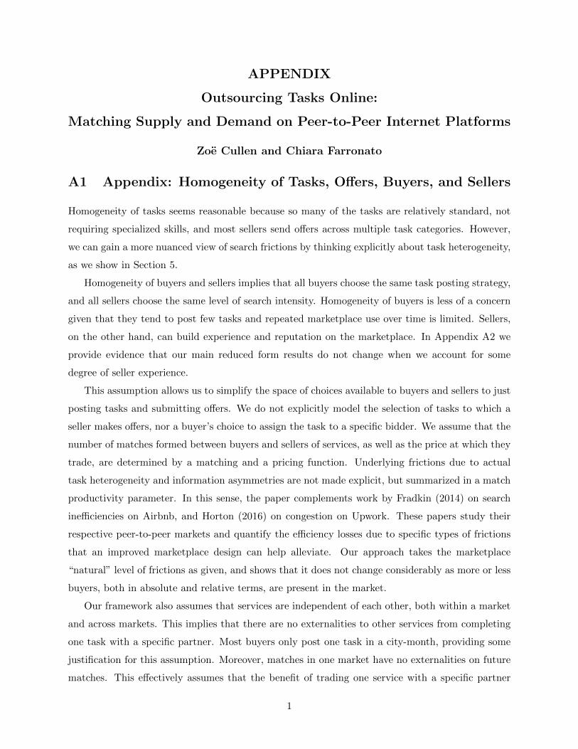
APPENDIX

Outsourcing Tasks Online:

Matching Supply and Demand on Peer-to-Peer Internet Platforms

Zoe Cullen and Chiara Farronato

A1 Appendix: Homogeneity of Tasks, O↵ers, Buyers, and Sellers

Homogeneity of tasks seems reasonable because so many of the tasks are relatively standard, not

requiring specialized skills, and most sellers send o↵ers across multiple task categories. However,

we can gain a more nuanced view of search frictions by thinking explicitly about task heterogeneity,

as we show in Section 5.

Homogeneity of buyers and sellers implies that all buyers choose the same task posting strategy,

and all sellers choose the same level of search intensity. Homogeneity of buyers is less of a concern

given that they tend to post few tasks and repeated marketplace use over time is limited. Sellers,

on the other hand, can build experience and reputation on the marketplace. In Appendix A2 we

provide evidence that our main reduced form results do not change when we account for some

degree of seller experience.

This assumption allows us to simplify the space of choices available to buyers and sellers to just

posting tasks and submitting o↵ers. We do not explicitly model the selection of tasks to which a

seller makes o↵ers, nor a buyer’s choice to assign the task to a specific bidder. We assume that the

number of matches formed between buyers and sellers of services, as well as the price at which they

trade, are determined by a matching and a pricing function. Underlying frictions due to actual

task heterogeneity and information asymmetries are not made explicit, but summarized in a match

productivity parameter. In this sense, the paper complements work by Fradkin (2014) on search

ine�ciencies on Airbnb, and Horton (2016) on congestion on Upwork. These papers study their

respective peer-to-peer markets and quantify the e�ciency losses due to specific types of frictions

that an improved marketplace design can help alleviate. Our approach takes the marketplace

“natural” level of frictions as given, and shows that it does not change considerably as more or less

buyers, both in absolute and relative terms, are present in the market.

Our framework also assumes that services are independent of each other, both within a market

and across markets. This implies that there are no externalities to other services from completing

one task with a specific partner. Most buyers only post one task in a city-month, providing some

justification for this assumption. Moreover, matches in one market have no externalities on future

matches. This e↵ectively assumes that the benefit of trading one service with a specific partner

1

does not carry over to future services. This is because a buyer might receive moving help today

from a specific seller, but for cleaning tomorrow the same seller is unavailable, or does not have

the right supplies. In practice this is true on TaskRabbit: the share of repeated buyer-seller pairs

is only 6% of buyer-seller pairs that were ever matched.

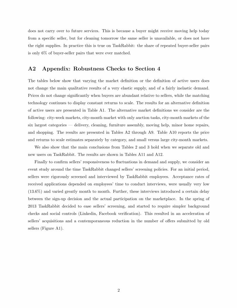
A2 Appendix: Robustness Checks to Section 4

The tables below show that varying the market definition or the definition of active users does

not change the main qualitative results of a very elastic supply, and of a fairly inelastic demand.

Prices do not change significantly when buyers are abundant relative to sellers, while the matching

technology continues to display constant returns to scale. The results for an alternative definition

of active users are presented in Table A1. The alternative market definitions we consider are the

following: city-week markets, city-month market with only auction tasks, city-month markets of the

six largest categories — delivery, cleaning, furniture assembly, moving help, minor home repairs,

and shopping. The results are presented in Tables A2 through A9. Table A10 reports the price

and returns to scale estimates separately by category, and small versus large city-month markets.

We also show that the main conclusions from Tables 2 and 3 hold when we separate old and

new users on TaskRabbit. The results are shown in Tables A11 and A12.

Finally to confirm sellers’ responsiveness to fluctuations in demand and supply, we consider an

event study around the time TaskRabbit changed sellers’ screening policies. For an initial period,

sellers were rigorously screened and interviewed by TaskRabbit employees. Acceptance rates of

received applications depended on employees’ time to conduct interviews, were usually very low

(13.6%) and varied greatly month to month. Further, these interviews introduced a certain delay

between the sign-up decision and the actual participation on the marketplace. In the spring of

2013 TaskRabbit decided to ease sellers’ screening, and started to require simpler background

checks and social controls (Linkedin, Facebook verification). This resulted in an acceleration of

sellers’ acquisitions and a contemporaneous reduction in the number of o↵ers submitted by old

sellers (Figure A1).

2

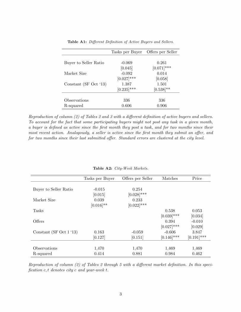
Table A1: Di↵erent Definition of Active Buyers and Sellers.

Tasks per Buyer O↵ers per Seller

Buyer to Seller Ratio -0.069 0.261[0.045] [0.071]***

Market Size -0.092 0.014[0.027]*** [0.058]

Constant (SF Oct ‘13) 1.387 1.501[0.235]*** [0.538]**

Observations 336 336R-squared 0.606 0.906

Reproduction of column (2) of Tables 2 and 3 with a di↵erent definition of active buyers and sellers.To account for the fact that some participating buyers might not post any task in a given month,a buyer is defined as active since the first month they post a task, and for two months since theirmost recent action. Analogously, a seller is active since the first month they submit an o↵er, andfor two months since their last submitted o↵er. Standard errors are clustered at the city level.

Table A2: City-Week Markets.

Tasks per Buyer O↵ers per Seller Matches Price


Market Size 0.039 0.233[0.016]** [0.022]***

Tasks 0.538 0.053[0.039]*** [0.034]

O↵ers 0.394 -0.010[0.027]*** [0.029]

Constant (SF Oct 1 ‘13) 0.163 -0.059 -0.606 3.847[0.127] [0.151] [0.146]*** [0.191]***

Observations 1,470 1,470 1,469 1,469R-squared 0.414 0.881 0.984 0.462

Reproduction of column (2) of Tables 2 through 5 with a di↵erent market definition. In this speci-fication c, t denotes city c and year-week t.

3

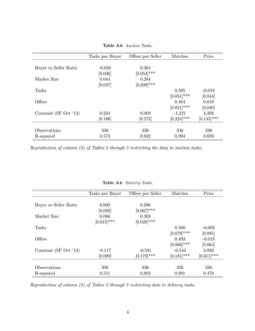
Table A3: Auction Tasks.



Market Size 0.044 0.284[0.027] [0.039]***

Tasks 0.505 -0.019[0.051]*** [0.044]

O↵ers 0.484 0.019[0.051]*** [0.040]

Constant (SF Oct ‘13) 0.234 0.003 -1.221 4.268[0.196] [0.272] [0.224]*** [0.145]***

Observations 336 336 336 336R-squared 0.573 0.932 0.994 0.693

Reproduction of column (2) of Tables 2 through 5 restricting the data to auction tasks.

Table A4: Delivery Tasks.


Buyer to Seller Ratio 0.000 0.296[0.030] [0.067]***

Market Size 0.086 0.303[0.015]*** [0.028]***

Tasks 0.500 -0.003[0.079]*** [0.085]

O↵ers 0.493 -0.019[0.066]*** [0.064]

Constant (SF Oct ‘13) -0.117 -0.591 -0.544 3.930[0.099] [0.179]*** [0.181]*** [0.311]***


Reproduction of column (2) of Tables 2 through 5 restricting data to delivery tasks.

4

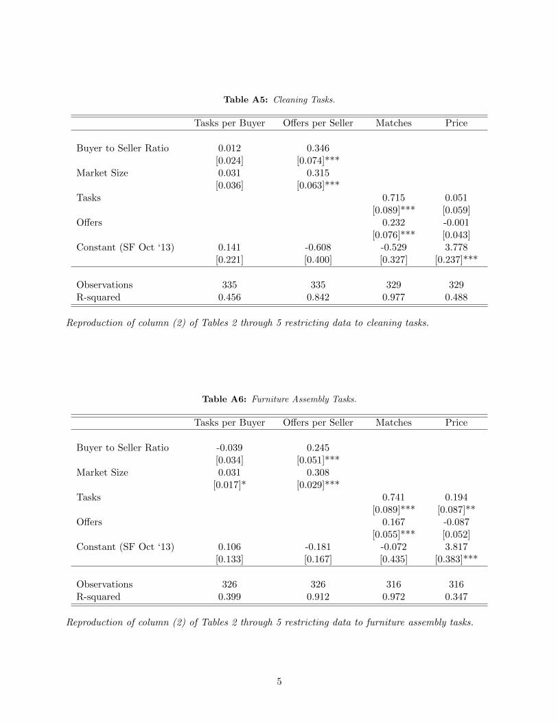
Table A5: Cleaning Tasks.



Market Size 0.031 0.315[0.036] [0.063]***

Tasks 0.715 0.051[0.089]*** [0.059]

O↵ers 0.232 -0.001[0.076]*** [0.043]

Constant (SF Oct ‘13) 0.141 -0.608 -0.529 3.778[0.221] [0.400] [0.327] [0.237]***


Reproduction of column (2) of Tables 2 through 5 restricting data to cleaning tasks.

Table A6: Furniture Assembly Tasks.



Market Size 0.031 0.308[0.017]* [0.029]***

Tasks 0.741 0.194[0.089]*** [0.087]**

O↵ers 0.167 -0.087[0.055]*** [0.052]

Constant (SF Oct ‘13) 0.106 -0.181 -0.072 3.817[0.133] [0.167] [0.435] [0.383]***


Reproduction of column (2) of Tables 2 through 5 restricting data to furniture assembly tasks.

5

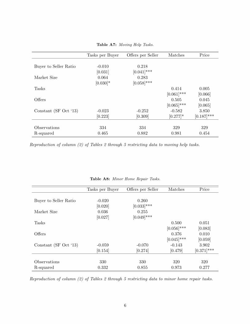
Table A7: Moving Help Tasks.



Market Size 0.064 0.283[0.030]* [0.058]***

Tasks 0.414 0.005[0.061]*** [0.066]

O↵ers 0.505 0.045[0.065]*** [0.065]

Constant (SF Oct ‘13) -0.023 -0.252 -0.582 3.850[0.223] [0.309] [0.277]* [0.187]***


Reproduction of column (2) of Tables 2 through 5 restricting data to moving help tasks.

Table A8: Minor Home Repair Tasks.



Market Size 0.036 0.255[0.027] [0.049]***

Tasks 0.500 0.051[0.056]*** [0.083]

O↵ers 0.376 0.010[0.045]*** [0.059]

Constant (SF Oct ‘13) -0.059 -0.070 -0.143 3.902[0.154] [0.274] [0.479] [0.371]***


Reproduction of column (2) of Tables 2 through 5 restricting data to minor home repair tasks.

6

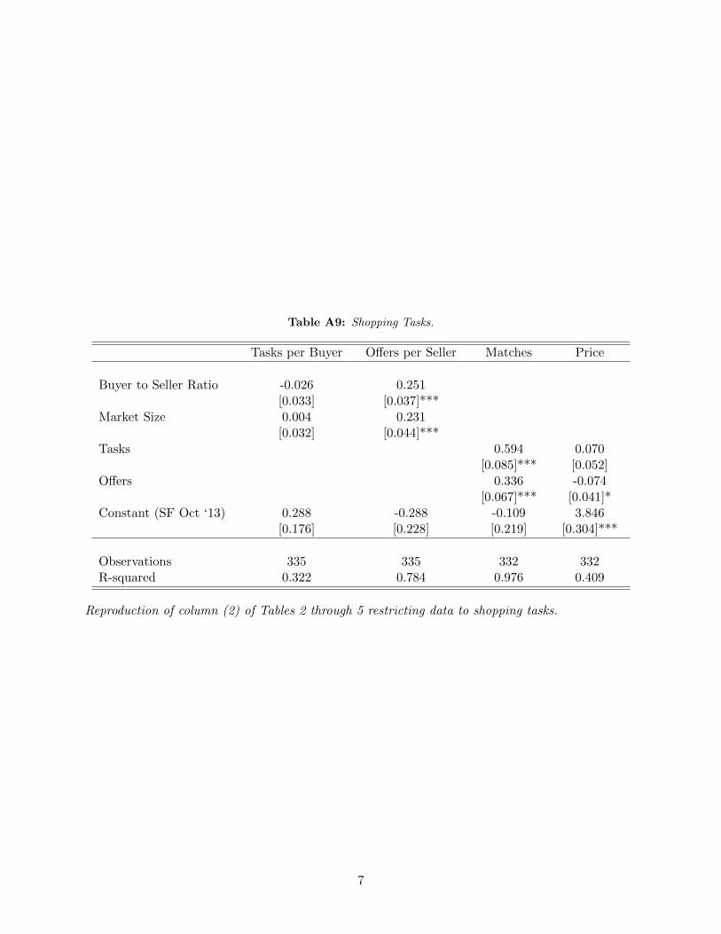
Table A9: Shopping Tasks.



Market Size 0.004 0.231[0.032] [0.044]***

Tasks 0.594 0.070[0.085]*** [0.052]

O↵ers 0.336 -0.074[0.067]*** [0.041]*

Constant (SF Oct ‘13) 0.288 -0.288 -0.109 3.846[0.176] [0.228] [0.219] [0.304]***


Reproduction of column (2) of Tables 2 through 5 restricting data to shopping tasks.

7

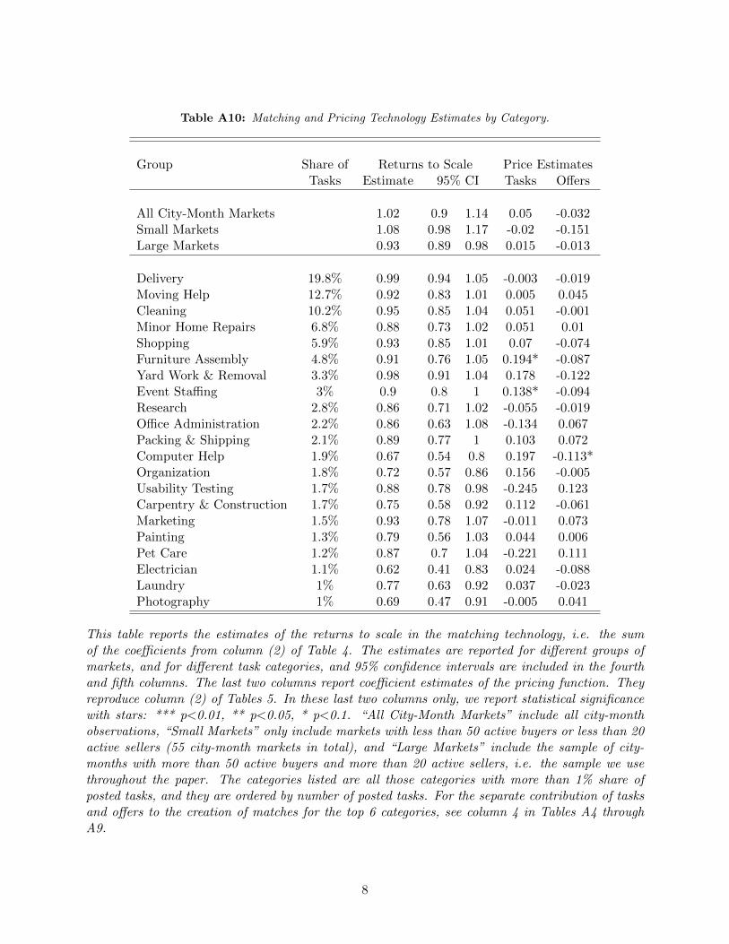
Table A10: Matching and Pricing Technology Estimates by Category.

Group Share of Returns to Scale Price EstimatesTasks Estimate 95% CI Tasks O↵ers

All City-Month Markets 1.02 0.9 1.14 0.05 -0.032Small Markets 1.08 0.98 1.17 -0.02 -0.151Large Markets 0.93 0.89 0.98 0.015 -0.013

Delivery 19.8% 0.99 0.94 1.05 -0.003 -0.019Moving Help 12.7% 0.92 0.83 1.01 0.005 0.045Cleaning 10.2% 0.95 0.85 1.04 0.051 -0.001Minor Home Repairs 6.8% 0.88 0.73 1.02 0.051 0.01Shopping 5.9% 0.93 0.85 1.01 0.07 -0.074Furniture Assembly 4.8% 0.91 0.76 1.05 0.194* -0.087Yard Work & Removal 3.3% 0.98 0.91 1.04 0.178 -0.122Event Sta�ng 3% 0.9 0.8 1 0.138* -0.094Research 2.8% 0.86 0.71 1.02 -0.055 -0.019O�ce Administration 2.2% 0.86 0.63 1.08 -0.134 0.067Packing & Shipping 2.1% 0.89 0.77 1 0.103 0.072Computer Help 1.9% 0.67 0.54 0.8 0.197 -0.113*Organization 1.8% 0.72 0.57 0.86 0.156 -0.005Usability Testing 1.7% 0.88 0.78 0.98 -0.245 0.123Carpentry & Construction 1.7% 0.75 0.58 0.92 0.112 -0.061Marketing 1.5% 0.93 0.78 1.07 -0.011 0.073Painting 1.3% 0.79 0.56 1.03 0.044 0.006Pet Care 1.2% 0.87 0.7 1.04 -0.221 0.111Electrician 1.1% 0.62 0.41 0.83 0.024 -0.088Laundry 1% 0.77 0.63 0.92 0.037 -0.023Photography 1% 0.69 0.47 0.91 -0.005 0.041

This table reports the estimates of the returns to scale in the matching technology, i.e. the sumof the coe�cients from column (2) of Table 4. The estimates are reported for di↵erent groups ofmarkets, and for di↵erent task categories, and 95% confidence intervals are included in the fourthand fifth columns. The last two columns report coe�cient estimates of the pricing function. Theyreproduce column (2) of Tables 5. In these last two columns only, we report statistical significancewith stars: *** p<0.01, ** p<0.05, * p<0.1. “All City-Month Markets” include all city-monthobservations, “Small Markets” only include markets with less than 50 active buyers or less than 20active sellers (55 city-month markets in total), and “Large Markets” include the sample of city-months with more than 50 active buyers and more than 20 active sellers, i.e. the sample we usethroughout the paper. The categories listed are all those categories with more than 1% share ofposted tasks, and they are ordered by number of posted tasks. For the separate contribution of tasksand o↵ers to the creation of matches for the top 6 categories, see column 4 in Tables A4 throughA9.

8

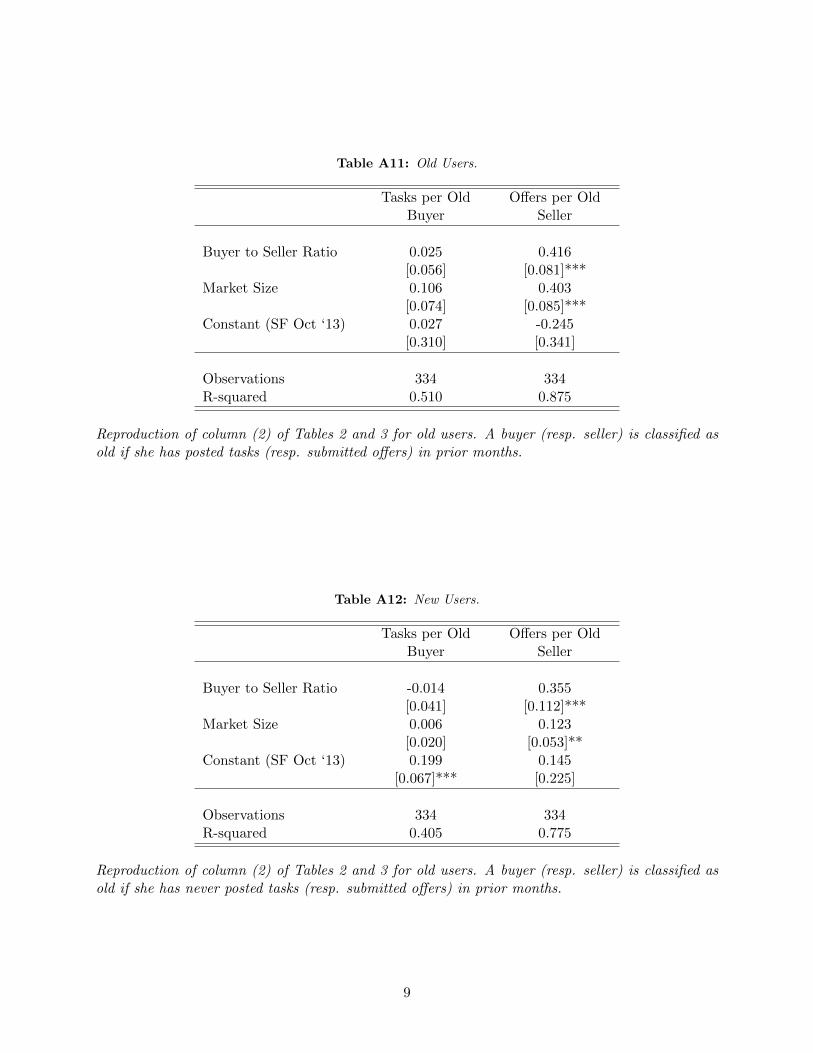
Table A11: Old Users.

Tasks per OldBuyer

O↵ers per OldSeller


Market Size 0.106 0.403[0.074] [0.085]***

Constant (SF Oct ‘13) 0.027 -0.245[0.310] [0.341]


Reproduction of column (2) of Tables 2 and 3 for old users. A buyer (resp. seller) is classified asold if she has posted tasks (resp. submitted o↵ers) in prior months.

Table A12: New Users.

Tasks per OldBuyer

O↵ers per OldSeller


Market Size 0.006 0.123[0.020] [0.053]**

Constant (SF Oct ‘13) 0.199 0.145[0.067]*** [0.225]


Reproduction of column (2) of Tables 2 and 3 for old users. A buyer (resp. seller) is classified asold if she has never posted tasks (resp. submitted o↵ers) in prior months.

9

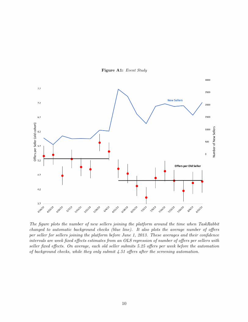
Figure A1: Event Study

The figure plots the number of new sellers joining the platform around the time when TaskRabbitchanged to automatic background checks (blue line). It also plots the average number of o↵ersper seller for sellers joining the platform before June 1, 2013. These averages and their confidenceintervals are week fixed e↵ects estimates from an OLS regression of number of o↵ers per sellers withseller fixed e↵ects. On average, each old seller submits 5.25 o↵ers per week before the automationof background checks, while they only submit 4.51 o↵ers after the screening automation.

10

A3 Appendix: Adoption

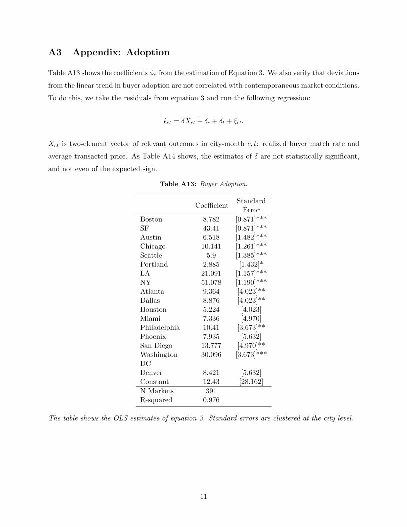
Table A13 shows the coe�cients �c from the estimation of Equation 3. We also verify that deviations

from the linear trend in buyer adoption are not correlated with contemporaneous market conditions.

To do this, we take the residuals from equation 3 and run the following regression:

✏ct = �Xct + �c + �t + ⇠ct.

Xct is two-element vector of relevant outcomes in city-month c, t: realized buyer match rate and

average transacted price. As Table A14 shows, the estimates of � are not statistically significant,

and not even of the expected sign.

Table A13: Buyer Adoption.

Coe�cientStandardError

Boston 8.782 [0.871]***SF 43.41 [0.871]***Austin 6.518 [1.482]***Chicago 10.141 [1.261]***Seattle 5.9 [1.385]***Portland 2.885 [1.432]*LA 21.091 [1.157]***NY 51.078 [1.190]***Atlanta 9.364 [4.023]**Dallas 8.876 [4.023]**Houston 5.224 [4.023]Miami 7.336 [4.970]Philadelphia 10.41 [3.673]**Phoenix 7.935 [5.632]San Diego 13.777 [4.970]**WashingtonDC

30.096 [3.673]***

Denver 8.421 [5.632]Constant 12.43 [28.162]N Markets 391R-squared 0.976

The table shows the OLS estimates of equation 3. Standard errors are clustered at the city level.

11

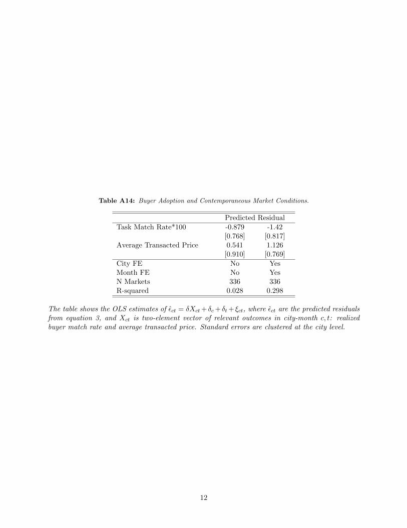
Table A14: Buyer Adoption and Contemporaneous Market Conditions.

Predicted ResidualTask Match Rate*100 -0.879 -1.42

[0.768] [0.817]Average Transacted Price 0.541 1.126

[0.910] [0.769]City FE No YesMonth FE No YesN Markets 336 336R-squared 0.028 0.298

The table shows the OLS estimates of ✏ct = �Xct+ �c+ �t+ ⇠ct, where ✏ct are the predicted residualsfrom equation 3, and Xct is two-element vector of relevant outcomes in city-month c, t: realizedbuyer match rate and average transacted price. Standard errors are clustered at the city level.

12

A4 Appendix: Retention

To support our main identification assumption, we verify that, conditional on the outcomes (matches

and prices) in a current market, expectations on future outcomes do not a↵ect the propensity to

stay or leave the marketplace. To do this we run OLS regressions similar to equation 4:

log

✓stayct

1� stayct

◆= ✓0Xct + ✓1Xt+1,c + ✓2Xt+2,c + ✓3Xt+3,c + ✓t + ✓c + ✏ct ,

Xct is defined as in equation 4. The regression is run separately for buyers and sellers, so the

match rate for buyers is the task success probability, while the match rate for sellers is the o↵er

acceptance rate. The 6-element vector (Xt+1,c, Xt+2,c, Xt+3,c) contains the realized match rates and

prices in the following three months within the same city. If users did not base their decision to

stay or leave the marketplace on expectations of future outcomes we would expect the 6-element

coe�cient vector (✓1, ✓2, ✓3) to be non significant, both for buyers and for sellers.

Results are presented in Tables A15 (for buyers) and A16 (for sellers). Each table has four

columns, corresponding to four di↵erent specifications. The first specification estimates ✓0 without

including forward variables – this is precisely Equation 4 from Section 5. Each other specification

sequentially adds the outcomes of the following month, two-months ahead, and three-months ahead.

The final column is the full specification. With the exception of just one coe�cient in the buyers’

regression (the coe�cient on the three-month-ahead transacted price), all other coe�cients from

(✓1, ✓2, ✓3) are not statistically di↵erent from zero, and in some cases even have the opposite sign.

Despite the small number of observations, another important observation from the two tables is that

users appear to base their decisions to stay on the marketplace particularly on the contemporaneous

match rate. Adding forward variables does not change the e↵ect of match rate much nor helps

improve the goodness of fit of the estimation.

13

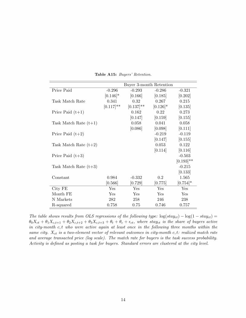
Table A15: Buyers’ Retention.

Buyer 3-month RetentionPrice Paid -0.296 -0.293 -0.286 -0.321

[0.146]* [0.166] [0.185] [0.202]Task Match Rate 0.341 0.32 0.267 0.215

[0.117]** [0.137]** [0.126]* [0.135]Price Paid (t+1) 0.162 0.22 0.273

[0.147] [0.159] [0.155]Task Match Rate (t+1) 0.058 0.041 0.058

[0.086] [0.098] [0.111]Price Paid (t+2) -0.219 -0.119

[0.147] [0.155]Task Match Rate (t+2) 0.053 0.122

[0.114] [0.116]Price Paid (t+3) -0.503

[0.193]**Task Match Rate (t+3) -0.215

[0.133]Constant 0.984 -0.332 0.2 1.565

[0.566] [0.729] [0.775] [0.754]*City FE Yes Yes Yes YesMonth FE Yes Yes Yes YesN Markets 282 258 246 238R-squared 0.758 0.75 0.746 0.757

The table shows results from OLS regressions of the following type: log(stayct)� log(1� stayct) =✓0Xct + ✓1Xc,t+1 + ✓2Xc,t+2 + ✓3Xc,t+3 + ✓t + ✓c + ✏ct, where stayct is the share of buyers activein city-month c, t who were active again at least once in the following three months within thesame city. Xct is a two-element vector of relevant outcomes in city-month c, t: realized match rateand average transacted price (log scale). The match rate for buyers is the task success probability.Activity is defined as posting a task for buyers. Standard errors are clustered at the city level.

14

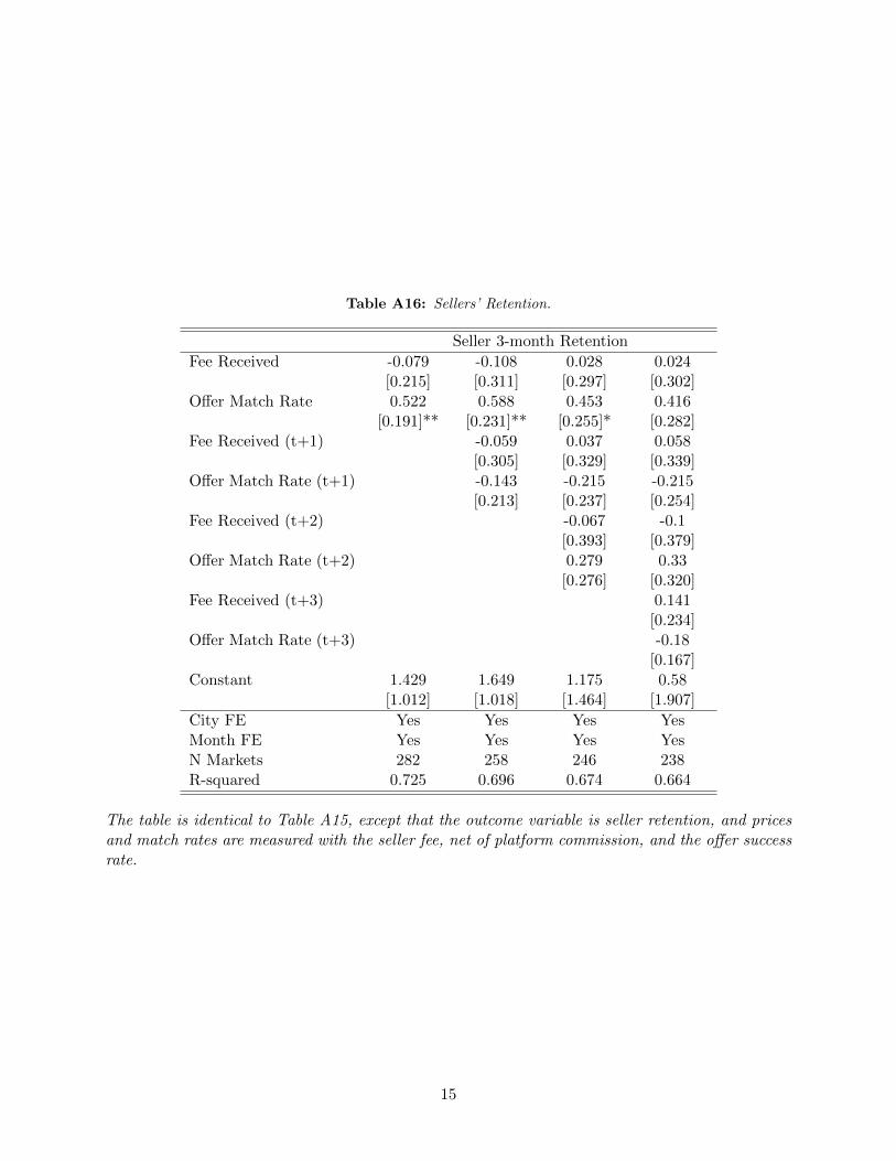
Table A16: Sellers’ Retention.

Seller 3-month RetentionFee Received -0.079 -0.108 0.028 0.024

[0.215] [0.311] [0.297] [0.302]O↵er Match Rate 0.522 0.588 0.453 0.416

[0.191]** [0.231]** [0.255]* [0.282]Fee Received (t+1) -0.059 0.037 0.058

[0.305] [0.329] [0.339]O↵er Match Rate (t+1) -0.143 -0.215 -0.215

[0.213] [0.237] [0.254]Fee Received (t+2) -0.067 -0.1

[0.393] [0.379]O↵er Match Rate (t+2) 0.279 0.33

[0.276] [0.320]Fee Received (t+3) 0.141

[0.234]O↵er Match Rate (t+3) -0.18

[0.167]Constant 1.429 1.649 1.175 0.58

[1.012] [1.018] [1.464] [1.907]City FE Yes Yes Yes YesMonth FE Yes Yes Yes YesN Markets 282 258 246 238R-squared 0.725 0.696 0.674 0.664

The table is identical to Table A15, except that the outcome variable is seller retention, and pricesand match rates are measured with the seller fee, net of platform commission, and the o↵er successrate.

15

A5 Appendix: Estimates of the Pricing and Matching Functions

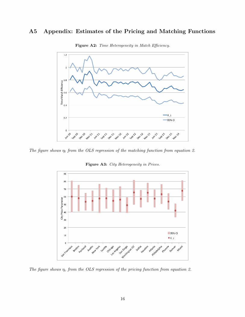
Figure A2: Time Heterogeneity in Match E�ciency.

The figure shows ⌘t from the OLS regression of the matching function from equation 2.

Figure A3: City Heterogeneity in Prices.

The figure shows ⌘c from the OLS regression of the pricing function from equation 2.

16

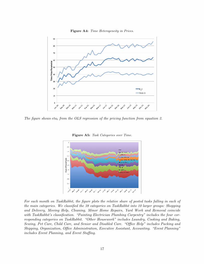
Figure A4: Time Heterogeneity in Prices.

The figure shows etat from the OLS regression of the pricing function from equation 2.

Figure A5: Task Categories over Time.

For each month on TaskRabbit, the figure plots the relative share of posted tasks falling in each ofthe main categories. We classified the 38 categories on TaskRabbit into 10 larger groups: Shoppingand Delivery, Moving Help, Cleaning, Minor Home Repairs, Yard Work and Removal coincidewith TaskRabbit’s classification. “Painting Electrician Plumbing Carpentry” includes the four cor-responding categories on TaskRabbit. “Other Housework” includes Laundry, Cooking and Baking,Sewing, Pet Care, Child Care, and Senior and Disabled Care. “O�ce Help” includes Packing andShipping, Organization, O�ce Administration, Executive Assistant, Accounting. “Event Planning”includes Event Planning, and Event Sta�ng.

17

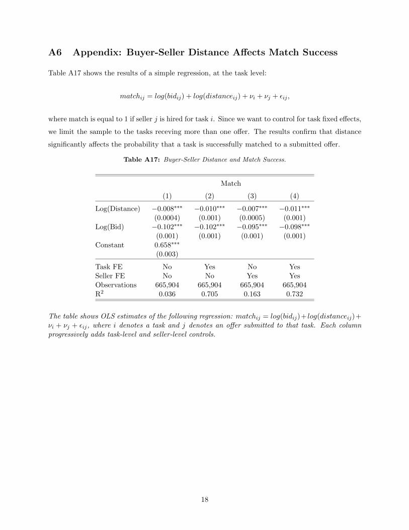
A6 Appendix: Buyer-Seller Distance A↵ects Match Success

Table A17 shows the results of a simple regression, at the task level:

matchij = log(bidij) + log(distanceij) + ⌫i + ⌫j + ✏ij ,

where match is equal to 1 if seller j is hired for task i. Since we want to control for task fixed e↵ects,

we limit the sample to the tasks receving more than one o↵er. The results confirm that distance

significantly a↵ects the probability that a task is successfully matched to a submitted o↵er.

Table A17: Buyer-Seller Distance and Match Success.

Match

(1) (2) (3) (4)

Log(Distance) �0.008⇤⇤⇤ �0.010⇤⇤⇤ �0.007⇤⇤⇤ �0.011⇤⇤⇤

(0.0004) (0.001) (0.0005) (0.001)Log(Bid) �0.102⇤⇤⇤ �0.102⇤⇤⇤ �0.095⇤⇤⇤ �0.098⇤⇤⇤

(0.001) (0.001) (0.001) (0.001)Constant 0.658⇤⇤⇤

(0.003)

Task FE No Yes No YesSeller FE No No Yes YesObservations 665,904 665,904 665,904 665,904R2 0.036 0.705 0.163 0.732

The table shows OLS estimates of the following regression: matchij = log(bidij)+ log(distanceij)+⌫i + ⌫j + ✏ij, where i denotes a task and j denotes an o↵er submitted to that task. Each columnprogressively adds task-level and seller-level controls.

18

Documents

APPENDIX Outsourcing Tasks Online: Matching Supply … · APPENDIX Outsourcing Tasks Online: Matching Supply and Demand on Peer-to-Peer Internet Platforms Zo¨e Cullen and Chiara