APPENDIX Outsourcing Tasks Online: Matching Supply and

APPENDIX

Outsourcing Tasks Online:

Matching Supply and Demand on Peer-to-Peer Internet Platforms

Zoe Cullen and Chiara Farronato

A1 Appendix: Additional Tables and Figures

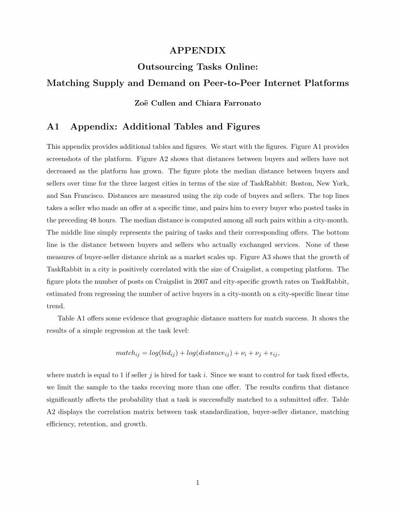
This appendix provides additional tables and figures. We start with the figures. Figure A1 provides

screenshots of the platform. Figure A2 shows that distances between buyers and sellers have not

decreased as the platform has grown. The figure plots the median distance between buyers and

sellers over time for the three largest cities in terms of the size of TaskRabbit: Boston, New York,

and San Francisco. Distances are measured using the zip code of buyers and sellers. The top lines

takes a seller who made an o↵er at a specific time, and pairs him to every buyer who posted tasks in

the preceding 48 hours. The median distance is computed among all such pairs within a city-month.

The middle line simply represents the pairing of tasks and their corresponding o↵ers. The bottom

line is the distance between buyers and sellers who actually exchanged services. None of these

measures of buyer-seller distance shrink as a market scales up. Figure A3 shows that the growth of

TaskRabbit in a city is positively correlated with the size of Craigslist, a competing platform. The

figure plots the number of posts on Craigslist in 2007 and city-specific growth rates on TaskRabbit,

estimated from regressing the number of active buyers in a city-month on a city-specific linear time

trend.

Table A1 o↵ers some evidence that geographic distance matters for match success. It shows the

results of a simple regression at the task level:

matchij = log(bidij) + log(distanceij) + ⌫i + ⌫j + ✏ij ,

where match is equal to 1 if seller j is hired for task i. Since we want to control for task fixed e↵ects,

we limit the sample to the tasks receving more than one o↵er. The results confirm that distance

significantly a↵ects the probability that a task is successfully matched to a submitted o↵er. Table

A2 displays the correlation matrix between task standardization, buyer-seller distance, matching

e�ciency, retention, and growth.

1

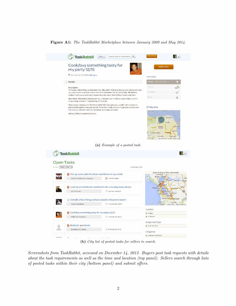
Figure A1: The TaskRabbit Marketplace between January 2009 and May 2014.

(a) Example of a posted task.

(b) City list of posted tasks for sellers to search.

Screenshots from TaskRabbit, accessed on December 14, 2013. Buyers post task requests with detailsabout the task requirements as well as the time and location (top panel). Sellers search through listsof posted tasks within their city (bottom panel) and submit o↵ers.

2

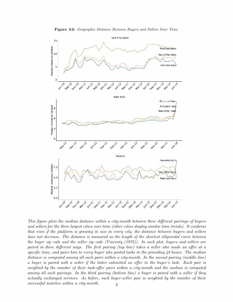
Figure A2: Geographic Distance Between Buyers and Sellers Over Time.

This figure plots the median distance within a city-month between three di↵erent pairings of buyersand sellers for the three largest cities over time (other cities display similar time trends). It confirmsthat even if the platform is growing in size in every city, the distance between buyers and sellersdoes not decrease. The distance is measured as the length of the shortest ellipsoidal curve betweenthe buyer zip code and the seller zip code (Vincenty (1975)). In each plot, buyers and sellers arepaired in three di↵erent ways. The first pairing (top line) takes a seller who made an o↵er at aspecific time, and pairs him to every buyer who posted tasks in the preceding 48 hours. The mediandistance is computed among all such pairs within a city-month. In the second pairing (middle line)a buyer is paired with a seller if the latter submitted an o↵er to the buyer’s task. Each pair isweighted by the number of their task-o↵er pairs within a city-month and the median is computedamong all such pairings. In the third pairing (bottom line) a buyer is paired with a seller if theyactually exchanged services. As before, each buyer-seller pair is weighted by the number of theirsuccessful matches within a city-month. 3

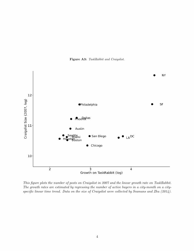
Figure A3: TaskRabbit and Craigslist.

This figure plots the number of posts on Craigslist in 2007 and the linear growth rate on TaskRabbit.The growth rates are estimated by regressing the number of active buyers in a city-month on a city-specific linear time trend. Data on the size of Craigslist were collected by Seamans and Zhu (2014).

4

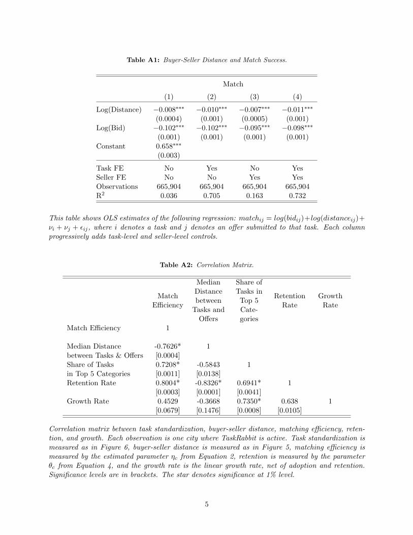
Table A1: Buyer-Seller Distance and Match Success.

Match

(1) (2) (3) (4)

Log(Distance) �0.008⇤⇤⇤ �0.010⇤⇤⇤ �0.007⇤⇤⇤ �0.011⇤⇤⇤

(0.0004) (0.001) (0.0005) (0.001)Log(Bid) �0.102⇤⇤⇤ �0.102⇤⇤⇤ �0.095⇤⇤⇤ �0.098⇤⇤⇤

(0.001) (0.001) (0.001) (0.001)Constant 0.658⇤⇤⇤

(0.003)

Task FE No Yes No YesSeller FE No No Yes YesObservations 665,904 665,904 665,904 665,904R2 0.036 0.705 0.163 0.732

This table shows OLS estimates of the following regression: matchij = log(bidij)+log(distanceij)+⌫i + ⌫j + ✏ij, where i denotes a task and j denotes an o↵er submitted to that task. Each columnprogressively adds task-level and seller-level controls.

Table A2: Correlation Matrix.

MatchE�ciency

MedianDistancebetweenTasks andO↵ers

Share ofTasks inTop 5Cate-gories

RetentionRate

GrowthRate

Match E�ciency 1

Median Distance -0.7626* 1between Tasks & O↵ers [0.0004]Share of Tasks 0.7208* -0.5843 1in Top 5 Categories [0.0011] [0.0138]Retention Rate 0.8004* -0.8326* 0.6941* 1

[0.0003] [0.0001] [0.0041]Growth Rate 0.4529 -0.3668 0.7350* 0.638 1

[0.0679] [0.1476] [0.0008] [0.0105]

Correlation matrix between task standardization, buyer-seller distance, matching e�ciency, reten-tion, and growth. Each observation is one city where TaskRabbit is active. Task standardization ismeasured as in Figure 6, buyer-seller distance is measured as in Figure 5, matching e�ciency ismeasured by the estimated parameter ⌘c from Equation 2, retention is measured by the parameter✓c from Equation 4, and the growth rate is the linear growth rate, net of adoption and retention.Significance levels are in brackets. The star denotes significance at 1% level.

5

A2 Appendix: Robustness Checks to Section 4

This appendix discusses our market definition, and provides a number of robustness checks to the

results presented in Section 4.

In Section 4 we define a market at the city-month level, and assume homogeneity among buyers

posting tasks and sellers submitting o↵ers. This definition is motivated by several considerations.

First, we do not separate markets along task categories - cleaning, furniture assembly, and so on -

because sellers do not specialize. Of the sellers who submitted 10 o↵ers or more, 63.6% did so in

more than 10 categories, and of the sellers who were successfully matched to more than 10 tasks,

43% performed tasks in more than 10 categories. Second, we follow TaskRabbit’s business practice

and do not separate markets into geographic partitions smaller than the metropolitan boundaries.34

Third, we choose calendar months as the relevant time window in order to balance the short time

period in which tasks receive o↵ers with the need for there to be enough activity in each market to

estimate match probabilities, average prices, and search and posting intensities.

Homogeneity of tasks seems reasonable because so many of the tasks are relatively standard

and do not require specialized skills, and most sellers send o↵ers to tasks belonging to multiple

categories. However, considering task heterogeneity explicitly allows us to gain a more nuanced

view of search frictions, as we show in Section 5. The homogeneity of buyers and sellers implies

that all buyers choose the same task posting strategy and all sellers choose the same level of search

intensity. Homogeneity of buyers is less of a concern given that they tend to post a small number

of tasks and their repeated use of the marketplace is limited. Sellers, on the other hand, can build

their experience and reputation on the marketplace.

The homogeneity assumptions allow us to limit the choices available to buyers and sellers to

solely posting tasks and submitting o↵ers. We do not explicitly model the selection of tasks to which

a seller makes o↵ers, nor a buyer’s choice to assign the task to a specific bidder. We assume that the

number of matches formed between buyers and sellers of services, as well as the price at which they

trade, are determined by a matching and a pricing function. The underlying frictions from actual

task heterogeneity and information asymmetries are not made explicit, but summarized in a match

productivity parameter. In this sense, the paper complements work by Fradkin (2019) on search

ine�ciencies on Airbnb, and Horton (2019) on congestion on Upwork. These papers study their

respective peer-to-peer markets and quantify the e�ciency losses due to specific types of friction

that an improved marketplace design can help alleviate. Our approach takes the “natural” level

of frictions on the marketplace as given and shows that the latter does not change considerably as

34We do not observe any sort of clear neighborhood partitioning in the data, although the setup on TaskRabbitdoes not preclude it.

6

more or fewer buyers, both in absolute and relative terms, are present in the market.

Our framework also assumes that services are independent of each other, both within a market

and across markets. This implies that there are no externalities to other services from completing

one task with a specific partner. Most buyers only post one task in a city-month, which helps justify

this assumption. Moreover, matches in one market have no externalities on future matches. This

e↵ectively assumes that the benefit of trading one service with a specific partner does not carry

over to future services. This is because a buyer might receive moving help today from a specific

seller, but that same seller may be unavailable for cleaning tomorrow, or might not have the right

supplies. This does occur on TaskRabbit: the share of repeat buyer-seller pairs is only 6% of all

pairs ever matched.

This appendix also o↵ers robustness checks to the results in Section 4. Our results do not

change when we segment the data into finer markets with respect to time and service categories,

or when we account for some degree of buyer and seller heterogeneity.

First, since we only observe task posting and o↵er submission, we cannot distinguish between

buyers and sellers who chose not to post a task or submit an o↵er because of unfavorable market

conditions, and those who were completely disengaged from TaskRabbit. If there were no hetero-

geneity across buyers, then the number of buyers posting tasks would match the number of buyers

participating on the platform. In practice that is not true: individual buyers request di↵erent

numbers of tasks. A participating buyer might be more likely to post a request in a market where

buyers are scarce relative to sellers than in a market where buyers are abundant. To account for

this, we consider a buyer to be active beginning with the first month they post a task and for two

months following their most recent action. We do the same for sellers. We re-estimate Equation 1,

where the number of active buyers and sellers, as well as the number of tasks per buyer and o↵ers

per seller, are adjusted accordingly. The estimates in Table A4 confirm our main results.

Second, we show that sellers decreased their e↵orts in response to a change in TaskRabbit’s

screening policies, which increased the number of new sellers joining the platform. In the spring of

2013, TaskRabbit decided to ease their screening policies for sellers and started to require simpler

background checks and social controls (automatic LinkedIn and Facebook verification). This re-

sulted in an acceleration in the acquisition of sellers. In Figure A4, we use an event study approach

to show that older providers sharply decreased the number of o↵ers they submitted immediately

following the change in new seller screening.

Third, we confirm that our results remain unchanged if we focus on auction tasks only, if we

restrict attention to individual service categories, and if we consider city-weeks as the relevant

market. We consider the following alternative market definitions: city-week markets, city-month

7

markets with only auction tasks, and city-month markets of the six largest categories—delivery,

cleaning, furniture assembly, moving help, minor home repairs, and shopping. The results are

presented in Tables A5 through A12. Table A13 reports the price and returns to scale estimates

separately by category, and small versus large city-month markets.

Fourth, we show that the main conclusions hold when we account for some degree of user

heterogeneity. Specifically, we separate old and new users on TaskRabbit. The results are shown

in Tables A14 and A15.

Fifth, to control for the fact that platform growth in one month may depend on previous growth,

we run panel data regressions with the one-month lag of active buyers and sellers as additional

controls, which does not change our results (Table A16). Note that this exercise also addresses the

concern that media articles may be caused by, rather than be the cause of, platform growth. Using

the one-month lag partially addresses the concern of reverse causality, but it is still possible that

high platform growth in the previous month leads to both an increase in media articles in that

month and an increase in adoption the present month. The panel data regressions with the lag of

our explanatory variables of interest as additional controls addresses this concern.

Sixth, we rerun the regressions from Table 5 using the number of buyers and the number of

sellers as dependent variables. Table A17 confirms the absence of economies of scale in matching,

i.e., we cannot reject the null that doubling buyers and sellers only doubles the number of matches.

Finally, to check whether entrants are systematically di↵erent in markets with a higher number

of participants, we run robustness regressions of the following type:

matchrct = ↵1 log (Bct) + ↵2 log (Sct) + ↵3firstrct

+ ↵4firstrct ⇤ log (Bct) + ↵5firstrct ⇤ log (Sct) + ⌘c + ⌘t + ✏rct

We run these regressions for requests and o↵ers separately, and the outcome variable is equal to

one if the request or o↵er is successful. Thus, for requests, r denotes a request posted in market c, t,

and firstrct is equal to 1 if the request was posted on the very first day the buyer posted requests.

For o↵ers, r denotes the o↵er submitted, and firstrct is equal to 1 if the o↵er was submitted on

the very first day the seller submitted o↵ers. The estimate of interest is ↵4 + ↵5. If the sum of

the two coe�cients is negative, it would imply a negative selection for o↵ers and requests when

markets are larger. The results are presented in Table A18. We cannot reject the hypothesis that

the sum of the two coe�cients is zero in either column at any conventional significance level. This

result supports the hypothesis that entrants in large markets are not systematically di↵erent from

entrants in small markets.

8

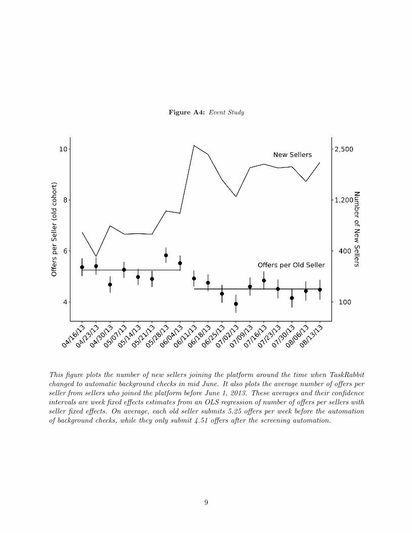
Figure A4: Event Study

This figure plots the number of new sellers joining the platform around the time when TaskRabbitchanged to automatic background checks in mid June. It also plots the average number of o↵ers perseller from sellers who joined the platform before June 1, 2013. These averages and their confidenceintervals are week fixed e↵ects estimates from an OLS regression of number of o↵ers per sellers withseller fixed e↵ects. On average, each old seller submits 5.25 o↵ers per week before the automationof background checks, while they only submit 4.51 o↵ers after the screening automation.

9

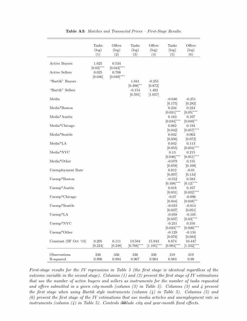
Table A3: Matches and Transacted Prices – First-Stage Results.

Tasks(log)

O↵ers(log)

Tasks(log)

O↵ers(log)

Tasks(log)

O↵ers(log)

(1) (2) (3) (4) (5) (6)

Active Buyers 1.025 0.534[0.03]⇤⇤⇤ [0.043]⇤⇤⇤

Active Sellers 0.025 0.708[0.036] [0.049]⇤⇤⇤

“Bartik” Buyers 1.041 -0.255[0.498]⇤⇤ [0.872]

“Bartik” Sellers -0.154 1.482[0.591] [1.057]

Media -0.046 -0.251[0.175] [0.282]

Media*Boston 0.234 0.224[0.031]⇤⇤⇤ [0.05]⇤⇤⇤

Media*Austin 0.163 0.107[0.034]⇤⇤⇤ [0.049]⇤⇤

Media*Chicago 0.062 0.194[0.042] [0.057]⇤⇤⇤

Media*Seattle 0.042 0.062[0.056] [0.072]

Media*LA 0.042 0.113[0.055] [0.034]⇤⇤⇤

Media*NYC 0.13 0.215[0.046]⇤⇤⇤ [0.051]⇤⇤⇤

Media*Other -0.079 0.155[0.058] [0.108]

Unemployment Rate 0.012 -0.01[0.097] [0.134]

Unemp*Boston -0.552 0.583[0.108]⇤⇤⇤ [0.12]⇤⇤⇤

Unemp*Austin 0.018 0.167[0.031] [0.032]⇤⇤⇤

Unemp*Chicago -0.07 -0.096[0.044] [0.048]⇤⇤

Unemp*Seattle -0.033 -0.014[0.037] [0.051]

Unemp*LA -0.058 -0.105[0.037] [0.03]⇤⇤⇤

Unemp*NYC -0.251 0.316[0.023]⇤⇤⇤ [0.026]⇤⇤⇤

Unemp*Other -0.128 -0.134[0.076] [0.083]

Constant (SF Oct ‘13) 0.205 0.111 13.584 15.943 8.874 10.447[0.224] [0.248] [0.766]⇤⇤⇤ [1.105]⇤⇤⇤ [0.904]⇤⇤⇤ [1.332]⇤⇤⇤

Observations 336 336 336 336 319 319R-squared 0.996 0.994 0.967 0.964 0.983 0.98

First-stage results for the IV regressions in Table 5 (the first stage is identical regardless of theoutcome variable in the second stage). Columns (1) and (2) present the first stage of IV estimationsthat use the number of active buyers and sellers as instruments for the number of tasks requestedand o↵ers submitted in a given city-month (column (3) in Table 5). Columns (3) and 4 presentthe first stage when using Bartik style instruments (column (4) in Table 5). Columns (5) and(6) present the first stage of the IV estimations that use media articles and unemployment rate asinstruments (column (4) in Table 5). Controls include city and year-month fixed e↵ects.10

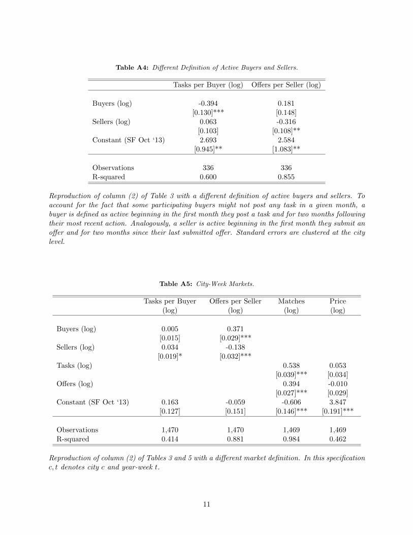
Table A4: Di↵erent Definition of Active Buyers and Sellers.

Tasks per Buyer (log) O↵ers per Seller (log)

Buyers (log) -0.394 0.181[0.130]*** [0.148]

Sellers (log) 0.063 -0.316[0.103] [0.108]**

Constant (SF Oct ‘13) 2.693 2.584[0.945]** [1.083]**

Observations 336 336R-squared 0.600 0.855

Reproduction of column (2) of Table 3 with a di↵erent definition of active buyers and sellers. Toaccount for the fact that some participating buyers might not post any task in a given month, abuyer is defined as active beginning in the first month they post a task and for two months followingtheir most recent action. Analogously, a seller is active beginning in the first month they submit ano↵er and for two months since their last submitted o↵er. Standard errors are clustered at the citylevel.

Table A5: City-Week Markets.

Tasks per Buyer(log)

O↵ers per Seller(log)

Matches(log)

Price(log)

Buyers (log) 0.005 0.371[0.015] [0.029]***

Sellers (log) 0.034 -0.138[0.019]* [0.032]***

Tasks (log) 0.538 0.053[0.039]*** [0.034]

O↵ers (log) 0.394 -0.010[0.027]*** [0.029]

Constant (SF Oct ‘13) 0.163 -0.059 -0.606 3.847[0.127] [0.151] [0.146]*** [0.191]***

Observations 1,470 1,470 1,469 1,469R-squared 0.414 0.881 0.984 0.462

Reproduction of column (2) of Tables 3 and 5 with a di↵erent market definition. In this specificationc, t denotes city c and year-week t.

11

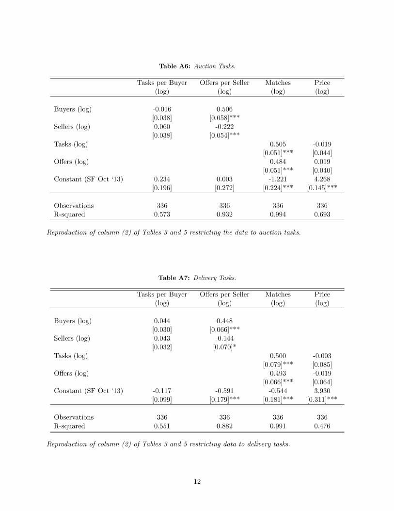
Table A6: Auction Tasks.



Matches(log)

Price(log)

Buyers (log) -0.016 0.506[0.038] [0.058]***

Sellers (log) 0.060 -0.222[0.038] [0.054]***

Tasks (log) 0.505 -0.019[0.051]*** [0.044]

O↵ers (log) 0.484 0.019[0.051]*** [0.040]

Constant (SF Oct ‘13) 0.234 0.003 -1.221 4.268[0.196] [0.272] [0.224]*** [0.145]***

Observations 336 336 336 336R-squared 0.573 0.932 0.994 0.693

Reproduction of column (2) of Tables 3 and 5 restricting the data to auction tasks.

Table A7: Delivery Tasks.



Matches(log)

Price(log)

Buyers (log) 0.044 0.448[0.030] [0.066]***

Sellers (log) 0.043 -0.144[0.032] [0.070]*

Tasks (log) 0.500 -0.003[0.079]*** [0.085]

O↵ers (log) 0.493 -0.019[0.066]*** [0.064]

Constant (SF Oct ‘13) -0.117 -0.591 -0.544 3.930[0.099] [0.179]*** [0.181]*** [0.311]***


Reproduction of column (2) of Tables 3 and 5 restricting data to delivery tasks.

12

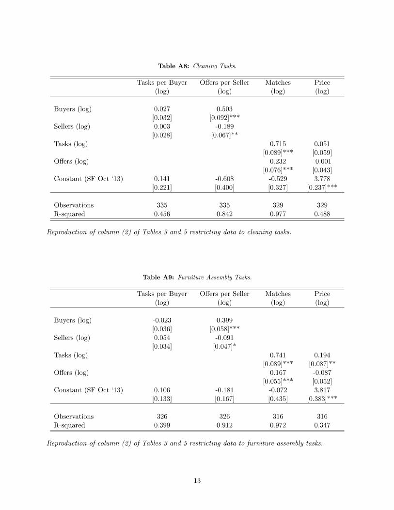
Table A8: Cleaning Tasks.



Matches(log)

Price(log)

Buyers (log) 0.027 0.503[0.032] [0.092]***

Sellers (log) 0.003 -0.189[0.028] [0.067]**

Tasks (log) 0.715 0.051[0.089]*** [0.059]

O↵ers (log) 0.232 -0.001[0.076]*** [0.043]

Constant (SF Oct ‘13) 0.141 -0.608 -0.529 3.778[0.221] [0.400] [0.327] [0.237]***


Reproduction of column (2) of Tables 3 and 5 restricting data to cleaning tasks.

Table A9: Furniture Assembly Tasks.



Matches(log)

Price(log)

Buyers (log) -0.023 0.399[0.036] [0.058]***

Sellers (log) 0.054 -0.091[0.034] [0.047]*

Tasks (log) 0.741 0.194[0.089]*** [0.087]**

O↵ers (log) 0.167 -0.087[0.055]*** [0.052]

Constant (SF Oct ‘13) 0.106 -0.181 -0.072 3.817[0.133] [0.167] [0.435] [0.383]***


Reproduction of column (2) of Tables 3 and 5 restricting data to furniture assembly tasks.

13

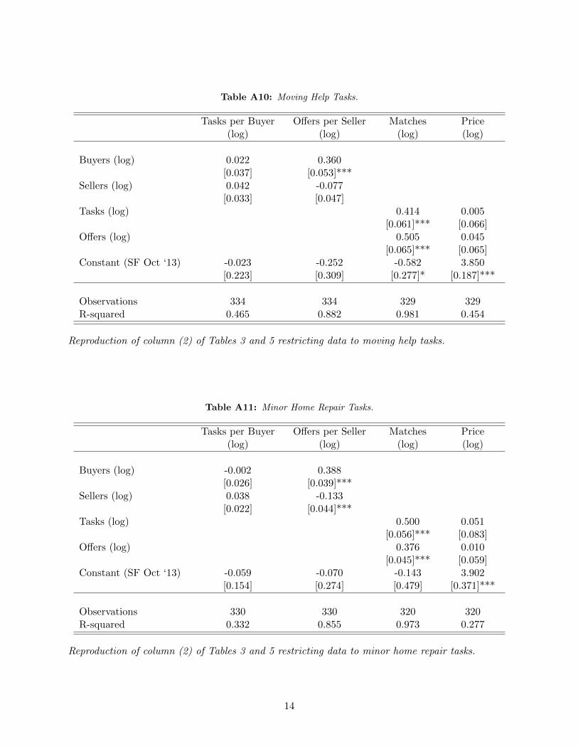
Table A10: Moving Help Tasks.



Matches(log)

Price(log)

Buyers (log) 0.022 0.360[0.037] [0.053]***

Sellers (log) 0.042 -0.077[0.033] [0.047]

Tasks (log) 0.414 0.005[0.061]*** [0.066]

O↵ers (log) 0.505 0.045[0.065]*** [0.065]

Constant (SF Oct ‘13) -0.023 -0.252 -0.582 3.850[0.223] [0.309] [0.277]* [0.187]***


Reproduction of column (2) of Tables 3 and 5 restricting data to moving help tasks.

Table A11: Minor Home Repair Tasks.



Matches(log)

Price(log)

Buyers (log) -0.002 0.388[0.026] [0.039]***

Sellers (log) 0.038 -0.133[0.022] [0.044]***

Tasks (log) 0.500 0.051[0.056]*** [0.083]

O↵ers (log) 0.376 0.010[0.045]*** [0.059]

Constant (SF Oct ‘13) -0.059 -0.070 -0.143 3.902[0.154] [0.274] [0.479] [0.371]***


Reproduction of column (2) of Tables 3 and 5 restricting data to minor home repair tasks.

14

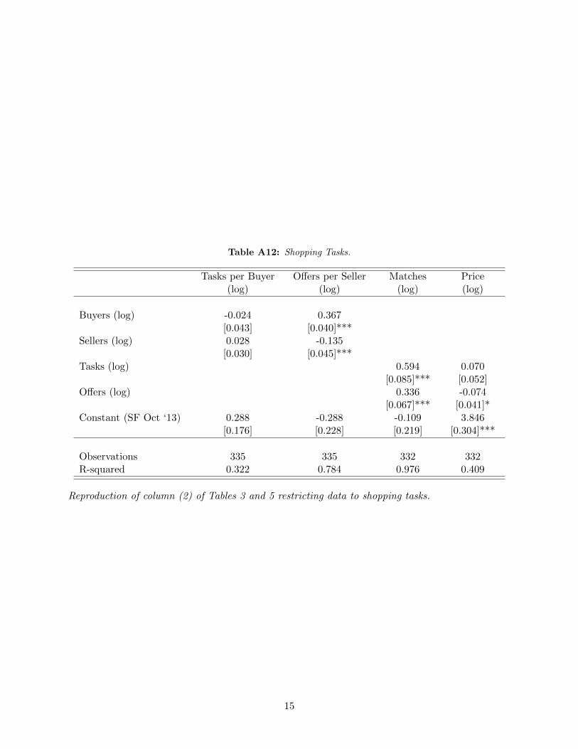
Table A12: Shopping Tasks.



Matches(log)

Price(log)

Buyers (log) -0.024 0.367[0.043] [0.040]***

Sellers (log) 0.028 -0.135[0.030] [0.045]***

Tasks (log) 0.594 0.070[0.085]*** [0.052]

O↵ers (log) 0.336 -0.074[0.067]*** [0.041]*

Constant (SF Oct ‘13) 0.288 -0.288 -0.109 3.846[0.176] [0.228] [0.219] [0.304]***


Reproduction of column (2) of Tables 3 and 5 restricting data to shopping tasks.

15

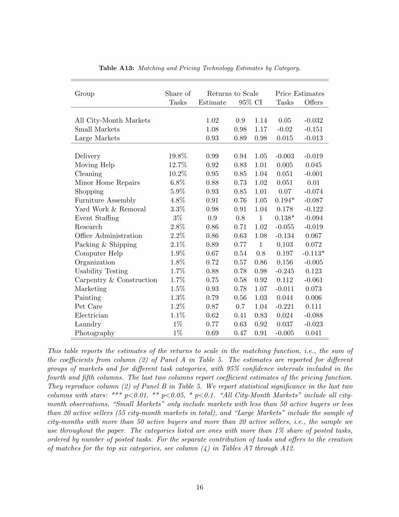
Table A13: Matching and Pricing Technology Estimates by Category.

Group Share of Returns to Scale Price EstimatesTasks Estimate 95% CI Tasks O↵ers

All City-Month Markets 1.02 0.9 1.14 0.05 -0.032Small Markets 1.08 0.98 1.17 -0.02 -0.151Large Markets 0.93 0.89 0.98 0.015 -0.013

Delivery 19.8% 0.99 0.94 1.05 -0.003 -0.019Moving Help 12.7% 0.92 0.83 1.01 0.005 0.045Cleaning 10.2% 0.95 0.85 1.04 0.051 -0.001Minor Home Repairs 6.8% 0.88 0.73 1.02 0.051 0.01Shopping 5.9% 0.93 0.85 1.01 0.07 -0.074Furniture Assembly 4.8% 0.91 0.76 1.05 0.194* -0.087Yard Work & Removal 3.3% 0.98 0.91 1.04 0.178 -0.122Event Sta�ng 3% 0.9 0.8 1 0.138* -0.094Research 2.8% 0.86 0.71 1.02 -0.055 -0.019O�ce Administration 2.2% 0.86 0.63 1.08 -0.134 0.067Packing & Shipping 2.1% 0.89 0.77 1 0.103 0.072Computer Help 1.9% 0.67 0.54 0.8 0.197 -0.113*Organization 1.8% 0.72 0.57 0.86 0.156 -0.005Usability Testing 1.7% 0.88 0.78 0.98 -0.245 0.123Carpentry & Construction 1.7% 0.75 0.58 0.92 0.112 -0.061Marketing 1.5% 0.93 0.78 1.07 -0.011 0.073Painting 1.3% 0.79 0.56 1.03 0.044 0.006Pet Care 1.2% 0.87 0.7 1.04 -0.221 0.111Electrician 1.1% 0.62 0.41 0.83 0.024 -0.088Laundry 1% 0.77 0.63 0.92 0.037 -0.023Photography 1% 0.69 0.47 0.91 -0.005 0.041

This table reports the estimates of the returns to scale in the matching function, i.e., the sum ofthe coe�cients from column (2) of Panel A in Table 5. The estimates are reported for di↵erentgroups of markets and for di↵erent task categories, with 95% confidence intervals included in thefourth and fifth columns. The last two columns report coe�cient estimates of the pricing function.They reproduce column (2) of Panel B in Table 5. We report statistical significance in the last twocolumns with stars: *** p<0.01, ** p<0.05, * p<0.1. “All City-Month Markets” include all city-month observations, “Small Markets” only include markets with less than 50 active buyers or lessthan 20 active sellers (55 city-month markets in total), and “Large Markets” include the sample ofcity-months with more than 50 active buyers and more than 20 active sellers, i.e., the sample weuse throughout the paper. The categories listed are ones with more than 1% share of posted tasks,ordered by number of posted tasks. For the separate contribution of tasks and o↵ers to the creationof matches for the top six categories, see column (4) in Tables A7 through A12.

16

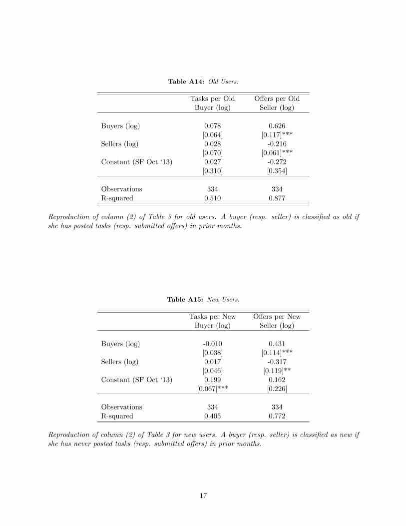
Table A14: Old Users.

Tasks per OldBuyer (log)

O↵ers per OldSeller (log)

Buyers (log) 0.078 0.626[0.064] [0.117]***

Sellers (log) 0.028 -0.216[0.070] [0.061]***

Constant (SF Oct ‘13) 0.027 -0.272[0.310] [0.354]


Reproduction of column (2) of Table 3 for old users. A buyer (resp. seller) is classified as old ifshe has posted tasks (resp. submitted o↵ers) in prior months.

Table A15: New Users.

Tasks per NewBuyer (log)

O↵ers per NewSeller (log)

Buyers (log) -0.010 0.431[0.038] [0.114]***

Sellers (log) 0.017 -0.317[0.046] [0.119]**

Constant (SF Oct ‘13) 0.199 0.162[0.067]*** [0.226]


Reproduction of column (2) of Table 3 for new users. A buyer (resp. seller) is classified as new ifshe has never posted tasks (resp. submitted o↵ers) in prior months.

17

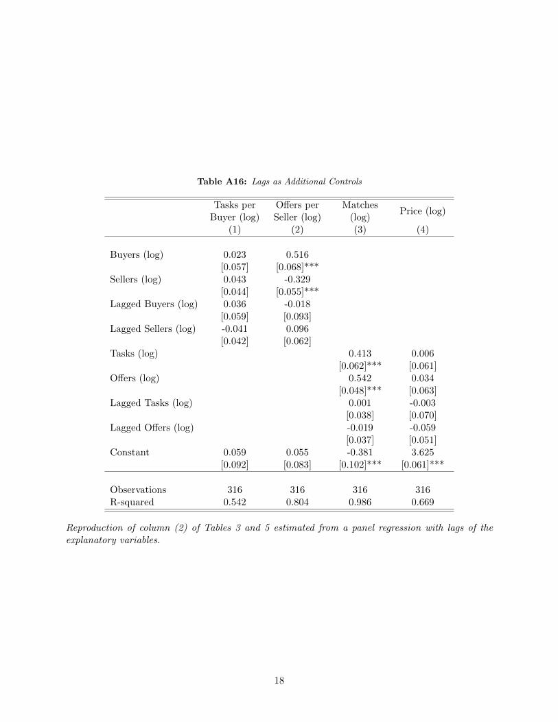
Table A16: Lags as Additional Controls

Tasks perBuyer (log)

O↵ers perSeller (log)

Matches(log)

Price (log)

(1) (2) (3) (4)

Buyers (log) 0.023 0.516[0.057] [0.068]***

Sellers (log) 0.043 -0.329[0.044] [0.055]***

Lagged Buyers (log) 0.036 -0.018[0.059] [0.093]

Lagged Sellers (log) -0.041 0.096[0.042] [0.062]

Tasks (log) 0.413 0.006[0.062]*** [0.061]

O↵ers (log) 0.542 0.034[0.048]*** [0.063]

Lagged Tasks (log) 0.001 -0.003[0.038] [0.070]

Lagged O↵ers (log) -0.019 -0.059[0.037] [0.051]

Constant 0.059 0.055 -0.381 3.625[0.092] [0.083] [0.102]*** [0.061]***


Reproduction of column (2) of Tables 3 and 5 estimated from a panel regression with lags of theexplanatory variables.

18

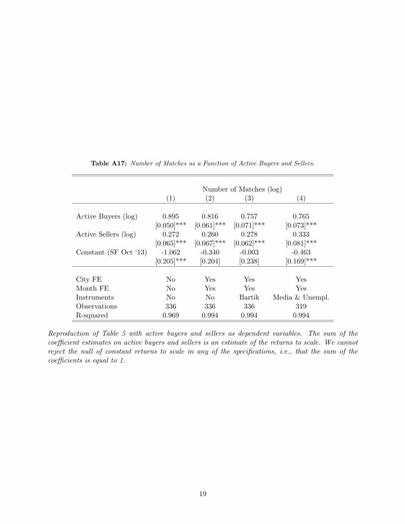
Table A17: Number of Matches as a Function of Active Buyers and Sellers.

Number of Matches (log)(1) (2) (3) (4)

Active Buyers (log) 0.895 0.816 0.757 0.765[0.050]*** [0.061]*** [0.071]*** [0.073]***

Active Sellers (log) 0.272 0.260 0.278 0.333[0.065]*** [0.067]*** [0.062]*** [0.081]***

Constant (SF Oct ‘13) -1.062 -0.340 -0.003 -0.463[0.205]*** [0.204] [0.238] [0.169]***

City FE No Yes Yes YesMonth FE No Yes Yes YesInstruments No No Bartik Media & Unempl.Observations 336 336 336 319R-squared 0.969 0.994 0.994 0.994

Reproduction of Table 5 with active buyers and sellers as dependent variables. The sum of thecoe�cient estimates on active buyers and sellers is an estimate of the returns to scale. We cannotreject the null of constant returns to scale in any of the specifications, i.e., that the sum of thecoe�cients is equal to 1.

19

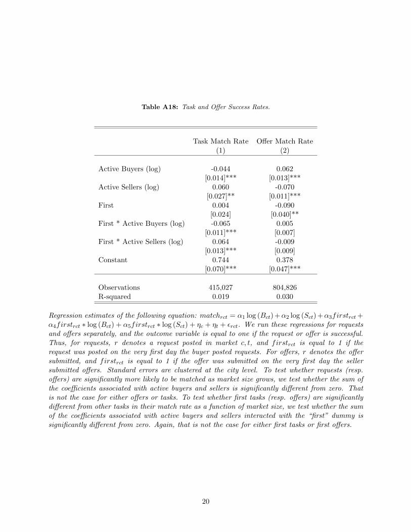
Table A18: Task and O↵er Success Rates.

Task Match Rate O↵er Match Rate(1) (2)

Active Buyers (log) -0.044 0.062[0.014]*** [0.013]***

Active Sellers (log) 0.060 -0.070[0.027]** [0.011]***

First 0.004 -0.090[0.024] [0.040]**

First * Active Buyers (log) -0.065 0.005[0.011]*** [0.007]

First * Active Sellers (log) 0.064 -0.009[0.013]*** [0.009]

Constant 0.744 0.378[0.070]*** [0.047]***

Observations 415,027 804,826R-squared 0.019 0.030

Regression estimates of the following equation: matchrct = ↵1 log (Bct)+↵2 log (Sct)+↵3firstrct+↵4firstrct ⇤ log (Bct) + ↵5firstrct ⇤ log (Sct) + ⌘c + ⌘t + ✏rct. We run these regressions for requestsand o↵ers separately, and the outcome variable is equal to one if the request or o↵er is successful.Thus, for requests, r denotes a request posted in market c, t, and firstrct is equal to 1 if therequest was posted on the very first day the buyer posted requests. For o↵ers, r denotes the o↵ersubmitted, and firstrct is equal to 1 if the o↵er was submitted on the very first day the sellersubmitted o↵ers. Standard errors are clustered at the city level. To test whether requests (resp.o↵ers) are significantly more likely to be matched as market size grows, we test whether the sum ofthe coe�cients associated with active buyers and sellers is significantly di↵erent from zero. Thatis not the case for either o↵ers or tasks. To test whether first tasks (resp. o↵ers) are significantlydi↵erent from other tasks in their match rate as a function of market size, we test whether the sumof the coe�cients associated with active buyers and sellers interacted with the “first” dummy issignificantly di↵erent from zero. Again, that is not the case for either first tasks or first o↵ers.

20

A3 Appendix: Estimates of the Pricing and Matching Functions

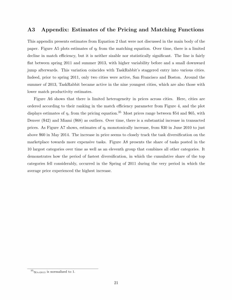
This appendix presents estimates from Equation 2 that were not discussed in the main body of the

paper. Figure A5 plots estimates of ⌘t from the matching equation. Over time, there is a limited

decline in match e�ciency, but it is neither sizable nor statistically significant. The line is fairly

flat between spring 2011 and summer 2013, with higher variability before and a small downward

jump afterwards. This variation coincides with TaskRabbit’s staggered entry into various cities.

Indeed, prior to spring 2011, only two cities were active, San Francisco and Boston. Around the

summer of 2013, TaskRabbit became active in the nine youngest cities, which are also those with

lower match productivity estimates.

Figure A6 shows that there is limited heterogeneity in prices across cities. Here, cities are

ordered according to their ranking in the match e�ciency parameter from Figure 4, and the plot

displays estimates of ⌘c from the pricing equation.35 Most prices range between $54 and $65, with

Denver ($42) and Miami ($68) as outliers. Over time, there is a substantial increase in transacted

prices. As Figure A7 shows, estimates of ⌘t monotonically increase, from $30 in June 2010 to just

above $60 in May 2014. The increase in price seems to closely track the task diversification on the

marketplace towards more expensive tasks. Figure A8 presents the share of tasks posted in the

10 largest categories over time as well as an eleventh group that combines all other categories. It

demonstrates how the period of fastest diversification, in which the cumulative share of the top

categories fell considerably, occurred in the Spring of 2011 during the very period in which the

average price experienced the highest increase.

35⌘Oct2013 is normalized to 1.

21

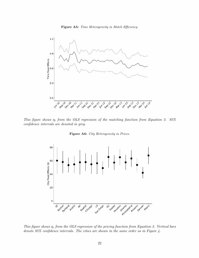
Figure A5: Time Heterogeneity in Match E�ciency.

This figure shows ⌘t from the OLS regression of the matching function from Equation 2. 95%confidence intervals are denoted in grey.

Figure A6: City Heterogeneity in Prices.

This figure shows ⌘c from the OLS regression of the pricing function from Equation 2. Vertical barsdenote 95% confidence intervals. The cities are shown in the same order as in Figure 4.

22

Figure A7: Time Heterogeneity in Prices.

This figure shows ⌘t from the OLS regression of the pricing function from Equation 2. 95% confi-dence intervals are denoted in grey.

23

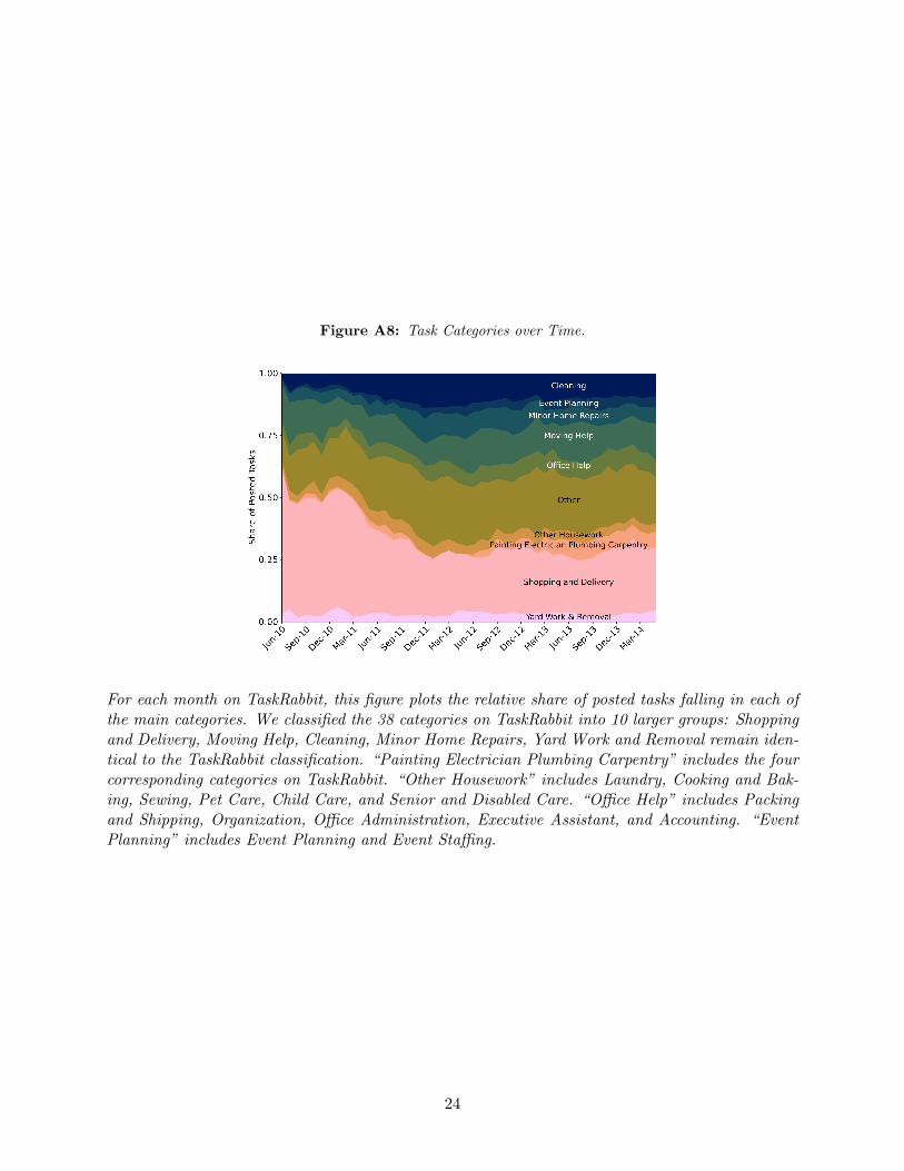
Figure A8: Task Categories over Time.

For each month on TaskRabbit, this figure plots the relative share of posted tasks falling in each ofthe main categories. We classified the 38 categories on TaskRabbit into 10 larger groups: Shoppingand Delivery, Moving Help, Cleaning, Minor Home Repairs, Yard Work and Removal remain iden-tical to the TaskRabbit classification. “Painting Electrician Plumbing Carpentry” includes the fourcorresponding categories on TaskRabbit. “Other Housework” includes Laundry, Cooking and Bak-ing, Sewing, Pet Care, Child Care, and Senior and Disabled Care. “O�ce Help” includes Packingand Shipping, Organization, O�ce Administration, Executive Assistant, and Accounting. “EventPlanning” includes Event Planning and Event Sta�ng.

24

A4 Appendix: Adoption and Retention

This appendix provides estimates of Equations 3 and 4, as well as two ways in which we can use

these estimates to justify our strategy from Section 4. Figure A9 plots buyer adoption and retention

patterns over time.

First, we describe the results from Equation 3. Table A19 shows the estimates of �c, which

highlight major heterogeneity across cities in the rate of platform adoption. We can use these

estimates to verify that deviations from the linear trend in buyer adoption are not correlated with

contemporaneous market conditions, supporting the assumptions underlying the analysis in Section

4. To do this, we take the residuals from Equation 3 and run the following regression:

✏ct = �Xct + �c + �t + ⇠ct,

where Xct is a two-element vector of relevant outcomes in city-month c, t: realized buyer match

rate and average transacted price. As Table A20 shows, the estimates of � are not statistically

significant, nor even of the expected sign.

Second, we use Equation 4 to provide additional support to Section 4. Specifically, we verify

that, if current matches and prices hold, expectations of future outcomes do not a↵ect the propensity

to stay or leave the marketplace. To do this, we run OLS regressions similar to Equation 4:

log

✓stayct

1� stayct

◆= ✓0Xct + ✓1Xt+1,c + ✓2Xt+2,c + ✓3Xt+3,c + ✓t + ✓c + ✏ct,

where Xct is defined as in Equation 4 and includes the current realized match rate and trans-

action price. The regression is run separately for buyers and sellers, so the match rate for buyers

is the task success probability, while the match rate for sellers is the o↵er acceptance rate. The

six-element vector (Xt+1,c, Xt+2,c, Xt+3,c) contains the realized match rates and prices in the fol-

lowing three months within the same city. If users do not base their decision to stay or leave the

marketplace on expectations of future outcomes, we would expect the six-element coe�cient vector

(✓1, ✓2, ✓3) to be non-significant, both for buyers and for sellers.

The results are presented in Tables A21 (for buyers) and A22 (for sellers). Each table has

four columns, which correspond to four di↵erent specifications. The first specification estimates ✓0

without including forward variables–this is precisely Equation 4 from Section 5. Each subsequent

specification sequentially adds the outcomes of the following month, then two months ahead, and

three months ahead. The final column is the full specification. With the exception of just one

coe�cient in the buyers’ regression (the coe�cient on the three-month-ahead transacted price), all

25

other coe�cients from (✓1, ✓2, ✓3) are not statistically di↵erent from zero, and in some cases even

have the opposite sign. Despite the small number of observations, note that users appear to base

their decisions to stay on the marketplace on the contemporaneous match rate more so than other

aspects. Adding forward variables does not change the e↵ect of match rate nor does it help to

improve the goodness of fit of the estimation.

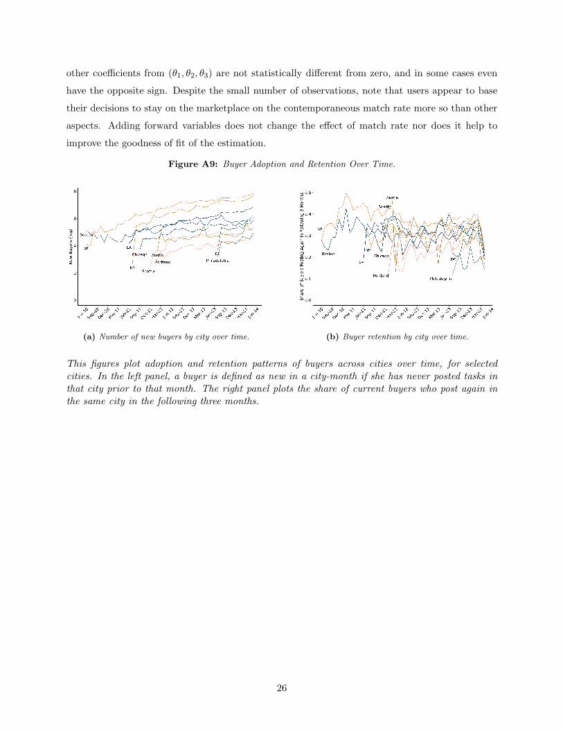
Figure A9: Buyer Adoption and Retention Over Time.

(a) Number of new buyers by city over time. (b) Buyer retention by city over time.

This figures plot adoption and retention patterns of buyers across cities over time, for selectedcities. In the left panel, a buyer is defined as new in a city-month if she has never posted tasks inthat city prior to that month. The right panel plots the share of current buyers who post again inthe same city in the following three months.

26

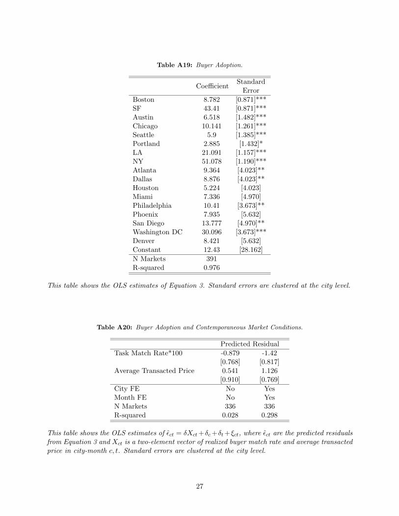
Table A19: Buyer Adoption.

Coe�cientStandardError

Boston 8.782 [0.871]***SF 43.41 [0.871]***Austin 6.518 [1.482]***Chicago 10.141 [1.261]***Seattle 5.9 [1.385]***Portland 2.885 [1.432]*LA 21.091 [1.157]***NY 51.078 [1.190]***Atlanta 9.364 [4.023]**Dallas 8.876 [4.023]**Houston 5.224 [4.023]Miami 7.336 [4.970]Philadelphia 10.41 [3.673]**Phoenix 7.935 [5.632]San Diego 13.777 [4.970]**Washington DC 30.096 [3.673]***Denver 8.421 [5.632]Constant 12.43 [28.162]N Markets 391R-squared 0.976

This table shows the OLS estimates of Equation 3. Standard errors are clustered at the city level.

Table A20: Buyer Adoption and Contemporaneous Market Conditions.

Predicted ResidualTask Match Rate*100 -0.879 -1.42

[0.768] [0.817]Average Transacted Price 0.541 1.126

[0.910] [0.769]City FE No YesMonth FE No YesN Markets 336 336R-squared 0.028 0.298

This table shows the OLS estimates of ✏ct = �Xct+�c+�t+⇠ct, where ✏ct are the predicted residualsfrom Equation 3 and Xct is a two-element vector of realized buyer match rate and average transactedprice in city-month c, t. Standard errors are clustered at the city level.

27

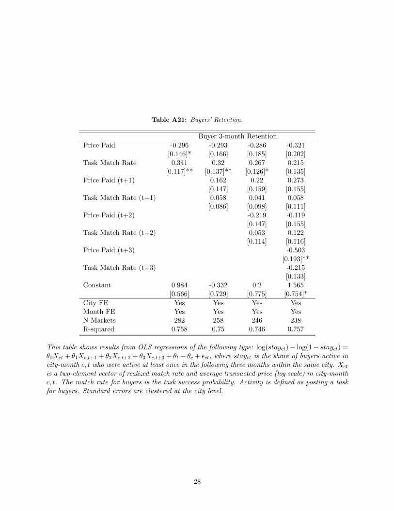
Table A21: Buyers’ Retention.

Buyer 3-month RetentionPrice Paid -0.296 -0.293 -0.286 -0.321

[0.146]* [0.166] [0.185] [0.202]Task Match Rate 0.341 0.32 0.267 0.215

[0.117]** [0.137]** [0.126]* [0.135]Price Paid (t+1) 0.162 0.22 0.273

[0.147] [0.159] [0.155]Task Match Rate (t+1) 0.058 0.041 0.058

[0.086] [0.098] [0.111]Price Paid (t+2) -0.219 -0.119

[0.147] [0.155]Task Match Rate (t+2) 0.053 0.122

[0.114] [0.116]Price Paid (t+3) -0.503

[0.193]**Task Match Rate (t+3) -0.215

[0.133]Constant 0.984 -0.332 0.2 1.565

[0.566] [0.729] [0.775] [0.754]*City FE Yes Yes Yes YesMonth FE Yes Yes Yes YesN Markets 282 258 246 238R-squared 0.758 0.75 0.746 0.757

This table shows results from OLS regressions of the following type: log(stayct)� log(1� stayct) =✓0Xct + ✓1Xc,t+1 + ✓2Xc,t+2 + ✓3Xc,t+3 + ✓t + ✓c + ✏ct, where stayct is the share of buyers active incity-month c, t who were active at least once in the following three months within the same city. Xct

is a two-element vector of realized match rate and average transacted price (log scale) in city-monthc, t. The match rate for buyers is the task success probability. Activity is defined as posting a taskfor buyers. Standard errors are clustered at the city level.

28

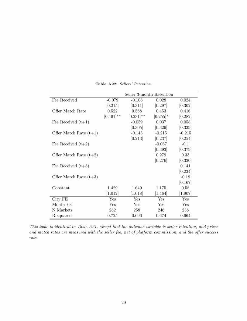
Table A22: Sellers’ Retention.

Seller 3-month RetentionFee Received -0.079 -0.108 0.028 0.024

[0.215] [0.311] [0.297] [0.302]O↵er Match Rate 0.522 0.588 0.453 0.416

[0.191]** [0.231]** [0.255]* [0.282]Fee Received (t+1) -0.059 0.037 0.058

[0.305] [0.329] [0.339]O↵er Match Rate (t+1) -0.143 -0.215 -0.215

[0.213] [0.237] [0.254]Fee Received (t+2) -0.067 -0.1

[0.393] [0.379]O↵er Match Rate (t+2) 0.279 0.33

[0.276] [0.320]Fee Received (t+3) 0.141

[0.234]O↵er Match Rate (t+3) -0.18

[0.167]Constant 1.429 1.649 1.175 0.58

[1.012] [1.018] [1.464] [1.907]City FE Yes Yes Yes YesMonth FE Yes Yes Yes YesN Markets 282 258 246 238R-squared 0.725 0.696 0.674 0.664

This table is identical to Table A21, except that the outcome variable is seller retention, and pricesand match rates are measured with the seller fee, net of platform commission, and the o↵er successrate.

29

Documents

APPENDIX Outsourcing Tasks Online: Matching Supply and