Application of an Ensemble-Trained Source ApportionmentApproach at a Site Impacted by Multiple Point SourcesMarissa L. Maier,* Sivaraman Balachandran, Stefanie E. Sarnat, Jay R. Turner, James A. Mulholland,and Armistead G. Russell

School of Civil and Environmental Engineering, Georgia Institute of Technology, Atlanta, Georgia 30332, United States

*S Supporting Information

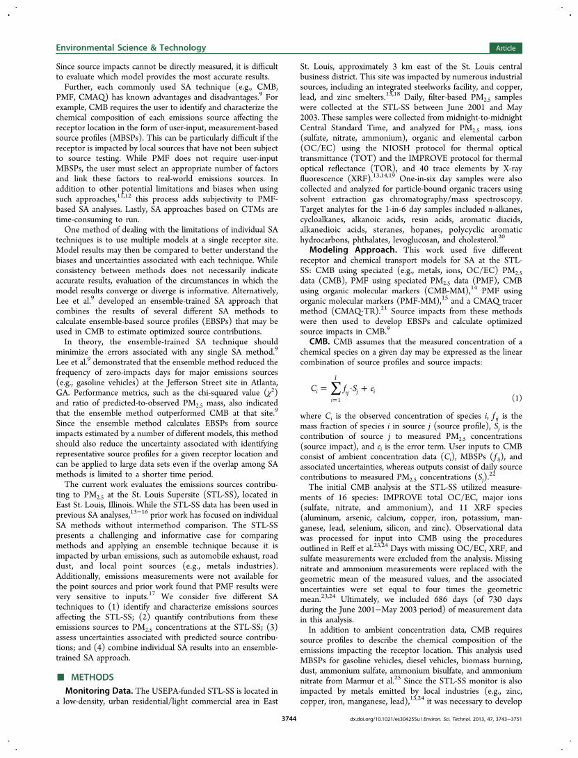
ABSTRACT: Four receptor models and a chemical transportmodel were used to quantify PM2.5 source impacts at the St.Louis Supersite (STL-SS) between June 2001 and May 2003.The receptor models used two semi-independent data sets,with the first including ions and trace elements and the secondincluding 1-in-6 day particle-bound organics. Since each sourceapportionment (SA) technique has limitations, this workcompares results from the five different SA approaches tobetter understand the biases and limitations of each. Thesource impacts calculated by these models were thenintegrated into a constrained, ensemble-trained SA approach.The ensemble method offers several improvements over the five individual SA techniques at the STL-SS. Primarily, the ensemblemethod calculates source impacts on days when individual models either do not converge to a solution or do not have adequateinput data to develop source impact estimates. When compared with a chemical mass balance approach using measurement-based source profiles, the ensemble method improves fit statistics, reducing chi-squared values and improving PM2.5 massreconstruction. Compared to other receptor models, the ensemble method also calculates zero or negative impacts from majoremissions sources (e.g., secondary organic carbon (SOC) and diesel vehicles) for fewer days. One limitation of this analysis wasthat a composite metals profile was used in the ensemble analysis. Although STL-SS is impacted by multiple metals processingpoint sources, several of the initial SA methods could not resolve individual metals processing impacts. The results of this analysisalso reveal some of the subjectivities associated with applying specific SA models at the STL-SS. For instance, Positive MatrixFactorization results are very sensitive to both the fitting species and number of factors selected by the user. Conversely,Chemical Mass Balance results are sensitive to the source profiles used to represent local metals processing emissions.Additionally, the different SA approaches predict different impacts for the same source on a given day, with correlationcoefficients ranging from 0.034 to 0.65 for gasoline vehicles, −0.54−0.48 for diesel vehicles, −0.29−0.81 for dust, −0.34−0.89 forbiomass burning, 0.38−0.49 for metals processing, and −0.25−0.51 for SOC. These issues emphasize the value of using severaldifferent SA techniques at a given receptor site, either by comparing source impacts predicted by different models or by using anensemble-based technique.

■ INTRODUCTION

Epidemiologic studies have linked fine particulate matter(PM2.5) with adverse health outcomes, including cardiovasculardisease and asthma. Ambient PM2.5 is a mixture of pollutantsemitted from multiple sources whose respective contributionsto PM2.5 levels cannot be directly measured. Therefore,scientists and policy-makers are interested in understandinghow individual emissions sources impact PM2.5 concentrationsand human health. Researchers have developed various sourceapportionment (SA) models to quantify the impacts ofemissions sources on pollutant concentrations (e.g., PositiveMatrix Factorization (PMF),1 Chemical Mass Balance (CMB),2

and the Community Multiscale Air Quality Model (CMAQ)3).Some approaches have also been used to provide PM2.5 sourceinputs for epidemiological analyses.4−8 Several issues limit theuse of current SA approaches in epidemiological analyses,particularly those evaluating acute health effects and relying on

day-to-day changes in exposures. Some models appear tointroduce excessive day-to-day variability in source impactestimates whereas other models do the opposite. For example,receptor models, such as PMF and CMB, suggest little-to-no(or even negative) impacts from major emissions sources (e.g.,gasoline vehicles) on certain days and high impacts on otherdays.9 Conversely, SA methods based on chemical transportmodels (CTMs), such as CMAQ, utilize meteorological andemissions inventory data that do not appear to adequatelycapture day-to-day fluctuations in emissions source contribu-tions.5,10 Moreover, different SA techniques tend to predictdifferent PM2.5 impacts for the same source on the same day.9

Received: October 18, 2012Revised: February 20, 2013Accepted: February 26, 2013Published: February 26, 2013

Article

pubs.acs.org/est

© 2013 American Chemical Society 3743 dx.doi.org/10.1021/es304255u | Environ. Sci. Technol. 2013, 47, 3743−3751

Since source impacts cannot be directly measured, it is difficultto evaluate which model provides the most accurate results.Further, each commonly used SA technique (e.g., CMB,

PMF, CMAQ) has known advantages and disadvantages.9 Forexample, CMB requires the user to identify and characterize thechemical composition of each emissions source affecting thereceptor location in the form of user-input, measurement-basedsource profiles (MBSPs). This can be particularly difficult if thereceptor is impacted by local sources that have not been subjectto source testing. While PMF does not require user-inputMBSPs, the user must select an appropriate number of factorsand link these factors to real-world emissions sources. Inaddition to other potential limitations and biases when usingsuch approaches,11,12 this process adds subjectivity to PMF-based SA analyses. Lastly, SA approaches based on CTMs aretime-consuming to run.One method of dealing with the limitations of individual SA

techniques is to use multiple models at a single receptor site.Model results may then be compared to better understand thebiases and uncertainties associated with each technique. Whileconsistency between methods does not necessarily indicateaccurate results, evaluation of the circumstances in which themodel results converge or diverge is informative. Alternatively,Lee et al.9 developed an ensemble-trained SA approach thatcombines the results of several different SA methods tocalculate ensemble-based source profiles (EBSPs) that may beused in CMB to estimate optimized source contributions.In theory, the ensemble-trained SA technique should

minimize the errors associated with any single SA method.9

Lee et al.9 demonstrated that the ensemble method reduced thefrequency of zero-impacts days for major emissions sources(e.g., gasoline vehicles) at the Jefferson Street site in Atlanta,GA. Performance metrics, such as the chi-squared value (χ2)and ratio of predicted-to-observed PM2.5 mass, also indicatedthat the ensemble method outperformed CMB at that site.9

Since the ensemble method calculates EBSPs from sourceimpacts estimated by a number of different models, this methodshould also reduce the uncertainty associated with identifyingrepresentative source profiles for a given receptor location andcan be applied to large data sets even if the overlap among SAmethods is limited to a shorter time period.The current work evaluates the emissions sources contribu-

ting to PM2.5 at the St. Louis Supersite (STL-SS), located inEast St. Louis, Illinois. While the STL-SS data has been used inprevious SA analyses,13−16 prior work has focused on individualSA methods without intermethod comparison. The STL-SSpresents a challenging and informative case for comparingmethods and applying an ensemble technique because it isimpacted by urban emissions, such as automobile exhaust, roaddust, and local point sources (e.g., metals industries).Additionally, emissions measurements were not available forthe point sources and prior work found that PMF results werevery sensitive to inputs.17 We consider five different SAtechniques to (1) identify and characterize emissions sourcesaffecting the STL-SS; (2) quantify contributions from theseemissions sources to PM2.5 concentrations at the STL-SS; (3)assess uncertainties associated with predicted source contribu-tions; and (4) combine individual SA results into an ensemble-trained SA approach.

■ METHODSMonitoring Data. The USEPA-funded STL-SS is located in

a low-density, urban residential/light commercial area in East

St. Louis, approximately 3 km east of the St. Louis centralbusiness district. This site was impacted by numerous industrialsources, including an integrated steelworks facility, and copper,lead, and zinc smelters.13,18 Daily, filter-based PM2.5 sampleswere collected at the STL-SS between June 2001 and May2003. These samples were collected from midnight-to-midnightCentral Standard Time, and analyzed for PM2.5 mass, ions(sulfate, nitrate, ammonium), organic and elemental carbon(OC/EC) using the NIOSH protocol for thermal opticaltransmittance (TOT) and the IMPROVE protocol for thermaloptical reflectance (TOR), and 40 trace elements by X-rayfluorescence (XRF).13,14,19 One-in-six day samples were alsocollected and analyzed for particle-bound organic tracers usingsolvent extraction gas chromatography/mass spectroscopy.Target analytes for the 1-in-6 day samples included n-alkanes,cycloalkanes, alkanoic acids, resin acids, aromatic diacids,alkanedioic acids, steranes, hopanes, polycyclic aromatichydrocarbons, phthalates, levoglucosan, and cholesterol.20

Modeling Approach. This work used five differentreceptor and chemical transport models for SA at the STL-SS: CMB using speciated (e.g., metals, ions, OC/EC) PM2.5data (CMB), PMF using speciated PM2.5 data (PMF), CMBusing organic molecular markers (CMB-MM),14 PMF usingorganic molecular markers (PMF-MM),15 and a CMAQ tracermethod (CMAQ-TR).21 Source impacts from these methodswere then used to develop EBSPs and calculate optimizedsource impacts in CMB.9

CMB. CMB assumes that the measured concentration of achemical species on a given day may be expressed as the linearcombination of source profiles and source impacts:

∑= · +=

C f S eii

I

ij j i1 (1)

where Ci is the observed concentration of species i, f ij is themass fraction of species i in source j (source profile), Sj is thecontribution of source j to measured PM2.5 concentrations(source impact), and ei is the error term. User inputs to CMBconsist of ambient concentration data (Ci), MBSPs ( f ij), andassociated uncertainties, whereas outputs consist of daily sourcecontributions to measured PM2.5 concentrations (Sj).

22

The initial CMB analysis at the STL-SS utilized measure-ments of 16 species: IMPROVE total OC/EC, major ions(sulfate, nitrate, and ammonium), and 11 XRF species(aluminum, arsenic, calcium, copper, iron, potassium, man-ganese, lead, selenium, silicon, and zinc). Observational datawas processed for input into CMB using the proceduresoutlined in Reff et al.23,24 Days with missing OC/EC, XRF, andsulfate measurements were excluded from the analysis. Missingnitrate and ammonium measurements were replaced with thegeometric mean of the measured values, and the associateduncertainties were set equal to four times the geometricmean.23,24 Ultimately, we included 686 days (of 730 daysduring the June 2001−May 2003 period) of measurement datain this analysis.In addition to ambient concentration data, CMB requires

source profiles to describe the chemical composition of theemissions impacting the receptor location. This analysis usedMBSPs for gasoline vehicles, diesel vehicles, biomass burning,dust, ammonium sulfate, ammonium bisulfate, and ammoniumnitrate from Marmur et al.25 Since the STL-SS monitor is alsoimpacted by metals emitted by local industries (e.g., zinc,copper, iron, manganese, lead),13,24 it was necessary to develop

Environmental Science & Technology Article

dx.doi.org/10.1021/es304255u | Environ. Sci. Technol. 2013, 47, 3743−37513744

representative metals processing profiles for use in CMB.However, source testing data for these specific industrialsources were not available, so metals processing profiles weredeveloped from the composite copper, steel, and leadprocessing profiles in EPA’s Speciate database (Profiles91008, 900042.5, and 293302.5).26 An appropriate profile forthe zinc smelter south of the STL-SS was not identified inSpeciate and was therefore not included in the CMB analysis;however, the lead profile contained approximately 35% zinc bymass. Speciate provided measurement uncertainties for thecomposite lead smelting profile. Uncertainties for the steel andcopper profiles were set equal to 50% of the mass fraction ofeach species. Recognizing that the measurement-based copper,steel, and lead processing profiles (MBSPs with individualmetals profiles or MBSPs-MI) may not fully characterize themetals processing emissions impacting the STL-SS, threeadditional sets of metals processing profiles were developedfor a sensitivity analysis. A composite, measurement-basedmetals processing profile (MBSPs with composite metalsprofiles or MBSPs-MC) was developed as a weighted averageof source profiles and source impacts from the initial CMBresults (CMB-MBSPs-MI or CMB). Individual and compositemetals processing profiles were also developed from the PMFprofiles for industrial lead, copper, zinc, and steel (PMF-MI andPMF-MC).CMB results using MBSPs-MI were incorporated into the

ensemble method; CMB results using MBSPs-MC, PMF-MI,and PMF-MC were compared to the ensemble results. Dailysource impacts and associated uncertainties were calculated inEPA CMB8.2 using an effective variance approach and sourceelimination to prevent negative source impacts.22

PMF. Like CMB, factor analytic methods, such as EPA’sPMF, also assume that the ambient concentration of a chemicalspecies, i, can be expressed as the linear combination of themass of species i in source j and the contribution of source j toPM2.5 concentrations. PMF uses a mathematical approach todecompose sample data into factors and contributions;therefore the user is not responsible for specifying the chemicalcomposition of the emissions sources impacting the monitor.The user must, however, choose an appropriate number offactors and relate these factors to real-world emissions sources.Although the selection of an appropriate number of factors isguided by the use of fitting statistics (e.g., the Q value) thisprocess can still be subjective.The only difference between the concentration and

uncertainty data used in CMB and PMF was the use oftemperature-resolved IMPROVE OC/EC fractions, rather thantotal OC/EC measurements. The analysis also excluded dayswith missing ion measurements, resulting in 655 (of 730) daysof measurement data for input into PMF. Calculations wereperformed using EPA PMF v3.0.2.2.27 Species with signal-to-noise ratios (S/N) less than two were considered weak species:

∑=| |

=

SN

SNk

k

k1

2

2(2)

where S is the signal and N is the noise for each measurement k.The uncertainties associated with these species were multipliedby a factor of 3 to lower their influence on the final 11-factorPMF solution. A bootstrapping analysis was performed toestimate the stability and uncertainty of the PMF solution.Factor contributions were determined from the average of 100

bootstrapping runs, and uncertainties were set equal to thestandard deviation of 100 bootstrapping runs.

Molecular Marker Methods. 1-In-6 day, particle-boundorganic data and the NIOSH OC/EC measurements were usedin both CMB and PMF to estimate source contributions to OCrather than PM2.5 at the STL-SS between June 2001 and May2003. For CMB-MM, we used source contributions to OC,source impact uncertainties, and model fit statistics for 148 (of730) days at the STL-SS reported in Bae et al.14 Since Bae et al.considered all unapportioned OC to be from secondarysources, the model did not calculate source impact uncertaintiesfor SOC.Jaeckels et al.15 previously used PMF-MM to estimate source

contributions to OC concentrations at the STL-SS betweenJune 2001 and May 2003. Since Jaeckels et al. did not providedaily source contributions to OC concentrations, we reranPMF-MM using their input files, which consisted of ambientconcentration data and associated measurement uncertaintiesfor 107 particle-bound organic compounds, NIOSH OC/EC,silicon, and aluminum for 93 (of 730) days.15,28 We added 11days of measurement data to the original data set, including 4days in July 2001. We estimated measurement uncertainties forthe 11 additional days by regressing the initial 93 days ofambient concentration data by their associated measurementuncertainties. Species with S/N less than two were treated as“weak” species and 9-hexadecenoiacid was excluded from theanalysis.15 The resulting eight-factor PMF solution was similarto the eight-factor PMF solution reported by Jaeckels et al.

CMAQ-TR. CMAQ-TR uses the CTM, CMAQ, and thedirect decoupled method in three dimensions to investigate thesensitivity of PM2.5 concentrations to emissions from 28 sourcecategories. Baek et al. previously ran CMAQ-TR for a domaincovering the contiguous United States, for 29 days in July2001and 29 days in January 2002.21 CMAQ-TR does notestimate source impact uncertainties, which is a limitation ofthis method.

Ensemble Method. Ensemble-average source impacts atthe STL-SS were calculated from the PMF, PMF-MM, CMB,CMB-MM, and CMAQ-TR results for July 2001 and January2002. This study considered nine categories of PM2.5 emissions:gasoline vehicle exhaust and resuspended road dust (GV),diesel vehicle exhaust (DV), dust (DUST), biomass burning(BURN), metals processing (METALS), secondary organiccarbon (SOC), secondary sulfate, secondary nitrate, andammonium. These nine source categories comprise about70% of the inventoried primary PM2.5 sources and thedominant sources that contribute to secondary pollutantformation.21 The individual emissions sources identified byCMB, PMF, CMB-MM, PMF-MM, and CMAQ-TR werebinned into the five primary source categories (i.e., GV, DV,BURN, DUST, and METALS) and SOC (see SupportingInformation (SI) Table S1). Secondary sulfate, nitrate, andammonium source categories were estimated using only the 11-factor PMF results. The secondary sulfate and nitrate factorsaccounted for the majority of the modeled sulfate (86%),nitrate (81%), and ammonium (81%) mass in PMF. However,these secondary species were also present at low levels in theprimary source factors (i.e., gasoline vehicles). Thus, secondarysulfate, nitrate, and ammonium contributions were calculatedby summing the modeled sulfate, nitrate, and ammonium massacross the 11 PMF factors. Sulfate was left in the PMF steelprocessing factor, since it comprised a significant percentage(40% by mass) of the steel processing MBSP used in CMB.

Environmental Science & Technology Article

dx.doi.org/10.1021/es304255u | Environ. Sci. Technol. 2013, 47, 3743−37513745

Although PMF did not resolve an SOC factor, the OC in thesecondary sulfate and nitrate factors was considered to be fromsecondary formation. As such, the OC from these two PMFfactors was combined with the SOC estimated by CMAQ-TR,CMB-MM, and PMF-MM to calculate ensemble-average SOCimpacts.PMF-MM and CMB-MM calculate source contributions to

OC rather than PM2.5 mass. Source contributions from thesemethods were scaled by source-specific OC/PM2.5 ratiosprovided in the literature14,29−31 (see SI Table S2). SincePMF-MM did not resolve separate gasoline and diesel vehiclefactors, the combined mobile source factor was split into a

gasoline and diesel component using the ratio of gasoline todiesel vehicle impacts estimated in CMAQ-TR.Ensemble-average source impacts were calculated by

averaging the daily source impacts predicted by each modelfor two one-month periods in July 2001 and January 2002.Since each SA approach uses a different method for estimatingsource impact uncertainties, all methods were given an equalweighting during the averaging. However, to prevent ensemble-average source contributions from being biased by theavailability (or unavailability) of model results on a particularday, source contributions were mean-centered prior toaveraging.

Table 1. Comparison of Average PM2.5 Source Impacts Estimated by CMB, PMF, CMB-MM, PMF-MM, and CMAQ-TR forJune 2001−May 2003

PMFa CMBb CMAQ-TRc PMF-MMa CMB-MMb

%PM2.5 or OC mass ratio, %d 100 ± 12 91 ± 15 77 ± 26e 229 ± 116 84 ± 48g

118 ± 34f

mean measured PM2.5 or OC mass, μg/m3 d 18.0 17.9 22.1e 3.8 3.917.8f

N 655 433h 29e 123 148average PM2.5 source impacts, μg/m3

GV 2.2 ± 1.4 4.0 ± 0.56 2.5 0.62 ± 0.39 5.1 ± 0.65DV 1.4 ± 1.1 0.78 ± 0.56 0.89 0.75 ± 0.48 0.31 ± 0.05DUST 0.96 ± 0.64 0.34 ± 0.17 1.3 1.3 ± 0.61 0.28 ± 0.03BURN 1. ± 0.62 1.2 ± 1.1 3.0 0.64 ± 0.42 1.3 ± 0.28SOC 0.29 ± 0.01 0.21 ± 0.63 1.3 0.59 ± 0.33 1.7c

METALS 1.9 ± 0.97 1.7 ± 0.54 1.0aSource impact uncertainties were calculated from the standard deviation of 100 bootstrapping runs. bSource impact uncertainties were calculated byCMB. cSource impact uncertainties were not calculated by the model. dModeled-to-measured PM2.5 mass ratios and mean measured PM2.5 massprovided for PMF, CMB, and CMAQ-TR. Modeled-to-measured OC mass ratios and mean measured OC (NIOSH/TOT) mass provided for PMF-MM and CMB-MM. eJuly 2001. fJanuary 2002. gDoes not consider SOC. Since Bae et al. considered all unapportioned OC to be from secondarysources, modeled-to-measured mass ratio is 100% with SOC. hCMB failed to converge to a solution on 253 of the 686 days with valid measurementdata.

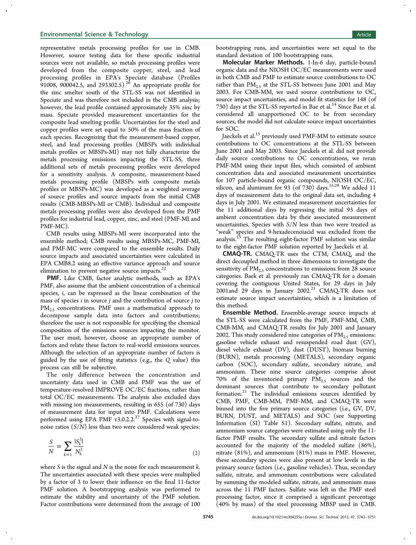
Figure 1. Comparison of ensemble average source impacts in μg/m3 to selected SA results from PMF, CMB, PMF-MM, CMB-MM, and CMAQ-TRfor July 2001 and January 2002: (a) GV, (b) DUST, (c) SOC, (d) METAL.

Environmental Science & Technology Article

dx.doi.org/10.1021/es304255u | Environ. Sci. Technol. 2013, 47, 3743−37513746

The ensemble-average source impacts were used to under-stand how source impacts from each of the five initial SAapproaches deviated from the mean during July 2001 andJanuary 2002:32

∑σ = −=N

S S1

( )jlk

N

jkl jkl2

1

2

(3)

Here, σjl is the deviation of source j from the mean orupdated source impact uncertainty for each SA method l (i.e.,CMB, PMF, CMB-MM, PMF-MM, or CMAQ-TR), Sjkl is theensemble-average impact for source j on day k, Sjkl is thecontribution from source j from method l on day k, and N isthe number of days included in the calculation. N ranged from9 for PMF-MM to 55 for CMAQ-TR and PMF. σjl’s were thencompared to initial uncertainty estimates from PMF and CMBand used for intermethod comparison.Ensemble-average source impacts for July 2001 and January

2002 were then used to calculate summer and winter EBSPs( f ij’s) using a reverse CMB approach that minimized χ2:

∑χσ

=− ∑

=

=C f S( )

i

Nik j

Jij jk

C

2

1

12

2ik (4)

where Cik is the observed concentration of species i on day k, f ijis the mass fraction of species i in source j, Sjk is thecontribution of source j to PM2.5 concentrations on day k, andσCik

2 is the uncertainty associated with the measuredconcentration. Calculations were performed in Excel, using anonlinear solver package developed by Frontline Systems.33

During each optimization, the source profiles were initially setto the MBSPs, and constrained to the MBSP ± 3 × σMBSP aslong as these values were between 0 and 1. Additionally, thetotal mass fractions of the species in the source profiles were

restricted to values less than or equal to one. This calculationspecified a primary organic matter to OC (OM/OC) ratio of1.2 for GV, DV, DUST, and METALS, and an OM/OC ratio of1.4 for BURN. OC/EC ratios for GV and DV were constrainedto values between 0.80 and 4.0 and 0.17 and 1.25,respectively.34 The OC/EC ratio for the BURN profile wasconstrained to values greater than or equal to 3. Lastly, the totalcarbon fractions (OC + EC) in the GV, DV, and BURNprofiles were constrained to values greater than or equal to 0.5.Daily source profiles were averaged for July 2001 and January

2002 to calculate the summer and winter EBSPs. The sourceprofile uncertainties were set equal to the standard deviation ofthe daily profiles. The summer profiles were used to estimatesource impacts in CMB between April and October, while thewinter profiles were applied to daily measurements collectedbetween November and March.

■ RESULTS AND DISCUSSION

A comparison of the CMB, PMF, CMAQ-TR, CMB-MM, andPMF-MM results demonstrate that these techniques cancalculate very different source impacts for the same receptorlocation (Table 1, Figure 1). Pairwise Pearson correlationcoefficients between the five methods ranged 0.034−0.65 forGV, −0.54−0.48 for DV, −0.29−0.81 for DUST, −0.34−0.89for biomass burning, −0.25−0.51 for SOC, and 0.38−0.49 forMETALS (see SI Tables S3A−G). Correlation coefficientsbetween CMB and PMF ranged from 0.11 for SOC to 0.81 forDUST, whereas correlation coefficients between CMB-MMand PMF-MM ranged from 0.10 for SOC to 0.89 for BURN.PMF, CMB, PMF-MM, CMB-MM, and CMAQ-TR results

were then combined to calculate ensemble-average sourceimpacts for July 2001 and January 2002 (Figure 1). Since theensemble method used information from five differentmethods, source impacts could be resolved on days when

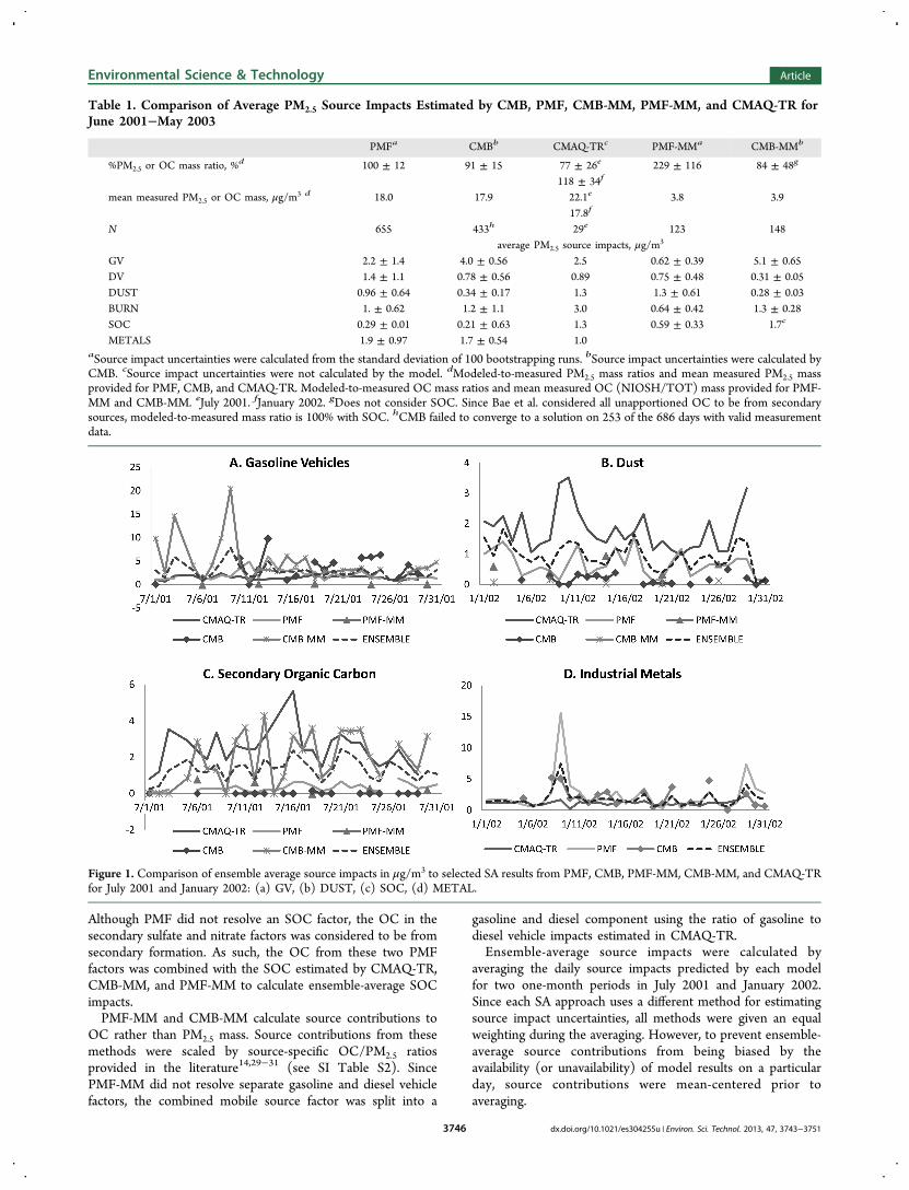
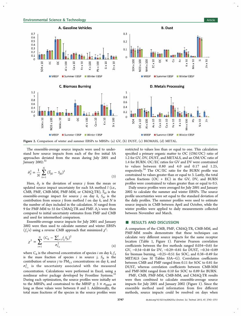
Figure 2. Comparison of winter and summer EBSPs to MBSPs: (a) GV, (b) DUST, (c) BIOMASS, (d) METAL.

Environmental Science & Technology Article

dx.doi.org/10.1021/es304255u | Environ. Sci. Technol. 2013, 47, 3743−37513747

individual methods did not provide results. This was animprovement over CMB, which failed to converge to a solutionon over 35% of the 686 days with valid measurements (due tocolinearity between source profiles), and the molecular markersmethods, which only had adequate sample data to resolvesource impacts on approximately one-sixth of the days duringthe time period of interest (Table 1). The ensemble methodalso eliminated negative and zero impact estimates for majoremissions sources, such as vehicles and SOC. This was an issuefor both the CMB- and PMF-based methods. CMB, forexample, calculated no impact from DV on 141 days and noimpact from SOC on 336 days between June 2001 and May2003, including during the summer.CMAQ-TR and ensemble results generally exhibited less

day-to-day variability in source impacts than the other receptor-based approaches. For example, CMB-MM calculated spikes inGV impacts on 7/3/2001 (14.6 μg/m3) and 7/9/2001 (20.4μg/m3). While the ensemble method also calculated elevatedGV impacts for these days (5.9 and 7.9 μg/m3 on 7/3/2001and 7/9/2001, respectively), they were lower than thoseestimated by CMB-MM. A similar dampening effect wasobserved for the ensemble-average DV, DUST, and BURNimpacts in July (results not shown). Conversely, the ensembleresults for the composite metals processing source exhibited theday-to-day variability expected from a point source orcombination of point sources. CMAQ-TR, however, did notcapture the elevated metals processing impacts estimated byother methods in July and January (e.g., July 10 and January 9).Prior to developing summer and winter EBSPs, the

ensemble-average source impacts were used to understandhow source impacts for the five initial SA methods deviatedfrom the mean in July 2001 and January 2002 (eq 3). Thistechnique provides uncertainty estimates for SA methods thatdid not previously calculate source impact uncertainties (i.e.,CMAQ-TR and SOC in CMB-MM). Additionally, sincedifferent methods use different techniques to calculateuncertainties (e.g., bootstrapping, effective variance), σjl allowedfor a better comparison between methods. Updated relativeuncertainties, defined as the deviation from the mean dividedby the average source impact (σ/S ), range 0.49−6.9 for CMB,0.57−2.6 for PMF, 0.66−4.4 for CMB-MM, 0.46−20 for PMF-MM, and 0.49−1.2 for CMAQ-TR (SI Tables S4A−F). σjl’swere generally higher than the source impact uncertainties

calculated in CMB and PMF. However, σjl was lower than theinitial source impact uncertainty for PMF for DV and METAL(SI Tables S4A−F).Ensemble-average source impacts for July 2001 and January

2002 were then used to calculate summer and winter EBSPs,using a constrained inverse CMB model (eq 4). In general, theEBSPs and MBSPs-MI showed greater interprofile variability inthe weight percentages of the XRF species than the ionicspecies, EC, and OC (Figure 2). The EC/OC ratios and totalcarbon fractions for the ensemble- and measurement-based GVand DV profiles were identical to two significant figures. EC/OC ratios were 0.43 for the GV profiles and 3.7 for the DVprofiles. It should be noted that DV profile EC/OC ratiosreflect vehicles moving at intermediate to highway speeds, butmay vary substantially depending upon operational mode.35

The ensemble-based DUST and BURN profiles containedsmaller mass fractions of most XRF species than the MBSPs,particularly Si, Al, and K (Figure 2). The 16 fitting species usedin this analysis also tended to explain a smaller mass fraction ofthe EBSPs than the MBSPs. For example, the MBSPsaccounted for 92% of the mass of the DUST source, whereasthe summer and winter EBSPs accounted for 89% and 84% ofthe DUST source.The greatest differences between the EBSPs and MBSPs

were observed for the metals processing source. This wasexpected, since the metals processing source was a composite ofmultiple industrial point sources, and the composition of thissource was expected to be more variable than the other sources.For example, the METALS EBSPs contained substantially lessAs, Si, and Zn than the METALS MBSP. As with the othersources, the 16 fitting species accounted for a smaller massfraction of the METALS EBSPs than the METALS MBSP. Thesummer and winter EBSPs explained 33% and 31% of theMETALS profile mass, while the METALS MBSP explained71%. The finding that the EBSPs consistently explained less ofthe emissions source mass than the MBSPs is due, in part, tothe lower bound on the total mass fraction of the EBSPs beingunconstrained.The summer and winter EBSPs were used to calculate

optimized source impacts at the STL-SS between June 2001and May 2003 using CMB (CMB-EBSPs). Correlationcoefficients between source impacts estimated using CMB-EBSPs and the five initial SA methods ranged 0.16−0.66 for

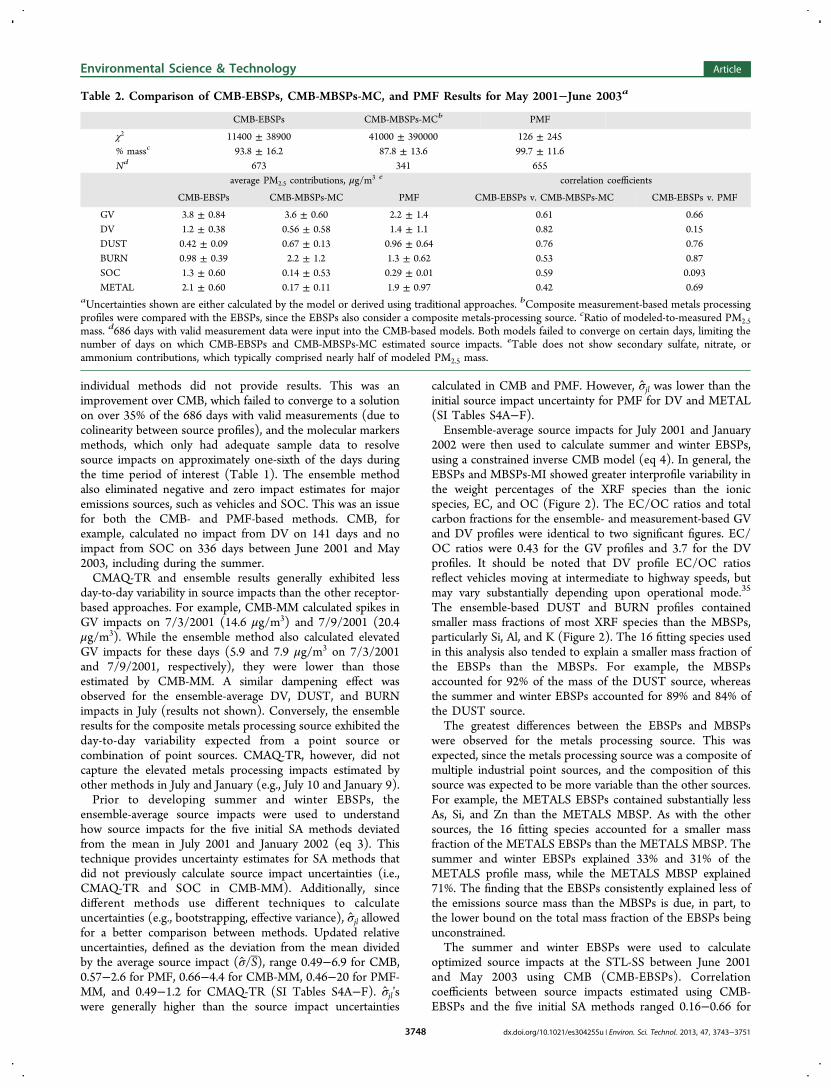
Table 2. Comparison of CMB-EBSPs, CMB-MBSPs-MC, and PMF Results for May 2001−June 2003a

CMB-EBSPs CMB-MBSPs-MCb PMF

χ2 11400 ± 38900 41000 ± 390000 126 ± 245% massc 93.8 ± 16.2 87.8 ± 13.6 99.7 ± 11.6Nd 673 341 655

average PM2.5 contributions, μg/m3 e correlation coefficients

CMB-EBSPs CMB-MBSPs-MC PMF CMB-EBSPs v. CMB-MBSPs-MC CMB-EBSPs v. PMF

GV 3.8 ± 0.84 3.6 ± 0.60 2.2 ± 1.4 0.61 0.66DV 1.2 ± 0.38 0.56 ± 0.58 1.4 ± 1.1 0.82 0.15DUST 0.42 ± 0.09 0.67 ± 0.13 0.96 ± 0.64 0.76 0.76BURN 0.98 ± 0.39 2.2 ± 1.2 1.3 ± 0.62 0.53 0.87SOC 1.3 ± 0.60 0.14 ± 0.53 0.29 ± 0.01 0.59 0.093METAL 2.1 ± 0.60 0.17 ± 0.11 1.9 ± 0.97 0.42 0.69

aUncertainties shown are either calculated by the model or derived using traditional approaches. bComposite measurement-based metals processingprofiles were compared with the EBSPs, since the EBSPs also consider a composite metals-processing source. cRatio of modeled-to-measured PM2.5mass. d686 days with valid measurement data were input into the CMB-based models. Both models failed to converge on certain days, limiting thenumber of days on which CMB-EBSPs and CMB-MBSPs-MC estimated source impacts. eTable does not show secondary sulfate, nitrate, orammonium contributions, which typically comprised nearly half of modeled PM2.5 mass.

Environmental Science & Technology Article

dx.doi.org/10.1021/es304255u | Environ. Sci. Technol. 2013, 47, 3743−37513748

GV, 0.02−0.85 for DV, −0.19−0.86 for DUST, 0.07−0.87 forBURN, −0.22−0.72 for SOC, and 0.21−0.69 for METALS (seeSI Tables S3A−G). The metals processing impacts estimatedby PMF and CMB were better correlated with impactsestimated using the ensemble method than with impactsestimated using CMAQ-TR. This result was expected since theemissions inventory and meteorological data used in CMAQ-TR are thought to underestimate day-to-day variability in localpoint source emissions and pollutant transport to the receptor.5

CMB-EBSPs offered several advantages over CMB-MBSPs.Primarily, CMB-EBSPs calculated source impacts on more daysthan CMB-MBSPs. CMB-EBSPs also reduced zero impact daysfor major emissions sources, such as DV and SOC. Further,goodness of fit statistics, such as χ2 and the ratio of modeled-to-measured PM2.5 mass, were improved using CMB-EBSPs.CMB-EBSPs also resulted in a higher estimate of averagemetals processing impacts and the fewest zero impact days forthis source (Table 2). This indicates that PM2.5 from industrialpoint sources impacted the STL-SS on most days during thetime period of interest, which is likely due to the proximity ofthose sources; however, this result could also indicate thatCMB-EBSPs apportion too much PM2.5 mass to the compositeindustrial metals source. The ensemble technique offers analternative method for developing representative metalsprocessing profiles. This is advantageous since the speciateMBSPs may not adequately characterize the industrial pointsources affecting the STL-SS due to operational differencesbetween facilities (e.g., furnace types, purity of the raw material,emissions controls) and other factors. For example, the steelMBSP was approximately 40% sulfate; however, a comparisonof sulfate concentrations measured near the steel facility fenceline (Granite City Monitor) and at a distal monitor (BlairStreet) does not indicate primary sulfate impacts from thefacility.36 Lastly, while the MBSPs did not consider the nearbyzinc smelter, the metal EBSPs contain information from theindustrial zinc factor identified during the PMF analysis.Compared to CMB-EBSPs, PMF had a better modeled-to-

measured PM2.5 mass ratio and lower χ2. This is expected sincePMF adjusts source profiles to improve fit over the entire timeperiod. However, there are still several advantages to theconstrained ensemble method, which considers informationfrom multiple SA models, including PMF. First, PMF requiresseveral semisubjective decisions, such as selecting an appro-priate number of factors and relating these factors to real-worldemissions sources. For example, a previous PMF analysis at theSTL-SS found that ten factors produced a robust solution,which corresponded well with known PM2.5 sources in East St.Louis.13 The current study found that an additional factor (11factors) was required to distinguish gasoline from diesel vehicleimpacts. Additionally, this work found that the PMF resultswere sensitive to the selection of XRF fitting species, especiallyin the resolution of separate gasoline and diesel vehicle factors.Similarly, Christensen and Schauer found that the gasolinefactor was the least stable PMF factor for this data set.12 Incontrast, the ensemble method utilizes gasoline and dieselvehicle profiles developed from the results of several differentSA methods, circumventing some of the issues associated withdistinguishing mobile source factors. Lastly, the ensemblemethod does not rely on fractionated OC/EC data, which maynot be available for all receptor locations of interest (e.g., earlierChemical Speciation Network data).While the ensemble method offers several advantages over

other SA approaches at the STL-SS, this method is also subject

to several limitations. First, CMB-EBSPs used a compositemetals processing source to incorporate the CMAQ-TR results,which consider only industry-wide impacts. Since the smeltersare located south of the site and the steelworks is located northof the site, impacts from these sources may not always covaryand the composite METALS profile may not adequatelycharacterize industrial metals emissions for all wind directionsand pollutant transport conditions.Additionally, results from a number of different SA methods

are needed to calculate the EBSPs. This makes the ensemblemethod more time-consuming to implement than otherreceptor-based SA techniques, especially if previous SA resultsare unavailable. This work considered five SA models basedprimarily on data availability; however, Lee et al. andBalachandran et al. found that removing individual methodsfrom the ensemble calculation (i.e., CMAQ and CMB-MM)changed predicted source contributions by less than 3%.9

Additionally, while the EBSPs outperform the MBSPs at theSTL-SS based on goodness of fit statistics and reductions inzero impact days, actual source impacts at the STL-SS cannotbe directly measured. Thus, it is impossible to conclusivelydetermine which method is most accurate. However, since theensemble method incorporates results from a number ofdifferent SA strategies, each with its own biases and limitations,this method should limit the inaccuracies associated with anysingle method. Further, Balachandran et al. found thatensemble average source impact uncertainties were lowerthan individual method uncertainties using an iterativeapproach to calculate source impact uncertainties andensemble-average source impacts for the Jefferson St. site inAtlanta.32

In addition to testing the newly developed ensemble-basedSA technique, this work also highlights some of the difficultiesassociated with using traditional SA approaches at a monitorimpacted by multiple point sources. Since the composition ofthe metals processing sources affecting the STL-SS are not well-characterized and the composite METALS EBSP may not fullycapture compositional variations in metals processing emis-sions, a sensitivity analysis was conducted using five differentsets of metals processing profiles: MBSPs-MI, MBSPs-MC,PMF-MI, PMF-MC, and EBSPs. CMB-derived source impactsusing these different profiles were correlated, with correlationcoefficients ranging 0.39−0.93 for GV, 0.80−0.96 for DV,0.53−0.94 for DUST, 0.38−0.85 for BURN, 0.58−0.91 forSOC, and 0.37−0.84 for metals processing (see SI TablesS5A−G). However, average PM2.5 contributions for all sourcesvaried somewhat depending upon the metals processingprofiles. For example, average BURN impacts ranged from0.98 for CMB-EBSPs to 3.4 for CMB-PMF-MC, and averageGV impacts ranged from 2.5 for CMB-PMF-MI to 4.0 forCMB-MBSPs-MI (see SI Table S6). This analysis suggests thatestimated source impacts were somewhat sensitive to the metalprocessing profile or set of profiles, even though metalsprocessing impacts accounted for less than 15% ofreconstructed PM2.5 mass.This sensitivity analysis indicates that decisions made in the

application of the various methods, such as the characterizationof local point sources, can impact SA results. This elucidates thebenefits of using several different SA models since there arelimitations, subjectivities, and uncertainties associated with allavailable approaches. In particular, if the sources impacting aparticular receptor location are not well-characterized, it may beuseful to consider both a factor analytic and a CMB approach.

Environmental Science & Technology Article

dx.doi.org/10.1021/es304255u | Environ. Sci. Technol. 2013, 47, 3743−37513749

PMF allows the user to investigate source impacts at thereceptor site without quantitatively characterizing the compo-sition of important emissions sources. CMB avoids the need toselect an appropriate number of factors and link these factors toreal-world sources. Additionally, while CMAQ-TR results maynot be available for the entire time period of interest, theseresults may be used to understand whether receptor modelresults are consistent with meteorological and emissionsinventory data, and potentially identify emissions inventorydeficiencies. Conversely, receptor models may better character-ize the day-to-day variability in source impacts at a specific sitemissed by CTMs, such as CMAQ. Lastly, organic molecularmarker methods provide SA results using a semi-independentdata set that is not influenced by trace metals; however,molecular marker data are not widely available and must bescaled by source specific PM2.5/OC ratios, adding uncertaintyto the analysis. It is therefore advantageous to use severaldifferent SA techniques at a given receptor site, either bycomparing source impacts predicted by different models usingdifferent data sets or by utilizing an ensemble-trained SAtechnique.

■ ASSOCIATED CONTENT*S Supporting InformationTables S1, S2, S3A−G, S4A−F, S5A−G, and S6, as mentionedin the text. This material is available free of charge via theInternet at http://pubs.acs.org.

■ AUTHOR INFORMATIONCorresponding Author*Phone: (201)704-8609; e-mail: marissalmaier@gmail.com;present address: 820 North Pollard Street, Apt. 208, Arlington,VA 22203.Author ContributionsThe manuscript was written through contributions of allauthors. All authors have given approval to the final version ofthe manuscript.NotesThe authors declare no competing financial interest.

■ ACKNOWLEDGMENTSThis work was supported by the U.S. EPA under GrantsRD833626-01, RD833866, and RD83479901, and SouthernCompany and Georgia Power. Input data for CMB-MM wasprovided by Jaime Schauer at the University of Wisconsin. Wealso thank Jeremiah Redman at the Georgia Institute ofTechnology for his assistance with the ensemble calculations.

■ REFERENCES(1) Paatero, P.; Tapper, U. Positive Matrix Factorization - aNonnegative Factor Model with Optimal Utilization of Error-Estimates of Data Values. Environmetrics 1994, 5 (2), 111−126.(2) Watson, J. G.; Cooper, J. A.; Huntzicker, J. J. The effectivevariance weighting for least squares calculations applied to the massbalance receptor model. Atmos. Environ. 1984, 18, 1347−55.(3) Bruyn, D. W.; Ching, J. K. S. Science Algorithms of the EPA Models-3 Community Multiscale Air Quality (CMAQ) Modeling System;U.S.EPA: Research Triangle Park, NC, 1999.(4) Sarnat, J. A.; Marmur, A.; Klein, M.; Kim, E.; Russell, A. G.;Sarnat, S. E.; Mulholland, J. A.; Hopke, P. K.; Tolbert, P. E. FineParticle Sources and Cardiorespiratory Morbidity: An Application ofChemical Mass Balance and Factor Analytical Source-ApportionmentMethods. Environ. Health Perspect. 2008, 116 (4), 459−466.

(5) Marmur, A.; Park, S.-K.; Mulholland, J. A.; Tolbert, P. E.; Russell,A. G. Source apportionment of PM2.5 in the southeastern UnitedStates using receptor and emissions-based models: Conceptualdifferences and implications for time-series health studies. Atmos.Environ. 2006, 40 (14), 2533−2551.(6) Ito, K.; et al. PM source apportionment and health effects: 2. Aninvestigation of intermethod variability in associations between source-apportioned fine particle mass and daily mortality in Washington DC.J. Exposure Sci. Environ. Epidemiol. 2006, 16 (4), 300−310.(7) Laden, F.; Neas, L. M.; Dockery, D. W.; Schwartz, J. Associationof fine particulate matter from different sources with daily mortality insix US cities. Environ. Health Perspect. 2000, 108 (10), 941−947.(8) Mar, T. F.; et al. PM source apportionment and health effects. 3.Investigation of inter-method variations in associations betweenestimated source contributions Of PM2.5 and daily mortality inPhoenix AZ. J. Exposure Sci. Environ. Epidemiol. 2006, 16 (4), 311−320.(9) Lee, D.; Balachandran, S.; Pachon, J.; Shankaran, R.; Lee, S.;Mulholland, J. A.; Russell, A. G. Ensemble-Trained PM2.5 SourceApportionment Approach for Health Studies. Environ. Sci. Technol.2009, 43 (18), 7023−7031.(10) Hogrefe, C.; Porter, S.; Gego, E.; Gilliland, A.; Gilliam, R.; Swall,J.; Irwin, J.; Rao, S. T. Temporal features in observed and simulatedmeteorology and air quality over the Eastern United States. Atmos.Environ. 2006, 40 (26), 5041−5055.(11) Viana, M.; Pandolfi, M.; Minguillon, M. C.; Querol, X.; Alastuey,A. ; Monfort, E.; Celades, I. Inter-comparison of receptor models forPM source apportionment: Case study in an industrial area. Atmos.Environ. 2008, 42 (16), 3820−3832.(12) Christensen, W. F.; Schauer, J. J. Impact of species uncertaintyperturbation on the solution stability of positive matrix factorization ofatmospheric particulate matter data. Environ. Sci. Technol. 2008, 42(16), 6015−6021.(13) Lee, J. H.; Hopke, P.K.; Turner, J.R. Source identification ofairborne PM2.5 at the St. Louis-Midwest Supersite. J. Geophys. Res.-Atmos. 2006, 111, D10.(14) Bae, M. S.; Schauer, J. J.; Turner, J. R. Estimation of the monthlyaverage ratios of organic mass to organic carbon for fine particulatematter at an urban site. Aerosol Sci. Technol. 2006, 40 (12), 1123−1139.(15) Jaeckels, J. M.; Bae, M. S.; Schauer, J. J. Positive matrixfactorization (PMF) analysis of molecular marker measurements toquantify the sources of organic aerosols. Environ. Sci. Technol. 2007, 41(16), 5763−5769.(16) Amato, F.; Hopke, P. K. Source apportionment of the ambientPM2.5 across St. Louis using constrained positive matrix factorization.Atmos. Environ. 2012, 46, 329−337.(17) Christensen, W. F.; Schauer, J. J. Impact of Species UncertaintyPerturbation on the Solution Stability of Positive Matrix Factorizationof Atmospheric Particulate Matter Data. Environ. Sci. Technol. 2008,42, 6015−6021.(18) U.S. EPA. 2002 National Emissions Inventory Data &Documentation. Clearinghouse for Inventories & Emissions Factors,Emissions Inventory Information; March 5, 2010. http://www.epa.gov/ttn/chief/net/2002inventory.html (accessed June 8, 2011).(19) Turner, J. R. St. Louis - Midwest Fine Particulate MatterSupersite Quality Assurance Final Report; Washington University inSt. Louis: St. Louis, MO, 2007; p 34.(20) Sheesley, R. J.; Schauer, J.; Meiritz, M.; DeMinter, J.; Bae, M.-S.;Turner, J. Daily variation in particle-phase source tracers in an urbanatmosphere. Aerosol Sci. Technol. 2007, 41 (11), 981−993.(21) Baek, J. Improving Aerosol Simulations: Assessing andImproving Emissions and Secondary Organic Aerosol Formation inAir Quality Modeling. In Civil and Environmental Engineering; GeorgiaInstitute of Technology: Atlanta, GA, 2009; p 202.(22) Coulter, C. T. EPA-CMB8.2 Users Manual; U.S. EPA, Office ofAir Quality Planning & Standards: Research Triangle Park, NC, 2004.

Environmental Science & Technology Article

dx.doi.org/10.1021/es304255u | Environ. Sci. Technol. 2013, 47, 3743−37513750

(23) Reff, A.; Eberly, S.; Bhave, P. Receptor Modeling of AmbientParticulate Matter Data Using Positive Matrix Factorization: A Reviewof Existing Methods. J. Air Waste Manage. Assoc. 2007, 57, 146−154.(24) Garlock, J. L. PM2.5 Mass Source Apportionment for the St. Louis -Midwest Supersite: Sensitivity Studies and Refinements; Department ofEnergy, Environmental and Chemical Engineering, WashingtonUniversity: Saint Louis, MO, 2006; p 102.(25) Marmur, A.; Unal, A.; Mulholland, J. A.; Russell, A. G.Optimization-based source apportionment of PM2.5 incorporating gas-to-particle ratios. Environ. Sci. Technol. 2005, 39 (9), 3245−3254.(26) U.S. EPA. SPECIATE Version 4.3. Clearinghouse for Inventories& Emission Factors, Software and Tools 2011; December 12, 2011[accessed March 7, 2012]; http://www.epa.gov/ttn/chief/software/speciate/index.html.(27) U.S. EPA. EPA Positive Matrix Factorization (PMF) 3.0Fundamentals & User Guide; Office of Research and Development:Washington, DC, 2008.(28) Turner, J. R.; Sarnat, S. E. Speciated PM2.5 Data for the MidwestSt. Louis Supersite; St. Louis, MO, 2011.(29) Zheng, M.; Cass, G. L.; Ke, L.; Wang, F.; Schauer, J. J.;Edgerton, E. S.; Russell, A. G. Source apportionment of daily fineparticulate matter at Jefferson street, Atlanta, GA, during summer andwinter. J. Air Waste Manage. Assoc. 2007, 57 (2), 228−242.(30) Chow, J. C.; et al. Source profiles for industrial, mobile, and areasources in the Big Bend Regional Aerosol Visibility and Observationalstudy. Chemosphere 2004, 54 (2), 185−208.(31) Schauer, J. J.; Kleeman, M. J.; Cass, G. R.; Simoneit, B. R. T.Measurement of Emissions from Air Pollution Sources. 3. C1-C29Organic Compounds from Fireplace Combustion of Wood. Environ.Sci. Technol. 2001, 35 (9), 1716−1728.(32) Balachandran, S.; Pachon, J. E.; Hu, Y.; Lee, D.; Mulholland, J.A.; Russell, A. G. Ensemble-trained source apportionment of fineparticulate matter and method uncertainty analysis. Atmos. Environ.2012, 61, 387−394.(33) Frontline Systems, Inc. Risk Solver Platform, 1991−2011; InclineVillage, NV.(34) Marmur, A.; Mulholland, J. A.; Russell, A. G. Optimized variablesource-profile approach for source apportionment. Atmos. Environ.2007, 41 (3), 493−505.(35) Shah, S. D.; Cocker, D. R., III; Miller, J. W.; Norbeck, J. M.Emission rates of particulate matter and elemental and organic carbonfrom in-use diesel engines. Environ. Sci. Technol. 2004, 38 (9), 2544−2550.(36) USEPA. Download Detailed AQS Data. Technology TransferNetwork Air Quality System 2012; June 25, 2012 (accessed July 20,2012) . ht tp://www.epa .gov/ttn/a i rs/a i rsaqs/deta i ldata/downloadaqsdata.htm.

Environmental Science & Technology Article

dx.doi.org/10.1021/es304255u | Environ. Sci. Technol. 2013, 47, 3743−37513751