Application of EGARCH Model to Estimate Financial ... · Abstract i Application of EGARCH model to estimate financial volatility of daily returns: The empirical case of China Chang

Graduate School Master of Science in

Finance Master Degree Project No.2010:142

Supervisor: Jianhua Zhang and Roger Wahlberg

Application of EGARCH Model to Estimate Financial Volatility of Daily Returns:

The empirical case of China

Chang Su

Abstract

i

Application of EGARCH model to estimate financial

volatility of daily returns:

The empirical case of China

Chang Su

Abstract

The financial crisis generates a practical case to measure the variation of return

volatility in high fluctuating stock markets that may exhibit different characteristics

from the relatively stable stock market. Hence, the main purpose of this paper is to

analyze whether the long term volatility is more extensive during the crisis period

than before the crisis, and compare the movements of the return volatility of Chinese

stock market to the other stock markets before and throughout the crisis period. We

apply the daily data from January 2000 to April 2010 and split the time series into two

parts: before the crisis and during the crisis period. The analysis is based on

employing both GARCH and EGARCH models. The empirical results suggest that

EGARCH model fits the sample data better than GARCH model in modeling the

volatility of Chinese stock returns. The result also shows that long term volatility is

more volatile during the crisis period. Bad news produces stronger effect than good

news for the Chinese stock market during the crisis.

Key words: EGARCH models, Long term volatility estimation, Chinese stock markets

Acknowledgments

ii

Acknowledgments

I immensely appreciate to my supervisors Dr. Jianhua Zhang and Dr. Roger Wahlberg

for their excellent guidance, inspiring discussions and all encouragements that they

provide to me during the study period.

I deeply appreciate Jianhua’s valuable suggestion for the emerging markets and China

in particular. The topic is also inspired by his previous published papers.

I owe very special thanks to Roger from whom I learn all these empirical models from

one of his courses. His advanced knowledge for econometrics and STATA software is

really helpful. I am so glad to honor such an excellent learning opportunity.

I am grateful for the help from the faculty and the fellow students in the finance

program. I especially thank Bartosz Czekierda and Wei Zhang due to their comments

and suggesting improvements. Marcus Ewerstrand, who critically examine my data

by using DataStream.

Finally, thanks to my family and friends. My parents Zhongjun and Rong as well as

my boyfriend Yang, for all love and support you have given to me in every step of my

life. Also thanks to my friends Shea, Evey and Yu, you have been my best cheerleads

and make my study at Sweden unforgettable and enjoyable. This dissertation is

dedicated to all of you.

Table of Contents

iii

Table of Contents

1 Introduction ............................................................................................................... 1

2 Background ............................................................................................................... 2

2.1 Chinese stock markets overview ...................................................................... 2

2.2 Special Regulation of Chinese stock markets ................................................. 3

3 Literature Review ..................................................................................................... 4

3.1 Chinese Stock Market ...................................................................................... 4

3.2 Volatility Modeling ........................................................................................... 5

4 Methodology Framework ......................................................................................... 6

4.1 Symmetric GARCH model ............................................................................... 7

4.2 Extensions to the EGARCH model ................................................................. 7

4.3 Specification of Conditional Variance ............................................................ 9

4.3.1 Normal Distribution ............................................................................... 9

4.3.2 Student t-distribution ............................................................................. 9

4.3 Long Term Volatility ...................................................................................... 10

5 Data and Preliminary Results ................................................................................ 12

5.1 Data Characteristic ........................................................................................ 12

5.2 Tests of the normality of sample data ............................................................ 13

6 Empirical Results .................................................................................................... 19

6.1 Model Comparison ......................................................................................... 19

6.2 Analysis by Student-t EGARCH model ......................................................... 21

6.3 Long Term Volatility Calculation.................................................................. 25

7 Summary and Conclusion ...................................................................................... 25

Reference .................................................................................................................... 28

Appendices .................................................................................................................. 31

List of Figures

iv

List of Figures

Figure 1 The quantiles of normal distribution plot ................................................ 14

Figure 2 Stock Returns volatility on the Chinese Market ...................................... 16

Figure 3 The movements of Chinese and other countries’ stock indices .............. 17

List of Tables

v

List of Tables

Table 1 Distributional Characteristic of Chinese Stock Markets and Other World

Market Index returns ................................................................................................ 13

Table 2 The skewness and kurtosis estimates .......................................................... 15

Table 3 Correlations between Different Markets for period 2000-2010 ............... 18

Table 4 Correlations between Different Markets for period 2007-2010 ............... 19

Table 5 Log-Likelihood Value for each Estimated Model from 2000 to 2010 ...... 20

Table 6 Likelihood ratio test of EGARCH verse GARCH models under student-t

distribution assumption ............................................................................................. 21

Table 7 Parameters Estimates of Chinese Stock Return ........................................ 24

Table 8 Long term volatility of Chinese Stock Return ........................................... 25

1. Introduction

1

1 Introduction

The investigation of modeling the temporal behavior of stock market volatility has

been considered by various researchers, a large part of which focuses on the

estimation of the stock return volatility and the persistence of shocks to volatility, see

Choudhry (1996). Early research, for example Chou (1988) and Baillie and De

Gennaro (1990) examined the volatility in US and found that the 1987 crash led

support to the hypothesis that lower than average returns induce more speculative

activity and therefore increased market volatility. A recent study, Alexander and Lazar

(2004) estimated the volatility of stock return in key mature markets, while Drakos at

el. (2010) measured the financial volatility of the Athens Stock Exchange from 1998

to 2008.

Although there are a number of empirical approaches and finding, research so far

primarily relies on the developed markets, such as US and Europe. It is necessary to

exhibit more international evidence on the volatility measurement. This paper

investigates the emerging markets and China in particular and perhaps is the one of

most updated studies for evaluating the volatility variation in Chinese Stock Exchange

in the period of the financial crisis 2007-2010.

The main objective of the paper is to describe the behavior of risk in the Chinese

stock markets and examine the predictability of the stock market returns by analyzing

the long term volatility. It also explores the influence caused by the 2007-2010

financial crisis on the volatility of stock market returns in China.

I adopt Alexander’s (2009) approach to compare GARCH(1,1) and EGARCH(1,1)

models with alternative probability density function for the error term in order to

estimate the time varying volatility of the daily stock returns for the Chinese Stock

Exchange. Specifically, I carry out my analysis with alternative distributions, namely

normal distribution and Student-t distribution.

2. Background

2

The results of analysis display that higher stock market returns are associated with

larger risk exposure in Chinese stock markets. The variance of stock market returns

are better characterized by a non-normal distribution such as the Student-t distribution.

The empirical results also suggest that EGARCH model fits the sample data better

than GARCH model in modeling the volatility of Chinese stock returns. Moreover,

the large volatility increasing connects to abnormal events in the stock market.

Details are organized as follow. The second Section briefly introduces the background

of Chinese stock markets. The Sections 3 reviews the previous study including

Chinese stock market feature and the volatility modeling. Section 4 describes the

empirical specification used in this paper. The data and analysis results are presented

in Section 5 and 6. The final part provides a summary of the paper.

2 Background

2.1 Chinese stock markets overview

In mainland china, there are dual classes of shares traded in both Shanghai Stock

Exchange and Shenzhen Stock Exchange, called, A- and B-shares. Shanghai Stock

Exchange established on December 19, 1990 while Shenzhen Stock Exchange built

on July 2, 1991, see Gao and Tse (2001).

After 19 years operation, the basic statistics report of stock markets produced by

China Securities Regulatory Commission (CSRC) indicated that approximately 1918

companies listed in A- and B-shares markets at December 2009. Meanwhile, the total

market capitalization had reached around 243939 billion Chinese Yuan (more or less

243939 billion Swedish Krona). The market capitalization and liquidity of B-shares is

relatively low contrast to A-shares, see Bohl et al. (2009).

Additional categories of shares are Hang Seng and H-shares which are traded in Hong

Kong Stock Exchange. Hang Seng index started on 1969 is the key indicator of the

2. Background

3

overall market performance in Hong Kong. It is one of the oldest and important

indices in the Asian markets. H-shares is well known as Hang Seng China Enterprises

Index. It represents the shares of companies that operate or have headquarters in

mainland china whereas are listed and traded on the Hong Kong Stock Exchange.

Many of these companies issue not only on H-shares but also on A- or B-shares. By

doing this way, international investors can purchase mainland Chinese securities more

freely from Hong Kong Exchange which is more open and rigorous in terms of listing

requirements and information exposure than the mainland equity market, see Wang

and Jiang (2004)

Both A-shares in Shanghai and Shenzhen Stock Exchange employ Chinese Yuan as

the currency, whereas Shanghai B-shares exercises US dollar and Shenzhen B-shares

allows Hong Kong dollar to trade. No doubt, Hang Seng and H shares denominate in

Hong Kong dollar, see Wang (2004).

2.2 Special Regulation of Chinese stock markets

Like many developing countries, in order to sustain the domestic control of local

companies, Chinese government had set up the strict restriction on the foreign

investment to the domestic equity market. Even around the year of 2000, the Chinese

regulation of its securities markets was still very restrictive, not only by comparison to

countries that were member of the Organization for Economic Cooperation and

Development (OECD) comprised by advanced market economies, but also to its

Asian non-OECD neighbors, see Wang (2004). However, since China had been

permitted to become the member of World Trade Organization (WTO), the

government gradually released the restriction for both domestic and international

investors according to the requirement of WTO, see Wang (2004).

For instance, until early 2001, B-shares market was off-limits to individual an

3. Literature Review

4

institutional investors with Chinese citizen. The policy was removed by a government

policy in February 2001, which allowed domestic investors to buy and trade B-shares

(Wang, 2004), i.e. if domestic investors had foreign currencies which were US dollars

for Shanghai B-shares and Hong Kong dollars for Shenzhen B-shares, respectively,

they were granted access to trade B-shares as well, see Wang and Jiang (2004).

Another notable effort was the variety of new rules access to foreign firms to invest in

the domestic shares markets, which was completely reserved only for domestic

investors in the past. At present, the Qualified Foreign Institutional Investors (QFII)

has already received authorization to trade on A-shares (Algren et al, 2010 and Bohl

et al., 2009).

Wang (2004) investigated the policy of Chinese stock markets and pointed out that the

A-shares market was being opened to foreign investors under some limitations and

many Chinese companies was going abroad to raise foreign capital. Thereby he

forecasted that the future development of Chinese capital market probably was

merging the A-shares and B-shares, and eliminating class distinctions among different

types of stock.

3 Literature Review

3.1 Chinese Stock Market

A number of publications study the characteristic of Chinese stock market. The paper

written by Kim and Shin (2000) suggested that A-and B-shares markets appeared to

follow independent price dynamics. Information and capital flow did not frequently

occur in A-and B-shares market. Yet, A-and B-shares started to integrate gradually

after loose constraint from 2001. Ahlgren et al. (2010) investigated whether it had the

significant premium and cointegration between A-and B-shares. Their finding hinted

that the relaxation of the investment restrictions declined the segmentation in

mainland Chinese stock markets. Besides, Chelly-Steeley and Qian (2005) estimated

3. Literature Review

5

if volatility changes took place at the same time in the A- and B- shares. Their

analysis inferred that there were integration between the two A-shares markets, but

not between the A-and B-shares.

This paper focuses on some different analysis related to the previous study. I modeled

the dynamic movement of risk of the volatility in Chinese stock markets and tried to

characterize the time series properties before and during the year 2007-2010. Most of

the earlier papers did not measure the effect caused by financial crisis and most of the

studies that investigated the return dynamics of stock exchange during crash time

concentrated on the mature markets, such as US and Europe. What's more, I extended

the analysis of Chinese stock indices by including stock indices from other countries

that contributed to a better understanding of the effect of the economic globalization.

3.2 Volatility Modeling

The original work of Engle (1982) and Bollerslev (1986) introduced that generalized

autoregressive conditional heteroskedastic (GARCH) models were handy if we model

the time-varying volatility of the financial assets. Therefore it became the bedrock of

the dynamic volatility models, see Alexander and Lazar (2006).The advantage of

these models was that they were practically easy to estimate in addition to allow us to

perform diagnostic tests, see Drakos et al. (2010). However, GARCH (1, 1) only

captured some of the skewness and leptokurtosis (fat tails relative to the normal

distribution) in the financial data. Alexakis and Xanthakis (1995). Bollerslev(1987),

Baillie and Bollerslev (1989), Nelson et al.(1996) also found that if the observed

conditional densities was non-normal, it was higher than that could be forecasted by

normal GARCH(1,1). Therefore, more researchers explored alternative distributional

functions for the error term in order to supply a better explanation of data.

Consequently, numerous non-normal conditional densities had been introduced in the

GARCH framework. In particular, Bollerslev (1987) presented the Student

4. Methodology Framework

6

t-GARCH that had also been captured by GARCH models (Alexander and Lazar,

2006). These developments in GARCH models were obviously crucial for modeling

volatility variation. If the conditional variance did not follow the normal distribution,

the normal GARCH model could not explain the entire leptokurtosis in the sample

data and it was better to apply the non-normal distributions, such as Student t,

normal-lognormal distribution or the exponential GARCH model to capture higher

conditional moments, see Alexander and Lazar (2006).

On the other hand, many authors (Christie, 1982; and Nelson, 1991) had pointed out

the evidence of asymmetric responses, suggesting the leverage effect1 and differential

financial risk depending on the direction of price change movements. In response to

the weakness of symmetric assumption, Nelson (1991) brought out exponential

GARCH (EGARCH) models with a conditional variance formulation that

successfully captured asymmetric response in the conditional variance. EGARCH

models had been demonstrated to be superior compare to other competing asymmetric

conditional variance in many studies, see Alexander (2009).

4 Methodology Framework

With the aim of have further understanding EGARCH model, I started to introduce

GARCH (1, 1) model and then extended it into EGARCH (1, 1) model. I specified an

empirical model which captured the asymmetric effect of the variation in stock market

returns and explored the conditional moments. In particular, I built a baseline

EGARCH (1, 1) model which expressed daily stock market returns as a function to

explain the variation of the conditional mean. Then, I combined the baseline model

with two types of error distributions in the conditional variance process to check the

predictability of stock market returns in China.

1 Leverage effect-the tendency for volatility to rise more following a large price fall than following a price rise of

the same magnitude. (Brooks, 2008)


7

4.1 Symmetric GARCH model

The standard GARCH model allows the conditional variance to be dependent upon

previous own lags. The basic structure of the symmetric normal GARCH model is

GARCH (1, 1) given by Chris Brooks (2008)

t ty µ ε= + (1)

t t tε ν σ= ~ (0,1)

tNν (2)

2 2 2

0 1 1 1t t tσ α α ε βσ− −= + + (3)

where 2

tσ denotes the conditional variance since it is a one-period ahead estimate for

the variance calculated on any past information thought relevant.

As the above shown, it is apparently to perceive that there are some limitation in

GARCH (1, 1) model. The non-negativity conditions may be violated by the

estimated method, since the coefficients of model probably are negative. GARCH

model also cannot account for leverage effects, along with GARCH model does not

allow for any direct feedback between the conditional variance and the conditional

mean.

For those reasons I pursued practical asymmetric GARCH model called EGARCH

model created by Nelson (1991) to measure the volatility of stock return in this case.

The GARCH (1, 1) model used by Su and Fleisher (1999) inspired me to construct the

appropriate EGARCH model instead of the symmetric normal GARCH (1, 1) model.

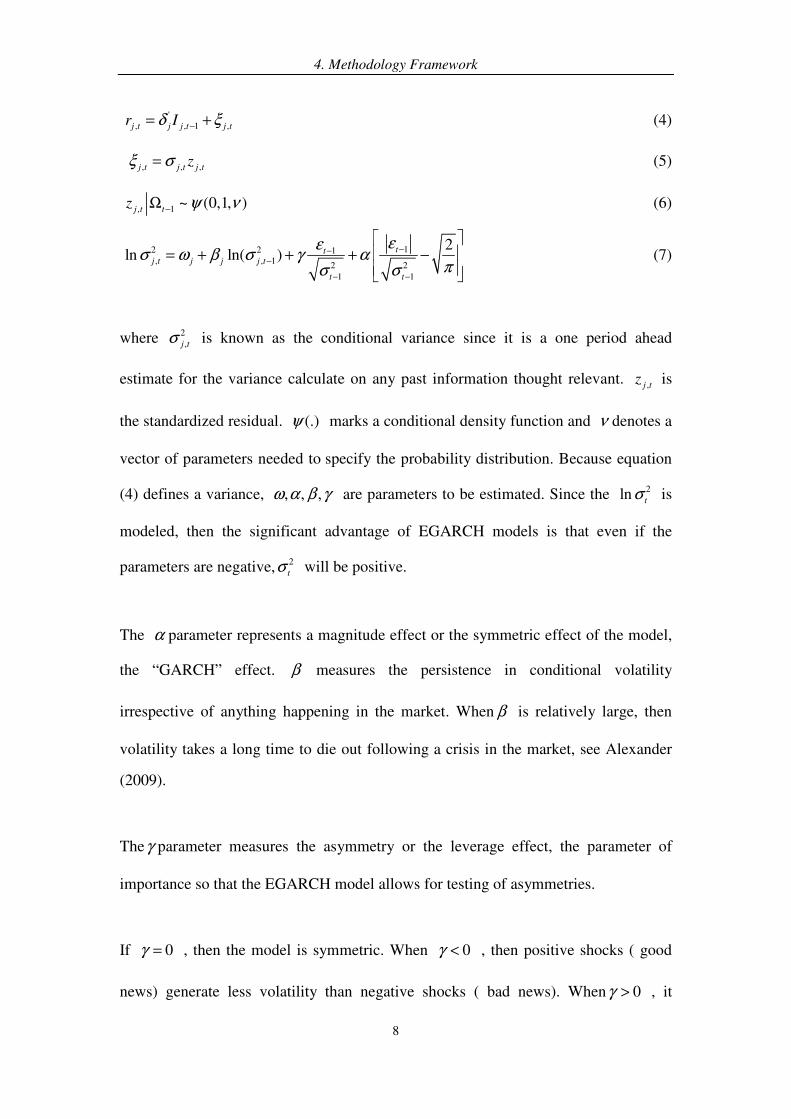
4.2 Extensions to the EGARCH model

Let ,j tr represents the return on a market index at time t, where subscript j∈

Shanghai A-shares, Shanghai B-shares, Shenzhen A-shares, Shenzhen B-shares,

Hang Seng, H- shares:


8

'

, , 1 ,j t j j t j tr Iδ ξ−= + (4)

, , ,j t j t j tzξ σ= (5)

, 1 ~ (0,1, )j t t

z ψ ν−Ω (6)

12 2 1, , 1

2 2

1 1

2ln ln( )

ttj t j j j t

t t

εεσ ω β σ γ α

πσ σ

−−−

− −

= + + + −

(7)

where 2

,j tσ is known as the conditional variance since it is a one period ahead

estimate for the variance calculate on any past information thought relevant. ,j tz is

the standardized residual. (.)ψ marks a conditional density function and ν denotes a

vector of parameters needed to specify the probability distribution. Because equation

(4) defines a variance, , , ,ω α β γ are parameters to be estimated. Since the 2lnt

σ is

modeled, then the significant advantage of EGARCH models is that even if the

parameters are negative, 2

tσ will be positive.

The α parameter represents a magnitude effect or the symmetric effect of the model,

the “GARCH” effect. β measures the persistence in conditional volatility

irrespective of anything happening in the market. When β is relatively large, then

volatility takes a long time to die out following a crisis in the market, see Alexander

(2009).

Theγ parameter measures the asymmetry or the leverage effect, the parameter of

importance so that the EGARCH model allows for testing of asymmetries.

If 0γ = , then the model is symmetric. When 0γ < , then positive shocks ( good

news) generate less volatility than negative shocks ( bad news). When 0γ > , it


9

implies that positive innovations are more destabilizing than negative innovations.

Our EGARCH (1, 1) model got a distinctive feature, i.e., conditional variance was

modeled to capture the leverage effect of volatility.

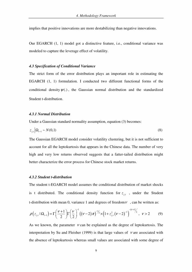
4.3 Specification of Conditional Variance

The strict form of the error distribution plays an important role in estimating the

EGARCH (1, 1) formulation. I conducted two different functional forms of the

conditional density (.)ψ , the Gaussian normal distribution and the standardized

Student t-distribution.

4.3.1 Normal Distribution

Under a Gaussian standard normality assumption, equation (3) becomes:

, 1 ~ (0,1)j t t

z N−Ω (8)

The Gaussian EGARCH model consider volatility clustering, but it is not sufficient to

account for all the leptokurtosis that appears in the Chinese data. The number of very

high and very low returns observed suggests that a fatter-tailed distribution might

better characterize the error process for Chinese stock market returns.

4.3.2 Student t-distribution

The student t-EGARCH model assumes the conditional distribution of market shocks

is t distributed. The conditional density function for ,j tz , under the Student

t-distribution with mean 0, variance 1 and degrees of freedomν , can be written as:

( ) ( )( ) ( )( )( )1 1

1 1 222, 1 ,

1| 2 1 2

2 2j t t j t

z z

νν ν

ρ ν π ν− − +

− −

−

+ Ω = Γ Γ − × + −

, 2ν > (9)

As we known, the parameter ν can be explained as the degree of leptokurtosis. The

interpretation by Su and Fleisher (1999) is that large values of ν are associated with

the absence of leptokurtosis whereas small values are associated with some degree of


10

leptokurtosis. If 1ν approaches 0, the Student t-distribution approaches to a

standard normal distribution, but when 1ν > 0, the t-distribution has fatter tails than

the corresponding normal distribution.

The normal EGARCH models (8) do not tend to fit financial returns in which the

market shocks have a non-normal conditional distribution. As above revealed, if

measured at the daily or higher frequency, market returns typically have skewed and

leptokurtic conditional (and unconditional) distributions, see Wang and Fawson,

(2001). The student-t EGARCH model, introduced by Bollerslev (1987), assumes the

conditional distribution of market shocks is t distributed. The degrees of freedom in

this distribution become an additional parameter that is estimated along with the

parameters in the conditional variance equation. The Student-t EGARCH model has

also been extended to skewed Student-t distributions by Lambert and Laurent (2001).

4.3 Long Term Volatility

According to Alexander (2009), without the market shocks the EGARCH variance

will ultimately settle down to a steady state value. This is the value 2

σ such that

22

tσ σ= for all t. We call

2

σ the unconditional variance of the EGARCH model.

The unconditional variance is the variance of the unconditional returns distribution,

which is assumed constant over the entire data period. It corresponds to a long term

average value of the conditional variance. The theoretical value of the EGARCH long

term or unconditional variance is not the same as the unconditional variance in a

moving average volatility model. The theoretical value of the unconditional variance

in an EGARCH model differs depending on the GARCH model. The long term or

unconditional variance is formatted by substituting 22 2

1t tσ σ σ−= = into the

EGARCH conditional variance equation. For example, for the EGARCH we use the

fact that 2 2

1 1( )t t

E ε σ− −= and then put 22 2

1t tσ σ σ−= = into (8) to obtain


11

2

exp1

ωσ

β

=

− (10)

The unconditional volatility (also called long term volatility) of the EGARCH (1, 1)

model is the annualized square root of (10). If unconditional volatility is relatively

large then long term volatility in the market is relatively high.

First, I measured the GARCH (1, 1) model and EGARCH (1, 1) under two alternative

formulations of the error-generation process. Then, I computed two tests, the

likelihood ratio test statistic and log likelihood comparison to choose the best-fitted

model. Finally, I utilized the parameter estimation under the best-fitted model.

Consecutively, I applied the best-fitted model to calculate the impact of long term

volatility.

5. Data and Preliminary Results

12

5 Data and Preliminary Results

5.1 Data Characteristic

The analysis in this paper was based on the Hang Seng, H-shares, A- and B-shares

data from 31 December 1999 until 8 April 2010. I initially estimated stock market

volatility and returns to investors using data of daily Chinese stock market indices.

There series were taken from DataStream and each consist of T= 2215 observations in

the last decade. In order to have a benchmark for the results, the study related trading

in these shares to daily market indices representing more mature stock markets,

including indices of the Tokyo Stock Exchange (Nikkei 225), the New York Stock

Exchange (NYSE) and S&P Stock Exchange (SP 500 index).

The sample data was split into the periods before and during the period of financial

crisis of 2007-2010. The first subsample covered all trading days between 2000 and

2006. The day trading (4 January 2007) during the financial crisis was the start of the

financial crisis subsample.

Let 1log( ) log( )t t t

P P P−= − stood for the daily return of the indext

P . Table 1 presents

some sample distributional statistics for the stock market indices included in this

paper. Statistics consist of the daily sample mean returns, standard deviation,

minimum returns and maximum returns. I characterize the stock market return and

volatility pattern as follows: (1) Mean returns for A- and B- shares on Shanghai and

Shenzhen securities exchanges as well as H-shares are positive and apparently higher

than the Hang Seng, Nikkei 225, NYSE and SP500 indices, but the standard

deviations of these returns (or the volatility of returns) are also higher. This output is

meaningful, because China got rapid growth in the past ten years and it boosted the

Chinese stock exchange flourishing compared to the other countries. (2) Mean returns

on A-shares are lower than those on B-shares for both exchanges, nevertheless the

volatility of returns are also smaller. (3) Hang Seng index generates different mean


13

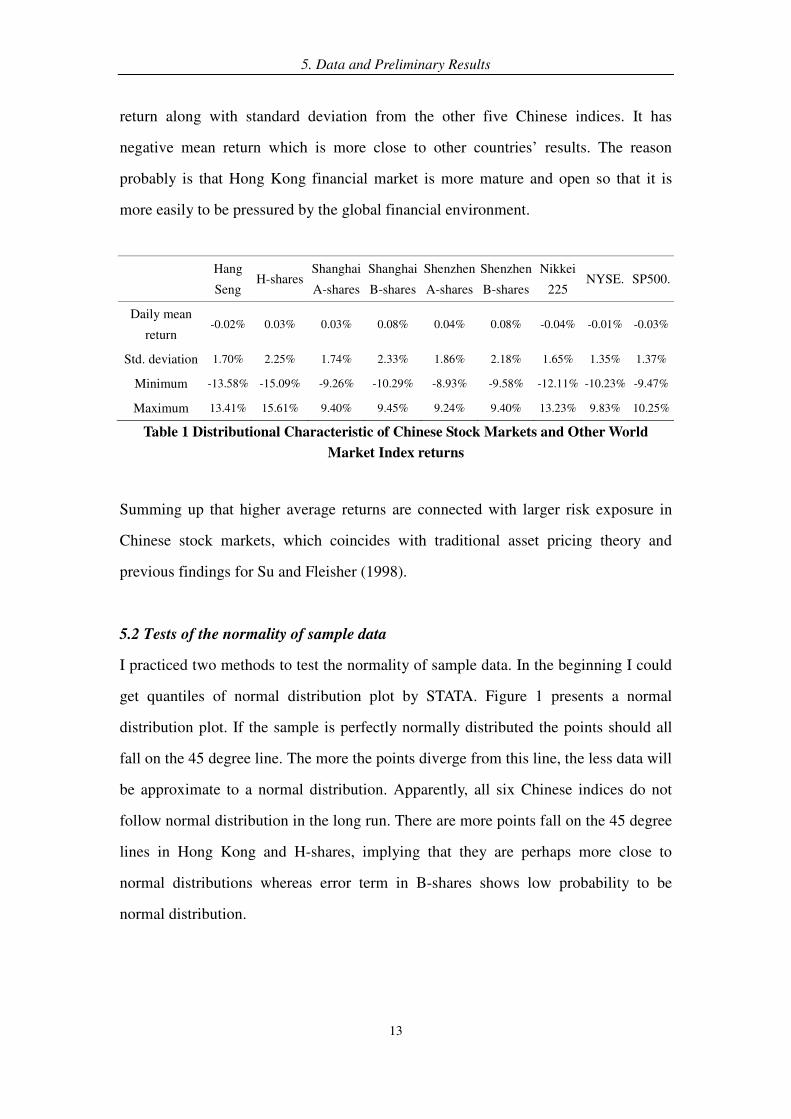
return along with standard deviation from the other five Chinese indices. It has

negative mean return which is more close to other countries’ results. The reason

probably is that Hong Kong financial market is more mature and open so that it is

more easily to be pressured by the global financial environment.

Hang

Seng H-shares

Shanghai

A-shares

Shanghai

B-shares

Shenzhen

A-shares

Shenzhen

B-shares

Nikkei

225 NYSE. SP500.

Daily mean

return -0.02% 0.03% 0.03% 0.08% 0.04% 0.08% -0.04% -0.01% -0.03%

Std. deviation 1.70% 2.25% 1.74% 2.33% 1.86% 2.18% 1.65% 1.35% 1.37%

Minimum -13.58% -15.09% -9.26% -10.29% -8.93% -9.58% -12.11% -10.23% -9.47%

Maximum 13.41% 15.61% 9.40% 9.45% 9.24% 9.40% 13.23% 9.83% 10.25%

Table 1 Distributional Characteristic of Chinese Stock Markets and Other World

Market Index returns

Summing up that higher average returns are connected with larger risk exposure in

Chinese stock markets, which coincides with traditional asset pricing theory and

previous findings for Su and Fleisher (1998).

5.2 Tests of the normality of sample data

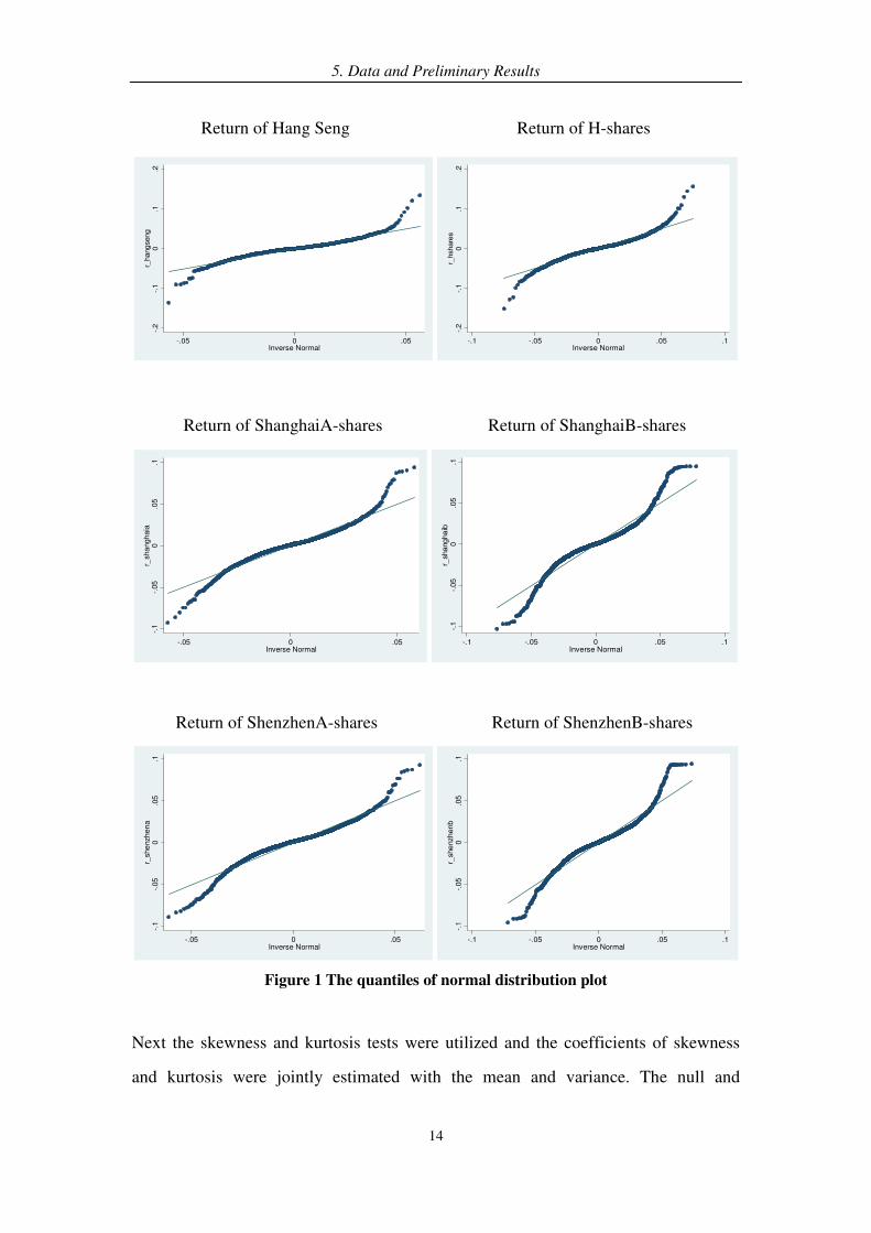
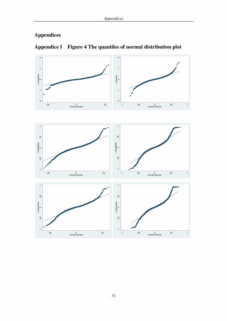
I practiced two methods to test the normality of sample data. In the beginning I could

get quantiles of normal distribution plot by STATA. Figure 1 presents a normal

distribution plot. If the sample is perfectly normally distributed the points should all

fall on the 45 degree line. The more the points diverge from this line, the less data will

be approximate to a normal distribution. Apparently, all six Chinese indices do not

follow normal distribution in the long run. There are more points fall on the 45 degree

lines in Hong Kong and H-shares, implying that they are perhaps more close to

normal distributions whereas error term in B-shares shows low probability to be

normal distribution.


14

Return of Hang Seng Return of H-shares

-.2

-.1

0.1

.2r_

hang

seng

-.05 0 .05Inverse Normal

-.2

-.1

0.1

.2r_

hshare

s

-.1 -.05 0 .05 .1Inverse Normal

Return of ShanghaiA-shares Return of ShanghaiB-shares

-.1

-.05

0.0

5.1

r_sha

ng

ha

ia


-.1

-.05

0.0

5.1

r_shangha

ib


Return of ShenzhenA-shares Return of ShenzhenB-shares

-.1

-.05

0.0

5.1

r_she

nzh

en

a


-.1

-.05

0.0

5.1

r_she

nzhenb


Figure 1 The quantiles of normal distribution plot

Next the skewness and kurtosis tests were utilized and the coefficients of skewness

and kurtosis were jointly estimated with the mean and variance. The null and


15

alternative hypothesis was that:

0H = The sample data are normally distributed

1H = 0H is not true

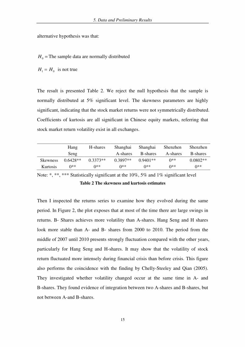
The result is presented Table 2. We reject the null hypothesis that the sample is

normally distributed at 5% significant level. The skewness parameters are highly

significant, indicating that the stock market returns were not symmetrically distributed.

Coefficients of kurtosis are all significant in Chinese equity markets, referring that

stock market return volatility exist in all exchanges.

Hang H-shares Shanghai Shanghai Shenzhen Shenzhen Seng A-shares B-shares A-shares B-shares

Skewness 0.6428** 0.3373** 0.3897** 0.9401** 0** 0.0802**

Kurtosis 0** 0** 0** 0** 0** 0**

Note: *, **, *** Statistically significant at the 10%, 5% and 1% significant level

Table 2 The skewness and kurtosis estimates

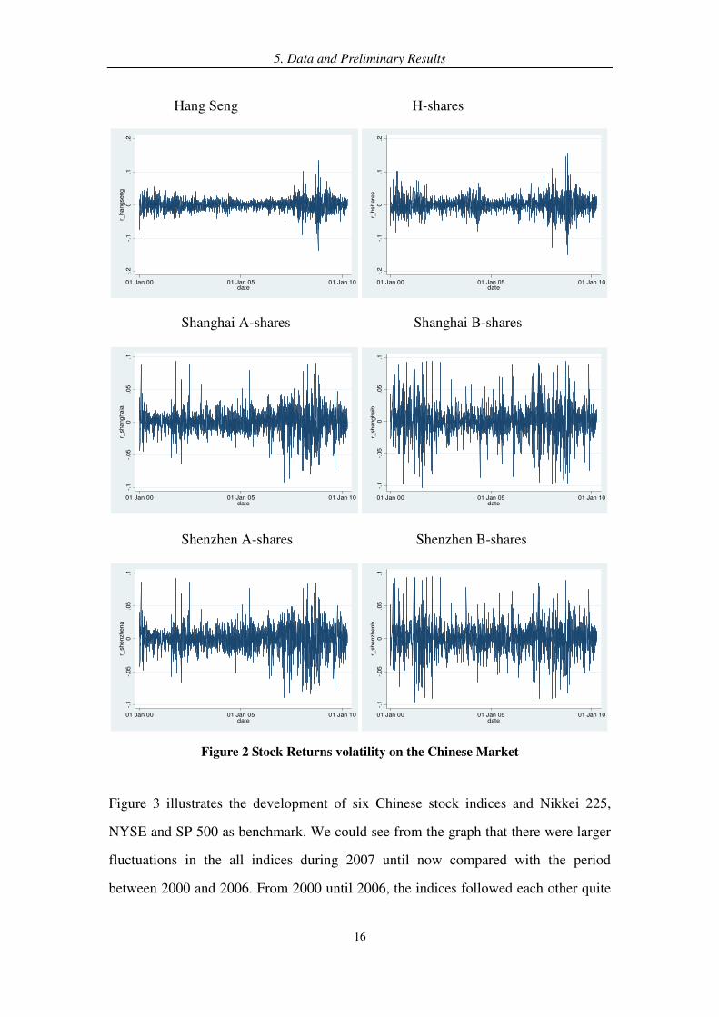
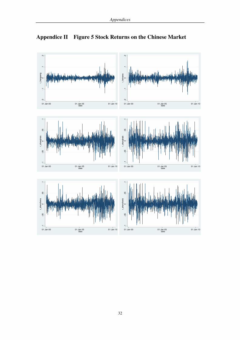
Then I inspected the returns series to examine how they evolved during the same

period. In Figure 2, the plot exposes that at most of the time there are large swings in

returns. B- Shares achieves more volatility than A-shares. Hang Seng and H shares

look more stable than A- and B- shares from 2000 to 2010. The period from the

middle of 2007 until 2010 presents strongly fluctuation compared with the other years,

particularly for Hang Seng and H-shares. It may show that the volatility of stock

return fluctuated more intensely during financial crisis than before crisis. This figure

also performs the coincidence with the finding by Chelly-Steeley and Qian (2005).

They investigated whether volatility changed occur at the same time in A- and

B-shares. They found evidence of integration between two A-shares and B-shares, but

not between A-and B-shares.


16

Hang Seng H-shares

-.2

-.1

0.1

.2r_

hangseng

01 Jan 00 01 Jan 05 01 Jan 10date

-.2

-.1

0.1

.2r_

hsh

are

s

01 Jan 00 01 Jan 05 01 Jan 10date

Shanghai A-shares Shanghai B-shares

-.1

-.05

0.0

5.1

r_shanghaia

01 Jan 00 01 Jan 05 01 Jan 10date

-.1

-.05

0.0

5.1

r_shanghaib

01 Jan 00 01 Jan 05 01 Jan 10date

Shenzhen A-shares Shenzhen B-shares

-.1

-.05

0.0

5.1

r_shenzhena

01 Jan 00 01 Jan 05 01 Jan 10date

-.1

-.05

0.0

5.1

r_shenzhen

b

01 Jan 00 01 Jan 05 01 Jan 10date

Figure 2 Stock Returns volatility on the Chinese Market

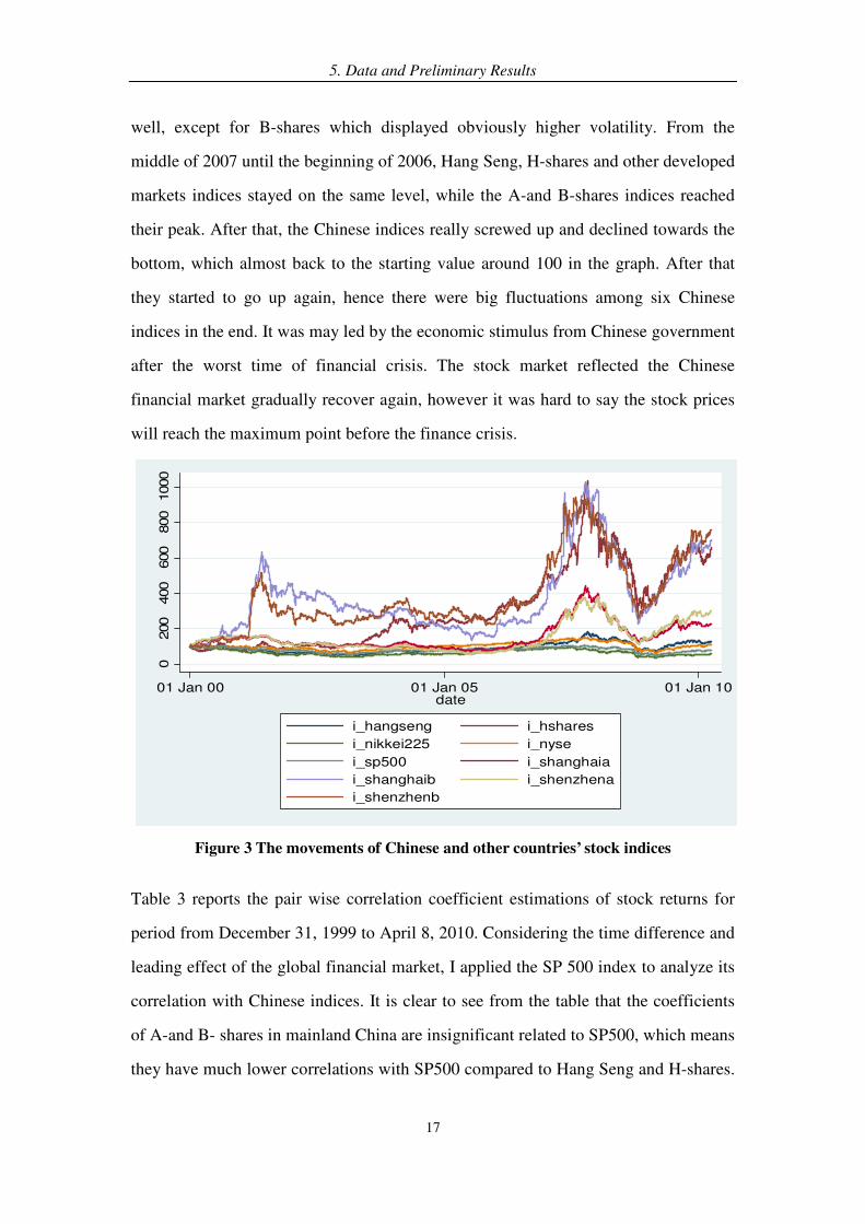
Figure 3 illustrates the development of six Chinese stock indices and Nikkei 225,

NYSE and SP 500 as benchmark. We could see from the graph that there were larger

fluctuations in the all indices during 2007 until now compared with the period

between 2000 and 2006. From 2000 until 2006, the indices followed each other quite


17

well, except for B-shares which displayed obviously higher volatility. From the

middle of 2007 until the beginning of 2006, Hang Seng, H-shares and other developed

markets indices stayed on the same level, while the A-and B-shares indices reached

their peak. After that, the Chinese indices really screwed up and declined towards the

bottom, which almost back to the starting value around 100 in the graph. After that

they started to go up again, hence there were big fluctuations among six Chinese

indices in the end. It was may led by the economic stimulus from Chinese government

after the worst time of financial crisis. The stock market reflected the Chinese

financial market gradually recover again, however it was hard to say the stock prices

will reach the maximum point before the finance crisis.

0200

400

600

800

1000

01 Jan 00 01 Jan 05 01 Jan 10date

i_hangseng i_hshares

i_nikkei225 i_nyse

i_sp500 i_shanghaia

i_shanghaib i_shenzhena

i_shenzhenb

Figure 3 The movements of Chinese and other countries’ stock indices

Table 3 reports the pair wise correlation coefficient estimations of stock returns for

period from December 31, 1999 to April 8, 2010. Considering the time difference and

leading effect of the global financial market, I applied the SP 500 index to analyze its

correlation with Chinese indices. It is clear to see from the table that the coefficients

of A-and B- shares in mainland China are insignificant related to SP500, which means

they have much lower correlations with SP500 compared to Hang Seng and H-shares.


18

But there is strong evidence of highly positive correlation between Shanghai and

Shenzhen A-and B-shares. This indicates that the stock markets in mainland China are

still a relatively separated market with other markets in the world during this period.

Hans Seng and H-shares get positive correlation with SP 500 index, although the

correlation between Hang Seng and SP 500 is higher than the correlation between

H-shares and SP 500. In view of the acceleration of openness for China’s capital

markets in recent years and financial crisis probably brought out specific effects, we

also presented the estimation results for the correlation coefficient from Jan.1, 2007 to

Apr. 8, 2010.

ShanghaiA ShanghaiB ShenzhenA ShenzhenB HangSeng H-shares SP500

ShanghaiA 1.0000

ShanghaiB 0.7323** 1.0000

ShenzhenA 0.9431** 0.7463** 1.0000

ShenzhenB 0.7237** 0.8527** 0.7256** 1.0000

HangSeng 0.3313** 0.2839** 0.2835** 0.3213** 1.0000

H-shares 0.3757** 0.3115** 0.3196** 0.3367** 0.7864** 1.0000

SP500 0.0186 0.0109 0.0075 0.0226 0.1845** 0.1455** 1.0000

Note: *, **, *** Statistically significant at the 10%, 5% and 1% significant level.

Table 3 Correlations between Different Markets for period 2000-2010

Table 4 displays the correlations between different markets for period 2007-2010. It is

interesting to see from the table that all coefficients between Chinese stock markets

are significant whereas only stock indices from Hong Kong have correlation with

SP500. It have a remarkable growing for the correlation between Hang Seng,

H-shares and SP 500 indices, inferring that the correlation of the global financial

infrastructure is steadily increasing. The correlation between Hang Seng and two

mainland stock markets is almost doubled, which means that Hong Kong stock

market become more integrated with the two mainland stock markets in recent years,

and we believe the trend should continue in the future, considering the closer and

closer economic relations between these market.

6. Empirical Results

19

ShanghaiA ShanghaiB ShenzhenA ShenzhenB HangSeng H-shares SP500

ShanghaiA 1.0000

ShanghaiB 0.8131** 1.0000

ShenzhenA 0.9266** 0.8353** 1.0000

shenzhenB 0.8263** 0.8942** 0.8279** 1.0000

HangSeng 0.4823** 0.4192** 0.4050** 0.4931** 1.0000

H-shares 0.5299** 0.4591** 0.4391** 0.5347** 0.9584** 1.0000

SP500 0.0523 0.0451 0.0348 0.0535 0.2643** 0.2440** 1.0000

Note: *, **, *** Statistically significant at the 10%, 5% and 1% significant level.

Table 4 Correlations between Different Markets for period 2007-2010

6 Empirical Results

6.1 Model Comparison

I conducted comparative tests of the models against conventional models presented in

this section. The criteria used to determine the performance include the log likelihood

value comparison and likelihood ratio test according to Alexander (2009).

Since the prevailing concern about traditional GARCH models of stock index returns

was their unsatisfactory accommodation of the leverage effect, volatility persistence,

fat tails and skewness, I proposed an EGARCH model to accommodate these

characteristics. The skewness and kurtosis test in the last section in the standardized

residuals indicated the inappropriateness of the assumption of conditional normality in

the error distribution.

This model structure was tested against GARCH models using Gaussian and student-t

distribution assumptions. In all, four models were estimated: Gaussian GARCH and

Gaussian EGARCH, student-t GARCH and student-t EGARCH.

I chose among the alternative error-distribution formulations for the best fit by first

comparing the log likelihood Value and likelihood ratio statistics would be applied for


20

six Chinese stock indices.

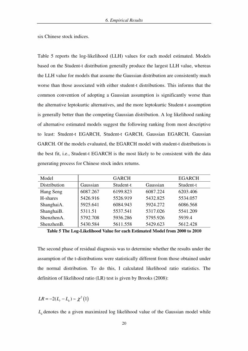
Table 5 reports the log-likelihood (LLH) values for each model estimated. Models

based on the Student-t distribution generally produce the largest LLH value, whereas

the LLH value for models that assume the Gaussian distribution are consistently much

worse than those associated with either student-t distributions. This informs that the

common convention of adopting a Gaussian assumption is significantly worse than

the alternative leptokurtic alternatives, and the more leptokurtic Student-t assumption

is generally better than the competing Gaussian distribution. A log likelihood ranking

of alternative estimated models suggest the following ranking from most descriptive

to least: Student-t EGARCH, Student-t GARCH, Gaussian EGARCH, Gaussian

GARCH. Of the models evaluated, the EGARCH model with student-t distributions is

the best fit, i.e., Student-t EGARCH is the most likely to be consistent with the data

generating process for Chinese stock index returns.

Model GARCH EGARCH

Distribution Gaussian Student-t Gaussian Student-t

Hang Seng 6087.267 6199.823 6087.224 6203.406

H-shares 5426.916 5526.919 5432.825 5534.057

ShanghaiA. 5925.641 6084.943 5924.272 6086.568

ShanghaiB. 5311.51 5537.541 5317.026 5541.209

ShenzhenA. 5792.708 5936.286 5795.926 5939.4

ShenzhenB. 5430.584 5611.558 5429.623 5612.428

Table 5 The Log-Likelihood Value for each Estimated Model from 2000 to 2010

The second phase of residual diagnosis was to determine whether the results under the

assumption of the t-distributions were statistically different from those obtained under

the normal distribution. To do this, I calculated likelihood ratio statistics. The

definition of likelihood ratio (LR) test is given by Brooks (2008):

( )22( ) ~ 1r uLR L L χ= − −

uL denotes the a given maximized log likelihood value of the Gaussian model while


21

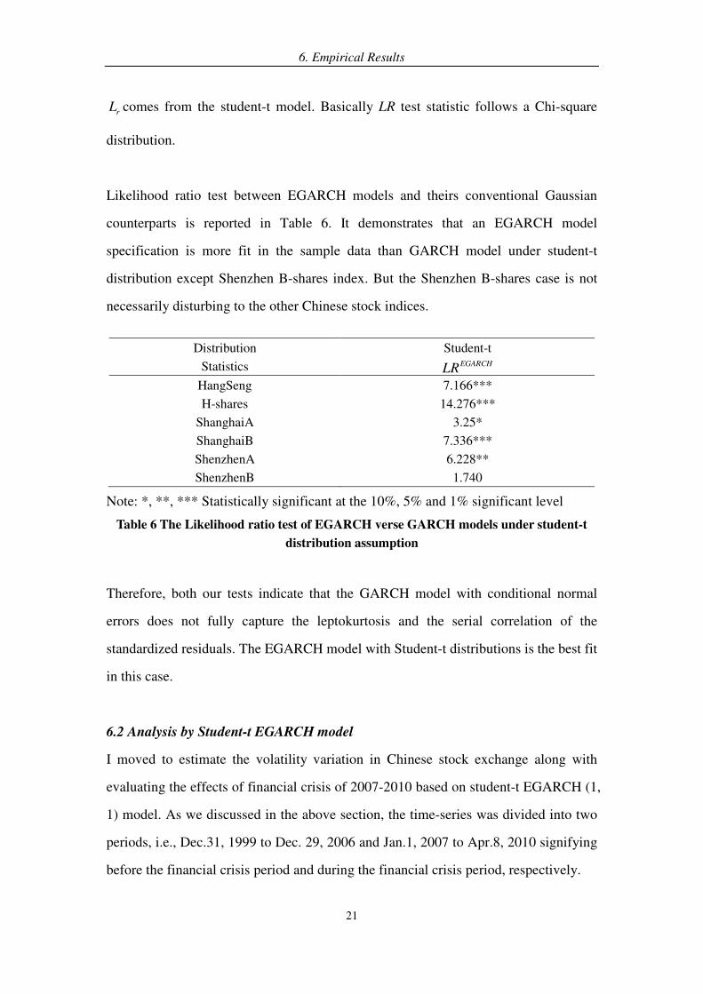
rL comes from the student-t model. Basically LR test statistic follows a Chi-square

distribution.

Likelihood ratio test between EGARCH models and theirs conventional Gaussian

counterparts is reported in Table 6. It demonstrates that an EGARCH model

specification is more fit in the sample data than GARCH model under student-t

distribution except Shenzhen B-shares index. But the Shenzhen B-shares case is not

necessarily disturbing to the other Chinese stock indices.

Distribution Student-t

Statistics EGARCHLR

HangSeng 7.166***

H-shares 14.276***

ShanghaiA 3.25*

ShanghaiB 7.336***

ShenzhenA 6.228**

ShenzhenB 1.740


Table 6 The Likelihood ratio test of EGARCH verse GARCH models under student-t

distribution assumption

Therefore, both our tests indicate that the GARCH model with conditional normal

errors does not fully capture the leptokurtosis and the serial correlation of the

standardized residuals. The EGARCH model with Student-t distributions is the best fit

in this case.

6.2 Analysis by Student-t EGARCH model

I moved to estimate the volatility variation in Chinese stock exchange along with

evaluating the effects of financial crisis of 2007-2010 based on student-t EGARCH (1,

1) model. As we discussed in the above section, the time-series was divided into two

periods, i.e., Dec.31, 1999 to Dec. 29, 2006 and Jan.1, 2007 to Apr.8, 2010 signifying

before the financial crisis period and during the financial crisis period, respectively.


22

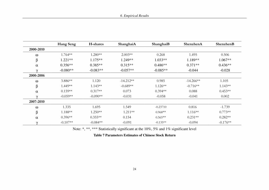
The parameter estimation for the EGARCH (1, 1) model is presented in Table 7.

According to the results we can find that the leverage effects γ are almost negative

that significant at 5% significant level which means that good news generates less

volatility than bad news for Chinese stock market despite of financial crisis2. It is

interesting to observe that the coefficient of Shenzhen B-shares before financial crisis

is positive as the exception. The possible reason is that because B-shares market is

quite young financial market, it have special characteristic and does not follow any

track of movement. Nevertheless, by developing several years later, the leverage

effect of Shenzhen B-shares exhibits the similar output as the other Chinese stock

markets. Furthermore, during the financial crisis γ is larger than it compares with

the period before the crisis and also there are more γ are significant during the crisis

period. Thus we might be able to say that investors of Chinese stock market preferred

to hear good news than bad news when they suffer the bad time. Basically in the crisis,

shareholders feel scarier for bad news, because bad investment will go bankrupt. It is

reliable to declare that stock market is more sensitive for bad news.

To all indices during financial crisis, the symmetric effect α which is a little bit

different than it in the previous period in EGARCH model, however it is relatively

large than 0.1 too, so it means that the volatility is sensitive to market events in the

whole period. On the other hand, during the crisis α is the largest, implying that

volatility was very sensitive in the bad time.

The parameter β measures the persistence in conditional volatility irrespective of

anything happening in the market. Besides the parameter of A-shares before the crisis,

β are all positive and relatively large, e.g. above 0.9, then volatility taks long time to

2 See page 8.


23

die out following a crisis in the Chinese stock market.

Also, according to the relative scale of the coefficients, the leverage effect or the

symmetric effects dominated. In order to find the long term volatility, we first have to

find the long term variance in the EGARCH model.


24

Hang Seng H-shares ShanghaiA ShanghaiB ShenzhenA ShenzhenB

2000-2010

ω 1.764** 1.280** 2.003** 0.268 1.495 0.506

β 1.221** 1.175** 1.249** 1.033** 1.189** 1.067**

α 0.356** 0.385** 0.315** 0.486** 0.371** 0.436**

γ -0.080** -0.083** -0.057** -0.085** -0.044 -0.028

2000-2006

ω 3.886** 1.120 -14.212** 0.985 -14.266** 1.105

β 1.449** 1.143** -0.689** 1.126** -0.716** 1.143**

α 0.159** 0.317** 0.073 0.394** 0.088 0.453**

γ -0.059** -0.090** -0.031 -0.058 -0.041 0.002

2007-2010

ω 1.335 1.695 1.549 -0.23710 0.816 -1.739

β 1.188** 1.250** 1.211** 0.968** 1.116** 0.773**

α 0.396** 0.355** 0.154 0.565** 0.231** 0.282**

γ -0.107** -0.084** -0.091 -0.135** -0.094 -0.176**


Table 7 Parameters Estimates of Chinese Stock Return

7. Summary and Conclusion

25

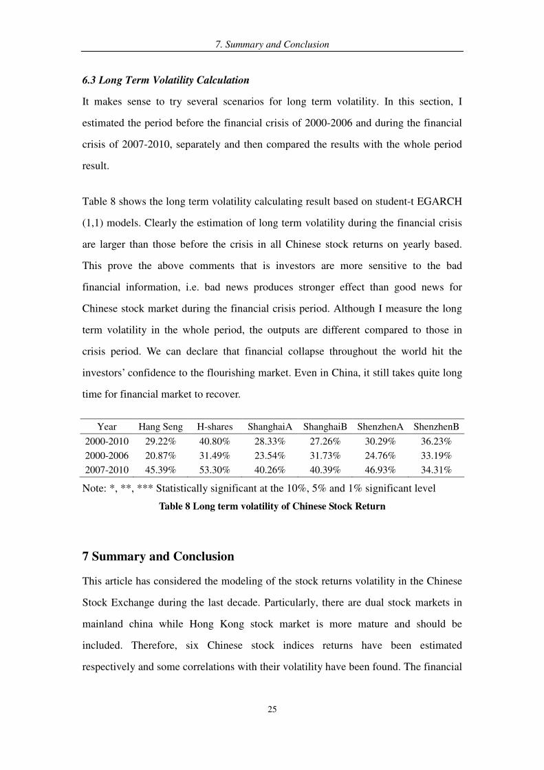
6.3 Long Term Volatility Calculation

It makes sense to try several scenarios for long term volatility. In this section, I

estimated the period before the financial crisis of 2000-2006 and during the financial

crisis of 2007-2010, separately and then compared the results with the whole period

result.

Table 8 shows the long term volatility calculating result based on student-t EGARCH

(1,1) models. Clearly the estimation of long term volatility during the financial crisis

are larger than those before the crisis in all Chinese stock returns on yearly based.

This prove the above comments that is investors are more sensitive to the bad

financial information, i.e. bad news produces stronger effect than good news for

Chinese stock market during the financial crisis period. Although I measure the long

term volatility in the whole period, the outputs are different compared to those in

crisis period. We can declare that financial collapse throughout the world hit the

investors’ confidence to the flourishing market. Even in China, it still takes quite long

time for financial market to recover.

Year Hang Seng H-shares ShanghaiA ShanghaiB ShenzhenA ShenzhenB

2000-2010 29.22% 40.80% 28.33% 27.26% 30.29% 36.23%

2000-2006 20.87% 31.49% 23.54% 31.73% 24.76% 33.19%

2007-2010 45.39% 53.30% 40.26% 40.39% 46.93% 34.31%


Table 8 Long term volatility of Chinese Stock Return

7 Summary and Conclusion

This article has considered the modeling of the stock returns volatility in the Chinese

Stock Exchange during the last decade. Particularly, there are dual stock markets in

mainland china while Hong Kong stock market is more mature and should be

included. Therefore, six Chinese stock indices returns have been estimated

respectively and some correlations with their volatility have been found. The financial


26

crisis attracts us to evaluate its effect to Chinese stock market so that we can use daily

data for the periods before and during financial crisis.

Stock index return data for Chinese stock market have been examined to compare the

performance of GARCH and EGARCH models under two distributional assumptions:

Gaussian, student-t distributions. There are enough evidences to reject the

assumptions of conditional normality in a broad cross-section of Chinese stock index

data series: this reflected in the form of skewness and kurtosis. Although traditional

GARCH modeling with a leptokurtic distribution have been found which is useful to

account for the conditional heteroscedasticity and leptokurtosis, it cannot easily

accommodate other commonly observed stylized characteristics in our sample data,

such as skewness.

In addition, the evidences of leverage effect and volatility persistence are well

documented in the literature for Chinese stock market estimations. The results

indicate that it is important to specify the EGARCH model which is sufficiently

flexible to accommodate these data characteristics because estimation procedures that

fail to explicitly account for data characteristics are likely to lead to spurious results.

As expected before, I have found that the most empirical evidence favors EGARCH

models which allow for the increased flexibility provided by the student-t

specification. Empirical evidences suggest that the EGARCH model provides a better

description and more parsimonious representation than the traditional GARCH model.

Since the EGARCH model with student-t distribution outperform better than normal

GARCH model, I apply it to estimate the parameters together with three time periods,

i.e, the whole period, before the financial crisis and during the crisis. The finding is

that Chinese stock market is dramatically beat by the financial crisis and it takes a

long time for investors to recover their confidence to market. On the other hand, the

result also shows that the stimulus policies by Chinese government lead the price of


27

stock increase again. It is a good sign for Chinese financial market to boom in the

future.

Reference

28

Reference

1. Literature

1.1 Books

Chris Brooks. (2008) “Introductory Econometrics for Finance”, Cambridge University

Press.

Carol Alexander. (2009) “Practical Financial Econometrics”, John Wiley & Sons, Ltd.

1.2 Journal articles

Taufiq Choudhry. (1996) “Stock market volatility and the crash of 1987: evidence

from six emerging market”, Journal of International Money and Finance Vol.15, and

No.6:996-981

Chou,Ray.(1988) “ Volatility persistence and stock valuation: Some empirical

evidence using GARCH”, Review of Economics and Statistics June, 69:542-547

Baillie, Richard and Ramon Degennaro. (1990) “Stock returns and volatility”, Journal

of Financial and Quantitative Analysis June, 25:203-214

Alexander C,Lazar E.(2004) “ The equity index skew, market crashes and asymmetric

normal mixture GARCH. ISMA Center Discussion Papers in Finance 2004-14

Anastassios A. Drakos, Georgios P. Kouretas and Leonidas P. Zarangas. (2010)

“Forcasting financial volatility of the Athens Stock Exchange daily returns: An

application of the asymmetric normal mixture GARCH model”, International Journal

of Finance and Economics: 1-4.

Y.Gao and Y.K.Tse. (2004) “Capital control, market segmentation and cross-border

flow of information: Some empirical evidence from the Chinese stock market”,

International Review of Economics & Finance Vol.13, No.4

Reference

29

Steven Shuye Wang, Li Jiang. (2004) “Location of trade, ownership restrictions, and

market illiquidity: Examinging Chinese A-and H-shares”, Journal of Banking &

Finance 28: 1273-1297.

Jiangyu Wang. (2004) “Dancing with wolves: Regulation and Deregulation of Foreign

Investment in China’s Stock Market”, Asian-Pacific Law & Policy Journal Vol.5:1-61

Niklas Ahlgren, Bo Sjo and Jianhua Zhang. (2009) “Panel cointegration of Chinese A

and B shares”, Applied Financial Econometric 19:1857-1871.

Kim, Y. and Shin, J. (2000) “Interactions among China related stocks”, Asia-Pacific

Financial Markets, 7:97-115.

Chelly-Steeley, P. and Qian, W. (2005) “Testing for market segmentation in the A and

B share markets of China”, Applied Financial Econometric15: 791-802.

Kai-Li Wang and Christopher Fawson.(2001) “Modeling Asian Stock Returns with a

More General Parametric GARCH Specification”, Journal of Financial Studies Vol.9

No.3 December: 21-52.

Alexander C, Lazar E. (2006) “Normal mixture GARCH (1, 1): application to

exchange rate modeling”, Journal of Applied Econometrics Economic Review

39:885-905

Dongwi Su and Belton M. Fleisher. (1998) “Risk, Return and Regulation in Chinese

Stock Market”, Journal of Econometric and Business 50: 239-256.

Lambert P, Laurent S. (2001) “Modeling financial time series using

Reference

30

GARCH-typemodels with a skewed Student distribution for the innovations”,

Working Paper, University de Liege

Chelly-Steeley,P. and Qian,W. (2005) “ Testing for market segmentation in the A and

B share markets of China”, Applied Financial Economics,15:791-802

2. Internet

China Securities Regulatory Commission, http://www.csrc.gov.cn/pub/newsite/

National Bereau of Statistics of China, http://www.stats.gov.cn/

Hang Seng Indexes http://www.hsi.com.hk

Martin T. Bohl, Michael Schuppli and Pierre L.Siklos, (2009) “Stock return

seasonalities and investor structure: Evidence from China’s B-share markets”, BOFIT

Discussion Papers, Electronic copy available at : http://ssrn.com/abstract=1496338

Appendices

31

Appendices

Appendice I Figure 4 The quantiles of normal distribution plot

-.2

-.1

0.1

.2r_

ha

ng

se

ng


-.2

-.1

0.1

.2r_

hsh

are

s


-.1

-.05

0.0

5.1

r_sha

ng

ha

ia


-.1

-.05

0.0

5.1

r_shangha

ib


-.1

-.05

0.0

5.1

r_she

nzh

en

a


-.1

-.05

0.0

5.1

r_sh

enzh

en

b


Appendices

32

Appendice II Figure 5 Stock Returns on the Chinese Market

-.

2-.

10

.1.2

r_ha

ngseng

01 Jan 00 01 Jan 05 01 Jan 10date

-.2

-.1

0.1

.2r_

hsh

are

s

01 Jan 00 01 Jan 05 01 Jan 10date

-.1

-.05

0.0

5.1

r_shanghaia

01 Jan 00 01 Jan 05 01 Jan 10date

-.1

-.05

0.0

5.1

r_shanghaib

01 Jan 00 01 Jan 05 01 Jan 10date

-.1

-.05

0.0

5.1

r_shenzhen

a

01 Jan 00 01 Jan 05 01 Jan 10date

-.1

-.05

0.0

5.1

r_shenzhen

b

01 Jan 00 01 Jan 05 01 Jan 10date

Documents

Application of EGARCH Model to Estimate Financial ... · Abstract i Application of EGARCH model to estimate financial volatility of daily returns: The empirical case of China Chang