Application of SWAP-WOFOST to evaluate the influence of water

and oxygen stress on potato yield in a Dutch farm

MSc. Thesis

PPS-80436

Plant Production Systems

Wageningen University

By:

Yulin Yan

Supervisors:

Pytrik Reidsma

Joop Kroes

April 2015

2

List of Important Acronyms

AMAXTB maximum leaf CO2 assimilation rate as a function of development stage of the crop

DM dry matter

DVS development stages

EF model efficiency

FLTB assimilates partitioning factors: fraction leaves

FM fresh matter

FOTB assimilates partitioning factors: fraction organs

FSTB assimilates partitioning factors: fraction stems

OB observation

SLATB specific leaf area

SM simulation

SPAN life span of leaves

SSE sum of squared errors

SWAP Soil Water Atmosphere Plant

TSUM1 the temperature sum from emergence to anthesis

TSUM2 the temperature sum from anthesis to maturity

TSUMEM temperature sum from sowing to emergence

TWSO total dry weight of storage organs

UWW under water tuber weight

WOFOST WOrld FOod Studies

WSO dry matter weight of storage organ

Ya actual yield

Yn nutrient-limited yield

Yp potential yield

Yw water-limited yield

3

Acknowledgements

I want to thank my supervisors: Pytrik Reidsma and Joop Kroes. Thanks for guiding me for my thesis

and giving helpful feedbacks to improve my thesis study. I would like to thank Pytrik Reidsma for

introducing the modelling approach and systems analysis to me and taking me to the farm. I would

like to thank Joop Kroes for helping me to learn SWAP and searching data.

I would also like to thank Jacob van den Borne and Wilko van der Velde for providing me data to do

this study. Moreover, I want to thank Joost Wolf , Jarno Rietema and João Nunes Vieira da Silva for

helping me during the study.

Furthermore, I want to thank my family for supporting me to study in Wageningen.

Finally, I want to thank my boyfriend who did not show up in the first 24 years of my life, which

allowed me to fully concentrate on my study.

4

Abstract

Potato (Solanum tuberosum L.) is one of the most important food crops in the world and it is

sensitive to water stress. The purpose of this study was to investigate the influence of drought and

oxygen stress on potato yields in the south of the Netherlands and improve water management at

farm level.

Yield gap analysis was done by using the integrated agro-hydrology and crop growth model SWAP-

WOFOST. The model WOFOST was calibrated at the potential production level before integration

with SWAP. The integrated model SWAP-WOFOST was not calibrated but applied using standard

parameters, but sensitivity analysis were performed to assess uncertainty of estimated water-limited

yields.

WOFOST was well calibrated with satisfactory validation results, with a model efficiency between

0.89-0.95 for (4 out of 5) fields in terms of fresh matter tuber yield simulation. Potential fresh yield of

potato cultivar Fontane was determined at the farm with a range of 90-120 t/ha, depending on the

growing period and weather (e.g. radiation, temperature). Simulated yield gap (FM) caused by water

was 18.7 to 31.0 t/ha in 2013 and 0.6-10.7 t/ha in 2014. Yield gap caused by water in 2013 & 2014

was mainly due to water deficiency. Moreover, it was found that tuber yield largely reduced by the

insufficient water supply at the tuber initiation and filling stages (MacKerron and Jefferies, 1986;

Haverkort et al., 1990; Lynch et al., 1995; Yuan et al., 2003). Oxygen stress was also found at some

fields with the insignificant impact on the yield. In 2013, drought stress was found strongly

influenced by the precipitation, soil characteristics and also ground water levels in the model

simulations. Therefore, precise precipitation data, soil inputs data and groundwater level data are

both essential for robust model results. Furthermore, SWAP-WOFOST was served to qualitatively

plan irrigation schedules to close water limited yield gaps. The complete and accurate data (rainfall,

soil, groundwater) are required in order to implement the model for irrigation schedule.

However, actual tuber yield were found even larger than simulated potential yield at some fields in

2014. This can be attributed to the yield data selection during the calibration. This issue can be

solved with experiments under potential production conditions. As for SWAP-WOFOST performance,

the water limited yield simulations cannot be verified because no water limited production

experiments were done at the farm. Yield gaps caused by drought and oxygen stress cannot be

exactly determined, as improved calibration is needed, but is clear that a large part of yield gaps can

be explained by water limitation during the growing season. Further experiments are required for

SWAP-WOFOST calibration.

5

Contents 1. Introduction ..................................................................................................................................... 7

1.1 Problem statement .................................................................................................................... 7

1.1.1 Growing food demand............................................................................................................ 7

1.1.2 Yield gap analysis .................................................................................................................... 7

1.1.3 Yield gap analysis on a precision agriculture farm ................................................................. 8

1.1.4 Drought stress ........................................................................................................................ 8

1.1.5 Oxygen stress.......................................................................................................................... 9

2. Research Aim & Questions ............................................................................................................ 11

2.1 Research Aim ........................................................................................................................... 11

2.2 Research Questions ................................................................................................................. 11

3 Materials and Methods .................................................................................................................. 13

3.1 Case Study and data ................................................................................................................ 13

3.1.1 Van den Borne Aardappelen ................................................................................................ 13

3.1.2 Climate .................................................................................................................................. 13

3.1.3 Soil information .................................................................................................................... 15

3.2 Structure of WOFOST .............................................................................................................. 16

3.2.1 Phenological development ................................................................................................... 17

3.2.2 Light interception and assimilation ...................................................................................... 17

3.3 Structure of SWAP ................................................................................................................... 19

3.3.1 Soil water flow and bottom boundary condition ................................................................. 19

3.3.2 Rainfall interception and evapotranspiration ...................................................................... 20

3.3.3 Water stress and oxygen stress ............................................................................................ 21

3.4 WOFOST Calibration for Potential Yield .................................................................................. 23

3.4.1 Fields and Data ..................................................................................................................... 23

3.4.2 Potential yield without calibration ....................................................................................... 24

3.4.3 Model Parameters ................................................................................................................ 24

3.4.4 Parameter sensitivity ............................................................................................................ 24

3.4.5 Calibration procedure........................................................................................................... 24

3.5 Potential yield validation ......................................................................................................... 25

3.6 Additional statistic methods .................................................................................................... 26

3.7 Drought & oxygen stress simulation ....................................................................................... 27

3.7.1 Drought stress sensitivity to precipitation and soil .............................................................. 28

3.7.2 Pressure head and ground water level................................................................................. 28

6

3.7.3 Irrigation scheduling ............................................................................................................. 29

4 Results ........................................................................................................................................ 31

4.1 Estimating potential yields without calibration ...................................................................... 31

4.2 Sensitivity analysis ................................................................................................................... 31

4.3 WOFOST calibration for potential yield simulation ................................................................. 32

4.3.1 TSUMEM calibration ............................................................................................................. 32

4.3.2 TSUM1 calibration ................................................................................................................ 33

4.3.4 TSUM2 calibration ................................................................................................................ 33

Fig. 22. Observed and simulated maturity with different TSUM2 values. .................................... 33

4.3.3 SPAN calibration ................................................................................................................... 33

4.3.5 AMAXTB calibration .............................................................................................................. 34

4.3.6 WOFOST validation ............................................................................................................... 37

4.4 Drought & oxygen stress simulation ....................................................................................... 38

4.4.1 Water limited yield without irrigation .................................................................................. 38

4.4.2 Sensitivity analysis of pressure head and underground water level ........................................ 39

4.4.4 The impact of rainfall and soil type on drought stress ......................................................... 42

4.4.5 Simulation with irrigation ..................................................................................................... 44

5. Discussion .................................................................................................................................. 47

5.1 WOFOST calibration and validation for potential yield simulation ......................................... 47

5.2 Water limited yield simulation ................................................................................................ 48

5.4 Implement SWAP-WOFOST for irrigation schedule ................................................................ 49

6. Conclusions & Recommendations ............................................................................................. 51

Reference ............................................................................................................................... 52

APPENDIX ...................................................................................................................................... 56

Appendix I ...................................................................................................................................... 56

Appendix II ..................................................................................................................................... 57

Appendix III .................................................................................................................................... 58

Appendix IV ................................................................................................................................... 58

Appendix V.................................................................................................................................... 59

Appendix VI................................................................................................................................... 59

Appendix VII .................................................................................................................................. 60

Appendix VIII ................................................................................................................................. 61

7

1. Introduction

1.1 Problem statement

1.1.1 Growing food demand

According to the UN (2013), a world population of 9.6 billion is expected in 2050. Thus, to satisfy

increasing food demands there is a great challenge to global crop production in the coming decades.

Generally (1) expanding agricultural land area and (2) increasing the yield are the two possible

approaches to increase production (Licker et al., 2010). However, due to the shortage of productive

land and growing demand of non-agricultural land uses, expanding agricultural area will not be the

desirable option. Therefore, increasing the yield will be the key to satisfy the future requirements

(Neumann et al., 2010). The Green Revolution that started in the middle of the 20th century, has led

to a high yield increase in many countries by introducing high-yielding crop varieties and artificial

fertilizers and pesticides (Hedden, 2003). However, in developed countries like the Netherlands this

led to environmental pollution, like nitrate leaching and biodiversity loss. And although yields in the

Netherlands are close to the optimal level (Van Ittersum et al., 2013), there is still a large variability

(spatial & temporal) and uncertainty among and within farms

(http://www.vandenborneaardappelen.com/).

1.1.2 Yield gap analysis

Yield gap analysis is applied to identify and sequence the influence of possible factors (e.g. water,

nutrient) on yield which can be the interpretive outcomes of the observed yield and it has been used

widely in many countries (Prost and Jeuffroy, 2008). In order to have a clear overview of yield gap

analysis, several basic concepts are introduced here. Potential yield (Yp) is defined as the yield of a

crop cultivar obtained when the crop is optimally supplied with water and nutrients and is

completely protected against growth-reducing factors. The potential yield is determined by the

weather (i.e. temperature, CO2, radiation) and crop properties (Van Ittersum and Rabbinge, 1997).

Definition of water-limited (Yw) and nutrient-limited (Yn) yield is related to Yp, but crop growth is

limited by water and nutrient supply respectively (Van Ittersum et al., 2013). Actual yield (Ya) is not

only influenced by growth-defining and growth-limiting factors but also affected by pests and

diseases and sub-optimal management (Fig. 1). The yield gap (Yg) is defined as the difference

between benchmark yield (could be Yp, Yw or Yn) and actual yield (Ya).

Yield can be increased by closing the yield gap (Van Ittersum et al., 2013). In the Netherlands,

potential yields are still linearly increasing due to genetic improvement of crops (Rijk et al., 2013).

Yield gaps vary widely across the globe (Neumann et al., 2010), but also among and within farms, as

mentioned above. In the Netherlands, the average yield gap is less than 20% (Van Ittersum et al.,

2013), but for individual farms and fields, large gaps occur. Moreover, most yield gap analysis focus

on the global and regional level. To better understand the impacts of farm characteristics, crop

management and soil conditions, it is important to study variations between and within farms.

However, yield gap analysis based on fields experiments are time consuming and expensive. Several

processed based crop models, integrating system approaches and multiple disciplines, have been

developed in the last decades which can assist yield gap analysis (Bhatia et al., 2008; Boote et al.,

1996). In this study, the model SWAP-WOFOST was used. Detailed information of the model SWAP-

WOFOST will be described in the methods section.

8

Fig. 1. Different production levels as determined by different factors respectively (Van Ittersum et al.,

2013)

1.1.3 Yield gap analysis on a precision agriculture farm

Precision agriculture is a production system that promotes variable management practices within a

field, according to site conditions. The system is based on the global positioning system (GPS),

geographic information systems (GIS), yield monitoring devices, soil, plant and pest sensors, remote

sensing and other technologies (Seelan et al., 2003). Van den Borne Aardappelen is a Dutch potato

farm located at the border of the Netherlands and Belgium. In 2007, Van den Borne started to

integrate precision agriculture into their business. By taking site specific conditions into account, the

application efficiency of fertilizer, pesticide, water and fossil fuel can be achieved optimally and at

the right time (http://precisielandbouw.eu/pplnl/Home.html). To improve the precision agriculture,

Van den Borne Aardappelen started another program called “Making Sense” in 2010 with BLGG ,

TTW (agricultural consultancy company) and WUR (Wageningen University and Research Centre).

The project Making Sense contributes to the development of a precision management decision

module for soil fertility and fertilization of arable crops on the basis of soil and crop sensor data,

climate data, a soil and a crop model (http://www.vandenborneaardappelen.com/.html). Within the

farm Van den Borne Aardappelen yield gaps vary. In order to make better use of the data collected in

the farm and improve farm management, a yield gap analysis is expected to be increase efficiency of

inputs for the fields within this farm.

1.1.4 Drought stress

Water is important for plant growth. It is the fundamental molecule for plant physiological activities.

Moreover potato has a high water content which accounts for approximately 85% of the composition

in living plant tissues. 1 % of the water is needed for metabolic processes and 99% for transpiration.

Water stress can cause severe physiological impacts, for instance on photosynthesis, transpiration

and cell development (Van Loon, 1981).

The potato crop is sensitive to water deficiency. Water stress could lead to reducing leaf area and/or

reducing photosynthesis efficiency at all stages of potato growth. Water shortage in the tuber filling

period causes most significant yield loss compared to drought during other stages (Van Loon, 1981).

Previous studies showed that drought during different potato growth periods result in shorter

9

growing (1-4 weeks) and dormancy (2-8 weeks) periods (Karafyllidis et al., 1996) and decreases in

tuber yield, the number of tubers per plant, tuber size and quality (MacKerron and Jefferies, 1986;

Ojala et al., 1990; Yuan et al., 2003). Compared to barley and sugar beet, potato has a shallow and

relatively weak root system, which is one of the factors causing the sensitivity of potato to water

stress (Van Loon, 1981).

Simulations performed in Flevoland estimated water-limited yields to be 23% lower than potential

yields (Reidsma et al. 2015). Water limitation is however larger on sandy soils like occurring in the

south of Brabant. Provisional analysis of Van den Borne Aardappelen data suggest a large influence

on yield differences between fields. Water-limited yields can be estimated based on the actual

evapotranspiration compared to potential evapotranspiration. In the agro-hydrological model SWAP

(Soil Water Atmosphere Plant), Richards’ eq is employed to calculate waters flow for the

unsaturated-saturated zone. SWAP solves Richards’ eq numerically for specified boundary conditions

with an implicit, backward, limited different scheme (upper boundary condition consists of daily

precipitation, irrigation and potential evapotranspiration) and the bottom boundary is controlled by

pressure head, flux or the relation between flux and pressure head. The water balance can be

calculated by considering two boundary conditions: the top and bottom boundaries. The Penman-

Monteith eq can be used to estimate evapotranspiration of uniform surfaces (wet and dry vegetation,

bare soil). Potential transpiration Tp and potential evaporation Ep are calculated from leaf area index

(LAI) and soil cover fraction (SC). Actual transpiration depends on the moisture and salinity situations

in the root zone, weighted by the root density and crop characteristics. Actual evaporation depends

on the capacity of the soil to transport water to the soil surface. Surface runoff will be calculated

when the ponding reservoir exceeds a critical value. Field drainage can be simulated using the

Hooghoudt and Ernst eqs in homogenous and heterogeneous soil profiles (Ines et al., 2001; Van Dam

et al., 2008).

1.1.5 Oxygen stress

Oxygen is essential for plant performance especially in the root zone. In the condition of low oxygen,

the plant hormone ethylene could be generated. Additionally, a low oxygen concentration will

impede the transportation of water and nutrients to the upper parts of the plant due to the reducing

root pressure. Furthermore, adventitious roots and aerenchyma could occur from hypoxia. As extra

energy is required during the formation of aerenchyma or adventitious roots, less energy contributes

to the yield. Further hypoxia in roots can result in closing of stomata, withered leaves, and reducing

photosynthesis (Holtman et al., 2014). At the field scale, water logging and flooding disturb plant

root functions frequently. Several studies have reported damage caused by low oxygen stress. Else et

al (1995) reported a decrease of potential leaf water persisted for 8 hours in tomato plants at a

flooding event. Ashraf and Mehmood (1990) investigated four Brassica species with waterlogging

tolerance. They reported a noticeable reduction in chlorophyll content for all four species (up to

64.49% difference compared to the control).

10

11

2. Research Aim & Questions

2.1 Research Aim

The main purpose of this study is to investigate the potato yield gap (Yp to Yw) at a farm level. The

model SWAP-WOFOST will be used to explain how and to what extent water and oxygen stress

contributes to the yield gap in different fields. Meanwhile, this study serves as a test how well the

SWAP-WOFOST model performs in explaining the influence of hydrological conditions on yields at

farm level. Moreover, the outcome of the research should be applicable for instructions how to

improve field water management.

2.2 Research Questions

The following questions will be explored in this study:

I. What is the potential yield of main potato cultivar in the south of the Netherlands?

II. Can the influence of drought and oxygen stress be simulated adequately with SWAP-WOFOST?

III. What is the influence of drought and oxygen stress in different potato fields within one farm?

IV. How can SWAP-WOFOST be used for precision agriculture regarding water management to

reduce yield gaps?

12

13

3 Materials and Methods

3.1 Case Study and data

3.1.1 Van den Borne Aardappelen

The precision arable farm Van den Borne Aardappelen is located in the south of the Netherlands. It

covered 139 (455.6 hectares) and 143 (511.82 hectares) potato fields in the years 2013 and 2014

respectively (Fig. 2). Average fresh tuber yields of 60 t/ha and 67 t/ha were achieved in year 2013

and 2014 respectively. The fields of the farm are distributed in both Dutch and Belgian territory,

within an area of 800 km2 approximately.

Fig. 2. Overview of the potato fields (blue dots) of farm Van den Borne Aardappelen in 2014.

3.1.2 Climate

Climate data in this study are taken from the Royal Dutch Meteorological Institute KNMI and

agricultural consultant firm Dacom. KNMI is the national institute for weather, climate and

seismology of the Netherlands (www.knmi.nl). KNMI has different meteorological stations

distributed in Netherlands. As Eindhoven station has the shortest distance to farm van den Borne

Aardappelen, this station was selected for the main meteorological inputs (Fig.3). Additionally,

Dacom measured the rainfall of several different fields during the main growing season for the year

2013 and 2014 (Appendix I), but it is incomplete and insufficient for the model simulation

requirements. In order to achieve most precise and representative simulations, and also because of

the spatially variability of rainfall, when possible, precipitation data from Eindhoven were replaced

with the available data from Dacom for the specific field simulations.

14

Fig. 3. Records of rainfall, mean monthly max. & min. temperature in year 2013 & 2014 (Station:

Eindhoven).

In terms of weather data, the crop model that was used, WOFOST, requires solar radiation (kJ·m-2·d-1),

minimum and maximum air temperature (°C), precipitation (mm·d-1), actual vapor pressure (kPa) and

wind speed (m·s-1) data for the simulation. The CABO-format of weather file was employed in the

simulation and the name of CABO file was defined as <location name><station number>.<last 3

numbers of the year>. All data from Eindhoven station could be imported into the model directly,

except for actual vapor pressure which cannot be measured directly. Actual vapor pressure was

derived from saturation vapor pressure at maximum and minimum daily temperature (Eq 1).

Eq 1

𝑒°(𝑇) = 0.6108exp[17.27𝑇

𝑇 + 273.3]

𝑒𝑠 =𝑒°(𝑇𝑚𝑎𝑥) + 𝑒°(𝑇𝑚𝑖𝑛)

2

𝑒𝑎 = 𝑒𝑠𝑅𝐻

100

‘Where e°(T) is saturation vapour pressure at the air temperature T [kPa]; T is air temperature [°C]; es

is mean saturation vapour pressure [kPa]; RH is the relative humidity; ea is actual vapor pressure

[kPa]’; (Ventura et al., 1999).

WOFOST climate data were used for potential yield calibration and validation.

Similarly, for the daily weather records, the hydrological model SWAP requires solar radiation, air

temperature (min and max), air humidity, wind speed, precipitation and evapotranspiration data.

When running SWAP, different weather files were used for different fields within one region to allow

the differences in precipitation (Appendix I).

-5

0

5

10

15

20

25

30

0

20

40

60

80

100

120

140

160

180

Tem

pe

ratu

re (

°C)

Rai

nfa

ll (m

m)

201320142013201320142014

Temperature

Rainfall

Jan.. Feb. Apr. Mar. May. Jun. Jul. Aug. Sep. Oct. Dec. Nov.

15

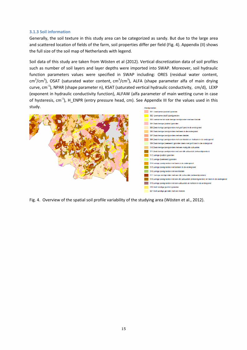
3.1.3 Soil information

Generally, the soil texture in this study area can be categorized as sandy. But due to the large area

and scattered location of fields of the farm, soil properties differ per field (Fig. 4). Appendix (II) shows

the full size of the soil map of Netherlands with legend.

Soil data of this study are taken from Wösten et al (2012). Vertical discretization data of soil profiles

such as number of soil layers and layer depths were imported into SWAP. Moreover, soil hydraulic

function parameters values were specified in SWAP including: ORES (residual water content,

cm3/cm3), OSAT (saturated water content, cm3/cm3), ALFA (shape parameter alfa of main drying

curve, cm-1), NPAR (shape parameter n), KSAT (saturated vertical hydraulic conductivity, cm/d), LEXP

(exponent in hydraulic conductivity function), ALFAW (alfa parameter of main wetting curve in case

of hysteresis, cm-1), H_ENPR (entry pressure head, cm). See Appendix III for the values used in this

study.

Fig. 4. Overview of the spatial soil profile variability of the studying area (Wösten et al., 2012).

16

3.2 Structure of WOFOST

The model WOFOST (WOrld FOod STudies) was used for crop simulation in this study. Most part of

this section was from the WOFOST model manual (Boogaard et al., 2014). WOFOST is a carbon-driven

crop growth simulation model with a time step of one day. WOFOST simulates the growth of an

annual crop with a series of specific soil and weather data. The mechanism of the WOFOST

simulation is generated from main eco-physiological processes including: phenological development,

light interception, carbon dioxide assimilation, evapotranspiration, respiration, distribution of

assimilates to organs, and dry matter formation (Fig. 5). In WOFOST potential production and limited

production (nutrient & water) can be simulated. Weeds and pests are not taken into account

(Boogaard et al., 2014).

Fig. 5. Simplified structure of WOFOST (Boogaard et al., 2014).

17

3.2.1 Phenological development

In WOFOST, phenological development is described by the order and the rate of vegetative and reproductive organs appearances. The order is independent of crop characteristics and the rate depends on crop characteristics in addition to temperature and photoperiod. In WOFOST development stage (DVS) is the descriptive variable for phenology. DVS is fixed at 0 for emergence, 1 at anthesis and 2 at maturity. WOFOST uses temperature sum to illustrate the effect of temperature on development rate. Several thermal time concepts applied here included: Te (daily effective temperature after emergence) ; T (daily average temperature); Tbase (base temperature). Besides, Te

remains constant when the temperature is above a certain maximum effective value (Tmax-e), Between Tmax,e and Tbase, the daily thermal time increase is calculated by linear interpolation (Fig. 6). The development rate (DVR) is obtained by the formula = 𝑇𝑒/𝑇𝑟𝑒𝑞, where Treq is the thermal time required to enter the next development stage. The DVR of potato is also influenced by photoperiod (P) as calculated by the eq 2:

𝐹𝑝𝑟=(𝑃−𝑃𝑐)/(𝑃𝑜−𝑃𝑐); 0≤ 𝐹𝑝𝑟≤1

𝐷𝑉𝑅=𝐹𝑝𝑟 (𝑇𝑒/𝑇𝑟𝑒𝑞) Eq 2

‘where Fpr is the photoperiod reduction factor for the development rate until flowering, Po is optimum photoperiod and Pc is critical photoperiod’(Boogaard et al., 2014).

Fig. 6. Relation between daily average temperature (°C) and daily increase in the thermal time [°C*d],

for the calculation of the development stage of a potato crop (Tbase = 2 °C, Tmax,e = 28 °C) (modified

from Boogaard et al., 2014).

3.2.2 Light interception and assimilation

WOFOST uses absorbed radiation (Ia) and the photosynthesis-light response curve of individual

leaves to calculate daily CO2-assimilation rate. Temperature and leaf age determine the response

curve. Total incoming radiation and the leaf area determine the absorbed radiation. There are two

factors influencing photosynthesis response to light intensity. The first factor relates to the different

levels of lights received in the canopy along the vertical plane. To calculate this, the canopy is divided

0

5

10

15

20

25

30

0 5 10 15 20 25 30 35 40

dai

ly in

crea

se in

th

erm

al t

ime

(℃*d

)

daily average temperature (℃*d)

Tb Tmax,e

18

into different layers. At each leaf layer, intercepted light is derived from the radiation flux at the top

of the canopy and the transmission by overlying layers. The other factor is temporal, caused by the

daily cycle of sun. WOFOST uses the eq 3 to simulate the mentioned two factors:

𝐼0=𝐼 sin𝛽

𝐼𝑎𝐿=𝑑𝐼𝐿/𝑑𝐿=(1−𝜌)𝐼0𝑒−𝑘𝐿𝐴𝐼𝐿 Eq 3

‘where I0 is the radiation level at the top of the canopy on a clear day; 𝛽 is sine of the angle between

the sun and the earth’s surface; IaL is the adsorbed radiation by leaf layer L; IL is the net radiation flux

at depth L; k is the extinction coefficient; ρ is a reflection coefficient which is a function of solar

elevation, leaf angle distribution, and reflection and transmission properties of the leaves; LAIL is the

cumulative leaf area index at depth L ([m2 (leaf) m-2 (ground)]. (Boogaard et al., 2014).’ After the light

interception is settled, the instantaneous assimilation rate of a leaf layer can be calculated by the eq

4:

𝐴𝐿=(1−𝑒−𝜀(𝐼𝑎𝐿/𝐴𝑚)) Eq 4

‘Where AL is the gross assimilation rate [kg (CO2) m-2 (leaf) s-1]; Am is the maximum gross assimilation

rate; ε is the initial light use efficiency [kg (CO2) J-1’(Spitters et al., 1989);

By integrating the assimilation rates over layers and time, daily gross CO2 assimilation is obtained. In

this procedure, it is assumed that incoming radiation over the day is a sinusoidal course and a three-

point Gaussian integration method (Goudriaan, 1986) is performed. Part of the assimilates are used

for maintenance respiration, which is estimated based on the dry weight of different organs and

their chemical composition. Assimilates are distributed to different organs and the assimilate

partitioning is determined by the development stage (Fig. 7) (Penning de Vries, 1975; Penning de

Vries et al., 1989).

Fig. 7. An example of assimilates distribution by different development stages (Boogaard et al., 2014).

19

3.3 Structure of SWAP

The model SWAP (Soil Water Atmosphere Plant) was used for the hydrological simulation in this

study. Most part of this section was from the SWAP manual (Van Dam et al., 2008). SWAP is an agro-

hydrological model (Fig. 8). SWAP simulates transport of water, heat and solute in the vadose zone in

interaction with vegetation development (Van Dam et al., 2008). SWAP is designed to simulate the

transport process at field level during the growing season and it is a one-dimensional, vertically

directed model. SWAP can be applied to plan irrigation, including timing criteria and depth criteria.

SWAP requires inputs such as meteorological data, crop growth and drainage (Van Dam et al., 2008).

Fig. 8. SWAP model domain and transport process (Van Dam et al., 2008)

3.3.1 Soil water flow and bottom boundary condition

SWAP uses Darcy’s eq to quantify vertical soil water fluxes (eq 5):

𝑞 = −𝐾(ℎ)𝜕(ℎ+𝑧)

𝜕𝑧 Eq 5

‘where q is soil water flux density (positive upward) (cm d-1), K(h) is hydraulic conductivity (cm d-1), h is

soil water pressure head (cm) and z is the vertical coordinate (cm), taken positively upward (Van Dam

et al., 2008)’.

By considering soil volume as infinitely small, the continuity eq for soil water is obtained (eq 6):

𝜕𝜃

𝜕𝑡= −

𝜕𝑞

𝜕𝑧− 𝑆𝑎(ℎ) − 𝑆𝑑(ℎ) − 𝑆𝑚(ℎ) Eq 6

‘where θ is volumetric water content (cm3 cm-3), t is time (d), Sa(h) is soil water extraction rate by

plant roots (cm3 cm-3 d-1), Sd (h) is the extraction rate by drain discharge in the saturated zone (d-1)

and Sm(h) is the exchange rate with macro pores (d-1)’ (Van Dam et al., 2008).

20

By combing the eq (5) and eq (6), general soil water flow was generated as Richard’s eq (7):

𝜕𝜃

𝜕𝑡= −

𝜕[𝐾(ℎ)(𝜕ℎ

𝜕𝑧+1)]

𝜕𝑧− 𝑆𝑎(ℎ) − 𝑆𝑑(ℎ) − 𝑆𝑚(ℎ) Eq 7

SWAP solves Richards’s eq numerically with the known relation between θ, h and K. Richard’s eq is

applied in SWAP integrally for the unsaturated-saturated zone. More detail information can be found

in the SWAP manual.

As for bottom boundary conditions, one of the options is to prescribe groundwater levels. A field-

averaged ground water level (φavg) is given as a function of time. SWAP linearly interpolates between

the dates and times at which the groundwater levels are specified.

3.3.2 Rainfall interception and evapotranspiration

SWAP simulates intercepted precipitation by the eq proposed by Von Hoyningen-Hüne (1983) and

Braden (1985) (eq 8):

𝑃𝑖 = 𝑎 ∙ 𝐿𝐴𝐼(1 −1

1+𝑏∙𝑃𝑔𝑟𝑜𝑠𝑠

𝑎∙𝐿𝐴𝐼

) Eq 8

‘where Pi is intercepted precipitation (cm d-1), LAI is leaf area index, Pgross is gross precipitation (cm d-1),

a is an empirical coefficient (cm d-1) and b is the soil cover fraction (-)’ (Van Dam et al., 2008).

According to eq 8 intercepted precipitation can asymptotically reach to the saturation amount (a∙LAI)

by increasing precipitation amounts. In principle, coefficient a must be determined by experiment

and specified in the input file. For the ordinary agriculture crops, a is assumed as 0.025 cm d-1.

Coefficient b is estimated by eq 9:

𝑏 = 1 − 𝑒−𝐾𝑔𝑟𝐿𝐴𝐼 Eq 9

‘where b is the soil cover fraction and Kgr is the extinction coefficient for solar radiation’(Van Dam et

al., 2008)

As for evapotranspiration, it refers to transpiration of plants and evaporation from the soil or

ponding on the soil surface. It is assumed that root water extraction is equal to plant transpiration,

because the water fluxes trough the canopy are larger than what is stored. The Penman-Monteith eq

has become an international standard of potential evapotranspiration, due to its best performance in

all kinds of climate conditions. Therefore, in SWAP the Penman-Monteith eq is used to calculate

evapotranspiration (eq. 10):

𝐸𝑇𝑃 =

∆𝑣𝜆𝑤

(𝑅𝑛−𝐺)+𝑝1𝜌𝑎𝑖𝑟𝐶𝑎𝑖𝑟

𝜆𝑤

𝑒𝑠𝑎𝑡−𝑒𝑎𝑟𝑎𝑖𝑟

Δ𝑣+Υ(1+𝑟𝑐𝑟𝑜𝑝

𝑟𝑎𝑖𝑟)

Eq 10

‘where ETp is the potential transpiration rate of the canopy (mm d-1), Δv is the slope of the vapour

pressure curve (kPa °C-1), λw is the latent heat of vaporization (J kg-1), Rn is the net radiation flux at the

canopy surface (J m-2 d-1), G is the soil heat flux (J m-2 d-1), p1 accounts for unit conversion (=86400 s d-

1), ρair is the air density (kg m-3), Cair is the heat capacity of moist air (J kg-1 °C-1), esat is the saturation

vapour pressure (kPa), ea is the actual vapour pressure (kPa), γair is the psychrometric constant

(kPa °C-1), rcrop is the crop resistance (s m-1) and rair is the aerodynamic resistance (s m-1)’ (Van Dam et

al., 2008).

21

The estimation of potential and actual evapotranspiration is possible with the Penman-Monteith eq,

but this approach requires canopy and air resistance which is not available for many crops. Therefore,

SWAP uses two steps to calculate actual evapotranspiration. The first step is the calculation of

potential evapotranspiration with the minimum value of canopy resistance and the actual air

resistance. Detailed information on this step can be found in the SWAP manual. The second step is to

calculate actual evapotranspiration by taking into account of root water uptake due to water and/or

salinity stress. The potential root water uptake is calculated in SWAP as follows:

𝑆𝑝(𝑧) =𝜄𝑟𝑜𝑜𝑡(𝑧)

∫ 𝜄𝑟𝑜𝑜𝑡(𝑧)𝑑𝑧0−𝐷𝑟𝑜𝑜𝑡

𝑇𝑝 Eq 11

‘where Sp(z) is the potential root water extraction rate at a certain depth, lroot(z) is ,Droot is the root

layer thickness, Tp is potential evapotranspiration’(Van Dam et al., 2008).

Sp(z) can be reduced by stress of dry or wet conditions, which is explained in the next section.

3.3.3 Water stress and oxygen stress

In SWAP, water stress is described by the function proposed by Feddes et al. (1978), which is

interpreted in Fig. 9. In the range of h3<h<h2, water uptake is optimal. Below h3 water uptake linearly

decreases due to drought stress until point h4 (wilting point). Above h2 water uptake linearly

decreases due to insufficient aeration until 0 at h1. The critical pressure head h3 increases for higher

potential transpiration Tp (Fig. 9).

Fig. 9. Reduction coefficient for root water uptake, αrw, as function of soil water pressure head h and

potential transpiration rate Tp (Feddes et al., 1978).

In this study, salinity is not taken into account, so the actual root water flux Sa(z) (d-1) is calculated as:

𝑆𝑎(𝑧) = 𝛼𝑟𝑤𝑆𝑝 Eq 12

‘where arw is dimensionless water stress coefficient’ (Van Dam et al., 2008)

Besides, in SWAP the maximum evaporation rate that the top soil can sustain is calculated by Darcy’s

law:

𝐸max = 𝐾1

2

(ℎ𝑎𝑡𝑚−ℎ1−𝑍1

𝑧1) Eq 13

22

‘where K½ is the average hydraulic conductivity (cm d-1) between the soil surface and the first node,

hatm is the soil water pressure head (cm) in equilibrium with the air relative humidity, h1 is the soil

water pressure head (cm) of the first node, and z1 is the soil depth (cm) at the first node’(Van Dam et

al., 2008).

The function of Feddes et al. (1978) is also generally used for oxygen stress assessment. But the

Feddes-function does not combine plant physiological and soil physical processes to predict the

reduction of root water uptake at insufficient soil aeration (Bartholomeus et al., 2008). Thus,

Bartholomeus et al. (2008) proposed a plant physiological and soil physical process-based model to

determine the minimum gas filled porosity of the soil (ɸgas_min) when oxygen stress occurs. In this

model, they calculated the minimum oxygen concentration in the soil to just sustain roots respiration

(micro-scale) and calculated ɸgas_min diffusion from the atmosphere through the soil (macro-scale)

which relates to the minimum oxygen concentration (Fig. 10). Also, in the model they included soil

type, temperature, organic matter content, soil depth and plant characteristics. They compared the

result with the Feddes-function and drew a conclusion that this model based method is better

because the Feddes-function might lead to large errors in the prediction of transpiration reduction

and growth reduction through oxygen stress. Furthermore, they implemented the model into SWAP

to improve the simulation root water uptake and root growth.

Fig. 10. Scheme for the calculation of critical values for oxygen stress, based on both physiological

and physical processes (Bartholomeus et al., 2008).

23

3.4 WOFOST Calibration for Potential Yield

Before using SWAP-WOFOST to investigate the impact of water and oxygen limitation on potato

yields, the crop growth model WOFOST needs to be calibrated. This is because default model

parameters are based on experiments from more than 20 years ago (Boons-Prins et al. 1993,

Boogaard et al. 2014), and currently observed yields are higher than the simulated potential.

3.4.1 Fields and Data

For WOFOST calibration, the cultivar Fontane was selected because it was widely planted in the years

2013 and 2014, and yields were higher compared to other cultivars. The data of the year 2014 were

used for calibration while data from the year 2013 was used for validation. Nine fields were selected

with a yield range of 87-105 t/ha. Because of data noise, among these 9 fields, 3 fields were selected:

“geudens windmolens”, “wauters achter stal” and “fabrie arendonk”. Tuber yield was measured five

times during the growing season (Fig. 11). The sowing date and date of harvest the nine different

fields varied, with a range of 22 and 29 days respectively. The measurement dates were similar (one

to three days difference) for the same measurement in different fields. However, the records of the

second and third measurement dates were incomplete. It was assumed that the missing date is

around the date of nearby fields based on other records at the farm level. Moreover, the fourth

measurement date differed up to 30 days (Fig. 12).

Fig. 11. Observed WSO (dry matter weight of storage organs) of different fields by different

measurement times (some measurement days are unavailable) for calibration.

Fig. 12. Different planting and yield measurement days of the nine fields (some measurement days

are unavailable).

0

5000

10000

15000

20000

25000

0 1 2 3 4 5 6

WSO

kg/

ha

Mark hurkmans

wauters achter stal

fons tegen hans dirks

fabrie arendonk

obroek

geudens windmolens

vermeulen hulsel

jef adrjaanse werbeek

jef dirks achterstal 1

0

50

100

150

200

250

300

Day

Fields

Planting date

Measurement Day 1

Measurement Day 2

Measurement Day 3

Measurement Day 4

24

No experiment was done for potential production circumstances, so it was assumed that highest

yields were close to the potential. In order to make a representative and reliable model calibration,

several fields were selected. The criterion of fields selection for potential yield calibration was based

on the achieved highest yield. As for the data for calibration, fresh tuber yield was measured five

times for all the fields during the whole growing period in year 2014. Also under water tuber weight

(UWW) of most fields were available which can be used for dry matter content calculation. In this

study dry matter content of tuber was calculated as UWW/18 (De Wilde et al., 2006). Data of tuber

yield was the key input for calibration. Additionally, phenology such as emergence and maturity were

observed for some fields which can be used for phenological calibration. Pictures were made during

the growing season in several fields, which allowed to determine emergence and flowing. However,

these fields were not the same as the 9 fields selected.

3.4.2 Potential yield without calibration

As a starting point, potential yield was simulated in WOFOST control center (version 2.1.2) with the

crop file “Potato 701”. The simulation periods correspond to the fields selected for calibration. After

simulating the potential yield with default model parameters in 2014, model performance was

evaluated by model efficiency.

3.4.3 Model Parameters

Parameters were selected according to the WOFOST calibration manual (Wolf, 2003) as follows:

TSUMEM (temperature sum from sowing to emergence), TSUM1 (the temperature sum from

emergence to anthesis), TSUM2 (the temperature sum from anthesis to maturity), AMAXTB

(maximum leaf CO2 assimilation rate as a function of development stage of the crop), SPAN (life span

of leaves), SLATB (specific leaf area) and assimilates partitioning factors: FSTB (fraction stems), FOTB

(fraction organs) and FLTB (fraction leaves). LAI (leaf area index), was not selected due to the limited

data availability.

Wolf (2003) gave the procedure for WOFOST calibration. The model calibration should be done in

orders due to the variation of the model variables. Ideally, the model calibration needs to be done

first for a potential production situation and second for the water limited production. However, in

this study specifically water limited production experiments had not been designed and performed,

therefore the calibration was done only for potential yield production.

3.4.4 Parameter sensitivity

Before the calibration, a sensitivity analysis was performed to rank the parameters in order of

importance for TWSO (total dry weight of storage organs). In this sensitivity analysis only one

parameter was changed each time with 5% (Increase & decrease) of the initial value with a total 9

reruns.

3.4.5 Calibration procedure

The calibration is in the following order:

I. Length of growing period and phenology. In this procedure, the sowing date or crop emergence is

essential phenology input for WOFOST. In this study, TSUMEM was calibrated first. Based on the

farm records, the sowing and emergence dates of several fields (the link to the source data were

deleted by farmer so the number of the fields is unknown) were available for TSUMEM calibration.

Emergence was observed at day 126 & 133 for sowing day 99 and 141 for sowing day 118. The

25

sowing dates 99 and 118, were used as input in WOFOST. Other parameters that were calibrated in

this procedure were TSUM1, SPAN and TSUM2. Fields for TSUM1 calibration were the same as for

the TSUMEM calibration. However, there were no records of anthesis for these fields. Indirectly, a

picture of anthesis (around day 171) was found for the fields with planting day of 118. In WOFOST, in

order to ignore the influence from planting to emergence, a fixed emergence day of 141 (observed

emergence day) was used. In order to keep coherence, the SPAN value was calibrated considering

the results of previous steps (TSUMEM=220 ℃, TSUM1= 420 ℃), and with a fixed planting day of 118.

As for TSUM2 calibration, the default value TSUM2 1550 ℃ was tested first, with the parameter’s

results of previous steps. In order to make the TSUM2 calibration representative and precise, all the

fields in the farm available with observed maturity were chosen, averaged and classified into 7

groups. Each group represents the same sowing day. The difference of sowing dates between the

consecutive groups was about 5-10 days. The number of the fields in each group depends on the

data and was not exactly the same. In the farm, crop stages were recorded as values between 0-10,

in this study, crop stage 10 indicates crop maturity.

II. Light interception and potential biomass production. In this procedure, LAI (leaf area index) should

be calibrated to reproduce the observed value and the related parameter is SLATB (specific leaf area)

which converts leaf mass in leaf area using the rerun facility in WOFOST. After that the total crop

biomass will be calibrated (TAGP) using parameter AMAXTB (maximum leaf CO2 assimilation rate as

a function of development stage of the crop).

In the step of AMAXTB calibration, the calibrated parameters values of previous steps were imported

(phenology parameters). However, the planting, ending (haulm killing) and tuber yield measurement

dates were different for the 9 fields. In order to simplify the AMAXTB calibration procedure, 3

(“geudens windmolens”, “wauters achter stal” and “fabrie arendonk”) among the 9 fields were

selected based on the criteria of a linear tuber yield growth trend and similar growing period,

because it is assumed that accumulative potential yield is linear increased with time course. Also the

data of the three fields were averaged including sowing, ending and measurement dates and the

measured WSO (dry weight of storage organs) values. AMAXTB calibration was first done for the 3

fields, and then evaluated for all the 9 fields until model performance was well enough for most of

the fields.

III. Assimilate distribution between crop organs. In this part, the Harvest Index (HI) needs to be

calibrated. The model parameters related to the partitioning are the FSTB (fraction stems), FOTB

(fraction organs) and FLTB (fraction leaves), which are a function of the development stage (DVS).

3.5 Potential yield validation

To validate the calibration, data of the same cultivar Fontane from 2013 were used. Similar to the

calibration, 5 fields with highest yields were chosen for validation. In 2013, fresh tuber yield and

under water tuber weight were measured 4 times during the growing season, these values were

transformed to dry matter yield with the same function, which is the only indicator for validation.

The fresh tuber yields ranged from 80.35 to 95.21 t/ha (Fig. 13). Planting dates, ending dates and

WSO measurements dates were similar for these fields, but some dates data were unavailable. WSO

was measured for four times (Fig. 14).

26

Fig. 13. Observed highest yields (FM t/ha) in year 2013.

Fig. 14. Observed WSO (DM t/ha) of the five fields with highest yield in 2013.

3.6 Additional statistic methods

Evaluation of model performance was first done by visual assessment. Statistic methods were also

used to evaluate parameter values and model efficiency through calibration, including SSE (sum of

squared errors; eq 14) and EF (model efficiency; eq 15). Model performance is considered excellent if

EF is higher than 0.9, acceptable if 0.8<EF<0.9, poor if EF<0.8

𝑆𝑆𝐸 = ∑ [𝑌𝑖,𝑜𝑏𝑠 (𝑋𝑖) − 𝑌𝑖.𝑝𝑟𝑒𝑑 (𝑋𝑖 , 𝑃)]2𝑁

𝑖=1 Eq 14

𝐸𝐹 =∑ (𝑂𝑏𝑠𝑖−𝑂𝑏𝑠)

2−∑ (𝑃𝑟𝑒𝑑𝑖−𝑂𝑏𝑠)

2𝑛𝑖=1

𝑛𝑖=1

∑ (𝑂𝑏𝑠𝑖−𝑂𝑏𝑠)2𝑛

𝑖=1

Eq 15

where obs is observation, obsis the mean of obs, pred is prediction (Reidsma et al., 2012).

0

20

40

60

80

100

houbraken spietegen bos

geudens aan huis tim kijzers hoef tim nieuwen dijk fabrie gemeentehoef

FM Y

ield

(t/

ha)

Fields

0

5

10

15

20

0 1 2 3 4 5

WSO

(t/

ha)

Measurement time

houbraken spie tegen bos geudens aan huis tim kijzers hoeftim nieuwen dijk fabrie gemeente hoef

27

3.7 Drought & oxygen stress simulation

After WOFOST calibration and validation, drought & oxygen stress simulation were performed.

As for water stress fields selection, unfortunately, no drought or oxygen stress trials were designed

and performed in the farm. It was unclear which fields were certainly under water stress. Therefore a

series of approaches were applied to select the fields which were possibly under water stress. Fields

were selected using the following criteria: I: Actual yields and average yield were compared first;

fields with yield under average were desirable choices. II: Secondly, the initial drought sensitivity

assessment was taken into account; fields graded as dry and wet were ideal choices. III: Nutrient

condition was another factor considered; initial field nutrients were assessed in the farm as poor,

average and rich; fields marked as average and rich were better options. VI: In order to make the

fields more representative and diverse, the location and the soil types of fields were also considered.

Fields with different locations and different vertical soil profiles were more desirable options. V:

Constrained by the data availability, fields closer to a metrological station (Dacom) and ground water

level monitoring station were chosen. Moreover, the farmer’s opinion was also taken into

consideration. However, as the ground water level data and soil data were unavailable for Belgium,

fields in Belgium were not taken into account. Simulations were performed both for the year 2013 &

2014. As a result, 10 fields were selected in 2013 and 17 fields in 2014.

Data used for the simulations were as follows: I: Initial drought sensitivity of different fields were

assessed by the farmer as average, drought, and wet. Weather data were accessed from

meteorological station Eindhoven. Parts of the precipitation data from Dacom were supplementary

input for different fields. Most of the fields were within a distance of 10 km from a Dacom station

(Appendix IV). Precipitation data recorded at fields "Blokseschuur tegen bos" and "Cor weg eersel"

were used for simulations in 2013. As for 2014, precipitation data measured from Eindhoven and at

fields “Voorsteheide”, “Johan kuipers voorhuis” and “Jan luiksgestel achter bos” were used. Detailed

information of the actual rainfall data used can be found in Appendix I. Soil property data were

explained in section 3.1.3. In total, 15 different sol profiles were used in the simulations. Detailed soil

data can be found in Appendix IV & V. Ground water level data were obtained from the Dino Loket

website (https://www.dinoloket.nl/) and they were used to define the bottom boundary condition

and the initial water content indirectly as a function in SWAP.

The models WOFOST and SWAP were integrated into SWAP-WOFOST for the simulations. Farm

management was also specified for each field including sowing date, ending date and irrigation

information (date & amount).

For the drought stress, simulations were first done without irrigation. Then in another round,

simulations were done with irrigation. A comparison was done between the two types of simulations

to find out the yield gap closure by irrigation. As for oxygen stress simulations, the procedure was

similar as the drought stress simulations; non-drainage simulations were done first and followed with

simulations with drainage, depending on the simulation results. Comparisons were also done for the

different simulation scenarios.

28

Fig. 15. Observed yield of the selected fields for water stress simulation in 2013

Fig. 16. Observed yield of the selected fields for water stress simulation in 2014

3.7.1 Drought stress sensitivity to precipitation and soil

In order to test the drought stress sensitivity to soil profile, simulations were done with the following

settings: using weather data of 2013 and 2014 from Eindhoven to simulate the water limited yield for

all the different soil types in this study. Within the same year, the influence of different soil inputs on

yield can be compared. Between different years, the influence of different weather can be compared.

But the impact of precipitation still cannot be presented. Thus another scenario was applied: in the

year 2013, the water limited of field (“fabri lutter gemeente”) with different precipitation data from

Dacom (“blokseschuur tegen bos” & “cor weg eersel”) were simulated and compared. Therefore, the

impact of precipitation and soil inputs were both investigated.

3.7.2 Pressure head and ground water level

As described in section 3.3.3, SWAP-WOFOST uses soil water pressure head values to indicate

drought and oxygen stress. However, it is unclear whether the model default values of pressure head

(h) can be used directly without amendment. Therefore, sensitivity analyses were performed to

evaluate the relationship between h and water limited yield. Value of h was increased or decreased

0102030405060708090

Yiel

d (

t/h

a)

Field name

Average yield

0

20

40

60

80

100

120

Yiel

d (

t/h

a)

Field name

Average yield

29

with 1% or 10 % each time. Sensitivity analyses were not done for all of the different soil profiles, due

to its large amounts. Sensitivity analysis was done for field “fabri lutter gemeente” “fabrie gemeente

hoef” in 2013 and “wauters achter stal”, “v.d. sande naast schuur” in 2014.

The sensitivity of groundwater levels on water limited yield was also investigated. Two fields were

chosen for each year, one with low yield and the other one with high yield. In 2013, fields “fabri

lutter gemeente” (48.78 t/ha) and “fabrie gemeente hoef” (80.36 t/ha) were chosen. In 2014, “v.d.

sande naast schuur” (51.81 t/ha) and “wauters achter stal“(98.1 t/ha) were chosen. Ground water

levels were decreased or increased with steps of 10cm through the year.

3.7.3 Irrigation scheduling

Water balance simulation results can be used for irrigation schedules. The strategy employed in this

study is the critical pressure head or moisture content. The automated irrigation is applied when the

defined threshold is exceeded: θsensor ≤ θmin orhsensor ≤ hmin

where θsensor and hsensor are the threshold values for soil moisture and pressure head respectively (Van

Dam et al., 2008).

As for the irrigation amount, It is a function of development stage. The soil water content will back to

field capacity after automatic irrigation.

30

31

4 Results

4.1 Estimating potential yields without calibration

The potential yields of different fields were simulated using default model parameter values and

compared with the observed yields (Fig. 18). Model performance is poor and the difference between

simulation and observation varied from 16.4 % to 45.6 %, which is 15.35 t/ha and 45.8 t/ha

respectively. As yields obtained in the fields cannot be higher than the simulated potential yields,

calibration is needed to improve the simulations. Moreover, simulated potential yield of different

fields also varied due to the different growing period (sowing & ending dates).

Fig. 18. Simulated potential yields compared to observed fresh yields in the highest yielding fields in

2014 (fields were placed in order of sowing dates; dry matter content was derived from last UWW

measurement of each measurement and used to transform simulations from DM to FM).

4.2 Sensitivity analysis

The sensitivity analysis of TWSO to different parameter values was done. Only one parameter was

changed each time with 5% (increase & decrease) based on the initial value (Fig. 19). TWSO was

found most sensitive to the values of parameters TSUM2 and AMAXTB, around ±3.8 % and ±2.5 %

change in TWSO respectively with a 5% change in parameter value. Moreover, TWSO gradually

decreased while reducing SPAN value. Also, FOTB 2nd affects TWSO with approximately ±2% for each

simulation. TWSO was not found sensitive to other parameters values. As for parameter SLATB, there

are three different sub values in different DVS, thus SLATB results were presented as SLATB

combined with different DVS. Results show that influence of changing values of SLATB on TWSO is

small for all the DVS. Similarly, the parameter FOTB, FLTB, and FSTB have five different values in

different DVS. These three parameters were presented with the value changed, for instance changing

the first parameter value of FLTB was described as FLTB 1st. As for the results, the influence of FLTB

1st & 2nd , FSTB 1st ,2nd and 3rd on TWSO is small. Based on the results of sensitivity analysis, following

step of WOFOST model calibration will focus more on the parameters AMAXTB, TSUM2, SPAN and

FOTB 2nd.

0

20

40

60

80

100

120

Yiel

d (

t/h

a)

Fields

Simulation Observation

32

Fig. 19. Sensitivity of TWSO compared to initial default value by changing one parameter value 5%

each time.

4.3 WOFOST calibration for potential yield simulation

4.3.1 TSUMEM calibration

Five different TSUMEM values (170 ℃ (default), 200 ℃, 220 ℃, 240 ℃, 260 ℃) were tested and

compared (Fig. 20). TSUMEM 240 ℃ has the lowest SSE of 13, whereas SSE of TSUMEM 260 ℃ was

16, for TSUMEM of 220 ℃ it was 17, for TSUMEM of 200 ℃ it was 49 and for TSUMEM 170 ℃ it was

104. TSUMEM 220 ℃ was chosen even though its SSE was not the lowest, because the first observed

emergence day varied (126 & 133) which influenced the results of SSE which are based on the

average of both. If the first emergence day of 126 would be taken, TSUMEM 220 ℃ is the best value

matching the reality.

Fig. 20. Observed (OB) and simulated (SM) emergence day with two different planting days.

-20

-15

-10

-5

0

5

10

15

-20 -15 -10 -5 0 5 10 15 20

Value of parameter changed (%)

TWSO changed (%)

AMAXTB SLATB DVS=0 SLATB DVS=1.1 SLATB DVS=2 TSUM1

TSUM2 FLTB 1st FLTB 2nd FSTB 1st FSTB 2nd

FSTB 3rd SPAN FOTB 2nd

120

125

130

135

140

145

150

120 125 130 135 140 145

SM e

mer

gen

ce d

ay

OB emergence day

OB Emergence Day

SM TSUMEM 170

SM TSUMEM 200

SM TSUMEM 220

SM TSUMEM 240

SM TSUMEM 260

33

4.3.2 TSUM1 calibration

Five different TSUM1 values were tested (150 ℃, 300 ℃, 350 ℃, 420 ℃, 440 ℃) and compared with

the observed anthesis day (Fig. 21). With default TSUM 1 (150 ℃), simulated anthesis differed 18

days with observation (Fig. 21). TSUM1 of 420 ℃ was selected and it was “spot on”.

Fig. 21. Observed and simulated anthesis day with different TSUM1 values.

4.3.4 TSUM2 calibration

With the default TSUM2, simulated maturity days varied (3-9 days) from the observations which led

to the following calibration. Seven different TSUM2 values were tested and compared with the

observed maturity day (Fig. 22). The SSE of TUSM2 1450℃ was lowest and SSE of TSUM2 1600 ℃ was

largest (Appendix VI). Besides, the results of group 3 and group 7 were very different from others,

the possible reason could be the different sowing depths or the initial tuber size.

Fig. 22. Observed and simulated maturity with different TSUM2 values.

4.3.3 SPAN calibration

With a default SPAN value of 37 days, the results shows that LAI decreased sharply at day 262.

However, according to the observation, with a sowing day of 118, leaves remained green and haulm

killing was used to eliminate leaves at day 270. So SPAN needed to be enlarged to match reality. In

this section, four different SPAN values were tested and compared with the observed maturity day.

The decreasing point of LAI at the end of the growing season is the reference maturity day according

150 155 160 165 170 175

Anthesis day

OB anthesis

SM TSUM1=150 ℃

SM TSUM1=300 ℃

SM TSUM1=350 ℃

SM TSUM1=420 ℃

SM TSUM1=440 ℃

245

250

255

260

265

270

275

280

245 250 255 260 265

SM M

atu

rity

Day

OB Maturity Day

1:1 line

TSUM2=1400 ℃

TSUM2=1420 ℃

TSUM2=1450 ℃

TSUM2=1470 ℃

TSUM2=1500 ℃

TSUM2=1550 ℃

TSUM2=1600 ℃

34

to WOFOST. Observed average maturity was at day 270 for the sowing day 118 across the farm. In

the simulation, the growing periods (sowing to maturity) of all the SPAN values under 41 days were

shorter than the observation (Fig. 23). Thus, SPAN should be taken larger than 41. As there were

variances in the fields, some had a late maturity than day 270. Hence, a SPAN value of 43 was chosen.

Fig. 23. Life span of leaves with different SPAN values (default SPAN=37 blue; SPAN=39 orange;

SPAN=41 red; SPAN=43 green)

4.3.5 AMAXTB calibration

Parameter values were taken based on the previous calibration results (TSUMEM=220 ℃,

TSUM1=420 ℃, TSUM2=1450 ℃, SPAN 43 days), and several different combined AMAXTB values

were tested and compared with the observed WSO (Fig. 25). Model efficiency (0.9819, 0.9810,

0.9847) was only evaluated for simulations 5, 6 and 7 while simulations 1-4 were assessed visually

due to its poor performance. Parameter AMAXTB values are a function of DVS of the crop. There are

three different DVS (0.00; 1.57; 2.00) related to AMAXTB of potato in WOFOST. The overview of the

parameter values changed during the AMAXTB calibration was summarized (Table. 1).

SM1 SM2 SM3 SM4 SM5 SM6 SM7

AMAXTB 30; 30; 0 65; 65; 65 65; 65; 20 200;200;20 65; 65; 0 65; 65; 0 47; 47; 0

TSUM1 420 ℃ 420 ℃ 420 ℃ 420 ℃ 320 ℃ 320 ℃ 320 ℃

TSUM2 1450 ℃ 1450 ℃ 1450 ℃ 1450 ℃ 1450 ℃ 1650 ℃ 1650 ℃

Table 1. Values of parameter changed (indicated in red) during AMAXTB calibration.

35

AMAXTB with default values (30; 30; 0) was tested first (SM1) and results show that simulated TWSO

was much lower (5686 Kg/ha, DM) than the observation (fig. 25). AMAXTB should be increased to

reach a higher production level. AMAXTB (65; 65; 65) was tested secondly (SM2), but the results of

the last two simulation points were too high (757 and 2235 Kg/ha, DM). In order to decrease the

simulated WSO in later stage of the growing period, the third value of AMAXTB was decreased:

AMAXTB (65; 65; 20) was tested (SM3). The results show that the last two simulations points

decreased, but the first two were too low (1397 and 1680 Kg/ha, DM). In other words, the first two

AMAXTB values need to be increased to achieve higher WSO in early tuber growth stage. Increasing

AMAXTB (200; 200; 20), the first two simulated (SM4) values were still much lower (1331 and 1457

Kg/ha, DM) compared to the observation. As even with the first two values of AMAXTB to be 200

there was no significant improvement in the simulated values of the first two WSO, which means

AMAXTB was apparently not the constraint in this growing phase.

There are two constraints for WSO accumulating; phenology and AMAXTB. In terms of phenology, an

early tuber initiation will enable a longer period for tuber growth, which means a lower TSUM1 value.

Hence, TSUM1 was decreased from 420 ℃ to several different values and tested with AMAXTB (65;

65; 0). With TSUM1=320 ℃ life span was 10 days shorter than the observation (SM5), but model

efficiency reached 0.9819. In order to have a longer life span, parameter TSUM2 was increased to

several different values and tested. Within these different values, in SM6, TSUM2 was increased to

1650 ℃ and with the same AMAXTB (65; 65; 0), model efficiency was 0.9810 and life span matched

with reality, but the last two points of simulation were too high compared to the observation. Several

AMAXTB values were tested again based on the new phenology parameter settings. As a result,

ranges of the first two AMAXTB values (around 44-55) were found to reach high model efficiency

(higher than 0.98). Reducing AMAXTB to (47; 47; 0), model efficiency slightly increased to 0.9847

(SM7). Since there was no significant difference in values around 47 kg/ha.hr, AMAXTB (47; 47; 0)

was chosen after the calibration.

Model efficiency of the AMAXTB calibration was based on the data of three fields among all nine

fields with highest yields. In order to check the model performance for all of the chosen fields with

highest yield, after the AMAXTB calibration was done, all of the calibrated model parameters were

included for the potential yield simulations. Simulated potential yields were compared with all the

nine fields, specifically for the individual growing periods and tuber yield measurements (Fig. 26).

Model efficiency was evaluated for all of the nine fields (Fig. 27). The model performed well for six

fields with a model efficiency range of 0.84-0.94. However, model efficiency for the field “obroek”

was only 0.69, for the field “fons tegen hans dirks” it was 0.43 and for field “vermeulen hulsel” it was

0.29. As for the results of fields with poor model efficiency, especially for the field “vermeulen hulsel”,

the model underestimated reality to a great extent. The most possible reason is that the model

calibration was based on the criterion of linearly growing trend, whereas the observation values

were not. Also, the other fields chosen for calibration had relatively lower yields compared to this

one.

36

Fig. 25. Mean observed WSO of three selected fields and simulated WSO with different AMAXTB

values (SM1 was the default).

Fig. 26. Observed WSO of nine fields and simulated WSO with the calibrated AMAXTB.

Fig. 27. Model efficiency for different fields with calibrated model parameters in 2014.

0

5000

10000

15000

20000

25000

0 5000 10000 15000 20000

Sim

ula

tio

n (

kg/h

a)

Observation (kg/ha)

1:1 line

SM 1

SM 2

Sm 3

SM 4

SM 5

SM 6

SM 7

0

5000

10000

15000

20000

25000

0 5000 10000 15000 20000 25000

Sim

ula

tio

n (

kg/h

a)

Observation (kg/ha)

1:1 line

vermeulen hulsel

Mark hurkmans

wauters achter stal

fons tegen hans dirks

fabrie arendonk

geudens windmolens

jef dirks achterstal 1

jef adrjaanse werbeek

obroek

0

0.5

1vermeulen hulsel

Mark hurkmans

wauters achter stal

fons tegen hans dirks

fabrie arendonkobroek

geudens windmolens

jef dirks achterstal 1

jef adrjaanse werbeek

37

4.3.6 WOFOST validation

The calibrated model was validated with the data of selected five fields with highest yield in 2013 (Fig.

28). Due to the different growing periods and measurement dates, validation was performed for

each field specifically. Model efficiency was considered excellent for most of the fields (4 out of 5).

Field “fabrie gemeente hoef” and “houbraken spie tegen bos” reached a model efficiency of 0.95 and

0.93 respectively, model efficiency of fields “geudens aan huis” and “tim kijzers hoef” were both 0.89

and acceptable. However, model efficiency of field “tim nieuwen dijk” was poor, only 0.76. In general,

model validation results show that calibration was well enough for the year 2013. However, one

good validation for one year is no guarantee that the model is successfully calibrated for the long

term period. The weather in both years was quite different however, especially the start of the spring.

Highest yields in 2014 were 7 to 10 t/ha higher than in 2013, and this difference was well reflected in

the model.

Fig. 28. Observed and simulated attainable yield of year 2013.

Fig. 29. Model efficiency of different fields with highest yield in 2013.

0

2000

4000

6000

8000

10000

12000

14000

16000

18000

20000

0 5000 10000 15000 20000

Sim

ula

tio

n (

kg/h

a)

Observation (kg/ha)

1:1 line

houbraken spie tegen bos

geudens aan huis

tim kijzers hoef

tim nieuwen dijk

fabrie gemeente hoef

0

0.5

1houbraken spie tegen bos

geudens aan huis

tim kijzers hoeftim nieuwen dijk

fabrie gemeente hoef

38

4.4 Drought & oxygen stress simulation

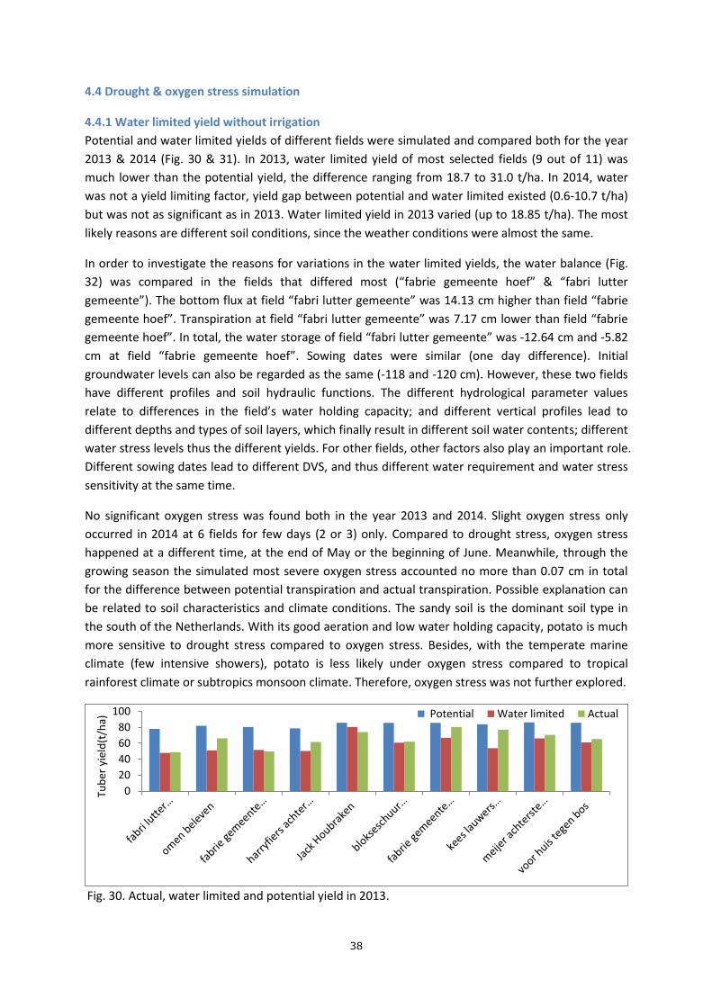
4.4.1 Water limited yield without irrigation

Potential and water limited yields of different fields were simulated and compared both for the year

2013 & 2014 (Fig. 30 & 31). In 2013, water limited yield of most selected fields (9 out of 11) was

much lower than the potential yield, the difference ranging from 18.7 to 31.0 t/ha. In 2014, water

was not a yield limiting factor, yield gap between potential and water limited existed (0.6-10.7 t/ha)

but was not as significant as in 2013. Water limited yield in 2013 varied (up to 18.85 t/ha). The most

likely reasons are different soil conditions, since the weather conditions were almost the same.

In order to investigate the reasons for variations in the water limited yields, the water balance (Fig.

32) was compared in the fields that differed most (“fabrie gemeente hoef” & “fabri lutter

gemeente”). The bottom flux at field “fabri lutter gemeente” was 14.13 cm higher than field “fabrie

gemeente hoef”. Transpiration at field “fabri lutter gemeente” was 7.17 cm lower than field “fabrie

gemeente hoef”. In total, the water storage of field “fabri lutter gemeente” was -12.64 cm and -5.82

cm at field “fabrie gemeente hoef”. Sowing dates were similar (one day difference). Initial

groundwater levels can also be regarded as the same (-118 and -120 cm). However, these two fields

have different profiles and soil hydraulic functions. The different hydrological parameter values

relate to differences in the field’s water holding capacity; and different vertical profiles lead to

different depths and types of soil layers, which finally result in different soil water contents; different

water stress levels thus the different yields. For other fields, other factors also play an important role.

Different sowing dates lead to different DVS, and thus different water requirement and water stress

sensitivity at the same time.

No significant oxygen stress was found both in the year 2013 and 2014. Slight oxygen stress only

occurred in 2014 at 6 fields for few days (2 or 3) only. Compared to drought stress, oxygen stress

happened at a different time, at the end of May or the beginning of June. Meanwhile, through the

growing season the simulated most severe oxygen stress accounted no more than 0.07 cm in total

for the difference between potential transpiration and actual transpiration. Possible explanation can

be related to soil characteristics and climate conditions. The sandy soil is the dominant soil type in

the south of the Netherlands. With its good aeration and low water holding capacity, potato is much

more sensitive to drought stress compared to oxygen stress. Besides, with the temperate marine

climate (few intensive showers), potato is less likely under oxygen stress compared to tropical

rainforest climate or subtropics monsoon climate. Therefore, oxygen stress was not further explored.

Fig. 30. Actual, water limited and potential yield in 2013.

0

20

40

60

80

100

Tub

er y

ield

(t/h

a) Potential Water limited Actual

39

Fig. 31. Actual, water limited and potential yield in 2014.

Fig. 32. Water balance of field “fabri lutter gemeente” (left) and “fabrie gemeente hoef” (right) in

2013.

4.4.2 Sensitivity analysis of pressure head and underground water level

Only one value of H1, H2, H3l, H3h, H4 was changed with ±1% at each time. Results showed that water

limited yields with different h values were remain same. Considering field “fabri lutter gemeente” in

2013 was already under severe drought stress conditions, 1% changing of h values could have little

impact on water limited yield. So a new sensitivity analysis with 10% change of h values was tested at

each time. Results are as same as previous only slightly difference by changing H4 values but it can be

neglected. In order to make the sensitivity analysis more representative, other three fields: “wauters

achter stal”, “v.d. sande naast schuur” in 2014 and “fabrie gemeente hoef” in 2013 were also

performed with sensitivity analysis. Field “fabrie gemeente hoef” in 2013 were under middle

drought stress level, while there were no drought stress in fields “wauters achter stal”, “v.d. sande

naast schuur” in 2014. With 1 % changing of values of h1, h2, h3h ,h3l and h4, yield remained same

for the fields in 2014. Simulated actual yield was found negatively related to h4 value in field “fabrie

gemeente hoef” in 2013. But simulated Ya only increased 24 kg/ha with h4 value increased from

9600 to 10400, which can be ignored. Reason to explain the results is that with the same simulated h

value, a predefined lower h4 value result in a higher αrw value which means less drought stress and

higher yield. Since only the value of h4 has impact on Yw while the field in under drought stress,

more tests were done with the continuing increasing h4 value for field “fabrie gemeente hoef” in

2013 . Simulated yield was found gradually decreased. In short conclusion, finding the wilting point

where the h4 value located is crucial for precise drought stress simulation. Based on the sensitivity

0

20

40

60

80

100

120

Tub

er y

ield

(t/h

a)

Potential Water limited Actual

40

analysis results, default h values would be used for water stress simulation. But experiment was

recommended to detect the wilting point in the future.

In “fabri lutter gemeente”, no influential oxygen stress was found on the farm in both two years, the

effect of another factor was investigated, underground water level (UWL) (Fig. 33). Yw is positively

related to UWL in 2013. And it appears that Yw is not sensitive to the UWL in 2014. Possible reason

to explain the different effects of underground water levels on Yw is related to the accumulated

precipitation during the summer. Yw in 2013 of the two fields were under drought stress during the

summer because of the deficiency of rainfall, thus the Yw of fields with low soil moisture content

were more sensitive to UWL. In terms of the fields in 2014, yield of field “wauters achter stal” was at

optimal level. With sufficient rainfall and good water holding capacity, Yw was not sensitive to UWL.

However, field “v.d. sande naast schuur” was also under drought stress during the Julian days of mid

to the end of June, which was the tuber initiation stage. But in the followed summer season, large

amount of rainfall ensured desirable soil moisture maintained during the tuber filling stage.

Therefore, UWL was of sub-importance and Yw was less sensitive to it compared to the fields in 2013.

Fig. 33. Effects of underground water levels on water limited yield.

4.4.3 Evapotranspiration & soil water content

As the field “fabri lutter gemeente” had the lowest water limited yield in 2013, evapotranspiration is

presented (Fig. 34). Potential transpiration was much higher (0-5.0 cm per day) than the actual

during the most of the period from Julian day 190 to 250. Potential soil evaporation was higher (0-1.7

mm per day) than the actual during Julian day 50-165 and some days around 250, and also most days

between 264-294. Drought stress (0-5.4 mm per day) occurred since Julian day 192 until 252.

Drought stress peaks arose at days 197, 203, 228 and 248 (Fig. 36). Soil volumetric water content in

the depth of 0-50 cm was low (under 0.15) since day 190.

-8

-6

-4

-2

0

2

4

6

8

10

12

-50 -40 -30 -20 -10 0 10 20 30 40 50

Yw changed (%)

Underground water levels changed (cm)

2013 fabri lutter gemeente 2013 fabrie gemeente hoef

2014 v.d. sande naast schuur 2014 wauters achter stal

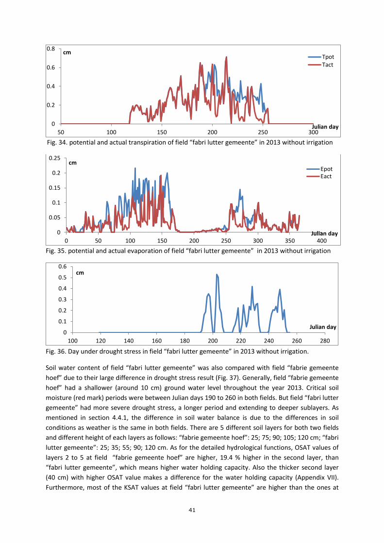
41

Fig. 34. potential and actual transpiration of field “fabri lutter gemeente” in 2013 without irrigation

Fig. 35. potential and actual evaporation of field “fabri lutter gemeente” in 2013 without irrigation

Fig. 36. Day under drought stress in field “fabri lutter gemeente” in 2013 without irrigation.

Soil water content of field “fabri lutter gemeente” was also compared with field “fabrie gemeente

hoef” due to their large difference in drought stress result (Fig. 37). Generally, field “fabrie gemeente

hoef” had a shallower (around 10 cm) ground water level throughout the year 2013. Critical soil

moisture (red mark) periods were between Julian days 190 to 260 in both fields. But field “fabri lutter

gemeente” had more severe drought stress, a longer period and extending to deeper sublayers. As

mentioned in section 4.4.1, the difference in soil water balance is due to the differences in soil

conditions as weather is the same in both fields. There are 5 different soil layers for both two fields

and different height of each layers as follows: “fabrie gemeente hoef”: 25; 75; 90; 105; 120 cm; “fabri

lutter gemeente”: 25; 35; 55; 90; 120 cm. As for the detailed hydrological functions, OSAT values of

layers 2 to 5 at field “fabrie gemeente hoef” are higher, 19.4 % higher in the second layer, than

“fabri lutter gemeente”, which means higher water holding capacity. Also the thicker second layer

(40 cm) with higher OSAT value makes a difference for the water holding capacity (Appendix VII).

Furthermore, most of the KSAT values at field “fabri lutter gemeente” are higher than the ones at

0

0.2

0.4

0.6

0.8

50 100 150 200 250 300

cm

Julian day

TpotTact

0

0.05

0.1

0.15

0.2

0.25

0 50 100 150 200 250 300 350 400

cm

Julian day

EpotEact

0

0.1

0.2

0.3

0.4

0.5

0.6

100 120 140 160 180 200 220 240 260 280

cm

Julian day

42

field “fabrie gemeente hoef”. According to Neumann’s condition, higher KSAT values result in a

higher bottom flux (14.13 cm), and thus less available water stored in the upper layers.

Fig. 37. Soil water content of field “fabri lutter gemeente” (left) and “fabrie gemeente hoef” (right) in

the year 2013.

4.4.4 The impact of rainfall and soil type on drought stress

Severe drought stress was found in several potato fields in the year 2013 and the stress level varied

among them (Fig. 30). There are two main reasons behind the different levels of drought stress at

different fields. The first reason is the difference in rainfall inputs. Two weather stations with

recorded rainfall data from Dacom were used. Between these two stations (4 km in distance) rainfall

data varied (Fig. 38). There were 3 peaks of rainfall recorded between days 191 to 217 at field “Cor

weg eersel”. In order to test the influence of these two different rainfall data on drought stress, field

“fabri lutter gemeente” was simulated twice with different sets of rainfall data. Significant different

water limited yield was obtained in the model. DM yield of 8531 Kg/ha and 13120 Kg/ha were

simulated with weather input from location “blokseschuur tegen bos” (BTB) and “cor weg eersel”

(CWE) respectively. Drought stress was compared between the two simulations (Fig. 39). Simulation

with BTB rainfall inputs suffered longer (more than one month) and more severe drought stress (67

mm higher in total). Therefore, the variability of rainfall data has direct and strong influence on the

drought stress results and water limited yield simulation. In order to achieve most precise and

reliable simulations, high quality rainfall data are essential and weather data sources should be

cautiously selected.

Fig. 38. Recorded rainfall in 2013 for two different locations

0

10

20

30

40

50

60

120 140 160 180 200 220 240 260 280 300 320

Rai

nfa

ll (m

m)

blokseschuur tegen bos

cor weg eersel

43

Fig. 39. Drought stress of field “fabri lutter gemeente” with different rainfall inputs

In order to quantify the influence of different soil profiles on the water limited yield, a sensitivity

analysis using Eindhoven weather data was done (Fig. 40). There were 15 different soil profiles used

in the simulation. Growing period and ground water level were the same for the same year. In the

year 2013, simulated water limited yield differed with a range of 0-26.4 t/ha due to the different soil

profile inputs. As for the year 2014, the range was smaller with 0-9.4 t/ha. In the context of the same

year, water limited yield is sensitive to the soil profile inputs. In the context of different years,

besides other factors water limited yield was determined by the rainfall firstly, and then the soil

inputs.

Fig. 40. Simulated water limited yield based on same weather inputs (Eindhoven) for different soil

type (DM content 18 %). Detailed information related to soil codes can be found in Appendix IV

As for the difference between the years, water limited yields in year 2014 were more than 20 t/ha

and up to 45 t/ha higher than in 2013. Total rainfall in 2013 recorded at Eindhoven was 704.35 mm

whereas in 2014 it was 805.7 mm. Moreover, the distribution of rainfall was also different in these

two years (Fig. 3), especially in July and August. During these two months, precipitation was 80.4 mm

in 2013 and 301 mm in 2014. Most potato fields were sown in April in both years (one month sowing

window), and tuber initiation started at the end of June and beginning of July. The dry period during

filling stage largely accounted for the severe yield loss in 2013.

0

0.1

0.2

0.3

0.4

0.5

0.6

170 180 190 200 210 220 230 240 250 260

Dro

ugh

t st

ress

(cm

) blokseschuur tegen bos

cor weg eersel

0

20

40

60

80

100

301 302 303 304 305 306 310 311 312 313 314 317 318 321 324

Yiel

d (

t/h

a)

Soil code

Water limited yield 2014 water limited yield 2013

44

4.4.5 Simulation with irrigation

Accumulative WSO was simulated with and without model scheduled irrigation. Observed WSO in

the field “fabri lutter gemeente” was compared with the simulated WSO of the two different

scenarios (Fig. 45). Between the two simulated WSO, a 5742 Kg/ha higher DM yield was obtained

with the automatic irrigation. The first two irrigations eliminate the early drought stress and enable

unlimited tuber initiation and linearly primary tuber growth. The third and fourth irrigation were

applied at the middle stage of tuber growth, which was the most severe drought stress period.

Without irrigation, tuber growing speed decreased sharply after the first drought stress day (192).

Actual WSO was observed four times at Julian day 205, 218, 231 and 255. In general, three (except

the second one) out of four observations had a similar growing trend with the simulation without

irrigation, and WSO values as well. However, the second observed WSO was much higher than the

two simulations, 6501 kg/ha higher than the non-irrigated simulation and 4505 Kg/ha higher than the

irrigated one, which is abnormal and interesting to investigate. One of the possible reasons is that

this point is simply an outlier. By checking the UWW of the second observation, a UWW value of 505

was recorded whereas an average of 318 was calculated at farm level. The extreme high UWW leads

to the high DM content (28.05 % at second observation pint), whereas a DM of 17.67 % was obtained

with the average UWW (318).

Fig. 45. Modelling accumulative water limited WSO with & without irrigation also the observed WSO

of field “fabri lutter gemeente” in 2013.

In order to estimate the required irrigation, an automatic irrigation schedule using the critical

pressure head criterial was generated in SWAP-WOFOST (Fig. 41). Drought stress was eliminated with

irrigation. The yield gap caused by water stress was closed in 2013 for all of the selected fields. As for

year the 2014, the yield gap between potential and water limited can be neglected, only 1 to 2 t/ha

existed for three fields. As for the field “fabri lutter gemeente” in 2013, irrigation generated by the

model was applied 5 times and at a dose of 4.3 cm each time. With irrigation, actual transpiration

was increased to potential. Actual evaporation remained the same (Fig. 42 & 43). Irrigation was

4.05

4.1

4.15

4.2

4.25

4.3

4.35

4.4

4.45

4.5

4.55

0

2000

4000

6000

8000

10000

12000

14000

16000

150 170 190 210 230 250 270

TWSO (kg/ha)

Day

TWSO without irrigation

TWSO with irrigation

OB TWSO

Irrigation by model

Irrigation (cm)

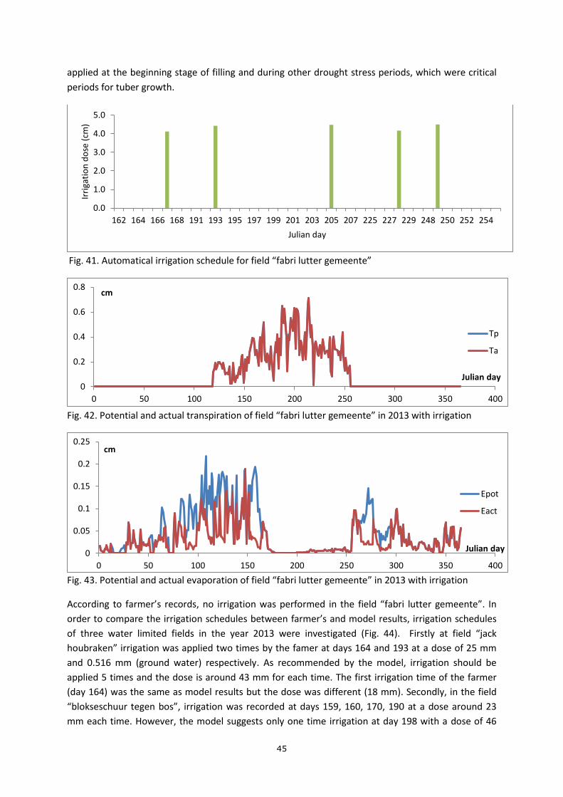
45

applied at the beginning stage of filling and during other drought stress periods, which were critical

periods for tuber growth.

Fig. 41. Automatical irrigation schedule for field “fabri lutter gemeente”

Fig. 42. Potential and actual transpiration of field “fabri lutter gemeente” in 2013 with irrigation

Fig. 43. Potential and actual evaporation of field “fabri lutter gemeente” in 2013 with irrigation

According to farmer’s records, no irrigation was performed in the field “fabri lutter gemeente”. In

order to compare the irrigation schedules between farmer’s and model results, irrigation schedules

of three water limited fields in the year 2013 were investigated (Fig. 44). Firstly at field “jack

houbraken” irrigation was applied two times by the famer at days 164 and 193 at a dose of 25 mm

and 0.516 mm (ground water) respectively. As recommended by the model, irrigation should be

applied 5 times and the dose is around 43 mm for each time. The first irrigation time of the farmer

(day 164) was the same as model results but the dose was different (18 mm). Secondly, in the field

“blokseschuur tegen bos”, irrigation was recorded at days 159, 160, 170, 190 at a dose around 23

mm each time. However, the model suggests only one time irrigation at day 198 with a dose of 46

0.0

1.0

2.0

3.0

4.0

5.0

162 164 166 168 191 193 195 197 199 201 203 205 207 225 227 229 248 250 252 254

Irri

gati

on

do

se (

cm)

Julian day

0

0.2

0.4

0.6

0.8

0 50 100 150 200 250 300 350 400

cm

Julian day

Tp

Ta

0

0.05

0.1

0.15

0.2

0.25

0 50 100 150 200 250 300 350 400

cm

Julian day

Epot

Eact

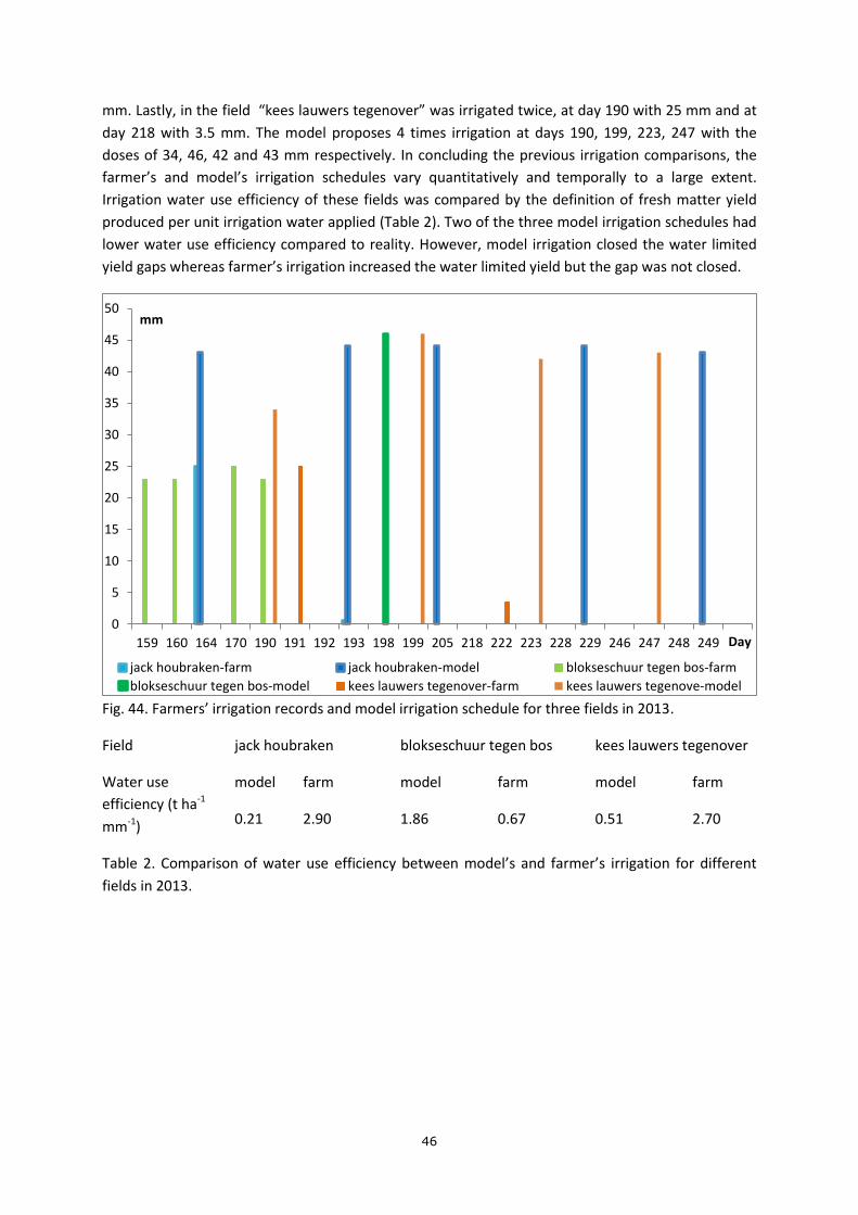
46

mm. Lastly, in the field “kees lauwers tegenover” was irrigated twice, at day 190 with 25 mm and at

day 218 with 3.5 mm. The model proposes 4 times irrigation at days 190, 199, 223, 247 with the

doses of 34, 46, 42 and 43 mm respectively. In concluding the previous irrigation comparisons, the

farmer’s and model’s irrigation schedules vary quantitatively and temporally to a large extent.

Irrigation water use efficiency of these fields was compared by the definition of fresh matter yield

produced per unit irrigation water applied (Table 2). Two of the three model irrigation schedules had

lower water use efficiency compared to reality. However, model irrigation closed the water limited

yield gaps whereas farmer’s irrigation increased the water limited yield but the gap was not closed.

Fig. 44. Farmers’ irrigation records and model irrigation schedule for three fields in 2013.

Field jack houbraken blokseschuur tegen bos kees lauwers tegenover

Water use

efficiency (t ha-1

mm-1)

model farm model farm model farm

0.21 2.90 1.86 0.67 0.51 2.70

Table 2. Comparison of water use efficiency between model’s and farmer’s irrigation for different

fields in 2013.

0

5

10

15

20

25

30

35

40

45

50

159 160 164 170 190 191 192 193 198 199 205 218 222 223 228 229 246 247 248 249

mm

Day

jack houbraken-farm jack houbraken-model blokseschuur tegen bos-farm

blokseschuur tegen bos-model kees lauwers tegenover-farm kees lauwers tegenove-model

47

5. Discussion

5.1 WOFOST calibration and validation for potential yield simulation

The WOFOST calibration was done for potential yield calibration because model parameters values

were obtained at field experiments more than 20 years ago (Boons-Prins et al. 1993). The calibration

data were based on the farmer’s phenology records and tuber yields at different times during the

growing season. Potential yields after calibration reached 88-94 t/ha in 2014 and 78-86 t/ha in 2013,

with a DM of 18 %. However, the highest yield obtained at the farm was 100 t/ha in 2014 and 95 t/ha

in 2013, several tons higher than the simulation results, which was not desirable. The reason is that

model calibration was based on a series of fields with highest yield whereas the yield of 100 t/ha and

95 t/ha were from one field.

Highest yield achieved at field level cannot equal to farm level. According to Lobell et al. (2009), the

exploitable yield is 80 % of potential yield on a national scale. If the highest yield in the farm is

considered as exploitable, potential yield of cultivar Fontane should be increased 20 % which is

105.6-112.8 t/ha in 2014 and 93.6-103.2 in 2013. The differences in simulated potential yields

between the two years were 9.6-12 t/ha. The cultivars Miranda, Ludmilla and Lady Anna were also

planted in several fields, however, due to their small scale and relatively lower yield compared to

Fontane, no calibration was performed, and potential yields for these three cultivars could not be

determined.

Even though the model efficiency was higher than 0.9 for most of the fields at the validation (Figure

28), model uncertainty cannot be neglected. At the step of CO2 assimilation parameter AMAXTB

calibration, a contradictory condition occurred between the phenology parameter TSUM1 and

observed anthesis date. The TSUM1 value was reset from the calibrated value (420 ℃) to 320 ℃ at this

step in order to match the observed accumulative WSO. TSUM1 was changed with 100 ℃ from the

calibrated value, which was not desired. A possible reason could be that the observed anthesis date,

which was obtained indirectly from pictures, was incorrect.

Besides parameter TSUM1, another issue of model uncertainty is related to the observed data of

WSO. WSO is the key indicator at the AMAXTB calibration, however, within the selected fields for

calibration, sowing dates were different, as well as WSO measuring dates and the UWW.

Heterogeneous WSO data were averaged (sowing date & measurement data) for calibration,

however, the simplified procedure could also cause model uncertainty. Simply averaging all the data

results in underestimated potential yield to the mean level within these fields. This is why the

simulated potential yield is lower than the observed highest yield in both of two years for some fields.

Moreover, not all of the parameters suggested by the Wolf (2003) were calibrated due to

unavailability of data. These parameters include SLATB, FSTB, FOTB and FLTB. Model calibration can

be improved with additional data.

Moreover, WOFOST underestimated the potential yield at fields “vermeulen hulsel”, “mark

hurkmans” and “wauters achter stal” in 2013 (Fig. 26). These three fields had highest yields with

non-linearly accumulated tuber mass growing tendency (Fig.11), whereas WOFOST calibration was

based on the criterial of selecting data from fields with linearly increasing tuber growth trend. The

48

underestimation results should be further investigated with experiments under potential production

conditions.

5.2 Water limited yield simulation

According to the simulation results, farm Van den Borne Aardappelen suffered severe drought stress

in the year 2013 which caused 18.7 to 31.0 t/ha yield loss. In contrast, in the year 2014 no significant

yield loss was caused by drought, and the average yield obtained in 2014 was 10 t/ha higher than

2013. However, no drought stress or oxygen stress experiment was designed and performed in the

farm, thus simulated water limited yield cannot be quantitatively validated by reality. It is unclear

whether the model can simulate drought and oxygen stress adequately in the context of observed

water limited yield. In order to evaluate model performance for water stress simulation, an indirect

assessment by comparing Dacom soil moisture data and model results was done. The soil moisture

data in 2014 at different soil depths of field “Jan luiksgestel achter bos” was compared (Appendix

VIII), because the rainfall was measured at this field and soil moisture data are available. Observed

soil moisture value was much higher at all the different depths compared to the simulation results,

but they have a similar trend. According to the soil map from Wösten et al. (2012), saturated soil

water content at this field is 0.43 cm3/cm3 for the first layer and 0.36 cm3/cm3 for the sublayers. The

topsoil layer is 8.0 cm deep and the rest are 215 cm. As for observation, soil moisture was higher

than 0.5 cm-3/cm-3 at the depth of 10 cm for most of the days after 8th of July, which is even higher

than the saturated value. Similarly, soil moisture at other depths were also relatively high.

It may be that the Dacom soil moisture sensor was not calibrated before measuring. Thus, using the

soil moisture data of this field is risky and model simulated water content can only compared with

measurements in a relative sense. The model performance assessment was aborted due to

anomalous high soil water content data. There are however also other possible explanations for the

differences between observed and simulated soil water contents. The soil map of Wösten et al. (2012)

was made years before. During the years of soil management (e.g. fertilization & tillage), soil

properties (soil hydraulic functions & top boundary condition) could already have changed, causing

the big difference between the simulations and observations. The theory behind is that the changes

of soil hydraulic functions and the top boundary conditions have significant influence on the

simulated phreatic surface fluctuations at shallow groundwater tables (Van Dam et al., 2008).

Meanwhile, another possibility is that SWAP performed poor in this field without calibration. In order

to inspect this issue, further experiments and research are required, for instance detecting the soil

hydrological properties and calibrating SWAP.

As for the oxygen stress, underground water levels for all the fields in these two years were far more

below the root zone (30 cm in all simulations). Underground water levels were found at the depths

around 100cm in the study area, which was not able to cause waterlogging problem. However, based

on the opinion of the farmer and literature, 30 cm of the maximum rooting depth was used in all the

simulations without collecting data at fields. Further studies can investigate the influences of deeper

or shallower rooting depth on oxygen stress or drought stress level. Besides, potato waterlogging

problem (oxygen stress) is less likely occurred under temperate marine climate conditions with sandy

soil. High quality of soil moisture data are required if water stress (drought & oxygen) will be further

investigated.

49

Four among the 10 observed actual yields in 2013 were much higher (up to 23 t/ha) than the

simulated water limited yield. A possible reason is that the actual yield is achieved with applied

irrigation, and thus the yield gap due to water stress is closed to some extent. The irrigated fields

were “blokseschuur tegen bos” and “kees lauwers tegenover”. While in the latter one, actual yield

was indeed much higher than water limited yield , in the first one they were similar. Another reason

could be that the model has not been calibrated for water limited yield, and the model overestimates

yield gaps caused by water. Another reason could be that the weather input, especially in

precipitation data were not accurate enough for some fields. Other reasons could be the pests,

diseases and weeds are not included in the model. While in 2013, water limitation seems to play a

major role in the actual yields, in 2014 water was not the crucial constraint and the yield gaps is

caused by these later other factors.

Previous studies also found that drought stress on potato tuber initiation and filling stages have the

most significant effect on yield (MacKerron and Jefferies, 1986; Haverkort et al., 1990; Lynch et al.,

1995; Yuan et al., 2003). Moreover, most drought stress periods were also found during July and

August. Maximum rooting depth in all the simulations was assumed to be 30 cm. In principle this

value should be adjusted to match different situation in different fields. However, it is unfeasible

without relevant data. Thus, 30 cm was used based on the farmer’s opinion and literature (Opena &

Porter, 1999). Another uncertainty relates to the groundwater level data. Not all of the groundwater

data were measured right on the fields. Some of them were even hundreds meters away from the

field. These two uncertainties can be solved by improved data collection.

5.4 Implement SWAP-WOFOST for irrigation schedule

The main purpose of this study was to understand to what extent drought reduced yield in the years

2013 and 2014. A sub-aim was to provide a solution by implementing SWAP-WOFOST to achieve

better water management in order to close the yield gap. There are currently different ways for

agricultural water management. One of them is using drainage. Different scenarios of drainage water

management can be applied at different periods for different purposes (Fig. 46). The outlets can be

raised after harvest to reduce nitrate leaching, lowered in early spring and fall to allow free drainage

before planting or harvest, or raised after planting to increase soil water content for the summer

(Frankenberger et al,. 2004). However, this method is expensive and time consuming for

infrastructure construction, while the farm has unfixed and a large amount of fields, so this type of

drainage management is not economically efficient.

Fig. 46. Drainage water management at different periods, after harvest (a); early spring and fall (b);

after planting (c) (Frankenberger et al., 2004)

a b c

50

Another water management method is using drip irrigation, but drip irrigation is most suitable for

row crops, trees and vine crops. A drip system further requires high investment, which is also not a

desirable choice. Thus the solution should meet the requirements of being time efficient, inexpensive

and suitable. A Modelling approach is then considered.

Since one of the functions of a model is prediction, SWAP-WOFOST can be used for soil moisture

estimation. Based on the soil moisture conditions, an irrigation schedule can be generated from the

model with a certain dose and time for application. In order to make an irrigation schedule,

prediction of weather in a certain period is pre-required. At the same time, for the purpose of precise

estimations, SWAP should be calibrated before implementation. If the predicted weather data is 14

days available in advance, this would be a great advantage for scheduling irrigation. At the same time,

the model irrigation schedule highly depends on the weather prediction. 14 days would allow the

farmer to have more time to plan irrigation management in the context of the large scale of the farm

and saving time for other farm operations. However, in case weather forecasting is not available,

SWAP-WOFOST can also use currently measured weather data to estimate soil water condition and

give irrigation advice. Since Van den Borne is a large scale precision farm, and spatial variability in

water management exists, one of the solutions could be using GIS to assist irrigation. Fortes et al.

(2005) integrated GIS with the irrigation scheduling simulation model ISAREG to improve water usage

in Uzbekistan. The integrated model GISAREG was applied to assess alternative irrigation scenarios.

GIS enables the model to be more applicable for a large scale area. Moreover, the clear overview

distribution of spatial water demand can be visualized with the assistance of GIS. The various water

managements at the farm or regional level can also be localized, and can thus support further

analysis of water and irrigation requirements. Therefore, combing SWAP-WOFOST and GIS will be a

useful tool for the irrigation scheduling and preferably with predicting weather data.

51

6. Conclusions & Recommendations

The aim of this study was to evaluate the impact of drought and oxygen stress on potato yield and

improve water management. The following conclusions can be derived:

Potential fresh yield of potato cultivar Fontane was determined at the farm with a range of

90-120 t/ha, depending on the growing period and weather.

While simulated potential yields with WOFOST were far below the observed levels with

default parameters, calibration result in yields similar to observations in the highest yielding

fields. Exact calibration however requires experiments.

Simulated yield gap caused by water was 18.7 to 31.0 t/ha in 2013 and 0.6-10.7 t/ha in 2014.

Results of water limited yield simulations however cannot be verified with the current

database.

In 2013, the farm was found under severe drought stress for a long period (more than 30

days). Slight oxygen stress was found for both years, but has insignificant effect on yield.

Potato water limited yield is highly influenced by the level of water stress during the tuber

initiation and filling stage. Farm management should focus more on fields water states

during summer.

Data used for crop model calibration should be carefully selected and the reliability of the

data are essential, as these have a direct influence on model outputs. Within them, the

phenology data and tuber yield data were most crucial.

Potential yield can be well simulated by SWAP-WOFOST after calibration at the large scale

farm.

Sufficient data are required for model application. High resolution of soil data and accurate

precipitation data are two of the most important inputs for water limited yield simulation.

Without experiments performed in reality considering water stress, It is impossible to

validate model results which leave a huge uncertainty of the reliability of model performance.

Whether SWAP-WOFOST can adequately simulate drought-or oxygen stress cannot be

determined in this case study. Further experiments and studies are required to answer this

question.

Researches such as the soil map from Wösten et al. (2012) can provide essential information

to support the application of SWAP-WOFOST, but the accuracy of the data should be checked

with additional lab work.

SWAP-WOFOST can efficiently improve water management in terms of irrigation scheduling

and lead to higher yield.

Detailed weather prediction for a short period can enhance model application for irrigation

A modeling approach should be integrated with GIS in terms of large scale precision farm to

achieve higher yield.

As for yield gap analysis, future studies should include more yield affecting factors into the

modelling approach. A whole system approach including water, nutrients, pests,

management and diseases should be developed and applied.

52

Reference Ashraf, M., & Mehmood, S. (1990). Effects of waterlogging on growth and some physiological

parameters of four Brassica species. Plant and Soil, 121(2), 203-209.

Bartholomeus, R. P., Witte, J. P. M., Van Bodegom, P. M., van Dam, J. C., & Aerts, R. (2008). Critical

soil conditions for oxygen stress to plant roots: Substituting the Feddes-function by a process-based

model. Journal of Hydrology, 360(1), 147-165.

Bhatia, V. S., Singh, P., Wani, S. P., Chauhan, G. S., Rao, A. K., Mishra, A. K., & Srinivas, K. (2008).

Analysis of potential yields and yield gaps of rainfed soybean in India using CROPGRO-Soybean model.

Agricultural and Forest Meteorology, 148(8), 1252-1265.

Boogaard, H.L., De Wit, A.J.W., Te Roller, J.A., Van Diepen, C.A. (2014) User’s guide for the WOFOST

Control Centre 2.1 and WOFOST 7.1.7 crop growth simulation model. Alterra Wageningen UR.

Boon-Prins, E. R. (1993). Crop-specific simulation parameters for yield forecasting across the

European Community. Simulation Reports AB-TPE, no. 32, AB-DLO, Wageningen.

Boote, K. J., Jones, J. W., & Pickering, N. B. (1996). Potential uses and limitations of crop models.

Agronomy Journal, 88(5), 704-716.

Braden, H., 1985. Ein Energiehaushalts- und Verdunstungsmodell for Wasser und Stoffhaushaltsuntersuchungen landwirtschaftlich genutzer Einzugsgebiete. Mittelungen Deutsche Bodenkundliche Geselschaft, 42, 294-299. Dalla Costa, L., Delle Vedove, G., Gianquinto, G., Giovanardi, R., & Peressotti, A. (1997). Yield, water use efficiency and nitrogen uptake in potato: influence of drought stress. Potato Research, 40(1), 19-34. DESA, U. (2013). World Population Prospects, The 2012 Revision. New York: Department for Economic and Social Affairs. De Wilde, T., De Meulenaer, B., Mestdagh, F., Govaert, Y., Ooghe, W., Fraselle, S., ... & Verhé, R.

(2006). Selection criteria for potato tubers to minimize acrylamide formation during frying. Journal of

agricultural and food chemistry, 54(6), 2199-2205.

Else, M. A., Davies, W. J., Malone, M., & Jackson, M. B. (1995). A negative hydraulic message from

oxygen-deficient roots of tomato plants? (influence of soil flooding on leaf water potential, leaf

expansion, and synchrony between stomatal conductance and root hydraulic conductivity). Plant

Physiology, 109(3), 1017-1024.

Feddes, R. A., Kowalik, P. J., & Zaradny, H. (1978). Simulation of field water use and crop yield. Centre

for Agricultural Publishing and Documentation.

Fortes, P. S., Platonov, A. E., & Pereira, L. S. (2005). GISAREG—A GIS based irrigation scheduling

simulation model to support improved water use. Agricultural Water Management, 77(1), 159-179.

Frankenberger, J., Kladivko, E., Sands, G., Jaynes, D. B., Fausey, N., Helmers, M. J., Cooke, R., Strock, J., Nelson, K., Brown, L. C. (2004). Drainage water management for the midwest. https://www.extension.purdue.edu/extmedia/wq/wq-44.pdf

53

Goudriaan, J., 1986. A simple and fast numerical method for the computation of daily crop photosynthesis. Agricultural and Forest Meteorology 38: 249-254. Haverkort, A. J., Van de Waart, M., & Bodlaender, K. D. (1990). The effect of early drought stress on numbers of tubers and stolons of potato in controlled and field conditions. Potato Research, 33(1), 89-96. Hedden, P. (2003). The genes of the Green Revolution. Trends in Genetics, 19(1), 5-9. H.L. Boogaard., A.J.W. De Wit., J.A. te Roller., C.A. Van Diepen., R.P. Rötter., J.M.C.A. Cabrera., H.H.

Van Laar. (2014). User’s guide for the WOFOST Control Centre 2.1 and WOFOST 7.1.7 crop growth

simulation model. Alterra, Wageningen University & Research Centre.

Holtman, W. L., Oppedijk, B. J., Vennik, M., & van Duijn, B. (2014). Low Oxygen Stress in Horticultural

Practice. In Low-Oxygen Stress in Plants (pp. 371-380). Springer Vienna.

http://precisielandbouw.eu/pplnl/Home.html http://www.vandenborneaardappelen.com.html Ines, A. V. M., Makin, P., & IW Das Gupta, A. (2001). Crop growth and soil water balance modeling to

explore water management options (Vol. 22).

http://www.iwmi.cgiar.org/Publications/Working_Papers/working/WOR22.pdf

Karafyllidis, D. I., Stavropoulos, N., & Georgakis, D. (1996). The effect of water stress on the yielding

capacity of potato crops and subsequent performance of seed tubers. Potato research, 39(1), 153-

163.

Licker, R., Johnston, M., Foley, J. A., Barford, C., Kucharik, C. J., Monfreda, C., & Ramankutty, N. (2010). Mind the gap: how do climate and agricultural management explain the ‘yield gap’of croplands around the world?. Global Ecology and Biogeography, 19(6), 769-782. Lobell, D. B., Cassman, K. G., & Field, C. B. (2009). Crop yield gaps: their importance, magnitudes, and causes. Annual Review of Environment and Resources, 34(1), 179. Lynch, D. R., Foroud, N., Kozub, G. C., & Fames, B. C. (1995). The effect of moisture stress at three growth stages on the yield, components of yield and processing quality of eight potato varieties. American Potato Journal, 72(6), 375-385. MacKerron, D. K. L., & Jefferies, R. A. (1986). The influence of early soil moisture stress on tuber

numbers in potato. Potato Research, 29(3), 299-312.

Neumann, K., Verburg, P. H., Stehfest, E., & Müller, C. (2010). The yield gap of global grain production: A spatial analysis. Agricultural Systems, 103(5), 316-326. Ojala, J. C., Stark, J. C., & Kleinkopf, G. E. (1990). Influence of irrigation and nitrogen management on

potato yield and quality. American Potato Journal, 67(1), 29-43.

Opena, G. B., & Porter, G. A. (1999). Soil management and supplemental irrigation effects on potato:

II. Root growth. Agronomy Journal, 91(3), 426-431.

54

Penning de Vries, F.W.T., 1975. The cost of maintenance processes in plant cells. Annals of Botany

39:77-92.

Penning de Vries, F.W.T, D.M. Jansen, H.F.M. ten Berge and A. Bakema, 1989. Simulation of

ecophysiological processes of growth in several annual crops. Simulation Monographs 29. Pudoc,

Wageningen.

Prost, L., Makowski, D., & Jeuffroy, M. H. (2008). Comparison of stepwise selection and Bayesian

model averaging for yield gap analysis. Ecological Modelling, 219(1), 66-76.

Reidsma, P., Descheemaeker, K., Bianchi, F., Lubbers, M., Allema, B., Vargas, V. D. (2012). Systems

analysis, Simulation and Systems Management PPS 20306. Alterra Wageningen UR.

Reidsma, P., Wolf, J., Kanellopoulos, A., Schaap, B. F., Mandryk, M., Verhagen, J., & van Ittersum, M.

K. (2015). Climate change impact and adaptation research requires integrated assessment and

farming systems analysis: a case study in the Netherlands. Environmental Research Letters, 10(4),

045004.

Rijk, B., van Ittersum, M., & Withagen, J. (2013). Genetic progress in Dutch crop yields. Field Crops

Research, 149, 262-268.

Seelan, S. K., Laguette, S., Casady, G. M., & Seielstad, G. A. (2003). Remote sensing applications for

precision agriculture: A learning community approach. Remote Sensing of Environment, 88(1), 157-

169.

Spitters, C. J. T., Keulen, H. V., & Van Kraalingen, D. W. G. (1989). A simple and universal crop growth

simulator: SUCROS87. http://edepot.wur.nl/171923.

UN, D. (2013). World Population Prospects: The 2012 Revision.

http://esa.un.org/wpp/Documentation/pdf/WPP2012_%20KEY%20FINDINGS.pdf

Van Dam, J. C., Groenendijk, P., Hendriks, R. F., & Kroes, J. G. (2008). Advances of modeling water

flow in variably saturated soils with SWAP. Vadose Zone Journal, 7(2), 640-653.

Van Dam, J. C., Groenendijk, P., Hendriks, R. F. A., & Jacobs, C. M. J. (2008). SWAP version 3.2: Theory

description and user manual. Wageningen, The Netherlands: Alterra.

Van Loon, C. D. (1981). The effect of water stress on potato growth, development, and yield.

American Potato Journal, 58(1), 51-69.

Van Ittersum, M. K., Cassman, K. G., Grassini, P., Wolf, J., Tittonell, P., & Hochman, Z. (2013). Yield gap analysis with local to global relevance—a review. Field Crops Research, 143, 4-17. Van Ittersum, M. K., & Rabbinge, R. (1997). Concepts in production ecology for analysis and

quantification of agricultural input-output combinations. Field Crops Research, 52(3), 197-208.

Ventura, F., Spano, D., Duce, P., & Snyder, R. L. (1999). An evaluation of common evapotranspiration

equations. Irrigation Science, 18(4), 163-170.

55

Von Hoyningen-Hüne, J., 1983. Die Interception des Niederschlags in landwirtschaftlichen Beständen.

Schriftenreihe des DVWK 57, 1-53.

Wösten, H., De Vries, F., Hoogland, T., Massop, H., Veldhuizen, A., Vroon, H., Wesseling, J., Heijkers, J.,

Bolman, A. (2012). BOFEK2012, de nieuwe, bodemfysische schematisatie van Nederland. Alterra-

rapport 2387. Alterra Wageningen UR.

Wolf, J. (2003). Calibration of WOFOST crop growth simulation model for use within CGMS. Report,

RIZa, SC.DLO. Wageningen, the Netherlands.

Yuan, B. Z., Nishiyama, S., & Kang, Y. (2003). Effects of different irrigation regimes on the growth and

yield of drip-irrigated potato. Agricultural Water Management, 63(3), 153-167.

56

APPENDIX

Appendix I

Year Field name Recorded precipitation data period

Amount of rainfall for simulation (supplemented with Eindhoven data)

2013 blokseschuur tegen bos May.11-Aug.07 & Aug.10-Oct.17

683.8 mm

2013 cor weg eersel May.10-Dec.01 863.03 mm 2014 jan luiksgestel achter bos May.14-Sep.19 762.2 mm 2014 johan kuipers voorhuis May.14-Sep.20 820.09 mm 2014 voorsteheide Apr.26-Sep.28 609.9 mm 2013 Eindhoven Whole year 704.35 mm 2014 Eindhoven Whole year 722.1 mm

Table 3: Precipitation records by Dacom and Eindhoven (data in Belgium were not presented).

In 2013, data of “blokseschuur tegen bos” were used for all the selected fields in 2013. Data of “cor

weg eersel” were only used, because its abnormal high value, for field “fabri lutter gemeente” while

comparing the influence of different rainfall inputs on water limited yield in 2013 at chapter 4.4.4.

In 2014, data of Eindhoven were used for fields “v.d. sande naast schuur”, “v.d. sande nieuwendijk”

and “v.d. sande beerseweg”. Data of “Jan luiksgestel achter bos” were used for the field with same

name. Data of “Johan kuipers voorhuis” were used for field ‘Johan kuipers kobliek”. Data of

“voorsteheide” were used for the rest of the fields.

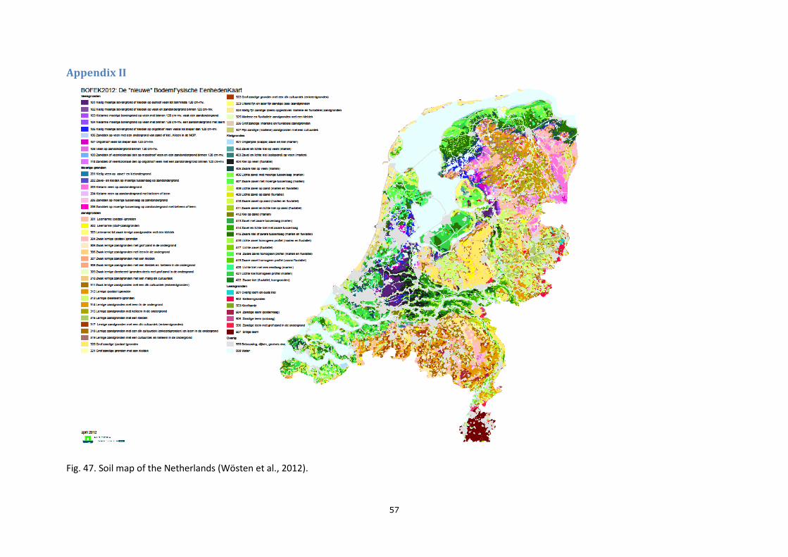
57

Appendix II

Fig. 47. Soil map of the Netherlands (Wösten et al., 2012).

58

Appendix III

Table 4. Soil data used in this thesis study including: type and depth of the soil layers and hydraulic

parameters

Appendix IV

Fig. 48. Fields which was assumed under drought or oxygen stress in year 2013 (red mark) & 2014

(blue mark). Dacom rainfall station (2013 orange circle; 2014 yellow circle) and Eindhoven station

(black circle)

59

Appendix V

Table 5. Soil codes of the fields used for water limited yield simulation

Appendix VI

Fig. 49. SSE of different TSUM2 values ( x axis: TSUM2 y axis: SSE).

60

Appendix VII

Table 6. Hydrological parameters used for fields “fabrie gemeente hoef” and “fabri lutter gemeente”

Abbreviations used here: ORES (residual water content, cm3/cm3), OSAT (saturated water content,

cm3/cm3), ALFA (shape parameter alfa of main drying curve, cm-1), NPAR (shape parameter n), KSAT

(saturated vertical hydraulic conductivity, cm/d), LEXP (exponent in hydraulic conductivity function),

ALFAW (alfa parameter of main wetting curve in case of hysteresis, cm-1), H_ENPR (entry pressure

head, cm).

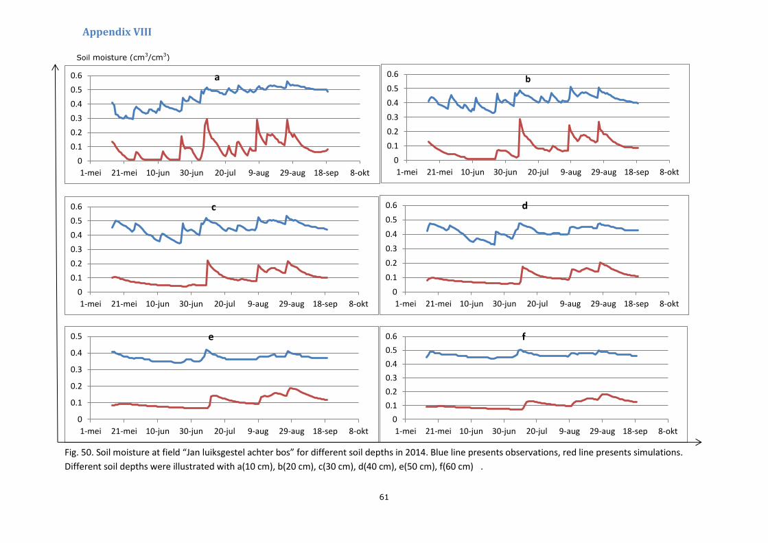
61

Fig. 50. Soil moisture at field “Jan luiksgestel achter bos” for different soil depths in 2014. Blue line presents observations, red line presents simulations.

Different soil depths were illustrated with a(10 cm), b(20 cm), c(30 cm), d(40 cm), e(50 cm), f(60 cm) .

0

0.1

0.2

0.3

0.4

0.5

0.6

1-mei 21-mei 10-jun 30-jun 20-jul 9-aug 29-aug 18-sep 8-okt

a

0

0.1

0.2

0.3

0.4

0.5

0.6

1-mei 21-mei 10-jun 30-jun 20-jul 9-aug 29-aug 18-sep 8-okt

b

0

0.1

0.2

0.3

0.4

0.5

0.6

1-mei 21-mei 10-jun 30-jun 20-jul 9-aug 29-aug 18-sep 8-okt

c

0

0.1

0.2

0.3

0.4

0.5

0.6

1-mei 21-mei 10-jun 30-jun 20-jul 9-aug 29-aug 18-sep 8-okt

d

0

0.1

0.2

0.3

0.4

0.5

1-mei 21-mei 10-jun 30-jun 20-jul 9-aug 29-aug 18-sep 8-okt

e

0

0.1

0.2

0.3

0.4

0.5

0.6

1-mei 21-mei 10-jun 30-jun 20-jul 9-aug 29-aug 18-sep 8-okt

f

Soil moisture (cm3/cm3)

Appendix VIII