Application of the Elliptical Trigonometry Version 2 · A survey on the application of the Elliptical Trigonometry in ... the mathematical topics of Fourier series and ... Fig. 4:

A survey on the application of the Elliptical Trigonometry in industrial electronic systems using controlled waveforms with modeling and

simulating of two functions Elliptic Mar and Elliptic Jes-x

CLAUDE BAYEH Faculty of Engineering II

Lebanese University LEBANON

Email: [email protected] Abstract: - In industrial electronic systems, power converters with power components are used. Each controlled component has its own control circuit. In this paper, the author proposes an original control circuit for each function in order to replace the different existing circuits. The proposed circuit is the representation of an elliptical trigonometric function as “Elliptic Mar” and “Elliptic Jes-x” that are particular cases of the elliptical trigonometry. Thus, with one function, by varying the values of its parameters, the output waveform will change and can describe more than 12 different waveforms. Finally for each function, a block diagram, a model of the circuit and a programming part are treated using Matlab/Simulink. The results of the studied circuit are presented and discussed. Key-words: - Power electronics, power converters, mathematics, trigonometry, multi form signal. 1 Introduction In motor drives, robotics, or other industrial electronic applications, the use of power converters is essential to improve the control and, therefore, the efficiency of the studied system [17],[18]. Power converters and power electronics circuits are generally composed of power components with different characteristics [17]. These components are divided in two categories: the controlled components and the uncontrolled components [17], [19],[20]. The controlled components that are based on semi-conductors like thyristors, Triac and transistors need controlled signals with specified waveforms in order to be applied on their controlled terminals (base or gate) [17],[19]. Thus, each component has its own control source. This paper underlines the importance of the elliptical trigonometric functions in generating different waveforms by varying some parameters of a single function. In a particular case, the Elliptic Mar and the Elliptic Jes-x functions are chosen to be treated. In fact, the elliptical trigonometry is an original study introduced with new concepts [1],[2]. The existed trigonometry (Circular trigonometry) is a particular case of the elliptical trigonometry [6],[7]. The traditional trigonometry has an enormous variety of applications in all scientific domains [6],[7],[8],[9]. It can be considered as the basis and

foundation of many domains as electronics, signal theory, astronomy, navigation, propagation of signals and many others… [10],[11],[12],[13]. Particularly, the mathematical topics of Fourier series and Fourier transforms rely heavily on knowledge of trigonometric functions [10],[11] and find application in a number of areas, including statistics [12],[13]. In this paper, the new concept of the elliptical trigonometry is introduced and few examples are shown and discussed briefly. Figures and results are drawn and simulated using Matlab/Simulink and AutoCAD. A survey on the applications of this trigonometry in the power electronics domains presented in section 2. In the third section, the angular functions are defined, these functions have enormous applications in all domains, and it can be considered as the basis of this trigonometry [1],[2]. The definition of the Elliptical trigonometry is presented and discussed briefly in section 4. In the fifth section, a survey on the Elliptical Trigonometric functions is discussed and two principal functions are presented. In the sections 6 and 7, two functions are studied and discussed briefly with simulation on Simulink/Matlab, their block diagrams are presented, their programming parts and so their modeling circuits. Finally, a conclusion about the elliptical trigonometry is presented in the section 8.

WSEAS TRANSACTIONS on SYSTEMS and CONTROL Claude Bayeh

ISSN: 1991-8763 859 Issue 11, Volume 5, November 2010

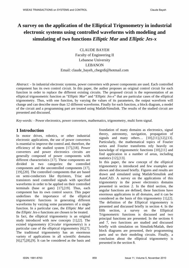
2 A survey on the application of the elliptical trigonometry in engineering domain The used controlled circuits for power transistors (MOSFET, IGBT, etc) differ from those used for Thyristors (GTO, Triac, etc). Designing and modeling circuits for all these controlled components taking into account their different characteristics, take time, and realizing them practically, take time and money. In this paper, for each elliptical trigonometric function, one electronic circuit is proposed to be used in simulation (Labview, Matlab, Simulink etc). For a particular case, in order to control the different existed power components for the function Elliptic Mar (figure 1), two parameters ′푏′ and ′푖′ are used as variable inputs. The output will be the studied elliptical trigonometry function. Thus, the main goal of the Elliptical Trigonometry is to produce a huge number of multi form signals using a single function and by varying some parameters of this function. For a particular case, more than 12 different output signals can be obtained by varying two parameters of the Elliptic Mar function.

Fig. 1: Electronic circuit of the function 퐸푚푎푟 , (푥)

with its inputs and output. 3 The angular functions In order to make a review on the elliptical trigonometry, it is necessary to introduce the definition of the angular functions. In fact, angular functions are new mathematical functions that produce a rectangular signal, in which period is function of angles. Similar to trigonometric functions, the angular functions have the same properties as the precedent, but the difference is that a rectangular signal is obtained instead of a sinusoidal signal [14],[15],[16] and moreover, one can change the width of each positive and negative alternate in the same period. This is not the case of any other trigonometric function. In other hand, one can change the frequency, the amplitude and the width of any period of the signal by using the general form of the angular function.

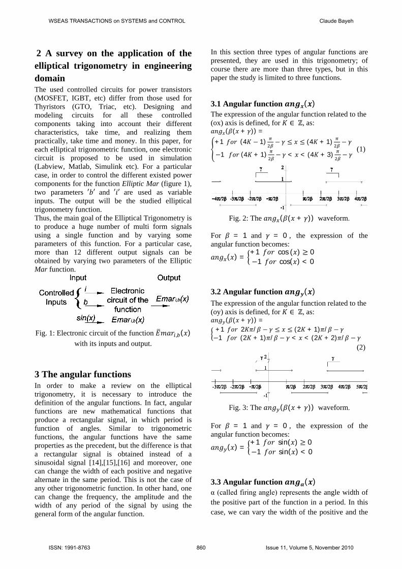
In this section three types of angular functions are presented, they are used in this trigonometry; of course there are more than three types, but in this paper the study is limited to three functions. 3.1 Angular function 풂풏품풙(풙) The expression of the angular function related to the (ox) axis is defined, for 퐾 ∈ ℤ, as: 푎푛푔 (훽(푥 + 훾)) =

+1 푓표푟 (4퐾 − 1) − 훾 ≤ 푥 ≤ (4퐾 + 1) − 훾

−1 푓표푟 (4퐾 + 1) − 훾 < 푥 < (4퐾 + 3) − 훾 (1)

Fig. 2: The 푎푛푔 (훽(푥 + 훾)) waveform.

For 훽 = 1 and 훾 = 0 , the expression of the angular function becomes:

푎푛푔 (푥) =+1 푓표푟 cos (푥) ≥ 0 −1 푓표푟 cos(푥) < 0

3.2 Angular function 풂풏품풚(풙) The expression of the angular function related to the (oy) axis is defined, for 퐾 ∈ ℤ, as: 푎푛푔 (훽(푥 + 훾)) =

+1 푓표푟 2퐾휋/훽 − 훾 ≤ 푥 ≤ (2퐾 + 1)휋/훽 − 훾 −1 푓표푟 (2퐾 + 1)휋/훽 − 훾 < 푥 < (2퐾 + 2)휋/훽 − 훾

(2)


For 훽 = 1 and 훾 = 0 , the expression of the angular function becomes:

푎푛푔 (푥) =+1 푓표푟 sin(푥) ≥ 0 −1 푓표푟 sin(푥) < 0

3.3 Angular function 풂풏품휶(풙) α (called firing angle) represents the angle width of the positive part of the function in a period. In this case, we can vary the width of the positive and the



negative part by varying only α. The firing angle must be positive. 푎푛푔 훽(푥 + 훾) =

⎩⎪⎨

⎪⎧

+1 푓표푟 (2퐾휋 − 훼)/훽 − 훾 ≤ 푥 ≤ (2퐾휋 + 훼)/훽 − 훾

−1 푓표푟 (2퐾휋 + 훼)/훽 − 훾 < 푥 < (2(퐾 + 1)휋 − 훼)/훽 − 훾

(3)


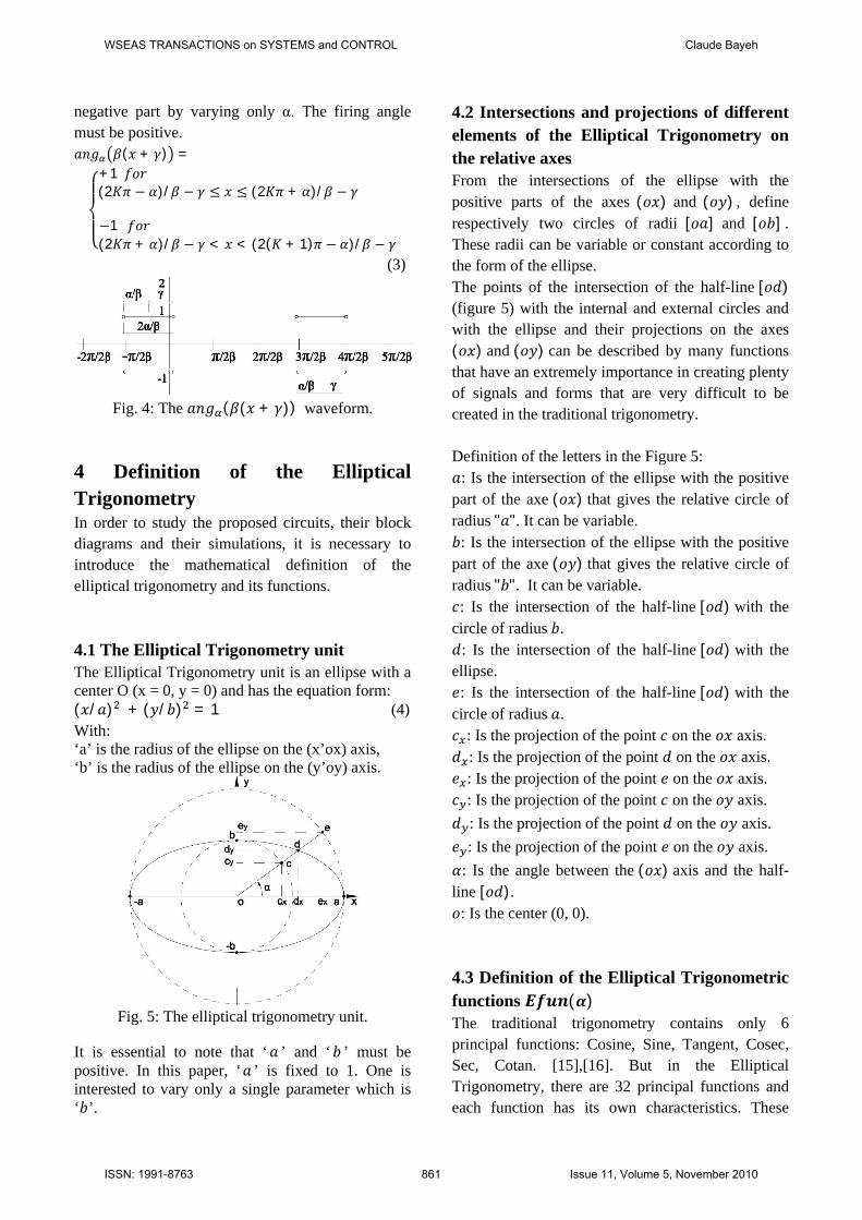
4 Definition of the Elliptical Trigonometry In order to study the proposed circuits, their block diagrams and their simulations, it is necessary to introduce the mathematical definition of the elliptical trigonometry and its functions. 4.1 The Elliptical Trigonometry unit The Elliptical Trigonometry unit is an ellipse with a center O (x = 0, y = 0) and has the equation form: (푥/푎) + (푦/푏) = 1 (4) With: ‘a’ is the radius of the ellipse on the (x’ox) axis, ‘b’ is the radius of the ellipse on the (y’oy) axis.

Fig. 5: The elliptical trigonometry unit.

It is essential to note that ‘푎 ’ and ‘푏 ’ must be positive. In this paper, ‘푎 ’ is fixed to 1. One is interested to vary only a single parameter which is ‘푏’.

4.2 Intersections and projections of different elements of the Elliptical Trigonometry on the relative axes From the intersections of the ellipse with the positive parts of the axes (표푥) and (표푦) , define respectively two circles of radii [표푎] and [표푏] . These radii can be variable or constant according to the form of the ellipse. The points of the intersection of the half-line [표푑) (figure 5) with the internal and external circles and with the ellipse and their projections on the axes (표푥) and (표푦) can be described by many functions that have an extremely importance in creating plenty of signals and forms that are very difficult to be created in the traditional trigonometry. Definition of the letters in the Figure 5: 푎: Is the intersection of the ellipse with the positive part of the axe (표푥) that gives the relative circle of radius "푎". It can be variable. 푏: Is the intersection of the ellipse with the positive part of the axe (표푦) that gives the relative circle of radius "푏". It can be variable. 푐: Is the intersection of the half-line [표푑) with the circle of radius 푏. 푑: Is the intersection of the half-line [표푑) with the ellipse. 푒: Is the intersection of the half-line [표푑) with the circle of radius 푎. 푐 : Is the projection of the point 푐 on the 표푥 axis. 푑 : Is the projection of the point 푑 on the 표푥 axis. 푒 : Is the projection of the point 푒 on the 표푥 axis. 푐 : Is the projection of the point 푐 on the 표푦 axis. 푑 : Is the projection of the point 푑 on the 표푦 axis. 푒 : Is the projection of the point 푒 on the 표푦 axis. 훼: Is the angle between the (표푥) axis and the half-line [표푑). 표: Is the center (0, 0). 4.3 Definition of the Elliptical Trigonometric functions 푬풇풖풏(휶) The traditional trigonometry contains only 6 principal functions: Cosine, Sine, Tangent, Cosec, Sec, Cotan. [15],[16]. But in the Elliptical Trigonometry, there are 32 principal functions and each function has its own characteristics. These



functions give a new vision of the world and will be used in all scientific domains and make a new challenge in the reconstruction of the science especially when working on the economical side of the power of electrical circuits, the electrical transmission, the signal theory and many other domains [15],[17]. The functions 퐶푗푒푠(훼),퐶푚푎푟(훼),퐶푡푒푟(훼) and 퐶푗푒푠 (훼) , which are respectively equivalent to cosine, sine, tangent and cotangent. These functions are particular cases of the “Circular Trigonometry”. The names of the cosine, sine, tangent and cotangent are replaced respectively by Circular Jes, Circular Mar, Circular Ter and Circular Jes-y. 퐶푗푒푠(훼) ⇔ 푐표푠(훼); 퐶푚푎푟(훼) ⇔ 푠푖푛(훼) 퐶푡푒푟(훼) ⇔ 푡푎푛(훼); 퐶푗푒푠 (훼) ⇔ 푐표푡푎푛(훼). The Elliptical Trigonometric functions are denoted using the following abbreviation “퐸푓푢푛(훼)”: -the first letter “E” is related to the Elliptical trigonometry. -the word “푓푢푛(훼)” represents the specific function name that is defined hereafter: (refer to Figure 5). • Elliptical Jes functions: El. Jes: 퐸푗푒푠(훼) = = (5)

El. Jes-x: 퐸푗푒푠 (훼) = = ( )( ) (6)

El. Jes-y: 퐸푗푒푠 (훼) = = ( )( ) (7)

• Elliptical Mar functions:

El. Mar: 퐸푚푎푟(훼) = = (8)

El. Mar-x: 퐸푚푎푟 (훼) = = ( )( ) (9)

El. Mar-y: 퐸푚푎푟 (훼) = = ( )( ) (10)

• Elliptical Ter functions: El. Ter: 퐸푡푒푟(훼) = ( )

( ) (11)

El. Ter-x:

퐸푡푒푟 (훼) = ( )( ) = 퐸푡푒푟(훼) ∙ 퐶푡푒푟(훼) (12)

El. Ter-y: 퐸푡푒푟 (훼) =( )

( ) = ( )( ) (13)

• Elliptical Rit functions: El. Rit: 퐸푟푖푡(훼) = = = ( )

( ) (14)

El. Rit-y: 퐸푟푖푡 (훼) = = ( )( ) (15)

• Elliptical Raf functions:

El. Raf: 퐸푟푎푓(훼) = = 퐶푡푒푟(훼).퐸푗푒푠(훼) (16)

El. Raf-x: 퐸푟푎푓 (훼) = = ( )( ) (17)

• Elliptical Ber functions: El. Ber: 퐸푏푒푟(훼) = ( )

( ) (18)

El. Ber-x:

퐸푏푒푟 (훼) = ( )( ) = 퐸푏푒푟(훼) ∙ 퐶푡푒푟(훼) (19)

El. Ber-y: 퐸푏푒푟 (훼) =( )( ) = ( )

( ) (20)

4.4 The reciprocal of the Elliptical Trigonometric function 퐸푓푢푛 (훼) is defined as the inverse function of

퐸푓푢푛(훼) . (퐸푓푢푛−1(훼) = 1/퐸푓푢푛(훼)) . In this way the reduced number of functions is equal to 32 principal functions.

E.g.: 퐸푗푒푠 (훼) = 1(훼)

4.5 Definition of the Absolute Elliptical Trigonometric functions 푬풇풖풏(휶) The Absolute Elliptical Trigonometry is introduced to create the absolute value of a function by varying only one parameter without using the absolute value “| |”. The advantage is that one can change and control the sign of an Elliptical Trigonometric function without using the absolute value in an expression. Some functions are treated to get an idea about the importance of this new definition. To obtain the Absolute Elliptical Trigonometry for a specified function (e.g.: 퐸푗푒푠(훼) ) we must multiply it by the corresponding Angular Function (e.g.:

푎푛푔 (훼) with 푖 ∈ ℕ ) in a way to obtain the original function if 푖 is even, and to obtain the absolute value of the function if 푖 is odd (e.g.: |퐸푗푒푠(훼)|). If the function doesn’t have a negative part (not alternative) it will be multiplied by 푎푛푔 (훽(훼 −

훾)) to obtain an alternating signal which form depends on the value of the frequency “훽” and the translation value “ 훾 ”. By varying the last parameters, one can get a multi form signals.



• 퐸푗푒푠 (훼) = 푎푛푔 (훼) ∙ 퐸푗푒푠(훼) (21)

=푎푛푔 (훼) ∙ 퐸푗푒푠(훼) = |퐸푗푒푠(훼)| 푖푓 푖 = 1

푎푛푔 (훼) ∙ 퐸푗푒푠(훼) = 퐸푗푒푠(훼) 푖푓 푖 = 2

• 퐸푗푒푠 , (훼) = 푎푛푔 (훼 − 훾) ∙ 퐸푗푒푠 (훼) (22)

= 푎푛푔 (훼 − 훾) ∙ 퐸푗푒푠 (훼) 푖푓 푖 = 1퐸푗푒푠 (훼) 푖푓 푖 = 2

• 퐸푗푒푠 , (훼) = 푎푛푔 (2훼) ∙ 퐸푗푒푠 (훼) (23)

=푎푛푔 (2훼) ∙ 퐸푗푒푠 (훼) = |퐸푗푒푠 (훼)| 푖푓 푖 = 1퐸푗푒푠 (훼) 푖푓 푖 = 2

• 퐸푚푎푟 (훼) = 푎푛푔 (훼) ∙ 퐸푚푎푟(훼) (24)

• 퐸푚푎푟 , (훼) = 푎푛푔 (2훼) ∙ 퐸푚푎푟 (훼) (25)

• 퐸푚푎푟 , (훼) = 푎푛푔 (훼 − 훾) ∙ 퐸푚푎푟 (훼) (26)

• 퐸푟푖푡 (훼) = 푎푛푔 (훼) ∙ 퐸푟푖푡(훼) (27) And so on… 5 A survey on the Elliptical Trigonometric functions As previous sections, a brief study on the Elliptical Trigonometry is given. Two functions of 32 are treated; the others functions can be easily interpreted using formulae from (5) to (20). Elliptic cosine and Elliptic sine that appear in the previous articles [1] and [2], are particular cases of the Elliptic Jes and Elliptic Mar respectively. For this study the following conditions are taken: - 푎 = 1 - 푏 > 0 the radius of the ellipse on the 푦′표푦 axis. - 푖 ∈ ℕ 5.1 Determination of the Elliptic Jes function The Elliptical form in the figure 5 is written as the equation (4). Thus, given (5), the Elliptic Jes function can be determined using the following method. In fact: 퐶푡푒푟(훼) = = , it is significant to replace the

equation 푦 = 퐶푡푒푟(훼). 푥 in that defined in (4).

+ 퐶푡푒푟(훼) = 1 + 퐶푡푒푟(훼) = 1 ⇒

퐸푗푒푠 (훼) = ±

( )

Therefore: •퐸푗푒푠 (훼) =

( ) for − ≤ 푥 ≤ ; ≥ 0

•퐸푗푒푠 (훼) = ( )

for < 푥 < ; < 0

Thus, the expression of the Elliptic Jes can be unified by using the angular function expression (1), therefore the expression becomes: 퐸푗푒푠 (훼) = ( )

( )⇒

퐸푗푒푠 (푥) = ( )

( ) (28)

• Expression of the Absolute Elliptic Jes:

퐸푗푒푠 , (푥) = ( )

( )∙ 푎푛푔 (푥) (29)

The Absolute Elliptic Jes is a powerful function that can produce more than 12 different signals by varying only two parameters 푖 and 푏. Similar to the cosine function in the traditional trigonometry, the Absolute Elliptic Jes is more general than the precedent. 5.2 Determination of the Elliptic Mar function The elliptical form in the figure 5 is written as the equation (4). Thus, given (8), the Elliptic Mar function can be determined using the following method. In fact: 퐶푡푒푟(훼) = = ⇒ 푥 = ( ) , it is significant

to replace the equation 푥 = ( ) in that defined in

(4). Thus, (∙ ( )) + (푦/푏) = 1 ⇒

퐸푚푎푟 (훼) = =± ( )

( )

⇒ 퐸푚푎푟푏(푥) = 푦푏 =

±푎푏Cter (푥)

1+ 푎푏Cter (푥)

2

Therefore:

• 퐸푚푎푟 (푥) = ( )

( ) for 0 ≤ 푥 <



• 퐸푚푎푟 (푥) = ( )

( ) for < 푥 ≤ 휋

• 퐸푚푎푟 (푥) = ( )

( ) for 휋 ≤ 푥 < 3

• 퐸푚푎푟 (푥) = ( )

( ) for 3 ≤ 푥 ≤ 2휋

Thus, the expression of the elliptic Mar can be unified by using the angular function expression (1), therefore the expression becomes: 퐸푚푎푟 (푥) = ( ) ( )

( ) (30)

• Expression of the Absolute Elliptic Mar:

퐸푚푎푟 , (푥) = 퐸푚푎푟 (푥) ∙ 푎푛푔 (푥) (31)

The Absolute Elliptic Mar is a powerful function that can produce more than 12 different signals by varying only two parameters 푖 and 푏. Similar to the sine function in the traditional trigonometry, the Absolute Elliptic Mar is more general than the precedent. 5.3 Original formulae of the Elliptical Trigonometry In this sub-section, a brief review on some remarkable formulae formed using the elliptical trigonometric functions.

• 퐸푗푒푠 (푥) + 퐸푚푎푟 (푥) = 1 (32)

In fact: 퐸푗푒푠 (푥) + 퐸푚푎푟 (푥) =

( )

( )+ ( ) ( )

( )=

( )+ ( )

( ) =

( )

( ) =

( )

( )= 1

• ( ) ( )

+( ) ( )

= 1 (33)

In fact:

퐸푗푒푠 (푥) + 퐸푚푎푟 (푥) = ( )( ) + ( )

( )

=( )

⇒ ( ) ( ) = 퐶푗푒푠(푥)

And

퐸푗푒푠 (푥) + 퐸푚푎푟 (푥) = ( )( ) + ( )

( )

=( )

⇒ 1퐸푗푒푠푦

2(푥)+퐸푚푎푟푦2(푥)= 퐶푚푎푟(푥)

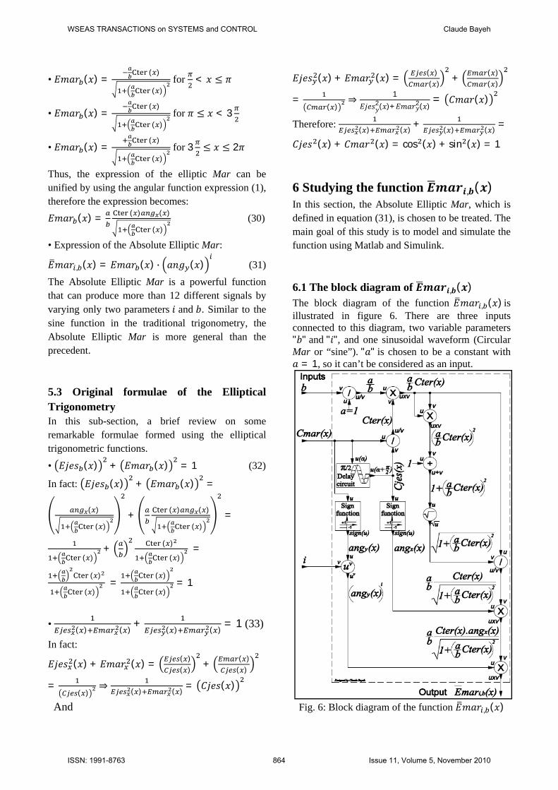
Therefore: ( ) ( ) + ( ) ( ) =

퐶푗푒푠 (푥) + 퐶푚푎푟 (푥) = cos (푥) + sin (푥) = 1 6 Studying the function 푬풎풂풓풊,풃(풙) In this section, the Absolute Elliptic Mar, which is defined in equation (31), is chosen to be treated. The main goal of this study is to model and simulate the function using Matlab and Simulink. 6.1 The block diagram of 푬풎풂풓풊,풃(풙) The block diagram of the function 퐸푚푎푟 , (푥) is illustrated in figure 6. There are three inputs connected to this diagram, two variable parameters "푏" and "푖", and one sinusoidal waveform (Circular Mar or “sine”). "푎" is chosen to be a constant with 푎 = 1, so it can’t be considered as an input.

Fig. 6: Block diagram of the function 퐸푚푎푟 , (푥)



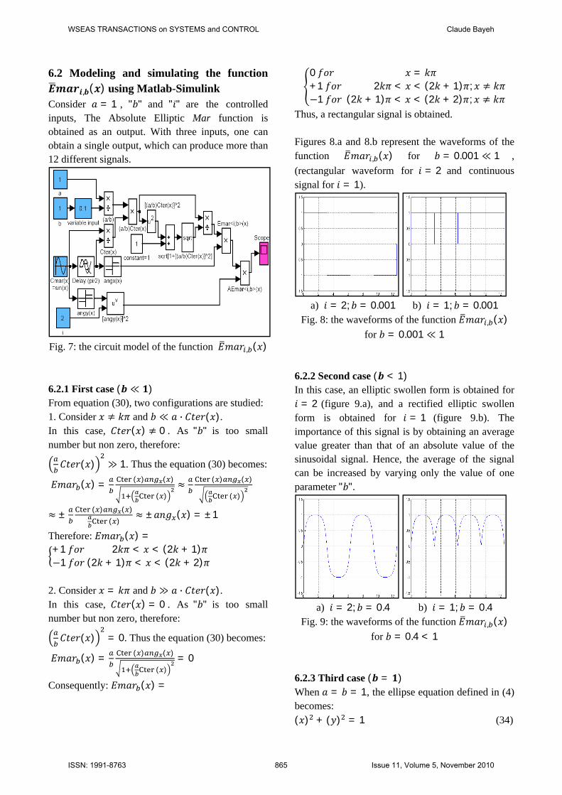
6.2 Modeling and simulating the function 푬풎풂풓풊,풃(풙) using Matlab-Simulink Consider 푎 = 1 , "푏" and "푖" are the controlled inputs, The Absolute Elliptic Mar function is obtained as an output. With three inputs, one can obtain a single output, which can produce more than 12 different signals.

Fig. 7: the circuit model of the function 퐸푚푎푟 , (푥) 6.2.1 First case (풃 ≪ ퟏ) From equation (30), two configurations are studied: 1. Consider 푥 ≠ 푘휋 and 푏 ≪ 푎 ∙ 퐶푡푒푟(푥). In this case, 퐶푡푒푟(푥) ≠ 0 . As "푏" is too small number but non zero, therefore:

퐶푡푒푟(푥) ≫ 1. Thus the equation (30) becomes:

퐸푚푎푟 (푥) = ( ) ( )

( )≈ ( ) ( )

( )

≈ ± ( ) ( ) ( )

≈ ±푎푛푔 (푥) = ±1

Therefore: 퐸푚푎푟 (푥) = +1 푓표푟 2푘휋 < 푥 < (2푘 + 1)휋 −1 푓표푟 (2푘 + 1)휋 < 푥 < (2푘 + 2)휋

2. Consider 푥 = 푘휋 and 푏 ≫ 푎 ∙ 퐶푡푒푟(푥). In this case, 퐶푡푒푟(푥) = 0 . As "푏" is too small number but non zero, therefore:

퐶푡푒푟(푥) = 0. Thus the equation (30) becomes:

퐸푚푎푟 (푥) = ( ) ( )

( )= 0

Consequently: 퐸푚푎푟 (푥) =

0 푓표푟 푥 = 푘휋 +1 푓표푟 2푘휋 < 푥 < (2푘 + 1)휋; 푥 ≠ 푘휋−1 푓표푟 (2푘 + 1)휋 < 푥 < (2푘 + 2)휋; 푥 ≠ 푘휋

Thus, a rectangular signal is obtained. Figures 8.a and 8.b represent the waveforms of the function 퐸푚푎푟 , (푥) for 푏 = 0.001 ≪ 1 , (rectangular waveform for 푖 = 2 and continuous signal for 푖 = 1).

a) 푖 = 2; 푏 = 0.001 b) 푖 = 1; 푏 = 0.001

Fig. 8: the waveforms of the function 퐸푚푎푟 , (푥) for 푏 = 0.001 ≪ 1

6.2.2 Second case (풃 < 1) In this case, an elliptic swollen form is obtained for 푖 = 2 (figure 9.a), and a rectified elliptic swollen form is obtained for 푖 = 1 (figure 9.b). The importance of this signal is by obtaining an average value greater than that of an absolute value of the sinusoidal signal. Hence, the average of the signal can be increased by varying only the value of one parameter "푏".

a) 푖 = 2; 푏 = 0.4 b) 푖 = 1; 푏 = 0.4

Fig. 9: the waveforms of the function 퐸푚푎푟 , (푥) for 푏 = 0.4 < 1

6.2.3 Third case (풃 = ퟏ) When 푎 = 푏 = 1, the ellipse equation defined in (4) becomes: (푥) + (푦) = 1 (34)



This is the equation of a circle of radius 푟 = 1. • The Elliptic Mar function defined in (8) becomes:

퐸푚푎푟(훼) = = = 퐶푚푎푟(훼) = sin(훼) • The Elliptic Jes function defined in (5) becomes: 퐸푗푒푠(훼) = = = 퐶푗푒푠(훼) = cos(훼)

Therefore, 퐸푚푎푟 , (푥) = sin(푥) ∙ 푎푛푔 (푥) (35)

Figures 10.a and 10.b represent the waveforms of the function 퐸푚푎푟 , (푥) for 푏 = 1 , (sinusoidal signal for 푖 = 2 and rectified sinusoidal signal for 푖 = 1).

a) 푖 = 2; 푏 = 1 b) 푖 = 1; 푏 = 1

Fig. 10: the waveforms of the function 퐸푚푎푟 , (푥) for 푏 = 1

6.2.4 Fourth case (풃 > 1) In this case, an elliptic deflated form is obtained for 푖 = 2 (figure 11.a), and a rectified elliptic deflated form is obtained for 푖 = 1 (figure 11.b). The importance of this signal is by obtaining an average value smaller than that of an absolute value of the sinusoidal signal. Hence, the average of the signal can be decreased by varying only the value of one parameter "푏".

a) 푖 = 2; 푏 = 6 b) 푖 = 1; 푏 = 6

Fig. 11: the waveforms of the function 퐸푚푎푟 , (푥) for 푏 = 6 > 1

6.2.5 Fifth case (풃 ≫ ퟏ) From equation (30), two configurations are studied: 1. Consider 푥 ≠ ( )휋 and 푏 ≫ 푎 ∙ 퐶푡푒푟(푥). In this case, 퐶푡푒푟(푥) ≠ ±∞ . As "푏" is too large number but non infinite, therefore:

퐶푡푒푟(푥) = 휀 ≪ 1. It is much smaller than the

unit. Thus the equation (30) becomes:

퐸푚푎푟 (푥) = ( ) ( )

( )≈ √ ∙ ( )

√, by

using Taylor development for the first degree

퐸푚푎푟 (푥) = √휀 ∙ 푎푛푔 (푥) 1 − ≈ √휀 ∙ 푎푛푔 (푥)

Therefore:

퐸푚푎푟 (푥) = 0 푓표푟 2푘휋 < 푥 < (2푘 + 1)휋 0 푓표푟 (2푘 + 1)휋 < 푥 < (2푘 + 2)휋

2. Consider 푥 = ( )휋 and 푏 ≪ 푎 ∙ 퐶푡푒푟(푥). In this case, 퐶푡푒푟(푥) = ±∞ . As "푏" is too large number but non infinite, therefore:

퐶푡푒푟(푥) ≫ 1. Thus the equation (30) becomes:

퐸푚푎푟 (푥) = ( ) ( )

( )≈ ( ) ( )

( )

≈ ± ( ) ( ) ( )

≈ ±푎푛푔 (푥) = ±1

Consequently: 퐸푚푎푟 (푥) =

⎩⎪⎪⎨

⎪⎪⎧0 푓표푟 2푘휋 < 푥 < (2푘 + 1)휋; 푥 ≠ ( )

0 푓표푟 (2푘 + 1)휋 < 푥 < (2푘 + 2)휋; 푥 ≠ ( )

+1 푓표푟 2푘휋 < 푥 < (2푘 + 1)휋; 푥 = ( )

−1 푓표푟 (2푘 + 1)휋 < 푥 < (2푘 + 2)휋; 푥 = ( )

Thus, an impulse signal is obtained. Figures 12.a and 12.b represent the waveforms of the function 퐸푚푎푟 , (푥) for 푏 = 100 ≫ 1, (impulse train with positive and negative part for 푖 = 2 and impulse train with positive part only for 푖 = 1).

a) 푖 = 2; 푏 = 100 b) 푖 = 1; 푏 = 100

Fig. 12: the waveforms of the function 퐸푚푎푟 , (푥) for 푏 = 100 ≫ 1



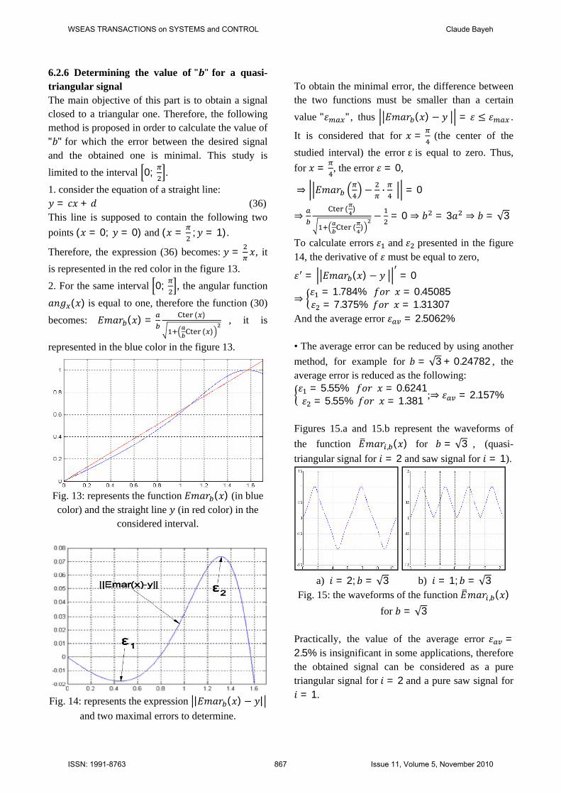
6.2.6 Determining the value of "풃" for a quasi-triangular signal The main objective of this part is to obtain a signal closed to a triangular one. Therefore, the following method is proposed in order to calculate the value of "푏" for which the error between the desired signal and the obtained one is minimal. This study is limited to the interval 0; .

1. consider the equation of a straight line: 푦 = 푐푥 + 푑 (36) This line is supposed to contain the following two points (푥 = 0; 푦 = 0) and (푥 = ;푦 = 1).

Therefore, the expression (36) becomes: 푦 = 푥, it is represented in the red color in the figure 13. 2. For the same interval 0; , the angular function

푎푛푔 (푥) is equal to one, therefore the function (30)

becomes: 퐸푚푎푟 (푥) = ( )

( ), it is

represented in the blue color in the figure 13.

Fig. 13: represents the function 퐸푚푎푟 (푥) (in blue color) and the straight line 푦 (in red color) in the

considered interval.

Fig. 14: represents the expression |퐸푚푎푟 (푥) − 푦|

and two maximal errors to determine.

To obtain the minimal error, the difference between the two functions must be smaller than a certain value "휀 ", thus 퐸푚푎푟 (푥) − 푦 = 휀 ≤ 휀 .

It is considered that for 푥 = (the center of the studied interval) the error ε is equal to zero. Thus, for 푥 = , the error 휀 = 0,

⇒ 퐸푚푎푟 − ∙ = 0

⇒ ( )

( )− = 0 ⇒ 푏 = 3푎 ⇒ 푏 = √3

To calculate errors 휀 and 휀 presented in the figure 14, the derivative of 휀 must be equal to zero,

휀 = 퐸푚푎푟 (푥) − 푦 = 0

⇒ 휀 = 1.784% 푓표푟 푥 = 0.45085휀 = 7.375% 푓표푟 푥 = 1.31307

And the average error 휀 = 2.5062% • The average error can be reduced by using another method, for example for 푏 = √3 + 0.24782 , the average error is reduced as the following: 휀 = 5.55% 푓표푟 푥 = 0.6241휀 = 5.55% 푓표푟 푥 = 1.381 ;⇒ 휀 = 2.157%

Figures 15.a and 15.b represent the waveforms of the function 퐸푚푎푟 , (푥) for 푏 = √3 , (quasi-triangular signal for 푖 = 2 and saw signal for 푖 = 1).

a) 푖 = 2; 푏 = √3 b) 푖 = 1; 푏 = √3

Fig. 15: the waveforms of the function 퐸푚푎푟 , (푥) for 푏 = √3

Practically, the value of the average error 휀 =2.5% is insignificant in some applications, therefore the obtained signal can be considered as a pure triangular signal for 푖 = 2 and a pure saw signal for 푖 = 1.



Tables 1 and 2 represent a summary of different waveforms obtained using the Elliptic functions 퐸푚푎푟 , (푥) and 퐸푗푒푠 , (푥).

풃

Absolute Elliptic Mar " 푬풎풂풓풊,풃(풙)" 풊 = ퟐ 풊 = ퟏ

b<<1 Rectangle signal Continuous signal b<1 Elliptical swollen

signal Rectified elliptical

swollen signal b=1 Sinusoidal signal (sine

wave form) Rectified sinusoidal

signal b=√3 Quasi-triangluar signal Saw signal b>1 Elliptical deflated


deflated signal b>>1 Impulse train with

positive and negative pulses

Impulse train with positive part only

Table 1: summary of multi form signals obtained using the Absolute Elliptic Mar function.

풃

Absolute Elliptic Jes " 푬풋풆풔풊,풃(풙)" 풊 = ퟐ 풊 = ퟏ

b<<1 Impulse train with positive part only

Impulse train with positive and

negative pulses b<1 Elliptical deflated


deflated signal b=√3/3 Quasi-triangluar

signal Saw signal

b=1 Sinusoidal signal (cosine wave form)

Rectified sinusoidal signal

b>1 Elliptical swollen signal

Rectified elliptical swollen signal

b>>1 Rectangle signal Continuous signal Table 2: summary of multi form signals obtained

using the Absolute Elliptic Jes function. These types of signals are widely used in power electronics, electrical generators and in transmission of analog signals [17]. 6.3 First conclusion As presented previously, the Elliptic Mar function takes different waveforms by varying the parameter "푏" . The same analysis can be treated using the parameter "푎". Therefore, the same waveforms can be obtained. Practically, instead of varying the value of "푏" from 0 to +∞ in a goal to obtain all waveforms, by introducing "푎", one can change the values of "푏" or "푎" form 0 to 1 in a way to obtain the desired waveform. E.g.: = = .

6.4 programming the Elliptic Mar function in Matlab As presented and analyzed in the previous section, the Elliptic Mar function can be also programmed and written in the Matlab software. Thus, the elliptical trigonometry functions can be used in any industrial applications. The following program represents the detailed steps in writing the Elliptic Mar function in Matlab. %------------------------------------------------------------------- %Programming the Elliptic Mar function in Matlab %Introduced by Claude Ziad Bayeh a=1; x=-15:0.0001:15; clc fprintf('Absolute Elliptic Mar “AEmar”\n'); repeat='y'; while repeat=='y' b=input('determine the form of the Elliptic

trigonometry: b='); fprintf('b is a variable can be changed to obtain

different signals \n'); %b is the intersection of the Ellipse and the axe y'oy in the positive part.

if b<0, b error('ATTENTION: ERROR b must be greater than

Zero'); end; fprintf('AEmar=Emar*(angy(x))î\n'); i=input('for Absolute Elliptic Mar put 1, for Elliptic

Mary put 2: i='); if i<0, i error('ATTENTION: ERROR i must be greater or

equal to Zero'); end; Ejes=(1./(sqrt(1.+((a/b).*tan(x)).^2))).*angx(x);

Emar=(1./(sqrt(1.+((a/b).*tan(x)).^2))).*angx(x).*tan(x).*a/b; % the Elliptic Mar "Emar"

AEmar=Emar.*(angy(x)).î; % Absolute Elliptic Mar plot(x,AEmar); axis([0 4*pi -1.5 1.5]); grid on; fprintf('Do you want to repeat ?\nPress y for ''Yes'' or

any key for ''No''\n'); repeat=input('Y/N=','s'); %string input clc; close all end; %End while %------------------------------------------------------------------- 7 Studying the function 푬풋풆풔풙풃풊 (풙) In this section, a brief study on the Absolute Elliptic Jes-x. The main goal of this study is to model and simulate the function using Matlab and Simulink.



7.1 The Elliptic Jes-x function The elliptical form in the figure 5 is written as the equation (4). Thus, given (6), the Elliptical Jes-x function can be determined. In fact:

퐸푗푒푠 (푥) = ( )( ) = ( )

( )∙ ( ) (37)

• Expression of the Absolute Elliptic Jes-x

퐸푗푒푠 (푥) = 퐸푗푒푠 (푥) ∙ 푎푛푔 (푥 − 훾) (38)

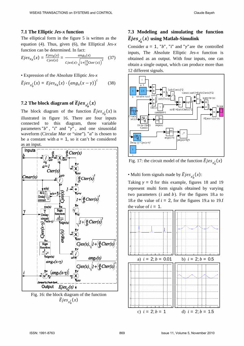
7.2 The block diagram of 푬풋풆풔풙풃풊 (풙) The block diagram of the function 퐸푗푒푠 (푥) is illustrated in figure 16. There are four inputs connected to this diagram, three variable parameters "푏" , "푖" and "훾" , and one sinusoidal waveform (Circular Mar or “sine”). "푎" is chosen to be a constant with 푎 = 1, so it can’t be considered as an input.

Fig. 16: the block diagram of the function 퐸푗푒푠 (푥)

7.3 Modeling and simulating the function 푬풋풆풔풙풃풊 (풙) using Matlab-Simulink Consider 푎 = 1 , "푏" , "푖" and "훾"are the controlled inputs, The Absolute Elliptic Jes-x function is obtained as an output. With four inputs, one can obtain a single output, which can produce more than 12 different signals.

Fig. 17: the circuit model of the function 퐸푗푒푠 (푥)

• Multi form signals made by 퐸푗푒푠 (푥):

Taking 훾 = 0 for this example, figures 18 and 19 represent multi form signals obtained by varying two parameters (푖 and 푏). For the figures 18.a to 18.e the value of 푖 = 2, for the figures 19.a to 19.f the value of 푖 = 1.

a) 푖 = 2; 푏 = 0.01 b) 푖 = 2; 푏 = 0.5

c) 푖 = 2; 푏 = 1 d) 푖 = 2; 푏 = 1.5



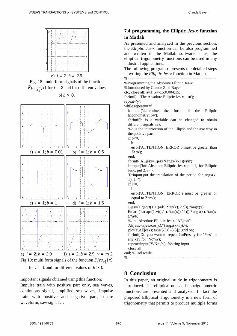
e) 푖 = 2; 푏 = 2.9

Fig. 18: multi form signals of the function 퐸푗푒푠 (푥) for 푖 = 2 and for different values

of 푏 > 0.

a) 푖 = 1; 푏 = 0.01 b) 푖 = 1; 푏 = 0.5

c) 푖 = 1; 푏 = 1 d) 푖 = 1; 푏 = 1.5

e) 푖 = 2; 푏 = 2.9 f) 푖 = 2; 푏 = 2.9; 훾 = 휋/2 Fig.19: multi form signals of the function 퐸푗푒푠 (푥)

for 푖 = 1 and for different values of 푏 > 0. Important signals obtained using this function: Impulse train with positive part only, sea waves, continuous signal, amplified sea waves, impulse train with positive and negative part, square waveform, saw signal …

7.4 programming the Elliptic Jes-x function in Matlab As presented and analyzed in the previous section, the Elliptic Jes-x function can be also programmed and written in the Matlab software. Thus, the elliptical trigonometry functions can be used in any industrial applications. The following program represents the detailed steps in writing the Elliptic Jes-x function in Matlab. %------------------------------------------------------------------- %Programming the Absolute Elliptic Jes-x %Introduced by Claude Ziad Bayeh clc; close all; a=1; x=-15:0.004:15; fprintf('---The Absolute Elliptic Jes-x---\n'); repeat='y'; while repeat=='y' b=input('determine the form of the Elliptic

trigonometry: b='); fprintf('b is a variable can be changed to obtain

different signals \n'); %b is the intersection of the Ellipse and the axe y'oy in

the positive part. if b<0, b error('ATTENTION: ERROR b must be greater than

Zero'); end; fprintf('AEjesx=Ejesx*(angx(x-T))î\n'); i=input('for Absolute Elliptic Jes-x put 1, for Elliptic

Jes-x put 2: i='); T=input('put the translation of the period for angx(x-

T), T='); if i<0, i error('ATTENTION: ERROR i must be greater or

equal to Zero'); end; Ejes=(1./(sqrt(1.+((a/b).*tan(x)).^2))).*angx(x);

Emar=(1./(sqrt(1.+((a/b).*tan(x)).^2))).*angx(x).*tan(x).*a/b;

% the Absolute Elliptic Jes-x "AEjesx" AEjesx=Ejes./cos(x).*(angx(x-T)).î; plot(x,AEjesx); axis([-2 8 -3 3]); grid on; fprintf('Do you want to repeat ?\nPress y for ''Yes'' or

any key for ''No''\n'); repeat=input('Y/N=','s'); %string input close all end; %End while %------------------------------------------------------------------- 8 Conclusion In this paper, an original study in trigonometry is introduced. The elliptical unit and its trigonometric functions are presented and analyzed. In fact the proposed Elliptical Trigonometry is a new form of trigonometry that permits to produce multiple forms



of signals by varying some parameters; it can be used in numerous scientific domains and particularly in mathematics and in engineering. For the case treated in this paper, 32 elliptical trigonometric functions are defined; only two functions are analyzed and simulated using software as Matlab-Simulink. In general, a connection cable with specific transmission data protocol connects any industrial system to the computer. One can use the studied functions in order to generate control signals in need for power components of the industrial system. The elliptical trigonometry functions will be widely used in electronic domain especially in power electronics. Thus, several studied will be improved and developed after introducing the new functions of the elliptic trigonometry. Some mathematical expressions and electronic circuits will be replaced by simplified expressions and reduced circuits. References: [1] Claude Bayeh, M. Bernard, N. Moubayed,

Introduction to the elliptical trigonometry, WSEAS Transactions on Mathematics, Issue 9, Volume 8, September 2009, pp. 551-560.

[2] N. Moubayed, Claude Bayeh, M. Bernard, A survey on modeling and simulation of a signal source with controlled waveforms for industrial electronic applications, WSEAS Transactions on Circuits and Systems, Issue 11, Volume 8, November 2009, pp. 843-852.

[3] M. Christopher, From Eudoxus to Einstein: A History of Mathematical Astronomy, Cambridge University Press, 2004.

[4] Eric W. Weisstein, Trigonometric Addition Formulas, Wolfram MathWorld, 1999-2009.

[5] Paul A. Foerster, Algebra and Trigonometry: Functions and Applications, Addison-Wesley publishing company, 1998.

[6] Robert C.Fisher and Allen D.Ziebur, Integrated Algebra and Trigonometry with Analytic Geometry, Pearson Education Canada, 2006.

[7] E. Demiralp, Applications of High Dimensional Model Representations to Computer Vision, WSEAS Transactions on Mathematics, Issue 4, Volume 8, April 2009.

[8] A. I. Grebennikov, Fast algorithm for solution of Dirichlet problem for Laplace equation, WSEAS Transactions on Computers Journal, 2(4), pp. 1039 – 1043, 2003.

[9] I. Mitran, F.D. Popescu, M.S. Nan, S.S. Soba, Possibilities for Increasing the Use of Machineries Using Computer Assisted

Statistical Methods, WSEAS Transactions on Mathematics, Issue 2, Volume 8, February 2009.

[10] Q. Liu, Some Preconditioning Techniques for Linear Systems, WSEAS Transactions on Mathematics, Issue 9, Volume 7, September 2008.

[11] A. I. Grebennikov, The study of the approximation quality of GR-method for solution of the Dirichlet problem for Laplace equation. WSEAS Transactions on Mathematics Journal, 2(4), pp. 312-317, 2003.

[12] R. Bracewell, Heaviside's Unit Step Function. The Fourrier Transform and its Applications, 3

rd

edition, New York: McGraw-Hill, pp. 61-65, 2000.

[13] Milton Abramowitz and Irene A. Stegun, eds, Handbook of mathematical functions with formulas, graphs and mathematical tables, 9

th

printing, New York: Dover, 1972. [14] Vitit Kantabutra, On hardware for computing

exponential and trigonometric functions, IEEE Transactions on Computers, Vol. 45, issue 3, pp. 328–339, 1996.

[15] H. P. Thielman, A generalization of trigonometry, National mathematics magazine, Vol. 11, No. 8, 1937, pp. 349-351.

[16] N. J. Wildberger, Divine proportions: Rational Trigonometry to Universal Geometry, Wild Egg, Sydney, 2005.

[17] Cyril W. Lander, Power electronics, third edition, McGraw-Hill Education, 1993.

[18] I. I. Siller-Alcala, M. Abderrahim, J. Jaimes-Ponce and R. Alcantara-Ramirez, Speed-Sensorless Nonlinear Predictive Control of a Squirrel Cage Motor , WSEAS Transactions on Systems and Control, Issue 2, Volume 3, February 2008.

[19] H.Azizi, A.Vahedi and F.Rashidi, Sensorless Speed Control of Induction Motor Derives Using a Robust and Adaptive Neuro-Fuzzy Based, WSEAS Transactions on Systems, Issue 9, Vol 4, September 2005.

[20] J. S. Thongam and M. Ouhrouche K. Ohyama, Flux Estimation for Speed Sensorless Rotor Flux Oriented Controlled Induction Motor Drive, WSEAS Transactions on Systems, Issue 1, Vol. 5, January 2006, pp. 63-69.

Glory to Jesus, the God of all King of kings and lord of lords

All functions in this article are dedicated to: Jes= God Jesus Mar= Saint Mary Ter= Sainte Thérèse de l’enfant Jésus Rit= Saint Rita Raf= Saint Rafka Ber= Saint Bernadette



Documents

Application of the Elliptical Trigonometry Version 2 · A survey on the application of the Elliptical Trigonometry in ... the mathematical topics of Fourier series and ... Fig. 4: