Embed Size (px)
Citation preview
ORI GIN AL STU DY
Application of the PCA/EOF method for the analysisand modelling of temporal variations of geoid heightsover Poland
Walyeldeen Godah1 • Malgorzata Szelachowska1 •
Jan Krynski1
Received: 27 March 2017 / Accepted: 12 September 2017 / Published online: 25 September 2017� The Author(s) 2017. This article is an open access publication
Abstract Temporal variations of geoid heights are vitally important in geodesy and Earth
science. They are essentially needed for dynamic and kinematic updates of the static geoid
model. These temporal variations, which substantially differ for different geographic
locations, can successfully be determined using the Gravity Recovery And Climate
Experiment (GRACE) mission data. So far, statistical decomposition methods, e.g. the
Principal Component Analysis/Empirical Orthogonal Function (PCA/EOF) method, have
not been implemented for the analysis and modelling of temporal mass variations within
the Earth’s system over the area of Poland. The aim of this contribution is to analyse and
model temporal variations of geoid heights obtained from GRACE mission data over the
area of Poland using the PCA/EOF method. Temporal variations of geoid heights were
obtained from the latest release, i.e. release five, of monthly GRACE-based Global
Geopotential Models. They can reach the level of 10 mm. The PCA modes and their
corresponding EOF loading patterns were estimated using two different algorithms. The
results obtained revealed that significant part of the signal of temporal variations of geoid
heights over Poland can be obtained from the first three PCA modes and EOF loading
patterns. They demonstrate the suitability of the PCA/EOF method for analysing and
modelling temporal variations of geoid heights over the area investigated.
Keywords Temporal geoid height variations � GRACE � PCA/EOF method
& Walyeldeen [email protected]
1 Institute of Geodesy and Cartography, Centre of Geodesy and Geodynamics, 27 ModzelewskiegoSt, 02-679 Warsaw, Poland
123
Acta Geod Geophys (2018) 53:93–105https://doi.org/10.1007/s40328-017-0206-8
1 Introduction
Knowledge on temporal variations of geoid heights is vitally important in geodesy and
Earth science. It is essentially needed for dynamic and kinematic updates of the static geoid
model that serves as a reference surface for heights as well as for the transformation
between geometrical ellipsoidal heights obtained from the Global Navigation Satellite
System (GNSS) measurements and gravity-related heights, e.g. orthometric and normal
heights, determined with the use of spirit levelling. Moreover, temporal variations of geoid
heights are also needed for modelling a precise regional geoid/quasigeoid of sub-cen-
timetre accuracy, which is one of the activities of the Commission 2 ‘‘Gravity Field’’ of the
International Association of Geodesy (IAG), the Joint Study Group 0.15 (JSG 0.15)
‘‘Regional geoid/quasi-geoid modelling—Theoretical framework for the sub-centimetre
accuracy’’ of the Intercommission Committee on Theory (ICCT), established for the period
from 2015 to 2019 (see Drewes et al. 2016). Temporal variations of geoid heights as
geographically dependent require analysis and modelling in different parts of the world
using an appropriate data and method.
The Gravity Recovery and Climate Experiment (GRACE) mission data brought very
useful information on temporal variations of mass distribution in the Earth’s system and
thereby temporal variations of geoid heights (Tapley et al. 2004). Thus, from the beginning
of this century, several investigations on the determination of temporal variations of geoid
heights using GRACE mission data were conducted. For example, Rangelova (2007)
combined GRACE mission data with GNSS, tide gauge/altimetry and absolute gravimetry
data to develop a dynamic geoid model for Canada. Rangelova and Sideris (2008) esti-
mated secular geoid height changes in North America using GRACE mission and terres-
trial geodetic data. The resulting dynamic geoid model obtained accordingly to those
studies was implemented as a vertical datum for orthometric heights in Canada (cf.
Rangelova et al. 2010).
For the area of Poland, an intensive research on modelling the geoid/quasigeoid has
been conducted in the last two decades (for more details see Krynski 2007). Currently, the
fit of the static quasigeoid model developed over this area to different sets of GNSS/
levelling data is estimated to 1.4–2.2 cm, in terms of standard deviation of the differences
(e.g. Szelachowska and Krynski 2014). With such a fit, temporal variations of geoid
heights seem important to be investigated and taken into the consideration. Krynski et al.
(2014) conducted research for analysing temporal variations of the Earth’s gravity field
over the whole area of Europe, including the area of Poland and surrounding areas. The
authors analysed release RL04 GRACE-based Global Geopotential Models (GGMs) using
Fourier’s analysis (e.g. Bloomfield 2000) and seasonal decomposition (cf. Makridakis et al.
1983) methods. They showed that amplitudes of temporal variations of geoid heights
within the area of Central Europe reach up to 7 mm. Godah et al. (2017a, b) analysed and
modelled temporal variations of geoid heights determined from the latest release, i.e.
release 5 (RL05), of monthly GRACE-based GGMs for the area of Poland divided into
four 3� 9 5� subareas, using the same methods that were implemented in Krynski et al.
(2014) but substantially smaller subareas. They revealed that temporal variations of geoid
heights reach up to 11 mm. The authors indicated that these variations can be modelled
with the accuracy of 0.5 mm using the seasonal decomposition method. They also showed
that models of temporal variations of geoid heights developed with the use of the seasonal
decomposition method were highly correlated, i.e. 96.56–97.56%, with temporal variations
of geoid heights computed using monthly RL05 GRACE-based GGMs. Moreover, Godah
et al. (2017a) illustrated the preference of seasonal component and trend (long term)
94 Acta Geod Geophys (2018) 53:93–105
123
component of temporal variations of geoid heights obtained with the use of the seasonal
decomposition method for the prediction of temporal variations of geoid heights over the
area of Poland.
The main limitation of the Fourier analysis and the seasonal decomposition methods is
that they cannot be implemented without prior information, in particular, information
concerning periodic signal, i.e. repeated seasonal cycles, of temporal variations of geoid
heights. One of the popular analysis and modelling methods used to overcome that limi-
tation is the so-called Principal Component Analysis or Empirical Orthogonal Function
(PCA/EOF) method (e.g. Preisendorfer and Mobley 1988; Jolliffe 2002). The PCA/EOF
method is one of the statistical decomposition methods that are data driven, thus, one
would hope it can model trends and seasonal components of temporal variations of geoid
heights quite well. This method has successfully been used by different authors for the
analysis and modelling temporal variations of mass distribution within the Earth’s system
obtained from GRACE mission data. For example, De Viron et al. (2006) used this method
to study the inter-annual continental hydrology signal related to the El Nino–Southern
Oscillation (ENSO) obtained from GRACE mission data. Rangelova (2007) and Rangelova
and Sideris (2008) applied the PCA/EOF method for modelling secular rates of geoid
changes in North America. Anjasmara and Kuhn (2010) implemented this method to
analyse the equivalent water height variations obtained from GRACE mission data.
Overall, those studies demonstrate the usefulness of the PCA/EOF method for analysing
and modelling GRACE mission data. Moreover, Forootan and Kusche (2012) examined
the PCA/EOF method and introduced the independent component analysis (ICA) method
for separating global time-variable gravity signals. Rangelova et al. (2010) studied the
capabilities of the multi-channel singular spectrum analysis (MSSA) method, which is
mathematically equivalent to the extended empirical orthogonal functions (EOFs) for
extracting water mass anomalies from GRACE data on a global scale and on the Amazon,
Congo and Mississippi river basins. Those studies revealed that the ICA and the MSSA are
superior to the PCA/EOF method on a global scale and over the investigated river basins.
All those statistical decomposition methods have not been yet implemented for analysing
and modelling temporal variations of mass distribution within the Earth’s system obtained
from GRACE mission data over the area of Poland which is relatively small—rather local
scale—and where is smaller mass variation dynamics than over large river basins. The
main objective of this contribution is to analyse and model temporal variations of geoid
heights determined from GRACE mission data over the area of Poland using the PCA/EOF
method.
2 Data set
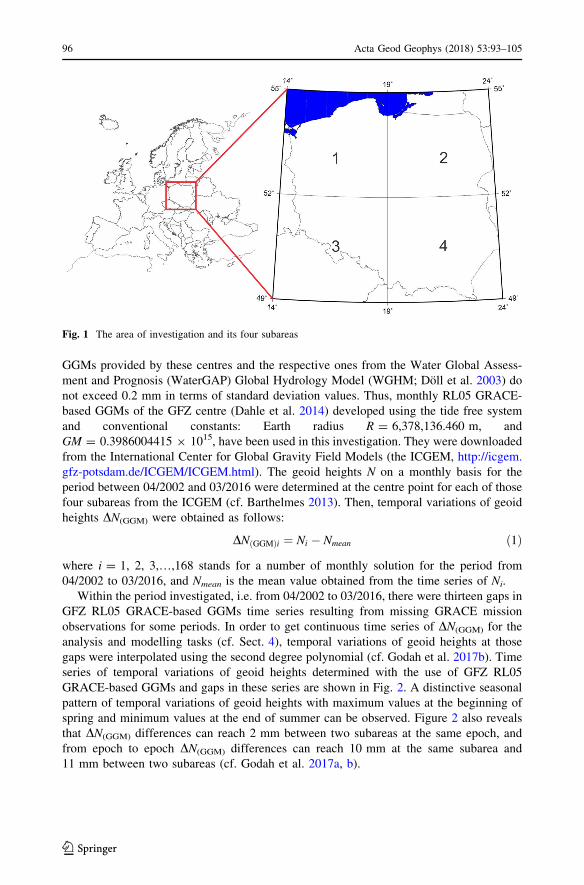
The area of Poland, bounded by the parallels of 49�N and 55�N and the meridians of 14�Eand 24�E, has been chosen as an investigation area. For this area the appropriate spatial
resolution of RL05 GRACE-based GGMs filtered using the decorrelation (DDK3; see
Kusche et al. 2009) filter and truncated at degree/order 60 is about 3� 9 3� (Godah et al.
2017a). Thus, the area of the investigation has been divided into four subareas (Fig. 1).
Moreover, Godah et al. (2017a) revealed that temporal variations of geoid heights obtained
from RL05 GRACE-based GGMs developed by the CSR and JPL centres over the area of
Poland are very similar to the corresponding ones of the GeoForschungsZentrum (GFZ)
centre. The differences between temporal variations of geoid heights calculated from
Acta Geod Geophys (2018) 53:93–105 95
123
GGMs provided by these centres and the respective ones from the Water Global Assess-
ment and Prognosis (WaterGAP) Global Hydrology Model (WGHM; Doll et al. 2003) do
not exceed 0.2 mm in terms of standard deviation values. Thus, monthly RL05 GRACE-
based GGMs of the GFZ centre (Dahle et al. 2014) developed using the tide free system
and conventional constants: Earth radius R = 6,378,136.460 m, and
GM = 0.3986004415 9 1015, have been used in this investigation. They were downloaded
from the International Center for Global Gravity Field Models (the ICGEM, http://icgem.
gfz-potsdam.de/ICGEM/ICGEM.html). The geoid heights N on a monthly basis for the
period between 04/2002 and 03/2016 were determined at the centre point for each of those
four subareas from the ICGEM (cf. Barthelmes 2013). Then, temporal variations of geoid
heights DN(GGM) were obtained as follows:
DNðGGMÞi ¼ Ni � Nmean ð1Þ
where i = 1, 2, 3,…,168 stands for a number of monthly solution for the period from
04/2002 to 03/2016, and Nmean is the mean value obtained from the time series of Ni.
Within the period investigated, i.e. from 04/2002 to 03/2016, there were thirteen gaps in
GFZ RL05 GRACE-based GGMs time series resulting from missing GRACE mission
observations for some periods. In order to get continuous time series of DN(GGM) for the
analysis and modelling tasks (cf. Sect. 4), temporal variations of geoid heights at those
gaps were interpolated using the second degree polynomial (cf. Godah et al. 2017b). Time
series of temporal variations of geoid heights determined with the use of GFZ RL05
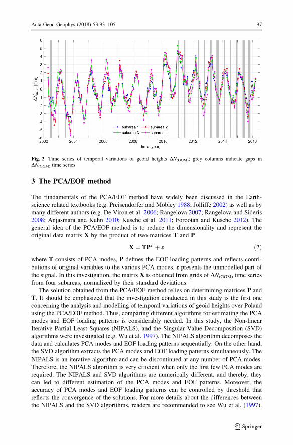
GRACE-based GGMs and gaps in these series are shown in Fig. 2. A distinctive seasonal
pattern of temporal variations of geoid heights with maximum values at the beginning of
spring and minimum values at the end of summer can be observed. Figure 2 also reveals
that DN(GGM) differences can reach 2 mm between two subareas at the same epoch, and
from epoch to epoch DN(GGM) differences can reach 10 mm at the same subarea and
11 mm between two subareas (cf. Godah et al. 2017a, b).
Fig. 1 The area of investigation and its four subareas
96 Acta Geod Geophys (2018) 53:93–105
123
3 The PCA/EOF method
The fundamentals of the PCA/EOF method have widely been discussed in the Earth-
science related textbooks (e.g. Preisendorfer and Mobley 1988; Jolliffe 2002) as well as by
many different authors (e.g. De Viron et al. 2006; Rangelova 2007; Rangelova and Sideris
2008; Anjasmara and Kuhn 2010; Kusche et al. 2011; Forootan and Kusche 2012). The
general idea of the PCA/EOF method is to reduce the dimensionality and represent the
original data matrix X by the product of two matrices T and P
X ¼ TPT þ e ð2Þ
where T consists of PCA modes, P defines the EOF loading patterns and reflects contri-
butions of original variables to the various PCA modes, e presents the unmodelled part of
the signal. In this investigation, the matrix X is obtained from grids of DN(GGM) time series
from four subareas, normalized by their standard deviations.
The solution obtained from the PCA/EOF method relies on determining matrices P and
T. It should be emphasized that the investigation conducted in this study is the first one
concerning the analysis and modelling of temporal variations of geoid heights over Poland
using the PCA/EOF method. Thus, comparing different algorithms for estimating the PCA
modes and EOF loading patterns is considerably needed. In this study, the Non-linear
Iterative Partial Least Squares (NIPALS), and the Singular Value Decomposition (SVD)
algorithms were investigated (e.g. Wu et al. 1997). The NIPALS algorithm decomposes the
data and calculates PCA modes and EOF loading patterns sequentially. On the other hand,
the SVD algorithm extracts the PCA modes and EOF loading patterns simultaneously. The
NIPALS is an iterative algorithm and can be discontinued at any number of PCA modes.
Therefore, the NIPALS algorithm is very efficient when only the first few PCA modes are
required. The NIPALS and SVD algorithms are numerically different, and thereby, they
can led to different estimation of the PCA modes and EOF patterns. Moreover, the
accuracy of PCA modes and EOF loading patterns can be controlled by threshold that
reflects the convergence of the solutions. For more details about the differences between
the NIPALS and the SVD algorithms, readers are recommended to see Wu et al. (1997).
Fig. 2 Time series of temporal variations of geoid heights DN(GGM); grey columns indicate gaps inDN(GGM) time series
Acta Geod Geophys (2018) 53:93–105 97
123
The algorithms are described shortly in this paper as follows (e.g. Wold et al. 1987;
Cordella 2012):
The NIPALS algorithm is an iterative procedure to estimate PCA modes and EOF
loading patterns. The vector t contains PCA modes while the vector p contains loadings.
The convergence criterion, which is constant in the procedure, e.g. threshold = 10-4, is
set.
The following steps are performed in the NIPALS algorithm:
1. Set up t as the column from X, e.g. with the largest variance.
2. Project X onto t to calculate the corresponding loading p
p ¼ XTt
tTt
3. Normalize loading vector p to length 1
p ¼ pffiffiffiffiffiffiffiffi
pTpp
4. Project X onto p to calculate the corresponding new vector t
t ¼ XTp
pTp
5. Check the convergence. If the difference between snew = (tTt) and sold (from last
iteration) is larger than threshold*snew return to step 2.
6. Remove the estimated PCA mode and EOF loading pattern from X:
E ¼ X� tpT
7. In order to estimate other PCA modes and EOF loading patterns repeat the procedure
from the step 1 using the obtained matrix E as the X.
The SVD algorithm is based on a theorem from linear algebra, in which a rectangular
matrix X is decomposed into the product of three new matrices:
X ¼ USVT
where columns of U are orthonormal eigenvectors of XXT, columns of V are orthonormal
eigenvectors of XTX, S is a diagonal matrix containing singular values of X, i.e. square
roots of eigenvalues from U or V in decreasing order. The column vectors of V define the
EOF loading patterns. The PCA modes are obtained from the column vectors of the matrix
T = US.
The computation steps of the SVD algorithm are as follows:
1. Compute XT, XTX.
2. Compute eigenvalues of XTX and sort them in descending order along its diagonal by
resolving
XTX� kI�
�
�
� ¼ 0
3. Compute the square root of eigenvalues of XTX to obtain the singular values of X.
4. Build a diagonal matrix S by sorting singular values in descending order along its
diagonal and compute S-1.
98 Acta Geod Geophys (2018) 53:93–105
123
5. Use eigenvalues from step 2 in descending order and compute the eigenvectors of
XTX. Place these eigenvectors along the columns of V.
6. Compute U = XVS-1 and compute PCA modes T = US.
In this study, the NIPALS algorithm has been employed using the STATISTICA
software (http://www.statsoft.pl/), whilst the SVD algorithm has been implemented with
the use of the MATLAB software, in particular, the function ‘‘pca’’ (https://www.
mathworks.com/help/stats/pca.html).
The percentages of the total variance of temporal variations of geoid heights r(total) were
estimated as follows:
rðtotalÞk ¼ kkD2
ð3Þ
where kk denotes the eigenvalue estimated from the matrix X, k is the number of the PCA
mode and variable D is the total variance of temporal variations of geoid heights.
4 Results
4.1 Analysis of temporal geoid height variations
With the use of the PCA/EOF method, temporal variations of geoid heights obtained from
RL05 GRACE-based GGMs for four subareas and normalized by their standard deviations
were analysed. The percentages of the total variance of temporal variations of geoid
heights reflected by three PCA modes are given in Table 1. They reveal that, over the area
of the investigation, *99.93% of DN(GGM) variance can be obtained using the first three
PCA modes and EOF loading patterns. The first PCA/EOF accounts for the most signif-
icant variance of these variations, i.e. *96.4%. The second and third PCA/EOF reflect less
than 3.5% of total variance of temporal variations of geoid heights over the area
investigated.
Figure 3 shows the first three PCA modes and their corresponding EOF loading patterns
of temporal variations of geoid heights over the area of Poland. The first PCA mode reveals
a clear seasonal pattern of temporal variations of geoid heights, with maximum values in
March and minimum values in July–September. This seasonal pattern is strongly correlated
with the increases/decreases of water masses over the area investigated, which are due to
the melting of snow that had been accumulated in the winter season, and the water
evaporation during dry months within the summer season (cf. Krynski et al. 2014; Godah
et al. 2017a, b). Figure 3 also shows that the first EOF loading pattern ranges from
*0.8526 to *1.0741. It indicates very similar loading patterns of temporal variations of
geoid heights obtained for all four subareas. This is because the characteristics of DN(GGM)
are very similar, i.e. at the same epoch DN(GGM) differences between subareas do not
exceed 2 mm, for all four subareas (see Fig. 2).
Table 1 The total variance reflected by the first three PCA modes [%]
PCA mode SVD algorithm NIPALS algorithm
1 96.42 96.33
2 2.11 2.21
3 1.40 1.38
Acta Geod Geophys (2018) 53:93–105 99
123
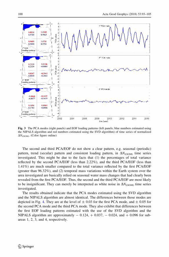
The second and third PCA/EOF do not show a clear pattern, e.g. seasonal (periodic)
pattern, trend (secular) pattern and consistent loading pattern, in DN(GGM) time series
investigated. This might be due to the facts that (1) the percentages of total variance
reflected by the second PCA/EOF (less than 2.22%), and the third PCA/EOF (less than
1.41%) are much smaller compared to the total variance reflected by the first PCA/EOF
(greater than 96.32%), and (2) temporal mass variations within the Earth system over the
area investigated are basically relied on seasonal water mass changes that had clearly been
revealed from the first PCA/EOF. Thus, the second and the third PCA/EOF are most likely
to be insignificant. They can merely be interpreted as white noise in DN(GGM) time series
investigated.
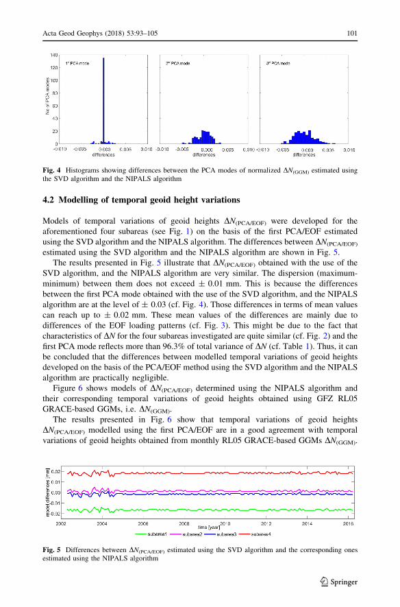
The results obtained indicate that the PCA modes estimated using the SVD algorithm
and the NIPALS algorithm are almost identical. The differences between those modes are
depicted in Fig. 4. They are at the level of ± 0.03 for the first PCA mode, and ± 0.05 for
the second PCA mode and the third PCA mode. They also exhibit that differences between
the first EOF loading patterns estimated with the use of the SVD algorithm and the
NIPALS algorithm are approximately - 0.124, ? 0.037, - 0.024, and ? 0.096 for sub-
areas 1, 2, 3, and 4, respectively.
Fig. 3 The PCA modes (right panels) and EOF loading patterns (left panels; blue numbers estimated usingthe NIPALS algorithm and red numbers estimated using the SVD algorithm) of time series of normalizedDN(GGM). (Color figure online)
100 Acta Geod Geophys (2018) 53:93–105
123
4.2 Modelling of temporal geoid height variations
Models of temporal variations of geoid heights DN(PCA/EOF) were developed for the
aforementioned four subareas (see Fig. 1) on the basis of the first PCA/EOF estimated
using the SVD algorithm and the NIPALS algorithm. The differences between DN(PCA/EOF)
estimated using the SVD algorithm and the NIPALS algorithm are shown in Fig. 5.
The results presented in Fig. 5 illustrate that DN(PCA/EOF) obtained with the use of the
SVD algorithm, and the NIPALS algorithm are very similar. The dispersion (maximum-
minimum) between them does not exceed ± 0.01 mm. This is because the differences
between the first PCA mode obtained with the use of the SVD algorithm, and the NIPALS
algorithm are at the level of ± 0.03 (cf. Fig. 4). Those differences in terms of mean values
can reach up to ± 0.02 mm. These mean values of the differences are mainly due to
differences of the EOF loading patterns (cf. Fig. 3). This might be due to the fact that
characteristics of DN for the four subareas investigated are quite similar (cf. Fig. 2) and the
first PCA mode reflects more than 96.3% of total variance of DN (cf. Table 1). Thus, it can
be concluded that the differences between modelled temporal variations of geoid heights
developed on the basis of the PCA/EOF method using the SVD algorithm and the NIPALS
algorithm are practically negligible.
Figure 6 shows models of DN(PCA/EOF) determined using the NIPALS algorithm and
their corresponding temporal variations of geoid heights obtained using GFZ RL05
GRACE-based GGMs, i.e. DN(GGM).
The results presented in Fig. 6 show that temporal variations of geoid heights
DN(PCA/EOF) modelled using the first PCA/EOF are in a good agreement with temporal
variations of geoid heights obtained from monthly RL05 GRACE-based GGMs DN(GGM).
Fig. 4 Histograms showing differences between the PCA modes of normalized DN(GGM) estimated usingthe SVD algorithm and the NIPALS algorithm
Fig. 5 Differences between DN(PCA/EOF) estimated using the SVD algorithm and the corresponding onesestimated using the NIPALS algorithm
Acta Geod Geophys (2018) 53:93–105 101
123
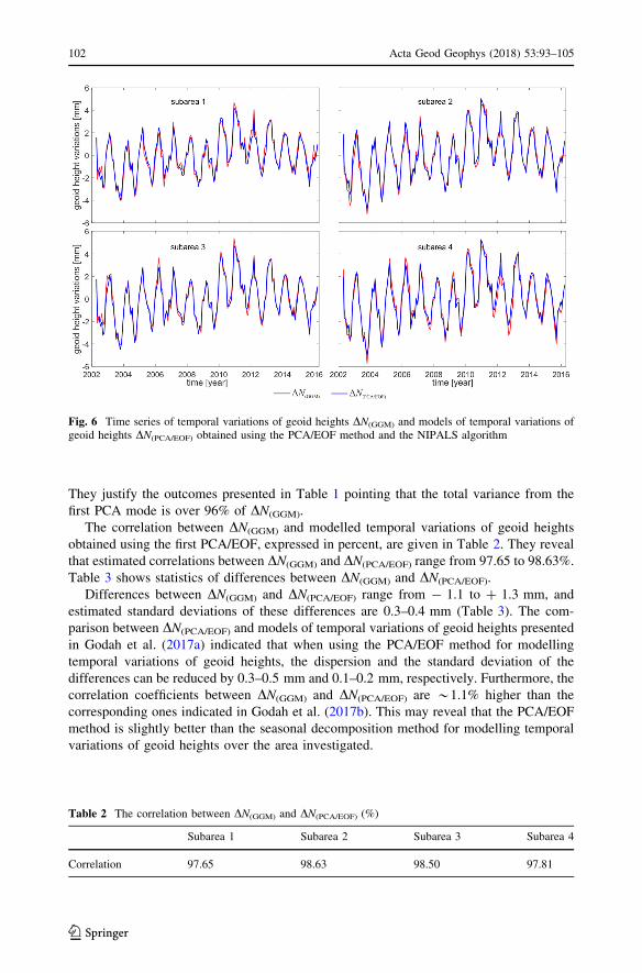
They justify the outcomes presented in Table 1 pointing that the total variance from the
first PCA mode is over 96% of DN(GGM).
The correlation between DN(GGM) and modelled temporal variations of geoid heights
obtained using the first PCA/EOF, expressed in percent, are given in Table 2. They reveal
that estimated correlations between DN(GGM) and DN(PCA/EOF) range from 97.65 to 98.63%.
Table 3 shows statistics of differences between DN(GGM) and DN(PCA/EOF).
Differences between DN(GGM) and DN(PCA/EOF) range from - 1.1 to ? 1.3 mm, and
estimated standard deviations of these differences are 0.3–0.4 mm (Table 3). The com-
parison between DN(PCA/EOF) and models of temporal variations of geoid heights presented
in Godah et al. (2017a) indicated that when using the PCA/EOF method for modelling
temporal variations of geoid heights, the dispersion and the standard deviation of the
differences can be reduced by 0.3–0.5 mm and 0.1–0.2 mm, respectively. Furthermore, the
correlation coefficients between DN(GGM) and DN(PCA/EOF) are *1.1% higher than the
corresponding ones indicated in Godah et al. (2017b). This may reveal that the PCA/EOF
method is slightly better than the seasonal decomposition method for modelling temporal
variations of geoid heights over the area investigated.
Fig. 6 Time series of temporal variations of geoid heights DN(GGM) and models of temporal variations ofgeoid heights DN(PCA/EOF) obtained using the PCA/EOF method and the NIPALS algorithm
Table 2 The correlation between DN(GGM) and DN(PCA/EOF) (%)
Subarea 1 Subarea 2 Subarea 3 Subarea 4
Correlation 97.65 98.63 98.50 97.81
102 Acta Geod Geophys (2018) 53:93–105
123
5 Conclusions
This paper discusses the analysis and modelling of temporal variations of geoid heights
over the area of Poland using the Principal Component Analysis/Empirical Orthogonal
Function (PCA/EOF) method. Temporal variations of geoid heights DN for the period from
04/2002 to 03/2016 over the area of Poland divided into four subareas of 3� 9 5� were
determined from GRACE mission data. The DN can reach 10 mm at the same subarea and
11 mm between two subareas. These DN variations should be considered when deter-
mining the orthometric height using the ellipsoid heights from GNSS data for different
seasons. They should also be considered to improve the static quasigeoid model developed
over the area of Poland, which currently fit to GNSS/levelling data with the accuracy of
14–22 mm, in terms of the standard deviation of the differences.
Two algorithms: the Singular Value Decomposition (SVD) algorithm and the Non-
linear Iterative Partial Least Squares (NIPALS) algorithm, were implemented to estimate
the PCA modes and their corresponding EOF loading patterns.
The results revealed that *99.93% of total variance of temporal variations of geoid
heights can be obtained using the first three PCA modes and EOF loading patterns. The
significant signal, i.e. greater than 96.3% in terms of total variance, of temporal variations
of geoid heights over the area of Poland can be obtained from the first PCA mode and EOF
loading pattern.
Models of temporal variations of geoid heights developed using the PCA/EOF
method are satisfactory. The fit, in terms of standard deviations of differences between
temporal variations of geoid height models DN(PCA/EOF) obtained with the use of the
PCA/EOF method, and the respective ones determined from RL05 GRACE-based GGMs
DN(GGM) is of 0.3–0.4 mm. The DN(PCA/EOF) values are highly correlated, i.e.
97.65–98.63%, with the DN(GGM).
Overall, the PCA/EOF method is recommended for modelling temporal variations of
geoid heights over the area of Poland. It provides slightly better results compared to other
methods implemented so far over the area investigated, i.e. the Fourier analysis and the
seasonal decomposition methods. The differences between DN(GGM) and DN(PCA/EOF)
obtained when implementing the SVD algorithm, and the NIPALS algorithm do not exceed
± 0.01 mm. They are practically negligible.
Acknowledgement This work was supported by the Polish National Science Centre (NCN) within theresearch Grant No. 2014/13/B/ST/10/02742. The two anonymous reviewers are cordially appreciated fortheir constructive comments on the manuscript.
Open Access This article is distributed under the terms of the Creative Commons Attribution 4.0 Inter-national License (http://creativecommons.org/licenses/by/4.0/), which permits unrestricted use, distribution,
Table 3 Statistics of the differ-ences between DN
(GGM)and
DN(PCA/EOF)
(mm)
Subarea DN(GGM) - DN(PCA/EOF)
Min Max Mean SD
1 - 0.8 1.1 0.0 0.4
2 - 1.1 0.8 0.0 0.3
3 - 0.9 1.3 0.0 0.3
4 - 1.1 1.1 0.0 0.4
Acta Geod Geophys (2018) 53:93–105 103
123
and reproduction in any medium, provided you give appropriate credit to the original author(s) and thesource, provide a link to the Creative Commons license, and indicate if changes were made.
References
Anjasmara IM, Kuhn M (2010) Analysing five years of grace equivalent water height variations using theprincipal component analysis. In: Mertikas SP (ed) Gravity, geoid and earth observation. InternationalAssociation of Geodesy Symposia vol 135, pp 547–555. doi:10.1007/978-3-642-10634-7_73
Barthelmes F (2013) Definition of functionals of the geopotential and their calculation from sphericalharmonic models theory and formulas used by the calculation service of the International centre forglobal earth models (ICGEM). The GFZ series, Scientific technical report (STR), STR 09/02, Revisededition Jan 2013, p 32
Barthelmes F (2016) International centre for global earth models (ICGEM). J Geod 90(10):1177–1180 [In:Drewes H, Kuglitsch F, Adam J, Rozsa S (eds) The geodesists handbook 2016. J Geod90(10):907–1205]
Bloomfield P (2000) Fourier analysis of time series: an introduction, 2nd edn. Wiley, New YorkCordella C (2012) PCA: the basic building block of chemometrics. Analytical chemistry. In: Krull IS (ed)
InTech. doi:10.5772/51429. https://www.intechopen.com/books/analytical-chemistry/pca-the-basic-building-block-of-chemometrics
Dahle C, Flechtner F, Gruber C et al. (2014) GFZ RL05: an improved time-series of monthly GRACEgravity field solutions. In: Flechtner F, Sneeuw N, Schuh W-D (eds) Observation of the system earthfrom space—CHAMP, GRACE, GOCE and future missions. Advanced technologies in earth sciences.GEOTECHNOLOGIEN Science report no. 20, pp 29–39. doi:10.1007/978-3-642-32135-1_4
De Viron O, Panet I, Diament M (2006) Extracting low frequency climate signal from GRACE data. eEarthDiscuss 1(1):21–36. https://hal.archives-ouvertes.fr/hal-00330772/
Doll P, Kaspar F, Lehner B (2003) A global hydrological model for deriving water availability indicators:model tuning and validation. J Hydrol 270(1–2):105–134
Drewes H, Kuglitsch F, Adam J, Rozsa S (2016) The geodesist’s handbook 2016. J Geod 90(10):907–1205.doi:Doi.org/10.1007/s00190-016-0948-z
Forootan E, Kusche J (2012) Separation of global time-variable gravity signals into maximally independentcomponents. J Geod 86(7):477–497. doi:10.1007/s00190-011-0532-5
Godah W, Szelachowska M, Krynski J (2017a) On the analysis of temporal geoid height variations obtainedfrom GRACE-based GGMs over the area of Poland. Acta Geophys 65(4):713–725. doi:10.1007/s11600-017-0064-3
Godah W, Szelachowska M, Krynski J (2017b) Investigation of geoid height variations and vertical dis-placements of the earth surface in the context of the realization of the modern vertical referencesystem: a case study for Poland. International association of geodesy symposia. Springer, Berlin,Heidelberg. https://doi.org/10.1007/1345_2017_15
Jolliffe I (2002) Principal component analysis. Springer-Verlag, New YorkKrynski J (2007) Precise quasigeoid modelling in Poland—results and accuracy estimation (in Polish).
Monographic series of the Institute of Geodesy and Cartography, No 13, Warsaw, Poland, p 266Krynski J, Kloch-Głowka G, Szelachowska M (2014) Analysis of time variations of the gravity field over
Europe obtained from GRACE data in terms of geoid height and mass variations. In: Rizos C, Willis P(eds) Earth on the edge: science for a sustainable planet. International Association of Geodesy Sym-posia, vol 139, pp 365–370. doi:10.1007/978-3-642-37222-3_48
Kusche J, Schmidt R, Petrovic S, Rietbroek R (2009) Decorrelated GRACE time-variable gravity solutionsby GFZ, and their validation using a hydrological model. J Geod 83(10):903–913. doi:10.1007/s00190-009-0308-3
Kusche J, Eicker A, Forootan E (2011) Analysis tools for GRACE and related data sets, theoretical basis.Presented at: Mass transport and mass distribution in the system earth, Mayschoss, Germany, 12–16Sept 2011. In: Eicker A, Kusche J (eds) Lecture notes from the summer school of DFG SPP1257 globalwater cycle: the international geoscience programme (IGCP)
Makridakis S, Wheelwright SC, McGee VE (1983) Forecasting: methods and applications, 2nd edn. Wiley,New York
Preisendorfer RW, Mobley CD (1988) Principal component analysis in meteorology and oceanography.Elsevier, Amsterdam
Rangelova E (2007) A dynamic geoid model for Canada. Ph.D. Thesis, University of Calgary, Departmentof Geomatics Engineering, Report No. 20261
104 Acta Geod Geophys (2018) 53:93–105
123
Rangelova E, Sideris MG (2008) Contributions of terrestrial and GRACE data to the study of the seculargeoid changes in North America. J Geodyn 46(3):131–143
Rangelova E, Fotopoulos G, Sideris MG (2010) Implementing a dynamic geoid as a vertical datum fororthometric heights in Canada. In: Mertikas SP (ed) Gravity, geoid and earth observation. InternationalAssociation of Geodesy Symposia vol 135, pp 295–302. doi:10.1007/978-3-642-10634-7_38
Szelachowska M, Krynski J (2014) GDQM-PL13—the new gravimetric quasigeoid model for Poland.Geoinf Issues 1(6):5–19
Tapley BD, Bettadpur S, Watkins M, Reigber C (2004) The gravity recovery and climate experiment:mission overview and early results. Geophys Res Lett 31:L09607. doi:10.1029/2004GL019920
Wold S, Esbensen K, Geladi P (1987) Principal component analysis. Chemom Intell Lab Syst 2(1–3):37–52Wu W, Massarat DL, de Jong S (1997) The kernel PCA algorithms for wide data. Part I: theory and
algorithms. Chemom Intell Lab Syst 36(2):165–172. doi:10.1016/S0169-7439(97)00010-5
Acta Geod Geophys (2018) 53:93–105 105
123


![ANALISIS EMPIRICAL ORTHOGONAL FUNCTION (EOF) BERBASIS ... · metode EOF dilanjutkan oleh Kutzbach [2] menggunakan tiga peubah iklim dalam analisis EOF, yaitu SPL, suhu permukaan,](https://img.pdfslide.net/doc/110x75/60969947efe15d0f8310cce9/analisis-empirical-orthogonal-function-eof-berbasis-metode-eof-dilanjutkan.jpg)