1

ESS210B

Prof. Jin-Y

i Yu

Part 4: T

ime Series II

EO

F Analysis

Principal Com

ponent

Rotated E

OF

Singular Value

Decom

position (SVD

)

ESS210B

Prof. Jin-Y

i Yu

Em

pirical Orthogonal Function A

nalysis

Em

pirical Orthogonal Function (E

OF) analysis attem

pts to find a relatively sm

all number of independent variables

(predictors; factors) which convey as m

uch of the original inform

ation as possible without redundancy.

EO

F analysis can be used to explore the structure of the variability w

ithin a data set in a objective way, and to

analyze relationships within a set of variables.

EO

F analysis is also called principal component analysis

or factor analysis.

ESS210B

Prof. Jin-Y

i Yu

What D

oes EO

F Analysis do?

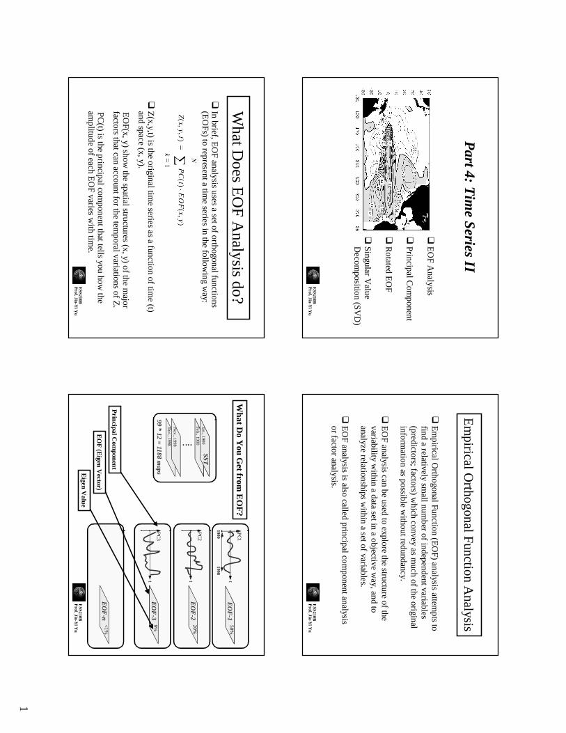
In brief, EO

F analysis uses a set of orthogonal functions (E

OFs) to represent a tim

e series in the following w

ay:

Z(x,y,t) is the original tim

e series as a function of time (t)

and space (x, y).

EO

F(x, y) show the spatial structures (x, y) of the m

ajor factors that can account for the tem

poral variations of Z.

PC(t) is the principal com

ponent that tells you how the

amplitude of each E

OF varies w

ith time.

ESS210B

Prof. Jin-Y

i Yu

EO

F-1

50%

PC

1

t

19001998

EO

F-2

20%t

PC

2

EO

F-3

••••

9%t

PC

3

EO

F-n

<1%

Feb., 1900

Dec., 1998 •••

Nov., 1998 •

Jan., 1900SST

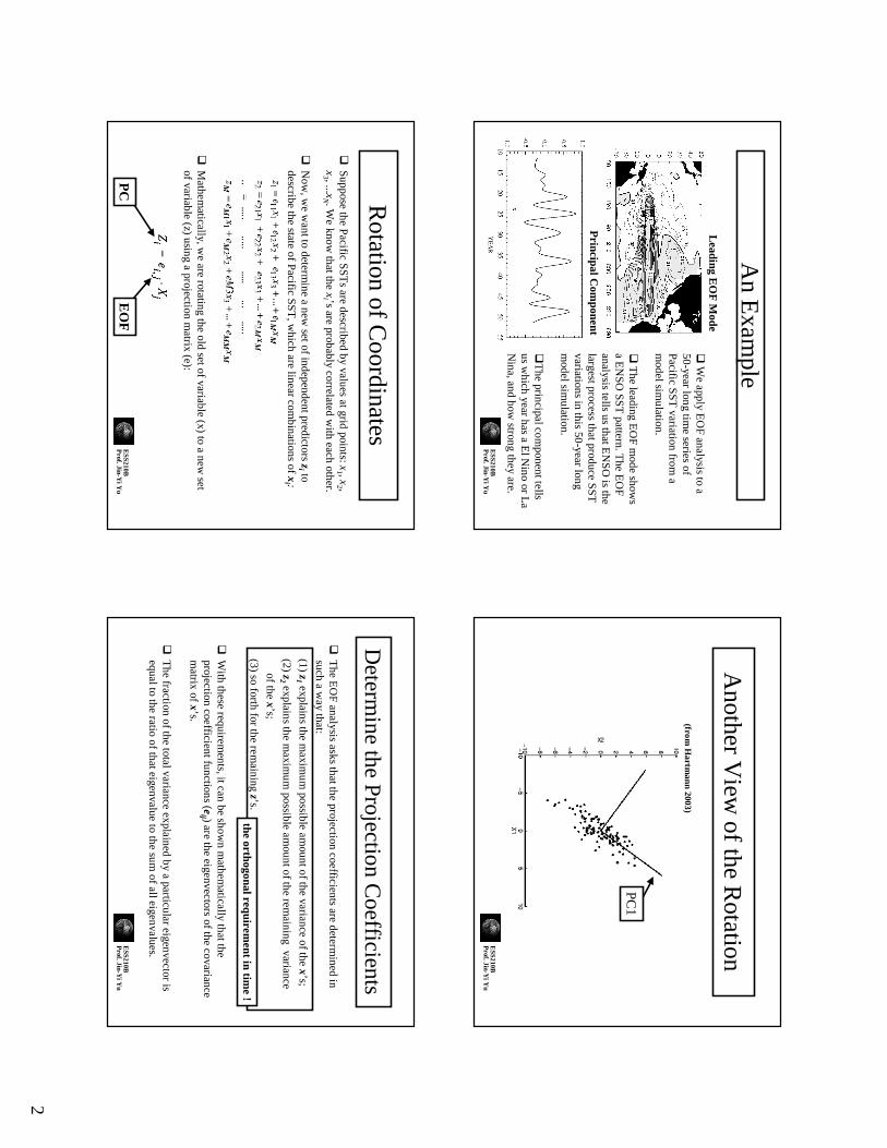
99 * 12 = 1188 maps

EO

F

Analysis

Principal C

omponent

EO

F (E

igen Vector)

Eigen V

alue

What D

o You G

et from E

OF

?

2

ESS210B

Prof. Jin-Y

i Yu

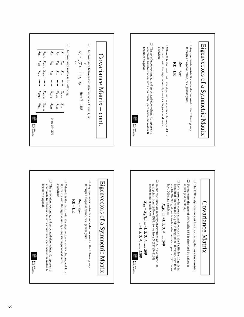
An E

xample

Principal C

omponent

Leading E

OF

Mode

We apply E

OF analysis to a

50-year long time series of

Pacific SST

variation from a

model sim

ulation.

The leading E

OF m

ode shows

a EN

SO SS

T pattern. T

he EO

F analysis tells us that E

NS

O is the

largest process that produce SST

variations in this 50-year long m

odel simulation.

The principal com

ponent tells us w

hich year has a El N

ino or La

Nina, and how

strong they are.

ESS210B

Prof. Jin-Y

i Yu

Another V

iew of the R

otation

(from H

artmann 2003)

PC

1

ESS210B

Prof. Jin-Y

i Yu

Rotation of C

oordinates Suppose the Pacific S

STs are described by values at grid points:x

1 , x2 ,

x3 , ...x

N . We know

that thex

i ’s are probably correlated with each other.

Now

, we w

ant to determine a new

set of independent predictors zi to

describe the state of Pacific SST

, which are linear com

binationsof x

i :

Mathem

atically, we are rotating the old set of variable (x) to a

new set

of variable (z) using a projection matrix (e):

PC

EO

FE

SS210BP

rof. Jin-Yi Y

u

Determ

ine the Projection Coefficients

The E

OF analysis asks that the projection coefficients are determ

ined in such a w

ay that:

(1)z

1explains the m

aximum

possible amount of the variance of the x’s;

(2) z2

explains the maxim

um possible am

ount of the remaining variance

of the x’s;

(3) so forth for the remaining z’s.

With these requirem

ents, it can be shown m

athematically that the

projection coefficient functions (eij ) are the eigenvectors of the covariance

matrix of x’s.

The fraction of the total variance explained by a particular eigenvector is

equal to the ratio of that eigenvalueto the sum

of all eigenvalues.

the orthogonal requirement in tim

e !

3

ESS210B

Prof. Jin-Y

i Yu

Eigenvectors of a Sym

metric M

atrix

Any sym

metric m

atrix R can be decom

posed in the following w

ay through a

diagonalization, or eigenanalysis:

Where E

is the matrix w

ith the eigenvectorse

i as its columns, and L

is the m

atrix with the

eigenvalues λi , along its diagonal and zeros

elsewhere.

The set of eigenvectors,e

i , and associatedeigenvalues,λ

i , represent a coordinate transform

ation into a coordinate space where the m

atrix R

becomes diagonal.

ESS210B

Prof. Jin-Y

i Yu

Covariance M

atrixT

he EO

F analysis has to start from calculating the covariance m

atrix.

For our case, the state of the Pacific SST

is described by values at m

odel grid points Xi .

Let’s assum

e the observational network in the Pacific has 10 grids in

latitudinal direction and 20 grids in longitudinal direction, then there are 10x20=

200 grid points to describe the state of pacific SST. S

o we

have 200 state variables:

Xm (t), m

=1, 2, 3, 4, …, 200

In our case, there are monthly observations of SST

s over these 200 grid points from

1900 to 1998. So w

e have N (12*99=

1188) observations at each X

m:

Xm

n=

Xm (tn ), m

=1, 2, 3, 4, …., 200

n=1, 2, 3, 4, ….., 1188

ESS210B

Prof. Jin-Y

i Yu

Covariance M

atrix –cont.

The covariance betw

een two state variables X

i and Xj is:

The covariance m

atrix is as following:

Here N

= 1188

X12

X1,M

-1X

1MX

11X

13•••••

X22

X2,M

-1X

2,MX

21X

23•••••

X32

X3,M

-1X

3,MX

31X

33•••••

XM

-1,2X

M-1,M

-1X

M-1,M

XM

-1,1X

M-1,3

•••••X

M,2

XM

,M-1

XM

,MX

M,1

XM

,3•••••

Here M

= 200

ESS210B

Prof. Jin-Y

i Yu

Eigenvectors of a Sym

metric M

atrix

Any sym

metric m

atrix R can be decom

posed in the following w

ay through a

diagonalization, or eigenanalysis:

Where E

is the matrix w

ith the eigenvectorse

i as its columns, and L

is the m

atrix with the

eigenvalues λi , along its diagonal and zeros

elsewhere.

The set of eigenvectors,e

i , and associatedeigenvalues,λ

i , represent a coordinate transform

ation into a coordinate space where the m

atrix R

becomes diagonal.

4

ESS210B

Prof. Jin-Y

i Yu

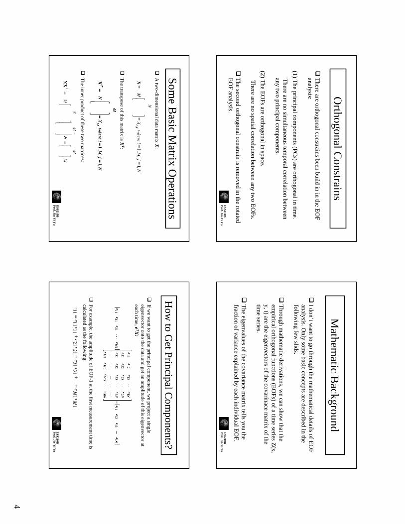
Orthogonal C

onstrains

There are orthogonal constrains been build in in the E

OF

analysis:

(1)T

he principal components (PC

s) are orthogonal in time.

There are no sim

ultaneous temporal correlation betw

een any tw

o principal components.

(2) The E

OFs are orthogonal in space.

There are no spatial correlation betw

een any two E

OFs.

The second orthogonal constrain is rem

oved in the rotated E

OF analysis.

ESS210B

Prof. Jin-Y

i Yu

Mathem

atic Background

I don’t want to go through the m

athematical details of E

OF

analysis. Only som

e basic concepts are described in the follow

ing few slids.

Through m

athematic derivations, w

e can show that the

empirical orthogonal functions (E

OFs) of a tim

e series Z(x,

y, t) are the eigenvectors of the covarinace matrix of the

time series.

The eigenvalues

of the covariance matrix tells you the

fraction of variance explained by each individual EO

F.

ESS210B

Prof. Jin-Y

i Yu

Some B

asic Matrix O

perationsA

two-dim

ensional data matrix X

:

The transpose of this m

atrix is XT:

The inner product of these tw

o matrices:

ESS210B

Prof. Jin-Y

i Yu

How

to Get P

rincipal Com

ponents?

If we w

ant to get the principal component, w

e project a single eigenvector onto the data and get an am

plitude of this eigenvector at each tim

e, eTX

:

For example, the am

plitude of EO

F-1 at the first m

easurement tim

e is calculated as the follow

ing:

5

ESS210B

Prof. Jin-Y

i Yu

Using SV

D to G

et EO

F&P

C

We can use Singular V

alue Decom

position (SVD

) to get E

OFs,eigenvalues, and PC

’s directly from the data m

atrix, w

ithout the need to calculate the covariance matrix from

the data first.

If the data set is relatively small, this m

ay be easier than com

puting the covariance matrices and doing the

eigenanalysisof them

.

If the sample size is large, it m

ay be computationally m

ore efficient to use the

eigenvaluem

ethod.

ESS210B

Prof. Jin-Y

i Yu

What is SV

D?

Any m

by n matrix A

can be factored into

The colum

ns of U (m

by m) are the E

OFs

The colum

ns of V (n by n) are the P

Cs.

The diagonal values of Σ

are the eigenvalues represent the amplitudes

of the EO

Fs, but not the variance explained by the EO

F.

The square of the eigenvalue from

the SVD

is equal to the eigenvalue from

the eigen analysis of the covariance matrix.

original time series

EO

Fs

normalized P

Cs

ESS210B

Prof. Jin-Y

i Yu

An E

xample –

with SV

D m

ethod

(from H

artmann 2003)

ESS210B

Prof. Jin-Y

i Yu

An E

xample –

With E

igenanalysis

(from H

artmann 2003)

6

ESS210B

Prof. Jin-Y

i Yu

Correlation M

atrixSom

etime, w

e use the correlation matrix, in stead of the covariance

matrix, for E

OF analysis.

For the same tim

e series, the EO

Fsobtained from

the covariance m

atrix will be different from

the EO

Fs obtained from the correlation

matrix.

The decision to choose the covariance m

atrix or the correlation matrix

depends on how w

e wish the variance at each grid points (X

i ) are w

eighted.

In the case of the covariance matrix form

ulation, the elements of the

state vector with larger variances w

ill be weighted m

ore heavily.

With the correlation m

atrix, all elements receive the sam

e weight and

only the structure and not the amplitude w

ill influence the principal com

ponents.E

SS210BP

rof. Jin-Yi Y

u

Correlation M

atrix –cont.

The correlation m

atrix should be used for the following

two cases:

(1)The state vector is a com

bination of things with different

units.

(2) The variance of the state vector varies from

point to point so m

uch that this distorts the patterns in the data.

ESS210B

Prof. Jin-Y

i Yu

Presentations of EO

F –V

ariance Map

There are several w

ays to present EO

Fs. T

he simplest w

ay is to plot the values of E

OF itself. T

his presentation can not tell you howm

uch the real am

plitude this EO

F represents.

One w

ay to represent EO

F’s amplitude is to take the tim

e series of principal com

ponents for an EO

F, normalize this tim

e series to unit variance, and then regress it against the original data set.

This m

ap has the shape of the EO

F, but the amplitude actually

corresponds to the amplitude in the real data w

ith which this structure

is associated.

If we have other variables, w

e can regress them all on the PC

ofone

EO

F and show the structure of several variables w

ith the correctam

plitude relationship, for example, S

ST and surface vector w

indfields can both be regressed on PC

s of SST.

ESS210B

Prof. Jin-Y

i Yu

Presentations of EO

F –C

orrelation Map

Another w

ay to present EO

F is to correlate the principal com

ponent of an EO

F with the original tim

e series at each data point.

This w

ay, present the EO

F structure in a correlation map.

In this way, the correlation m

ap tells you what are the co-

varying part of the variable (for example, SST

) in the spatial dom

ain.

In this presentation, the EO

F has no unit and is non-dim

ensional.

7

ESS210B

Prof. Jin-Y

i Yu

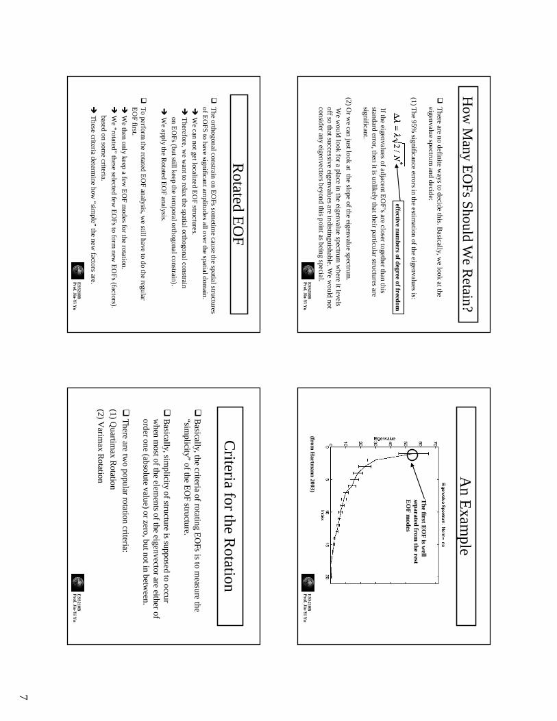
How

Many E

OF

s Should W

e Retain?

There are no definite w

ays to decide this. Basically, w

e look atthe eigenvalue spectrum

and decide:

(1)The 95%

significance errors in the estimation of the eigenvalues is:

If theeigenvalues

of adjacent EO

F’s are closer together than this standard error, then it is unlikely that their particular structures are significant.

(2) Or w

e can just look at the slope of the eigenvalue spectrum.

We w

ould look for a place in theeigenvalue

spectrum w

here it levels off so that successive eigenvalues

are indistinguishable. We w

ould not consider any eigenvectors beyond this point as being special.

effective numbers of degree of freedom

ESS210B

Prof. Jin-Y

i Yu

An E

xample

The first E

OF

is well

separated from the rest

EO

F m

odes

(from H

artmann 2003)

ESS210B

Prof. Jin-Y

i Yu

Rotated E

OF

The orthogonal constrain on E

OFs

sometim

e cause the spatial structures of E

OFS

to have significant amplitudes all over the spatial dom

ain.

We can not get localized E

OF structures.

Therefore, w

e want to relax the spatial orthogonal constrain

on EO

Fs (but still keep the temporal orthogonal constrain).

We apply the R

otated EO

F analysis.

To perform

the rotated EO

F analysis, we still have to do the regular

EO

F first.

We then only keep a few

EO

F modes for the rotation.

We “rotated”

these selected few E

OF

s to form new

EO

Fs (factors).

based on some criteria.

These criteria determ

ine how “sim

ple”the new

factors are.

ESS210B

Prof. Jin-Y

i Yu

Criteria for the R

otation

Basically, the criteria of rotating E

OFs

is to measure the

“simplicity”

of the EO

F structure.

Basically, sim

plicity of structure is supposed to occur w

hen most of the elem

ents of the eigenvector are either of order one (absolute value) or zero, but not in betw

een.

There are tw

o popular rotation criteria:

(1)Q

uartimax

Rotation

(2)V

arimax

Rotation

8

ESS210B

Prof. Jin-Y

i Yu

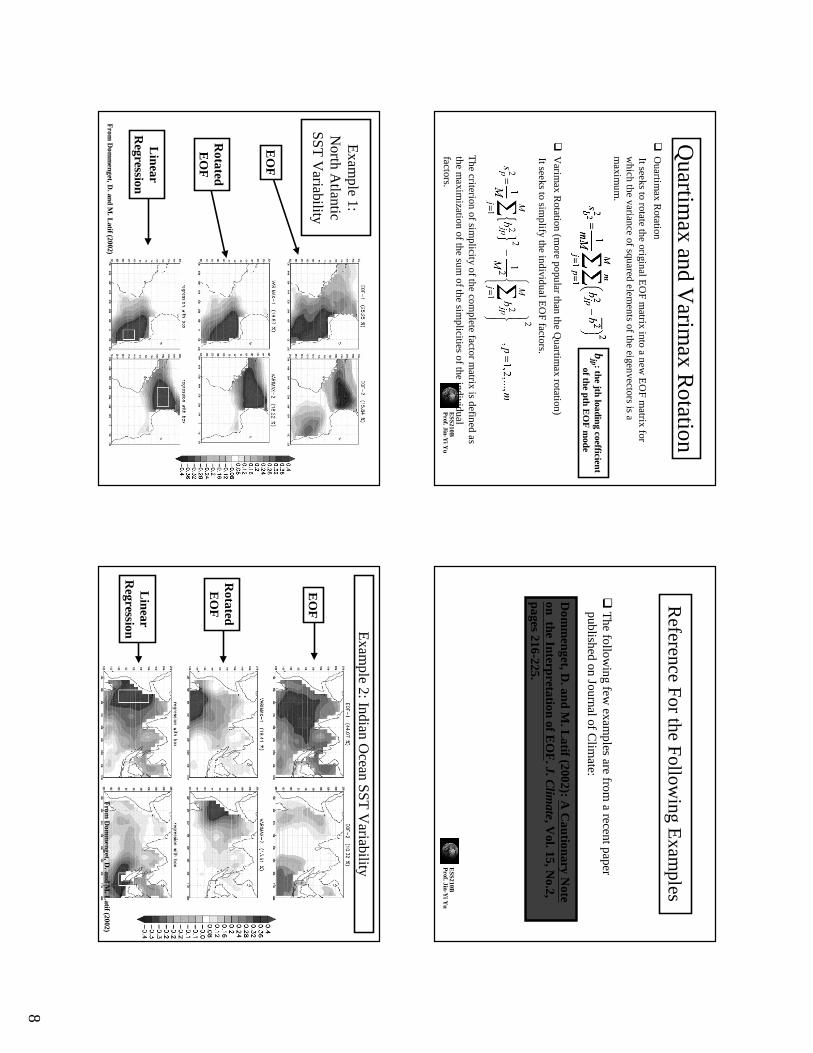
Quartim

ax and Varim

ax Rotation

Ouartim

axR

otation

It seeks to rotate the original EO

F matrix into a new

EO

F matrix for

which the variance of squared elem

ents of the eigenvectors is a m

aximum

.

Varim

ax Rotation (m

ore popular than the Quartim

ax rotation)

It seeks to simplify the individual E

OF factors.

The criterion of sim

plicity of the complete factor m

atrix is defined as the m

aximization of the sum

of the simplicities of the individual

factors.

bjp : the jth loading coefficient

of the pth EO

F m

ode

ESS210B

Prof. Jin-Y

i Yu

Reference F

or the Follow

ing Exam

ples

The follow

ing few exam

ples are from a recent paper

published on Journal of Clim

ate:

Dom

menget, D

. and M.L

atif(2002): A

Cautionary N

ote on

the Interpretation of EO

F. J. C

limate, V

ol. 15, No.2,

pages 216-225.

ESS210B

Prof. Jin-Y

i Yu

Exam

ple 1:N

orth Atlantic

SST V

ariability

RotatedE

OF

Linear

Regression

EO

F

From

Dom

menget, D

. and M.L

atif(2002)E

SS210BP

rof. Jin-Yi Y

u

Exam

ple 2: Indian Ocean SST

Variability

RotatedE

OF

Linear

Regression

EO

F

From

Dom

menget, D

. and M.L

atif(2002)

9

ESS210B

Prof. Jin-Y

i Yu

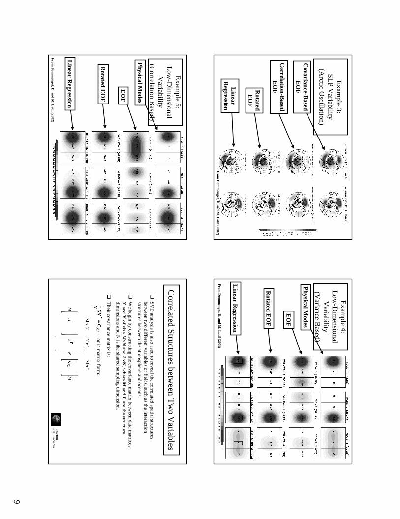
Exam

ple 3:SL

P Variability

(Arctic O

scillation)

RotatedE

OF

Linear

Regression

Covariance-B

asedE

OF

Correlation-B

asedE

OF

From

Dom

menget, D

. and M.L

atif(2002)E

SS210BP

rof. Jin-Yi Y

u

Exam

ple 4:L

ow-D

imensional

Variability

(Variance B

ased)

Rotated E

OF

Linear R

egression

Physical M

odes

EO

F

From

Dom

menget, D

. and M.L

atif(2002)

ESS210B

Prof. Jin-Y

i Yu

Exam

ple 5:L

ow-D

imensional

Variability

(Correlation B

ased)

Rotated E

OF

Linear R

egression

Physical M

odes

EO

F

From

Dom

menget, D

. and M.L

atif(2002)E

SS210BP

rof. Jin-Yi Y

u

Correlated S

tructures between T

wo V

ariables

SVD

analysis is also used to reveal the correlated spatial structures betw

een two different variables or fields, such as the interaction

structures between the atm

osphere and oceans.

We begin by constructing the covariance m

atrix between data m

atrices X

and Y of size

MxN

andL

xN, w

here Mand L

are the structure dim

ensions and N is the shared sam

pling dimension.

Their covariance m

atrix is:

or in matrix form

:

10

ESS210B

Prof. Jin-Y

i Yu

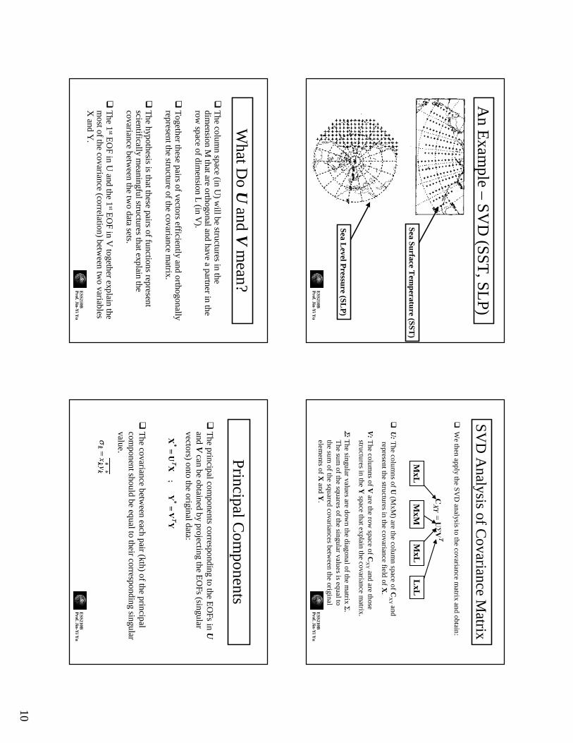
An E

xample –

SV

D (SST

, SLP)

Sea Surface Tem

perature (SST)

Sea Level P

ressure (SLP

)

ESS210B

Prof. Jin-Y

i Yu

SV

D A

nalysis of Covariance M

atrix

We then apply the S

VD

analysis to the covariance matrix and obtain:

U:

The colum

ns of U(M

xM) are the colum

n space of CX

Y and

represent the structures in the covariance field of X.

V:

The colum

ns of V are the row

space of CX

Yand are those

structures in the Y space that explain the covariance m

atrix.

Σ:

The singular values are dow

n the diagonal of the matrix Σ

. T

he sum of the squares of the singular values is equalto

the sum of the squared covariances

between the original

elements of X

and Y.

MxL

MxM

MxL

LxL

ESS210B

Prof. Jin-Y

i Yu

What D

o Uand V

mean?

The colum

n space (in U) w

ill be structures in the dim

ension M that are orthogonal and have a partner in the

row space of dim

ension L (in V

).

Together these pairs of vectors efficiently and

orthogonallyrepresent the structure of the covariance m

atrix.

The hypothesis is that these pairs of functions represent

scientifically meaningful structures that explain the

covariance between the tw

o data sets.

The 1

stEO

F in U and the 1

stEO

F in V together explain the

most of the covariance (correlation) betw

een two variables

X and Y

.E

SS210BP

rof. Jin-Yi Y

u

Principal Com

ponents

The principal com

ponents corresponding to the EO

Fs in Uand V

can be obtained by projecting the EO

Fs (singular vectors) onto the original data:

The covariance betw

een each pair (kth) of the principal com

ponent should be equal to their corresponding singular value.

11

ESS210B

Prof. Jin-Y

i Yu

Presentation of SV

D V

ectorsSim

ilar to the EO

S analysis, the singular vectors are norm

alizedand

non-dimensional, w

hereas the expansion coefficients have the dim

ensions of the original data.

To include am

plitude information in the singular vectors, w

e canregress (ore correlate) the principal com

ponents of U or V

with the

original data for this purpose.

(1) For example, norm

alize the principal component of U

.

(2) Regress this norm

alized principal component w

ith the original data set Y

to produce a “heterogeneous regression map”. T

his map show

s the am

plitude of covariance between X

and Y.

(3) Regress this norm

alized principal component w

ith the original data set X

to produce a “homogeneous m

ap”. This m

ap tells us the spatial structure of X

that is most correlated w

ith Y.

ESS210B

Prof. Jin-Y

i Yu

Heterogeneous and H

omogeneous M

aps

Heterogeneous regression m

aps: regress (or correlate) the expansion coefficient tim

e series of the left field with the input data for the right

field, or do the same w

ith the expansion coefficient time series

for the right field and the input data for the left field.

Hom

ogeneous regression maps: regress (or correlate) the expansion

coefficient time series of the left field w

ith the input data for the left field, or do the sam

e with the right field and its expansion coefficients.

ESS210B

Prof. Jin-Y

i Yu

An E

xample –

SV

D (SST

, SLP)

Sea Surface Tem

perature (SST)

Sea Level P

ressure (SLP

)

ESS210B

Prof. Jin-Y

i Yu

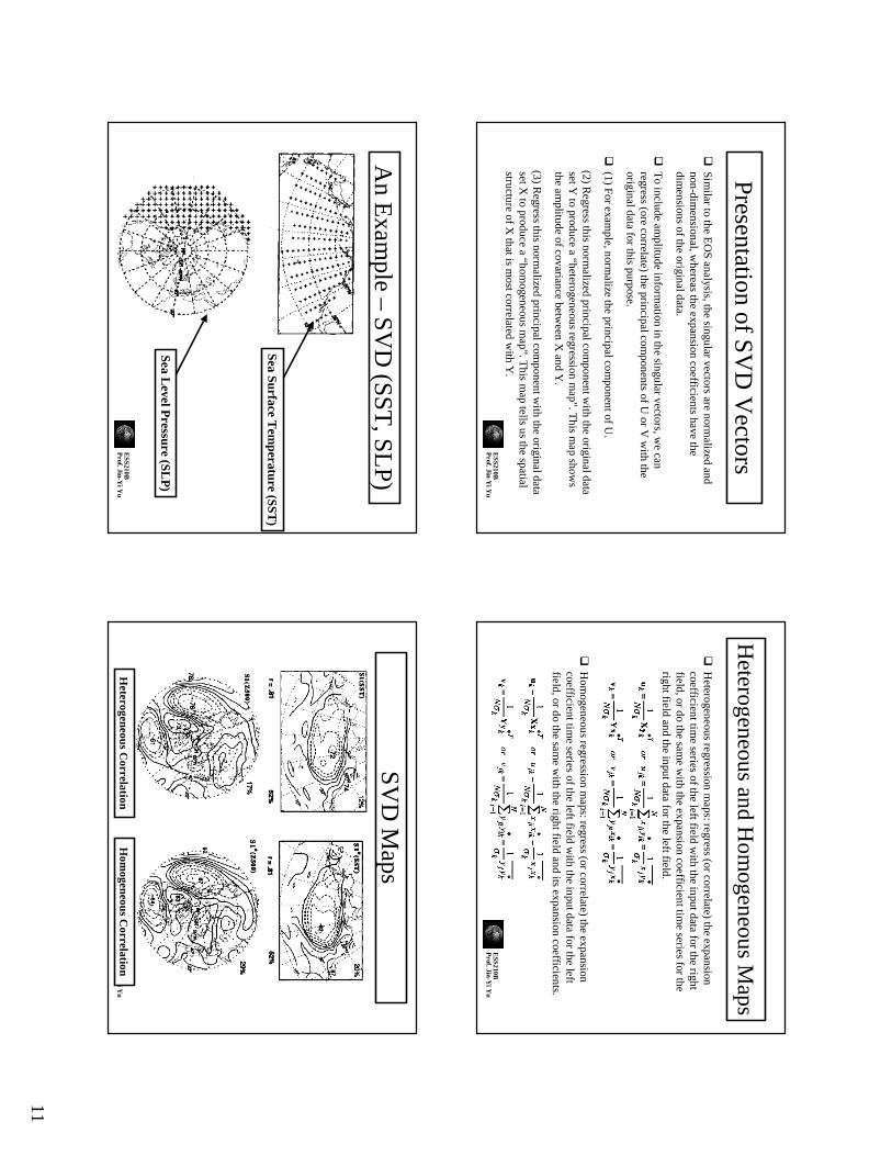
SVD

Maps

Heterogeneous C

orrelationH

omogeneous C

orrelation

12

ESS210B

Prof. Jin-Y

i Yu

How

to Use M

atlab to do SVD

?

See pages 27-28 of the paper “A m

anual for E

OF and SV

D analysis of clim

ate data”by

Bjornsson

and Venegas.