Application of the Probabilistic Dynamic Synthesis Method to Realistic

Structures

Andrew M. Brown*

NASA Marshall Space Flight Center, Huntsville, AL 35812

Aldo A. Ferri +

Georgia Institute of Technology, Atlanta, GA 30332

Abstract

The Probabilistic Dynamic Synthesis method is a technique Ibr obtaining the

statistics of a desired response engineering quantity for a structure with non-deterministic

parameters. The method uses measured data from modal testing of the structure as the

input random variables, rather than more "primitive" quantities like geometry or material

variation. This modal information is much more comprehensive and easily measured than

the "primitive" information. The probabilistic analysis is carried out using either response

surface reliability methods or Monte Carlo simulation. In previous work, the feasibility of

the PDS method applied to a simple seven degree-of-freedom spring-mass system was

verified. In this paper, extensive issues involved with applying the method to a realistic

three-substructure system are examined, and free and forced response analyses are

performed. The results from using the method are promising, especially when the lack of

alternatives for obtaining quantitative output for probabilistic structures is considered.

Nomenclature

shortest distance from the g=O curve to the origin

"Aerospace Engineer, Structural Dynamics and Loads Branch, Structural Analysis Division, ED23, MSFC,AL 35812, Member AIAA+Associate Professor, Woodruff School of Mechanical Engineering, Georgia Tech, Atlanta, GA 30332,Member AIAA

https://ntrs.nasa.gov/search.jsp?R=19990041443 2018-08-29T06:26:01+00:00Z

[C] a

CDF

CMS

dof's

_(.)

FORM

[Gbb] m,i

g

{ _,}m,i

[_]m,i

PDS

p(Y<y )

MC

rv

U

{x}

{x} °

Xo

Xi

Xo

X

X*

Y(X)

Correlation matrix of rv's in substructure, a

cumulative distribution function

component mode synthesis

degrees of freedom

Gaussian CDF function

First Order Reliability Method

residual flexibility matrix

limit state function

eigenvalues

eigenvectors

probabilistic dynamic synthesis

the probability that Y is less than y

Monte Carlo

random variable

vector of uncorrelated std. normal rv's

vector of correlated normal rv's

vector of correlated std. normal rv's

median of x

boundary dot's

internal dot's

internal dof's with applied load

vector of random variables

design or most probable point (MPP)

performance function

Introduction

Accountingfor thestatisticalgeometricandmaterialvariabilityof structuresin

analysishasbeenatopicof considerableresearchfor thelast30years.Thedetermination

of quantifiablemeasuresof statisticalprobabilityof adesiredresponsevariable,suchas

naturalfrequency,maximumdisplacement,orstress,to replaceexperience-based"safety

factors"hasbeenaprimarygoalof thisresearch.Thereareseveralproblemsassociated

with its satisfactoryapplicationto realisticstructures,though.Thefirst problem is

accuratedefinitionof theinputrandomvariables(rv's).Therandomvariabilityof the

materialcharacteristicsis generallyavailable,butthevariationin thegeometryof acomplex

structure,suchasahollowed-outturbineblade,isvirtually impossibleto defineaccurately.

Thesecondproblemfor analysisis the largesizeof thefiniteelementmodelsfrequently

usedto simulatethesestructures.Substructuringreductiontechniquesarerequiredto

decreasethesizeof manystructuralsystemsjust to performasingle,deterministicanalysis.

Finally,asignificantproblemin theanalysisof probabilisticstructuresis theaccurate

generationof theCumulativeDistributionFunction(CDF)necessaryto obtainthe

probabilityof thedesiredresponsevariable.MonteCarlo(MC) simulationscanbe

performedto calculateprobabilitydistributionsof thedesiredoutput,butseveralthousand

runsarerequiredfor accurateresults.

Thisresearchappliesamethodologypreviouslydevelopedby the authors,called

"probabilisticdynamicsynthesis"(PDS)to solvetheseproblemst. ThePDSmethoduses

dynamiccharacteristicsof substructuresmeasuredfrom modaltestastheinputrandom

variablesratherthan"primitive"randomvariablessuchasmaterialandgeometricvariability.

Thesecharacteristics,which are the free-freeeigenvalues,eigenvectors,andresidual

flexibility, arereadilymeasuredandfor manysubstructures,areasonablesamplesetof

thesemeasurementscanbeobtained.Thevariationin thesedynamicattributesaccurately

accountsfor theentirerandomvariabilityof thesubstructure.This is in contrastto using

"primitive" rv's, whichnomatterhow well measured,cannotcapturethevariationof every

geometricgridpointlocationin additionto thevariationin materialproperties.Usingthe

residualflexibility methodof componentmodesynthesis(CMS),thesedynamic

characteristicsareusedto generatesamplemodelsof thesubstructuresthatarecoupledto

form samplesystemmodels,whichareconsiderablysmallerthananunreducedfinite

elementmodel. Finally,thesesamplemodelsareusedto obtaintheCDFof theresponse

variablebyeitherapplyingMonteCarlosimulationorby generatingdatapointsfor usein

theresponsesurfacereliabilitymethod,whichsavesasubstantialamountof computertime.

Thepreviousworkbytheauthorsverifiedthefeasibilityof thePDSmethodona

simplesevendegree-of-freedom(dot')spring-masssystem.In thispaper,weexaminethe

extensiveissuesinvolvedwithapplyingthemethodto arealistically-modeledthree

substructuresystem.Bothfreeresponseandforcedresponseanalysesareperformed.The

goalof thefree-responseanalysisis to quantifya+/- 3_ band about the median natural

frequency, compared to the somewhat arbitrary +/- 5% band about the deterministic

solution frequently used in industry. The goal of the forced response analysis is to quantify

a + 3ty value for the maximum response of a dof on the structure, compared with the

completely experience-based "factor of safety" presently applied to the maximum

responding dof in a deterministic analysis. These results are presented by comparing a

CDF obtained using a Monte Carlo simulation of the "baseline" model, in which "primitive"

random variables are used, with a CDF using the PDS method. While there is considerable

room for improvement, these results are promising, especially when existing options for

design of realistic structures are considered. Finally, potential sources of error and avenues

of further research are presented.

Probabilistic Background

The research described in this paper employs the response surface reliability method

approach of probabilistic structural mechanics for determining the statistical structural

response characteristics. A more extensive review of the reliability methods is presented

4

by Brown2. To briefly reviewthistechnique,considera limit statefunctiong(X) = Y(X) -

y,wherey is specificvalue.Comell3,andHasover& Lind4developedtheFirst Order

ReliabilityMethod(FORM)by dividingtheX spaceinto twoparts,g < O (Y < y) andg >

O (Y > y), andapproximatinggasafirst orderTaylor seriesexpandedaboutthemeanof

eachrv.

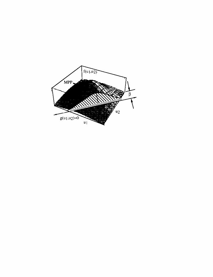
If X is transformedto independentstandardnormalrv's U, thenthis first order

approximationallowsthemulti-dimensionalprobabilitydensityfunction(PDF)to be

representedby aonedimensionalGaussianPDF(seeFig. 1).Therefore,P(Y< y) ---_(13),

where_(.) is theGaussianCDF functionfoundin handbooks,and[3is shortestdistance

from theg=Ocurveto theorigin,locatedat theMostProbablePoint(MPP). This greatly

simplifiesthecalculationof probabilityvaluesfor agivenlimit state.Thereliabilitymethod

wasexpandedbyRackwitz5to multi-dimensionalproblemsfor whichthelimit statecurve

g=Ois anexplicit,nonlinearfunctionof therv's,whichmakesthedeterminationof [3much

moredifficult. Themethodmakesuseof Lagrangetechniquesin an iterative algorithmto

find [3.Rackwitz& Feissler6andChen& Lind7continuedthedevelopmentof thismethod

by examininghowto developan"equivalentnormaldistribution"for rv'swith non-normal

distributions.

Theapplicationof FORM anditsextensionsfor non-explicitlimit statefunctions,as

is thecasefor largestructuralfiniteelementmodels,requirestheuseof numerical

differentiationto obtainafirst orderapproximationof theperformancefunctionY(X). A

CDFcanbeconstructedfrom this first orderapproximationusingthetechniquedescribed

aboveordirectlyfromthefirst orderapproximationsof themeanandstandarddeviationif

thedistributionis assumedto beGaussian.A practicalsecondorderapproachwas

developedin 1987by Wu & Wirshing8,whoimprovedtheaccuracyof probabilitylevels

obtainedby FORM for non-explicitlimit statesby usingapartialsecondorderexpansion

calledtheAdvancedFORM (AFORM). Initially, theFORM is performedandMPP's

obtained.Thelimit stateis thenexpandedabouteachMPPusingonly thefirst orderand

5

thepure(nomixedvariableterms)secondordertermsof theTaylor seriesexpansion.The

first andsecondordertermsarethen"linearized"usingachangeof variable,andtheMPP

searchalgorithmusedin FORM isapplied. A CDFcanalsobegenerateddirectlyfrom this

partial secondorderapproximationif a lognormaldistributionis assumed.Wu also

developedtheAdvancedMeanValue(AMV) method,aprocedurefor updatingtheFORM

or AFORMsolutionby usingtheoriginal,exactsolutionfor g. All of thesereliability

methodshavebeenimplementedintoanewprobabilisticfinite-elementcomputercode

developedby SouthwestResearchInstitute,NESSUS 9.

System Description

In order to examine the applicability of the PDS method for a realistic design

problem, a structural system had to be chosen that met several criteria. First, the structure

had to be modeled using standard methodology. This was satisfied by using the widely

used commercial finite element code, NASTRAN. Next, since tying CMS together with

probabilistic methods is an important goal of this research, the size of the model had to be

large enough to be able to realize a substantial reduction in computer time due to dynamic

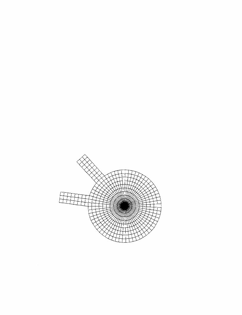
reduction. This requirement is satisfied by using a structural system composed of a "disk,"

which is made up of 630 quad4 plate elements and constrained at the center, and two

"blades," which are each composed of 24 quad4 plate elements (see Fig. 2). To pave the

way for future mistuned bladed-disk analyses, the disk was assumed to be deterministic and

the blades non-deterministic. For ease of analysis, the standard assumption that in-plane

translation and rotations are small has been applied. Finally, the structure had to possess a

"generic" level of randomness not easily defined by a single variation in a material or

geometric property. A single rv would not be able to capture variations in mode shapes that

are independent of variations of natural frequency, for instance. To achieve this goal, each

blade was separated into three sections, with two of the sections having a thickness set to be

an independent normally distributed primitive random variable. In addition, the density of

6

eachbladeacrossall threesectionswasdefinedasanormallydistributedindependentrv,

thus giving each bladethreeindependentrv's(seeTable1).

Monte Carlo Baseline Analysis

A Monte Carlo analysis of the original, unsubstructured system using the assumed

primitive random variable set was chosen to be a baseline for comparison with PDS. A

1000 sample case was executed, taking over 20 hours of wall-clock time. In addition, MC

analysis was required to simulate the modal testing phase of the PDS methodology to

obtain the statistics of the dynamic rv's of the probabilistic blade substructures. The

NESSUS computer code has a new interface with NASTRAN that manages the simulation,

both by creating the random vector set for the given input random variables, and by

automatically submitting the jobs. The input random variables can be any defined

NASTRAN geometric or material property.

Probabilistic Dynamic Synthesis

The PDS methodology makes use of the residual flexibility method of CMS. This

method has been developed by MacNeil 1°, Craig & Chang 11, and Martinez et al. _2. The

essential idea in CMS is that substructure modes are truncated since their higher modes will

not have a major effect on the combined system modes. The residual flexibility method

incorporates the effects of the higher modes by determining their flexibility. A side benefit

is that all the elements of the system stiffness matrix can be obtained from test and that the

mass matrix can be closely approximated by a unity matrix in the non-boundary partition.

Since all the information can be obtained from test, all the probabilistic information can be

incorporated into the system matrices for response analysis.

The first step of the probabilistic dynamic synthesis (PDS) method is to divide the

model of a structure into substructures m= a,b .... p, and the degrees of freedom into internal

and boundary locations. Each substructure is represented by n samples, each of which is

modallytestedin afreeinterfacecondition.For thisresearch,this testingstepissimulated

by aMC analysisof thestructureusingthedefinedprimitiverv's. Forsubstructurem,

samplei, thetestwill yieldeigenvalues{_,}m._andeigenvectors[O]m'i.Theeigenvectors

haveto beconsistentfrom onesampleto thenext,requiringaninterfacingFORTRANcode

to assignaconsistentsignto themodeshapesfor eachsampleandobtainingaconsistent

setof rigid-bodymodes(parallelto thecoordinatesystemaxes)for thetwo free-freemodes,

which isachievedbyusingtheSUPORTcardwith themodifiedHouseholdermethodin

NASTRAN. In addition,theboundarypartitionof theresidualflexibility matrix [Gbb] m'i is

obtained from the measured boundary drive point frequency response functions of the

boundary coordinates 13. Here, the residual flexibility is calculated analytically by

subtracting the flexibility for the retained modes from the total system flexibility (inverse of

the stiffness matrix) for the constrained substructure. For the free-free substructures, the

system is unconstrained so the stiffness matrix is singular. The "inertia-relief method,"

initially developed by Craig TM, is therefore used to obtain the residual flexibility.

For the free-response solution using the PDS method, only the kept (non-truncated)

eigenvalues, the boundary coordinates of the kept eigenvectors, and the boundary partition

of the residual flexibility matrix are needed. These values can be combined into a single

vector {x }m,i, defined as

T ] mAT

{X} m'i = [_l..._kl*bI1T ...{*b}k Oil ,.,Gbb ] (1)

where k is the number of kept modes. If the entire sample of substructure m is tested, {x }m

Can therefore be defined as a vector composed of elements that are each a random variable

with measured mean and standard deviation. This vector is now transformed to {x' }m a

vector of standard normally distributed rv's, using the measured mean and standard

deviation of each rv. An important assumption is made that the original rv's in {x } are

normally distributed. This distribution is required for decorrelation of the random

variables (discussed below), and is somewhat accurate, as shown in distribution-matching

testspublishedin thepreviousworkby theauthors1. If themeasureddistributionwere

foundtomatchanotherstandardtypebetter,thenancouldbeobtained.Sincethematch

with aGaussiandistributionis notperfect,though,thereis someerror introduced.A

techniqueto addressthiserror will bediscussedlaterin thispaper. Anothermethodof

increasingtheaccuracywouldbeto obtainan"equivalentnormal"distributionusingusing

theChen-Lindthree-parametermethod7 In addition, therewill be somedegreeof

correlationbetweeneachof therandomvariables,whichcanbecalculatedfrom the

measureddata.Thisinformationis placedin acorrelationmatrix [C]mrelatingeachelement

with everyotherelement. FortheFORManalysis,asetof independentrandomvariables

{ u }mis required. This can be accomplished by making an orthogonal transformation of

{x'}m with the eigenvectors of the correlation matrix to uncouple the {x'} coordinates,

thereby creating {u }m. This can be expressed for substructures m =a,b .... p as

{X'} m -- [CI)]c m {U} m (2)

It becomes evident at this time that the size of the dynamic rv set is intractable for a

realistic problem. For this case, which has only two probabilistic substructures and where

20 modes are retained (out of a possible 108) per substructure, the number of dynamic rv's

is 802. Several assumptions are therefore made to drastically reduce the number of

dynamic rv's. The first is to assume that the limit state function is insensitive to the variation

in the rotational dofs in the modes. This reduces the size of eigenvector rv's from 240 to 80

per substructure. The second is to assume the limit state is insensitive to not only the

rotational dofs, but also to the off-diagonal terms in the boundary residual flexibility matrix,

which reduces the size of that contribution from 144 to 4 per substructure. These

assumptions do not remove these variables from the formulation of the substructure

stiffness matrices; instead, it allows the use of the mean value of those variables (or median,

as will be discussed later). Admire, et. a115 examined the effect of completely removing the

9

off-diagonal G elements, and calculated a natural frequency error of less than 5% between

the exact value and the value obtained using the residual flexibility formulation.

In addition, a substantial reduction in the number of independent rv's is achieved by

eliminating "artificial" rv's. These were first found by calculating the correlation matrix of

the independent rv's [C]u. Since the elements of [C] u are uncorrelated, it was expected to be

an identity matrix. The result was somewhat different; for the rows/columns of [C] u that

corresponded to eigenvalues on the order of one, the diagonal term was equal to 1.0 and the

other elements in the associated row/column were very small. However, many of the

eigenvalues turned out to be very small and the analogous rows and columns in [C]u were

not diagonal; the diagonal values were 1.0 but the other terms in the row/column were all on

the order of one (between zero and one) instead of being close to zero. This can be

explained by realizing that the actual number of independent rv's in the system is equal to

the original number of independent primitive rv's, not the number of dynamic rv's.

Therefore, the rv's associated with the small _,c values are actually insignificant and the

magnitudes of these values are mainly due to numerical roundoff. The high off-diagonal

values in the new correlation matrix in these rows/columns therefore indicates a large

amount of correlation between these numerical artifact "rv's". The above result can be used

to further decrease the size of the rv set {u }. A sum of the eigenvalues of the original

correlation matrix is calculated, and any eigenvalue less than 3% of the sum is deemed

insignificant and the associated rv in {u} neglected. The value of 3% was reached by

starting at 5% and decreasing the cutoff value (thereby including more rv's) until the final

result stabilized. This reduced the eigenvalue set for each blade from 101 to 11. It is unclear

why this value did not actually reduce to three, which is the number of primitive rv's per

blade, but nevertheless, this reduction greatly facilitated the analysis.

To generate a first order Taylor series representation of the limit state, each

independent random variable is varied individually by some percentage of its standard

deviation c, which is equal to the square root of the corresponding eigenvalue of the

10

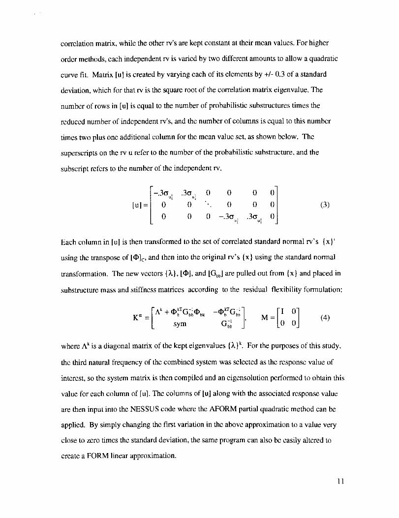
correlationmatrix,whiletheotherrv'sarekeptconstantat theirmeanvalues.Forhigher

ordermethods,eachindependentrv isvariedbytwo differentamountsto allowaquadratic

curvefit. Matrix [u] is createdbyvaryingeachof itselementsby +/- 0.3of a standard

deviation,whichfor thatrv is thesquarerootof thecorrelationmatrixeigenvalue.The

numberof rowsin [u] is equalto thenumberof probabilisticsubstructurestimesthe

reducednumberof independentrv's,andthenumberof columnsis equalto thisnumber

timestwoplusoneadditionalcolumnfor themeanvalueset,asshownbelow. The

superscriptson therv ureferto thenumberof theprobabilisticsubstructure,andthe

subscriptrefersto thenumberof theindependentrv.

-.3oo, .3Oul 0 0 0 i][u] = 0 0 "'. 0 0 (3)

0 0 0 -.3(rul .3Cul

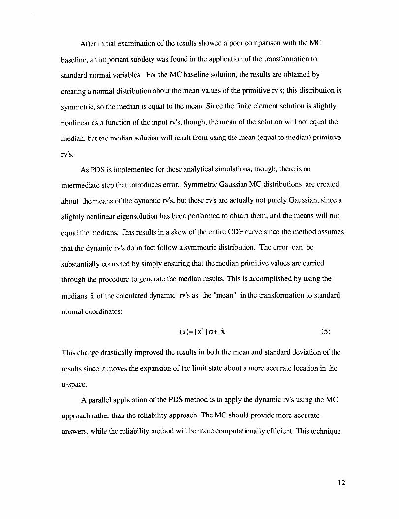
Each column in [u] is then transformed to the set of correlated standard normal rv's {x}'

using the transpose of [_]c, and then into the original rv's {x} using the standard normal

transformation. The new vectors {_}, [_], and [Gbb] are pulled out from {x} and placed in

substructure mass and stiffness matrices according to the residual flexibility formulation:

K s Ak "_ _b _bb=bk --_b _bb| 0= -1 ' M = (4)sym Gbb J 0

where A k is a diagonal matrix of the kept eigenvalues {_,}k. For the purposes of this study,

the third natural frequency of the combined system was selected as the response value of

interest, so the system matrix is then compiled and an eigensolution performed to obtain this

value for each column of [u]. The columns of [u] along with the associated response value

are then input into the NESSUS code where the AFORM partial quadratic method can be

applied. By simply changing the first variation in the above approximation to a value very

close to zero times the standard deviation, the same program can also be easily altered to

create a FORM linear approximation.

11

After initial examinationof theresultsshowedapoorcomparisonwith theMC

baseline,animportantsubtletywasfoundin theapplicationof thetransformationto

standardnormalvariables.FortheMC baselinesolution,theresultsareobtainedby

creatinganormaldistributionaboutthemeanvaluesof theprimitiverv's;thisdistributionis

symmetric,sothemedianisequaltothemean.Sincethefiniteelementsolutionis slightly

nonlinearasafunctionof theinputre's,though,themeanof thesolutionwill notequalthe

median,but themediansolutionwill resultfrom usingthemean(equaltomedian)primitive

rv's.

As PDS is implemented for these analytical simulations, though, there is an

intermediate step that introduces error. Symmetric Gaussian MC distributions are created

about the means of the dynamic re's, but these rv's are actually not purely Gaussian, since a

slightly nonlinear eigensolution has been performed to obtain them, and the means will not

equal the medians. This results in a skew of the entire CDF curve since the method assumes

that the dynamic rv's do in fact follow a symmetric distribution. The error can be

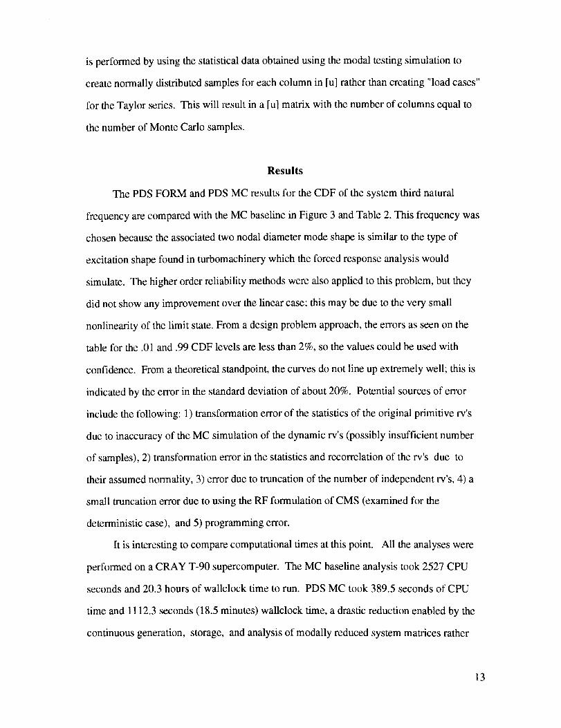
substantially corrected by simply ensuring that the median primitive values are carried

through the procedure to generate the median results. This is accomplished by using the

medians _ of the calculated dynamic

normal coordinates:

rv's as the "mean" in the transformation to standard

(x)={x'}_+ _ (5)

This change drastically improved the results in both the mean and standard deviation of the

results since it moves the expansion of the limit state about a more accurate location in the

u-space.

A parallel application of the PDS method is to apply the dynamic rv's using the MC

approach rather than the reliability approach. The MC should provide more accurate

answers, while the reliability method will be more computationally efficient. This technique

12

is performedbyusingthestatisticaldataobtainedusingthemodaltestingsimulationto

createnormallydistributedsamplesfor eachcolumnin [u] ratherthancreating"loadcases"

for theTaylor series.Thiswill resultin a[u] matrixwith thenumberof columnsequalto

thenumberof MonteCarlosamples.

Results

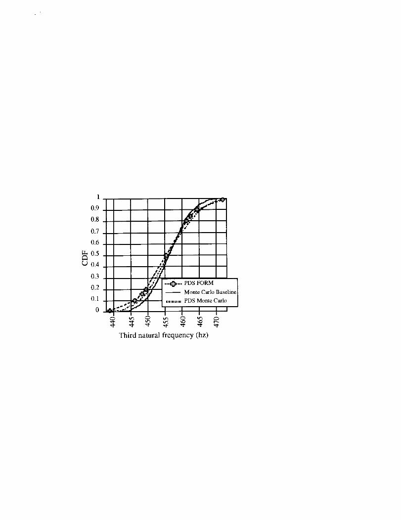
ThePDSFORM andPDSMC resultsfor theCDFof thesystemthird natural

frequencyarecomparedwith theMC baselinein Figure3 andTable2. This frequencywas

chosenbecausetheassociatedtwonodaldiametermodeshapeis similarto thetypeof

excitationshapefoundin turbomachinerywhichtheforcedresponseanalysiswould

simulate.Thehigherorderreliabilitymethodswerealsoappliedto thisproblem,but they

didnotshowanyimprovementoverthelinearcase;thismaybedueto theverysmall

nonlinearityof thelimit state.Fromadesignproblemapproach,theerrorsasseenon the

tablefor the.01and.99CDFlevelsarelessthan2%,sothevaluescouldbeusedwith

confidence.Fromatheoreticalstandpoint,thecurvesdonotline upextremelywell; thisis

indicatedbytheerrorin thestandarddeviationof about20%. Potentialsourcesof error

includethefollowing: 1)transformationerrorof thestatisticsof theoriginalprimitiverv's

dueto inaccuracyof theMC simulationof thedynamicrv's (possiblyinsufficientnumber

of samples),2) transformationerrorin thestatisticsandrecorrelationof therv's due to

theirassumednormality,3)errordueto truncationof thenumberof independentrv's,4) a

smalltruncationerrordueto usingtheRFformulationof CMS (examinedfor the

deterministiccase),and5) programmingerror.

It is interestingto comparecomputationaltimesat thispoint. All theanalyseswere

performedonaCRAY T-90supercomputer.TheMC baselineanalysistook 2527CPU

secondsand20.3hoursof wallclocktimeto run. PDSMC took389.5secondsof CPU

timeand1112.3seconds(18.5minutes)wallclocktime,adrasticreductionenabledbythe

continuousgeneration,storage,andanalysisof modallyreducedsystemmatricesrather

13

thanthecompletemodelgenerationandanalysisnecessaryfor eachof theMC baseline

samples.TheFORMmethodtook only 20.1secondsof CPUand64.2secondsof

wallclockto createthedatapointsfor inputto NESSUS,andabout30secondswallclockto

runNESSUSto performtheFORM solution.This furtherreductionis dueto the

substantialdecreasein thenumberof solutionsgenerated.As anticipated,boththeuseof

CMS andprobabilisticmethodsdrasticallydecreasedtheamountof timenecessaryto run

theanalysis,which,especiallyfor amoredetailedmodel,couldbeapre-requisitefor usein

design.

Forced Response

The use of PDS was now expanded to forced response. In particular, a frequency

response solution of the system was derived since this type of excitation would prove most

applicable to the bladed-disk problem. For forced response, the dofs of a substructure are

partitioned into three sections, xo, which are internal dofs with no external load applied, x_,

internal dof's with an external load applied, and x b, boundary dof's which may or may not

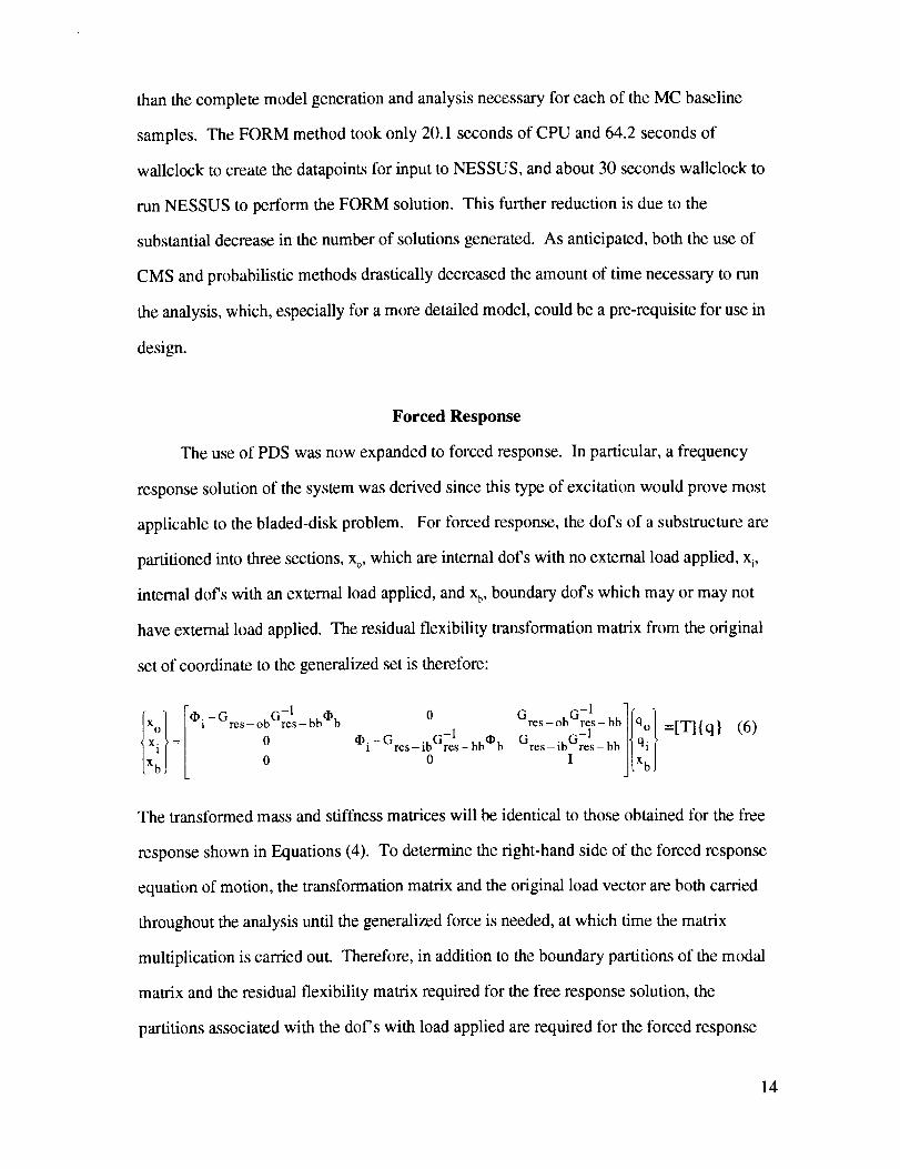
have external load applied. The residual flexibility transformation matrix from the original

set of coordinate to the generalized set is therefore:

ft[ i reob resb 0 reso a qoX°xi = 0 _.1 -Gres_ibGr-ls_ bb*b Gres-ibGrqs-bb/tqi t =[Tl{q} (6)

x b 0 0 I J[XbJ

The transformed mass and stiffness matrices will be identical to those obtained for the free

response shown in Equations (4). To determine the right-hand side of the forced response

equation of motion, the transformation matrix and the original load vector are both carried

throughout the analysis until the generalized force is needed, at which time the matrix

multiplication is carried out. Therefore, in addition to the boundary partitions of the modal

matrix and the residual flexibility matrix required for the free response solution, the

partitions associated with the doFs with load applied are required for the forced response

14

analysis.To moreeasilyperformthisanalysis,thetransformedcoupledsystemis

transformedto anuncoupledsystemusingthesetof truncatedmass-normalizedsystem

eigenvectors[_]1 resultingfrom thefreeresponsesolutionof thesystem,asshownbelow:

{q}l=[(I)]x{q]2 •

Theresultinguncoupledsystemis in theform

[I]{q}2 +[C]{q}2 +[A],{q}2 = [(I)]7[T]T{f}

(7)

(8)

where [A] 1is the diagonal matrix of the eigenvalues of the transformed system. The

standard (viscous) assumption of constant modal damping of 0.5% is used for [C]. The

input force is a system of four harmonic loads, each of amplitude 1 lb. (4.448 N) and

applied in-phase with a peak displacement of the two nodal diameter mode shape to simulate

bladed-disk excitation. There are standard techniques available for obtaining the frequency

response solution for this set of uncoupled single-dog systems. Because of the series of

linear transformations performed on the solution, though, a complex quantity for the

solution is desired rather than one in terms of magnitude and phase, as is commonly derived

in texts on the subject and which cannot be easily transformed. This complex vector {q }2

can now be transformed back to the original coordinates {x } using equations (6) and (7):

{x}=[T][(I)]l{q} 2 (9)

The absolute values of this complex vector are then calculated to obtain the physical

response values.

As seen above, applying PDS for the forced response solution requires more

information from the modal data and the residual flexibility matrices. This increases the

number of dynamic rv's necessary to solve the problem, which increases the complexity of

the problem in several aspects. To minimize this number, it is important to decide a-priori

which internal dot's will either have extemal load applied or require a displacement recovery.

Although the entire modal matrix and residual flexibility matrix are calculated, only those

15

partitionsof themodalmatrixandtheresidualflexibility matrix,alongwith theboundary

dofs,arestored.In addition,only thecorrelationswith theseadditionaldofs aregenerated.

To addressthedesignproblemdefinedearlier,theresponsevariablefor theforced

responseanalysiswaschosento bethemaximumresponsefor all dof'sin thestructure.

Initially, theexcitationwasappliedat onlyasinglefrequency,but thiswaschangedto a

widerexcitationbandwidthsincethemaximumresponseoccursatthedampednatural

frequencyof themodeshapebeingexcited,andthismodeshapecanoccuroverarangeof

frequenciesfor aprobabilisticstructure.It is assumedthattheactualexcitationmechanism

couldalsovaryin frequencyby thisamount,which is generallythecasein engine

turbomachinery,for instance.Usingthemaximumoversomefrequencyrangealsohelpsto

reducetheextremevariabilityin responsethatcanbeobservedatanyparticularexcitation

frequency16,whichwouldintroducesubstantialnonlinearitiesin theresponselimit state

surface.A rangeof +/- 10hzaboutthedeterministicnaturalfrequencyof 458hzwasused

in thiscase.Thisvalueisprobablyinadequate,sincethefreeresponsecaseshowsthatthe

actualrangeis between438hzand472hz,sothismaybeasourceof errorin thefinal

results.

TheMonteCarlobaselinefrequencyresponsesolutionrequiredextensivealteration

of theMSCPOSTsubroutinewithin theNESSUScode. ThePDSprocedureusingboth

theMC andreliability approachesfor thefrequencyresponseproblemis similar to thefree

responseproblem.Themainadditionsarethesubroutinesnecessaryfor calculationof the

different[T] matricesfor eachsubstructureandthesolutionalgorithmfor thecomplex

frequencyresponse.Becausethevalueof thelargestrespondingdof is no longerata

frequencyknowna-priori(sincethethirdnaturalfrequencyandthirdnaturalmodewill vary

for eachstatisticalsample),a sortingalgorithmtofind themaximumvaluewasusedthat

scannedtheresponsevaluesfor all theselecteddofsfor all thefrequenciesin thebandwidth

chosen.Thedofs selectedwerethoseatthebladetips,whichwereassumedto containthe

maximumrespondingdof of theentirestructurefor thechosenexcitation.Thismaximum

16

displacementvaluewasthenusedastheNESSUSresponsevariable,andinput alongwith

thecorrespondingloadset. PDSMC andFORMcaseswererunaswell asa normal

distributionusingthelinearapproximatemeanandstandarddeviation.ThePDSquadratic

AFORMmethodusingthemedianswasalsoattempted,but theAFORM algorithmin

NESSUS/FPIneverconvergedtoasolution,which isaproblemthatsometimesoccurswith

thetechniqueLT.

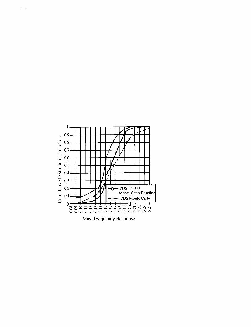
TheCDFresultsfor thePDSmethodsareplottedalongwith the 1000sampleMC

baselinesimulationin Figure4 andTable3. TheMC baselineCDF isextremely

unsymmetric,sothisclearlycausesaproblemfor thereliabilitymethods.Thisasymmetry

maybedueto thefactthatthemaximumresponseisobtainedbyscanningtheresponseof

differentnodes,andthismayskewthedistribution.Furtherexaminationof thisphenomena

wasperformedonamoredetailedbladed-disk,whichwill bereportedin thefuture,and

additionalwork isalsoneeded.It isalsonotedthatthereis fair agreementbetweentheMC

baselineresultandthatobtainedfrom MC usingdynamicrv's. Theerrorsfor thedesign

pointat .99arestill around10%for bothPDSmethods,though,which is within reason

especiallywhenoneconsidersthatatpresent,therearenoalternativemethodsfor obtaining

thismaximumvalue. Aswith thefree-responseanalysis,thesignificanterrorin the

standarddeviationandthelackof coincidenceof thecurvesindicatedvisuallysignifiesthat

thereis still errorpresentin themethods.An additional sourceof errorin thereliability

methodsfor thisanalysisis theextentto whichthemaximumrespondingdof doesnothave

asmoothdependenceon therv's. Possiblediscontinuitiesin thisdependencewouldcause

errorsin theresponsesurfacegenerationcreatedusingnumericaldifferentiation.An

examinationof theruntimesyieldssimilarresultsasthefreeresponsecase,with theMC

baselinetaking27.3hoursof wall-clocktime,thePDSMC taking18.5minuteswall-clock,

andthePDSFORM takingabout90seconds.Becauseof theacceptablelevel of error for

design,theincreasedaccuracyin systemvariabilityobtainedby usingdynamicratherthan

17

primitiverv's, andthetremendousreductionincomputertime,thetechniquewasappliedto

thesolutionof amistunedbladed-disk,whichwill bereportedin afuturepaper.

Conclusions

A probabilisticdynamicsynthesismethodhasbeenappliedto theanalysisof a

realisticthree-substructuresystem.Thenewtechniqueusesmodaldatafrom asampleset

of substructuresto generateasetof dynamicrandomvariableswhichfully describethe

probabilisticvariationin thestructures.Theresidualflexibility methodof componentmode

synthesisis thenusedto generateprobabilisticmassandstiffnessmatriceswhichcanbe

usedto obtainanydesiredresponsevariable.Probabilisticanalysisisperformedon these

stochasticsystemsby applyingboththetraditionalMonteCarlotechniqueandnew

reliabilitymethods.Solutionsfor bothfreeandforcedresponseof therealisticsystemwere

obtained,andtheresultscomparefavorablywith abaselineMonteCarloanalysis.Thenew

methodresultsin adramaticdecreaseincomputerrun-timeaswell asincreasedaccuracyin

representationof theprobabilisticvariationof theparametersof thestructuralsystem.

18

References

1 Brown, A.M. and Ferrri, A.A., "Probabilistic Component Mode Synthesis of

Nondeterministic Substructures," AIAA Jouirnal, Vol. 34, No.4, 1996, pp. 830-834.

2 Brown, A.M., "Development of a Probabilistic Dynamic Synthesis Method for the

Analysis of Non-Determinististic Structures," Ph.D. Dissertation, Georgia Institute of

Technology, 1998, pp. 18-51.

3 Cornell, C.A., "A Probability-Based Structural Code," Journal of the American

Concrete Institute, Vol. 66, No. 12, December 1969, pp. 974-985.

4 Hasofer, A.M. and Lind, N.C., "Exact and Invariant Second Moment Code

Format," Journal of the Engineering Mechanics Division, ASCE, Vol. 100, No. EM1,

1974, pp. 111-121.

5 Rackwitz, R., "Practical Probabilistic Approach to Design," Bulletin No. 112,

Comite Europen du Beton. Paris, France, 1976.

6 Rackwitz, R. and Fiessler, B., "Structural Reliability Under Combined Random

Load Sequences," Computer and Structures, Vol. 9, No. 5, 1978, pp. 489-494.

7 Chen, X. and Lind, N.C., "Fast Probability Integration by Three-Parameter Normal

Tail Approximation," Structural Safety, Vol. 1, 1983, pp. 269-276.

8 Wu, Y-T., and Wirsching, P., "New Algorithm for Structural Reliability

Estimation," Journal of Engineering Mechanics, ASCE, Vol. 113, No. 9, September, 1987,

pp. 1319-1336.

9 Wu, Y.T., "FPI Theoretical Manual, NESSUS Reference Manual," Southwest

Research Institute, Version 1.0, 1991.

10 MacNeal, R.H., "A Hybrid Method of Component Mode Synthesis," Computers

and Structures, Vol. 1, 1971, pp. 581-601.

11Craig, R.R. and Chang, C., "Free-Interface Methods of Substructure Coupling for

Dynamic Analysis," AIAA Journal, Vol. 14, No. 11, 1976, pp.1633-1635.

12Martinez, D.R., Came, T.G. and Miller, A.K., "Combined Experimental/Analytical

Modeling Using Component Mode Synthesis," Proceeding of the 25th Structures,

Structural Dynamics and Materials Conference, May 1984, pp. 140-152.

13Bookout, P., "Statistically Generated Weighted Curve Fit of Residual Functions

for Modal Analysis of Structures," NASA TM 108481, 1995.

14Craig, R., "Structural Dynamics; An Introduction to Computer Methods.," New

York: John Wiley and Sons, 1981.

19

15Admire,J.R.,Tinker,M.L. andIvey,E.W.,"ResidualFlexibilityTestMethodfor

Verificationof ConstrainedStructuralModels,"AIAA Journal, Vol. 32, No. 1, 1994, pp.

170-175.

16Ginsberg, J.H., and Pham, H., "Forced response of a continuous harmonic

system displaying eigenvalue veering phenomena," ASME Journal of Vibration and

Acoustics, Vol. 117, 1995, pp. 439-444.

17Wu, Y.T., "FPI Theoretical Manual, NESSUS Reference Manual," Southwest

Research Institute, Version 1.0, 1991, p. 37.

20

"Applicationof aProbabiliticDynamicSynthesisMethod...", A. M. Brown,Paper#J24252

FigureCaptionsPage

Fig. 1

Fig. 2

Fig. 3

Fig. 4

Jointprobabilitydensitysurface

3-Substructuresystem

3-Substructuremode3 naturalfrequencycomparingMonteCarlowith PDS

Percenterrorsfor forcedresponsesolution

g(u1,u2)=OUl

u2

1

0.9

0.8

0.7

0.6

0.5

0.4

0.3

0.2,

0.1,

0 ,

/.,¢Y

de,T

._'_ --I_:1.-- PD8 FORM [___t_ _t _ Monte Carlo BaslLr.'l II,llln,llsIIIIPDS Monte Carlc

Third natural frequency (hz)

/

r

Max. Frequency Response

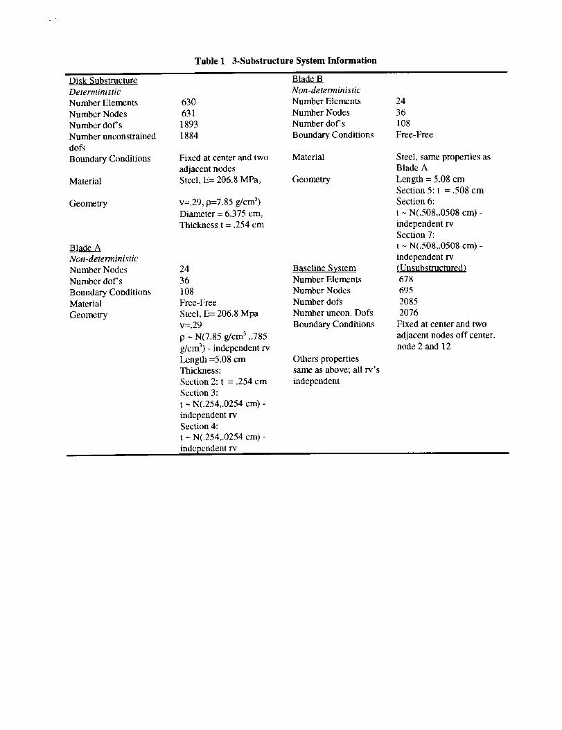
Table 1 3-Substructure System Information

Disk Subs_ctu_Deterministic

Number Elements

Number Nodes

Number dof's

Number unconstrained

dofs

Boundary Conditions

Material

Geometry

Blade?,Non-deterministic

Number Nodes

Number dof's

Boundary ConditionsMaterial

Geometry

630

631

1893

1884

Fixed at center and two

adjacent nodesSteel, E= 206.8 MPa,

v=.29, 9=7.85 g/cm 3)

Diameter = 6.375 cm,Thickness t = .254 cm

24

36108

Free-Free

Steel, E= 206.8 Mpav--.29

p ~ N(7.85 g/cm 3 ,.785

g/cm 3) - independent rv

Length =5.08 cmThickness:

Section 2: t = .254 cm

Section 3:

t ~ N(.254,.0254 cm) -

independent rvSection 4:

t - N(.254,.0254 cm) -

independent rv

Blade BNon-deterministic

Number Elements

Number Nodes

Number dof's

Boundary Conditions

Material

Geometry

Baseline SystemNumber Elements

Number Nodes

Number dofs

Number uncon. Dofs

Boundary Conditions

Others propertiessame as above; all rv's

independent

24

36

108

Free-Free

Steel, same properties asBlade A

Length = 5.08 cmSection 5: t = .508 cm

Section 6:

t ~ N(.508,.0508 cm) -

independent rvSection 7:

t ~ N(.508,.0508 cm) -

independent rv(Unsubstructured)

678

695

2085

2076

Fixed at center and two

adjacent nodes off center,node 2 and 12

Table 2 Percent Errors for Free ResponseSolution

Parameter PDS form (%)Median 0.18

Std. Dev. 28.91

.01CDF Value -1.3

.99 CDF Value 0.69

PDS Monte Carlo(%)

0.03

19.97

1.36

-1.79

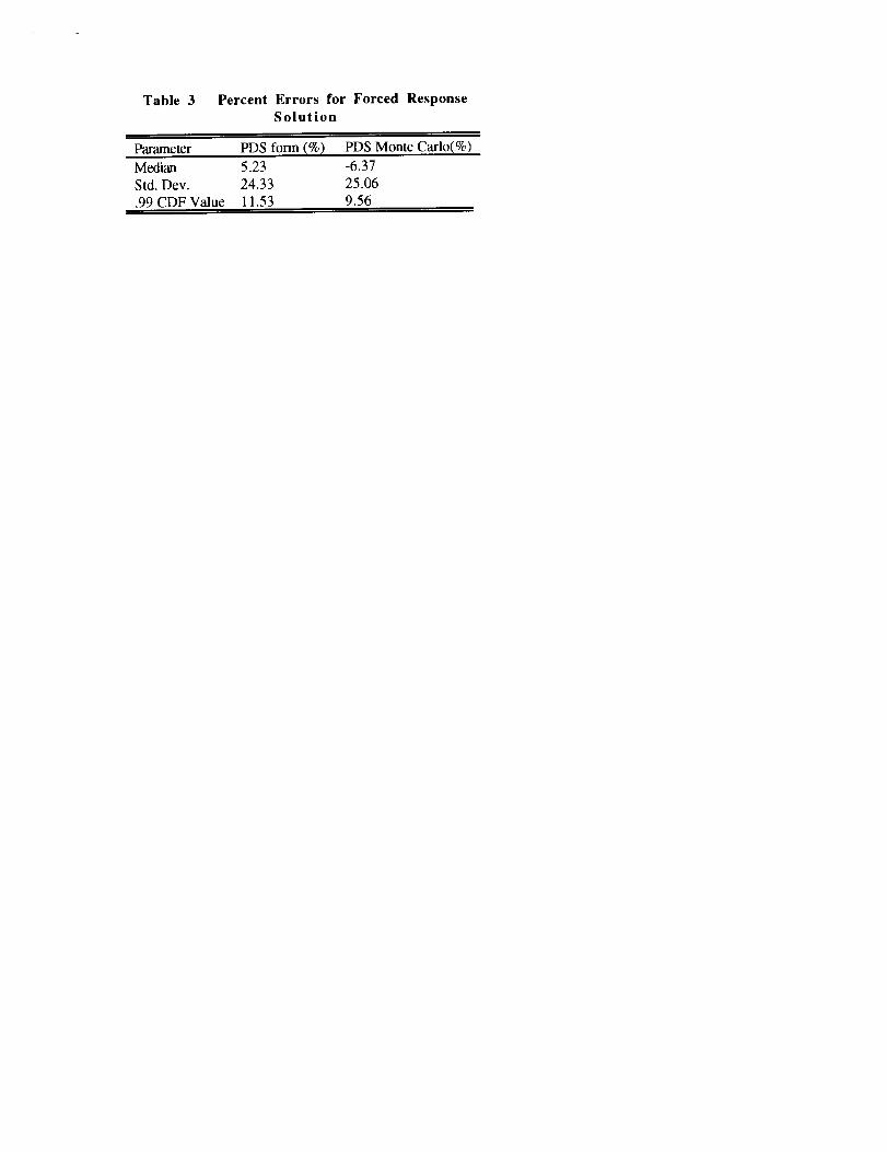
Table 3 Percent Errors for Forced ResponseSolution

Parameter PDS form (%)

Median 5.23

Std. Dev. 24.33

.99 CDF Value 11.53

PDS Monte Carlo(%)

-6.37

25.06

9.56