Discrete Dynamic Probabilistic Risk Assessment Model … · iii SAND2012-9346 Unlimited Release Printed October, 2012 Discrete Dynamic Probabilistic Risk Assessment Model Development

SANDIA REPORT SAND2012-9346 Unlimited Release Printed: October 2012

Discrete Dynamic Probabilistic Risk Assessment Model Development and Application

J. LaChance, J. Cardoni, Y. Li, A. Mosleh, D. Aird, D. Helton, K. Coyne

Prepared by Sandia National Laboratories Albuquerque, New Mexico 87185 and Livermore, California 94550

Sandia National Laboratories is a multi-program laboratory managed and operated by Sandia Corporation, a wholly owned subsidiary of Lockheed Martin Corporation, for the U.S. Department of Energy's National Nuclear Security Administration under contract DE-AC04-94AL85000.

Approved for public release; further dissemination unlimited.

ii

Issued by Sandia National Laboratories, operated for the United States Department of Energy

by Sandia Corporation.

NOTICE: This report was prepared as an account of work sponsored by an agency of the

United States Government. Neither the United States Government, nor any agency thereof,

nor any of their employees, nor any of their contractors, subcontractors, or their employees,

make any warranty, express or implied, or assume any legal liability or responsibility for the

accuracy, completeness, or usefulness of any information, apparatus, product, or process

disclosed, or represent that its use would not infringe privately owned rights. Reference herein

to any specific commercial product, process, or service by trade name, trademark,

manufacturer, or otherwise, does not necessarily constitute or imply its endorsement,

recommendation, or favoring by the United States Government, any agency thereof, or any of

their contractors or subcontractors. The views and opinions expressed herein do not

necessarily state or reflect those of the United States Government, any agency thereof, or any

of their contractors.

Printed in the United States of America. This report has been reproduced directly from the best

available copy.

Available to DOE and DOE contractors from

U.S. Department of Energy

Office of Scientific and Technical Information

P.O. Box 62

Oak Ridge, TN 37831

Telephone: (865) 576-8401

Facsimile: (865) 576-5728

E-Mail: [email protected]

Online ordering: http://www.osti.gov/bridge

Available to the public from

U.S. Department of Commerce

National Technical Information Service

5285 Port Royal Rd.

Springfield, VA 22161

Telephone: (800) 553-6847

Facsimile: (703) 605-6900

E-Mail: [email protected]

Online order: http://www.ntis.gov/help/ordermethods.asp?loc=7-4-0#online

mailto:[email protected]

http://www.osti.gov/bridge

mailto:[email protected]

http://www.ntis.gov/help/ordermethods.asp?loc=7-4-0#online

iii

SAND2012-9346 Unlimited Release

Printed October, 2012

Discrete Dynamic Probabilistic Risk

Assessment Model Development and

Application

Jeffrey LaChance and Jeffrey Cardoni

Sandia National Laboratories Albuquerque, NM 87185 USA

Yuandan Li, Ali Mosleh and David Aird

University of Maryland College Park MD

Donald Helton and Kevin Coyne

U.S. Nuclear Regulatory Commission Rockville, MD

ABSTRACT As part of an exploratory long-term research project, Sandia National Laboratories and the University of Maryland, under the support and guidance of the US Nuclear Regulatory Commission, developed a tool for conducting dynamic probabilistic risk analysis (PRA) for postulated severe accident scenarios by coupling and extending existing capabilities in hardware/phenomena and operator response simulation. The effort encompasses aspects of both Level 1 and Level 2 PRA. The dynamic PRA tool utilizes MELCOR as the code for simulating severe nuclear reactor accidents in a discrete dynamic event tree (DDET) framework. The Accident Dynamics Simulator (ADS) developed at the University of Maryland is used to generate the DDETs for an accident simulation that reflect variations in important parameters including: phenomenological events, the behavior of active and passive components, and operators’ cognitive activities and actions. Specific focus was placed on inclusion of an operator cognitive model in the dynamic PRA tool that addresses both pre-core damage human actions and post-core damage human actions. To that purpose, the Information, Decision, and Actions in a Crew (IDAC) context cognitive model developed at the University of Maryland was utilized. An existing ADS-IDAC model developed for a pressurized water reactor was expanded to address operator actions directed in both emergency operating procedures and severe accident management guidelines. The developed tool was applied to a demonstration problem; a station blackout (SBO) scenario at the Surry Nuclear Station. Both short-term and long-term SBO sequences were included in the demonstration evaluation. This report describes the developed tool and corresponding models and the results of the SBO demonstration problem. Insights from the demonstration evaluation, including potential further development of the dynamic PRA tool, are provided.

iv

ACKNOWLEDGEMENTS

The authors would like to acknowledge the following individuals:

Mark Leonard and Kenneth Wagner (dycoda, LLC) who provided guidance early in the project;

Tunc Aldemir, Richard Denning, Umit Catalyurek, and Kyle Metzroth (The Ohio State University) who were involved in the early planning of the project;

Martina Kloos (Gesellschaft für Anlagen und Reaktorsicherheit), Robert Lutz (Westinghouse Electric Company), Keith Woodard (ABS Consulting), and Enrico Zio (Ecole Centrale Paris and Supelec, Politecnico di Milano) who provided feedback on an intermediate project report; and

Charles Tinkler, Nathan Siu, James Chang, and Song-hua Shen (US Nuclear Regulatory Commission); Randall Gauntt, Doug Osborn, Noel Bellcourt, Don Kalinich, and John Reynolds (SNL); and Dongfeng Zhu (University of Maryland) who consulted throughout the project.

v

TABLE OF CONTENTS

ABSTRACT ..................................................................................................................... iii

ACKNOWLEDGEMENTS ...............................................................................................iv

LIST OF TABLES .......................................................................................................... viii

LIST OF FIGURES ..........................................................................................................ix

ACROYNMS ................................................................................................................. xiii

1. INTRODUCTION ...................................................................................................... 1

1.1 Background ........................................................................................................ 1

1.2 Objectives .......................................................................................................... 1

1.3 Scope and Limitations ........................................................................................ 3

1.4 Report Organization ........................................................................................... 4

2. DISCRETE DYNAMIC PRA METHODOLOGY ........................................................ 5

2.1 Existing Discrete Dynamic PRA Approaches ..................................................... 5 2.1.1 ADAPT/MELCOR ........................................................................................ 5

2.1.2 ADS/IDAC .................................................................................................... 7 2.1.3 MCDET ...................................................................................................... 10

2.2 Original Proposed Approach Description ......................................................... 11

2.3 Actual Tool Development ................................................................................. 13 2.3.1 ADS-IDAC—MELCOR (AIM) Coupling ...................................................... 16

2.4 Challenges Involved with the Internal Coupling of ADS-IDAC and MELCOR .. 23

2.4.1 MELCOR Errors in a Single Executable Application with ADS-IDAC ........ 23

2.4.2 MELCOR Performance Issues in AIM – Run-time Errors .......................... 24 2.4.3 Machine Dependency Issues for ADS-IDAC Input Files ............................ 25 2.4.4 Developing Procedural Input Files for ADS-IDAC and Format Error

Detection ................................................................................................... 25 2.4.5 AIM Bug with Time-delayed Operator Actions using Mental Beliefs .......... 26

3. DEMONSTRATION PROBLEM DESCRIPTION .................................................... 27

3.1 Selected Accident Scenario ............................................................................. 27

3.2 Assumptions and Boundary Conditions Used in Evaluation ............................. 28

3.3 Accident Response Procedures for a Station Blackout Scenario ..................... 29

3.4 Branching Parameters ..................................................................................... 32 3.4.1 TDAFW Pump Operation ........................................................................... 33 3.4.2 RCP Seal Leakage .................................................................................... 33

vi

3.4.3 Rate of Depressurization Using the SG PORVs (TDAFW Pump is Operating – LTSBO Only) ......................................................................... 35

3.4.4 Battery Duration/Depletion Time ................................................................ 36

3.4.5 Time When Power is Restored to Critical Instrumentation......................... 38 3.4.6 In-Vessel Accident Progression Phenomena ............................................. 39 3.4.7 Time to Initiation of Containment Spray Injection or ECST Refill Using Low-

Pressure Diesel-Driven Pump ................................................................... 45

4. DISCRETE DYNAMIC PRA TOOL DEVELOPMENT ............................................ 47

4.1 ADS-IDAC Model for Demonstration Problem.................................................. 47

4.1.1 Procedural Step/Calculation Aid Coding .................................................... 48

4.1.2 ADS Approach to Model Operators Following Parallel Procedures ........... 48 4.1.3 Operator Knowledge Base: Mental Belief .................................................. 49 4.1.4 ADS-IDAC Branching ................................................................................ 56 4.1.5 Crew Variation and Limited Indication Effect Captured in the Demonstration

Simulation ................................................................................................. 58

4.2 ADS Modifications ............................................................................................ 58

4.3 MELCOR Model for Demonstration Problem ................................................... 61 4.3.1 TDAFW Modeling for Long-Term Station Blackout Scenarios ................... 72

4.3.2 Godwin Pump Modeling for ECST Refill and Containment Sprays ............ 73 4.3.3 Simulating Operator Control of Steam Generator Cooldown Rate ............ 75 4.3.4 Estimating the Average Core Exit Thermocouple Temperature ................. 76

4.3.5 MELCOR Control Functions to Mimic Radiation Detector Response in Containment and Auxiliary Building ........................................................... 77

5. RESULTS OF DEMONSTRATION PROBLEM ...................................................... 83

5.1. Partial Results from AIM Demonstration Problem ............................................ 85

5.2. Run-time Considerations with the Demonstration Problem .............................. 86

5.3. AIM Results: Analysis and Demonstration of MELCOR and ADS-IDAC Interactivity ....................................................................................................... 87

5.3.1. MELCOR and ADS-IDAC Interactivity: TDAFW Throttling and DC power . 87 5.3.2. MELCOR and ADS-IDAC Interactivity: SG Cooldown Rate....................... 93

5.3.3 MELCOR and ADS-IDAC Interactivity: RCP Seal Leakage Rate .............. 93 5.3.4. Branch Parameter for DC Battery Life ....................................................... 96 5.3.5. Branch Parameter for Activation of Portable Generator ............................ 97 5.3.6 Branch Parameter for Timing of Godwin Pump Activation ......................... 97 5.3.7 Branching Order Performed by ADS-IDAC .............................................. 100

5.4. AIM Results: Overall Analysis of the Successfully Executed STSBO and LTSBO Simulations for Surry Demonstration Model ...................................... 102

5.4.1. Integral Hydrogen Generation ................................................................. 103 5.4.2. ECA0.0 to SAMG Procedure Transition: Core Exit Thermocouple

Temperature............................................................................................ 105

5.4.3. Environmental Release of Cesium-iodide ................................................ 111 5.4.4. Core Damage Progression ...................................................................... 117

vii

5.5 Operator Response Results ........................................................................... 120 5.5.1 Depressurize SGs to Cool Down the RCS............................................... 121 5.5.2 Use of Containment Sprays to Control Fission Product Release ............. 122

5.5.3 Control Flammability Condition of the Containment ................................. 123

6. SUMMARY AND RECOMMENDATIONS ............................................................ 127

6.1 Summary ........................................................................................................ 127

6.2 Potential Future Work .................................................................................... 128

7. REFERENCES..................................................................................................... 131

viii

LIST OF TABLES

Table 1. AIM Modifications to Existing MELCOR Subroutines. ......................................... 21

Table 2. TDAFW Pump Operation Branching Parameters. ............................................... 33 Table 3. WOG RCP Seal LOCA Model Parameters. .......................................................... 34

Table 4. RCP Seal LOCA Model Used in Demonstration Problem. ................................. 35

Table 5. RCS Cooldown Rate Branch Points. ...................................................................... 35 Table 6. Battery Depletion Branch Points. ............................................................................ 37

Table 7. Power Restoration to Instrumentation Branching Parameters. .......................... 39

Table 8. Time-at Temperature Model - Time Versus Temperature Relationship for Intact Fuel Rod Collapse. ......................................................................................... 40

Table 9. Radial Debris Relocation Time Distributions. ........................................................ 43 Table 10. Radial Debris Relocation Time Constants Used in Demonstration Problem. 43 Table 11. In-Vessel Accident Progression Branching Parameters. .................................. 45

Table 12. Containment Spray Initiation Branching Parameters. ....................................... 46

Table 13. Coded Procedures and Calculation Aids. ............................................................ 50

Table 14. Assumptions Used in Procedure Coding. ............................................................ 51

Table 15. Example Mental Belief in ADS-IDAC—Maintain Steam Generator Pressure. .................................................................................................................. 52

Table 16. Gaseous Effluent Monitor Classification Threshold. .......................................... 53

Table 17. Mental Beliefs Regarding Some Key Parameter Trends. ................................. 56

Table 18. Calculation Aid Curves Used in the Simulation. ................................................. 61

Table 19. Example: Use of a Calculation Aid in a Mental Belief. ...................................... 62

Table 20. MELCOR Plant Variables Sent to ADS-IDAC. ................................................... 64

Table 21. Important Plant Variables for ECA 0.0 and SAMG Procedures. ...................... 69

Table 22. Important Interactive Variables in the Surry MELCOR Model. ........................ 70

Table 23. COR Sensitivity Coefficients for Core Degradation Branches. ........................ 71

Table 24. TRIP Differences between RELAP5 and MELCOR. ......................................... 72 Table 25. Pressure vs. Time Functions for Different Cooldown Rates. ........................... 76

Table 26. SAMG Procedure Steps with Radiation Monitoring. .......................................... 78

Table 27. Automated AIM Branches for Demonstration Problem. .................................... 83

Table 28. Successful Automated AIM Branches for the Demonstration Problem. ......... 86 Table 29. Sequences for a STSBO, in Order of Branch According to ADS ID #. ......... 101

Table 30. Sequences for a STSBO, in Order of Execution Order ................................... 102 Table 31. Final Average Hydrogen Mass Generated by In-Vessel Reactions .............. 105 Table 32. Summary of Environment Release Fractions for CsI in AIM Simulations. ... 113

Table 33. Strategies/Equipment Unavailable in an SBO. ................................................. 121

ix

LIST OF FIGURES

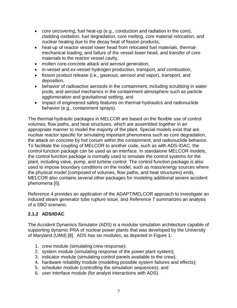
Figure 1. Architecture of the ADS dynamic PRA simulation program. ............................... 8

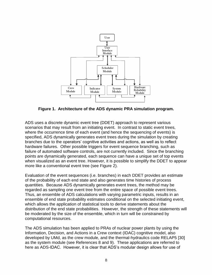
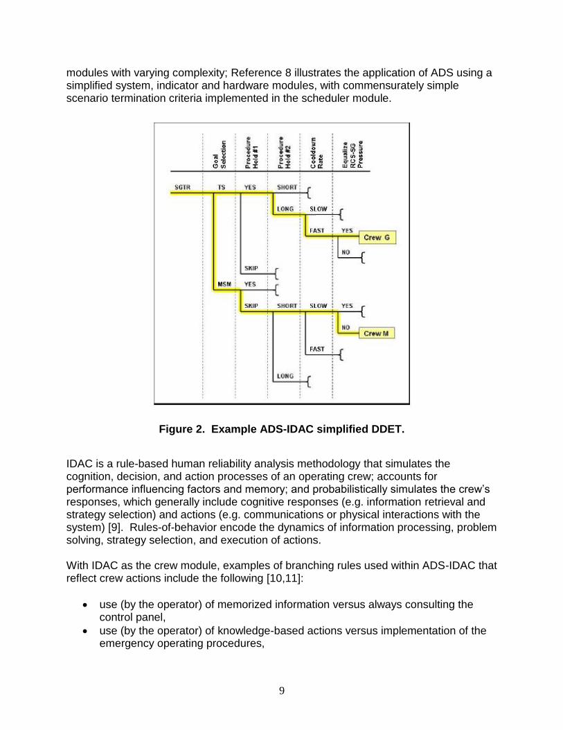
Figure 2. Example ADS-IDAC simplified DDET. .................................................................... 9 Figure 3. Proposed scheme for coupling ADAPT, ADS-IDAC, and MELCOR. ............... 13 Figure 4. Data interfaces in AIM. ............................................................................................ 17

Figure 5. Time-step control and AIM program flow. ............................................................ 18 Figure 6. AIM execution: code transitions between ADS-IDAC and MELCOR. ............. 19

Figure 7. EOP/SAMG station blackout overview ................................................................. 30 Figure 8. Battery depletion time cumulative probability distribution. ................................. 37

Figure 9. Zircaloy melt breakout temperature cumulative probability distribution. ......... 41 Figure 10. Molten clad drainage rate cumulative probability distribution. ........................ 42

Figure 11. Radial debis relocation time constants cumulative probability distributions (a) solidus and (b) liquidious. .............................................................................. 44

Figure 12. Input components of the Crew model ................................................................. 48 Figure 13. Possible procedural paths in the SBO scenarios. ............................................ 49

Figure 14. Calculation Aid-7, no venting, wet H2 measurement. ....................................... 59 Figure 15. Calculation Aid approximation in ADS. ............................................................... 60

Figure 16. SG-A nodalization and TDAFW modeling. ........................................................ 73 Figure 17. Godwin pump head curve. .................................................................................... 74

Figure 18. Containment nodalization and spray model. ..................................................... 75

Figure 19. Axisymmetric hydrodynamic mesh of the core and lower plenum ................. 77 Figure 20. Branches for Surry SBO demonstration calculation using AIM. ..................... 84

Figure 21. ADS-IDAC and MELCOR interactivity: TDAFW and DC power. .................... 88

Figure 22. TDAFW throttling for a LTSBO where DC battery depletion causes SG overfilling and TDAFWtrip. ................................................................................... 88

Figure 23. Primary and secondary pressure for LTSBO with TDAFW pump tripped due to SG overfilling. ............................................................................................ 89

Figure 24. Primary (RPV) and secondary (SG) water levels for LT-SBO with TDAFW tripped due to SG overfilling. ............................................................................... 89

Figure 25. TDAFW throttling for a LTSBO where DC depletion causes early loss of AFW......................................................................................................................... 90

Figure 26. Primary and secondary pressure for LTSBO where DC battery depletion causes early loss of the TDAFW pump. ............................................................ 91

Figure 27. Primary (RPV) and secondary (SG) water levels for LTSBO where DC battery depletion causes early loss of the TDAFW pump. ............................. 92

Figure 28. Comparison of core oxidation timing: effect of the TDAFW pump on accident progression (DC power ceases at 3.7 hours). .................................................. 92

Figure 29. AIM interactivity: operator control of SG cooldown rate for Surry LTSBO. ... 93

Figure 30. RCP seal leak rate and hydrogen generation for LTSBO simulations. ......... 94

Figure 31. RCP seal leak rate and containment pressure for LTSBO simulations – RCP leak rate does not greatly affect containment pressure. ....................... 95

Figure 32. RCP seal leak rate and hydrogen generation for STSBO simulations. ......... 95

Figure 33. RCP seal leak rate and containment water level below RPV in LTSBO simulations. ............................................................................................................ 96

Figure 34. Time of portable generator activation and hydrogen generation. .................. 97

Figure 35. Godwin pump used for ECST refill in LTSBO. .................................................. 98

x

Figure 36. Godwin pump used for containment sprays in LTSBO: effect on containment pressure. .......................................................................................... 99

Figure 37. Godwin pump used for containment sprays in LTSBO: effect on radiation ionization rate of containment atmosphere. ...................................................... 99

Figure 38. Godwin pump used for containment sprays in LTSBO: effect on hydrogen concentration and normalized water level in containment. ........................... 100

Figure 39. In-vessel hydrogen generation: LTSBO, best-estimate core degradation. . 103

Figure 40. In-vessel hydrogen generation: LTSBO, optimistic core degradation. ........ 104 Figure 41. In-vessel hydrogen generation: LTSBO, pessimistic core degradation. ..... 104

Figure 42. In-vessel hydrogen generation: STSBO, best-estimate core degradation. 106

Figure 43. In-vessel hydrogen generation: STSBO, optimistic core degradation. ........ 106 Figure 44. In-vessel hydrogen generation: STSBO, pessimistic core degradation. ..... 107

Figure 45. Core exit thermocouple temperatures: LTSBO, best-estimate core degradation. ......................................................................................................... 107

Figure 46. Core exit thermocouple temperatures: LTSBO, optimistic core degradation. ......................................................................................................... 108

Figure 47. Core exit thermocouple temperatures: LTSBO, pessimistic core degradation. ......................................................................................................... 108

Figure 48. Core exit thermocouple temperatures: STSBO, best-estimate core degradation. ......................................................................................................... 109

Figure 49. Core exit thermocouple temperatures: STSBO, optimistic core degradation. ......................................................................................................... 110

Figure 50. Core exit thermocouple temperatures: STSBO, pessimistic core degradation. ......................................................................................................... 110

Figure 51. CsI release fraction to environment: LTSBO, best-estimate core degradation. ......................................................................................................... 111

Figure 52. CsI release fraction to environment: LTSBO, optimistic core degradation. 112

Figure 53. CsI release fraction to environment: LTSBO, pessimistic core degradation. ......................................................................................................... 112

Figure 54. CsI release fraction to environment: STSBO, best-estimate core degradation. ......................................................................................................... 114

Figure 55. CsI release fraction to environment: STSBO, optimistic core degradation (scale is intentional to illustrate very low releases). ....................................... 114

Figure 56. CsI release fraction to environment: STSBO, pessimistic core degradation (scale is intentional to illustrate very low releases). ....................................... 115

Figure 57. Debris mass ejected after vessel breach for best-estimate LTSBO. ........... 116

Figure 58. Containment pressure for LTSBO with lower head failure at 15.8 hours and containment sprays at 17.3 hours. ................................................................... 116

Figure 59. Fuel damage progression: LTSBO, best-estimate core degradation. ......... 117 Figure 60. Fuel damage progression: LTSBO, optimistic core degradation. ................ 118

Figure 61. Fuel damage progression: LTSBO, pessimistic core degradation. .............. 118

Figure 62. Fuel damage progression: STSBO, best-estimate core degradation. ......... 119 Figure 63. Fuel damage progression: STSBO, optimistic core degradation. ................ 119

Figure 64. Fuel damage progression: STSBO, pessimistic core degradation. ............. 120 Figure 65. Operator action of controlling the SGs pressure ............................................. 122

Figure 66. Control of radioactive release from the containment...................................... 124

xi

Figure 67. Calculation Aid-7, no venting, wet H2 measurement ...................................... 124 Figure 68. Simulation data points of the containment condition in one AIM sequence 125

xii

xiii

ACROYNMS

ADAPT Analysis of Dynamic Accident Progression Trees ADS Accident Dynamics Simulator AFW Auxiliary Feedwater AIM ADS-IDAC/MELCOR APET Accident Progression Event Tree BWR Boiling Water Reactor CA Computational Aid CDF Cumulative Distribution Function CETC Core Exit Thermocouple CF Control Function C-SGTR Conditional Steam Generator Tube Rupture CST Condensate Storage Tank DDET Discrete Dynamic Event Tree DFC Diagnostic Flow Chart EAL Emergency Action Level ECMT Emergency Condensate Makeup Tank ECST Emergency Condensate Storage Tank EDMG Extensive Damage Mitigation Guidelines EOF Emergency Operation Facility EOP Emergency Operating Procedure GUI Graphical User Interface GRS Gesellschaft für Anlagen und Reaktorsicherheit IC Isolation Condenser IDAC Information, Decision, and Actions in a Crew context LFFG Large Fire, Flood Guideline LOCA Loss of Coolant Accident LOOP Loss of Offsite Power LTSBO Long Term Station Blackout MAAP Modular Accident Analysis Program MACCS MELCOR Accident Consequence Code System MCCI Molten Core-Concrete Interaction MCDET Monte Carlo Dynamic Event Tree MELCOR not an acronym OAT Action Taker Operator ODM Decision Maker Operator NRC US Nuclear Regulatory Commission OSU Ohio State University PORV Power-Operated Relief Valve PRA Probabilistic Risk Assessment PSA Probabilistic Safety Assessment PWR Pressurized Water Reactor RCIC Reactor Core Isolation Cooling RCP Reactor Coolant Pump RCS Reactor Coolant System

xiv

RPV Reactor Pressure Vessel SAG Severe Accident Guideline SAMG Severe Accident Management Guidelines SBO Station Blackout SCG Severe Challenge Guideline SCST Severe Challenge Status Tree SG Steam Generator SGTR Steam Generator Tube Rupture SNAP Symbolic Nuclear Analysis Package SNL Sandia National Laboratories SOARCA State-of-the Art Reactor Consequence Analysis SRV Safety Relief Valve TDAFW Turbine Driven Auxiliary Feedwater TSC Technical Support Center UMd University of Maryland WOG Westinghouse Owners Group

1

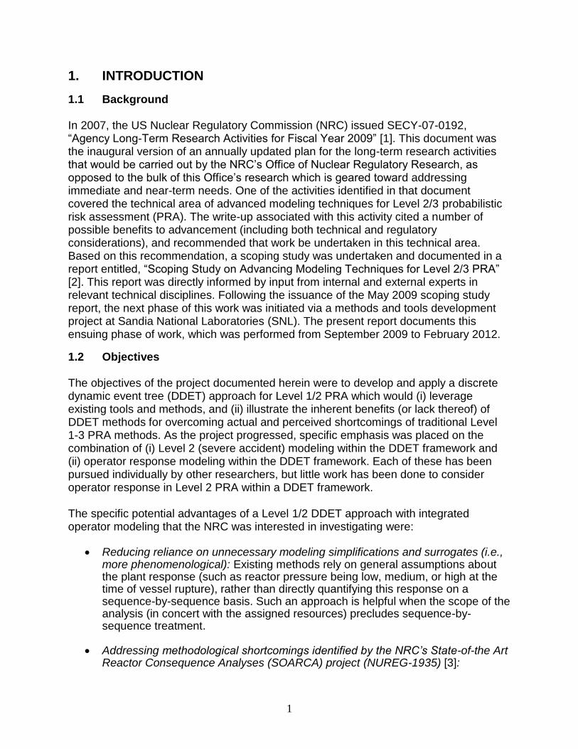
1. INTRODUCTION

1.1 Background In 2007, the US Nuclear Regulatory Commission (NRC) issued SECY-07-0192, “Agency Long-Term Research Activities for Fiscal Year 2009” [1]. This document was the inaugural version of an annually updated plan for the long-term research activities that would be carried out by the NRC’s Office of Nuclear Regulatory Research, as opposed to the bulk of this Office’s research which is geared toward addressing immediate and near-term needs. One of the activities identified in that document covered the technical area of advanced modeling techniques for Level 2/3 probabilistic risk assessment (PRA). The write-up associated with this activity cited a number of possible benefits to advancement (including both technical and regulatory considerations), and recommended that work be undertaken in this technical area. Based on this recommendation, a scoping study was undertaken and documented in a report entitled, “Scoping Study on Advancing Modeling Techniques for Level 2/3 PRA” [2]. This report was directly informed by input from internal and external experts in relevant technical disciplines. Following the issuance of the May 2009 scoping study report, the next phase of this work was initiated via a methods and tools development project at Sandia National Laboratories (SNL). The present report documents this ensuing phase of work, which was performed from September 2009 to February 2012.

1.2 Objectives The objectives of the project documented herein were to develop and apply a discrete dynamic event tree (DDET) approach for Level 1/2 PRA which would (i) leverage existing tools and methods, and (ii) illustrate the inherent benefits (or lack thereof) of DDET methods for overcoming actual and perceived shortcomings of traditional Level 1-3 PRA methods. As the project progressed, specific emphasis was placed on the combination of (i) Level 2 (severe accident) modeling within the DDET framework and (ii) operator response modeling within the DDET framework. Each of these has been pursued individually by other researchers, but little work has been done to consider operator response in Level 2 PRA within a DDET framework. The specific potential advantages of a Level 1/2 DDET approach with integrated operator modeling that the NRC was interested in investigating were:

Reducing reliance on unnecessary modeling simplifications and surrogates (i.e., more phenomenological): Existing methods rely on general assumptions about the plant response (such as reactor pressure being low, medium, or high at the time of vessel rupture), rather than directly quantifying this response on a sequence-by-sequence basis. Such an approach is helpful when the scope of the analysis (in concert with the assigned resources) precludes sequence-by-sequence treatment.

Addressing methodological shortcomings identified by the NRC’s State-of-the Art

Reactor Consequence Analyses (SOARCA) project (NUREG-1935) [3]:

2

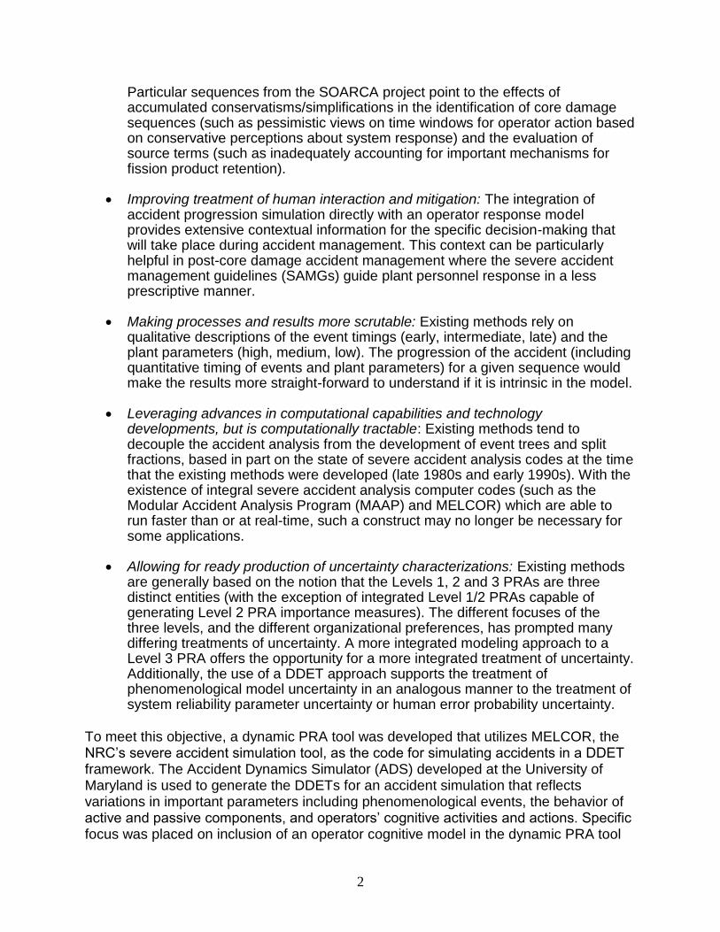
Particular sequences from the SOARCA project point to the effects of accumulated conservatisms/simplifications in the identification of core damage sequences (such as pessimistic views on time windows for operator action based on conservative perceptions about system response) and the evaluation of source terms (such as inadequately accounting for important mechanisms for fission product retention).

Improving treatment of human interaction and mitigation: The integration of

accident progression simulation directly with an operator response model provides extensive contextual information for the specific decision-making that will take place during accident management. This context can be particularly helpful in post-core damage accident management where the severe accident management guidelines (SAMGs) guide plant personnel response in a less prescriptive manner.

Making processes and results more scrutable: Existing methods rely on

qualitative descriptions of the event timings (early, intermediate, late) and the plant parameters (high, medium, low). The progression of the accident (including quantitative timing of events and plant parameters) for a given sequence would make the results more straight-forward to understand if it is intrinsic in the model.

Leveraging advances in computational capabilities and technology

developments, but is computationally tractable: Existing methods tend to decouple the accident analysis from the development of event trees and split fractions, based in part on the state of severe accident analysis codes at the time that the existing methods were developed (late 1980s and early 1990s). With the existence of integral severe accident analysis computer codes (such as the Modular Accident Analysis Program (MAAP) and MELCOR) which are able to run faster than or at real-time, such a construct may no longer be necessary for some applications.

Allowing for ready production of uncertainty characterizations: Existing methods

are generally based on the notion that the Levels 1, 2 and 3 PRAs are three distinct entities (with the exception of integrated Level 1/2 PRAs capable of generating Level 2 PRA importance measures). The different focuses of the three levels, and the different organizational preferences, has prompted many differing treatments of uncertainty. A more integrated modeling approach to a Level 3 PRA offers the opportunity for a more integrated treatment of uncertainty. Additionally, the use of a DDET approach supports the treatment of phenomenological model uncertainty in an analogous manner to the treatment of system reliability parameter uncertainty or human error probability uncertainty.

To meet this objective, a dynamic PRA tool was developed that utilizes MELCOR, the NRC’s severe accident simulation tool, as the code for simulating accidents in a DDET framework. The Accident Dynamics Simulator (ADS) developed at the University of Maryland is used to generate the DDETs for an accident simulation that reflects variations in important parameters including phenomenological events, the behavior of active and passive components, and operators’ cognitive activities and actions. Specific focus was placed on inclusion of an operator cognitive model in the dynamic PRA tool

3

that addresses both pre-core damage and post-core damage human actions. To that purpose, the Information, Decision, and Actions in a Crew (IDAC) context cognitive model developed at the University of Maryland was utilized.

1.3 Scope and Limitations This section describes the high-level scope and limitations associated with this project. More detailed descriptions related to the developed tool and a demonstration problem are provided later in the report. The scope of this project intentionally focuses on a subset of the overall risk profile that is substantively important to the overall risk (i.e., an accident class that is historically significant), that being station blackout (SBO) events. Furthermore, SBO sequences offer interesting aspects such as battery depletion and reactor coolant pump seal leakage which are component responses that have a strong effect on the accident progression. These types of situations, which are temporal in nature and do not represent the static/binary state transition that traditional methods are adept at handling, offer the most promise for the system/phenomenological aspects of DDET modeling. An SBO application is seen as fertile ground for DDET methods because it reduces the scope to something that is computationally manageable without trivializing the effort. In this study, the scope has been deliberately reduced to omit SBO-induced consequential steam generator tube rupture. This sub-set of SBO sequences offers its own complexities that a DDET approach might be well-suited to handle (e.g., the interplay between failure of different reactor coolant system (RCS) components and the system response), but also complicates the scope beyond what was prudent from a resource standpoint for a demonstration effort. Regarding the site selection, the Surry site was chosen as an expedient, and not due to any risk consideration. Due to work done for the SOARCA project, a contemporary Surry MELCOR input model was readily available, and plant response to station blackout events was well-characterized. In addition, past work for Level 1 PRA using ADS-IDAC had been performed for a plant very similar to Surry, though not for station blackout. Regarding the generality of the developed model, it is suited for the specific plant and the specific scenario utilized for its demonstration. The methods and approaches used are viewed to be applicable to any plant and any scenario. However, only Surry-specific design and operational information is included in the MELCOR input model, and only Surry SBO-specific emergency operating procedures (EOP) and SAMG procedures are included in the IDAC model. For ADS, only SBO-specific branching rules are included in the input model. It should be noted that Surry personnel did not participate in the generation or review of the implementation of the EOPs and SAMGs. All of the above reflect the demonstration nature of this project, and they serve to highlight the up-front “cost” of developing DDET simulation platforms.

4

Regarding the realism of the accident simulation results in this study, there are several key aspects to keep in mind. First, loss-of-offsite-power and failure of all emergency diesel generators is postulated at time zero. Such a condition has a low frequency of occurrence. Second, recovery of AC power via recovery of onsite equipment, use of auxiliary equipment, or implementation of offsite resources is not considered. This set of assumptions results in core damage being an inevitable outcome. Additional failures (e.g., turbine-driven auxiliary feedwater pump fails to start) and successes (e.g., backup generator used to power critical instrumentation) are modeled. However, only a subset of failures and successes are modeled, in line with the demonstration nature of this effort. Therefore, while efforts have been made to ensure that the results are reasonable for the sets of conditions that they represent, they are not intended to be best-estimate risk results for the Surry site or for this initiating event. Rather, it is the relative (not absolute) insights that are viewed as important. Due to technical issues that could not be resolved with the available resources, the evaluation of the demonstration problem was not completed. However, the evaluation did progress far enough to demonstrate the feasibility of modeling the dynamics of interactions between the plant and the operating crew actions with the AIM tool.

1.4 Report Organization The remainder of this report documents the work performed to develop and demonstrate the use of MELCOR coupled to ADS-IDAC. Section 2 provides background information on discrete dynamic PRA, including past development and its specific application in this study. Section 3 provides a description of the demonstration problem (a station blackout scenario at an operating pressurized-water reactor), including the scenario boundary conditions and branching assumptions. Section 4 describes the development of the tool itself, including the necessary code coupling, independent module modifications, and input model development. Section 5 provides the results of the demonstration problem in terms of the accident progression and operator action modeling, as well as the overall end-states. Finally, Section 6 provides the conclusions from this study, as well as illustrations of the types of insights that arise from a dynamic PRA treatment of a traditional reactor accident.

5

2. DISCRETE DYNAMIC PRA METHODOLOGY

The NRC in a white paper on advanced modeling techniques for Level 2/3 PRA [2] recommended development of a DDET method for advancing the Level 2/3 PRA methodology. This chapter provides an overview of some existing DDET methodologies. It also documents a proposed DDET tool that would utilize some of these existing tools and expand on them where necessary. Due to constraints, the proposed tool development effort was reduced in scope. The actual tool that was developed and the challenges that were experienced are documented in this section.

2.1 Existing Discrete Dynamic PRA Approaches Dynamic PRA methods were first developed over 25 years ago. A variety of tools and techniques have been proposed by many different organizations that have addressed the dynamic response of both plant systems and operators during an accident. A brief history of these methods is presented in Reference 4. Appendix B of Reference 2 discusses three recent discrete dynamic PRA approaches. The following sections provide descriptions of those three methods, acknowledging that other tools also exist, such as the Simulation Code System for Integrated Safety Assessment platform developed in Spain.

2.1.1 ADAPT/MELCOR

Analysis of Dynamic Accident Progression Trees (ADAPT) is a methodology for automated generation of accident progression event trees (APETs) that was developed by Ohio State University (OSU) and SNL [4,5] under a SNL lab-directed research project. ADAPT is intended to overcome the semi-static limitation associated with traditional approaches to constructing event trees (i.e., that top events in an APET or containment event tree loosely imply a sequence of events based on practitioner judgment and analysis of various accident progression scenarios). ADAPT is designed to work in tandem with a system simulator such as MELCOR that is capable of restarting calculations at specified points in time. In combination, ADAPT and the system simulator account for state changes in both active and passive systems to generate event trees. Branch points in the event tree can be generated due to:

behavior of active components (e.g., a valve failing on demand),

behavior of passive components (e.g., a steam generator tube spontaneously rupturing), or

phenomena (e.g., hydrogen combustion). For active components, the time of branch initiation is determined by the simulator based on user-supplied rules applied to process quantities computed by the system simulator (e.g., a predetermined percentiles along a predetermined distribution for valve failure probability) , rather than by sampling from a pre-determined distribution as is done in MCDET (Monte Carlo Dynamic Event Tree – see Section 2.1.3). For example, a demand may be placed on a valve to open or close when the computed pressure

6

exceeds a valve set point. Probabilities of the valve failure to open or close may be supplied. Crew actions are not simulated but may be represented to some extent by appropriate rules. User-defined rules are also used to specify failure criteria for passive components and the occurrence of phenomena as functions of process quantities. When branches occur, ADAPT pauses the system simulator and determines new branches to be computed and the restart conditions for each branch (i.e., one branch continues with original data, and another branch uses the new input data). The behavior of active and passive components and the occurrence of phenomena are regarded as aleatory uncertainties which result in the branches of each generated event tree. ADAPT allows for uncertainty in the user-defined criteria that define branch points and state transitions, and discretizes the cumulative distribution functions for the aleatory uncertain quantities in the branching criteria to determine the number of new branches and their associated probabilities. This means that rather than having a particular event (e.g., hydrogen deflagration) occur at a specified set of conditions, the user specifies a range of conditions and associated probabilities for which the event could occur. Reference 4 outlines an example where the time of creep rupture is determined from the pressure, temperature, and stress in the component, and where the threshold for rupture is also uncertain. The discretization approach used by ADAPT to determine new branches (rather than, for example, simple Monte Carlo sampling) ensures coverage of the range of uncertainty in state transitions. Other modeling characteristics (e.g., heat transfer coefficients) that are regarded as epistemic uncertainties are fixed throughout the generation of one event tree. Uncertainty in the epistemic quantities is propagated by generating multiple event trees, one for each set of values for code inputs. ADAPT is configured to generate multiple event trees in parallel. The generation of event trees within ADAPT is handled by a driver that manages branching rules (i.e., determines when a branch point is needed); handles system code initiation, termination, and file processing; determines scenario probabilities; and combines similar scenarios based on user criteria and system code results. Like other dynamic event tree approaches, ADAPT allows pruning of branches with probabilities below a user-specified threshold, and utilizes multi-processor capabilities to increase computational efficiency. MELCOR is a severe accident code developed by SNL for the NRC. Its primary purpose is to simulate the evolution of accidents in light water nuclear reactors and to generate fission product source terms. MELCOR is composed of several different physics modules, called packages (which are fully integrated), that model the following phenomena in severe nuclear accidents [6]:

thermal-hydraulics in the core, vessel, coolant system, cavity, containment, and auxiliary buildings,

7

core uncovering, fuel heat-up (e.g., conduction and radiation in the core), cladding oxidation, fuel degradation, core melting, core material relocation, and nuclear heating due to the decay heat of fission products,

heat-up of reactor vessel lower head from relocated fuel materials, thermal-mechanical loading, and failure of the vessel lower head, and transfer of core materials to the reactor vessel cavity,

molten core-concrete attack and aerosol generation,

in-vessel and ex-vessel hydrogen production, transport, and combustion,

fission product release (i.e., gaseous, aerosol and vapor), transport, and deposition,

behavior of radioactive aerosols in the containment, including scrubbing in water pools, and aerosol mechanics in the containment atmosphere such as particle agglomeration and gravitational settling, and

impact of engineered safety features on thermal-hydraulics and radionuclide behavior (e.g., containment sprays).

The thermal-hydraulic packages in MELCOR are based on the flexible use of control volumes, flow paths, and heat structures, which are assembled together in an appropriate manner to model the majority of the plant. Special models exist that are nuclear reactor specific for simulating important phenomena such as core degradation, the attack on concrete by hot corium within the containment, and radionuclide behavior. To facilitate the coupling of MELCOR to another code, such as with ADS-IDAC, the control function package can be used as an interface. In standalone MELCOR models, the control function package is normally used to simulate the control systems for the plant, including valve, pump, and turbine control. The control function package is also used to impose boundary conditions on the model, such as mass/energy sources where the physical model (composed of volumes, flow paths, and heat structures) ends. MELCOR also contains several other packages for modeling additional severe accident phenomena [6]. Reference 4 provides an application of the ADAPT/MELCOR approach to investigate an induced steam generator tube rupture issue, and Reference 7 summarizes an analysis of a SBO scenario.

2.1.2 ADS/IDAC The Accident Dynamics Simulator (ADS) is a modular simulation architecture capable of supporting dynamic PRA of nuclear power plants that was developed by the University of Maryland (UMd) [8]. ADS has six modules, as depicted in Figure 1:

1. crew module (simulating crew response); 2. system module (simulating response of the power plant system); 3. indicator module (simulating control panels available to the crew); 4. hardware reliability module (modeling possible system failures and effects); 5. scheduler module (controlling the simulation sequences); and 6. user interface module (for analyst interactions with ADS).

8

Figure 1. Architecture of the ADS dynamic PRA simulation program.

ADS uses a discrete dynamic event tree (DDET) approach to represent various scenarios that may result from an initiating event. In contrast to static event trees, where the occurrence time of each event (and hence the sequencing of events) is specified, ADS dynamically generates event trees during the simulation by creating branches due to the operators’ cognitive activities and actions, as well as to reflect hardware failures. Other possible triggers for event sequence branching, such as failure of automated software controls, are not currently included. Since the branching points are dynamically generated, each sequence can have a unique set of top events when visualized as an event tree. However, it is possible to simplify the DDET to appear more like a conventional event tree (see Figure 2). Evaluation of the event sequences (i.e. branches) in each DDET provides an estimate of the probability of each end state and also generates time histories of process quantities. Because ADS dynamically generates event trees, the method may be regarded as sampling one event tree from the entire space of possible event trees. Thus, an ensemble of ADS calculations with varying parametric inputs, results in an ensemble of end state probability estimates conditional on the selected initiating event, which allows the application of statistical tools to derive statements about the distribution of the end state probabilities. However, the strength of these statements will be moderated by the size of the ensemble, which in turn will be constrained by computational resources. The ADS simulation has been applied to PRAs of nuclear power plants by using the Information, Decision, and Actions in a Crew context (IDAC) cognitive model, also developed by UMd, as the crew module, and the thermal-hydraulics code RELAP5 [30] as the system module (see References 8 and 9). These applications are referred to here as ADS-IDAC. However, it is clear that ADS’s modular design allows for use of

9

modules with varying complexity; Reference 8 illustrates the application of ADS using a simplified system, indicator and hardware modules, with commensurately simple scenario termination criteria implemented in the scheduler module.

Figure 2. Example ADS-IDAC simplified DDET.

IDAC is a rule-based human reliability analysis methodology that simulates the cognition, decision, and action processes of an operating crew; accounts for performance influencing factors and memory; and probabilistically simulates the crew’s responses, which generally include cognitive responses (e.g. information retrieval and strategy selection) and actions (e.g. communications or physical interactions with the system) [9]. Rules-of-behavior encode the dynamics of information processing, problem solving, strategy selection, and execution of actions. With IDAC as the crew module, examples of branching rules used within ADS-IDAC that reflect crew actions include the following [10,11]:

use (by the operator) of memorized information versus always consulting the control panel,

use (by the operator) of knowledge-based actions versus implementation of the emergency operating procedures,

10

the activation of a mental belief (on the operator’s part) versus that mental belief remaining dormant,

the amount of time that a particular action takes, and inadvertent skipping of a procedure step.

2.1.3 MCDET The probabilistic dynamics method MCDET (Monte Carlo Dynamic Event Tree) [12,13] is a combination of Monte Carlo (MC) simulation and the DDET method. This method was developed at the Gesellschaft für Anlagen und Reaktorsicherheit (GRS; Germany) and has been implemented as a stochastic module which can operate together with a deterministic code (e.g., MELCOR; ATHLET) simulating the dynamics of the underlying system. The combination is capable of handling the interactions over time between stochastic processes simulated by MCDET and the system dynamics as modeled in the deterministic code. MCDET operates by randomly sampling an ensemble of event trees from the space of all event trees that follow from a selected initiating event [12]. In this sampling, the space of all event trees is defined by the underlying set of discrete and continuous random variables (usually aleatory) that describe the potential events (i.e., time of event and of system state changes due to the event). The Monte Carlo sampling is performed on these random variables. One element of this ensemble comprises a DDET. Evaluation of the DDET’s individual event sequences (i.e. branches) provides an estimate of the probability of each end state in the DDET conditional on the sampled values of the random variables. From the ensemble of event trees, the method obtains an ensemble of end state probability estimates conditional on the selected initiating event, which allows application of statistical tools to derive statements about the distribution of the end state probabilities. In its implementation, MCDET employs a scheduler to achieve efficiencies in calculation, such that event sequences are terminated if the sequence’s probability falls below a user-defined threshold and redundant computations for branches common to different sections of the tree are avoided [12]. MCDET is used in tandem with a deterministic system dynamics code that must be capable of restarting calculations at specified points in time. For each event sequence in a selected DDET in the ensemble, the combination of MCDET with the dynamics code also generates time histories of process quantities. Aggregation of these time histories over event sequences and over DDETs enables statistical statements about the distributions of these process quantities over time. An example application which teams MCDET with MELCOR 1.8.4 is discussed in Reference 12; another example application using ATHLET is presented in Reference 13. In addition, a Crew Module has been developed to couple with MCDET [14]. This module is able to simulate a procedure of operator actions as a dynamic process, including stochastic elements (e.g., the execution time of a particular action) and

11

deterministic elements (e.g., exchange of information through communications). This is accomplished through a set of user-prescribed lists (scripts) and program routines. However, the module does not attempt to model the mental process and cognitive behavior of the crew. In combination with MCDET, the Crew Module handles the time-dependent interactions between the human actions, system behavior, and stochastic events. MCDET results comprise estimates of end state probabilities and distributions of system state variables that conceptually result from integration over aleatory uncertainties (i.e. the sampled random variables) and are obtained numerically by Monte Carlo numerical integration methods. These estimates may themselves be uncertain due to epistemic uncertainty, and may be present in the definition of the probability models for the aleatory variables and in the characterization of inputs used by the system dynamics code. A straightforward method for assessing the epistemic uncertainty in these results would be to nest MCDET as the inner loop in a two-stage procedure, in which the outer loop indexes a sample from the probability space defined by epistemically uncertain quantities (an example of this approach is presented in Reference 13). However, in practice this method may be computationally demanding, as it requires evaluation of several ensembles of DDETs, one for each element in the sample from epistemically uncertain quantities. Reference 12 outlines a method for approximating the variance due to epistemic uncertainty in an output quantity by variance decomposition which requires computation for only two ensembles of DDETs.

2.2 Original Proposed Approach Description

As indicated in the previous sections, several DDET methods and tools are already available. The DDET approach proposed to the NRC was to leverage these tools to the extent possible. The recommended approach was to utilize the ADAPT/MELCOR tool with an interface to the ADS-IDAC model to provide a method for evaluating the dynamics of operator actions on an accident scenario. Merging of these tools would require consideration of the different features, operating systems, and limitations of the different software. Both ADAPT and ADS are used to dynamically generate event trees during an accident simulation in response to variations in important parameters including phenomenological events, the behavior of active and passive components, and operators’ cognitive activities and actions. Both programs, to different degrees, manage branching rules (i.e., determines when a branch point is needed); handles system code initiation, termination, and file processing; determines scenario probabilities; and combines similar scenarios based on user criteria and system code results. ADAPT has been used with MELCOR to simulate dynamic Level 2 PRA scenarios while ADS has been coupled with RELAP5 to simulate dynamic Level 1 PRA scenarios primarily in response to operator actions modeled using an IDAC model (referred to here after as an ADS-IDAC simulation). More detailed descriptions of these codes are provided in Reference 15.

12

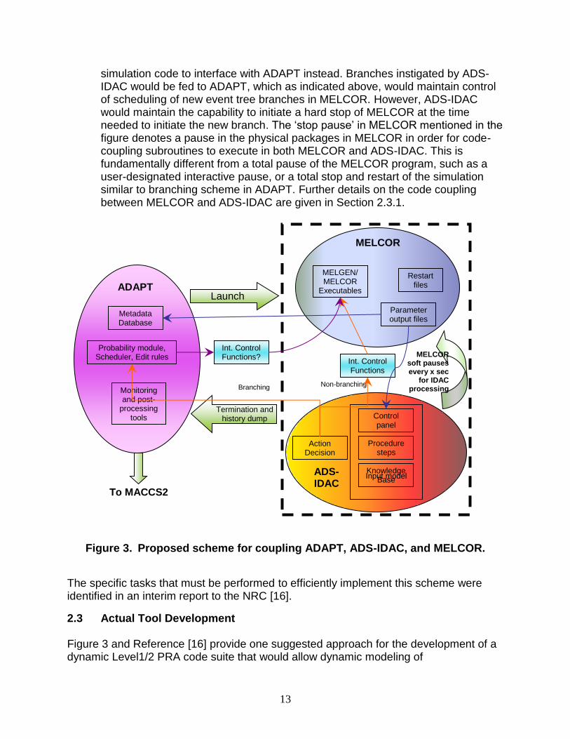
One important difference between the ADAPT/MELCOR and the ADS/RELAP5 branching logic involves how information is provided from the scheduler routines (i.e., ADAPT and ADS) to the simulation codes (i.e., MELCOR and RELAP5). The ADS logic uses input from the simulation code, processed through IDAC, to decide when branch on a new sequence based on an operator decision. The branching is accomplished through interactive control functions1 specified through an ADS-IDAC model to a RELAP5 input model. In the current ADAPT/MELCOR logic, control functions located within the MELCOR model stop the calculation at specified branching parameters. The reason for the stoppage is predetermined by the user and allows ADAPT to initiate a new MELCOR run to reflect the phenomenological event or component failure associated with the branching parameter that caused MELCOR to stop. Changing the ADAPT/MELCOR interface to look more like the ADS/RELAP5 interface is a possibility that was evaluated but not pursued at this time. A suggested approach for coupling of ADAPT, ADS-IDAC, and MELCOR is illustrated in Figure 3. The main points are summarized below:

1. Scheduling, process control, and sequence tracking would remain in ADAPT. All branching parameters and their values except for human actions would thus be input into ADAPT. The interface between ADAPT and MELCOR would be modified to utilize interactive control functions (i.e., some logic rules moved from MELCOR to ADAPT) as is done in the ADS framework. This approach would require that parameters from MELCOR that are used to make branching decisions be passed to ADAPT.

2. ADS-IDAC would communicate directly with MELCOR in order for MELCOR to feed the plant parameters needed by the IDAC model to make operator decisions. The provided parameter information would be provided at a defined interval (e.g., 0.5 s). Non-branching operator actions (e.g., controlling flow) would also be fed back from IDAC directives back to MELCOR through interactive control functions which is the current process used with the ADS-IDAC and RELAP5 interface.

3. Branching decisions based on operator actions would be passed directly from ADS-IDAC to ADAPT which would then schedule a new MELCOR branch. This would require redirecting the existing ADS-IDAC branching interface with the

1 Interactive control functions are used in reactor system models to set a condition to true or false or to a

specified value based on input from either an internal or external source. For example, interactive control functions can be used to simulate opening or closing a valve or adjusting the flow through a valve based on an operator decision generated from the IDAC code. Control functions are more powerful logic functions contained within a reactor system model that processes input information from one or more nodes in the model (or from other control functions) through a specified relational model that determines an output utilized in an accident simulation. In current applications of ADAPT-MELCOR, control functions are used to determine parameters (e.g., the Larsen-Miller correlation for creep rupture) that will stop the MELCOR evaluation when a specified value is obtained and allow ADAPT to initiate a new MELCOR evaluation with a dynamic modification to the accident scenario.

13

simulation code to interface with ADAPT instead. Branches instigated by ADS-IDAC would be fed to ADAPT, which as indicated above, would maintain control of scheduling of new event tree branches in MELCOR. However, ADS-IDAC would maintain the capability to initiate a hard stop of MELCOR at the time needed to initiate the new branch. The ‘stop pause’ in MELCOR mentioned in the figure denotes a pause in the physical packages in MELCOR in order for code-coupling subroutines to execute in both MELCOR and ADS-IDAC. This is fundamentally different from a total pause of the MELCOR program, such as a user-designated interactive pause, or a total stop and restart of the simulation similar to branching scheme in ADAPT. Further details on the code coupling between MELCOR and ADS-IDAC are given in Section 2.3.1.

Figure 3. Proposed scheme for coupling ADAPT, ADS-IDAC, and MELCOR.

The specific tasks that must be performed to efficiently implement this scheme were identified in an interim report to the NRC [16].

2.3 Actual Tool Development Figure 3 and Reference [16] provide one suggested approach for the development of a dynamic Level1/2 PRA code suite that would allow dynamic modeling of

ADS- IDAC

MELCOR

ADAPT

Int. Control Functions?

Parameter output files

Restart files

Input model

Procedure steps

Knowledge Base

Metadata Database

Probability module, Scheduler, Edit rules

Action Decision

Monitoring and post-

processing tools Control

panel

MELGEN/ MELCOR

Executables

To MACCS2

Int. Control Functions

Non-branching Branching

Launch

Termination and history dump

MELCOR soft pauses every x sec

for IDAC processing

14

phenomenological, component failure, and human actions. Additional efforts to include Level 3 aspects, in a seamless fashion, could also be performed. Unfortunately, because of resource limitations, the proposed DDET tool development plan discussed in Section 2.2 could not be fully exercised and the scope of the effort had to be reduced. The proposed plan was reviewed in order to identify what steps could be performed with available resources realizing that some modification to these steps may be required. Several objectives were used to help establish which steps should be pursued in the near term and which could be delayed. These objectives are:

1. The selected tasks should advance the development of one or more of the selected DDET tools (i.e., ADS-IDAC and ADAPT).

2. Tasks that will result in a more user friendly and efficient tool are of secondary importance for near-term efforts.

3. Code coupling issues (e.g., operating on a consistent platform) are important but are of secondary importance in the near-term.

4. Evaluation of the developed DDET tools is important but can be achieved through evaluation of a limited demonstration problem (i.e., a problem with fewer parameters selected for branching).

With these objectives in mind, the tasks outlined in Reference 16 were reviewed and two options were considered for proceeding with the available resources. Option A: The first option would be to utilize the existing ADAPT/MELCOR configuration for performing dynamic Level 2 analysis with no modifications except that the IDAC model would be incorporated into the ADAPT framework (i.e., a new task would involve encoding the IDAC logic into MELCOR control functions). Ohio State University has previously incorporated the SPAR-H human reliability model into the probabilistic branching rules in the ADAPT/MELCOR analysis of a SBO event [17]. To simulate operator performance during a severe accident, the IDAC knowledge base would have to be updated to reflect SAMG and Extensive Damage Mitigation Guidelines (EDMG) guidance. A sample problem evaluation would still be performed. Option B: The second option would be to use the ADS-IDAC simulation tool linked to MELCOR to perform a dynamic Level 2 analysis. The coupling of ADS-IDAC with MELCOR is a development that would be necessary for the development of the tool outlined in Section 2.2. ADS would perform the scheduling and branching for all the selected branching parameters including human errors (i.e., ADAPT would not be utilized in this option). As with the first option, the IDAC knowledge base would have to be updated to reflect SAMG and EDMG guidance. This option also removes the need to address code coupling issues since ADS-IDAC and MELCOR would be run on a Windows operating system. A sample problem evaluation would still be performed. In both options, tasks to improve the monitoring and post-processing capabilities of the desired DDET tool would be deferred to a possible future effort. In addition, since the ADS-IDAC and ADAPT programs would not be communicating in either option, tasks to

15

link the codes with both operating on same operating system also could be deferred to a possible future effort. Since both options require expanding the IDAC knowledge base into severe accident space, that effort should be pursued under the existing resources since it is an essential step forward in the DDET methodology and tool development outlined in Section 2.2. It was determined that the expansion of IDAC knowledge base could be accomplished within the available resources. Thus, the critical decision is whether to incorporate the IDAC logic into control function logic and utilize ADAPT as the dynamic simulator or to utilize ADS-IDAC as the dynamic simulator. In weighing these options it is important to recognize that ADAPT is a more powerful simulation tool in that it has been successfully utilized with multiple processors and has desirable post-processing features. The multi-processing capability of ADS-IDAC has only recently been improved and must be tested. As indicated above, the multi-processing and post-processing capabilities of the two codes are of secondary importance in this project. The incorporation of the IDAC logic into control functions is not viewed as a necessary step forward and actually would require additional effort that could not be accomplished with the available project resources. Based on these observations, Sandia recommended to the NRC to pursue Option B. The NRC concurred since Option B would advance the IDAC model into severe accident space, couple ADS-IDAC with MELCOR, and include a demonstration problem. All of these are necessary steps in the plan provided in Reference 16 The specific tasks from Reference 16 that were included in this study are listed below: ADS-IDAC Modifications

1. Modify an existing IDAC pressurized water reactor (PWR) pre-core damage operator response model, as necessary, to apply to the selected severe accident demonstration problem (a SBO at the Surry Nuclear Station - see Section 3 for more information). Identify which critical operator actions warrant branching and other operator actions that will not lead to branching but may interact with the MELCOR model through interactive control functions.

2. Modify the IDAC model to support SAMG implementation. The procedure-based portion of the model will be developed first followed by the development of the knowledge-based portion of the model. The Level 2 IDAC model modifications will be limited to the SAMGs pertinent for the demonstration problem.

3. Modify the IDAC model to support implementation of the 10 CFR 50.54 (hh)

actions (also referred to as the Extensive Damage Management Guidelines or EDMGs) that have been identified for the demonstration plant. This development will follow the incorporation of the SAMGs into the IDAC model.

16

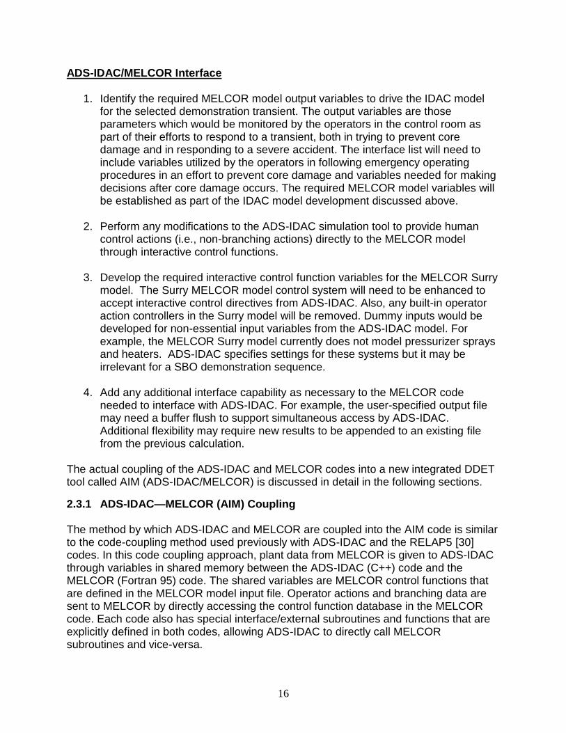
ADS-IDAC/MELCOR Interface

1. Identify the required MELCOR model output variables to drive the IDAC model for the selected demonstration transient. The output variables are those parameters which would be monitored by the operators in the control room as part of their efforts to respond to a transient, both in trying to prevent core damage and in responding to a severe accident. The interface list will need to include variables utilized by the operators in following emergency operating procedures in an effort to prevent core damage and variables needed for making decisions after core damage occurs. The required MELCOR model variables will be established as part of the IDAC model development discussed above.

2. Perform any modifications to the ADS-IDAC simulation tool to provide human

control actions (i.e., non-branching actions) directly to the MELCOR model through interactive control functions.

3. Develop the required interactive control function variables for the MELCOR Surry model. The Surry MELCOR model control system will need to be enhanced to accept interactive control directives from ADS-IDAC. Also, any built-in operator action controllers in the Surry model will be removed. Dummy inputs would be developed for non-essential input variables from the ADS-IDAC model. For example, the MELCOR Surry model currently does not model pressurizer sprays and heaters. ADS-IDAC specifies settings for these systems but it may be irrelevant for a SBO demonstration sequence.

4. Add any additional interface capability as necessary to the MELCOR code

needed to interface with ADS-IDAC. For example, the user-specified output file may need a buffer flush to support simultaneous access by ADS-IDAC. Additional flexibility may require new results to be appended to an existing file from the previous calculation.

The actual coupling of the ADS-IDAC and MELCOR codes into a new integrated DDET tool called AIM (ADS-IDAC/MELCOR) is discussed in detail in the following sections.

2.3.1 ADS-IDAC—MELCOR (AIM) Coupling The method by which ADS-IDAC and MELCOR are coupled into the AIM code is similar to the code-coupling method used previously with ADS-IDAC and the RELAP5 [30] codes. In this code coupling approach, plant data from MELCOR is given to ADS-IDAC through variables in shared memory between the ADS-IDAC (C++) code and the MELCOR (Fortran 95) code. The shared variables are MELCOR control functions that are defined in the MELCOR model input file. Operator actions and branching data are sent to MELCOR by directly accessing the control function database in the MELCOR code. Each code also has special interface/external subroutines and functions that are explicitly defined in both codes, allowing ADS-IDAC to directly call MELCOR subroutines and vice-versa.

17

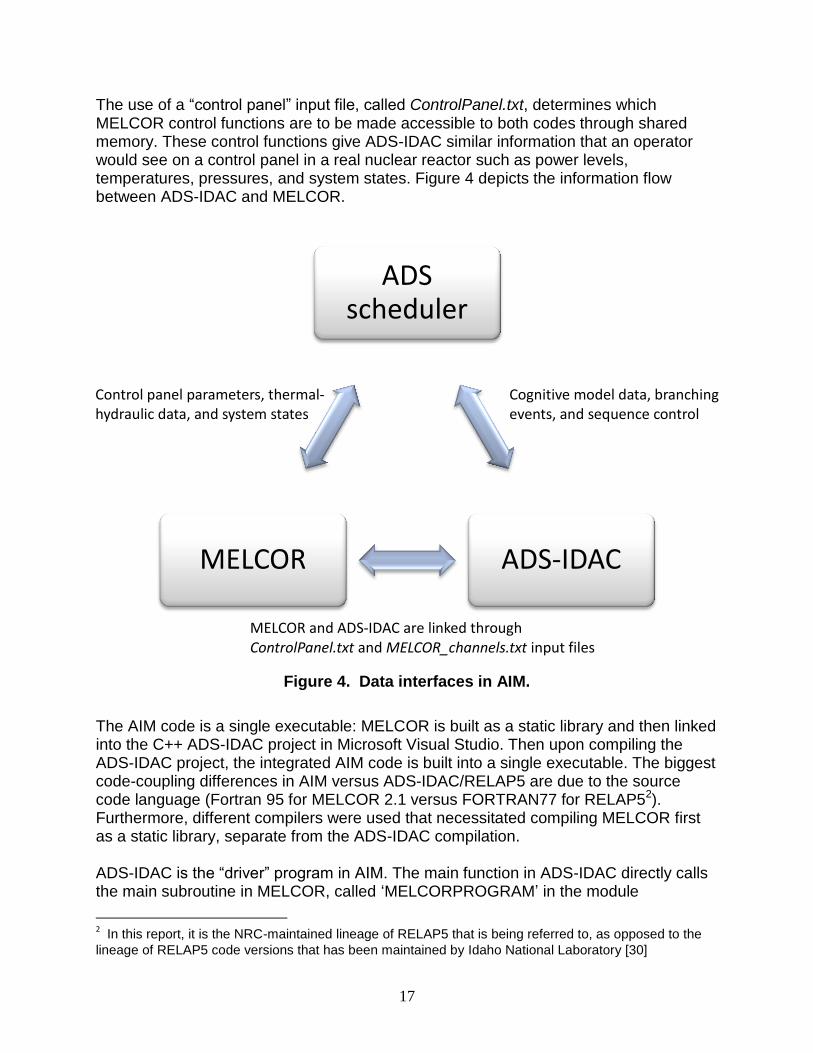
The use of a “control panel” input file, called ControlPanel.txt, determines which MELCOR control functions are to be made accessible to both codes through shared memory. These control functions give ADS-IDAC similar information that an operator would see on a control panel in a real nuclear reactor such as power levels, temperatures, pressures, and system states. Figure 4 depicts the information flow between ADS-IDAC and MELCOR.

Figure 4. Data interfaces in AIM.

The AIM code is a single executable: MELCOR is built as a static library and then linked into the C++ ADS-IDAC project in Microsoft Visual Studio. Then upon compiling the ADS-IDAC project, the integrated AIM code is built into a single executable. The biggest code-coupling differences in AIM versus ADS-IDAC/RELAP5 are due to the source code language (Fortran 95 for MELCOR 2.1 versus FORTRAN77 for RELAP52). Furthermore, different compilers were used that necessitated compiling MELCOR first as a static library, separate from the ADS-IDAC compilation. ADS-IDAC is the “driver” program in AIM. The main function in ADS-IDAC directly calls the main subroutine in MELCOR, called ‘MELCORPROGRAM’ in the module

2 In this report, it is the NRC-maintained lineage of RELAP5 that is being referred to, as opposed to the

lineage of RELAP5 code versions that has been maintained by Idaho National Laboratory [30]

ADS scheduler

ADS-IDAC MELCOR

Cognitive model data, branching events, and sequence control

Control panel parameters, thermal-hydraulic data, and system states

MELCOR and ADS-IDAC are linked through ControlPanel.txt and MELCOR_channels.txt input files

18

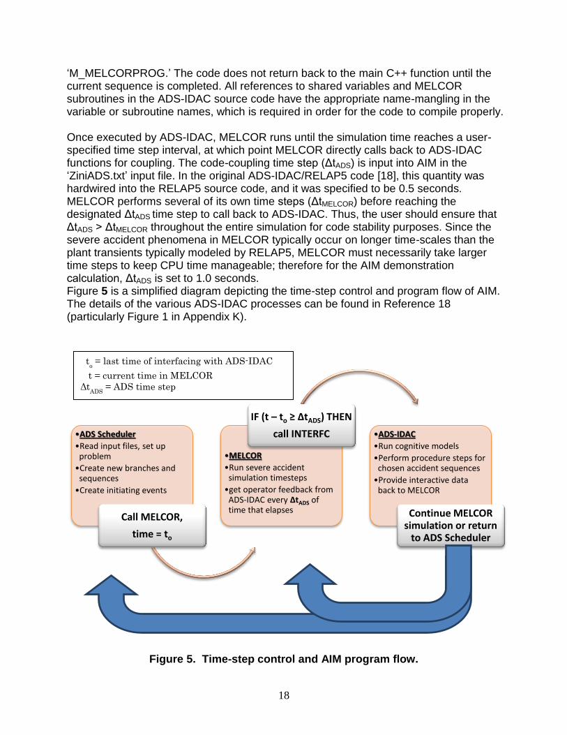
‘M_MELCORPROG.’ The code does not return back to the main C++ function until the current sequence is completed. All references to shared variables and MELCOR subroutines in the ADS-IDAC source code have the appropriate name-mangling in the variable or subroutine names, which is required in order for the code to compile properly. Once executed by ADS-IDAC, MELCOR runs until the simulation time reaches a user-specified time step interval, at which point MELCOR directly calls back to ADS-IDAC functions for coupling. The code-coupling time step (ΔtADS) is input into AIM in the ‘ZiniADS.txt’ input file. In the original ADS-IDAC/RELAP5 code [18], this quantity was hardwired into the RELAP5 source code, and it was specified to be 0.5 seconds. MELCOR performs several of its own time steps (ΔtMELCOR) before reaching the designated ΔtADS time step to call back to ADS-IDAC. Thus, the user should ensure that ΔtADS > ΔtMELCOR throughout the entire simulation for code stability purposes. Since the severe accident phenomena in MELCOR typically occur on longer time-scales than the plant transients typically modeled by RELAP5, MELCOR must necessarily take larger time steps to keep CPU time manageable; therefore for the AIM demonstration calculation, ΔtADS is set to 1.0 seconds. Figure 5 is a simplified diagram depicting the time-step control and program flow of AIM. The details of the various ADS-IDAC processes can be found in Reference 18 (particularly Figure 1 in Appendix K).

Figure 5. Time-step control and AIM program flow.

•ADS Scheduler

•Read input files, set up problem

•Create new branches and sequences

•Create initiating events

Call MELCOR,

time = to

•MELCOR

•Run severe accident simulation timesteps

•get operator feedback from ADS-IDAC every ΔtADS of time that elapses

IF (t – to ≥ ΔtADS) THEN

call INTERFC •ADS-IDAC

•Run cognitive models

•Perform procedure steps for chosen accident sequences

•Provide interactive data back to MELCOR

Continue MELCOR simulation or return

to ADS Scheduler

to = last time of interfacing with ADS-IDAC

t = current time in MELCOR

ΔtADS

= ADS time step

19

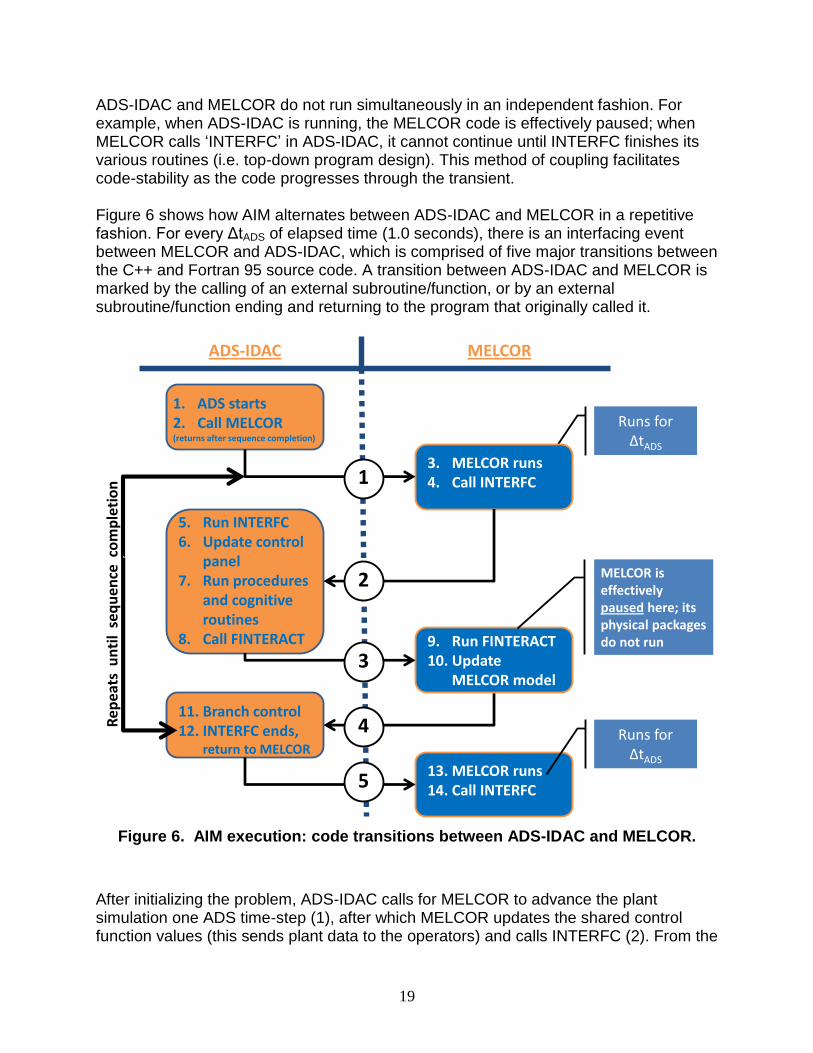
ADS-IDAC and MELCOR do not run simultaneously in an independent fashion. For example, when ADS-IDAC is running, the MELCOR code is effectively paused; when MELCOR calls ‘INTERFC’ in ADS-IDAC, it cannot continue until INTERFC finishes its various routines (i.e. top-down program design). This method of coupling facilitates code-stability as the code progresses through the transient. Figure 6 shows how AIM alternates between ADS-IDAC and MELCOR in a repetitive fashion. For every ΔtADS of elapsed time (1.0 seconds), there is an interfacing event between MELCOR and ADS-IDAC, which is comprised of five major transitions between the C++ and Fortran 95 source code. A transition between ADS-IDAC and MELCOR is marked by the calling of an external subroutine/function, or by an external subroutine/function ending and returning to the program that originally called it.

Figure 6. AIM execution: code transitions between ADS-IDAC and MELCOR.

After initializing the problem, ADS-IDAC calls for MELCOR to advance the plant simulation one ADS time-step (1), after which MELCOR updates the shared control function values (this sends plant data to the operators) and calls INTERFC (2). From the

ADS-IDAC MELCOR

13. MELCOR runs14. Call INTERFC

Runs for ΔtADS

Runs for ΔtADS

1. ADS starts 2. Call MELCOR (returns after sequence completion)

3. MELCOR runs4. Call INTERFC

5. Run INTERFC6. Update control

panel7. Run procedures

and cognitive routines

8. Call FINTERACT 9. Run FINTERACT10. Update

MELCOR model

11. Branch control12. INTERFC ends,

return to MELCOR

Re

pe

ats

un

til

seq

uen

ce c

om

ple

tio

n

MELCOR is effectively paused here; its physical packages do not run

1

2

3

4

5

20

INTERFC function, ADS-IDAC will read the updated control panel information from MELCOR, perform the appropriate plant procedures for the given accident sequence, run its cognitive operator functions, and return briefly to MELCOR by calling FINTERACT (3). In FINTERACT, the interactive control functions receive the operator action information from ADS-IDAC. Control function values are edited directly in the MELCOR database. At this point, however, the various physical packages in MELCOR do not execute further – MELCOR is still “paused” until ADS-IDAC finishes various branching functions in INTERFC (4). This may signal MELCOR to create a special restart for later execution of a different sequence. Finally, the INTERFC function finishes completely and MELCOR continues the transient for another ΔtADS time interval (5). Between each interface event MELCOR runs as it normally would in standalone MELCOR calculations. The version of MELCOR in the coupled AIM code is MELCOR 2.1 revision 4339, which was the latest revision of MELCOR 2.1 as of March 13, 2012.

2.3.1.1 MELCOR Source Code Additions – Building MELCOR Libraries for ADS-IDAC Coupling MELCOR with ADS-IDAC into an integral executable requires some modification to the Fortran 95 source code for MELCOR. MELCOR is compiled separately into static libraries using Intel Fortran Composer XE 2011 and MELCOR source assistant. These libraries are then linked with ADS-IDAC using Visual Studio 2010, and this process simultaneously compiles the C++ source code for ADS-IDAC. In order to facilitate future compilation of MELCOR for ADS-IDAC coupling, the source code additions in MELCOR were implemented into the SNL system for versioning and revision control for MELCOR, i.e. Apache Subversion (SVN). The additional Fortran subroutines for ADS-IDAC coupling, along with the limited direct modifications to existing MELCOR source code, are incorporated via ‘#IFDEF’ statements that are only seen by the compiler if “ADS” is defined as a compiler argument (i.e., /DADS). Therefore, compilation of standalone MELCOR executables is not affected by the AIM modifications and future MELCOR revisions are automatically incorporated into AIM. In order to compile optimized versions of the MELCOR static libraries, certain MELCOR subroutines should not be optimized; otherwise, the MELCOR code will not execute properly. For CPU intensive AIM calculations, comprised of dozens or hundreds of separate MELCOR simulations, it is essential to use optimized builds of MELCOR that execute significantly faster than un-optimized builds. Visual Studio 2010 alone cannot be used to properly build optimized MELCOR libraries. Visual Studio 2010 will optimize all or none of the MELCOR subroutines even though Intel Fortran Composer XE 2011 installs an add-on in the Visual Studio graphical user interface for compiling Fortran programs. Initial AIM calculations encountered ambiguous run-time errors when the MELCOR spray package (SPR) called subroutines that integrate systems of differential equations for MELCOR. Standalone MELCOR calculations, built using MELCOR Source Assistant did not exhibit the error under identical conditions. The final AIM calculations use

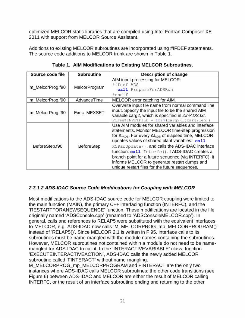
21

optimized MELCOR static libraries that are compiled using Intel Fortran Composer XE 2011 with support from MELCOR Source Assistant. Additions to existing MELCOR subroutines are incorporated using #IFDEF statements. The source code additions to MELCOR trunk are shown in Table 1.

Table 1. AIM Modifications to Existing MELCOR Subroutines.

Source code file Subroutine Description of change

m_MelcorProg.f90 MelcorProgram

AIM input processing for MELCOR: #ifdef ADS

call PrepareForADSRun

#endif

m_MelcorProg.f90 AdvanceTime MELCOR error catching for AIM.

m_MelcorProg.f90 Exec_MEXSET

Overwrite input file name from normal command line input. Specify the input file to be the shared AIM variable carg2, which is specified in ZiniADS.txt. Files%INPUTFILE = trim(carg2(1:carg2len))

BeforeStep.f90 BeforeStep

Use AIM modules for shared variables and interface statements. Monitor MELCOR time-step progression for ΔtADS. For every ΔtADS of elapsed time, MELCOR updates values of shared plant variables: call

R5ParUpdate(), and calls the ADS-IDAC interface

function: call Interfc().If ADS-IDAC creates a

branch point for a future sequence (via INTERFC), it informs MELCOR to generate restart dumps and unique restart files for the future sequences.

2.3.1.2 ADS-IDAC Source Code Modifications for Coupling with MELCOR Most modifications to the ADS-IDAC source code for MELCOR coupling were limited to the main function (MAIN), the primary C++ interfacing function (INTERFC), and the ‘RESTARTFORANEWSEQUENCE’ function. These modifications are located in the file originally named ‘ADSConsole.cpp’ (renamed to ‘ADSConsoleMELCOR.cpp’). In general, calls and references to RELAP5 were substituted with the equivalent interfaces to MELCOR, e.g. ADS-IDAC now calls ‘M_MELCORPROG_mp_MELCORPROGRAM()’ instead of ‘RELAP5()’. Since MELCOR 2.1 is written in F 95, interface calls to its subroutines must be name-mangled with the module names containing the subroutines. However, MELCOR subroutines not contained within a module do not need to be name-mangled for ADS-IDAC to call it. In the ‘INTERACTIVEVARIABLE’ class, function ‘EXECUTEINTERACTIVEACTION’, ADS-IDAC calls the newly added MELCOR subroutine called ‘FINTERACT’ without name-mangling. M_MELCORPROG_mp_MELCORPROGRAM and FINTERACT are the only two instances where ADS-IDAC calls MELCOR subroutines; the other code transitions (see Figure 6) between ADS-IDAC and MELCOR are either the result of MELCOR calling INTERFC, or the result of an interface subroutine ending and returning to the other

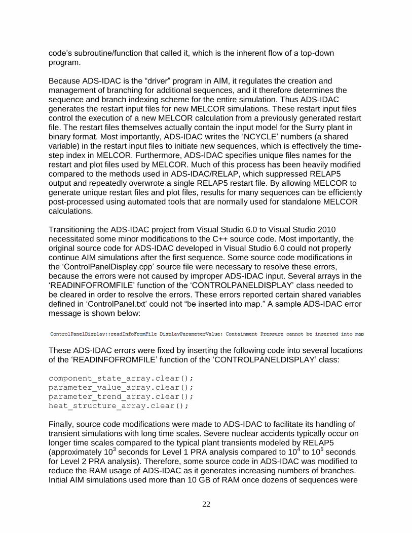
22

code’s subroutine/function that called it, which is the inherent flow of a top-down program. Because ADS-IDAC is the “driver” program in AIM, it regulates the creation and management of branching for additional sequences, and it therefore determines the sequence and branch indexing scheme for the entire simulation. Thus ADS-IDAC generates the restart input files for new MELCOR simulations. These restart input files control the execution of a new MELCOR calculation from a previously generated restart file. The restart files themselves actually contain the input model for the Surry plant in binary format. Most importantly, ADS-IDAC writes the ‘NCYCLE’ numbers (a shared variable) in the restart input files to initiate new sequences, which is effectively the time-step index in MELCOR. Furthermore, ADS-IDAC specifies unique files names for the restart and plot files used by MELCOR. Much of this process has been heavily modified compared to the methods used in ADS-IDAC/RELAP, which suppressed RELAP5 output and repeatedly overwrote a single RELAP5 restart file. By allowing MELCOR to generate unique restart files and plot files, results for many sequences can be efficiently post-processed using automated tools that are normally used for standalone MELCOR calculations. Transitioning the ADS-IDAC project from Visual Studio 6.0 to Visual Studio 2010 necessitated some minor modifications to the C++ source code. Most importantly, the original source code for ADS-IDAC developed in Visual Studio 6.0 could not properly continue AIM simulations after the first sequence. Some source code modifications in the ‘ControlPanelDisplay.cpp’ source file were necessary to resolve these errors, because the errors were not caused by improper ADS-IDAC input. Several arrays in the ‘READINFOFROMFILE’ function of the ‘CONTROLPANELDISPLAY’ class needed to be cleared in order to resolve the errors. These errors reported certain shared variables defined in ‘ControlPanel.txt’ could not “be inserted into map.” A sample ADS-IDAC error message is shown below:

These ADS-IDAC errors were fixed by inserting the following code into several locations of the ‘READINFOFROMFILE’ function of the ‘CONTROLPANELDISPLAY’ class: component_state_array.clear();

parameter_value_array.clear();

parameter_trend_array.clear();

heat_structure_array.clear();

Finally, source code modifications were made to ADS-IDAC to facilitate its handling of transient simulations with long time scales. Severe nuclear accidents typically occur on longer time scales compared to the typical plant transients modeled by RELAP5 (approximately 103 seconds for Level 1 PRA analysis compared to 104 to 105 seconds for Level 2 PRA analysis). Therefore, some source code in ADS-IDAC was modified to reduce the RAM usage of ADS-IDAC as it generates increasing numbers of branches. Initial AIM simulations used more than 10 GB of RAM once dozens of sequences were

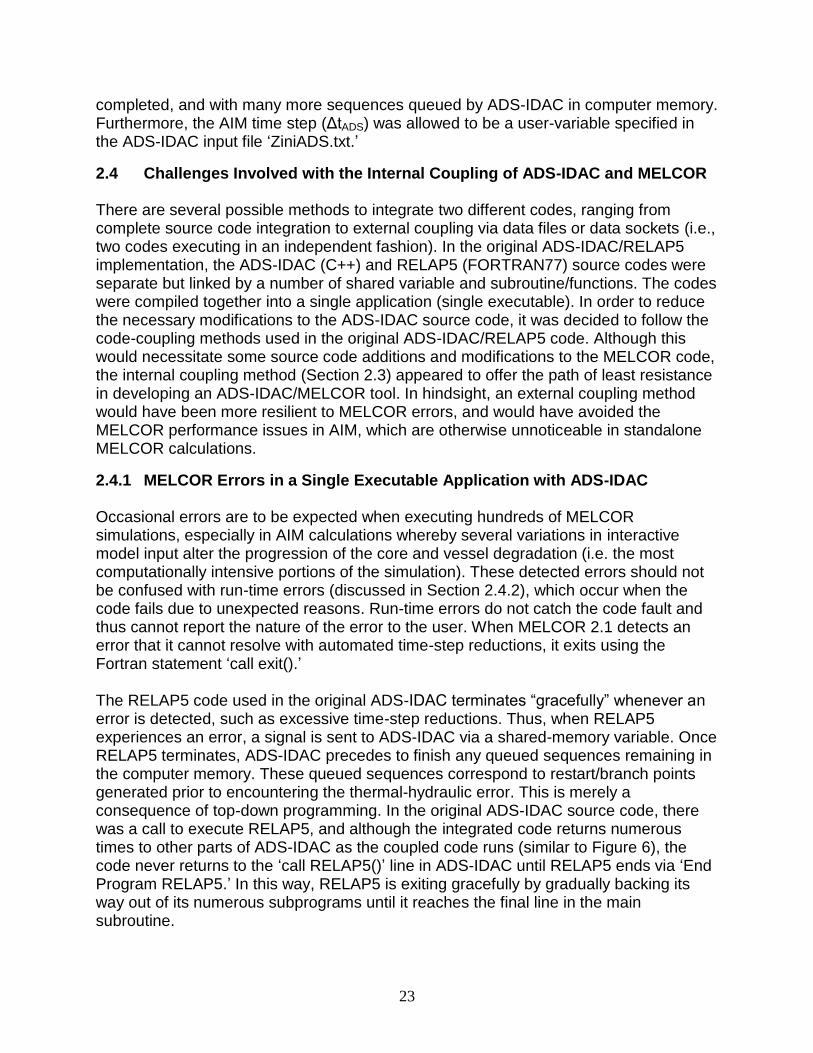
23

completed, and with many more sequences queued by ADS-IDAC in computer memory. Furthermore, the AIM time step (ΔtADS) was allowed to be a user-variable specified in the ADS-IDAC input file ‘ZiniADS.txt.’

2.4 Challenges Involved with the Internal Coupling of ADS-IDAC and MELCOR There are several possible methods to integrate two different codes, ranging from complete source code integration to external coupling via data files or data sockets (i.e., two codes executing in an independent fashion). In the original ADS-IDAC/RELAP5 implementation, the ADS-IDAC (C++) and RELAP5 (FORTRAN77) source codes were separate but linked by a number of shared variable and subroutine/functions. The codes were compiled together into a single application (single executable). In order to reduce the necessary modifications to the ADS-IDAC source code, it was decided to follow the code-coupling methods used in the original ADS-IDAC/RELAP5 code. Although this would necessitate some source code additions and modifications to the MELCOR code, the internal coupling method (Section 2.3) appeared to offer the path of least resistance in developing an ADS-IDAC/MELCOR tool. In hindsight, an external coupling method would have been more resilient to MELCOR errors, and would have avoided the MELCOR performance issues in AIM, which are otherwise unnoticeable in standalone MELCOR calculations.

2.4.1 MELCOR Errors in a Single Executable Application with ADS-IDAC Occasional errors are to be expected when executing hundreds of MELCOR simulations, especially in AIM calculations whereby several variations in interactive model input alter the progression of the core and vessel degradation (i.e. the most computationally intensive portions of the simulation). These detected errors should not be confused with run-time errors (discussed in Section 2.4.2), which occur when the code fails due to unexpected reasons. Run-time errors do not catch the code fault and thus cannot report the nature of the error to the user. When MELCOR 2.1 detects an error that it cannot resolve with automated time-step reductions, it exits using the Fortran statement ‘call exit().’ The RELAP5 code used in the original ADS-IDAC terminates “gracefully” whenever an error is detected, such as excessive time-step reductions. Thus, when RELAP5 experiences an error, a signal is sent to ADS-IDAC via a shared-memory variable. Once RELAP5 terminates, ADS-IDAC precedes to finish any queued sequences remaining in the computer memory. These queued sequences correspond to restart/branch points generated prior to encountering the thermal-hydraulic error. This is merely a consequence of top-down programming. In the original ADS-IDAC source code, there was a call to execute RELAP5, and although the integrated code returns numerous times to other parts of ADS-IDAC as the coupled code runs (similar to Figure 6), the code never returns to the ‘call RELAP5()’ line in ADS-IDAC until RELAP5 ends via ‘End Program RELAP5.’ In this way, RELAP5 is exiting gracefully by gradually backing its way out of its numerous subprograms until it reaches the final line in the main subroutine.

24

Unfortunately, MELCOR 2.1 does not terminate in such a fashion after experiencing an error. Instead, it ends via a ‘call exit()’ statement. In Fortran, ‘call exit()’ completely terminates the entire application. Thus the AIM code, which is a coupled application, will stop entirely if MELCOR experiences a fatal error, instead of recovering previously generated and queued sequences as it is designed to do. This issue is a consequence of: 1) the MELCOR source code, 2) the decision to couple the codes internally (if ADS-IDAC just called MELCOR like a script it would not be affected by any MELCOR errors), and 3) time limitations that only allowed for the development of the console version of ADS-IDAC and not the parallel version. The parallel version of ADS-IDAC is more resilient, but not completely immune, to errors in the thermal-hydraulic calculations, since a fatal error would only stop that particular calculation thread. Debugging MELCOR models in AIM is severely limited by the lack of any restart capability in the version of ADS-IDAC used in AIM. In complicated simulations of transient systems, occasional errors are often unavoidable. Such errors are mitigated by restarting the simulation from a recently generated restart point, which avoids having to rerun the entire simulation. At a restart point, various input parameters (e.g. time step size) are changed that allow the code to circumvent the error. This process is not practical with the version of ADS-IDAC used in AIM. Once an error is encountered, the entire calculation must be rerun from the very beginning–potentially costing weeks of CPU time. A restart capability in ADS-IDAC was recently developed after this work was completed.

2.4.2 MELCOR Performance Issues in AIM – Run-time Errors Since AIM is a coupled executable, MELCOR executes repetitively in a fashion that it normally would not–MELCOR never fully exits at the end of each MELCOR simulation as it would in standalone applications. Uninitialized variables, subroutine interface issues, and un-allocated memory are some potential issues that may never arise in standalone MELCOR, but they may cause MELCOR in AIM to behave inappropriately and experience run-time errors. Two particular code issues were encountered that significantly hindered the simulation of the Surry SBO demonstration problem with AIM. Both were resolved with code modifications:

1. Memory for the array ‘PlotData’ is allocated in ‘PlotInit.f90’ by calling ‘NewPlotDataAlloc.’ However, the memory is never de-allocated at the end of the MELCOR calculation. This causes MELCOR to fail by an "allocatable array is already allocated" run-time error if MELCOR is being run repeatedly by ADS-IDAC. This issue was resolved by adding a call to the subroutine ‘PlotDataDealloc,’ which de-allocates the memory set aside for the ‘PlotData’ array.

2. Despite proper optimization settings using MELCOR Source Assistant to compile MELCOR into static libraries, additional run-time errors were again encountered by the MELCOR SPR package. These errors occurred soon after the containment sprays were activated in the Surry SBO simulation and without any error message reported by the MELCOR code. Debugging revealed that the

25

code was inexplicably terminating in the ‘DERKF’ or ‘DERKFS’ subroutines, which use a Fehlberg Fourth-Fifth order Runge-Kutta method to integrate ordinary differential equations. This issue was resolved coincidentally by MELCOR 2.1 revisions 4292 and 4293. In these revisions, the SPR package variable ‘ZFALL’ was re-introduced as an argument for the subroutine ‘Drop_SPRDMZ.’ An earlier revision had removed the variable from the argument list for ‘Drop_SPRDMZ.’ The subroutines ‘Drop_SPRDMZ’ and ‘Drop_SPRDMT’ are both passed to the subroutine ‘DERKF’ (where the AIM calculations were failing) in an argument list, and Drop_SPRDMT contains ‘ZFALL’ as an argument. Drop_SPRDMZ and Drop_SPRDMT must have the same interface (i.e. argument list) when used in DERKF. Thus Drop_SPRDMZ must also contain ZFALL as an argument. Otherwise, run-time errors in the SPR package are encountered by MELCOR in its AIM implementation. MELCOR 2.1 revisions 4292 and 4293 involved modifications to the files ‘M_Drop.f90’ and ‘spryvl_NSI.f90.’

2.4.3 Machine Dependency Issues for ADS-IDAC Input Files The ADS-IDAC functions for input processing appear to have machine dependencies that can hide input format errors. For the operating system used to compile the AIM, the same operating system should be used to develop the ADS-IDAC input files; otherwise formatting errors may not be detected properly. For example, in this work AIM was compiled on a Windows 7 machine. During the development of the procedure input files for the Surry SBO sequences, text input files were created on a Windows XP machine and debugged on the Windows XP machine using the Windows 7 AIM executable. When the same input files were executed with AIM on the original Windows 7 machine used to build the code, several input formatting errors were encountered that were not detected by AIM on the Windows XP machine.

2.4.4 Developing Procedural Input Files for ADS-IDAC and Format Error Detection The version of ADS-IDAC used in AIM has very limited capabilities for detecting format errors in the operator procedure input files, thereby impeding the debugging of the more than 200 procedure input files for the demonstration problem. The procedure input files form the bulk of the input for ADS-IDAC and play a central role in determining the actions of the plant crew. Given limited user-friendly errors messages, developing and debugging these input files for new accident sequences is an extremely challenging and time-consuming process. For example, if ADS-IDAC detects an input format error it will report an error, but it will not give the input file or the input record that contains the error. A sample error message for a format error in a procedure input file is shown below: ProcedureStepUnit::readinfoFromFileNonResponseExit obj_type:691176823 cannot be

recognized

Given the above error message, the current strategy for debugging input format errors in the procedure files resorts to the following iterative guess-and-check process:

26

1. Remove all new procedure input files from the ‘Procedures.txt’ input file where all of the procedures for the simulation are defined.

2. Rerun AIM to confirm that the ADS-IDAC error message does not appear. 3. Incrementally add procedure steps to the ‘Procedures.txt’ file until the ADS-IDAC

error message occurs again. 4. Identify the procedure input file containing the improper input format. 5. Identify the culprit input record in the procedure input file that caused the error.

This may involve a guess-and-check process in and of itself. 6. Repeats steps 1-5 until all procedure input errors are resolved.

The 218 procedure input files for the Surry SBO AIM calculations required several months of development and debugging due to the limited input-error detection capabilities in ADS-IDAC.

2.4.5 AIM Bug with Time-delayed Operator Actions using Mental Beliefs In addition to the MELCOR ‘call exit()’ issue discussed in Section 2.4.1, AIM currently has an issue with handling time-delayed branching using mental beliefs in ADS-IDAC. This is exclusively an AIM issue since the ADS-IDAC/RELAP5 version generates time branches without any problem. This issue was first encountered when ADS-IDAC input files specified a 300 second time-delay for operator action in refilling the emergency condensate storage tank (ECST) via the Godwin pump, yet ADS-IDAC continually set the operator action delay to 20 seconds. A workaround was eventually developed using a fake procedural step to delay the operator action by 300 seconds. The time-delay issue was again discovered in the demonstration problem’s treatment of the Godwin pump branch. For the Surry SBO demonstration calculation, ADS-IDAC is supposed to vary the time to start the Godwin pump by one, two, and three hours after the operators make the decision to do so; this generates three branches in the process. The Godwin pump timing branches were implemented using mental beliefs. Unfortunately, the Godwin pump branch suffers from the ADS-IDAC bug with time-delayed mental beliefs. ADS-IDAC does not appropriately generate the three unique Godwin pump branches for the Surry SBO problem. Three branches are created but each activates the Godwin pump immediately after the decision is made by the operators to use the pump for either containment sprays or ECST refill. For a given Godwin branch point, all three Godwin branches will activate the pump at the same time. Consequently, the effective number of unique sequences simulated by AIM is essentially reduced by a factor of three in the demonstration problem.

Efforts to try and identify the source of this problem remain unsolved due to resource and time limitations.

27

3. DEMONSTRATION PROBLEM DESCRIPTION

3.1 Selected Accident Scenario

The selected demonstration problem can affect the amount of work required to develop and merge the necessary tools. For that reason, it is desirable to identify a demonstration problem that would help limit the amount of work necessary to provide validation of the tools and utility of the methodology. Four candidate demonstration scenarios were considered; three for a Westinghouse PWR (Surry) and one for a boiling water reactor (Peach Bottom). The demonstration scenarios and some important pros and cons for each are identified below: 1. Surry Station Blackout (SBO)

a) Pros: i) The most risk-significant sequence based on contemporary PRAs ii) Contains interesting modeling aspects including reactor coolant pump (RCP)

seal loss-of-coolant accident (LOCA) model, battery depletion, safety relief valve (SRV) sticking, power recovery, and treatment of turbine-driven auxiliary feedwater (TDAFW) after battery depletion

b) Cons: i) Treatment of actions in security-related procedures will create information

sensitivity issues ii) Insufficient information will exist for treatment of realistic RCP seal LOCA

model

2. Surry SBO with consequential steam generator tube rupture (C-SGTR) a) Pros:

i) May provide additional information to support ongoing NRC work in this area ii) Existing IDAC and ADAPT infrastructure is best suited to this problem

b) Cons: i) Lack of availability of steam generator (SG) flaw distribution information ii) Timing concurrent with other ongoing work could create complexities

3. Surry Interfacing System LOCA

a) Pros: i) Will contain the greatest number of potential human actions ii) Most closely related to an existing IDAC model

b) Cons: i) Slowest running MELCOR model ii) Little in the way of interesting phenomena suitable for branching

4. Peach Bottom SBO

a) Pros: i) The issue of effectiveness of reactor core isolation cooling (RCIC)

blackstart/blackrun(i.e., operation without DC control power) is an important issue

28

ii) Supporting information will be available from the SOARCA uncertainty analysis of the Peach Bottom long-term SBO

b) Cons: i) Treatment of actions in security-related procedures will create information

sensitivity issues ii) University of Maryland IDAC modelers have the least familiarity with this

scenario A decision was made for selecting a Surry SBO sequence without consequential SGTR as the demonstration problem. The rationale for selection of this scenario are:

Most risk-significant from a contemporary core damage frequency perspective

Preferred from a supporting information availability standpoint, relative to the other candidates (e.g., availability of flaw distributions for C-SGTR)

Allows investigation of TDAFW extension after battery depletion and effects of assumptions regarding RCP seal LOCA modeling

Well-suited given the PWR-centric nature of ADS-IDAC work to date

Existing baseline using traditional PRA methods

Better suited than some alternatives from a MELCOR run-time perspective

3.2 Assumptions and Boundary Conditions Used in Evaluation Key assumptions utilized in the demonstration problem include:

1. The SBO event is caused by a severe weather event that causes a loss-of-offsite power (LOOP). The diesel generators fail immediately resulting in a station blackout. The DC buses, batteries, and vital AC instrument buses are not damaged by the initiating event and are available to provide essential loads if power is restored. The severity of the damage is sufficient to prevent recovery of off-site power and recovery of the diesel generators (DGs) does not occur in the simulated time. The frequency of the combined severe weather-induced LOOP and random failure of the DGs is 1.2x10-6/yr [19].

2. The TDAFW pump train and the emergency condensate storage tank (ECST) are undamaged by the severe weather event and the TDAFW pump train automatically starts on low SG level. However, the potential for random failure and unavailability of the TDAFW pump is considered. The unavailability of the TDAFW pump (1.2 x10-2 per event) is dominated by the pump failing to start (7.0x10-3 per event) and being unavailable due to test and maintenance (5.0x10-3 per event). No recovery of the TDAFW pump is assumed to occur [19].

3. If the TDAFW pump initially operates, it operates until either the ECST depletes or after battery depletion occurs (failure of the TDAFW pump to run was not modeled). Upon battery depletion, the TDAFW pump will continue to run as long as water is available in the ECST. The valves controlling flow into the SGs from TDAFW will fail as-is and the TDAFW system will continue to operate until either:

29

(i) the SGs overfill and flood the steam lines which fails the pump turbine, or (ii) the SGs under fill causing a loss of sufficient steam to drive the TDAFW pump. Once flow from the TDAFW pump is lost, recovery of the pump will not be considered.

4. The steam generator power-operated relief valves (PORVs) are available for a manual cooldown of the primary system at a cooldown rate of less than 100 oF/hr, if TDAFW is available. Portable air cylinders (instrument air is lost during the SBO) and battery power are initially available for PORV operation. The SG PORVs close upon battery depletion and it is assumed the operators do not try to manually restore the valves to open position (e.g., by jacking the valve open or by connecting a portable battery to the valve).

5. Nominal RCP seal leakage (21 gpm per pump) occurs immediately after the SBO initiation due to loss of pump seal injection and cooling. Increased leakage may occur when the primary coolant fluid saturates within the RCP seal volume.

6. No coolant injection into the reactor coolant system (RCS) is available during a SBO to makeup inventory lost from the RCP seal leakage. Thus, core uncovery will eventually occur and the timing will be dependent upon the RCP seal leakage rate.

7. Connection of a portable, low-pressure (Godwin) diesel-driven pump is possible to provide makeup to the ECST (110,000 gallon capacity) or flow to the containment spray system. The water in the two firewater storage tanks (500,000 gallons total) is available for injection [20].

8. Upon battery depletion, all instrumentation will be unavailable. A portable power supply is available for restoring power to a vital AC bus in order to power all instrumentation required to exercise the procedures and guidelines for dealing with an SBO.

9. The containment is successfully isolated.

10. The Technical Support Center (TSC) is manned and operational one hour after the initiation of the SBO. The offsite Emergency Operations Facility (EOF) is manned at 1.5 hours after the initiation of the SBO. The TSC staff at one hour would begin consulting the appropriate SAMGs and EDMGs to provide guidance on alternative mitigation measures.

3.3 Accident Response Procedures for a Station Blackout Scenario Figure 7 provides an overview of the Emergency Operating Procedure (EOP) and Severe Accident Management Guidelines (SAMG) for the SBO scenario evaluated as

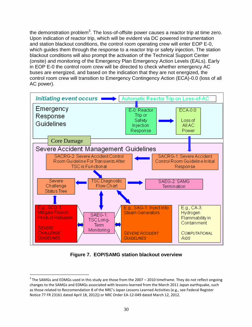
30

the demonstration problem3. The loss-of-offsite power causes a reactor trip at time zero. Upon indication of reactor trip, which will be evident via DC powered instrumentation and station blackout conditions, the control room operating crew will enter EOP E-0, which guides them through the response to a reactor trip or safety injection. The station blackout conditions will also prompt the activation of the Technical Support Center (onsite) and monitoring of the Emergency Plan Emergency Action Levels (EALs). Early in EOP E-0 the control room crew will be directed to check whether emergency AC buses are energized, and based on the indication that they are not energized, the control room crew will transition to Emergency Contingency Action (ECA)-0.0 (loss of all AC power).

Figure 7. EOP/SAMG station blackout overview

3 The SAMGs and EDMGs used in this study are those from the 2007 – 2010 timeframe. They do not reflect ongoing

changes to the SAMGs and EDMGs associated with lessons-learned from the March 2011 Japan earthquake, such as those related to Reccomendation 8 of the NRC’s Japan Lessons Learned Activities (e.g., see Federal Register Notice 77 FR 23161 dated April 18, 2012)) or NRC Order EA-12-049 dated March 12, 2012.

Core Damage

31

Early in ECA-0.0 the control room crew will be directed to verify auxiliary feedwater (AFW) flow to the steam generators. In this case, AFW is being provided by the TDAFW pump, if it is available. For situations where no AFW is available, the control room operators will task plant personnel with attempting to recover the TDAFW pump and carrying out a cross-tie to the other unit’s AFW, or both. Neither action is considered in this study. Other steps in ECA-0.0 focus on attempting to recover AC power, placing system alignments in favorable configurations for when AC power is recovered (e.g., isolating normal RCP seal injection to prevent thermal shock of the seals when a charging / safety injection pump is started upon power recovery), establishing alternate mitigation capabilities (e.g., cross-connecting with the other unit’s charging system), monitoring for indications of a steam generator tube leak, and attempting to maintain the steam generators as the decay heat removal pathway. If AFW is available, steam generator water level is being maintained, and if AC power remains unavailable, ECA-0.0 will direct the control room operators to depressurize all intact steam generators at a cooldown rate of 100 oF/hr using the steam generator PORVs, either from the control room or locally. The benefit of depressurizing the steam generators is that the release of steam on the secondary side cools down and depressurizes the primary side thus reducing the driving force behind any RCP seal leakage that is in progress. Steam generator depressurization is intentionally halted at a pre-calculated pressure in order to avoid injection of nitrogen gas from the accumulators into the cold-leg. If AFW is not available and the steam generator water level is not being maintained, steam generator depressurization is not initiated. Later in ECA-0.0, the control room operating crew is directed to check core-exit thermocouple temperatures. If these temperatures are greater than 1200 oF and increasing, the control room operating crew is directed to enter the SAMGs. Otherwise, the control room operating crew is placed in a loop within ECA-0.0 awaiting either AC power to be recovered, or conditions prompting entrance into the SAMGs (i.e., core-exit thermocouples greater than 1200 oF). Executing this loop allows for isolation of a faulted or ruptured steam generator (should this occur), monitoring of plant status through continuous action steps, and continual control of steam generator and primary-side pressure to minimize primary inventory loss through RCP seal leakage. When prompted by ECA-0.0, the control room crew would enter the SAMGs. Specifically, they would enter Severe Accident Control Room Guideline (SACRG)-1. This guideline specifies actions for the control room crew to take, primarily before the TSC is operational. If the TSC is already operational when the control room crew enters SACRG-1, then they will be quickly transitioned to SACRG-2, which guides the control room operating crew’s actions when the TSC is operational and reviewing the SAMGs. Once the TSC is operational, the philosophy becomes one where the control room operating crew members are the “implementers,” the TSC members are the “evaluators,” and a designated plant manager is the “decision-maker.” SACRG-2 is designed to facilitate the control room crew’s role in this scheme.

32

The two diagnostic tools used by the TSC members are the Diagnostic Flow Chart (DFC) and the Severe Challenge Status Tree (SCST). These tools provide a prioritized set of conditions to monitor, and associated setpoints to evaluate available information against. If DFC setpoints are exceeded, supporting Severe Accident Guidelines (SAGs) provide the framework for evaluating which, if any, action should be taken. If SCST setpoints are exceeded, supporting Severe Challenge Guidelines (SCGs) provide the framework for evaluating which action should be taken. In the case of the SCGs, taking no action, assuming one is available, is not a choice, as opposed to the SAGs where it is. In some instances, the SCGs and SAGs refer to computational aids (CAs) that assist in the evaluation process. Once a particular action has been identified as being necessary or beneficial, it is presented to the decision-maker and assuming approval, conveyed to the control room operating crew for implementation. Multiple strategies (i.e., multiple SAGs or SCGs) can be evaluated in parallel; however, only one strategy is implemented at a time. Once the plant has been stabilized, the Severe Accident Exit Guidelines provide the criteria for transitioning out of the SAMGs and into a longer-term recovery mode. The Extensive Damage Mitigation Guidelines (EDMGs) are not explicitly modeled in this study, in part due to their sensitive nature and in part due to their limited applicability (in their current incarnation) for a severe weather event. In reality, the TSC would review these guidelines and might choose, depending on circumstances, to initiate specific strategies to provide core cooling or spent fuel pool cooling..

3.4 Branching Parameters

A strength of the dynamic PRA approach is that it allows for changing parameters that can affect an accident sequence. Changes in the behavior of components (e.g., when they fail), phenomenological events (e.g., core damage behavior), and the operator response (e.g., when an operator action is taken) can change the course of an accident sequence. The number of parameters that are changed in a DDET simulation will determine how many separate simulation runs are required which will increase dramatically as the number of branching parameters increases. Because of resource limitations, it was necessary to limit the number of branching parameters used in the demonstration problem. However, the selected branching parameters used in the demonstration problem are sufficient to demonstrate the AIM tool by including a spectrum of parameters of interest (i.e., component failures, human actions, and phenomenological behavior). The selected branching parameters that were used in the demonstration problem and the corresponding number of branches are:

1. The TDAFW pump operates or fails-to-start at time zero based on random

hardware failure (two branches).

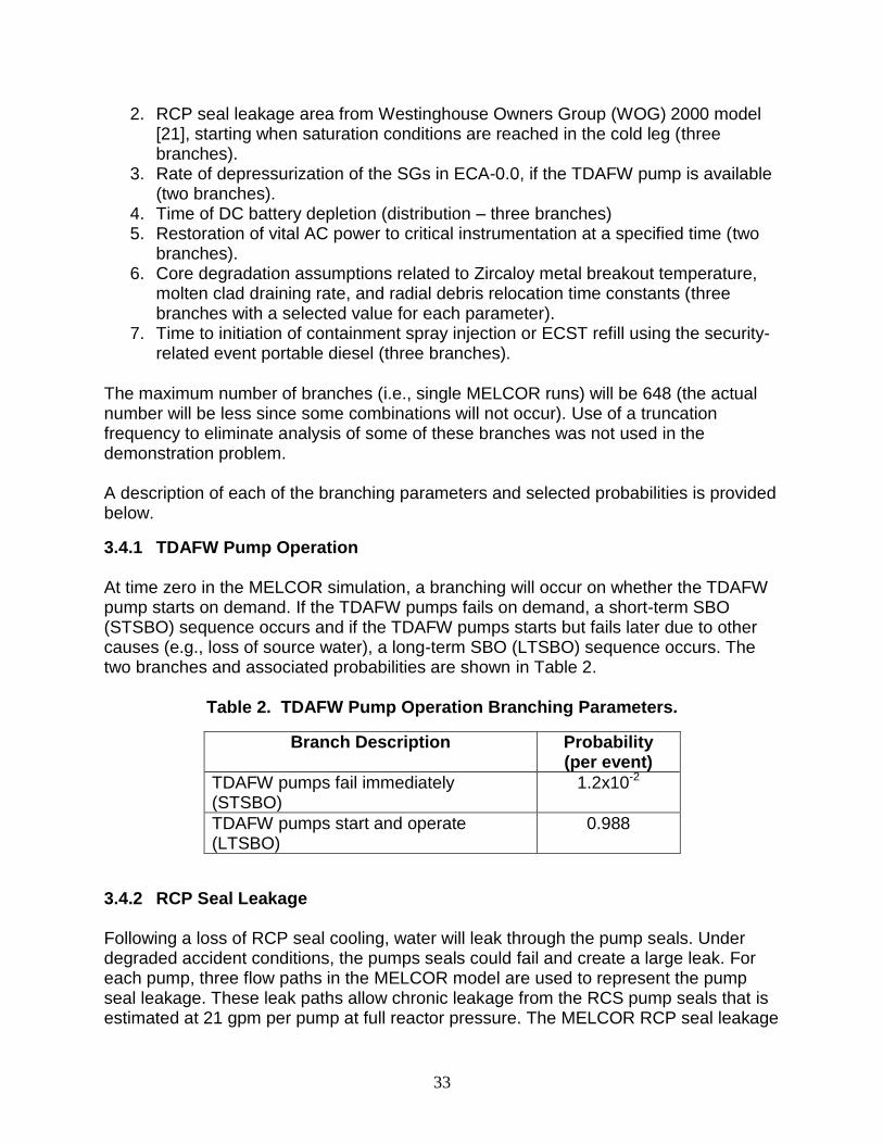
33

2. RCP seal leakage area from Westinghouse Owners Group (WOG) 2000 model [21], starting when saturation conditions are reached in the cold leg (three branches).

3. Rate of depressurization of the SGs in ECA-0.0, if the TDAFW pump is available (two branches).

4. Time of DC battery depletion (distribution – three branches) 5. Restoration of vital AC power to critical instrumentation at a specified time (two

branches). 6. Core degradation assumptions related to Zircaloy metal breakout temperature,

molten clad draining rate, and radial debris relocation time constants (three branches with a selected value for each parameter).

7. Time to initiation of containment spray injection or ECST refill using the security-related event portable diesel (three branches).

The maximum number of branches (i.e., single MELCOR runs) will be 648 (the actual number will be less since some combinations will not occur). Use of a truncation frequency to eliminate analysis of some of these branches was not used in the demonstration problem. A description of each of the branching parameters and selected probabilities is provided below.

3.4.1 TDAFW Pump Operation At time zero in the MELCOR simulation, a branching will occur on whether the TDAFW pump starts on demand. If the TDAFW pumps fails on demand, a short-term SBO (STSBO) sequence occurs and if the TDAFW pumps starts but fails later due to other causes (e.g., loss of source water), a long-term SBO (LTSBO) sequence occurs. The two branches and associated probabilities are shown in Table 2.

Table 2. TDAFW Pump Operation Branching Parameters.

Branch Description Probability (per event)

TDAFW pumps fail immediately (STSBO)

1.2x10-2

TDAFW pumps start and operate (LTSBO)

0.988

3.4.2 RCP Seal Leakage Following a loss of RCP seal cooling, water will leak through the pump seals. Under degraded accident conditions, the pumps seals could fail and create a large leak. For each pump, three flow paths in the MELCOR model are used to represent the pump seal leakage. These leak paths allow chronic leakage from the RCS pump seals that is estimated at 21 gpm per pump at full reactor pressure. The MELCOR RCP seal leakage

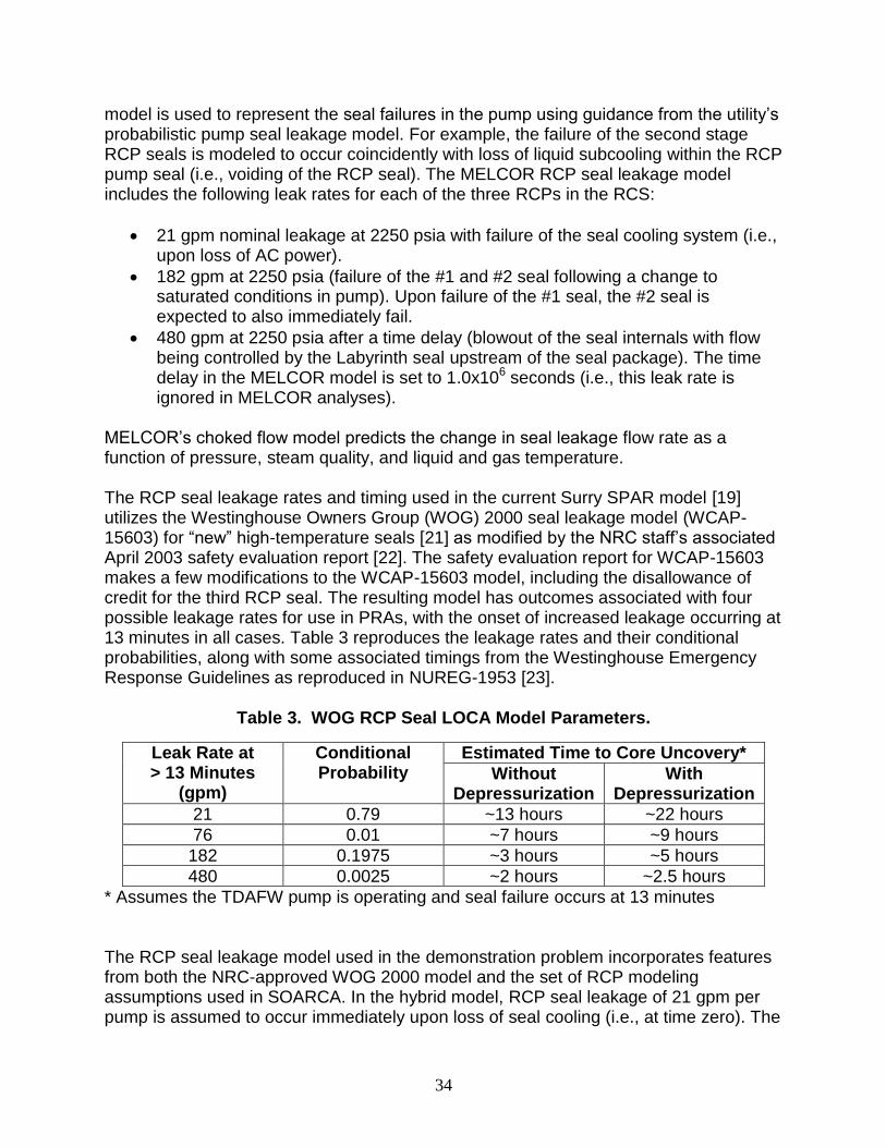
34

model is used to represent the seal failures in the pump using guidance from the utility’s probabilistic pump seal leakage model. For example, the failure of the second stage RCP seals is modeled to occur coincidently with loss of liquid subcooling within the RCP pump seal (i.e., voiding of the RCP seal). The MELCOR RCP seal leakage model includes the following leak rates for each of the three RCPs in the RCS:

21 gpm nominal leakage at 2250 psia with failure of the seal cooling system (i.e., upon loss of AC power).

182 gpm at 2250 psia (failure of the #1 and #2 seal following a change to saturated conditions in pump). Upon failure of the #1 seal, the #2 seal is expected to also immediately fail.

480 gpm at 2250 psia after a time delay (blowout of the seal internals with flow being controlled by the Labyrinth seal upstream of the seal package). The time delay in the MELCOR model is set to 1.0x106 seconds (i.e., this leak rate is ignored in MELCOR analyses).

MELCOR’s choked flow model predicts the change in seal leakage flow rate as a function of pressure, steam quality, and liquid and gas temperature. The RCP seal leakage rates and timing used in the current Surry SPAR model [19] utilizes the Westinghouse Owners Group (WOG) 2000 seal leakage model (WCAP-15603) for “new” high-temperature seals [21] as modified by the NRC staff’s associated April 2003 safety evaluation report [22]. The safety evaluation report for WCAP-15603 makes a few modifications to the WCAP-15603 model, including the disallowance of credit for the third RCP seal. The resulting model has outcomes associated with four possible leakage rates for use in PRAs, with the onset of increased leakage occurring at 13 minutes in all cases. Table 3 reproduces the leakage rates and their conditional probabilities, along with some associated timings from the Westinghouse Emergency Response Guidelines as reproduced in NUREG-1953 [23].

Table 3. WOG RCP Seal LOCA Model Parameters.

Leak Rate at > 13 Minutes

(gpm)

Conditional Probability

Estimated Time to Core Uncovery*

Without Depressurization

With Depressurization

21 0.79 ~13 hours ~22 hours

76 0.01 ~7 hours ~9 hours

182 0.1975 ~3 hours ~5 hours

480 0.0025 ~2 hours ~2.5 hours

* Assumes the TDAFW pump is operating and seal failure occurs at 13 minutes The RCP seal leakage model used in the demonstration problem incorporates features from both the NRC-approved WOG 2000 model and the set of RCP modeling assumptions used in SOARCA. In the hybrid model, RCP seal leakage of 21 gpm per pump is assumed to occur immediately upon loss of seal cooling (i.e., at time zero). The

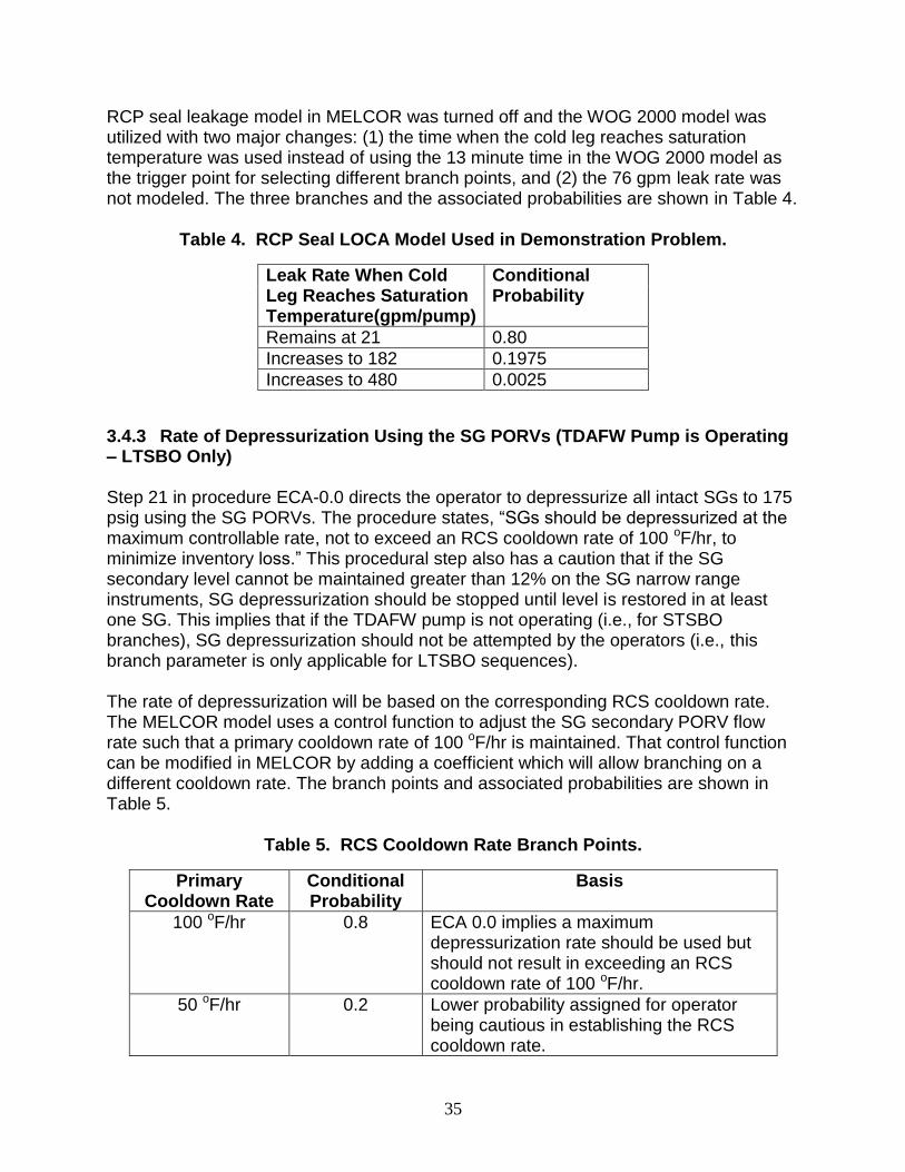
35

RCP seal leakage model in MELCOR was turned off and the WOG 2000 model was utilized with two major changes: (1) the time when the cold leg reaches saturation temperature was used instead of using the 13 minute time in the WOG 2000 model as the trigger point for selecting different branch points, and (2) the 76 gpm leak rate was not modeled. The three branches and the associated probabilities are shown in Table 4.

Table 4. RCP Seal LOCA Model Used in Demonstration Problem.

Leak Rate When Cold Leg Reaches Saturation Temperature(gpm/pump)


Remains at 21 0.80

Increases to 182 0.1975

Increases to 480 0.0025

3.4.3 Rate of Depressurization Using the SG PORVs (TDAFW Pump is Operating – LTSBO Only) Step 21 in procedure ECA-0.0 directs the operator to depressurize all intact SGs to 175 psig using the SG PORVs. The procedure states, “SGs should be depressurized at the maximum controllable rate, not to exceed an RCS cooldown rate of 100 oF/hr, to minimize inventory loss.” This procedural step also has a caution that if the SG secondary level cannot be maintained greater than 12% on the SG narrow range instruments, SG depressurization should be stopped until level is restored in at least one SG. This implies that if the TDAFW pump is not operating (i.e., for STSBO branches), SG depressurization should not be attempted by the operators (i.e., this branch parameter is only applicable for LTSBO sequences). The rate of depressurization will be based on the corresponding RCS cooldown rate. The MELCOR model uses a control function to adjust the SG secondary PORV flow rate such that a primary cooldown rate of 100 oF/hr is maintained. That control function can be modified in MELCOR by adding a coefficient which will allow branching on a different cooldown rate. The branch points and associated probabilities are shown in Table 5.

Table 5. RCS Cooldown Rate Branch Points.

Primary Cooldown Rate


Basis

100 oF/hr 0.8 ECA 0.0 implies a maximum depressurization rate should be used but should not result in exceeding an RCS cooldown rate of 100 oF/hr.

50 oF/hr 0.2 Lower probability assigned for operator being cautious in establishing the RCS cooldown rate.

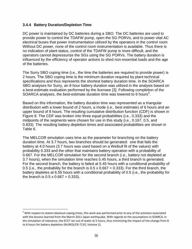
36

3.4.4 Battery Duration/Depletion Time DC power is maintained by DC batteries during a SBO. The DC batteries are used to provide power to control the TDAFW pump, open the SG PORVs, and to power vital AC electrical buses that power instrumentation utilized by the operators in the control room. Without DC power, none of the control room instrumentation is available. Thus there is no indication of plant status, control of the TDAFW pump is more difficult, and the operators cannot depressurize the SGs using the SG PORVs. The battery duration is influenced by the efficiency of operator actions to shed non-essential loads and the age of the batteries. The Surry SBO coping time (i.e., the time the batteries are required to provide power) is 2 hours. The SBO coping time is the minimum duration required by plant technical specifications and thus represents the shortest battery duration time. In the SOARCA SBO analyses for Surry, an 8 hour battery duration was utilized in the analysis based on a best-estimate evaluation performed by the licensee [3]. Following completion of the SOARCA analyses, the best-estimate duration time was lowered to 6 hours4. Based on this information, the battery duration time was represented as a triangular distribution with a lower bound of 2 hours, a mode (i.e., best estimate) of 6 hours and an upper bound of 8 hours. The resulting cumulative distribution function (CDF) is shown in Figure 8. The CDF was broken into three equal probabilities (i.e., 0.333) and the midpoints of the segments were chosen for use in this study (i.e., 0.167, 0.5, and 0.833). The resulting battery depletion times and associated probabilities are shown in Table 6. The MELCOR simulation uses time as the parameter for branching on the battery duration time. At 3.7 hours, two branches should be generated: one that fails the battery at 4.0 hours (3.7 hours was used based on a Weibull fit of the values) with probability 0.333 and the other that maintains battery operation with a probability of 0.667. For the MELCOR simulation for the second branch (i.e., battery not depleted at 3.7 hours), when the simulation time reaches 5.45 hours, a third branch is generated. For the second branch, the battery is failed at 5.45 hours with a conditional probability of 0.5 (i.e., the probability for the branch is 0.5 x 0.667 = 0.333). For the third branch, the battery depletes at 6.55 hours with a conditional probability of 0.5 (i.e., the probability for the branch is 0.5 x 0.667 = 0.333).

4 With respect to station blackout coping times, this work was performed prior to any of the activities associated

with the lessons-learned from the March 2011 Japan earthquake. With regards to the assumptions in SOARCA, in the simulation of relevance, the ECST ran out of water at 5 hours, thus minimizing the impact of the change from 8 to 6 hours for battery depletion (NUREG/CR-7110, Volume 2).

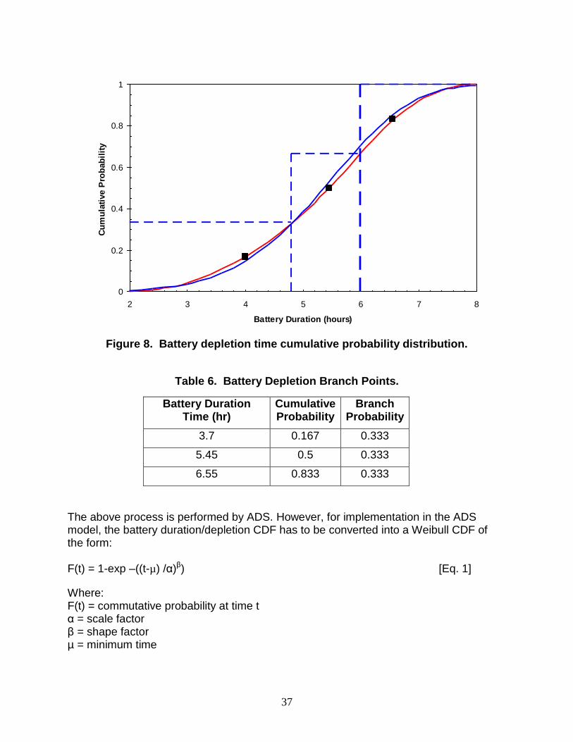
37

Figure 8. Battery depletion time cumulative probability distribution.

Table 6. Battery Depletion Branch Points.

Battery Duration Time (hr)

Cumulative Probability

Branch Probability

3.7 0.167 0.333

5.45 0.5 0.333

6.55 0.833 0.333

The above process is performed by ADS. However, for implementation in the ADS model, the battery duration/depletion CDF has to be converted into a Weibull CDF of the form: F(t) = 1-exp –((t-µ) /α)β) [Eq. 1]

Where: F(t) = commutative probability at time t α = scale factor β = shape factor µ = minimum time

0

0.2

0.4

0.6

0.8

1

2 3 4 5 6 7 8

Battery Duration (hours)

Cu

mu

lati

ve P

rob

ab

ilit

y

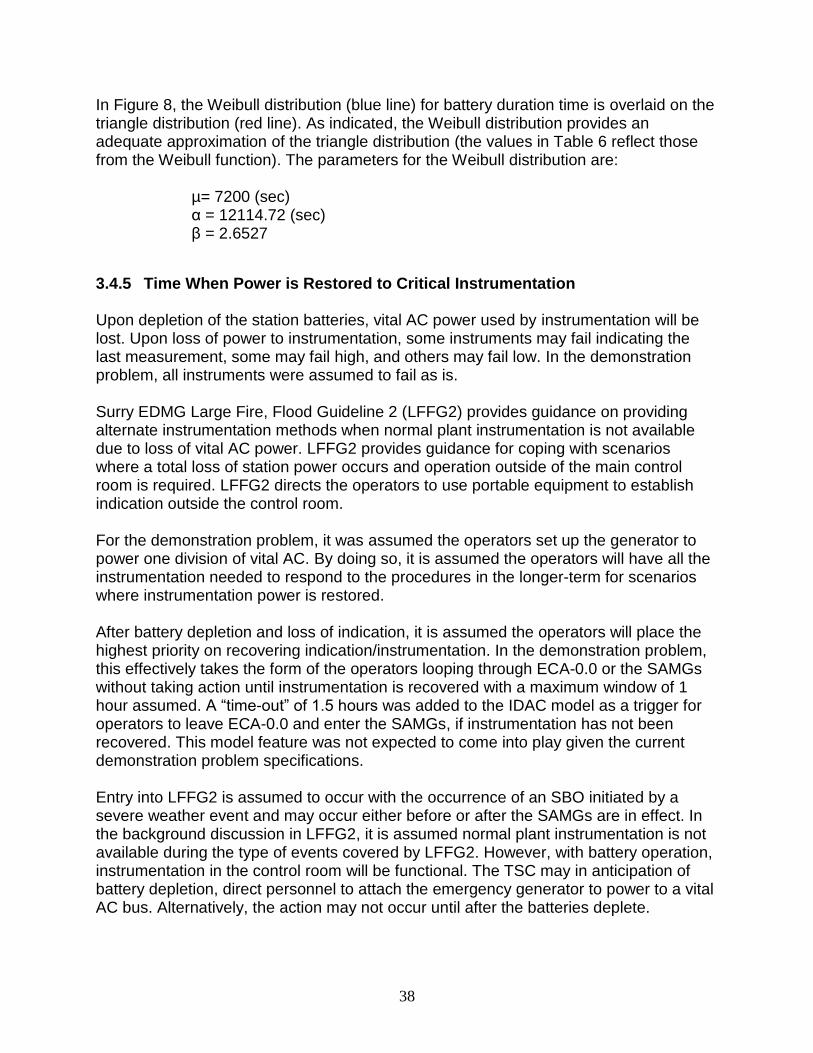
38

In Figure 8, the Weibull distribution (blue line) for battery duration time is overlaid on the triangle distribution (red line). As indicated, the Weibull distribution provides an adequate approximation of the triangle distribution (the values in Table 6 reflect those from the Weibull function). The parameters for the Weibull distribution are:

µ= 7200 (sec) α = 12114.72 (sec) β = 2.6527

3.4.5 Time When Power is Restored to Critical Instrumentation

Upon depletion of the station batteries, vital AC power used by instrumentation will be lost. Upon loss of power to instrumentation, some instruments may fail indicating the last measurement, some may fail high, and others may fail low. In the demonstration problem, all instruments were assumed to fail as is. Surry EDMG Large Fire, Flood Guideline 2 (LFFG2) provides guidance on providing alternate instrumentation methods when normal plant instrumentation is not available due to loss of vital AC power. LFFG2 provides guidance for coping with scenarios where a total loss of station power occurs and operation outside of the main control room is required. LFFG2 directs the operators to use portable equipment to establish indication outside the control room. For the demonstration problem, it was assumed the operators set up the generator to power one division of vital AC. By doing so, it is assumed the operators will have all the instrumentation needed to respond to the procedures in the longer-term for scenarios where instrumentation power is restored. After battery depletion and loss of indication, it is assumed the operators will place the highest priority on recovering indication/instrumentation. In the demonstration problem, this effectively takes the form of the operators looping through ECA-0.0 or the SAMGs without taking action until instrumentation is recovered with a maximum window of 1 hour assumed. A “time-out” of 1.5 hours was added to the IDAC model as a trigger for operators to leave ECA-0.0 and enter the SAMGs, if instrumentation has not been recovered. This model feature was not expected to come into play given the current demonstration problem specifications. Entry into LFFG2 is assumed to occur with the occurrence of an SBO initiated by a severe weather event and may occur either before or after the SAMGs are in effect. In the background discussion in LFFG2, it is assumed normal plant instrumentation is not available during the type of events covered by LFFG2. However, with battery operation, instrumentation in the control room will be functional. The TSC may in anticipation of battery depletion, direct personnel to attach the emergency generator to power to a vital AC bus. Alternatively, the action may not occur until after the batteries deplete.

39

The times and associated probabilities for aligning the portable generator to the vital AC bus are provided in Table 7.

Table 7. Power Restoration to Instrumentation Branching Parameters.

Time When Portable

Generator is Connected to

Remote Monitoring Panel*


Assumptions

3 hours after accident initiation (2 hours after manning the TSC)

0.2

After the TSC is manned (assumed to occur at 1 hour), personnel will review the situation and enter LFFG2. In anticipation of battery depletion, they make the decision at hour 3 to align the portable generator as a precautionary measure. Alignment is assumed to take 1 hour

1 hour after battery depletion

0.8

After battery depletion, instrumentation will be lost and the TSC will direct personnel to align the generator per LFFG2. Alignment is assumed to take 1 hour

*These timings are intended to be for illustrative purposes; they are not the result of a detailed task analysis

At 2 hours into the accident, a branching decision will be made. The first sequence will assume portable power is connected to the Remote Monitoring Panel at 3 hours (i.e., prior to battery depletion and loss of instrumentation) with a probability of 0.2. The second branch assumes the action does not take place until 1 hour after battery depletion and loss of instrumentation with a probability of 0.8.

3.4.6 In-Vessel Accident Progression Phenomena Three in-vessel accident progression parameters that have an important impact on the severe accident progression predicted by MELCOR are combined together as a single branching parameter. They are:

Zircaloy Metal Breakout Temperature

Molten Cladding Drainage Rate

Radial Debris Location Time Constants Each of these parameters is described below along with the selected branching probabilities.

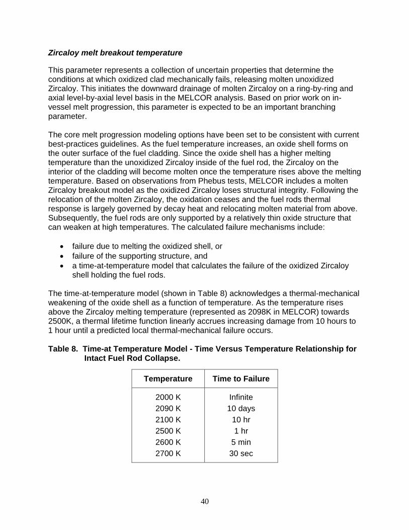
40

Zircaloy melt breakout temperature

This parameter represents a collection of uncertain properties that determine the conditions at which oxidized clad mechanically fails, releasing molten unoxidized Zircaloy. This initiates the downward drainage of molten Zircaloy on a ring-by-ring and axial level-by-axial level basis in the MELCOR analysis. Based on prior work on in-vessel melt progression, this parameter is expected to be an important branching parameter. The core melt progression modeling options have been set to be consistent with current best-practices guidelines. As the fuel temperature increases, an oxide shell forms on the outer surface of the fuel cladding. Since the oxide shell has a higher melting temperature than the unoxidized Zircaloy inside of the fuel rod, the Zircaloy on the interior of the cladding will become molten once the temperature rises above the melting temperature. Based on observations from Phebus tests, MELCOR includes a molten Zircaloy breakout model as the oxidized Zircaloy loses structural integrity. Following the relocation of the molten Zircaloy, the oxidation ceases and the fuel rods thermal response is largely governed by decay heat and relocating molten material from above. Subsequently, the fuel rods are only supported by a relatively thin oxide structure that can weaken at high temperatures. The calculated failure mechanisms include:

failure due to melting the oxidized shell, or

failure of the supporting structure, and

a time-at-temperature model that calculates the failure of the oxidized Zircaloy shell holding the fuel rods.

The time-at-temperature model (shown in Table 8) acknowledges a thermal-mechanical weakening of the oxide shell as a function of temperature. As the temperature rises above the Zircaloy melting temperature (represented as 2098K in MELCOR) towards 2500K, a thermal lifetime function linearly accrues increasing damage from 10 hours to 1 hour until a predicted local thermal-mechanical failure occurs. Table 8. Time-at Temperature Model - Time Versus Temperature Relationship for

Intact Fuel Rod Collapse.

Temperature Time to Failure

2000 K

2090 K

2100 K

2500 K

2600 K

2700 K

Infinite

10 days

10 hr

1 hr

5 min

30 sec

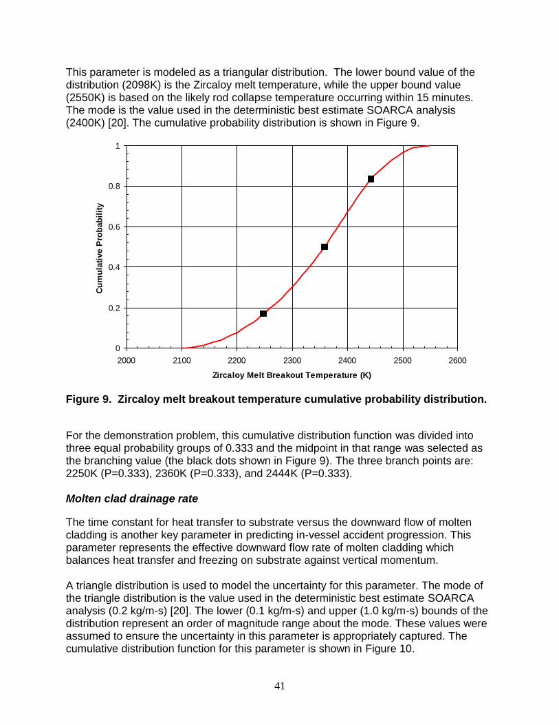
41

This parameter is modeled as a triangular distribution. The lower bound value of the distribution (2098K) is the Zircaloy melt temperature, while the upper bound value (2550K) is based on the likely rod collapse temperature occurring within 15 minutes. The mode is the value used in the deterministic best estimate SOARCA analysis (2400K) [20]. The cumulative probability distribution is shown in Figure 9.

Figure 9. Zircaloy melt breakout temperature cumulative probability distribution.

For the demonstration problem, this cumulative distribution function was divided into three equal probability groups of 0.333 and the midpoint in that range was selected as the branching value (the black dots shown in Figure 9). The three branch points are: 2250K (P=0.333), 2360K (P=0.333), and 2444K (P=0.333). Molten clad drainage rate

The time constant for heat transfer to substrate versus the downward flow of molten cladding is another key parameter in predicting in-vessel accident progression. This parameter represents the effective downward flow rate of molten cladding which balances heat transfer and freezing on substrate against vertical momentum. A triangle distribution is used to model the uncertainty for this parameter. The mode of the triangle distribution is the value used in the deterministic best estimate SOARCA analysis (0.2 kg/m-s) [20]. The lower (0.1 kg/m-s) and upper (1.0 kg/m-s) bounds of the distribution represent an order of magnitude range about the mode. These values were assumed to ensure the uncertainty in this parameter is appropriately captured. The cumulative distribution function for this parameter is shown in Figure 10.

0

0.2

0.4

0.6

0.8

1

2000 2100 2200 2300 2400 2500 2600

Zircaloy Melt Breakout Temperature (K)

Cu

mu

lati

ve P

rob

ab

ilit

y

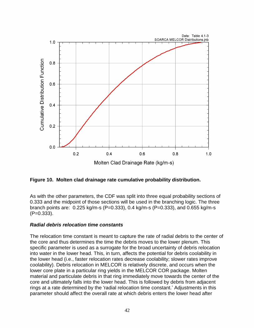
42

Figure 10. Molten clad drainage rate cumulative probability distribution.

As with the other parameters, the CDF was split into three equal probability sections of 0.333 and the midpoint of those sections will be used in the branching logic. The three branch points are: 0.225 kg/m-s (P=0.333), 0.4 kg/m-s (P=0.333), and 0.655 kg/m-s (P=0.333). Radial debris relocation time constants The relocation time constant is meant to capture the rate of radial debris to the center of the core and thus determines the time the debris moves to the lower plenum. This specific parameter is used as a surrogate for the broad uncertainty of debris relocation into water in the lower head. This, in turn, affects the potential for debris coolability in the lower head (i.e., faster relocation rates decrease coolability; slower rates improve coolability). Debris relocation in MELCOR is relatively discrete, and occurs when the lower core plate in a particular ring yields in the MELCOR COR package. Molten material and particulate debris in that ring immediately move towards the center of the core and ultimately falls into the lower head. This is followed by debris from adjacent rings at a rate determined by the 'radial relocation time constant.’ Adjustments in this parameter should affect the overall rate at which debris enters the lower head after

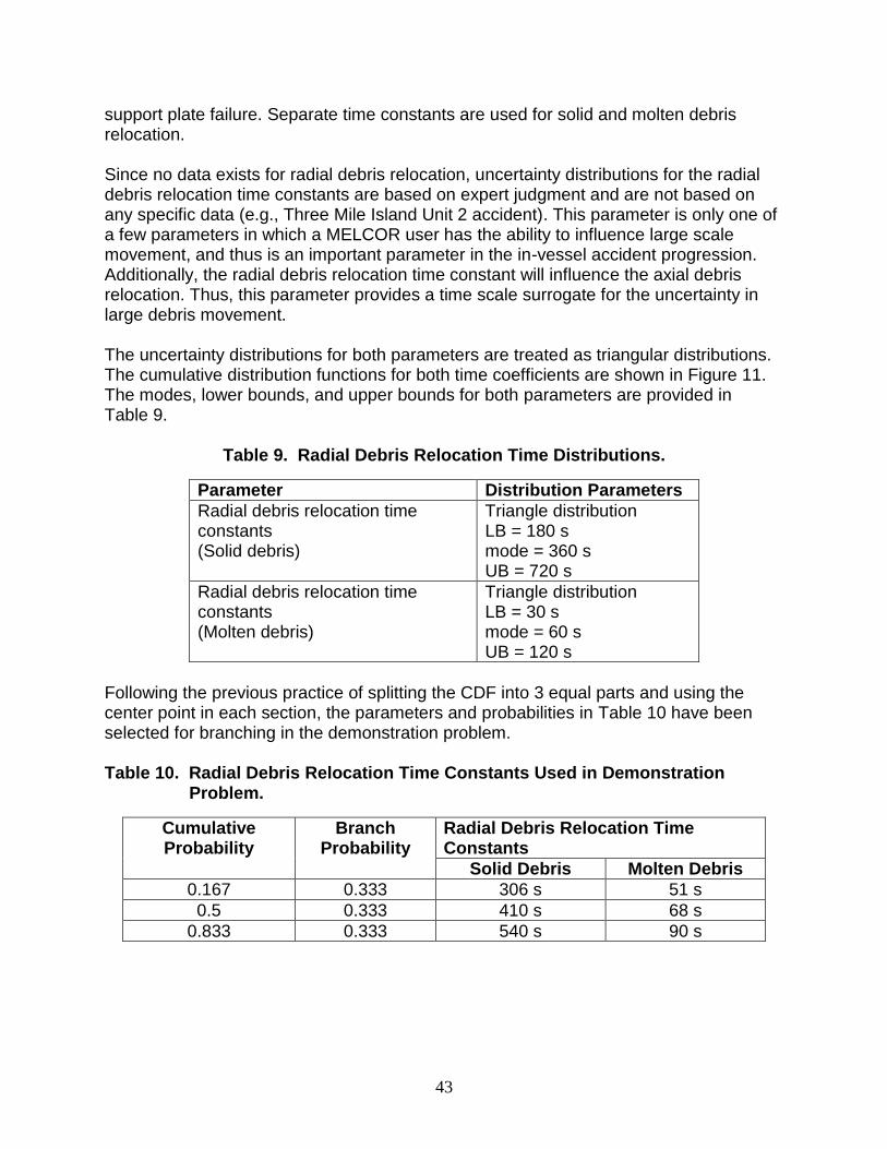
43

support plate failure. Separate time constants are used for solid and molten debris relocation. Since no data exists for radial debris relocation, uncertainty distributions for the radial debris relocation time constants are based on expert judgment and are not based on any specific data (e.g., Three Mile Island Unit 2 accident). This parameter is only one of a few parameters in which a MELCOR user has the ability to influence large scale movement, and thus is an important parameter in the in-vessel accident progression. Additionally, the radial debris relocation time constant will influence the axial debris relocation. Thus, this parameter provides a time scale surrogate for the uncertainty in large debris movement. The uncertainty distributions for both parameters are treated as triangular distributions. The cumulative distribution functions for both time coefficients are shown in Figure 11. The modes, lower bounds, and upper bounds for both parameters are provided in Table 9.

Table 9. Radial Debris Relocation Time Distributions.

Parameter Distribution Parameters

Radial debris relocation time constants (Solid debris)

Triangle distribution LB = 180 s mode = 360 s UB = 720 s

Radial debris relocation time constants (Molten debris)

Triangle distribution LB = 30 s mode = 60 s UB = 120 s

Following the previous practice of splitting the CDF into 3 equal parts and using the center point in each section, the parameters and probabilities in Table 10 have been selected for branching in the demonstration problem. Table 10. Radial Debris Relocation Time Constants Used in Demonstration

Problem.

Cumulative Probability

Branch Probability

Radial Debris Relocation Time Constants

Solid Debris Molten Debris

0.167 0.333 306 s 51 s

0.5 0.333 410 s 68 s

0.833 0.333 540 s 90 s

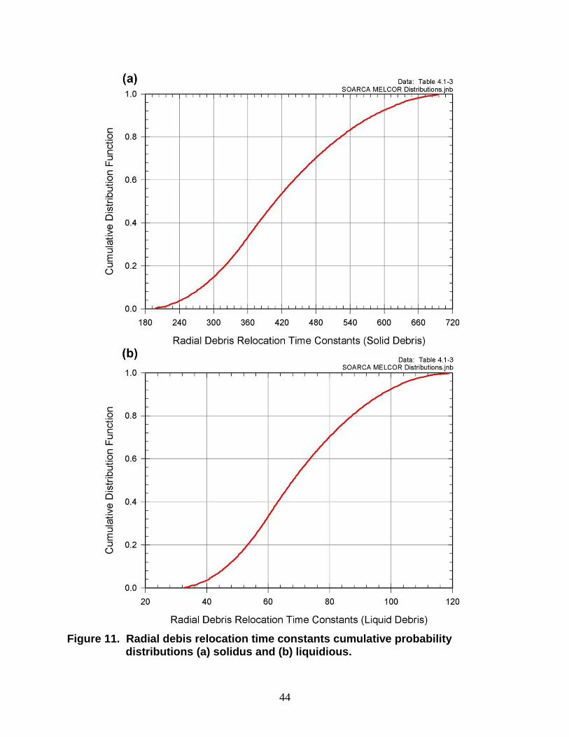
44

Figure 11. Radial debis relocation time constants cumulative probability distributions (a) solidus and (b) liquidious.

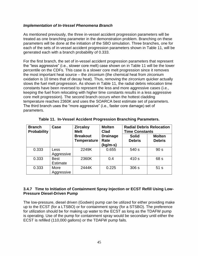
45

Implementation of In-Vessel Phenomena Branch As mentioned previously, the three in-vessel accident progression parameters will be treated as one branching parameter in the demonstration problem. Branching on these parameters will be done at the initiation of the SBO simulation. Three branches, one for each of the sets of in-vessel accident progression parameters shown in Table 11, will be generated each with a branch probability of 0.333. For the first branch, the set of in-vessel accident progression parameters that represent the “less aggressive” (i.e., slower core melt) case shown on in Table 11 will be the lower percentile on the CDFs. This case is a slower core melt progression since it removes the most important heat source – the zirconium (the chemical heat from zirconium oxidation is 10 times that of decay heat). Thus, removing the zirconium quicker actually slows the fuel melt progression. As shown in Table 11, the radial debris relocation time constants have been reversed to represent the less and more aggressive cases (i.e., keeping the fuel from relocating with higher time constants results in a less aggressive core melt progression). The second branch occurs when the hottest cladding temperature reaches 2360K and uses the SOARCA best estimate set of parameters. The third branch uses the “more aggressive” (i.e., faster core damage) set of parameters.

Table 11. In-Vessel Accident Progression Branching Parameters.

Branch Probability

Case Zircaloy Melt Breakout Temperature

Molten Clad Drainage Rate (kg/m-s)

Radial Debris Relocation Time Constants

Solid Debris

Molten Debris

0.333 Less Aggressive

2249K 0.655 540 s 90 s

0.333 Best Estimate

2360K 0.4 410 s 68 s

0.333 More Aggressive

2444K 0.225 306 s 51 s

3.4.7 Time to Initiation of Containment Spray Injection or ECST Refill Using Low-Pressure Diesel-Driven Pump The low-pressure, diesel driven (Godwin) pump can be utilized for either providing make up to the ECST (for a LTSBO) or for containment spray (for a STSBO). The preference for utilization should be for making up water to the ECST as long as the TDAFW pump is operating. Use of the pump for containment spray would be secondary until either the ECST is refilled (110,000 gallons) or the TDAFW pump fails.

46

The time to transport the pump and connect it to the appropriate plant piping is assumed to take two hours. This is assumed to be the nominal value. The CDF for the time to implement this is shown in Table 12 and assumes the minimum and maximum implementation time is one and three hours, respectively, after the decision is made.

Table 12. Containment Spray Initiation Branching Parameters.

Time to Implementation Branch Probability

One hour after decision is made to utilize the pump

0.333

Two hours after decision is made to utilize the pump

0.333

Three hours after decision is made to utilize the pump

0.333

47

4. DISCRETE DYNAMIC PRA TOOL DEVELOPMENT

4.1 ADS-IDAC Model for Demonstration Problem An ADS simulation input model was developed for the selected demonstration problem, including the initiating event, conditional failure settings, operator profiles, procedures, guidance, and calculation aids. ADS provides users the flexibility of designing simulation scenarios by setting the initiating event and the hardware failure events in the input model. The demonstration simulation starts with a SBO as the initiating event. This is “hard coded” in the MELCOR input model. However, ADS also has the capability of sending an order to the plant hardware model to initiate the SBO by setting it in the input file “Initiating_Event.txt”. In the demonstration scenario, the TDAFW pump fails on demand with a certain probability. This is also set in the input file “SystemReliability.txt”. In addition to TDAFW pump failure, several other hardware dynamics are present in the demonstration scenario. They are: battery depletion, RCP seal leakage degradation, and restoration of vital AC power to critical instrumentation. ADS could set up time-based hardware actions in the “Initiating_Event.txt” file (e.g., let the battery deplete at a specific time). But this would not generate branches for different times. So the branching of different battery depletion times is modeled in another way through the IDAC “operator mental belief,” which is discussed later in this section. While the “Initiating_Event.txt” file allows the user to set up some time-based hardware activities, the “SystemReliability.txt” file allows the user to design some hardware activities with certain conditions. Each hardware state in the “SystemReliability.txt” file has a specific condition to be triggered, generating binary branching with assigned probabilities: (1) Happens and (2) Does Not Happen. The RCP seal leakage modeled in the demonstration scenario however has three states. To handle non-binary states in the “Initiating_Event.txt” and “SystemReliability.txt” files, the triggering logic for battery depletion, RCP seal leakage, and restoration of vital AC power were built using the operator’s mental beliefs and mental procedures.5 During the accident scenario, the operators’ behaviors are determined by two sets of factors: the operators’ mental model (knowledge and situation awareness), and external input (procedures and calculation aids). Building the operators knowledge model and the use of procedures and calculation aids is the key part of preparing the ADS-IDAC input model. Figure 12 shows the structure of the input crew model [24]. Coding the procedural steps, calculation aids, and operators’ knowledge base were major additions to the IDAC

5 Mental beliefs represent discrete decisions or observations and serve as the basic decision-making building blocks

in ADS-IDAC. Written procedures represent formal proceduralized guidance contained in normal, abnormal, and emergency operating procedures. Memorized mental procedures represent the skill- and rule-based actions routinely used by the operators that do not require formal procedure guidance.

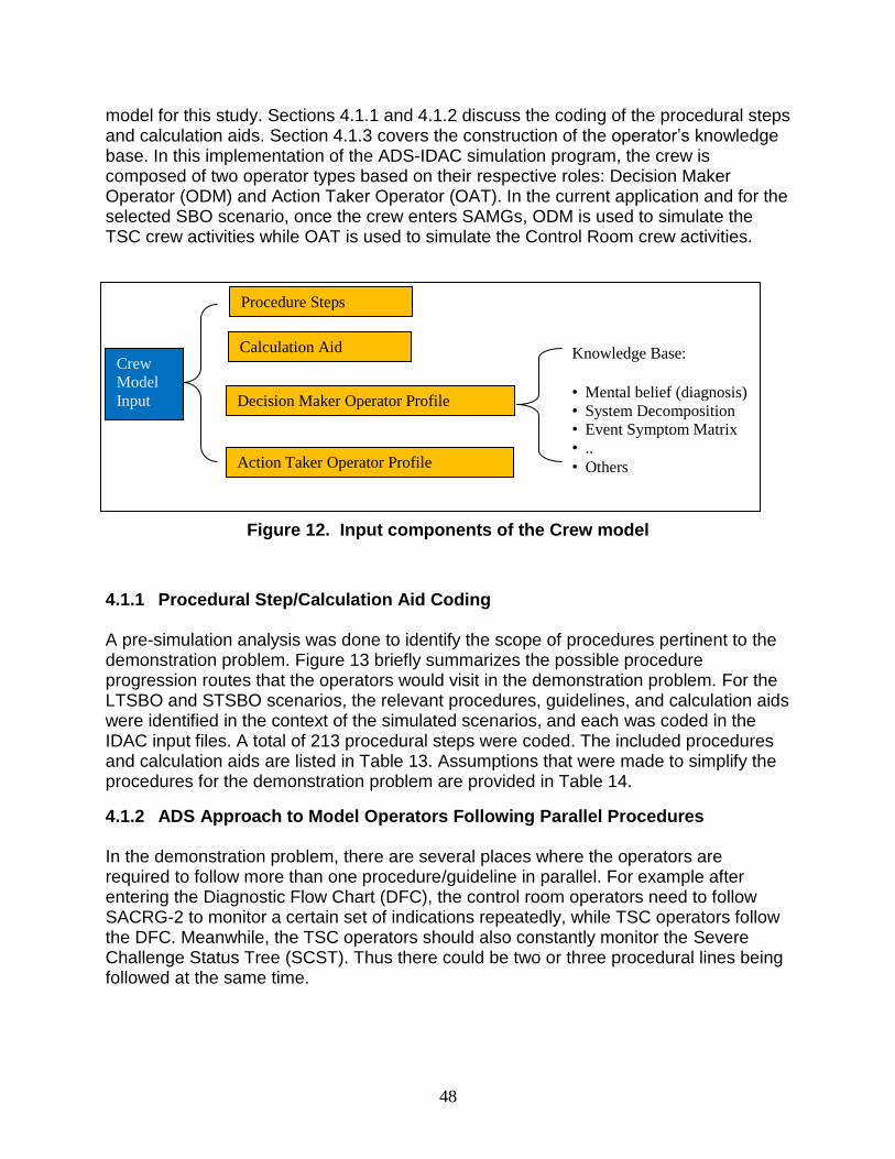
48

model for this study. Sections 4.1.1 and 4.1.2 discuss the coding of the procedural steps and calculation aids. Section 4.1.3 covers the construction of the operator’s knowledge base. In this implementation of the ADS-IDAC simulation program, the crew is composed of two operator types based on their respective roles: Decision Maker Operator (ODM) and Action Taker Operator (OAT). In the current application and for the selected SBO scenario, once the crew enters SAMGs, ODM is used to simulate the TSC crew activities while OAT is used to simulate the Control Room crew activities.

Figure 12. Input components of the Crew model

4.1.1 Procedural Step/Calculation Aid Coding A pre-simulation analysis was done to identify the scope of procedures pertinent to the demonstration problem. Figure 13 briefly summarizes the possible procedure progression routes that the operators would visit in the demonstration problem. For the LTSBO and STSBO scenarios, the relevant procedures, guidelines, and calculation aids were identified in the context of the simulated scenarios, and each was coded in the IDAC input files. A total of 213 procedural steps were coded. The included procedures and calculation aids are listed in Table 13. Assumptions that were made to simplify the procedures for the demonstration problem are provided in Table 14.

4.1.2 ADS Approach to Model Operators Following Parallel Procedures In the demonstration problem, there are several places where the operators are required to follow more than one procedure/guideline in parallel. For example after entering the Diagnostic Flow Chart (DFC), the control room operators need to follow SACRG-2 to monitor a certain set of indications repeatedly, while TSC operators follow the DFC. Meanwhile, the TSC operators should also constantly monitor the Severe Challenge Status Tree (SCST). Thus there could be two or three procedural lines being followed at the same time.

Crew

Model

Input

Procedure Steps

Decision Maker Operator Profile

Action Taker Operator Profile

Calculation Aid Knowledge Base:

• Mental belief (diagnosis)

• System Decomposition

• Event Symptom Matrix

• ..

• Others

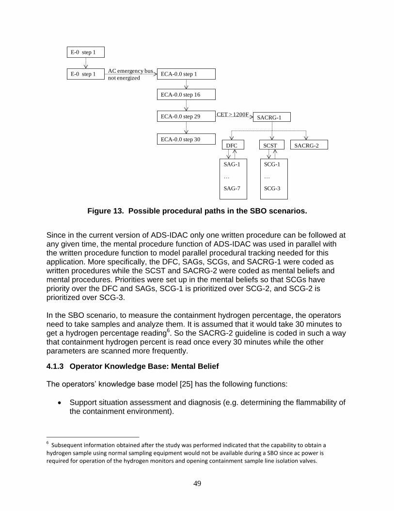
49

Figure 13. Possible procedural paths in the SBO scenarios.

Since in the current version of ADS-IDAC only one written procedure can be followed at any given time, the mental procedure function of ADS-IDAC was used in parallel with the written procedure function to model parallel procedural tracking needed for this application. More specifically, the DFC, SAGs, SCGs, and SACRG-1 were coded as written procedures while the SCST and SACRG-2 were coded as mental beliefs and mental procedures. Priorities were set up in the mental beliefs so that SCGs have priority over the DFC and SAGs, SCG-1 is prioritized over SCG-2, and SCG-2 is prioritized over SCG-3. In the SBO scenario, to measure the containment hydrogen percentage, the operators need to take samples and analyze them. It is assumed that it would take 30 minutes to get a hydrogen percentage reading6. So the SACRG-2 guideline is coded in such a way that containment hydrogen percent is read once every 30 minutes while the other parameters are scanned more frequently.

4.1.3 Operator Knowledge Base: Mental Belief The operators’ knowledge base model [25] has the following functions:

Support situation assessment and diagnosis (e.g. determining the flammability of the containment environment).

6 Subsequent information obtained after the study was performed indicated that the capability to obtain a

hydrogen sample using normal sampling equipment would not be available during a SBO since ac power is required for operation of the hydrogen monitors and opening containment sample line isolation valves.

E-0 step 1

ECA-0.0 step 30

ECA-0.0 step 1

ECA-0.0 step 16

ECA-0.0 step 29

AC emergency bus

not energized

SCSTDFC

SACRG-1

SACRG-2

E-0 step 1

CET > 1200F

SAG-1

…

SAG-7

SCG-1

…

SCG-3

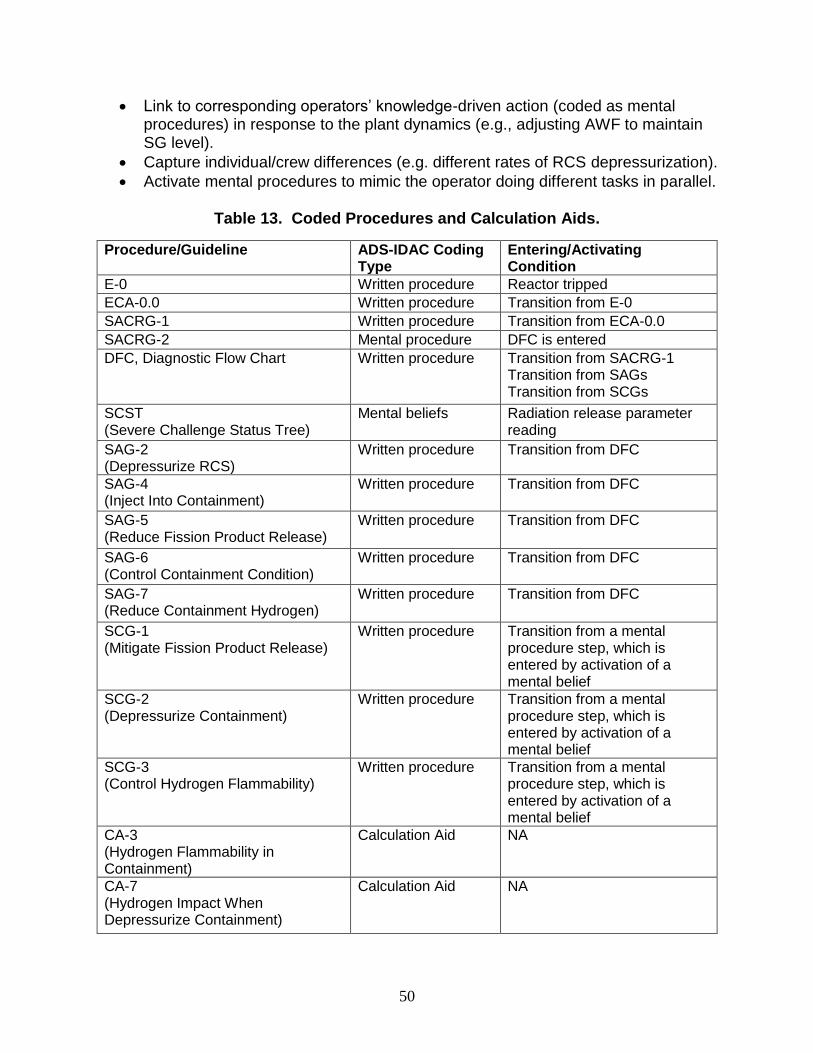
50

Link to corresponding operators’ knowledge-driven action (coded as mental procedures) in response to the plant dynamics (e.g., adjusting AWF to maintain SG level).

Capture individual/crew differences (e.g. different rates of RCS depressurization).

Activate mental procedures to mimic the operator doing different tasks in parallel.

Table 13. Coded Procedures and Calculation Aids.

Procedure/Guideline ADS-IDAC Coding Type

Entering/Activating Condition

E-0 Written procedure Reactor tripped

ECA-0.0 Written procedure Transition from E-0

SACRG-1 Written procedure Transition from ECA-0.0

SACRG-2 Mental procedure DFC is entered

DFC, Diagnostic Flow Chart Written procedure Transition from SACRG-1 Transition from SAGs Transition from SCGs

SCST (Severe Challenge Status Tree)

Mental beliefs Radiation release parameter reading

SAG-2 (Depressurize RCS)

Written procedure Transition from DFC

SAG-4 (Inject Into Containment)


SAG-5 (Reduce Fission Product Release)


SAG-6 (Control Containment Condition)


SAG-7 (Reduce Containment Hydrogen)


SCG-1 (Mitigate Fission Product Release)

Written procedure Transition from a mental procedure step, which is entered by activation of a mental belief

SCG-2 (Depressurize Containment)


SCG-3 (Control Hydrogen Flammability)


CA-3 (Hydrogen Flammability in Containment)

Calculation Aid NA

CA-7 (Hydrogen Impact When Depressurize Containment)

Calculation Aid NA

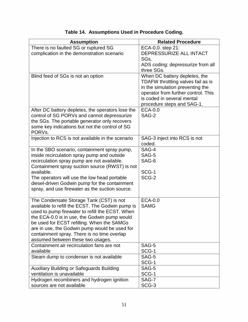
51

Table 14. Assumptions Used in Procedure Coding.

Assumption Related Procedure

There is no faulted SG or ruptured SG complication in the demonstration scenario

ECA-0.0. step 21: DEPRESSURIZE ALL INTACT SGs. ADS coding: depressurize from all three SGs.

Blind feed of SGs is not an option When DC battery depletes, the TDAFW throttling valves fail as is in the simulation preventing the operator from further control. This is coded in several mental procedure steps and SAG-1.

After DC battery depletes, the operators lose the control of SG PORVs and cannot depressurize the SGs. The portable generator only recovers some key indications but not the control of SG PORVs.

ECA-0.0 SAG-2

Injection to RCS is not available in the scenario SAG-3 inject into RCS is not coded.

In the SBO scenario, containment spray pump, inside recirculation spray pump and outside recirculation spray pump are not available. Containment spray suction source (RWST) is not available. The operators will use the low head portable diesel-driven Godwin pump for the containment spray, and use firewater as the suction source.

SAG-4 SAG-5 SAG-6 SCG-1 SCG-2

The Condensate Storage Tank (CST) is not available to refill the ECST. The Godwin pump is used to pump firewater to refill the ECST. When the ECA-0.0 is in use, the Godwin pump would be used for ECST refilling. When the SAMGs are in use, the Godwin pump would be used for containment spray. There is no time overlap assumed between these two usages.

ECA-0.0 SAMG

Containment air recirculation fans are not available

SAG-5 SCG-1

Steam dump to condenser is not available SAG-5 SCG-1

Auxiliary Building or Safeguards Building ventilation is unavailable

SAG-5 SCG-1

Hydrogen recombiners and hydrogen ignition sources are not available

SAG-7 SCG-3

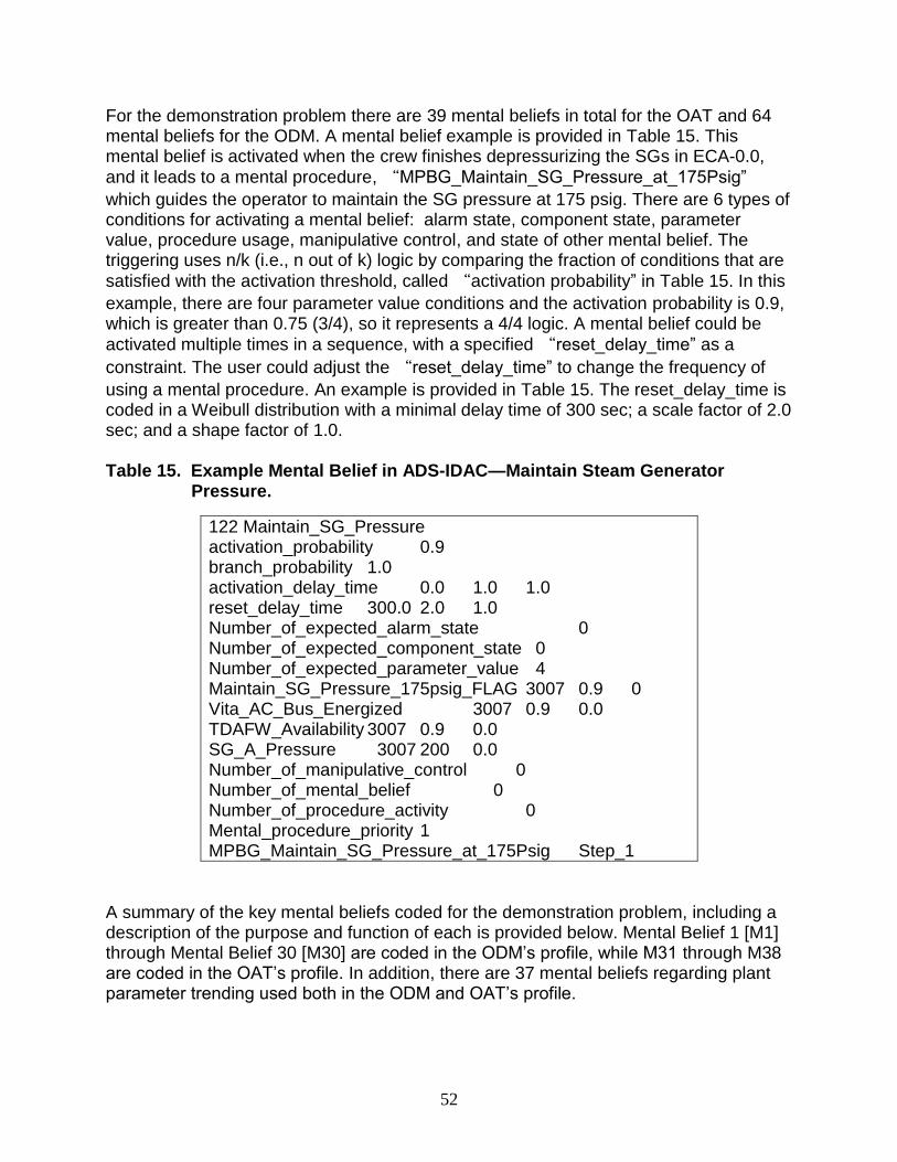
52

For the demonstration problem there are 39 mental beliefs in total for the OAT and 64 mental beliefs for the ODM. A mental belief example is provided in Table 15. This mental belief is activated when the crew finishes depressurizing the SGs in ECA-0.0,

and it leads to a mental procedure, “MPBG_Maintain_SG_Pressure_at_175Psig”

which guides the operator to maintain the SG pressure at 175 psig. There are 6 types of conditions for activating a mental belief: alarm state, component state, parameter value, procedure usage, manipulative control, and state of other mental belief. The triggering uses n/k (i.e., n out of k) logic by comparing the fraction of conditions that are

satisfied with the activation threshold, called “activation probability” in Table 15. In this

example, there are four parameter value conditions and the activation probability is 0.9, which is greater than 0.75 (3/4), so it represents a 4/4 logic. A mental belief could be

activated multiple times in a sequence, with a specified “reset_delay_time” as a

constraint. The user could adjust the “reset_delay_time” to change the frequency of

using a mental procedure. An example is provided in Table 15. The reset_delay_time is coded in a Weibull distribution with a minimal delay time of 300 sec; a scale factor of 2.0 sec; and a shape factor of 1.0. Table 15. Example Mental Belief in ADS-IDAC—Maintain Steam Generator

Pressure.

122 Maintain_SG_Pressure activation_probability 0.9 branch_probability 1.0 activation_delay_time 0.0 1.0 1.0 reset_delay_time 300.0 2.0 1.0 Number_of_expected_alarm_state 0 Number_of_expected_component_state 0 Number_of_expected_parameter_value 4 Maintain_SG_Pressure_175psig_FLAG 3007 0.9 0 Vita_AC_Bus_Energized 3007 0.9 0.0 TDAFW_Availability 3007 0.9 0.0 SG_A_Pressure 3007 200 0.0 Number_of_manipulative_control 0 Number_of_mental_belief 0 Number_of_procedure_activity 0 Mental_procedure_priority 1 MPBG_Maintain_SG_Pressure_at_175Psig Step_1

A summary of the key mental beliefs coded for the demonstration problem, including a description of the purpose and function of each is provided below. Mental Belief 1 [M1] through Mental Belief 30 [M30] are coded in the ODM’s profile, while M31 through M38 are coded in the OAT’s profile. In addition, there are 37 mental beliefs regarding plant parameter trending used both in the ODM and OAT’s profile.

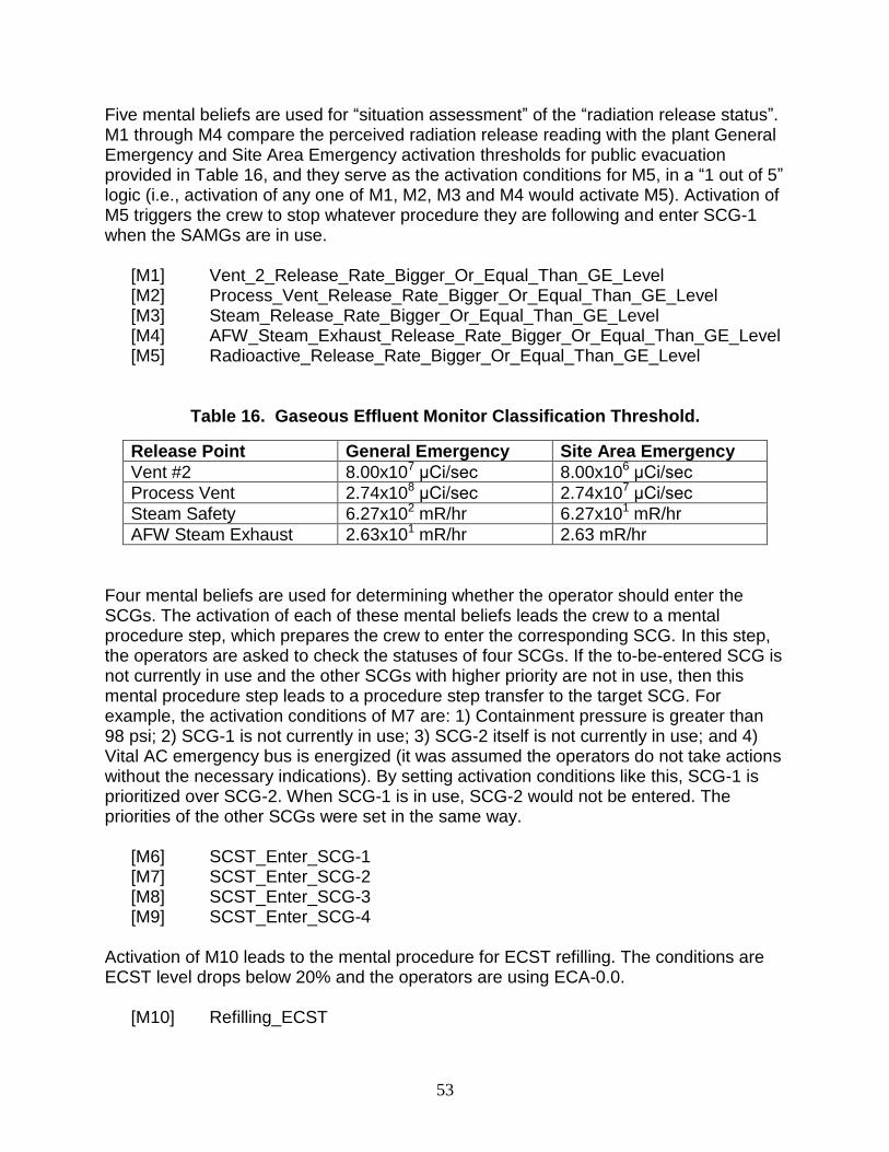
53

Five mental beliefs are used for “situation assessment” of the “radiation release status”. M1 through M4 compare the perceived radiation release reading with the plant General Emergency and Site Area Emergency activation thresholds for public evacuation provided in Table 16, and they serve as the activation conditions for M5, in a “1 out of 5” logic (i.e., activation of any one of M1, M2, M3 and M4 would activate M5). Activation of M5 triggers the crew to stop whatever procedure they are following and enter SCG-1 when the SAMGs are in use.

[M1] Vent_2_Release_Rate_Bigger_Or_Equal_Than_GE_Level [M2] Process_Vent_Release_Rate_Bigger_Or_Equal_Than_GE_Level [M3] Steam_Release_Rate_Bigger_Or_Equal_Than_GE_Level [M4] AFW_Steam_Exhaust_Release_Rate_Bigger_Or_Equal_Than_GE_Level [M5] Radioactive_Release_Rate_Bigger_Or_Equal_Than_GE_Level

Table 16. Gaseous Effluent Monitor Classification Threshold.

Release Point General Emergency Site Area Emergency

Vent #2 8.00x107 μCi/sec 8.00x106 μCi/sec

Process Vent 2.74x108 μCi/sec 2.74x107 μCi/sec

Steam Safety 6.27x102 mR/hr 6.27x101 mR/hr

AFW Steam Exhaust 2.63x101 mR/hr 2.63 mR/hr

Four mental beliefs are used for determining whether the operator should enter the SCGs. The activation of each of these mental beliefs leads the crew to a mental procedure step, which prepares the crew to enter the corresponding SCG. In this step, the operators are asked to check the statuses of four SCGs. If the to-be-entered SCG is not currently in use and the other SCGs with higher priority are not in use, then this mental procedure step leads to a procedure step transfer to the target SCG. For example, the activation conditions of M7 are: 1) Containment pressure is greater than 98 psi; 2) SCG-1 is not currently in use; 3) SCG-2 itself is not currently in use; and 4) Vital AC emergency bus is energized (it was assumed the operators do not take actions without the necessary indications). By setting activation conditions like this, SCG-1 is prioritized over SCG-2. When SCG-1 is in use, SCG-2 would not be entered. The priorities of the other SCGs were set in the same way.

[M6] SCST_Enter_SCG-1 [M7] SCST_Enter_SCG-2 [M8] SCST_Enter_SCG-3 [M9] SCST_Enter_SCG-4

Activation of M10 leads to the mental procedure for ECST refilling. The conditions are ECST level drops below 20% and the operators are using ECA-0.0.

[M10] Refilling_ECST

54

There are four mental beliefs for assessing the hydrogen flammability condition of the containment (M11 through M14). They are used to support the decision on whether to initiate or continue the use of containment spray.

[M11] H2_Severe_Challenge_Zone [M12] Transition_Burn_To_Severe [M13] Transition_Possible_Severe_To_Severe [M14] Containment_Hyrodgen_Unacceptable

Two mental beliefs lead to two mental procedures to simulate the operator following SACRG-2 in parallel with the DFC and SCST (M15 and M16). The reset_delay_time of SACRG2_Scan1 (i.e., frequent monitoring list) is 1800 seconds and the reset_delay_time of SACRG2_Scan2 (i.e., slower monitoring list) is 300 seconds This means the operator would check the indications on the frequent monitoring list every 30 minutes and check the indications on the slower monitoring list every 5 minutes.

[M15] SACRG2_Scan1 [M16] SACRG2_Scan2

One mental belief (M17) is set to be activated when the operator enters ECA-0.0 with a conditional probability of 0.5. In the branch where this mental belief is activated, the operator would depressurize the SGs at cooldown rate of 100 oF/hr while in the other branch, the operator would depressurize the SGs at a slower cooldown rate of 50 oF/hr.

[M17] SG_Depresure_Rate_Full During loss of control panel indications, two mental beliefs (M18 and M19) are activated. They are used to simulate operators looping in ECA-0.0 without doing anything except trying to recover the instrument indications by connecting the portable generator to the vital AC bus. If the loss of indication lasts more than one hour, the operator would transition to the SAMGs.

[M18] ECA_0.0_Looping [M19] ECA_0.0_Transit_To_SAMG

M20 leads the crew to a mental procedure step for connecting the portable generator to the vital AC bus 3 hours after the station blackout with a conditional probability of 0.5. In the branch where the portable generator is assumed not to be connected following DC battery depletion, the operator is assumed to spend one hour to try and connect it to the bus (M21).

[M20] Hardware_Connect_Portable_Generator_at_3Hour [M21] Hardware_Connect_Portable_Generator

55

M22 is activated after the operator finishes depressurizing the SGs to 175 psig. It leads to a mental procedure that guides the operator to use the SG PORVs to maintain the SGs pressure around 175 psig.

[M22] Maintain_SG_Pressure M23 through M26 are used for the diagnosis of a SGTR (a SGTR was not included in the sample problem). The activation conditions for M23, M24, and M25 are the SG level deviating from the set point (higher) and increasing with the level increase not caused by AFW over feeding but as a result of a SGTR.

[M23] SG_A_Uncontrolled_Level_Increase [M24] SG_B_Uncontrolled_Level_Increase [M25] SG_C_Uncontrolled_Level_Increase [M26] SG_Uncontrolled_Level_Increase

M27 and M28 are work-arounds for generating hardware event branching.

[M27] Hardware_RCP_Leakage [M28] Hardware_Battery_Depletion

M29 activates a mental procedure step repeatedly to check indications (e.g. battery status), in order to make sure some important plant state changes are captured by the mental process and activate relevant mental beliefs.

[M29] Constant_Scan M30 is active when the reactor trips. It guides the operator to enter the written

procedure step which is listed as the first one in the “Procedures.txt” input (i.e.,

normally the first procedural step would be E-0, Step 1).

[M30] Reactor_Tripped M31 through M38 are used for the operator to control the TDAFW flow to maintain the SG levels. After reactor trip, M31 guides the operator to a mental procedure to maximize TDAFW pump flow. Then M33 through M38 guide the operator with two mental procedures to adjust the flow by a step change of the valve position when the SG level is too high or too low.

[M31] Align_TDAFP_Flow_Path [M32] TDAFP_Flowpath_Aligned [M33] SG_A_Reduce_TDAFW [M34] SG_A_Increase_TDAFW [M35] SG_B_Reduce_TDAFW [M36] SG_B_Increase_TDAFW [M37] SG_C_Reduce_TDAFW

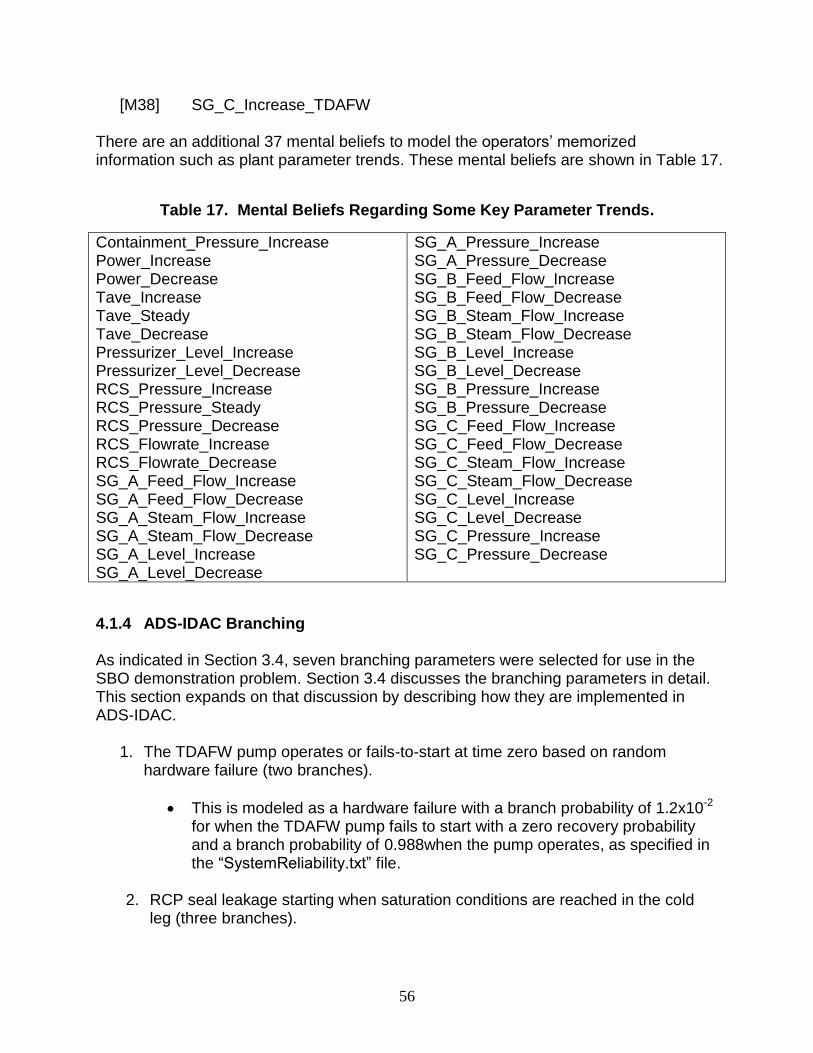
56

[M38] SG_C_Increase_TDAFW There are an additional 37 mental beliefs to model the operators’ memorized information such as plant parameter trends. These mental beliefs are shown in Table 17.

Table 17. Mental Beliefs Regarding Some Key Parameter Trends.

Containment_Pressure_Increase Power_Increase Power_Decrease Tave_Increase Tave_Steady Tave_Decrease Pressurizer_Level_Increase Pressurizer_Level_Decrease RCS_Pressure_Increase RCS_Pressure_Steady RCS_Pressure_Decrease RCS_Flowrate_Increase RCS_Flowrate_Decrease SG_A_Feed_Flow_Increase SG_A_Feed_Flow_Decrease SG_A_Steam_Flow_Increase SG_A_Steam_Flow_Decrease SG_A_Level_Increase SG_A_Level_Decrease

SG_A_Pressure_Increase SG_A_Pressure_Decrease SG_B_Feed_Flow_Increase SG_B_Feed_Flow_Decrease SG_B_Steam_Flow_Increase SG_B_Steam_Flow_Decrease SG_B_Level_Increase SG_B_Level_Decrease SG_B_Pressure_Increase SG_B_Pressure_Decrease SG_C_Feed_Flow_Increase SG_C_Feed_Flow_Decrease SG_C_Steam_Flow_Increase SG_C_Steam_Flow_Decrease SG_C_Level_Increase SG_C_Level_Decrease SG_C_Pressure_Increase SG_C_Pressure_Decrease

4.1.4 ADS-IDAC Branching As indicated in Section 3.4, seven branching parameters were selected for use in the SBO demonstration problem. Section 3.4 discusses the branching parameters in detail. This section expands on that discussion by describing how they are implemented in ADS-IDAC.

1. The TDAFW pump operates or fails-to-start at time zero based on random hardware failure (two branches).

This is modeled as a hardware failure with a branch probability of 1.2x10-2 for when the TDAFW pump fails to start with a zero recovery probability and a branch probability of 0.988when the pump operates, as specified in the “SystemReliability.txt” file.

2. RCP seal leakage starting when saturation conditions are reached in the cold

leg (three branches).

57

The default seal leakage rate is set to be 21 gpm per pump at time zero. A mental procedure is created to have the operator constantly monitor the RCP seal saturation status. Once the RCP control volume in MELCOR reaches saturation, a mental belief is activated and triggers a mental procedure to send an order to MELCOR to the appropriate leak rate. Three branches are generated with three different leakage rates: (a) 21 gpm per pump with conditional probability of 0.80, (b) 182 gpm per pump with conditional probability of 0.1975, or (c) 480 gpm per pump with conditional probability of 0.0025.

3. Rate of depressurization of the SGs in ECA-0.0, if the TDAFW pump is available (two branches).

This branching is set up in a mental belief. If the TDAFW pump is available, a mental belief “SG_Depresure_Rate_Full” [M17] is activated with a conditional probability of 0.8. When the operators proceed to the RCS depressurization step in ECA-0.0 and, if this mental belief is activated, a cooldown rate of 100 oF/hr is used, otherwise a slower cooldown rate of 50 oF/hr is used.

4. Time of DC battery depletion (distribution –three branches)

This is realized by a mental belief and mental procedure step. The action delay time is generated three times for the DC battery depletion. These times are means of three equal probability segments of a Weibull CDF used to model the uncertainty in battery depletion time. Using Equation 1, and the variable inputs below, the means of the three equal probability segments were calculated. This is another work around where a human model channel is used to generate hardware failure branches. µ= 7200 (sec) α = 12114.72 (sec) β = 2.6527

5. Restoration of power to a vital AC bus for critical instrumentation at a specified time (binary branch).

This is realized by using one initiating event, one mental belief, and one mental procedure. This initiating event connects the generator to a vital AC bus at 3 hours with a conditional probability of 0.5. If the AC vital bus is not energized when DC batteries are depleted, the mental belief will trigger a mental procedure step one hour later to connect the portable generator to the vital AC bus.

58

6. Core degradation assumptions related to the fuel failure criterion: Zircaloy metal breakout temperature, molten clad draining rate, and radial debris relocation time constants (three branches).

This is done by running three separate simulations for both a STSBO and a LTSBO scenario using three different MELCOR input models.

7. Time delays for connecting the portable diesel-driven Godwin pump for either containment spray injection or refilling the ECST (distribution – three branches).

Branches for ECST refilling are generated from a mental belief. Branches for containment spray are generated in three relevant procedure steps. A Weibull distribution in Equation 1 with the following parameters is used for this parameter: µ = 0 (sec) α = 8684.044 (sec) β = 3.0139

4.1.5 Crew Variation and Limited Indication Effect Captured in the Demonstration Simulation Some potential crew-to-crew variations are captured in the demonstration problem by varying the following action parameters:

Time variations of actions to connect the portable generator to the vital AC bus and to prepare the Godwin pump for ECST refill or containment spray.

RCS depressurization rate.

Two types of limited indications are modeled. First, to measure the containment hydrogen percent, the operators need to take samples and analyze them. It is assumed that it would take 30 minutes to get a hydrogen percentage reading. Therefore, the SACRG-2 guideline is coded in such a way that containment hydrogen percentage is read once every 30 minutes while the other parameters are scanned more frequently. When making decision on whether to initiate the containment spray, the operators use the last reading of the value of hydrogen percentage, which might not actually reflect the actual hydrogen level. Second, it is possible that the DC batteries deplete before the portable generator gets connected. In this case, the crew loses all indications. In the ADS-IDAC input, the operators are informed to loop through the DFC procedure until indicators are recovered.

4.2 ADS Modifications In the demonstration problem, there are three major concerns for the operators: fission product release, over-pressurization of the containment, and a hydrogen deflagration.

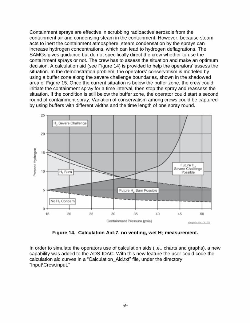
59

Containment sprays are effective in scrubbing radioactive aerosols from the containment air and condensing steam in the containment. However, because steam acts to inert the containment atmosphere, steam condensation by the sprays can increase hydrogen concentrations, which can lead to hydrogen deflagrations. The SAMGs gives guidance but do not specifically direct the crew whether to use the containment sprays or not. The crew has to assess the situation and make an optimum decision. A calculation aid (see Figure 14) is provided to help the operators’ assess the situation. In the demonstration problem, the operators’ conservatism is modeled by using a buffer zone along the severe challenge boundaries, shown in the shadowed area of Figure 15. Once the current situation is below the buffer zone, the crew could initiate the containment spray for a time interval, then stop the spray and reassess the situation. If the condition is still below the buffer zone, the operator could start a second round of containment spray. Variation of conservatism among crews could be captured by using buffers with different widths and the time length of one spray round.

Figure 14. Calculation Aid-7, no venting, wet H2 measurement.

In order to simulate the operators use of calculation aids (i.e., charts and graphs), a new capability was added to the ADS-IDAC. With this new feature the user could code the calculation aid curves in a “Calculation_Aid.txt” file, under the directory “Input\Crew.input.”

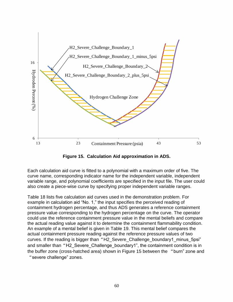
60

Figure 15. Calculation Aid approximation in ADS.

Each calculation aid curve is fitted to a polynomial with a maximum order of five. The curve name, corresponding indicator name for the independent variable, independent variable range, and polynomial coefficients are specified in the input file. The user could also create a piece-wise curve by specifying proper independent variable ranges. Table 18 lists five calculation aid curves used in the demonstration problem. For example in calculation aid “No. 1,” the input specifies the perceived reading of containment hydrogen percentage, and thus ADS generates a reference containment pressure value corresponding to the hydrogen percentage on the curve. The operator could use the reference containment pressure value in the mental beliefs and compare the actual reading value against it to determine the containment flammability condition. An example of a mental belief is given in Table 19. This mental belief compares the actual containment pressure reading against the reference pressure values of two

curves. If the reading is bigger than“H2_Severe_Challenge_boundary1_minus_5psi”

and smaller than“H2_Severe_Challenge_boundary1”, the containment condition is in

the buffer zone (cross-hatched area) shown in Figure 15 between the “burn” zone and

“severe challenge” zones.

6

16

13 23 33 43 53Containment Pressure (psia)

Hy

dro

den

Perce

nt (%

)

Hydrogen Challenge Zone

H2_Severe_Challenge_Boundary_1

H2_Severe_Challenge_Boundary_1_minus_5psi

H2_Severe_Challenge_Boundary_2

H2_Severe_Challenge_Boundary_2_plus_5psi

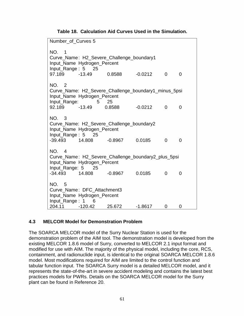
61

Table 18. Calculation Aid Curves Used in the Simulation.

Number_of_Curves 5 NO. 1 Curve_Name : H2_Severe_Challenge_boundary1 Input_Name Hydrogen_Percent Input_Range : 5 25 97.189 -13.49 0.8588 -0.0212 0 0 NO. 2 Curve_Name: H2_Severe_Challenge_boundary1_minus_5psi Input_Name Hydrogen_Percent Input_Range: 5 25 92.189 -13.49 0.8588 -0.0212 0 0 NO. 3 Curve_Name: H2_Severe_Challenge_boundary2 Input_Name Hydrogen_Percent Input_Range : 5 25 -39.493 14.808 -0.8967 0.0185 0 0 NO. 4 Curve_Name : H2_Severe_Challenge_boundary2_plus_5psi Input_Name Hydrogen_Percent Input_Range: 5 25 -34.493 14.808 -0.8967 0.0185 0 0 NO. 5 Curve_Name : DFC_Attachment3 Input_Name Hydrogen_Percent Input_Range : 1 6 204.11 -120.42 25.672 -1.8617 0 0

4.3 MELCOR Model for Demonstration Problem The SOARCA MELCOR model of the Surry Nuclear Station is used for the demonstration problem of the AIM tool. The demonstration model is developed from the existing MELCOR 1.8.6 model of Surry, converted to MELCOR 2.1 input format and modified for use with AIM. The majority of the physical model, including the core, RCS, containment, and radionuclide input, is identical to the original SOARCA MELCOR 1.8.6 model. Most modifications required for AIM are limited to the control function and tabular function input. The SOARCA Surry model is a detailed MELCOR model, and it represents the state-of-the-art in severe accident modeling and contains the latest best practices models for PWRs. Details on the SOARCA MELCOR model for the Surry plant can be found in Reference 20.

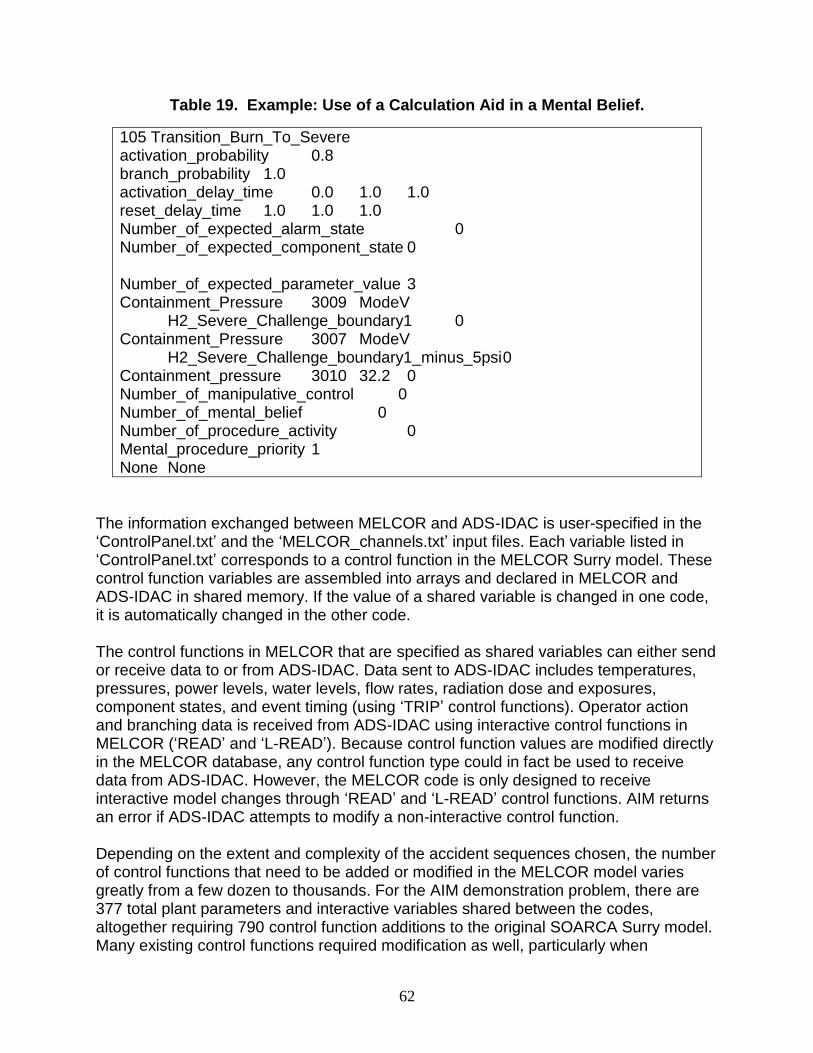
62

Table 19. Example: Use of a Calculation Aid in a Mental Belief.

105 Transition_Burn_To_Severe activation_probability 0.8 branch_probability 1.0 activation_delay_time 0.0 1.0 1.0 reset_delay_time 1.0 1.0 1.0 Number_of_expected_alarm_state 0 Number_of_expected_component_state 0 Number_of_expected_parameter_value 3 Containment_Pressure 3009 ModeV H2_Severe_Challenge_boundary1 0 Containment_Pressure 3007 ModeV H2_Severe_Challenge_boundary1_minus_5psi 0 Containment_pressure 3010 32.2 0 Number_of_manipulative_control 0 Number_of_mental_belief 0 Number_of_procedure_activity 0 Mental_procedure_priority 1 None None

The information exchanged between MELCOR and ADS-IDAC is user-specified in the ‘ControlPanel.txt’ and the ‘MELCOR_channels.txt’ input files. Each variable listed in ‘ControlPanel.txt’ corresponds to a control function in the MELCOR Surry model. These control function variables are assembled into arrays and declared in MELCOR and ADS-IDAC in shared memory. If the value of a shared variable is changed in one code, it is automatically changed in the other code. The control functions in MELCOR that are specified as shared variables can either send or receive data to or from ADS-IDAC. Data sent to ADS-IDAC includes temperatures, pressures, power levels, water levels, flow rates, radiation dose and exposures, component states, and event timing (using ‘TRIP’ control functions). Operator action and branching data is received from ADS-IDAC using interactive control functions in MELCOR (‘READ’ and ‘L-READ’). Because control function values are modified directly in the MELCOR database, any control function type could in fact be used to receive data from ADS-IDAC. However, the MELCOR code is only designed to receive interactive model changes through ‘READ’ and ‘L-READ’ control functions. AIM returns an error if ADS-IDAC attempts to modify a non-interactive control function. Depending on the extent and complexity of the accident sequences chosen, the number of control functions that need to be added or modified in the MELCOR model varies greatly from a few dozen to thousands. For the AIM demonstration problem, there are 377 total plant parameters and interactive variables shared between the codes, altogether requiring 790 control function additions to the original SOARCA Surry model. Many existing control functions required modification as well, particularly when

63

automatic or assumed operator actions needed to be removed from the MELCOR model. Several tabular functions are also added to the SOARCA Surry model that supports operator actions such as TDAFW pump throttling and the cooldown rate of the steam generators, which is a branching parameter for this study.

The modifications to the SOARCA Surry model allow the following variables to be available for interactive manipulation by ADS-IDAC:

1. SG PORVs – operators can control the valve positions, or set the PORVs in “automatic” mode.

2. TDAFW pump discharge valve positions – allows operators to throttle TDAFW injection to maintain nominal SG water levels.

3. Steam dump valves to TDAFW pump – operators can close to terminate TDAFW injection.

4. Containment sprays – operators determine when to activate containment sprays using a Godwin pump (branching parameter).

5. ECST refill – operators can use the Godwin pump to refill the ECST if TDAFW is available (branching parameter).

6. TDAFW pump availability – allows ADS-IDAC to interactively select which sequences have the TDAFW pump being defined as available (branching parameter).

7. Battery depletion time – ADS-IDAC can interactively determine the time at which DC battery power will terminate (branching parameter).

8. RCP seal leakage rate upon saturation – ADS-IDAC can determine the leakage rate from the RCP seals (branching parameter).

9. SG cooldown rate – ADS-IDAC can determine the rate of the SG depressurization by manipulating the valve positions on the SG PORV (branching parameter).

Many other additional control function modifications were made to the SOARCA Surry model in order to facilitate additional interaction with ADS-IDAC, but they are not necessary for the STSBO and LTSBO accident scenarios selected for this work. Table 20 provides a detailed list of major plant variables that MELCOR sends to ADS-IDAC every ΔtADS time interval. Also listed in Table 20 are the control functions corresponding to each plant variable, along with the units of the variable (if applicable). Most of the plant variables in Table 20 are used in the procedures input files for the demonstration problem; others are carry-overs from an earlier Beaver Valley problem analyzed by ADS-IDAC/RELAP5 [18].

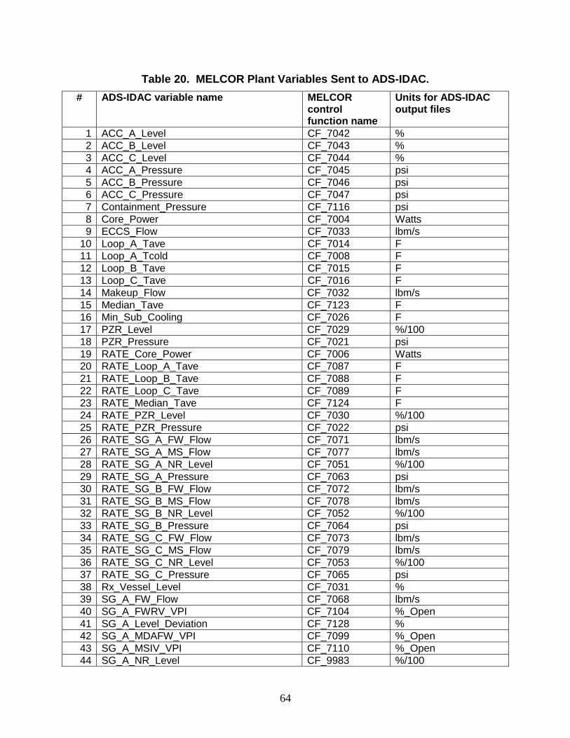
64

Table 20. MELCOR Plant Variables Sent to ADS-IDAC.

# ADS-IDAC variable name MELCOR control function name

Units for ADS-IDAC output files

1 ACC_A_Level CF_7042 %

2 ACC_B_Level CF_7043 %

3 ACC_C_Level CF_7044 %

4 ACC_A_Pressure CF_7045 psi

5 ACC_B_Pressure CF_7046 psi

6 ACC_C_Pressure CF_7047 psi

7 Containment_Pressure CF_7116 psi

8 Core_Power CF_7004 Watts

9 ECCS_Flow CF_7033 lbm/s

10 Loop_A_Tave CF_7014 F

11 Loop_A_Tcold CF_7008 F

12 Loop_B_Tave CF_7015 F

13 Loop_C_Tave CF_7016 F

14 Makeup_Flow CF_7032 lbm/s

15 Median_Tave CF_7123 F

16 Min_Sub_Cooling CF_7026 F

17 PZR_Level CF_7029 %/100

18 PZR_Pressure CF_7021 psi

19 RATE_Core_Power CF_7006 Watts

20 RATE_Loop_A_Tave CF_7087 F

21 RATE_Loop_B_Tave CF_7088 F

22 RATE_Loop_C_Tave CF_7089 F

23 RATE_Median_Tave CF_7124 F

24 RATE_PZR_Level CF_7030 %/100

25 RATE_PZR_Pressure CF_7022 psi

26 RATE_SG_A_FW_Flow CF_7071 lbm/s

27 RATE_SG_A_MS_Flow CF_7077 lbm/s

28 RATE_SG_A_NR_Level CF_7051 %/100

29 RATE_SG_A_Pressure CF_7063 psi

30 RATE_SG_B_FW_Flow CF_7072 lbm/s

31 RATE_SG_B_MS_Flow CF_7078 lbm/s

32 RATE_SG_B_NR_Level CF_7052 %/100

33 RATE_SG_B_Pressure CF_7064 psi

34 RATE_SG_C_FW_Flow CF_7073 lbm/s

35 RATE_SG_C_MS_Flow CF_7079 lbm/s

36 RATE_SG_C_NR_Level CF_7053 %/100

37 RATE_SG_C_Pressure CF_7065 psi

38 Rx_Vessel_Level CF_7031 %

39 SG_A_FW_Flow CF_7068 lbm/s

40 SG_A_FWRV_VPI CF_7104 %_Open

41 SG_A_Level_Deviation CF_7128 %

42 SG_A_MDAFW_VPI CF_7099 %_Open

43 SG_A_MSIV_VPI CF_7110 %_Open

44 SG_A_NR_Level CF_9983 %/100

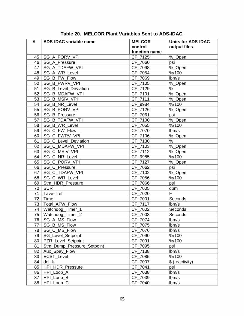
65




45 SG_A_PORV_VPI CF_7125 %_Open

46 SG_A_Pressure CF_7060 psi

47 SG_A_TDAFW_VPI CF_7098 %_Open

48 SG_A_WR_Level CF_7054 %/100

49 SG_B_FW_Flow CF_7069 lbm/s

50 SG_B_FWRV_VPI CF_7105 %_Open

51 SG_B_Level_Deviation CF_7129 %

52 SG_B_MDAFW_VPI CF_7101 %_Open

53 SG_B_MSIV_VPI CF_7111 %_Open

54 SG_B_NR_Level CF_9984 %/100

55 SG_B_PORV_VPI CF_7126 %_Open

56 SG_B_Pressure CF_7061 psi

57 SG_B_TDAFW_VPI CF_7100 %_Open

58 SG_B_WR_Level CF_7055 %/100

59 SG_C_FW_Flow CF_7070 lbm/s

60 SG_C_FWRV_VPI CF_7106 %_Open

61 SG_C_Level_Deviation CF_7130 %

62 SG_C_MDAFW_VPI CF_7103 %_Open

63 SG_C_MSIV_VPI CF_7112 %_Open

64 SG_C_NR_Level CF_9985 %/100

65 SG_C_PORV_VPI CF_7127 %_Open

66 SG_C_Pressure CF_7062 psi

67 SG_C_TDAFW_VPI CF_7102 %_Open

68 SG_C_WR_Level CF_7056 %/100

69 Stm_HDR_Pressure CF_7066 psi

70 SUR CF_7005 dpm

71 Tave-Tref CF_7020 F

72 Time CF_7001 Seconds

73 Total_AFW_Flow CF_7117 lbm/s

74 Watchdog_Timer_1 CF_7002 Seconds

75 Watchdog_Timer_2 CF_7003 Seconds

76 SG_A_MS_Flow CF_7074 lbm/s

77 SG_B_MS_Flow CF_7075 lbm/s

78 SG_C_MS_Flow CF_7076 lbm/s

79 SG_Level_Setpoint CF_7090 %/100

80 PZR_Level_Setpoint CF_7091 %/100

81 Stm_Dump_Pressure_Setpoint CF_7095 psi

82 Aux_Spay_Flow CF_7138 lbm/s

83 ECST_Level CF_7085 %/100

84 del_k CF_7007 $ (reactivity)

85 HPI_HDR_Pressure CF_7041 psi

86 HPI_Loop_A CF_7038 lbm/s

87 HPI_Loop_B CF_7039 lbm/s

88 HPI_Loop_C CF_7040 lbm/s

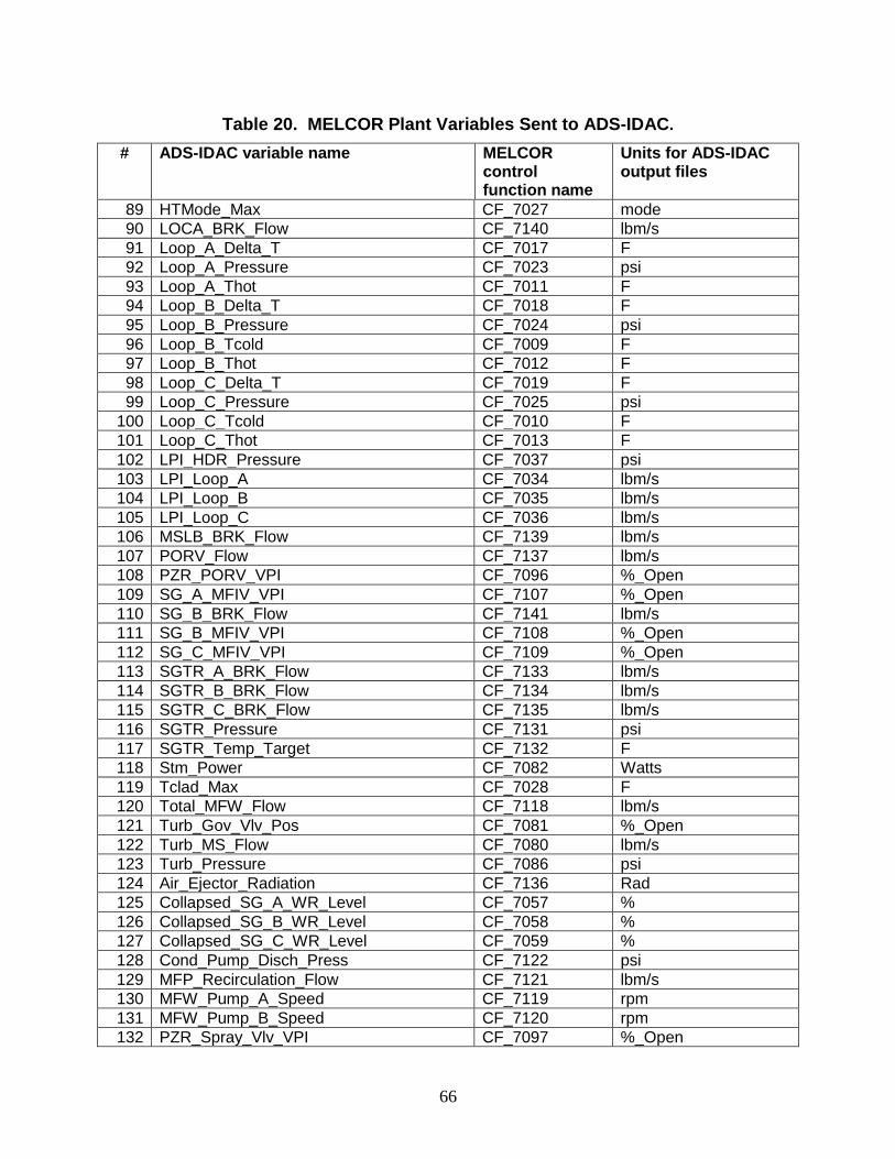
66




89 HTMode_Max CF_7027 mode

90 LOCA_BRK_Flow CF_7140 lbm/s

91 Loop_A_Delta_T CF_7017 F

92 Loop_A_Pressure CF_7023 psi

93 Loop_A_Thot CF_7011 F

94 Loop_B_Delta_T CF_7018 F

95 Loop_B_Pressure CF_7024 psi

96 Loop_B_Tcold CF_7009 F

97 Loop_B_Thot CF_7012 F

98 Loop_C_Delta_T CF_7019 F

99 Loop_C_Pressure CF_7025 psi

100 Loop_C_Tcold CF_7010 F

101 Loop_C_Thot CF_7013 F

102 LPI_HDR_Pressure CF_7037 psi

103 LPI_Loop_A CF_7034 lbm/s

104 LPI_Loop_B CF_7035 lbm/s

105 LPI_Loop_C CF_7036 lbm/s

106 MSLB_BRK_Flow CF_7139 lbm/s

107 PORV_Flow CF_7137 lbm/s

108 PZR_PORV_VPI CF_7096 %_Open

109 SG_A_MFIV_VPI CF_7107 %_Open

110 SG_B_BRK_Flow CF_7141 lbm/s

111 SG_B_MFIV_VPI CF_7108 %_Open

112 SG_C_MFIV_VPI CF_7109 %_Open

113 SGTR_A_BRK_Flow CF_7133 lbm/s

114 SGTR_B_BRK_Flow CF_7134 lbm/s

115 SGTR_C_BRK_Flow CF_7135 lbm/s

116 SGTR_Pressure CF_7131 psi

117 SGTR_Temp_Target CF_7132 F

118 Stm_Power CF_7082 Watts

119 Tclad_Max CF_7028 F

120 Total_MFW_Flow CF_7118 lbm/s

121 Turb_Gov_Vlv_Pos CF_7081 %_Open

122 Turb_MS_Flow CF_7080 lbm/s

123 Turb_Pressure CF_7086 psi

124 Air_Ejector_Radiation CF_7136 Rad

125 Collapsed_SG_A_WR_Level CF_7057 %

126 Collapsed_SG_B_WR_Level CF_7058 %

127 Collapsed_SG_C_WR_Level CF_7059 %

128 Cond_Pump_Disch_Press CF_7122 psi

129 MFP_Recirculation_Flow CF_7121 lbm/s

130 MFW_Pump_A_Speed CF_7119 rpm

131 MFW_Pump_B_Speed CF_7120 rpm

132 PZR_Spray_Vlv_VPI CF_7097 %_Open

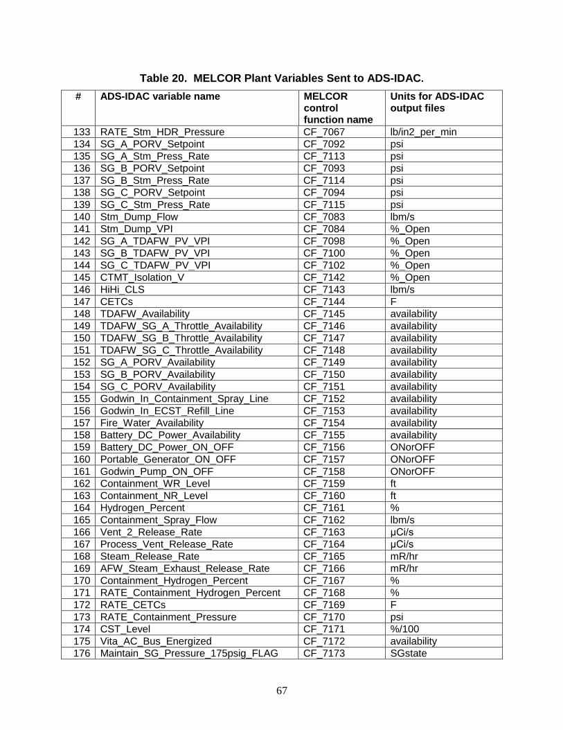
67




133 RATE_Stm_HDR_Pressure CF_7067 lb/in2_per_min

134 SG_A_PORV_Setpoint CF_7092 psi

135 SG_A_Stm_Press_Rate CF_7113 psi

136 SG_B_PORV_Setpoint CF_7093 psi

137 SG_B_Stm_Press_Rate CF_7114 psi

138 SG_C_PORV_Setpoint CF_7094 psi

139 SG_C_Stm_Press_Rate CF_7115 psi

140 Stm_Dump_Flow CF_7083 lbm/s

141 Stm_Dump_VPI CF_7084 %_Open

142 SG_A_TDAFW_PV_VPI CF_7098 %_Open

143 SG_B_TDAFW_PV_VPI CF_7100 %_Open

144 SG_C_TDAFW_PV_VPI CF_7102 %_Open

145 CTMT_Isolation_V CF_7142 %_Open

146 HiHi_CLS CF_7143 lbm/s

147 CETCs CF_7144 F

148 TDAFW_Availability CF_7145 availability

149 TDAFW_SG_A_Throttle_Availability CF_7146 availability

150 TDAFW_SG_B_Throttle_Availability CF_7147 availability

151 TDAFW_SG_C_Throttle_Availability CF_7148 availability

152 SG_A_PORV_Availability CF_7149 availability

153 SG_B_PORV_Availability CF_7150 availability

154 SG_C_PORV_Availability CF_7151 availability

155 Godwin_In_Containment_Spray_Line CF_7152 availability

156 Godwin_In_ECST_Refill_Line CF_7153 availability

157 Fire_Water_Availability CF_7154 availability

158 Battery_DC_Power_Availability CF_7155 availability

159 Battery_DC_Power_ON_OFF CF_7156 ONorOFF

160 Portable_Generator_ON_OFF CF_7157 ONorOFF

161 Godwin_Pump_ON_OFF CF_7158 ONorOFF

162 Containment_WR_Level CF_7159 ft

163 Containment_NR_Level CF_7160 ft

164 Hydrogen_Percent CF_7161 %

165 Containment_Spray_Flow CF_7162 lbm/s

166 Vent_2_Release_Rate CF_7163 μCi/s

167 Process_Vent_Release_Rate CF_7164 μCi/s

168 Steam_Release_Rate CF_7165 mR/hr

169 AFW_Steam_Exhaust_Release_Rate CF_7166 mR/hr

170 Containment_Hydrogen_Percent CF_7167 %

171 RATE_Containment_Hydrogen_Percent CF_7168 %

172 RATE_CETCs CF_7169 F

173 RATE_Containment_Pressure CF_7170 psi

174 CST_Level CF_7171 %/100

175 Vita_AC_Bus_Energized CF_7172 availability

176 Maintain_SG_Pressure_175psig_FLAG CF_7173 SGstate

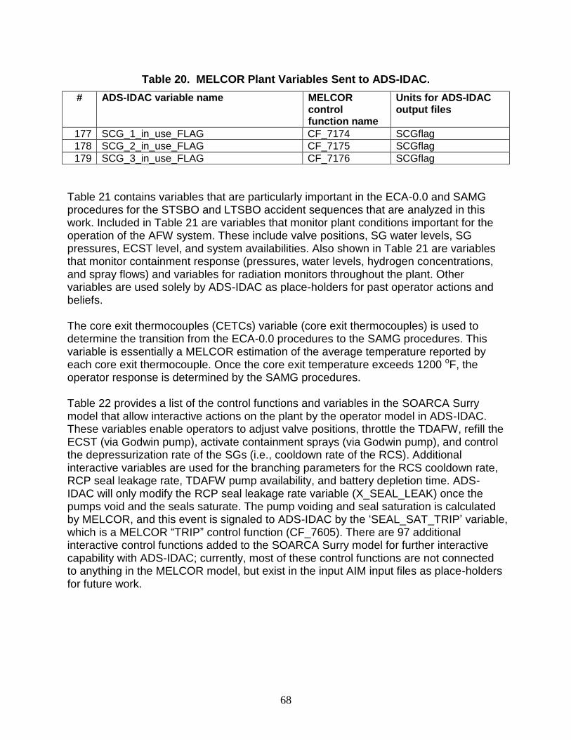
68




177 SCG_1_in_use_FLAG CF_7174 SCGflag



Table 21 contains variables that are particularly important in the ECA-0.0 and SAMG procedures for the STSBO and LTSBO accident sequences that are analyzed in this work. Included in Table 21 are variables that monitor plant conditions important for the operation of the AFW system. These include valve positions, SG water levels, SG pressures, ECST level, and system availabilities. Also shown in Table 21 are variables that monitor containment response (pressures, water levels, hydrogen concentrations, and spray flows) and variables for radiation monitors throughout the plant. Other variables are used solely by ADS-IDAC as place-holders for past operator actions and beliefs. The core exit thermocouples (CETCs) variable (core exit thermocouples) is used to determine the transition from the ECA-0.0 procedures to the SAMG procedures. This variable is essentially a MELCOR estimation of the average temperature reported by each core exit thermocouple. Once the core exit temperature exceeds 1200 oF, the operator response is determined by the SAMG procedures. Table 22 provides a list of the control functions and variables in the SOARCA Surry model that allow interactive actions on the plant by the operator model in ADS-IDAC. These variables enable operators to adjust valve positions, throttle the TDAFW, refill the ECST (via Godwin pump), activate containment sprays (via Godwin pump), and control the depressurization rate of the SGs (i.e., cooldown rate of the RCS). Additional interactive variables are used for the branching parameters for the RCS cooldown rate, RCP seal leakage rate, TDAFW pump availability, and battery depletion time. ADS-IDAC will only modify the RCP seal leakage rate variable (X_SEAL_LEAK) once the pumps void and the seals saturate. The pump voiding and seal saturation is calculated by MELCOR, and this event is signaled to ADS-IDAC by the ‘SEAL_SAT_TRIP’ variable, which is a MELCOR “TRIP” control function (CF_7605). There are 97 additional interactive control functions added to the SOARCA Surry model for further interactive capability with ADS-IDAC; currently, most of these control functions are not connected to anything in the MELCOR model, but exist in the input AIM input files as place-holders for future work.

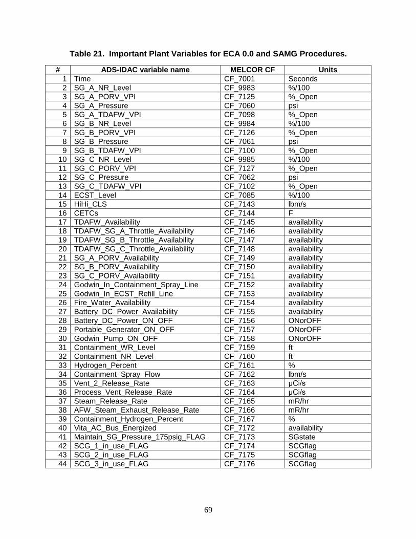
69

Table 21. Important Plant Variables for ECA 0.0 and SAMG Procedures.

# ADS-IDAC variable name MELCOR CF Units

1 Time CF_7001 Seconds

2 SG_A_NR_Level CF_9983 %/100

3 SG_A_PORV_VPI CF_7125 %_Open

4 SG_A_Pressure CF_7060 psi

5 SG_A_TDAFW_VPI CF_7098 %_Open

6 SG_B_NR_Level CF_9984 %/100

7 SG_B_PORV_VPI CF_7126 %_Open

8 SG_B_Pressure CF_7061 psi

9 SG_B_TDAFW_VPI CF_7100 %_Open

10 SG_C_NR_Level CF_9985 %/100

11 SG_C_PORV_VPI CF_7127 %_Open

12 SG_C_Pressure CF_7062 psi

13 SG_C_TDAFW_VPI CF_7102 %_Open

14 ECST_Level CF_7085 %/100

15 HiHi_CLS CF_7143 lbm/s

16 CETCs CF_7144 F

17 TDAFW_Availability CF_7145 availability

18 TDAFW_SG_A_Throttle_Availability CF_7146 availability

19 TDAFW_SG_B_Throttle_Availability CF_7147 availability

20 TDAFW_SG_C_Throttle_Availability CF_7148 availability

21 SG_A_PORV_Availability CF_7149 availability

22 SG_B_PORV_Availability CF_7150 availability

23 SG_C_PORV_Availability CF_7151 availability

24 Godwin_In_Containment_Spray_Line CF_7152 availability

25 Godwin_In_ECST_Refill_Line CF_7153 availability

26 Fire_Water_Availability CF_7154 availability

27 Battery_DC_Power_Availability CF_7155 availability

28 Battery_DC_Power_ON_OFF CF_7156 ONorOFF

29 Portable_Generator_ON_OFF CF_7157 ONorOFF

30 Godwin_Pump_ON_OFF CF_7158 ONorOFF

31 Containment_WR_Level CF_7159 ft

32 Containment_NR_Level CF_7160 ft

33 Hydrogen_Percent CF_7161 %

34 Containment_Spray_Flow CF_7162 lbm/s

35 Vent_2_Release_Rate CF_7163 μCi/s

36 Process_Vent_Release_Rate CF_7164 μCi/s

37 Steam_Release_Rate CF_7165 mR/hr

38 AFW_Steam_Exhaust_Release_Rate CF_7166 mR/hr

39 Containment_Hydrogen_Percent CF_7167 %

40 Vita_AC_Bus_Energized CF_7172 availability

41 Maintain_SG_Pressure_175psig_FLAG CF_7173 SGstate




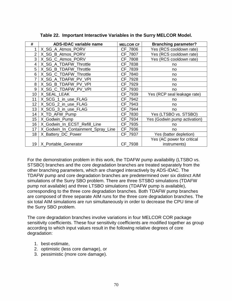
70

Table 22. Important Interactive Variables in the Surry MELCOR Model.

# ADS-IDAC variable name MELCOR CF Branching parameter?

1 X_SG_A_Atmos_PORV CF_7806 Yes (RCS cooldown rate)

2 X_SG_B_Atmos_PORV CF_7807 Yes (RCS cooldown rate)

3 X_SG_C_Atmos_PORV CF_7808 Yes (RCS cooldown rate)

4 X_SG_A_TDAFW_Throttle CF_7838 no

5 X_SG_B_TDAFW_Throttle CF_7839 no

6 X_SG_C_TDAFW_Throttle CF_7840 no

7 X_SG_A_TDAFW_PV_VPI CF_7928 no

8 X_SG_B_TDAFW_PV_VPI CF_7929 no

9 X_SG_C_TDAFW_PV_VPI CF_7930 no

10 X_SEAL_LEAK CF_7939 Yes (RCP seal leakage rate)

11 X_SCG_1_in_use_FLAG CF_7942 no



14 X_TD_AFW_Pump CF_7830 Yes (LTSBO vs. STSBO)

15 X_Godwin_Pump CF_7934 Yes (Godwin pump activation)

16 X_Godwin_In_ECST_Refill_Line CF_7935 no

17 X_Godwin_In_Containment_Spray_Line CF_7936 no

18 X_Battery_DC_Power CF_7937 Yes (batter depletion)

19 X_Portable_Generator CF_7938 Yes (AC power for critical

instruments)

For the demonstration problem in this work, the TDAFW pump availability (LTSBO vs. STSBO) branches and the core degradation branches are treated separately from the other branching parameters, which are changed interactively by ADS-IDAC. The TDAFW pump and core degradation branches are predetermined over six distinct AIM simulations of the Surry SBO problem. There are three STSBO simulations (TDAFW pump not available) and three LTSBO simulations (TDAFW pump is available), corresponding to the three core degradation branches. Both TDAFW pump branches are composed of three separate AIM runs for the three core degradation branches. The six total AIM simulations are run simultaneously in order to decrease the CPU time of the Surry SBO problem. The core degradation branches involve variations in four MELCOR COR package sensitivity coefficients. These four sensitivity coefficients are modified together as group according to which input values result in the following relative degrees of core degradation:

1. best-estimate, 2. optimistic (less core damage), or 3. pessimistic (more core damage).

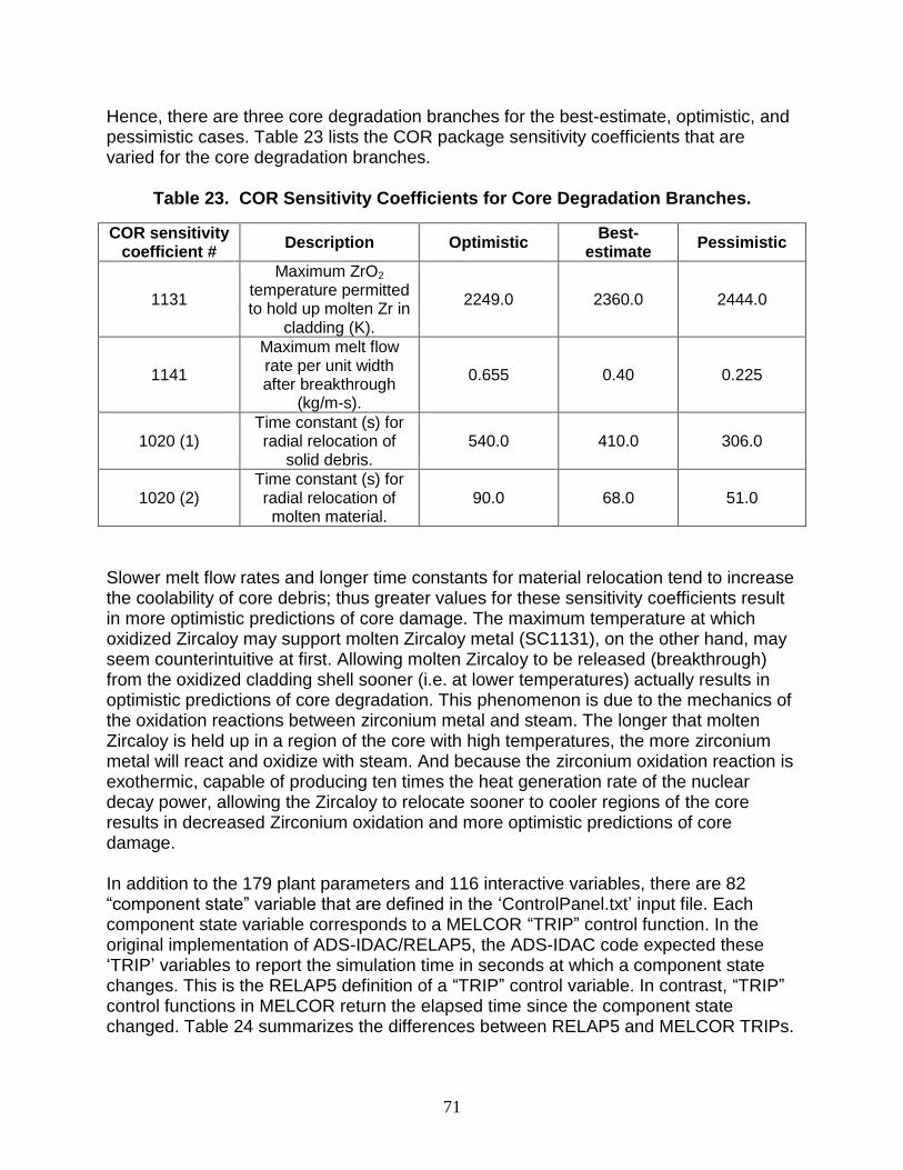
71

Hence, there are three core degradation branches for the best-estimate, optimistic, and pessimistic cases. Table 23 lists the COR package sensitivity coefficients that are varied for the core degradation branches.

Table 23. COR Sensitivity Coefficients for Core Degradation Branches.

COR sensitivity coefficient #

Description Optimistic Best-

estimate Pessimistic

1131

Maximum ZrO2

temperature permitted to hold up molten Zr in

cladding (K).

2249.0 2360.0 2444.0

1141

Maximum melt flow rate per unit width after breakthrough

(kg/m-s).

0.655 0.40 0.225

1020 (1) Time constant (s) for radial relocation of

solid debris. 540.0 410.0 306.0

1020 (2) Time constant (s) for radial relocation of molten material.

90.0 68.0 51.0

Slower melt flow rates and longer time constants for material relocation tend to increase the coolability of core debris; thus greater values for these sensitivity coefficients result in more optimistic predictions of core damage. The maximum temperature at which oxidized Zircaloy may support molten Zircaloy metal (SC1131), on the other hand, may seem counterintuitive at first. Allowing molten Zircaloy to be released (breakthrough) from the oxidized cladding shell sooner (i.e. at lower temperatures) actually results in optimistic predictions of core degradation. This phenomenon is due to the mechanics of the oxidation reactions between zirconium metal and steam. The longer that molten Zircaloy is held up in a region of the core with high temperatures, the more zirconium metal will react and oxidize with steam. And because the zirconium oxidation reaction is exothermic, capable of producing ten times the heat generation rate of the nuclear decay power, allowing the Zircaloy to relocate sooner to cooler regions of the core results in decreased Zirconium oxidation and more optimistic predictions of core damage. In addition to the 179 plant parameters and 116 interactive variables, there are 82 “component state” variable that are defined in the ‘ControlPanel.txt’ input file. Each component state variable corresponds to a MELCOR “TRIP” control function. In the original implementation of ADS-IDAC/RELAP5, the ADS-IDAC code expected these ‘TRIP’ variables to report the simulation time in seconds at which a component state changes. This is the RELAP5 definition of a “TRIP” control variable. In contrast, “TRIP” control functions in MELCOR return the elapsed time since the component state changed. Table 24 summarizes the differences between RELAP5 and MELCOR TRIPs.

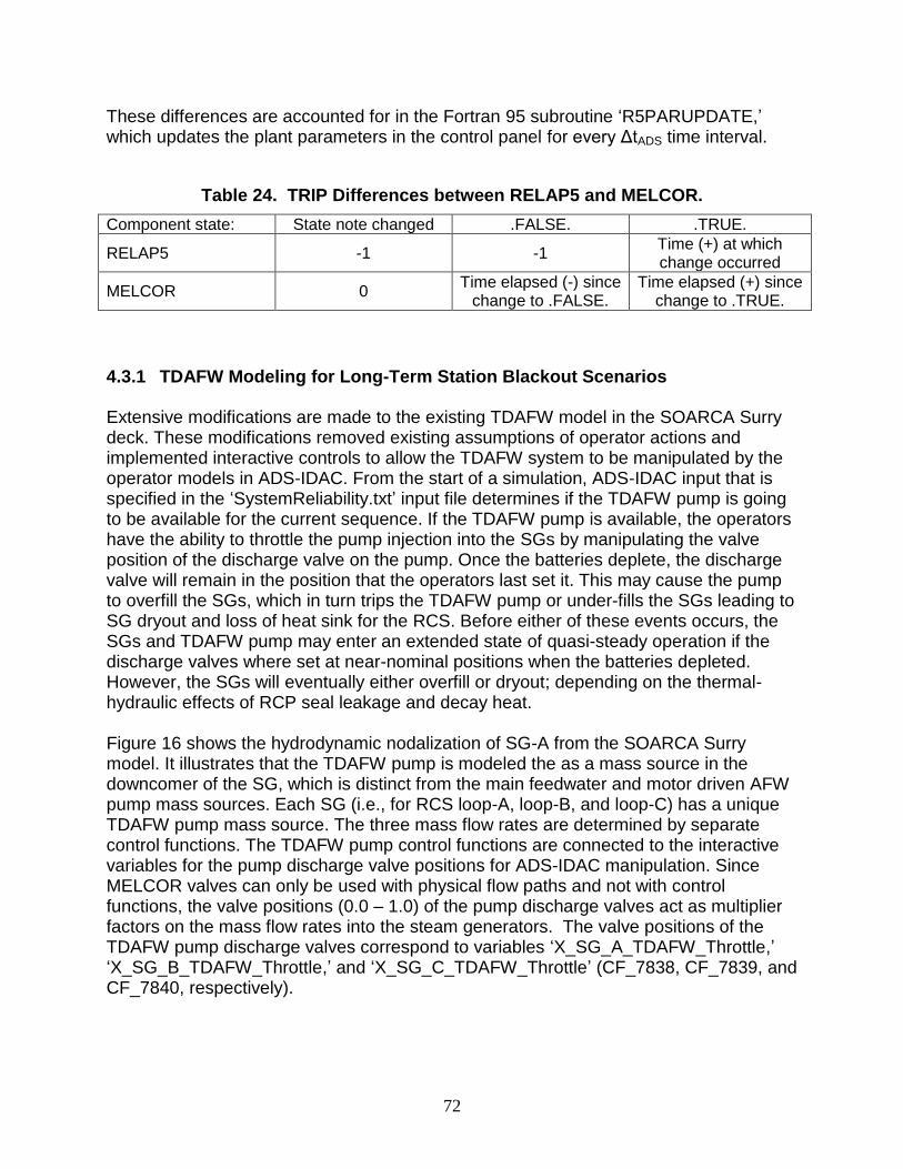
72

These differences are accounted for in the Fortran 95 subroutine ‘R5PARUPDATE,’ which updates the plant parameters in the control panel for every ΔtADS time interval.

Table 24. TRIP Differences between RELAP5 and MELCOR.

Component state: State note changed .FALSE. .TRUE.

RELAP5 -1 -1 Time (+) at which change occurred

MELCOR 0 Time elapsed (-) since

change to .FALSE. Time elapsed (+) since

change to .TRUE.

4.3.1 TDAFW Modeling for Long-Term Station Blackout Scenarios

Extensive modifications are made to the existing TDAFW model in the SOARCA Surry deck. These modifications removed existing assumptions of operator actions and implemented interactive controls to allow the TDAFW system to be manipulated by the operator models in ADS-IDAC. From the start of a simulation, ADS-IDAC input that is specified in the ‘SystemReliability.txt’ input file determines if the TDAFW pump is going to be available for the current sequence. If the TDAFW pump is available, the operators have the ability to throttle the pump injection into the SGs by manipulating the valve position of the discharge valve on the pump. Once the batteries deplete, the discharge valve will remain in the position that the operators last set it. This may cause the pump to overfill the SGs, which in turn trips the TDAFW pump or under-fills the SGs leading to SG dryout and loss of heat sink for the RCS. Before either of these events occurs, the SGs and TDAFW pump may enter an extended state of quasi-steady operation if the discharge valves where set at near-nominal positions when the batteries depleted. However, the SGs will eventually either overfill or dryout; depending on the thermal-hydraulic effects of RCP seal leakage and decay heat. Figure 16 shows the hydrodynamic nodalization of SG-A from the SOARCA Surry model. It illustrates that the TDAFW pump is modeled the as a mass source in the downcomer of the SG, which is distinct from the main feedwater and motor driven AFW pump mass sources. Each SG (i.e., for RCS loop-A, loop-B, and loop-C) has a unique TDAFW pump mass source. The three mass flow rates are determined by separate control functions. The TDAFW pump control functions are connected to the interactive variables for the pump discharge valve positions for ADS-IDAC manipulation. Since MELCOR valves can only be used with physical flow paths and not with control functions, the valve positions (0.0 – 1.0) of the pump discharge valves act as multiplier factors on the mass flow rates into the steam generators. The valve positions of the TDAFW pump discharge valves correspond to variables ‘X_SG_A_TDAFW_Throttle,’ ‘X_SG_B_TDAFW_Throttle,’ and ‘X_SG_C_TDAFW_Throttle’ (CF_7838, CF_7839, and CF_7840, respectively).

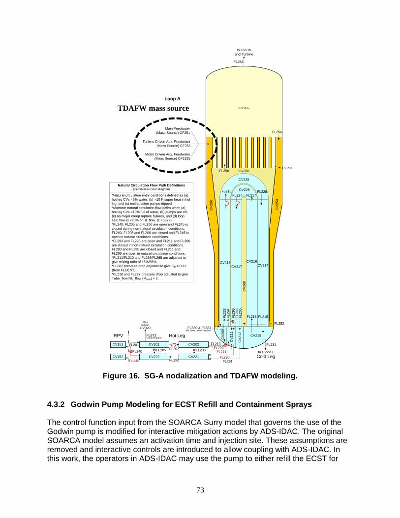
73

Figure 16. SG-A nodalization and TDAFW modeling.

4.3.2 Godwin Pump Modeling for ECST Refill and Containment Sprays The control function input from the SOARCA Surry model that governs the use of the Godwin pump is modified for interactive mitigation actions by ADS-IDAC. The original SOARCA model assumes an activation time and injection site. These assumptions are removed and interactive controls are introduced to allow coupling with ADS-IDAC. In this work, the operators in ADS-IDAC may use the pump to either refill the ECST for

RPV

CV

20

9

CV

21

1

CV

21

2

CV215

CV213CV217

CV216CV214

CV225

CV226

FL

23

3F

L2

94

FL218 FL228

FL215FL216

FL217FL227

FL

29

5

FL

26

5

CV202CV201

CV222 CV221

CV153

CV152

FL291

FL296

FL231

FL292

FL202FL240

FL201 FL210

FL211

FL250 CV260

CV265

CV

26

0

CV

25

0

CV

25

0

FL830 & FL831

FL252

FL253

FL254

FL283

SG Tube Creep Rupture

FL205

FL873Creep Rupture

SG A

Cubicle

CV020

FL206FL293

FL

26

6

FL245

Main Feedwater

(Mass Source) CF251

Turbine Driven Aux. Feedwater

(Mass Source) CF253

Motor Driven Aux. Feedwater

(Mass Source) CF1325

to CV270

and Turbine

to CV220

Hot Leg

Cold Leg

Loop A

Natural Circulation Flow Path Definitions(identified in red on diagram)

*Natural circulation entry conditions defined as (a)

hot leg CVs <5% water, (b) >10 K super heat in hot

leg, and (c) recirculation pumps tripped.

*Maintain natural circulation flow paths when (a)

hot leg CVs <10% full of water, (b) pumps are off,

(c) no major creep rupture failures, and (d) loop

seal flow is <20% of HL flow. (CF5672)

*FL240, FL205 and FL206 are open and FL245 is

closed during non-natural circulation conditions.

FL240, FL205 and FL206 are closed and FL245 is

open in natural circulation conditions.

*FL293 and FL295 are open and FL211 and FL266

are closed in non-natural circulation conditions.

FL293 and FL295 are closed and FL211 and

FL266 are open in natural circulation conditions.

*FL211/FL210 and FL266/FL265 are adjusted to

give mixing ratio of 15%/85%.

*FL202 pressure drop adjusted to give CD = 0.12

(from FLUENT).

*FL218 and FL227 pressure drop adjusted to give

Tube_flow/HL_flow (Mratio) = 2.

TDAFW mass source

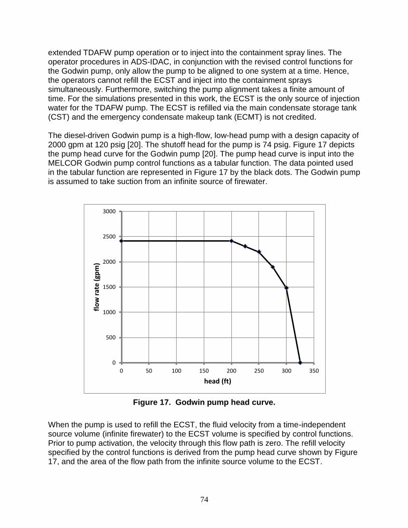
74

extended TDAFW pump operation or to inject into the containment spray lines. The operator procedures in ADS-IDAC, in conjunction with the revised control functions for the Godwin pump, only allow the pump to be aligned to one system at a time. Hence, the operators cannot refill the ECST and inject into the containment sprays simultaneously. Furthermore, switching the pump alignment takes a finite amount of time. For the simulations presented in this work, the ECST is the only source of injection water for the TDAFW pump. The ECST is refilled via the main condensate storage tank (CST) and the emergency condensate makeup tank (ECMT) is not credited. The diesel-driven Godwin pump is a high-flow, low-head pump with a design capacity of 2000 gpm at 120 psig [20]. The shutoff head for the pump is 74 psig. Figure 17 depicts the pump head curve for the Godwin pump [20]. The pump head curve is input into the MELCOR Godwin pump control functions as a tabular function. The data pointed used in the tabular function are represented in Figure 17 by the black dots. The Godwin pump is assumed to take suction from an infinite source of firewater.

Figure 17. Godwin pump head curve.

When the pump is used to refill the ECST, the fluid velocity from a time-independent source volume (infinite firewater) to the ECST volume is specified by control functions. Prior to pump activation, the velocity through this flow path is zero. The refill velocity specified by the control functions is derived from the pump head curve shown by Figure 17, and the area of the flow path from the infinite source volume to the ECST.

0

500

1000

1500

2000

2500

3000

0 50 100 150 200 250 300 350

flo

w r

ate

(gp

m)

head (ft)

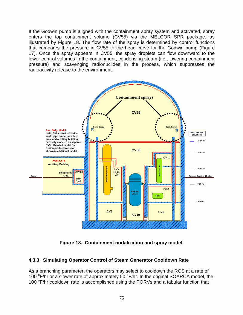
75

If the Godwin pump is aligned with the containment spray system and activated, spray enters the top containment volume (CV55) via the MELCOR SPR package, as illustrated by Figure 18. The flow rate of the spray is determined by control functions that compares the pressure in CV55 to the head curve for the Godwin pump (Figure 17). Once the spray appears in CV55, the spray droplets can flow downward to the lower control volumes in the containment, condensing steam (i.e., lowering containment pressure) and scavenging radionuclides in the process, which suppresses the radioactivity release to the environment.

Figure 18. Containment nodalization and spray model.

4.3.3 Simulating Operator Control of Steam Generator Cooldown Rate

As a branching parameter, the operators may select to cooldown the RCS at a rate of 100 oF/hr or a slower rate of approximately 50 oF/hr. In the original SOARCA model, the 100 oF/hr cooldown rate is accomplished using the PORVs and a tabular function that

CV41

CV's

20,30,

40

CV55

CV50

0.56 m

7.21 m

25.83 m

32.84 m

CV42

CV5CV5CV10

Pre

ss

uri

zer

Ste

am

Ge

nera

tor

PRT

16.85 m

Approx. Grade = 12.13 m

MELCOR Ref.

Elevations

Grade

CV800

LHSI

Safeguards

Area

Reactor

Vessel

Cont. Spray Cont. Spray

Aux. Bldg. Model

Note: Cable vault, electrical

vault, pipe tunnel, aux. feed.

area, and auxiliary building

currently modeled as separate

CV’s. Detailed model for

fission product transport

shown in additional model.

CV810-818

Auxiliary Building

Containment sprays

76

specifies pressure as a function of the time after cooldown was initiated. The tabular function specifies the thermodynamic conditions (control volume pressure) of a special control volume (CV282) that is used for the RCS cooldown process. This control volume is connected to the SGs via the PORV flow paths; hence, steam flows through the PORVs and into CV282. The cooldown process begins once the operators open the PORVs, and with the pressure of CV282 specified by the tabular function. The RCS then cools at a rate according to the pressure function.

Two separate pressure tables are necessary to simulate operator control of the cooldown rate. A control function determines which table is used to specify the cooldown rate. If ADS-IDAC specifies a PORV open fraction of 1.0 the 100 oF/hr cooldown table is used, and if ADS-IDAC specifies an open fraction of 0.5 then the 50 oF/hr table is used. The PORV position can also be changed to 0.0 to terminate the cooldown process. The cooldown will terminate once the pressure in the steam generators reaches 120 psig as well. The operators can terminate the depressurization before the 120 psig set-point, but the depressurization cannot continue past 120 psig since this value is hardcoded into the MELCOR model with tabular functions. Currently, table functions in the MELCOR database cannot be interactively modified in AIM. Table 25 shows data for the two pressure functions that, when used in unison with the PORV open fraction, determine the cooldown rate of the RCS once initiated by ADS-IDAC. If ADS-IDAC recloses the PORV, the cooldown will terminate and the SGs will re-pressurize

Table 25. Pressure vs. Time Functions for Different Cooldown Rates.

50 oF/hr cooldown rate (SG PORV VPI = 0.5)

100 oF/hr cooldown rate (SG PORV VPI = 1.0)

Time after operators open SG PORVs (s) Pressure (Pa) Pressure (Pa)

0.0 7.53x106 7.53x106

1800.0 6.23x106 4.93x106

3600.0 4.93x106 3.06x106

5400.0 3.06x106 1.81x106

7200.0 1.81x106 9.95x105

9000.0 9.95x105 9.32x105

10800.0 9.32x105 9.32x105

12400.0 9.32x105 9.32x105

1.0E+09 9.32x105 9.32x105

4.3.4 Estimating the Average Core Exit Thermocouple Temperature

The AIM demonstration model uses control functions to calculate an estimate of the average core exit thermocouple temperature, which corresponds to the CETCs variable in ‘ControlPanel.txt.’ This variable is used to determine the procedural transition from ECA-0.0 (EOPs) to the SAMGs. The operators transition to the SAMGs once MELCOR calculates a CETC temperature of 1200 oF.

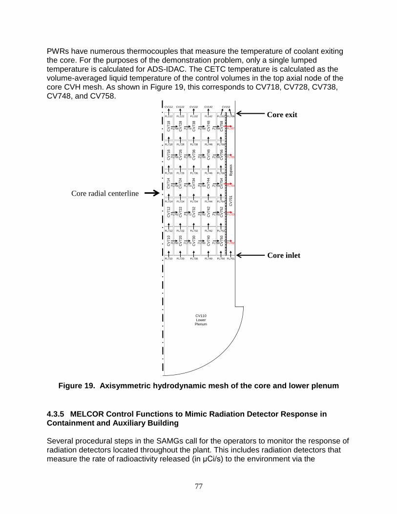
77

PWRs have numerous thermocouples that measure the temperature of coolant exiting the core. For the purposes of the demonstration problem, only a single lumped temperature is calculated for ADS-IDAC. The CETC temperature is calculated as the volume-averaged liquid temperature of the control volumes in the top axial node of the core CVH mesh. As shown in Figure 19, this corresponds to CV718, CV728, CV738, CV748, and CV758.

Figure 19. Axisymmetric hydrodynamic mesh of the core and lower plenum

4.3.5 MELCOR Control Functions to Mimic Radiation Detector Response in Containment and Auxiliary Building Several procedural steps in the SAMGs call for the operators to monitor the response of radiation detectors located throughout the plant. This includes radiation detectors that measure the rate of radioactivity released (in μCi/s) to the environment via the

CV110

Lower

Plenum

CV

71

0

CV

72

0

CV

73

0

CV

74

0

CV

75

0

CV

70

1

CV

71

2

CV

72

2

CV

73

2

CV

74

2

CV

75

2

CV

71

4

CV

72

4

CV

73

4

CV

74

4

CV

75

4

CV

71

6

CV

72

6

CV

73

6

CV

74

6

CV

75

6

CV

71

8

CV

72

8

CV

73

8

CV

74

8

CV

75

8

FL710 FL720 FL730 FL740 FL750

FL760 FL770 FL780 FL790

FL712 FL722 FL732 FL742 FL752

FL762 FL772 FL782 FL792

FL764 FL774 FL784 FL794

FL766 FL776 FL786 FL796

FL768 FL778 FL788 FL798

FL714 FL724 FL734 FL744 FL754

FL716 FL726 FL736 FL746 FL756

FL718 FL728 FL738 FL748 FL758

FL112 FL122 FL132 FL142 FL152 FL706

CV112 CV122 CV132 CV142 CV152

FL701

Byp

ass

FL707

Westinghouse 3-Loop PWR

CVH/FL Nodalization

FL705

FL704

FL703

FL702

0.0 m

0.93924 m

1.76396 m

2.0503 m

2.3800 m2.4181 m

3.01985 m

3.0643 m

3.4301 m

3.7958 m

4.1615 m

4.5273 m

4.8930 m

5.2588 m

5.6245 m

5.9902 m

6.3560 m

6.7217 m

108 208 308 408 508

109 209 309 409 509

110 210 310 410 510

111 211 311 411 511

112 212 312 412 512

113 213 313 413 513

114 214 314 414 514

115 215 315 415 515

116 216 316 416 516

117 217 317 417 517

106 206 306 406 506

104 204 304 404 504

103 203 303 403 503

102 202 302 402 502 602

101 201 301 401 501

Instrument

Thimble Tubes

(MELCOR NS),

HLST =

1.76396 m

Lower Core Plate

(MELCOR SS -

PLATE)

Lower Support

Columns

(MELCOR SS -

COLUMN)

Flow Mixer Plate

(MELCOR SS -

PLATEG)

Upper Support

Columns

(MELCOR SS -

COLUMN)

Bottom Nozzles &

Lower Core Plate

(MELCOR NS &

MELCOR SS -

PLATEG)

Active Fuel and

Control Rods

(Top Nozzles in

Axial Level 17,

Core Shroud and

Former in Ring 5)

Westinghouse 3-Loop PWR

Core Nodalization

DZLH =

0.13 m

R1 =

0.27134 m

R2 =

0.60715 m

R3 =

0.94846 m

R4 =

1.33587 m

R5 =

1.7005 m

R6 =

1.994 m

Core Cells

Lower Head

Nodalization

Flow Path Opens

at Shroud Failure

Flow Path

Controlled by

COR Blockage

Model

Legend

Core radial centerline

Core exit

Core inlet

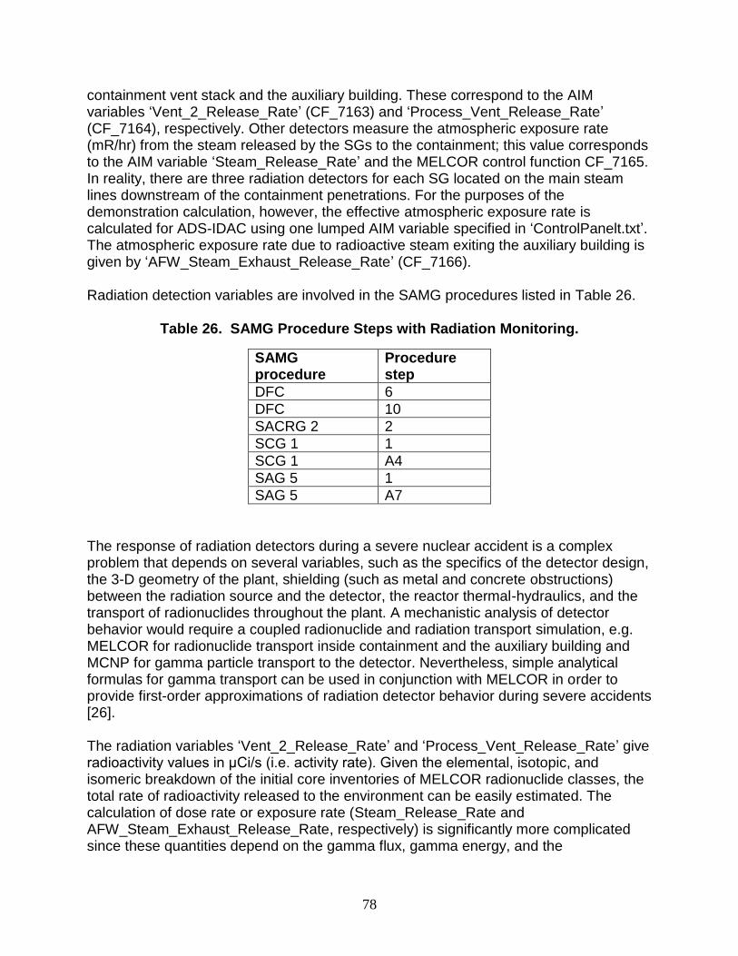
78

containment vent stack and the auxiliary building. These correspond to the AIM variables ‘Vent_2_Release_Rate’ (CF_7163) and ‘Process_Vent_Release_Rate’ (CF_7164), respectively. Other detectors measure the atmospheric exposure rate (mR/hr) from the steam released by the SGs to the containment; this value corresponds to the AIM variable ‘Steam_Release_Rate’ and the MELCOR control function CF_7165. In reality, there are three radiation detectors for each SG located on the main steam lines downstream of the containment penetrations. For the purposes of the demonstration calculation, however, the effective atmospheric exposure rate is calculated for ADS-IDAC using one lumped AIM variable specified in ‘ControlPanelt.txt’. The atmospheric exposure rate due to radioactive steam exiting the auxiliary building is given by ‘AFW_Steam_Exhaust_Release_Rate’ (CF_7166). Radiation detection variables are involved in the SAMG procedures listed in Table 26.

Table 26. SAMG Procedure Steps with Radiation Monitoring.

SAMG procedure

Procedure step

DFC 6

DFC 10

SACRG 2 2

SCG 1 1

SCG 1 A4

SAG 5 1

SAG 5 A7

The response of radiation detectors during a severe nuclear accident is a complex problem that depends on several variables, such as the specifics of the detector design, the 3-D geometry of the plant, shielding (such as metal and concrete obstructions) between the radiation source and the detector, the reactor thermal-hydraulics, and the transport of radionuclides throughout the plant. A mechanistic analysis of detector behavior would require a coupled radionuclide and radiation transport simulation, e.g. MELCOR for radionuclide transport inside containment and the auxiliary building and MCNP for gamma particle transport to the detector. Nevertheless, simple analytical formulas for gamma transport can be used in conjunction with MELCOR in order to provide first-order approximations of radiation detector behavior during severe accidents [26]. The radiation variables ‘Vent_2_Release_Rate’ and ‘Process_Vent_Release_Rate’ give radioactivity values in μCi/s (i.e. activity rate). Given the elemental, isotopic, and isomeric breakdown of the initial core inventories of MELCOR radionuclide classes, the total rate of radioactivity released to the environment can be easily estimated. The calculation of dose rate or exposure rate (Steam_Release_Rate and AFW_Steam_Exhaust_Release_Rate, respectively) is significantly more complicated since these quantities depend on the gamma flux, gamma energy, and the

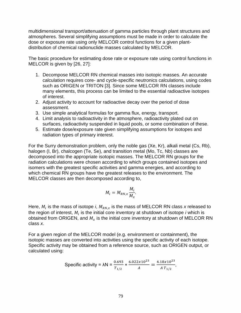
79

multidimensional transport/attenuation of gamma particles through plant structures and atmospheres. Several simplifying assumptions must be made in order to calculate the dose or exposure rate using only MELCOR control functions for a given plant-distribution of chemical radionuclide masses calculated by MELCOR. The basic procedure for estimating dose rate or exposure rate using control functions in MELCOR is given by [26, 27]:

1. Decompose MELCOR RN chemical masses into isotopic masses. An accurate calculation requires core- and cycle-specific neutronics calculations, using codes such as ORIGEN or TRITON [3]. Since some MELCOR RN classes include many elements, this process can be limited to the essential radioactive isotopes of interest.

2. Adjust activity to account for radioactive decay over the period of dose assessment.

3. Use simple analytical formulas for gamma flux, energy, transport. 4. Limit analysis to radioactivity in the atmosphere, radioactivity plated out on

surfaces, radioactivity suspended in liquid pools, or some combination of these. 5. Estimate dose/exposure rate given simplifying assumptions for isotopes and

radiation types of primary interest. For the Surry demonstration problem, only the noble gas (Xe, Kr), alkali metal (Cs, Rb), halogen (I, Br), chalcogen (Te, Se), and transition metal (Mo, Tc, Nb) classes are decomposed into the appropriate isotopic masses. The MELCOR RN groups for the radiation calculations were chosen according to which groups contained isotopes and isomers with the greatest specific activities and gamma energies, and according to which chemical RN groups have the greatest releases to the environment. The MELCOR classes are then decomposed according to,

Here, is the mass of isotope i, is the mass of MELCOR RN class x released to

the region of interest, is the initial core inventory at shutdown of isotope i which is

obtained from ORIGEN, and is the initial core inventory at shutdown of MELCOR RN class x. For a given region of the MELCOR model (e.g. environment or containment), the isotopic masses are converted into activities using the specific activity of each isotope. Specific activity may be obtained from a reference source, such as ORIGEN output, or calculated using:

Specific activity = λN =

,

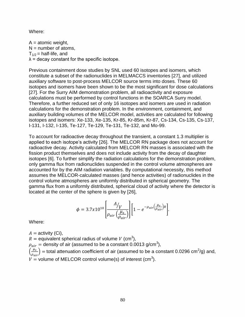
80

Where: A = atomic weight, N = number of atoms, T1/2 = half-life, and λ = decay constant for the specific isotope. Previous containment dose studies by SNL used 60 isotopes and isomers, which constitute a subset of the radionuclides in MELMACCS inventories [27], and utilized auxiliary software to post-process MELCOR source terms into doses. These 60 isotopes and isomers have been shown to be the most significant for dose calculations [27]. For the Surry AIM demonstration problem, all radioactivity and exposure calculations must be performed by control functions in the SOARCA Surry model. Therefore, a further reduced set of only 16 isotopes and isomers are used in radiation calculations for the demonstration problem. In the environment, containment, and auxiliary building volumes of the MELCOR model, activities are calculated for following isotopes and isomers: Xe-133, Xe-135, Kr-85, Kr-85m, Kr-87, Cs-134, Cs-135, Cs-137, I-131, I-132, I-135, Te-127, Te-129, Te-131, Te-132, and Mo-99. To account for radioactive decay throughout the transient, a constant 1.3 multiplier is applied to each isotope’s activity [26]. The MELCOR RN package does not account for radioactive decay. Activity calculated from MELCOR RN masses is associated with the fission product themselves and does not include activity from the decay of daughter isotopes [6]. To further simplify the radiation calculations for the demonstration problem, only gamma flux from radionuclides suspended in the control volume atmospheres are accounted for by the AIM radiation variables. By computational necessity, this method assumes the MELCOR-calculated masses (and hence activities) of radionuclides in the control volume atmospheres are uniformly distributed in spherical geometry. The gamma flux from a uniformly distributed, spherical cloud of activity where the detector is located at the center of the sphere is given by [26],

[ ⁄

(

)] [

(

) ]

Where:

activity (Ci), equivalent spherical radius of volume (cm3),

density of air (assumed to be a constant 0.0013 g/cm3),

(

) total attenuation coefficient of air (assumed to be a constant 0.0296 cm2/g) and,

volume of MELCOR control volume(s) of interest (cm3).

81

Once the gamma flux is estimated, the dose rate can be calculated according to,

(

)

In this expression, is the dose rate (rad/hr) and E is the gamma particle energy (MeV). For the calculation of exposure rate in the demonstration problem, the gamma flux is assumed to be mono-energetic. It is assumed that the energies of all gamma particles from gamma-emitting isotopes can be represented by a single lumped energy of 0.605 MeV. Finally, given the estimated dose rate in the region of interest, the exposure rate may be calculated: 1.141 R is equivalent to 1.0 rad in air.

82

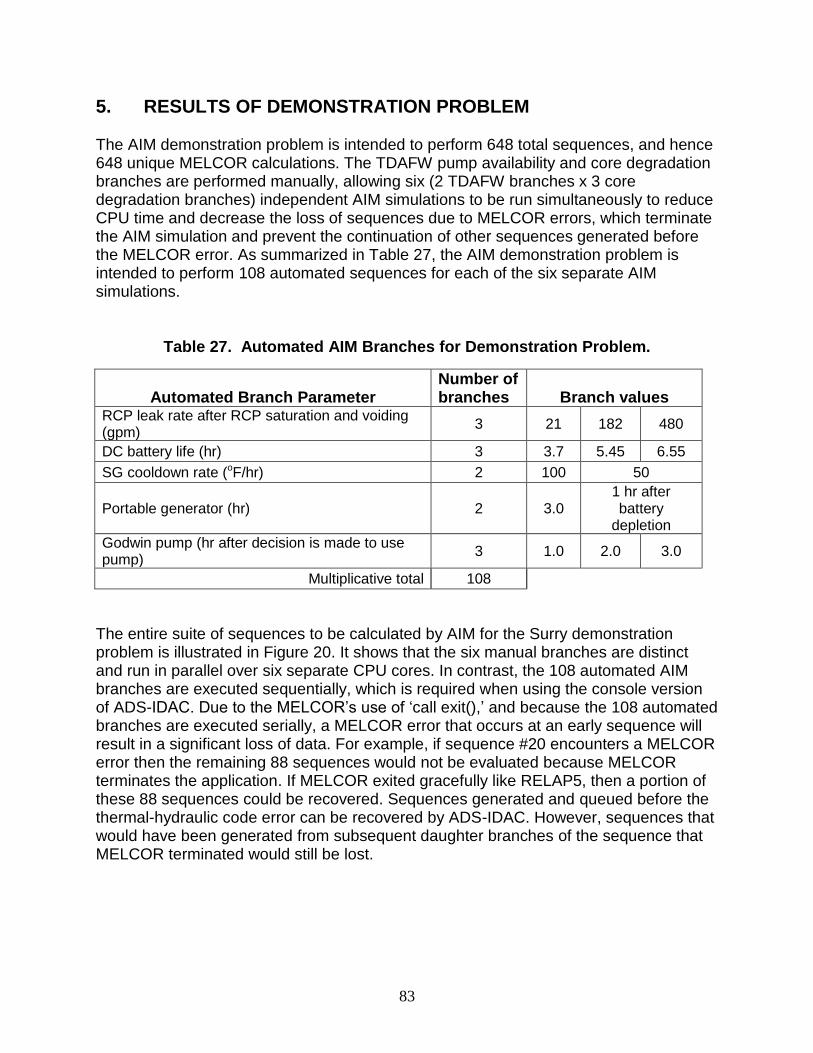
83

5. RESULTS OF DEMONSTRATION PROBLEM The AIM demonstration problem is intended to perform 648 total sequences, and hence 648 unique MELCOR calculations. The TDAFW pump availability and core degradation branches are performed manually, allowing six (2 TDAFW branches x 3 core degradation branches) independent AIM simulations to be run simultaneously to reduce CPU time and decrease the loss of sequences due to MELCOR errors, which terminate the AIM simulation and prevent the continuation of other sequences generated before the MELCOR error. As summarized in Table 27, the AIM demonstration problem is intended to perform 108 automated sequences for each of the six separate AIM simulations.

Table 27. Automated AIM Branches for Demonstration Problem.

Automated Branch Parameter Number of branches Branch values

RCP leak rate after RCP saturation and voiding (gpm)

3 21 182 480

DC battery life (hr) 3 3.7 5.45 6.55

SG cooldown rate (oF/hr) 2 100 50

Portable generator (hr) 2 3.0 1 hr after battery

depletion

Godwin pump (hr after decision is made to use pump)

3 1.0 2.0 3.0

Multiplicative total 108

The entire suite of sequences to be calculated by AIM for the Surry demonstration problem is illustrated in Figure 20. It shows that the six manual branches are distinct and run in parallel over six separate CPU cores. In contrast, the 108 automated AIM branches are executed sequentially, which is required when using the console version of ADS-IDAC. Due to the MELCOR’s use of ‘call exit(),’ and because the 108 automated branches are executed serially, a MELCOR error that occurs at an early sequence will result in a significant loss of data. For example, if sequence #20 encounters a MELCOR error then the remaining 88 sequences would not be evaluated because MELCOR terminates the application. If MELCOR exited gracefully like RELAP5, then a portion of these 88 sequences could be recovered. Sequences generated and queued before the thermal-hydraulic code error can be recovered by ADS-IDAC. However, sequences that would have been generated from subsequent daughter branches of the sequence that MELCOR terminated would still be lost.

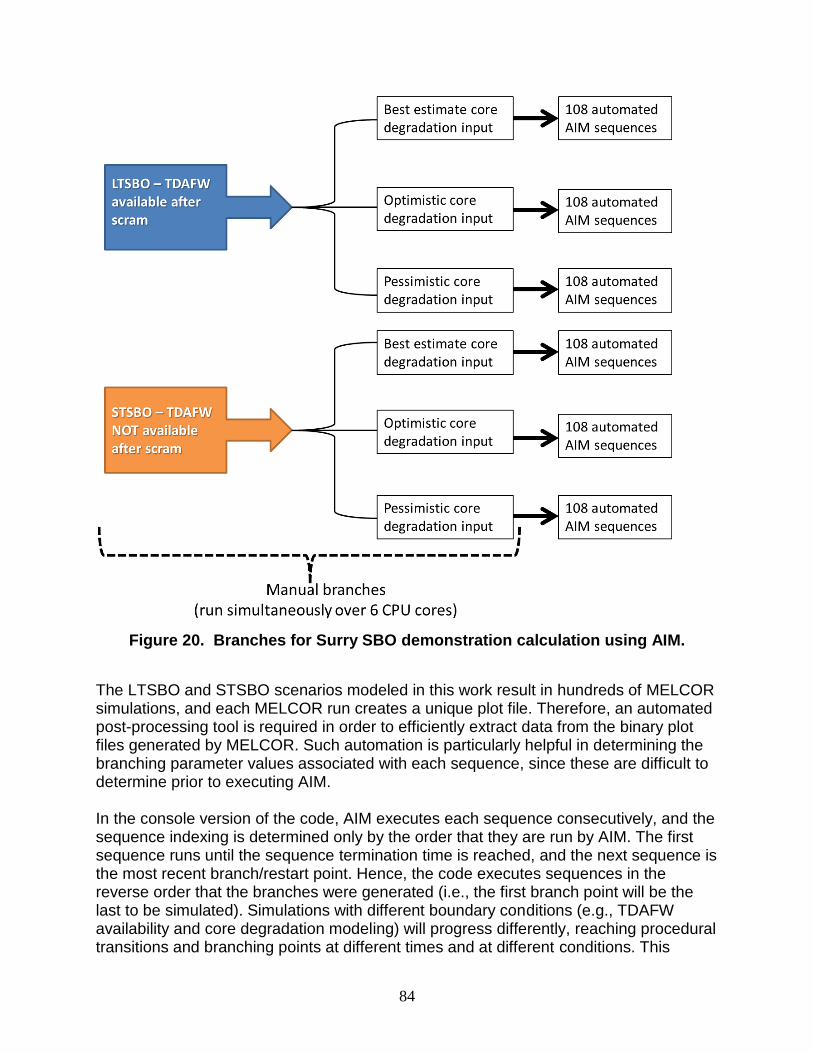
84

Figure 20. Branches for Surry SBO demonstration calculation using AIM.

The LTSBO and STSBO scenarios modeled in this work result in hundreds of MELCOR simulations, and each MELCOR run creates a unique plot file. Therefore, an automated post-processing tool is required in order to efficiently extract data from the binary plot files generated by MELCOR. Such automation is particularly helpful in determining the branching parameter values associated with each sequence, since these are difficult to determine prior to executing AIM. In the console version of the code, AIM executes each sequence consecutively, and the sequence indexing is determined only by the order that they are run by AIM. The first sequence runs until the sequence termination time is reached, and the next sequence is the most recent branch/restart point. Hence, the code executes sequences in the reverse order that the branches were generated (i.e., the first branch point will be the last to be simulated). Simulations with different boundary conditions (e.g., TDAFW availability and core degradation modeling) will progress differently, reaching procedural transitions and branching points at different times and at different conditions. This

85

causes the AIM tool to create restart points for additional sequences in a rather unpredictable fashion. Therefore, a single different branch point will preclude any preconceived concept of how each sequence number relates with the branching parameters. Further complicating the matter are the branching parameters that are not determined wholly by ADS-IDAC, but also by the thermal-hydraulic calculations in MELCOR. For example, the branch for the leakage rate from the RCP coolant pumps seals can only occur once MELCOR predicts that the pumps have voided and saturated. Another example is the time to activate the Godwin pump for ECST refill or core sprays. ADS-IDAC will only activate the Godwin pump once the operators enter the SAMGs, which is controlled by the MELCOR estimation of when the average core exit thermocouple temperature reaches 1200 oF. In order to post-process the binary data files, the APTPLOT program is used in batch mode, i.e. with the GUI suppressed, and the repetitive execution of APTPLOT for each plot variable is controlled by a Python script. Further, the Python script is run for each plot file by a master ‘.bash’ UNIX script. The end product from this process is a list of ASCII data files with each desired variable plotted versus the simulation time. The EDF capability in MELCOR can also generate text output directly, bypassing the need for a binary data post-processor, but this limits the available output to the EDF variables specified at execution. If the user did not select all the output data need for analysis, any additional data would need to be extracted from the binary plot files. A Perl script was also developed that reads the ASCII data files and creates summaries of important events and quantities for each sequence including: • Opening of the SG PORVS (timing and rate of the RCS cooldown), • RCP seal leakage flow rates, • TDAFW pump availability, • Godwin pump timing, • Godwin pump alignment and timing (ECST refill vs. containment sprays), • DC battery depletion, • Time at which the portable generator is connected, • Core exit temperatures, • Core damage progression–calculated as the mass fraction of the UO2 damaged, • Time of lower-head failure, • Time at which Zircaloy oxidation begins, • The total hydrogen mass generated from all in-vessel oxidation reactions, • The environmental release of cesium-iodide.

5.1. Partial Results from AIM Demonstration Problem Due to the MELCOR ‘call exit()’ issue and the ADS-IDAC problem with time-delayed branching of the Godwin pump activation time (Section 2.4.5), only a fraction of the initial 648 anticipated sequences were successfully simulated by AIM for the demonstration problem. The number of total successfully completed sequences is listed in Table 28.

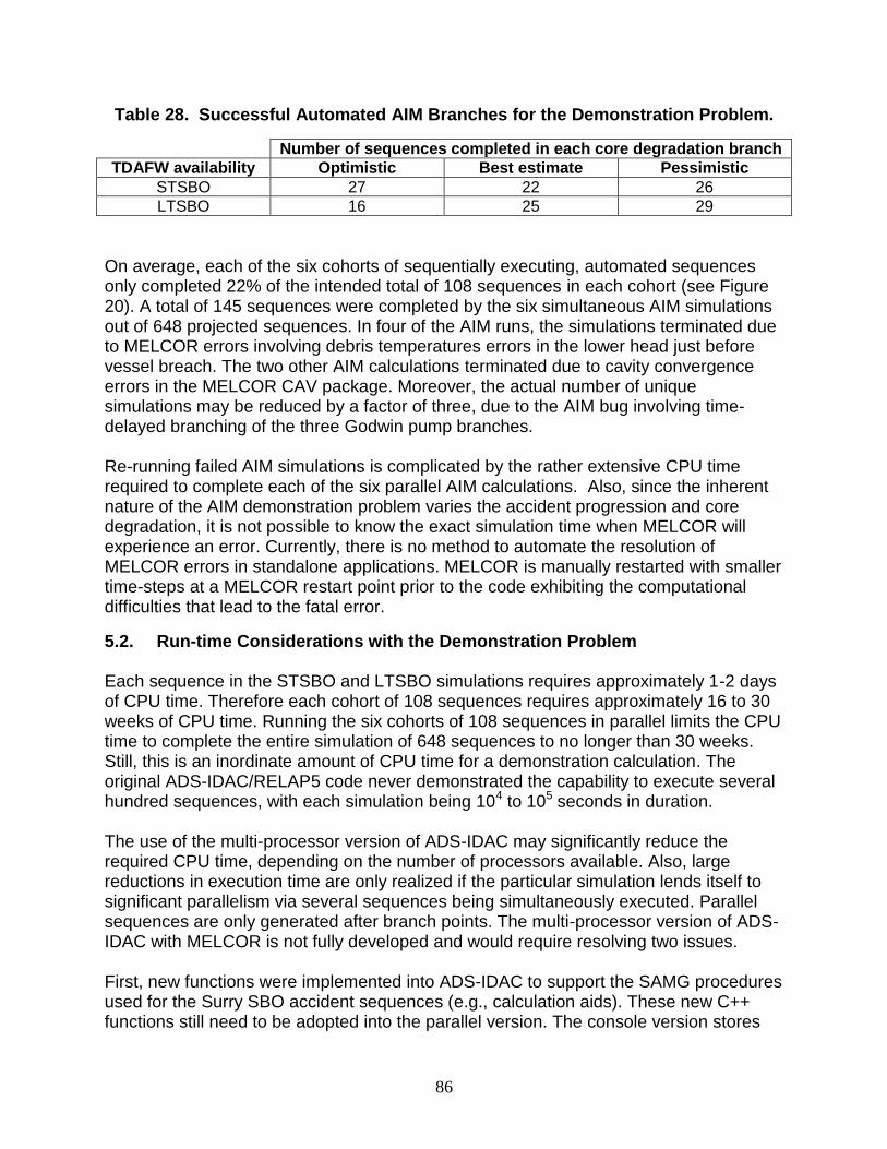
86

Table 28. Successful Automated AIM Branches for the Demonstration Problem.

Number of sequences completed in each core degradation branch

TDAFW availability Optimistic Best estimate Pessimistic

STSBO 27 22 26

LTSBO 16 25 29

On average, each of the six cohorts of sequentially executing, automated sequences only completed 22% of the intended total of 108 sequences in each cohort (see Figure 20). A total of 145 sequences were completed by the six simultaneous AIM simulations out of 648 projected sequences. In four of the AIM runs, the simulations terminated due to MELCOR errors involving debris temperatures errors in the lower head just before vessel breach. The two other AIM calculations terminated due to cavity convergence errors in the MELCOR CAV package. Moreover, the actual number of unique simulations may be reduced by a factor of three, due to the AIM bug involving time-delayed branching of the three Godwin pump branches. Re-running failed AIM simulations is complicated by the rather extensive CPU time required to complete each of the six parallel AIM calculations. Also, since the inherent nature of the AIM demonstration problem varies the accident progression and core degradation, it is not possible to know the exact simulation time when MELCOR will experience an error. Currently, there is no method to automate the resolution of MELCOR errors in standalone applications. MELCOR is manually restarted with smaller time-steps at a MELCOR restart point prior to the code exhibiting the computational difficulties that lead to the fatal error.

5.2. Run-time Considerations with the Demonstration Problem Each sequence in the STSBO and LTSBO simulations requires approximately 1-2 days of CPU time. Therefore each cohort of 108 sequences requires approximately 16 to 30 weeks of CPU time. Running the six cohorts of 108 sequences in parallel limits the CPU time to complete the entire simulation of 648 sequences to no longer than 30 weeks. Still, this is an inordinate amount of CPU time for a demonstration calculation. The original ADS-IDAC/RELAP5 code never demonstrated the capability to execute several hundred sequences, with each simulation being 104 to 105 seconds in duration. The use of the multi-processor version of ADS-IDAC may significantly reduce the required CPU time, depending on the number of processors available. Also, large reductions in execution time are only realized if the particular simulation lends itself to significant parallelism via several sequences being simultaneously executed. Parallel sequences are only generated after branch points. The multi-processor version of ADS-IDAC with MELCOR is not fully developed and would require resolving two issues. First, new functions were implemented into ADS-IDAC to support the SAMG procedures used for the Surry SBO accident sequences (e.g., calculation aids). These new C++ functions still need to be adopted into the parallel version. The console version stores

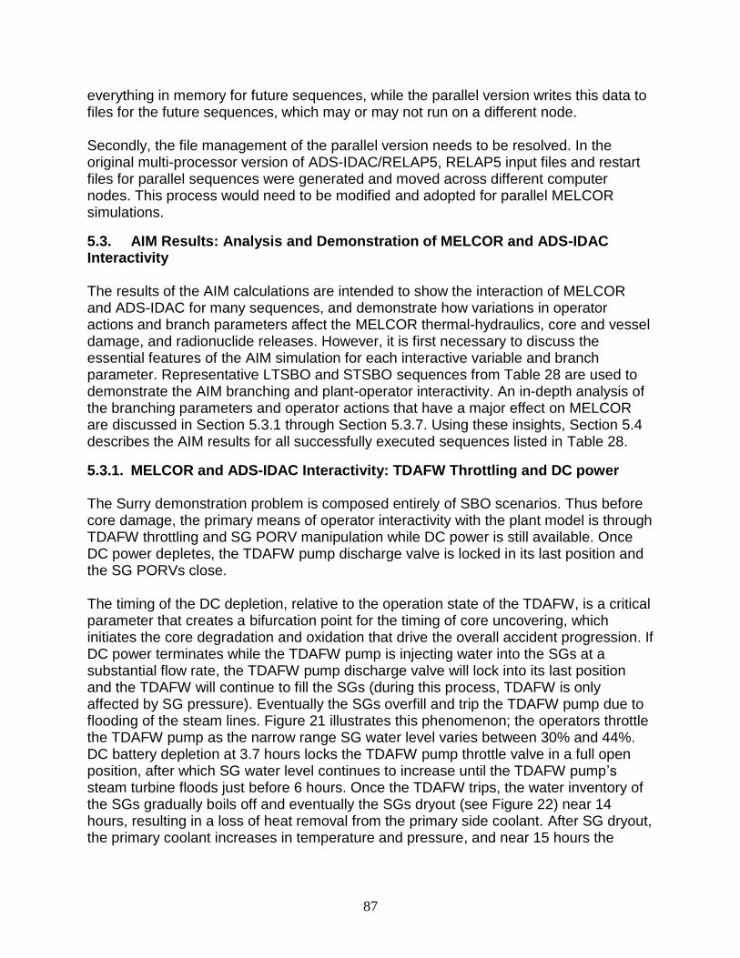
87

everything in memory for future sequences, while the parallel version writes this data to files for the future sequences, which may or may not run on a different node. Secondly, the file management of the parallel version needs to be resolved. In the original multi-processor version of ADS-IDAC/RELAP5, RELAP5 input files and restart files for parallel sequences were generated and moved across different computer nodes. This process would need to be modified and adopted for parallel MELCOR simulations.

5.3. AIM Results: Analysis and Demonstration of MELCOR and ADS-IDAC Interactivity The results of the AIM calculations are intended to show the interaction of MELCOR and ADS-IDAC for many sequences, and demonstrate how variations in operator actions and branch parameters affect the MELCOR thermal-hydraulics, core and vessel damage, and radionuclide releases. However, it is first necessary to discuss the essential features of the AIM simulation for each interactive variable and branch parameter. Representative LTSBO and STSBO sequences from Table 28 are used to demonstrate the AIM branching and plant-operator interactivity. An in-depth analysis of the branching parameters and operator actions that have a major effect on MELCOR are discussed in Section 5.3.1 through Section 5.3.7. Using these insights, Section 5.4 describes the AIM results for all successfully executed sequences listed in Table 28.

5.3.1. MELCOR and ADS-IDAC Interactivity: TDAFW Throttling and DC power The Surry demonstration problem is composed entirely of SBO scenarios. Thus before core damage, the primary means of operator interactivity with the plant model is through TDAFW throttling and SG PORV manipulation while DC power is still available. Once DC power depletes, the TDAFW pump discharge valve is locked in its last position and the SG PORVs close. The timing of the DC depletion, relative to the operation state of the TDAFW, is a critical parameter that creates a bifurcation point for the timing of core uncovering, which initiates the core degradation and oxidation that drive the overall accident progression. If DC power terminates while the TDAFW pump is injecting water into the SGs at a substantial flow rate, the TDAFW pump discharge valve will lock into its last position and the TDAFW will continue to fill the SGs (during this process, TDAFW is only affected by SG pressure). Eventually the SGs overfill and trip the TDAFW pump due to flooding of the steam lines. Figure 21 illustrates this phenomenon; the operators throttle the TDAFW pump as the narrow range SG water level varies between 30% and 44%. DC battery depletion at 3.7 hours locks the TDAFW pump throttle valve in a full open position, after which SG water level continues to increase until the TDAFW pump’s steam turbine floods just before 6 hours. Once the TDAFW trips, the water inventory of the SGs gradually boils off and eventually the SGs dryout (see Figure 22) near 14 hours, resulting in a loss of heat removal from the primary side coolant. After SG dryout, the primary coolant increases in temperature and pressure, and near 15 hours the

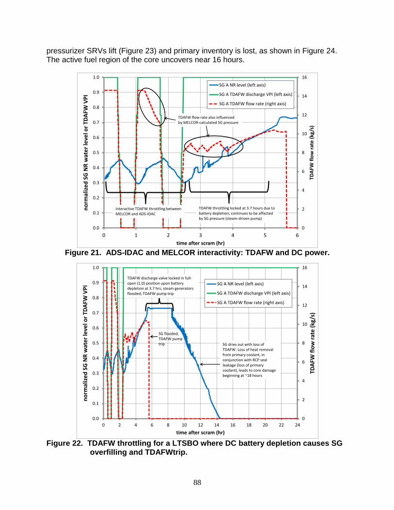
88

pressurizer SRVs lift (Figure 23) and primary inventory is lost, as shown in Figure 24. The active fuel region of the core uncovers near 16 hours.

Figure 21. ADS-IDAC and MELCOR interactivity: TDAFW and DC power.

Figure 22. TDAFW throttling for a LTSBO where DC battery depletion causes SG

overfilling and TDAFWtrip.

0

2

4

6

8

10

12

14

16

0.0

0.1

0.2

0.3

0.4

0.5

0.6

0.7

0.8

0.9

1.0

0 1 2 3 4 5 6

TDA

FW f

low

rat

e (

kg/s

)

no

rmal

ize

d S

G N

R w

ate

r le

vel o

r TD

AFW

VP

I

time after scram (hr)

SG A NR level (left axis)

SG A TDAFW discharge VPI (left axis)

SG A TDAFW flow rate (right axis)

interactive TDAFW throttling between MELCOR and ADS-IDAC

TDAFW throttling locked at 3.7 hours due to battery depletion; continues to be affected by SG pressure (steam-driven pump)

TDAFW flow rate also influenced by MELCOR-calculated SG pressure

0

2

4

6

8

10

12

14

16

0.0

0.1

0.2

0.3

0.4

0.5

0.6

0.7

0.8

0.9

1.0

0 2 4 6 8 10 12 14 16 18 20 22 24

TDA

FW f

low

rat

e (

kg/s

)

no

rmal

ize

d S

G N

R w

ate

r le

vel o

r TD

AFW

VP

I





TDAFW discharge valve locked in full-open (1.0) position upon battery depletion at 3.7 hrs; steam generatorsflooded; TDAFW pump trip

SG flooded; TDAFW pump trip SG dries out with loss of

TDAFW. Loss of heat removal from primary coolant, in conjunction with RCP seal leakage (loss of primary coolant), leads to core damage beginning at ~18 hours

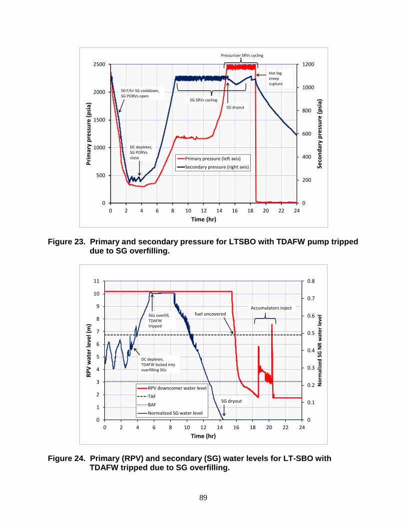
89

Figure 23. Primary and secondary pressure for LTSBO with TDAFW pump tripped

due to SG overfilling.

Figure 24. Primary (RPV) and secondary (SG) water levels for LT-SBO with

TDAFW tripped due to SG overfilling.

0

200

400

600

800

1000

1200

0

500

1000

1500

2000

2500

0 2 4 6 8 10 12 14 16 18 20 22 24

Seco

nd

ary

pre

ssu

re (

psi

a)

Pri

mar

y p

ress

ure

(p

sia)

Time (hr)

Primary pressure (left axis)

Secondary pressure (right axis)

Pressurizer SRVs cycling

SG SRVs cycling

50 F/hr SG cooldown, SG PORVs open

DC depletes, SG PORVs close

SG dryout

Hot leg creep rupture

0

0.1

0.2

0.3

0.4

0.5

0.6

0.7

0.8

0

1

2

3

4

5

6

7

8

9

10

11

0 2 4 6 8 10 12 14 16 18 20 22 24

No

rmal

ize

d S

G N

R w

ate

r le

vel

RP

V w

ate

r le

vel (

m)

Time (hr)

RPV downcomer water level

TAF

BAF

Normalized SG water level

SG dryout

fuel uncoveredAccumulators inject

DC depletes, TDAFW locked into overfilling SGs

SGs overfill, TDAFW tripped

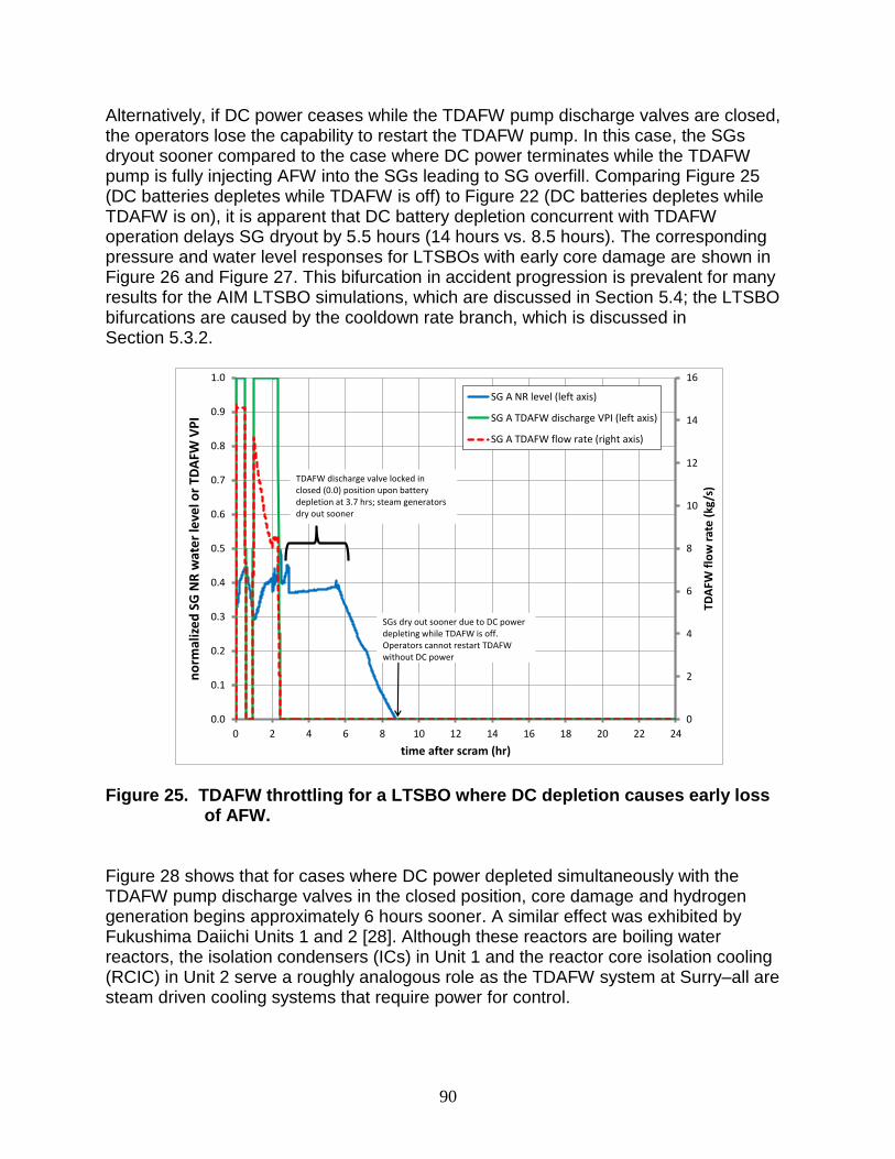
90

Alternatively, if DC power ceases while the TDAFW pump discharge valves are closed, the operators lose the capability to restart the TDAFW pump. In this case, the SGs dryout sooner compared to the case where DC power terminates while the TDAFW pump is fully injecting AFW into the SGs leading to SG overfill. Comparing Figure 25 (DC batteries depletes while TDAFW is off) to Figure 22 (DC batteries depletes while TDAFW is on), it is apparent that DC battery depletion concurrent with TDAFW operation delays SG dryout by 5.5 hours (14 hours vs. 8.5 hours). The corresponding pressure and water level responses for LTSBOs with early core damage are shown in Figure 26 and Figure 27. This bifurcation in accident progression is prevalent for many results for the AIM LTSBO simulations, which are discussed in Section 5.4; the LTSBO bifurcations are caused by the cooldown rate branch, which is discussed in Section 5.3.2.

Figure 25. TDAFW throttling for a LTSBO where DC depletion causes early loss

of AFW. Figure 28 shows that for cases where DC power depleted simultaneously with the TDAFW pump discharge valves in the closed position, core damage and hydrogen generation begins approximately 6 hours sooner. A similar effect was exhibited by Fukushima Daiichi Units 1 and 2 [28]. Although these reactors are boiling water reactors, the isolation condensers (ICs) in Unit 1 and the reactor core isolation cooling (RCIC) in Unit 2 serve a roughly analogous role as the TDAFW system at Surry–all are steam driven cooling systems that require power for control.

0

2

4

6

8

10

12

14

16

0.0

0.1

0.2

0.3

0.4

0.5

0.6

0.7

0.8

0.9

1.0

0 2 4 6 8 10 12 14 16 18 20 22 24

TDA

FW f

low

rat

e (

kg/s

)

no

rmal

ize

d S

G N

R w

ate

r le

vel o

r TD

AFW

VP

I





TDAFW discharge valve locked in closed (0.0) position upon battery depletion at 3.7 hrs; steam generators dry out sooner

SGs dry out sooner due to DC power depleting while TDAFW is off. Operators cannot restart TDAFW without DC power

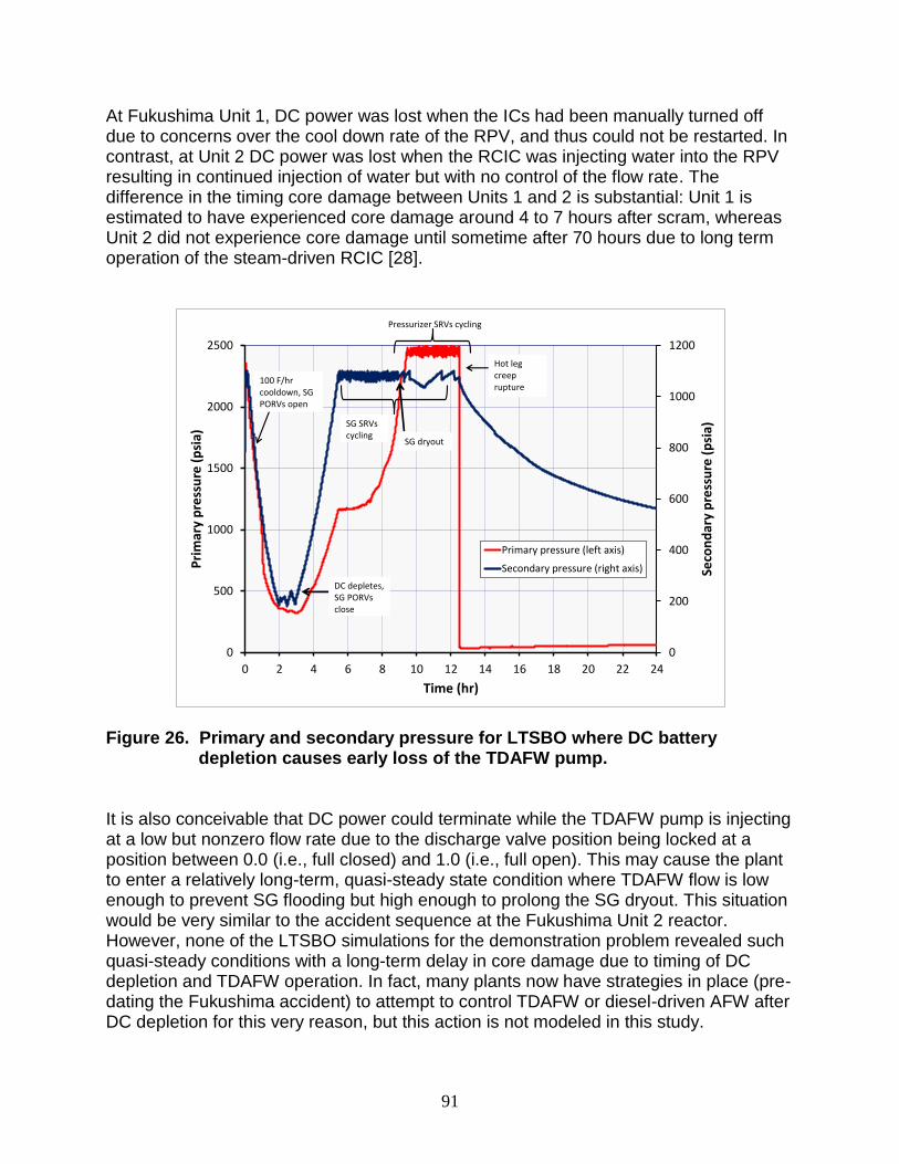
91

At Fukushima Unit 1, DC power was lost when the ICs had been manually turned off due to concerns over the cool down rate of the RPV, and thus could not be restarted. In contrast, at Unit 2 DC power was lost when the RCIC was injecting water into the RPV resulting in continued injection of water but with no control of the flow rate. The difference in the timing core damage between Units 1 and 2 is substantial: Unit 1 is estimated to have experienced core damage around 4 to 7 hours after scram, whereas Unit 2 did not experience core damage until sometime after 70 hours due to long term operation of the steam-driven RCIC [28].

Figure 26. Primary and secondary pressure for LTSBO where DC battery

depletion causes early loss of the TDAFW pump. It is also conceivable that DC power could terminate while the TDAFW pump is injecting at a low but nonzero flow rate due to the discharge valve position being locked at a position between 0.0 (i.e., full closed) and 1.0 (i.e., full open). This may cause the plant to enter a relatively long-term, quasi-steady state condition where TDAFW flow is low enough to prevent SG flooding but high enough to prolong the SG dryout. This situation would be very similar to the accident sequence at the Fukushima Unit 2 reactor. However, none of the LTSBO simulations for the demonstration problem revealed such quasi-steady conditions with a long-term delay in core damage due to timing of DC depletion and TDAFW operation. In fact, many plants now have strategies in place (pre-dating the Fukushima accident) to attempt to control TDAFW or diesel-driven AFW after DC depletion for this very reason, but this action is not modeled in this study.

0

200

400

600

800

1000

1200

0

500

1000

1500

2000

2500

0 2 4 6 8 10 12 14 16 18 20 22 24

Seco

nd

ary

pre

ssu

re (

psi

a)

Pri

mar

y p

ress

ure

(p

sia)

Time (hr)

Primary pressure (left axis)

Secondary pressure (right axis)

Pressurizer SRVs cycling

SG SRVs cycling

100 F/hrcooldown, SG PORVs open

DC depletes, SG PORVs close

SG dryout


92

Figure 27. Primary (RPV) and secondary (SG) water levels for LTSBO where DC

battery depletion causes early loss of the TDAFW pump.

Figure 28. Comparison of core oxidation timing: effect of the TDAFW pump on

accident progression (DC power ceases at 3.7 hours).

0

0.1

0.2

0.3

0.4

0.5

0.6

0.7

0.8

0

1

2

3

4

5

6

7

8

9

10

11

0 2 4 6 8 10 12 14 16 18 20 22 24

No

rmal

ize

d S

G N

R w

ate

r le

vel

RP

V w

ate

r le

vel (

m)

Time (hr)

RPV downcomer water level

TAF

BAF

Normalized SG water level

SG dryout

fuel uncovered

Accumulators injectDC depletes, TDAFW locked off

0

50

100

150

200

250

300

350

400

450

500

0 2 4 6 8 10 12 14 16 18 20 22 24

Inte

gral

hyd

roge

n g

en

era

ted

(kg

)

Time (hr)

DC depletion with TDAFW off

DC depletion with TDAFW on

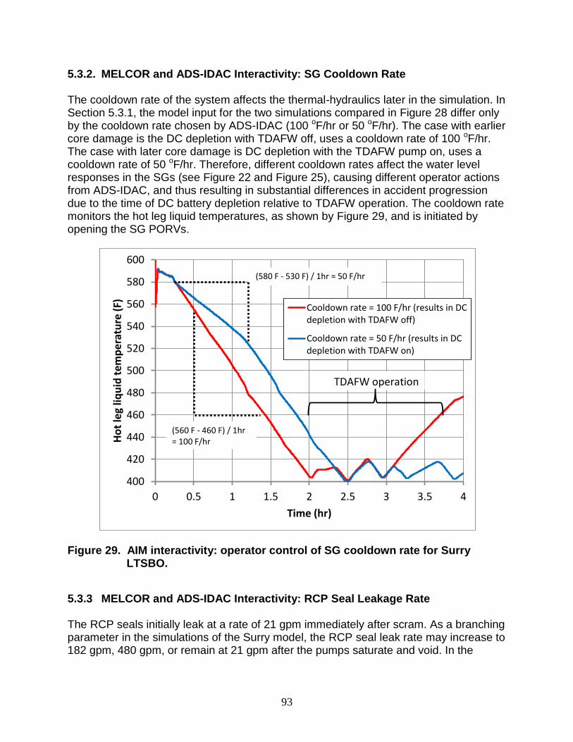
93

5.3.2. MELCOR and ADS-IDAC Interactivity: SG Cooldown Rate The cooldown rate of the system affects the thermal-hydraulics later in the simulation. In Section 5.3.1, the model input for the two simulations compared in Figure 28 differ only by the cooldown rate chosen by ADS-IDAC (100 oF/hr or 50 oF/hr). The case with earlier core damage is the DC depletion with TDAFW off, uses a cooldown rate of 100 oF/hr. The case with later core damage is DC depletion with the TDAFW pump on, uses a cooldown rate of 50 oF/hr. Therefore, different cooldown rates affect the water level responses in the SGs (see Figure 22 and Figure 25), causing different operator actions from ADS-IDAC, and thus resulting in substantial differences in accident progression due to the time of DC battery depletion relative to TDAFW operation. The cooldown rate monitors the hot leg liquid temperatures, as shown by Figure 29, and is initiated by opening the SG PORVs.

Figure 29. AIM interactivity: operator control of SG cooldown rate for Surry

LTSBO.

5.3.3 MELCOR and ADS-IDAC Interactivity: RCP Seal Leakage Rate The RCP seals initially leak at a rate of 21 gpm immediately after scram. As a branching parameter in the simulations of the Surry model, the RCP seal leak rate may increase to 182 gpm, 480 gpm, or remain at 21 gpm after the pumps saturate and void. In the

400

420

440

460

480

500

520

540

560

580

600

0 0.5 1 1.5 2 2.5 3 3.5 4

Ho

t le

g liq

uid

te

mp

era

ture

(F)

Time (hr)

Cooldown rate = 100 F/hr (results in DCdepletion with TDAFW off)

Cooldown rate = 50 F/hr (results in DCdepletion with TDAFW on)

(560 F - 460 F) / 1hr= 100 F/hr

TDAFW operation

(580 F - 530 F) / 1hr = 50 F/hr

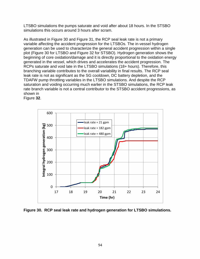
94

LTSBO simulations the pumps saturate and void after about 18 hours. In the STSBO simulations this occurs around 3 hours after scram. As illustrated in Figure 30 and Figure 31, the RCP seal leak rate is not a primary variable affecting the accident progression for the LTSBOs. The in-vessel hydrogen generation can be used to characterize the general accident progression within a single plot (Figure 30 for LTSBO and Figure 32 for STSBO). Hydrogen generation shows the beginning of core oxidation/damage and it is directly proportional to the oxidation energy generated in the vessel, which drives and accelerates the accident progression. The RCPs saturate and void late in the LTSBO simulations (18+ hours). Therefore, this branching variable contributes to the overall variability in final results. The RCP seal leak rate is not as significant as the SG cooldown, DC battery depletion, and the TDAFW pump throttling variables in the LTSBO simulations. And despite the RCP saturation and voiding occurring much earlier in the STSBO simulations, the RCP leak rate branch variable is not a central contributor to the STSBO accident progressions, as shown in Figure 32.

Figure 30. RCP seal leak rate and hydrogen generation for LTSBO simulations.

0

100

200

300

400

500

600

17 18 19 20 21 22 23 24

Inte

gral

hyd

roge

n g

en

era

tio

n (

kg)

Time (hr)

leak rate = 21 gpm

leak rate = 182 gpm

leak rate = 480 gpm

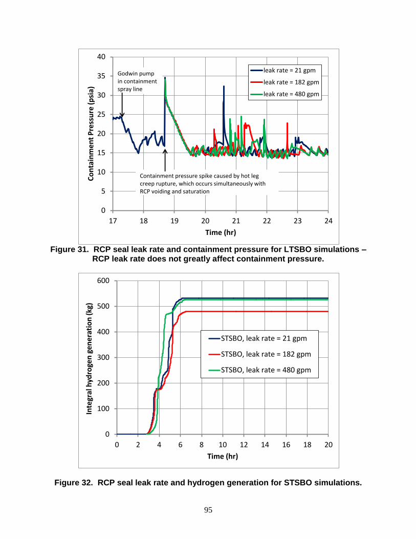
95

Figure 31. RCP seal leak rate and containment pressure for LTSBO simulations –

RCP leak rate does not greatly affect containment pressure.

Figure 32. RCP seal leak rate and hydrogen generation for STSBO simulations.

0

5

10

15

20

25

30

35

40

17 18 19 20 21 22 23 24

Co

nta

inm

en

t P

ress

ure

(p

sia)

Time (hr)

leak rate = 21 gpm

leak rate = 182 gpm

leak rate = 480 gpm

Containment pressure spike caused by hot leg creep rupture, which occurs simultaneously with RCP voiding and saturation

Godwin pump in containment spray line

0

100

200

300

400

500

600

0 2 4 6 8 10 12 14 16 18 20

Inte

gral

hyd

roge

n g

en

era

tio

n (

kg)

Time (hr)

STSBO, leak rate = 21 gpm



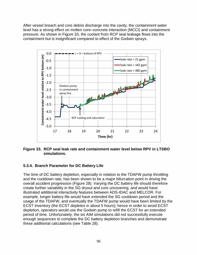
96

After vessel breach and core debris discharge into the cavity, the containment water level has a strong effect on molten core–concrete interaction (MCCI) and containment pressure. As shown in Figure 33, the coolant from RCP seal leakage flows into the containment but is insignificant compared to effect of the Godwin sprays.

Figure 33. RCP seal leak rate and containment water level below RPV in LTSBO simulations.

5.3.4. Branch Parameter for DC Battery Life The time of DC battery depletion, especially in relation to the TDAFW pump throttling and the cooldown rate, has been shown to be a major bifurcation point in driving the overall accident progression (Figure 28). Varying the DC battery life should therefore create further variability in the SG dryout and core uncovering, and would have illustrated additional interactivity features between ADS-IDAC and MELCOR. For example, longer battery life would have extended the SG cooldown period and the usage of the TDAFW, and eventually the TDAFW pump would have been limited by the ECST inventory (the ECST depletes in about 5 hours); hence in order to avoid ECST depletion, operators would use the Godwin pump to refill the ECST for an extended period of time. Unfortunately, the six AIM simulations did not successfully execute enough sequences to complete the DC battery depletion branches and demonstrate these additional calculations (see Table 28).

-5.0

-4.5

-4.0

-3.5

-3.0

-2.5

-2.0

-1.5

-1.0

-0.5

0.0

17 18 19 20 21 22 23 24

Co

nta

inm

ent

wat

er le

vel r

elat

ive

to R

PV

bo

tto

m (

m)

Time (hr)

leak rate = 21 gpm

leak rate = 182 gpm

leak rate = 480 gpm

RCP voiding and saturation

Godwin pump in containment spray line

z = 0 = bottom of RPV

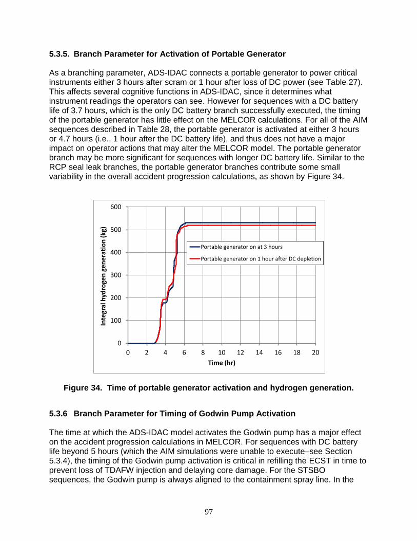
97

5.3.5. Branch Parameter for Activation of Portable Generator As a branching parameter, ADS-IDAC connects a portable generator to power critical instruments either 3 hours after scram or 1 hour after loss of DC power (see Table 27). This affects several cognitive functions in ADS-IDAC, since it determines what instrument readings the operators can see. However for sequences with a DC battery life of 3.7 hours, which is the only DC battery branch successfully executed, the timing of the portable generator has little effect on the MELCOR calculations. For all of the AIM sequences described in Table 28, the portable generator is activated at either 3 hours or 4.7 hours (i.e., 1 hour after the DC battery life), and thus does not have a major impact on operator actions that may alter the MELCOR model. The portable generator branch may be more significant for sequences with longer DC battery life. Similar to the RCP seal leak branches, the portable generator branches contribute some small variability in the overall accident progression calculations, as shown by Figure 34.

Figure 34. Time of portable generator activation and hydrogen generation.

5.3.6 Branch Parameter for Timing of Godwin Pump Activation The time at which the ADS-IDAC model activates the Godwin pump has a major effect on the accident progression calculations in MELCOR. For sequences with DC battery life beyond 5 hours (which the AIM simulations were unable to execute–see Section 5.3.4), the timing of the Godwin pump activation is critical in refilling the ECST in time to prevent loss of TDAFW injection and delaying core damage. For the STSBO sequences, the Godwin pump is always aligned to the containment spray line. In the

0

100

200

300

400

500

600

0 2 4 6 8 10 12 14 16 18 20

Inte

gral

hyd

roge

n g

en

era

tio

n (

kg)

Time (hr)

Portable generator on at 3 hours

Portable generator on 1 hour after DC depletion

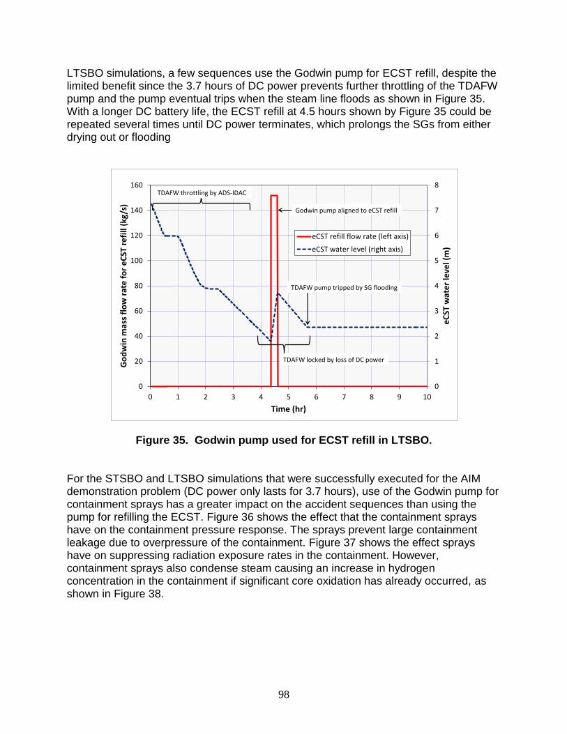
98

LTSBO simulations, a few sequences use the Godwin pump for ECST refill, despite the limited benefit since the 3.7 hours of DC power prevents further throttling of the TDAFW pump and the pump eventual trips when the steam line floods as shown in Figure 35. With a longer DC battery life, the ECST refill at 4.5 hours shown by Figure 35 could be repeated several times until DC power terminates, which prolongs the SGs from either drying out or flooding

Figure 35. Godwin pump used for ECST refill in LTSBO. For the STSBO and LTSBO simulations that were successfully executed for the AIM demonstration problem (DC power only lasts for 3.7 hours), use of the Godwin pump for containment sprays has a greater impact on the accident sequences than using the pump for refilling the ECST. Figure 36 shows the effect that the containment sprays have on the containment pressure response. The sprays prevent large containment leakage due to overpressure of the containment. Figure 37 shows the effect sprays have on suppressing radiation exposure rates in the containment. However, containment sprays also condense steam causing an increase in hydrogen concentration in the containment if significant core oxidation has already occurred, as shown in Figure 38.

0

1

2

3

4

5

6

7

8

0

20

40

60

80

100

120

140

160

0 1 2 3 4 5 6 7 8 9 10

eC

ST w

ate

r le

vel (

m)

Go

dw

in m

ass

flo

w r

ate

fo

r e

CST

ref

ill (

kg/s

)

Time (hr)

eCST refill flow rate (left axis)

eCST water level (right axis)

TDAFW throttling by ADS-IDAC

Godwin pump aligned to eCST refill

TDAFW locked by loss of DC power

TDAFW pump tripped by SG flooding

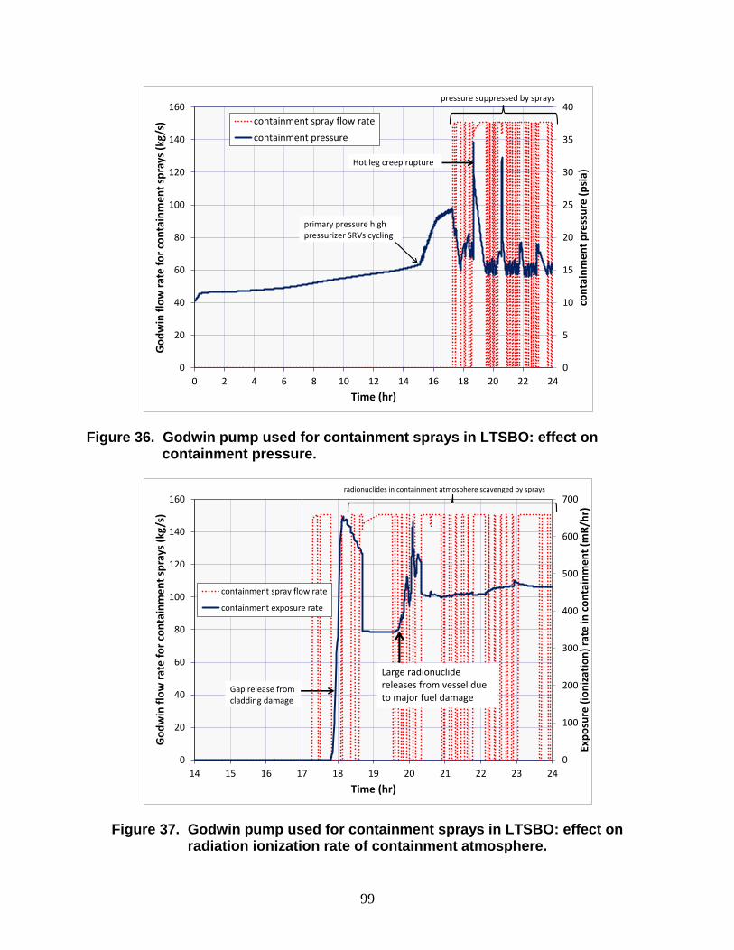
99

Figure 36. Godwin pump used for containment sprays in LTSBO: effect on

containment pressure.

Figure 37. Godwin pump used for containment sprays in LTSBO: effect on radiation ionization rate of containment atmosphere.

0

5

10

15

20

25

30

35

40

0

20

40

60

80

100

120

140

160

0 2 4 6 8 10 12 14 16 18 20 22 24

con

tain

me

nt

pre

ssu

re (

psi

a)

Go

dw

in f

low

rat

e f

or

con

tain

me

nt

spra

ys (

kg/s

)

Time (hr)

containment spray flow rate

containment pressure

pressure suppressed by sprays

primary pressure high pressurizer SRVs cycling


0

100

200

300

400

500

600

700

0

20

40

60

80

100

120

140

160

14 15 16 17 18 19 20 21 22 23 24

Exp

osu

re (

ion

izat

ion

) ra

te in

co

nta

inm

en

t (m

R/h

r)

Go

dw

in f

low

rat

e f

or

con

tain

me

nt

spra

ys (

kg/s

)

Time (hr)


containment exposure rate

radionuclides in containment atmosphere scavenged by sprays

Gap release from cladding damage

Large radionuclide releases from vessel due to major fuel damage

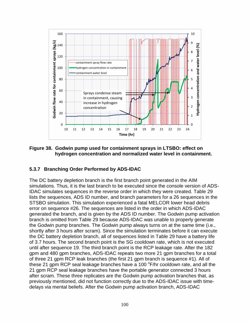
100

Figure 38. Godwin pump used for containment sprays in LTSBO: effect on

hydrogen concentration and normalized water level in containment.

5.3.7 Branching Order Performed by ADS-IDAC The DC battery depletion branch is the first branch point generated in the AIM simulations. Thus, it is the last branch to be executed since the console version of ADS-IDAC simulates sequences in the reverse order in which they were created. Table 29 lists the sequences, ADS ID number, and branch parameters for a 26 sequences in the STSBO simulation. This simulation experienced a fatal MELCOR lower head debris error on sequence #26. The sequences are listed in the order in which ADS-IDAC generated the branch, and is given by the ADS ID number. The Godwin pump activation branch is omitted from Table 29 because ADS-IDAC was unable to properly generate the Godwin pump branches. The Godwin pump always turns on at the same time (i.e., shortly after 3 hours after scram). Since the simulation terminates before it can execute the DC battery depletion branch, all of sequences listed in Table 29 have a battery life of 3.7 hours. The second branch point is the SG cooldown rate, which is not executed until after sequence 19. The third branch point is the RCP leakage rate. After the 182 gpm and 480 gpm branches, ADS-IDAC repeats two more 21 gpm branches for a total of three 21 gpm RCP leak branches (the first 21 gpm branch is sequence #1). All of these 21 gpm RCP seal leakage branches have a 100 oF/hr cooldown rate, and all the 21 gpm RCP seal leakage branches have the portable generator connected 3 hours after scram. These three replicates are the Godwin pump activation branches that, as previously mentioned, did not function correctly due to the ADS-IDAC issue with time-delays via mental beliefs. After the Godwin pump activation branch, ADS-IDAC

0

1

2

3

4

5

6

7

8

9

10

0

20

40

60

80

100

120

140

160

10 11 12 13 14 15 16 17 18 19 20 21 22 23 24

Hyd

roge

n c

on

cen

trat

ion

an

d w

ate

r le

vel (

%)

Go

dw

in f

low

rat

e f

or

con

tain

me

nt

spra

ys (

kg/s

)

Time (hr)


hydrogen concentration in containment

containment water level

Sprays condense steam in containment, causing increase in hydrogen concentration

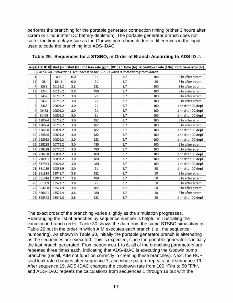
101

performs the branching for the portable generator connection timing (either 3 hours after scram or 1 hour after DC battery depletion). The portable generator branch does not suffer the time-delay issue as the Godwin pump branch due to differences in the input used to code the branching into ADS-IDAC.

Table 29. Sequences for a STSBO, in Order of Branch According to ADS ID #.

The exact order of the branching varies slightly as the simulation progresses. Rearranging the list of branches by sequence number is helpful in illustrating the variation in branch order. Table 30 shows the data from the same STSBO simulation as Table 29 but in the order in which AIM executes each branch (i.e., the sequence numbering). As shown in Table 30, initially the portable generator branch is alternating as the sequences are executed. This is expected, since the portable generator is initially the last branch generated. From sequences 1 to 6, all of the branching parameters are repeated three times each, indicating that ADS-IDAC is executing the Godwin pump branches (recall, AIM not function correctly in creating these branches). Next, the RCP seal leak rate changes after sequence 7, and whole pattern repeats until sequence 19. After sequence 19, ADS-IDAC changes the cooldown rate from 100 oF/hr to 50 oF/hr, and ADS-IDAC repeats the calculations from sequences 1 through 18 but with the

seq # ADS ID # tstart (s) tstart (hr) RCP leak rate (gpm) DC depl time (hr) SGcooldown rate (F/hr) Port. Generator (hr)

0 For ST-SBO simulations, sequence #0 is the LT-SBO which is immediately terminated

1 1 0.4 0.0 21 3.7 100 3 hr after scram

19 38 104.5 0.0 21 3.7 50 3 hr after scram

7 3235 10115.2 2.8 182 3.7 100 3 hr after scram

13 3235 10115.2 2.8 480 3.7 100 3 hr after scram

3 3452 10759.2 3.0 21 3.7 100 3 hr after scram

5 3452 10759.2 3.0 21 3.7 100 3 hr after scram

2 3468 10801.2 3.0 21 3.7 100 1 hr after DC depl

4 42473 10801.2 3.0 21 3.7 100 1 hr after DC depl

6 81478 10801.2 3.0 21 3.7 100 1 hr after DC depl

9 120684 10759.2 3.0 182 3.7 100 3 hr after scram

11 120684 10759.2 3.0 182 3.7 100 3 hr after scram

8 120700 10801.2 3.0 182 3.7 100 1 hr after DC depl

10 159806 10801.2 3.0 182 3.7 100 1 hr after DC depl

12 198912 10801.2 3.0 182 3.7 100 1 hr after DC depl

15 238228 10775.2 3.0 480 3.7 100 3 hr after scram

17 238228 10775.2 3.0 480 3.7 100 3 hr after scram

14 238238 10801.2 3.0 480 3.7 100 1 hr after DC depl

16 278091 10801.2 3.0 480 3.7 100 1 hr after DC depl

18 317944 10801.2 3.0 480 3.7 100 1 hr after DC depl

25 361119 10833.9 3.0 21 3.7 50 1 hr after DC depl

21 361814 13041.7 3.6 182 3.7 50 3 hr after scram

23 361814 13041.7 3.6 480 3.7 50 3 hr after scram

20 361989 13571.7 3.8 21 3.7 50 3 hr after scram

22 364298 13571.9 3.8 182 3.7 50 3 hr after scram

24 366621 13575.4 3.8 480 3.7 50 3 hr after scram

26 368503 13041.8 3.6 182 3.7 50 1 hr after DC depl

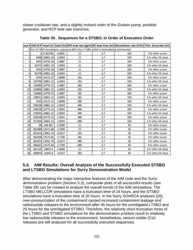
102

slower cooldown rate, and a slightly revised order of the Godwin pump, portable generator, and RCP leak rate branches.

Table 30. Sequences for a STSBO, in Order of Execution Order

5.4. AIM Results: Overall Analysis of the Successfully Executed STSBO and LTSBO Simulations for Surry Demonstration Model After demonstrating the major interactive features of the AIM code and the Surry demonstration problem (Section 5.3), composite plots of all successful results (see Table 28) can be created to analyze the overall trends of the AIM simulations. The LTSBO MELCOR simulations have a truncation time of 24 hours, and the STSBO simulations have a truncation time of 20 hours. In the Surry SOARCA analyses [20], over-pressurization of the containment caused increased containment leakage and radionuclide releases to the environment after 45 hours for the unmitigated LTSBO and 25 hours for the unmitigated STSBO. Therefore, the relatively short truncation times of the LTSBO and STSBO simulations for the demonstration problem result in relatively low radionuclide releases to the environment. Nonetheless, cesium-iodide (CsI) releases are still analyzed for all successfully executed sequences.

seq # ADS ID # tstart (s) tstart (hr) RCP leak rate (gpm) DC depl time (hr) SGcooldown rate (F/hr) Port. Generator (hr)

0 For ST-SBO simulations, sequence #0 is the LT-SBO which is immediately terminated

1 1 0.362781 0.0001 21 3.7 100 3 hr after scram

2 3468 10801.18 3.0003 21 3.7 100 1 hr after DC depl

3 3452 10759.18 2.9887 21 3.7 100 3 hr after scram

4 42473 10801.18 3.0003 21 3.7 100 1 hr after DC depl

5 3452 10759.18 2.9887 21 3.7 100 3 hr after scram

6 81478 10801.18 3.0003 21 3.7 100 1 hr after DC depl

7 3235 10115.15 2.8098 182 3.7 100 3 hr after scram

8 120700 10801.15 3.0003 182 3.7 100 1 hr after DC depl

9 120684 10759.15 2.9887 182 3.7 100 3 hr after scram

10 159806 10801.15 3.0003 182 3.7 100 1 hr after DC depl

11 120684 10759.15 2.9887 182 3.7 100 3 hr after scram

12 198912 10801.15 3.0003 182 3.7 100 1 hr after DC depl

13 3235 10115.15 2.8098 480 3.7 100 3 hr after scram

14 238238 10801.15 3.0003 480 3.7 100 1 hr after DC depl

15 238228 10775.15 2.9931 480 3.7 100 3 hr after scram

16 278091 10801.15 3.0003 480 3.7 100 1 hr after DC depl

17 238228 10775.15 2.9931 480 3.7 100 3 hr after scram

18 317944 10801.15 3.0003 480 3.7 100 1 hr after DC depl

19 38 104.492 0.0290 21 3.7 50 3 hr after scram

20 361989 13571.68 3.7699 21 3.7 50 3 hr after scram

21 361814 13041.74 3.6227 182 3.7 50 3 hr after scram

22 364298 13571.85 3.7700 182 3.7 50 3 hr after scram

23 361814 13041.74 3.6227 480 3.7 50 3 hr after scram

24 366621 13575.36 3.7709 480 3.7 50 3 hr after scram

25 361119 10833.9 3.0094 21 3.7 50 1 hr after DC depl

26 368503 13041.8 3.6227 182 3.7 50 1 hr after DC depl

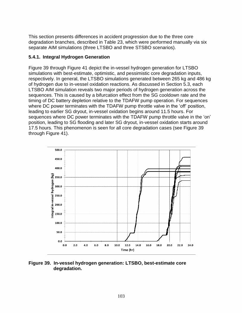
103

This section presents differences in accident progression due to the three core degradation branches, described in Table 23, which were performed manually via six separate AIM simulations (three LTSBO and three STSBO scenarios).

5.4.1. Integral Hydrogen Generation Figure 39 through Figure 41 depict the in-vessel hydrogen generation for LTSBO simulations with best-estimate, optimistic, and pessimistic core degradation inputs, respectively. In general, the LTSBO simulations generated between 265 kg and 486 kg of hydrogen due to in-vessel oxidation reactions. As discussed in Section 5.3, each LTSBO AIM simulation reveals two major periods of hydrogen generation across the sequences. This is caused by a bifurcation effect from the SG cooldown rate and the timing of DC battery depletion relative to the TDAFW pump operation. For sequences where DC power terminates with the TDAFW pump throttle valve in the ‘off’ position, leading to earlier SG dryout, in-vessel oxidation begins around 11.5 hours. For sequences where DC power terminates with the TDAFW pump throttle valve in the ‘on’ position, leading to SG flooding and later SG dryout, in-vessel oxidation starts around 17.5 hours. This phenomenon is seen for all core degradation cases (see Figure 39 through Figure 41).

Figure 39. In-vessel hydrogen generation: LTSBO, best-estimate core

degradation.

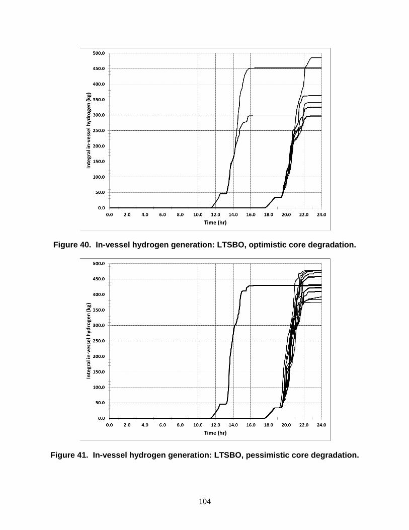
104

Figure 40. In-vessel hydrogen generation: LTSBO, optimistic core degradation.

Figure 41. In-vessel hydrogen generation: LTSBO, pessimistic core degradation.

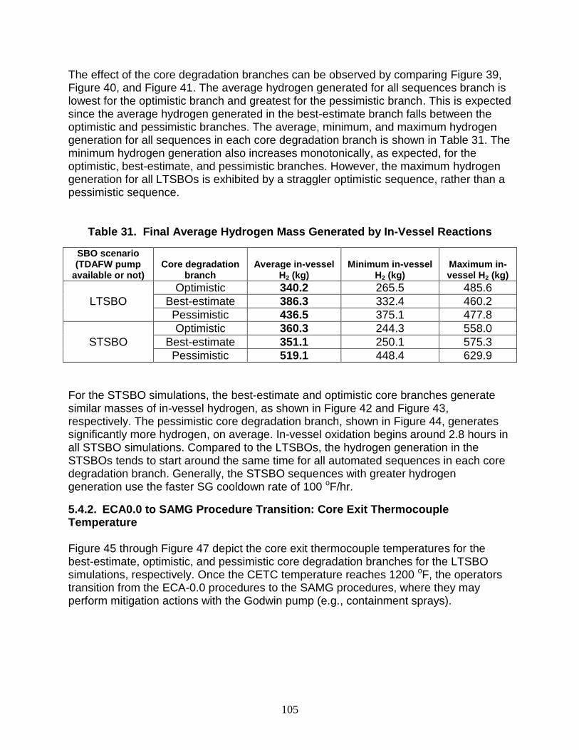
105

The effect of the core degradation branches can be observed by comparing Figure 39, Figure 40, and Figure 41. The average hydrogen generated for all sequences branch is lowest for the optimistic branch and greatest for the pessimistic branch. This is expected since the average hydrogen generated in the best-estimate branch falls between the optimistic and pessimistic branches. The average, minimum, and maximum hydrogen generation for all sequences in each core degradation branch is shown in Table 31. The minimum hydrogen generation also increases monotonically, as expected, for the optimistic, best-estimate, and pessimistic branches. However, the maximum hydrogen generation for all LTSBOs is exhibited by a straggler optimistic sequence, rather than a pessimistic sequence.

Table 31. Final Average Hydrogen Mass Generated by In-Vessel Reactions

SBO scenario (TDAFW pump

available or not) Core degradation

branch Average in-vessel

H2 (kg) Minimum in-vessel

H2 (kg) Maximum in-vessel H2 (kg)

LTSBO

Optimistic 340.2 265.5 485.6

Best-estimate 386.3 332.4 460.2

Pessimistic 436.5 375.1 477.8

STSBO

Optimistic 360.3 244.3 558.0

Best-estimate 351.1 250.1 575.3

Pessimistic 519.1 448.4 629.9

For the STSBO simulations, the best-estimate and optimistic core branches generate similar masses of in-vessel hydrogen, as shown in Figure 42 and Figure 43, respectively. The pessimistic core degradation branch, shown in Figure 44, generates significantly more hydrogen, on average. In-vessel oxidation begins around 2.8 hours in all STSBO simulations. Compared to the LTSBOs, the hydrogen generation in the STSBOs tends to start around the same time for all automated sequences in each core degradation branch. Generally, the STSBO sequences with greater hydrogen generation use the faster SG cooldown rate of 100 oF/hr.

5.4.2. ECA0.0 to SAMG Procedure Transition: Core Exit Thermocouple Temperature

Figure 45 through Figure 47 depict the core exit thermocouple temperatures for the best-estimate, optimistic, and pessimistic core degradation branches for the LTSBO simulations, respectively. Once the CETC temperature reaches 1200 oF, the operators transition from the ECA-0.0 procedures to the SAMG procedures, where they may perform mitigation actions with the Godwin pump (e.g., containment sprays).

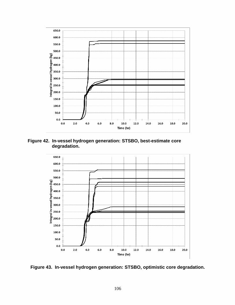
106

Figure 42. In-vessel hydrogen generation: STSBO, best-estimate core

degradation.

Figure 43. In-vessel hydrogen generation: STSBO, optimistic core degradation.

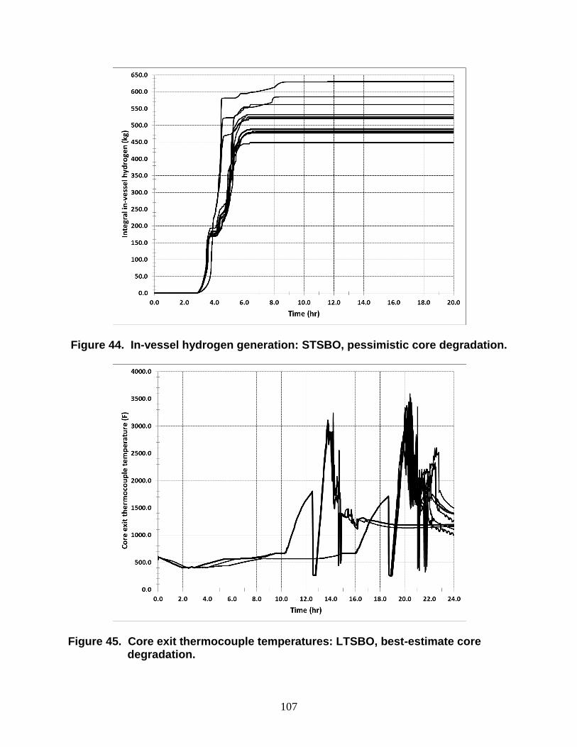
107

Figure 44. In-vessel hydrogen generation: STSBO, pessimistic core degradation.

Figure 45. Core exit thermocouple temperatures: LTSBO, best-estimate core

degradation.

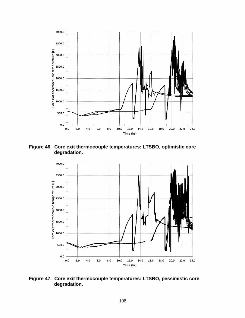
108

Figure 46. Core exit thermocouple temperatures: LTSBO, optimistic core degradation.

Figure 47. Core exit thermocouple temperatures: LTSBO, pessimistic core

degradation.

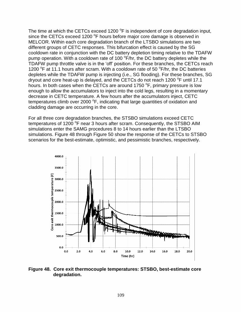
109

The time at which the CETCs exceed 1200 oF is independent of core degradation input, since the CETCs exceed 1200 oF hours before major core damage is observed in MELCOR. Within each core degradation branch of the LTSBO simulations are two different groups of CETC responses. This bifurcation effect is caused by the SG cooldown rate in conjunction with the DC battery depletion timing relative to the TDAFW pump operation. With a cooldown rate of 100 oF/hr, the DC battery depletes while the TDAFW pump throttle valve is in the ‘off’ position. For these branches, the CETCs reach 1200 oF at 11.1 hours after scram. With a cooldown rate of 50 oF/hr, the DC batteries depletes while the TDAFW pump is injecting (i.e., SG flooding). For these branches, SG dryout and core heat-up is delayed, and the CETCs do not reach 1200 oF until 17.1 hours. In both cases when the CETCs are around 1750 oF, primary pressure is low enough to allow the accumulators to inject into the cold legs, resulting in a momentary decrease in CETC temperature. A few hours after the accumulators inject, CETC temperatures climb over 2000 oF, indicating that large quantities of oxidation and cladding damage are occurring in the core. For all three core degradation branches, the STSBO simulations exceed CETC temperatures of 1200 oF near 3 hours after scram. Consequently, the STSBO AIM simulations enter the SAMG procedures 8 to 14 hours earlier than the LTSBO simulations. Figure 48 through Figure 50 show the response of the CETCs to STSBO scenarios for the best-estimate, optimistic, and pessimistic branches, respectively.

Figure 48. Core exit thermocouple temperatures: STSBO, best-estimate core

degradation.

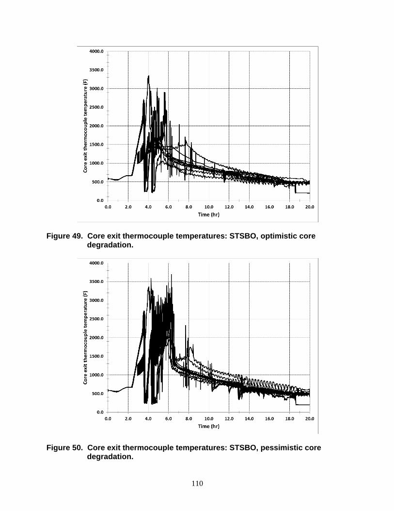
110

Figure 49. Core exit thermocouple temperatures: STSBO, optimistic core

degradation.

Figure 50. Core exit thermocouple temperatures: STSBO, pessimistic core

degradation.

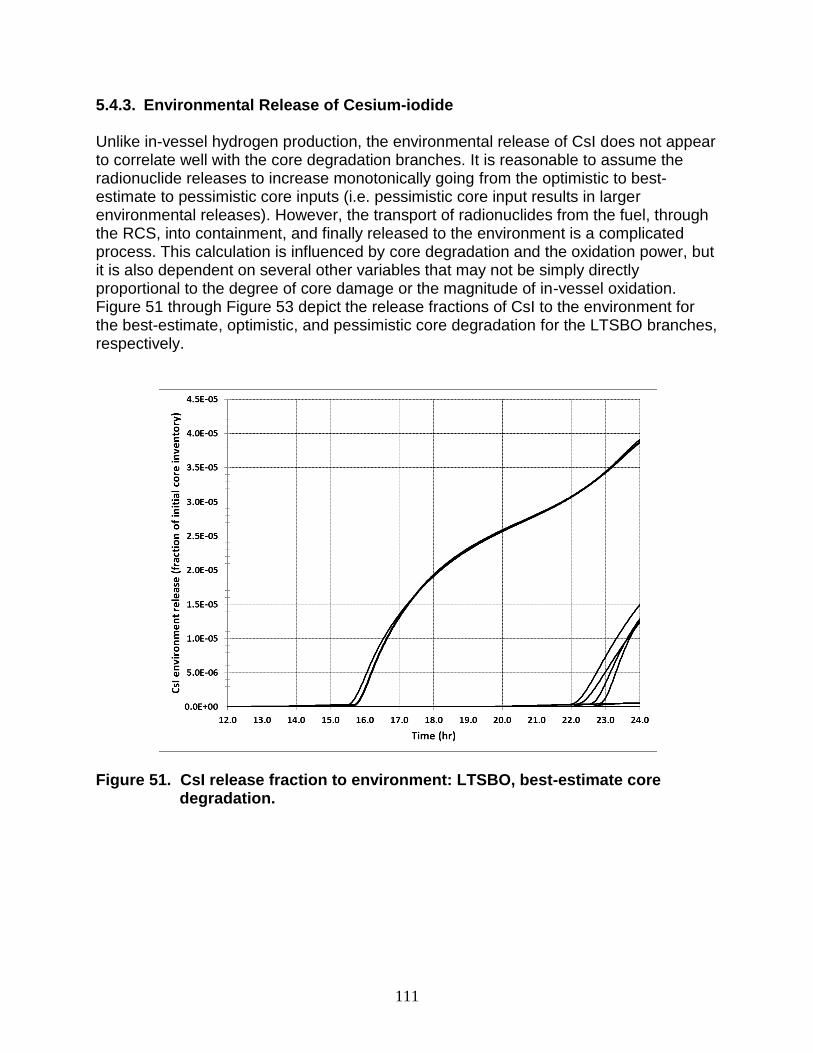
111

5.4.3. Environmental Release of Cesium-iodide

Unlike in-vessel hydrogen production, the environmental release of CsI does not appear to correlate well with the core degradation branches. It is reasonable to assume the radionuclide releases to increase monotonically going from the optimistic to best-estimate to pessimistic core inputs (i.e. pessimistic core input results in larger environmental releases). However, the transport of radionuclides from the fuel, through the RCS, into containment, and finally released to the environment is a complicated process. This calculation is influenced by core degradation and the oxidation power, but it is also dependent on several other variables that may not be simply directly proportional to the degree of core damage or the magnitude of in-vessel oxidation. Figure 51 through Figure 53 depict the release fractions of CsI to the environment for the best-estimate, optimistic, and pessimistic core degradation for the LTSBO branches, respectively.

Figure 51. CsI release fraction to environment: LTSBO, best-estimate core

degradation.

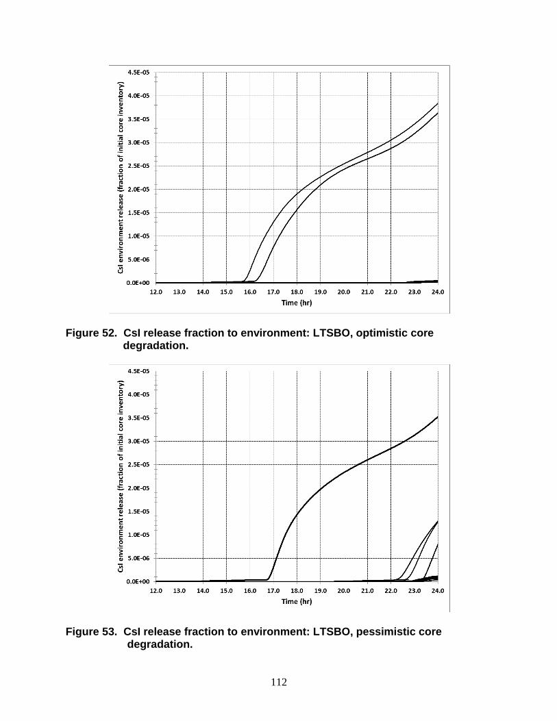
112

Figure 52. CsI release fraction to environment: LTSBO, optimistic core

degradation.

Figure 53. CsI release fraction to environment: LTSBO, pessimistic core

degradation.

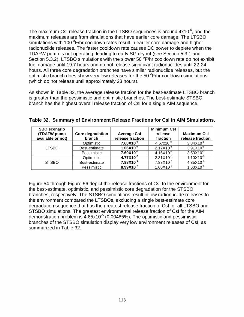
113

The maximum CsI release fraction in the LTSBO sequences is around 4x10-5, and the maximum releases are from simulations that have earlier core damage. The LTSBO simulations with 100 oF/hr cooldown rates result in earlier core damage and higher radionuclide releases. The faster cooldown rate causes DC power to deplete when the TDAFW pump is not operating, leading to early SG dryout (see Section 5.3.1 and Section 5.3.2). LTSBO simulations with the slower 50 oF/hr cooldown rate do not exhibit fuel damage until 19.7 hours and do not release significant radionuclides until 22-24 hours. All three core degradation branches have similar radionuclide releases, but the optimistic branch does show very low releases for the 50 oF/hr cooldown simulations (which do not release until approximately 23 hours). As shown in Table 32, the average release fraction for the best-estimate LTSBO branch is greater than the pessimistic and optimistic branches. The best-estimate STSBO branch has the highest overall release fraction of CsI for a single AIM sequence.

Table 32. Summary of Environment Release Fractions for CsI in AIM Simulations.

SBO scenario (TDAFW pump

available or not) Core degradation

branch Average CsI

release fraction

Minimum CsI release fraction

Maximum CsI release fraction

LTSBO

Optimistic 7.68X10-6

4.67x10-8

3.84X10-5

Best-estimate 1.06X10-5

2.17X10-8

3.91X10-5

Pessimistic 7.60X10-6

4.16X10-7

3.53X10-5

STSBO

Optimistic 4.77X10-7

2.31X10-8

1.10X10-6

Best-estimate 7.88X10-6

7.88X10-7

4.85X10-5

Pessimistic 8.99X10-7

1.60X10-8

1.60X10-6

Figure 54 through Figure 56 depict the release fractions of CsI to the environment for the best-estimate, optimistic, and pessimistic core degradation for the STSBO branches, respectively. The STSBO simulations result in low radionuclide releases to the environment compared the LTSBOs, excluding a single best-estimate core degradation sequence that has the greatest release fraction of CsI for all LTSBO and STSBO simulations. The greatest environmental release fraction of CsI for the AIM demonstration problem is 4.85x10-5 (0.00485%). The optimistic and pessimistic branches of the STSBO simulation display very low environment releases of CsI, as summarized in Table 32.

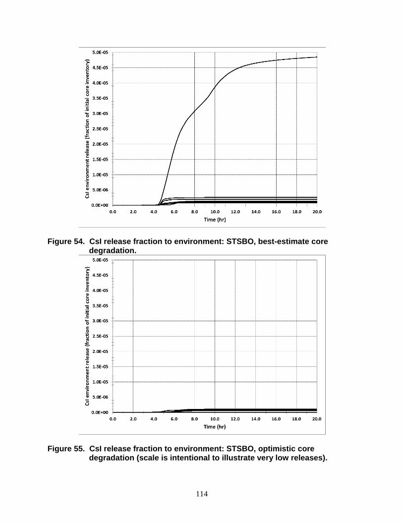
114

Figure 54. CsI release fraction to environment: STSBO, best-estimate core

degradation.

Figure 55. CsI release fraction to environment: STSBO, optimistic core

degradation (scale is intentional to illustrate very low releases).

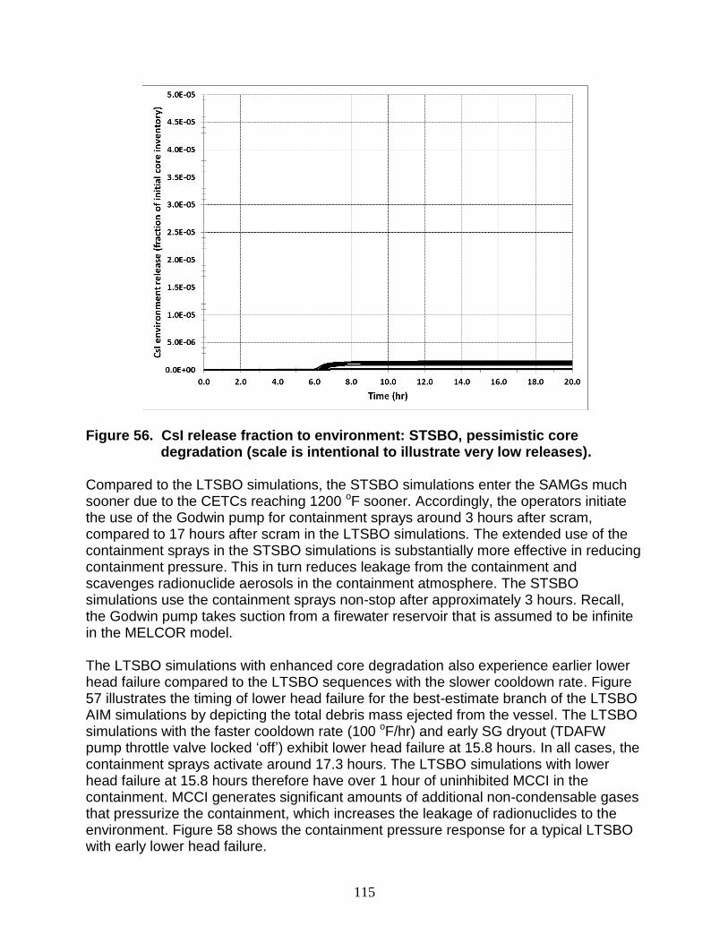
115

Figure 56. CsI release fraction to environment: STSBO, pessimistic core

degradation (scale is intentional to illustrate very low releases).

Compared to the LTSBO simulations, the STSBO simulations enter the SAMGs much sooner due to the CETCs reaching 1200 oF sooner. Accordingly, the operators initiate the use of the Godwin pump for containment sprays around 3 hours after scram, compared to 17 hours after scram in the LTSBO simulations. The extended use of the containment sprays in the STSBO simulations is substantially more effective in reducing containment pressure. This in turn reduces leakage from the containment and scavenges radionuclide aerosols in the containment atmosphere. The STSBO simulations use the containment sprays non-stop after approximately 3 hours. Recall, the Godwin pump takes suction from a firewater reservoir that is assumed to be infinite in the MELCOR model. The LTSBO simulations with enhanced core degradation also experience earlier lower head failure compared to the LTSBO sequences with the slower cooldown rate. Figure 57 illustrates the timing of lower head failure for the best-estimate branch of the LTSBO AIM simulations by depicting the total debris mass ejected from the vessel. The LTSBO simulations with the faster cooldown rate (100 oF/hr) and early SG dryout (TDAFW pump throttle valve locked ‘off’) exhibit lower head failure at 15.8 hours. In all cases, the containment sprays activate around 17.3 hours. The LTSBO simulations with lower head failure at 15.8 hours therefore have over 1 hour of uninhibited MCCI in the containment. MCCI generates significant amounts of additional non-condensable gases that pressurize the containment, which increases the leakage of radionuclides to the environment. Figure 58 shows the containment pressure response for a typical LTSBO with early lower head failure.

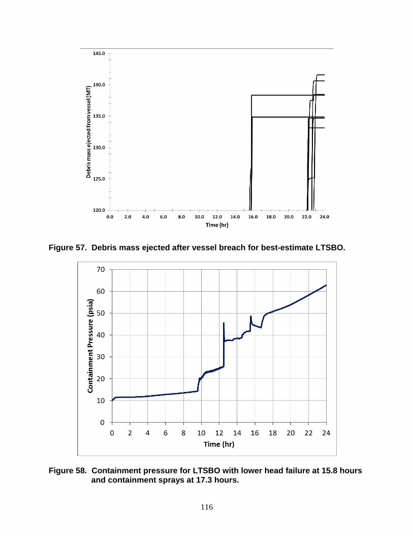
116

Figure 57. Debris mass ejected after vessel breach for best-estimate LTSBO.

Figure 58. Containment pressure for LTSBO with lower head failure at 15.8 hours

and containment sprays at 17.3 hours.

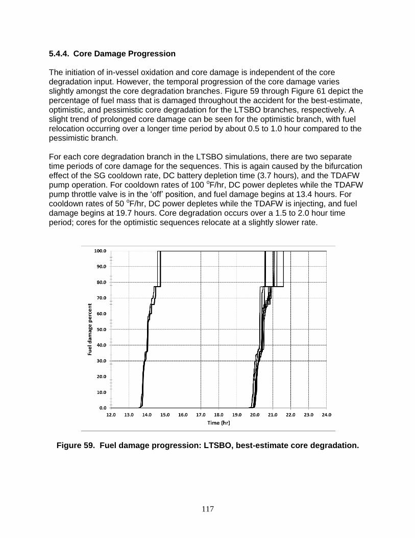
117

5.4.4. Core Damage Progression The initiation of in-vessel oxidation and core damage is independent of the core degradation input. However, the temporal progression of the core damage varies slightly amongst the core degradation branches. Figure 59 through Figure 61 depict the percentage of fuel mass that is damaged throughout the accident for the best-estimate, optimistic, and pessimistic core degradation for the LTSBO branches, respectively. A slight trend of prolonged core damage can be seen for the optimistic branch, with fuel relocation occurring over a longer time period by about 0.5 to 1.0 hour compared to the pessimistic branch. For each core degradation branch in the LTSBO simulations, there are two separate time periods of core damage for the sequences. This is again caused by the bifurcation effect of the SG cooldown rate, DC battery depletion time (3.7 hours), and the TDAFW pump operation. For cooldown rates of 100 oF/hr, DC power depletes while the TDAFW pump throttle valve is in the ‘off’ position, and fuel damage begins at 13.4 hours. For cooldown rates of 50 oF/hr, DC power depletes while the TDAFW is injecting, and fuel damage begins at 19.7 hours. Core degradation occurs over a 1.5 to 2.0 hour time period; cores for the optimistic sequences relocate at a slightly slower rate.

Figure 59. Fuel damage progression: LTSBO, best-estimate core degradation.

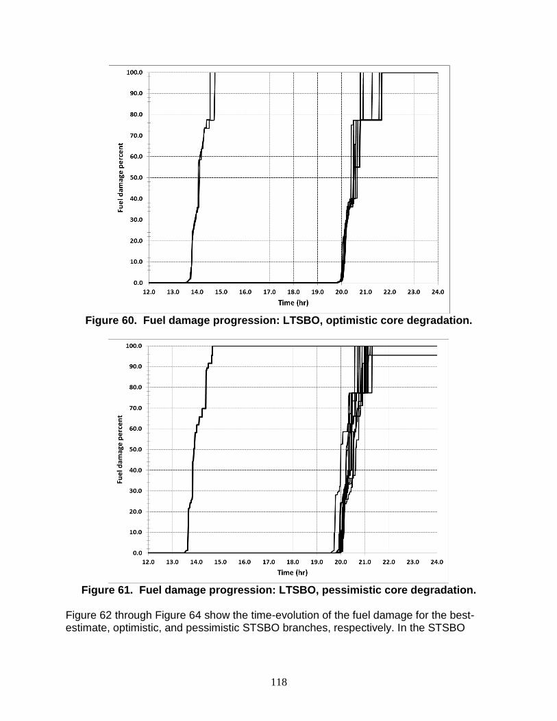
118

Figure 60. Fuel damage progression: LTSBO, optimistic core degradation.

Figure 61. Fuel damage progression: LTSBO, pessimistic core degradation.

Figure 62 through Figure 64 show the time-evolution of the fuel damage for the best-estimate, optimistic, and pessimistic STSBO branches, respectively. In the STSBO

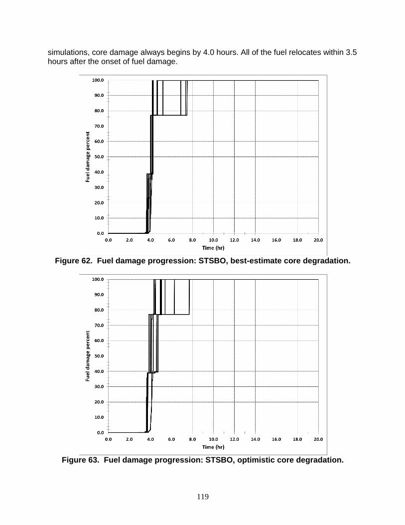
119

simulations, core damage always begins by 4.0 hours. All of the fuel relocates within 3.5 hours after the onset of fuel damage.

Figure 62. Fuel damage progression: STSBO, best-estimate core degradation.

Figure 63. Fuel damage progression: STSBO, optimistic core degradation.

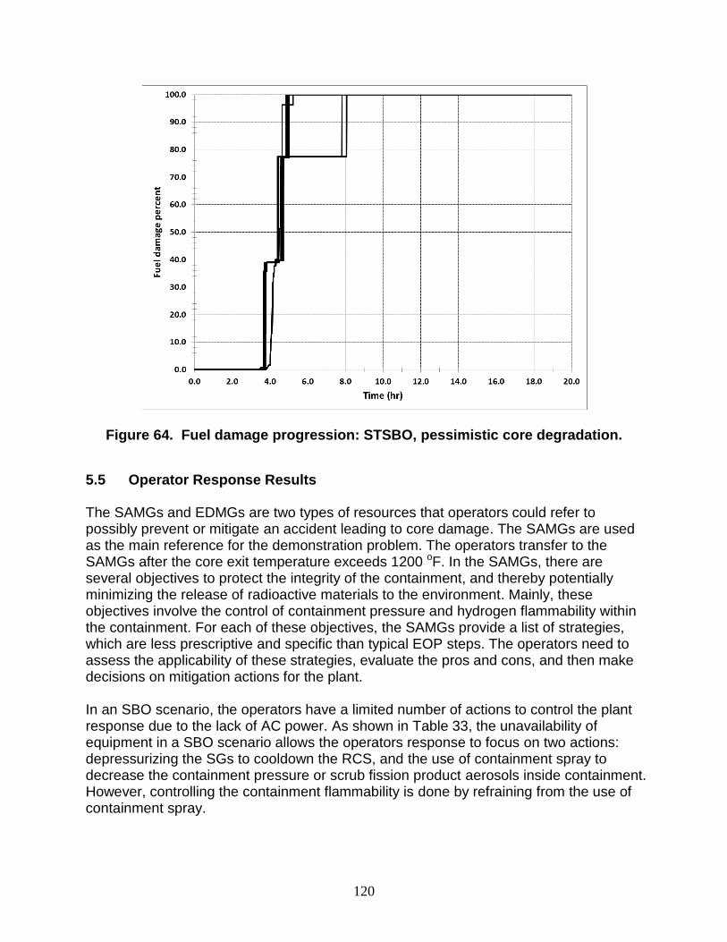
120

Figure 64. Fuel damage progression: STSBO, pessimistic core degradation.

5.5 Operator Response Results

The SAMGs and EDMGs are two types of resources that operators could refer to possibly prevent or mitigate an accident leading to core damage. The SAMGs are used as the main reference for the demonstration problem. The operators transfer to the SAMGs after the core exit temperature exceeds 1200 oF. In the SAMGs, there are several objectives to protect the integrity of the containment, and thereby potentially minimizing the release of radioactive materials to the environment. Mainly, these objectives involve the control of containment pressure and hydrogen flammability within the containment. For each of these objectives, the SAMGs provide a list of strategies, which are less prescriptive and specific than typical EOP steps. The operators need to assess the applicability of these strategies, evaluate the pros and cons, and then make decisions on mitigation actions for the plant. In an SBO scenario, the operators have a limited number of actions to control the plant response due to the lack of AC power. As shown in Table 33, the unavailability of equipment in a SBO scenario allows the operators response to focus on two actions: depressurizing the SGs to cooldown the RCS, and the use of containment spray to decrease the containment pressure or scrub fission product aerosols inside containment. However, controlling the containment flammability is done by refraining from the use of containment spray.

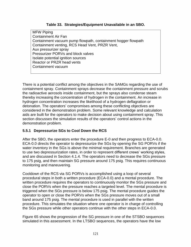
121

Table 33. Strategies/Equipment Unavailable in an SBO.

MFW Piping Containment Air Fan Containment vacuum pump flowpath, containment hogger flowpath Containment venting, RCS Head Vent, PRZR Vent, Aux pressurizer spray Pressurizer PORVs and block valves Isolate potential ignition sources Reactor or PRZR head vents Containment vacuum

There is a potential conflict among the objectives in the SAMGs regarding the use of containment spray. Containment sprays decrease the containment pressure and scrubs the radioactive aerosols inside containment, but the sprays also condense steam thereby increasing the concentration of hydrogen in the containment. An increase in hydrogen concentration increases the likelihood of a hydrogen deflagration or detonation. The operators’ compromises among these conflicting objectives are considered in the demonstration problem. Some relevant knowledge and calculation aids are built for the operators to make decision about using containment spray. This section discusses the simulation results of the operators’ control actions in the demonstration problem.

5.5.1 Depressurize SGs to Cool Down the RCS

After the SBO, the operators enter the procedure E-0 and then progress to ECA-0.0. ECA-0.0 directs the operator to depressurize the SGs by opening the SG PORVs if the water inventory in the SGs is above the minimal requirement. Branches are generated to use two depressurization rates, in order to represent different crews’ working styles, and are discussed in Section 4.1.4. The operators need to decrease the SGs pressure to 175 psig, and then maintain SG pressure around 175 psig. This requires continuous monitoring and maneuvering. Cooldown of the RCS via SG PORVs is accomplished using a loop of several procedural steps in both a written procedure (ECA-0.0) and a mental procedure. The written procedure requires the operators to continuously monitor the SGs pressure and close the PORVs when the pressure reaches a targeted level. The mental procedure is triggered when the SGs pressure is below 175 psig. The mental procedure guides the operator to open or close the PORVs when the SGs pressure moves out of a small band around 175 psig. The mental procedure is used in parallel with the written procedure. This simulates the situation where one operator is in charge of controlling the SGs pressure while other operators continue with the other steps in ECA-0.0. Figure 65 shows the progression of the SG pressure in one of the STSBO sequences simulated in this assessment. In the LTSBO sequences, the operators have the low

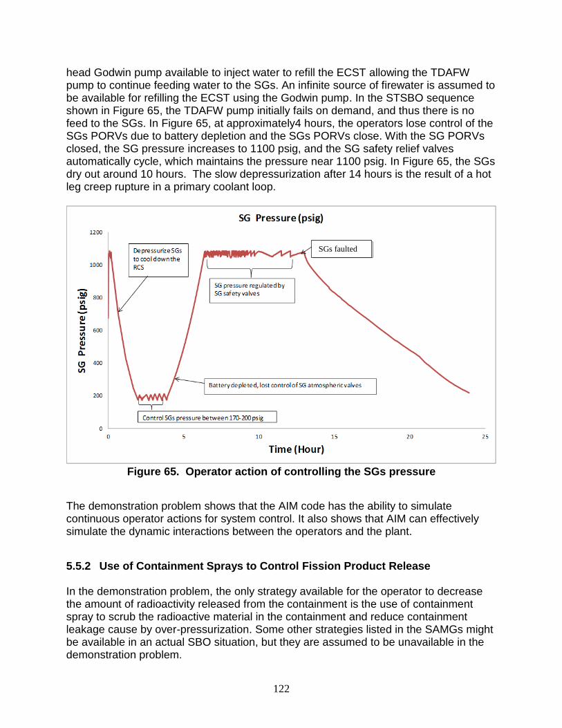
122

head Godwin pump available to inject water to refill the ECST allowing the TDAFW pump to continue feeding water to the SGs. An infinite source of firewater is assumed to be available for refilling the ECST using the Godwin pump. In the STSBO sequence shown in Figure 65, the TDAFW pump initially fails on demand, and thus there is no feed to the SGs. In Figure 65, at approximately4 hours, the operators lose control of the SGs PORVs due to battery depletion and the SGs PORVs close. With the SG PORVs closed, the SG pressure increases to 1100 psig, and the SG safety relief valves automatically cycle, which maintains the pressure near 1100 psig. In Figure 65, the SGs dry out around 10 hours. The slow depressurization after 14 hours is the result of a hot leg creep rupture in a primary coolant loop.

Figure 65. Operator action of controlling the SGs pressure

The demonstration problem shows that the AIM code has the ability to simulate continuous operator actions for system control. It also shows that AIM can effectively simulate the dynamic interactions between the operators and the plant.

5.5.2 Use of Containment Sprays to Control Fission Product Release

In the demonstration problem, the only strategy available for the operator to decrease the amount of radioactivity released from the containment is the use of containment spray to scrub the radioactive material in the containment and reduce containment leakage cause by over-pressurization. Some other strategies listed in the SAMGs might be available in an actual SBO situation, but they are assumed to be unavailable in the demonstration problem.

SGs faulted

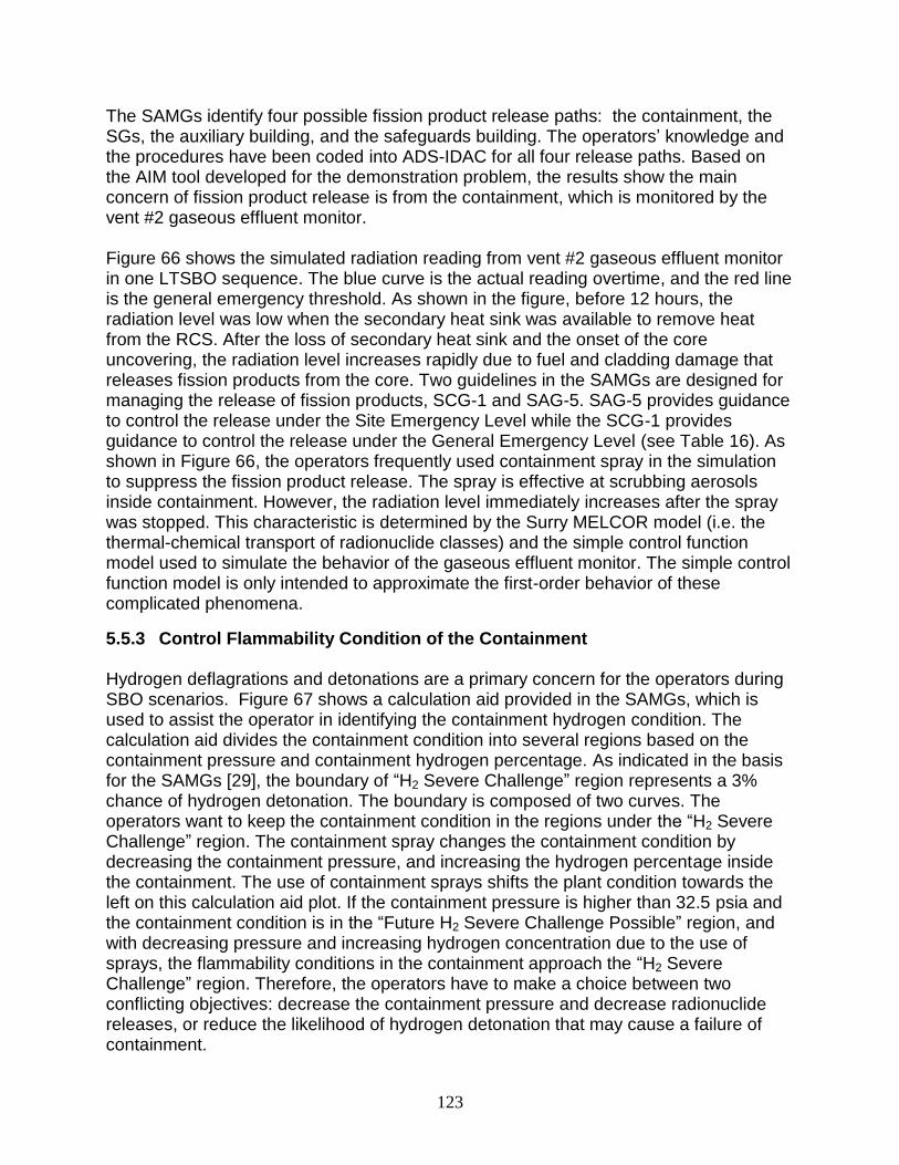
123

The SAMGs identify four possible fission product release paths: the containment, the SGs, the auxiliary building, and the safeguards building. The operators’ knowledge and the procedures have been coded into ADS-IDAC for all four release paths. Based on the AIM tool developed for the demonstration problem, the results show the main concern of fission product release is from the containment, which is monitored by the vent #2 gaseous effluent monitor. Figure 66 shows the simulated radiation reading from vent #2 gaseous effluent monitor in one LTSBO sequence. The blue curve is the actual reading overtime, and the red line is the general emergency threshold. As shown in the figure, before 12 hours, the radiation level was low when the secondary heat sink was available to remove heat from the RCS. After the loss of secondary heat sink and the onset of the core uncovering, the radiation level increases rapidly due to fuel and cladding damage that releases fission products from the core. Two guidelines in the SAMGs are designed for managing the release of fission products, SCG-1 and SAG-5. SAG-5 provides guidance to control the release under the Site Emergency Level while the SCG-1 provides guidance to control the release under the General Emergency Level (see Table 16). As shown in Figure 66, the operators frequently used containment spray in the simulation to suppress the fission product release. The spray is effective at scrubbing aerosols inside containment. However, the radiation level immediately increases after the spray was stopped. This characteristic is determined by the Surry MELCOR model (i.e. the thermal-chemical transport of radionuclide classes) and the simple control function model used to simulate the behavior of the gaseous effluent monitor. The simple control function model is only intended to approximate the first-order behavior of these complicated phenomena.

5.5.3 Control Flammability Condition of the Containment

Hydrogen deflagrations and detonations are a primary concern for the operators during SBO scenarios. Figure 67 shows a calculation aid provided in the SAMGs, which is used to assist the operator in identifying the containment hydrogen condition. The calculation aid divides the containment condition into several regions based on the containment pressure and containment hydrogen percentage. As indicated in the basis for the SAMGs [29], the boundary of “H2 Severe Challenge” region represents a 3% chance of hydrogen detonation. The boundary is composed of two curves. The operators want to keep the containment condition in the regions under the “H2 Severe Challenge” region. The containment spray changes the containment condition by decreasing the containment pressure, and increasing the hydrogen percentage inside the containment. The use of containment sprays shifts the plant condition towards the left on this calculation aid plot. If the containment pressure is higher than 32.5 psia and the containment condition is in the “Future H2 Severe Challenge Possible” region, and with decreasing pressure and increasing hydrogen concentration due to the use of sprays, the flammability conditions in the containment approach the “H2 Severe Challenge” region. Therefore, the operators have to make a choice between two conflicting objectives: decrease the containment pressure and decrease radionuclide releases, or reduce the likelihood of hydrogen detonation that may cause a failure of containment.

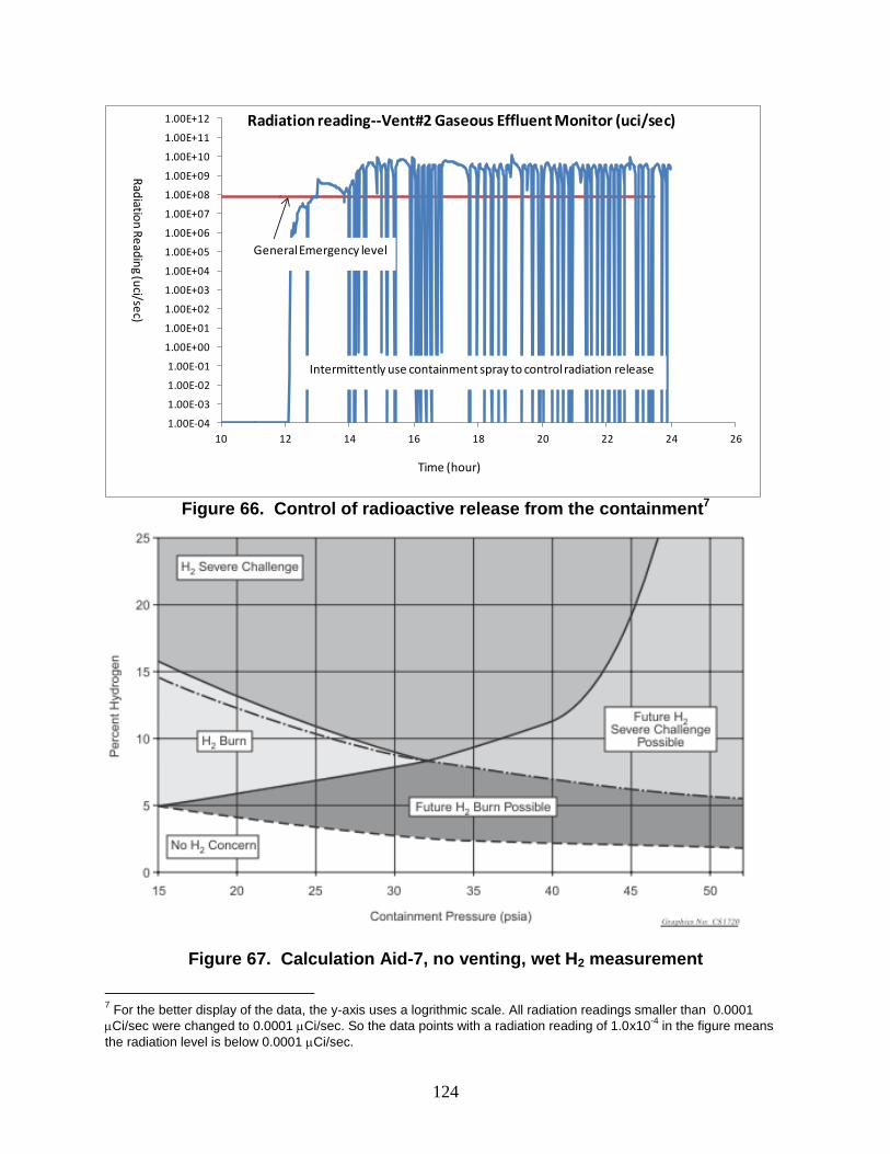
124

Figure 66. Control of radioactive release from the containment7

Figure 67. Calculation Aid-7, no venting, wet H2 measurement

7 For the better display of the data, the y-axis uses a logrithmic scale. All radiation readings smaller than 0.0001

Ci/sec were changed to 0.0001 Ci/sec. So the data points with a radiation reading of 1.0x10-4

in the figure means

the radiation level is below 0.0001 Ci/sec.

1.00E-04

1.00E-03

1.00E-02

1.00E-01

1.00E+00

1.00E+01

1.00E+02

1.00E+03

1.00E+04

1.00E+05

1.00E+06

1.00E+07

1.00E+08

1.00E+09

1.00E+10

1.00E+11

1.00E+12

10 12 14 16 18 20 22 24 26

Radiation reading--Vent#2 Gaseous Effluent Monitor (uci/sec)

General Emergency level

Intermittently use containment spray to control radiation release

Time (hour)

Rad

iation

Re

adin

g (uci/se

c)

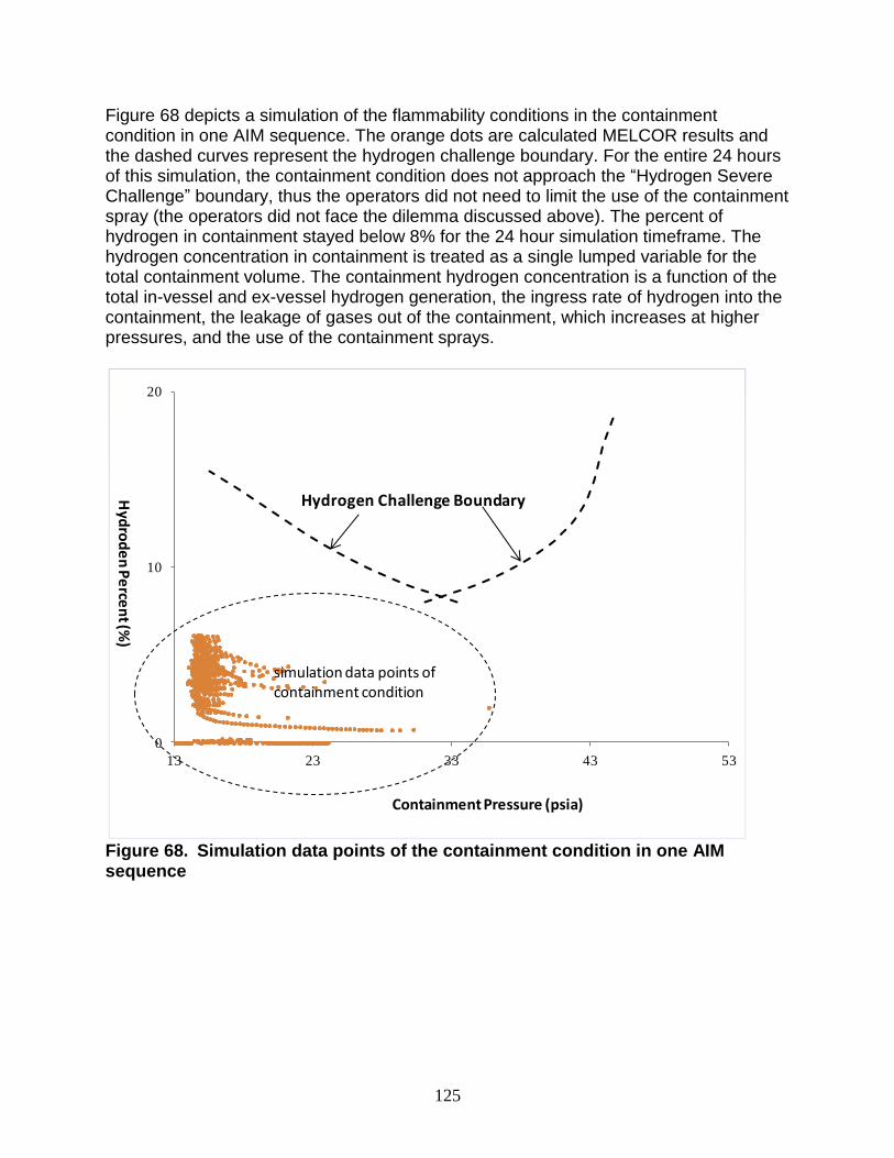
125

Figure 68 depicts a simulation of the flammability conditions in the containment condition in one AIM sequence. The orange dots are calculated MELCOR results and the dashed curves represent the hydrogen challenge boundary. For the entire 24 hours of this simulation, the containment condition does not approach the “Hydrogen Severe Challenge” boundary, thus the operators did not need to limit the use of the containment spray (the operators did not face the dilemma discussed above). The percent of hydrogen in containment stayed below 8% for the 24 hour simulation timeframe. The hydrogen concentration in containment is treated as a single lumped variable for the total containment volume. The containment hydrogen concentration is a function of the total in-vessel and ex-vessel hydrogen generation, the ingress rate of hydrogen into the containment, the leakage of gases out of the containment, which increases at higher pressures, and the use of the containment sprays.

Figure 68. Simulation data points of the containment condition in one AIM sequence

0

10

20

13 23 33 43 53

Containment Pressure (psia)

Hyd

rod

en

Pe

rcen

t (%)

Hydrogen Challenge Boundary

simulation data points of containment condition

126

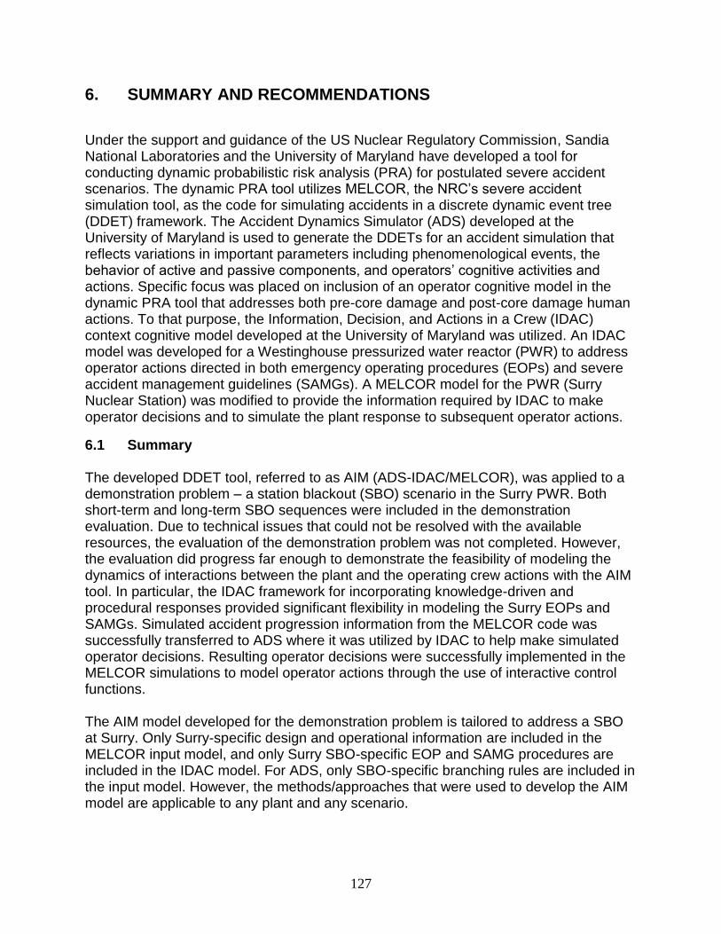
127

6. SUMMARY AND RECOMMENDATIONS

Under the support and guidance of the US Nuclear Regulatory Commission, Sandia National Laboratories and the University of Maryland have developed a tool for conducting dynamic probabilistic risk analysis (PRA) for postulated severe accident scenarios. The dynamic PRA tool utilizes MELCOR, the NRC’s severe accident simulation tool, as the code for simulating accidents in a discrete dynamic event tree (DDET) framework. The Accident Dynamics Simulator (ADS) developed at the University of Maryland is used to generate the DDETs for an accident simulation that reflects variations in important parameters including phenomenological events, the behavior of active and passive components, and operators’ cognitive activities and actions. Specific focus was placed on inclusion of an operator cognitive model in the dynamic PRA tool that addresses both pre-core damage and post-core damage human actions. To that purpose, the Information, Decision, and Actions in a Crew (IDAC) context cognitive model developed at the University of Maryland was utilized. An IDAC model was developed for a Westinghouse pressurized water reactor (PWR) to address operator actions directed in both emergency operating procedures (EOPs) and severe accident management guidelines (SAMGs). A MELCOR model for the PWR (Surry Nuclear Station) was modified to provide the information required by IDAC to make operator decisions and to simulate the plant response to subsequent operator actions.

6.1 Summary The developed DDET tool, referred to as AIM (ADS-IDAC/MELCOR), was applied to a demonstration problem – a station blackout (SBO) scenario in the Surry PWR. Both short-term and long-term SBO sequences were included in the demonstration evaluation. Due to technical issues that could not be resolved with the available resources, the evaluation of the demonstration problem was not completed. However, the evaluation did progress far enough to demonstrate the feasibility of modeling the dynamics of interactions between the plant and the operating crew actions with the AIM tool. In particular, the IDAC framework for incorporating knowledge-driven and procedural responses provided significant flexibility in modeling the Surry EOPs and SAMGs. Simulated accident progression information from the MELCOR code was successfully transferred to ADS where it was utilized by IDAC to help make simulated operator decisions. Resulting operator decisions were successfully implemented in the MELCOR simulations to model operator actions through the use of interactive control functions. The AIM model developed for the demonstration problem is tailored to address a SBO at Surry. Only Surry-specific design and operational information are included in the MELCOR input model, and only Surry SBO-specific EOP and SAMG procedures are included in the IDAC model. For ADS, only SBO-specific branching rules are included in the input model. However, the methods/approaches that were used to develop the AIM model are applicable to any plant and any scenario.

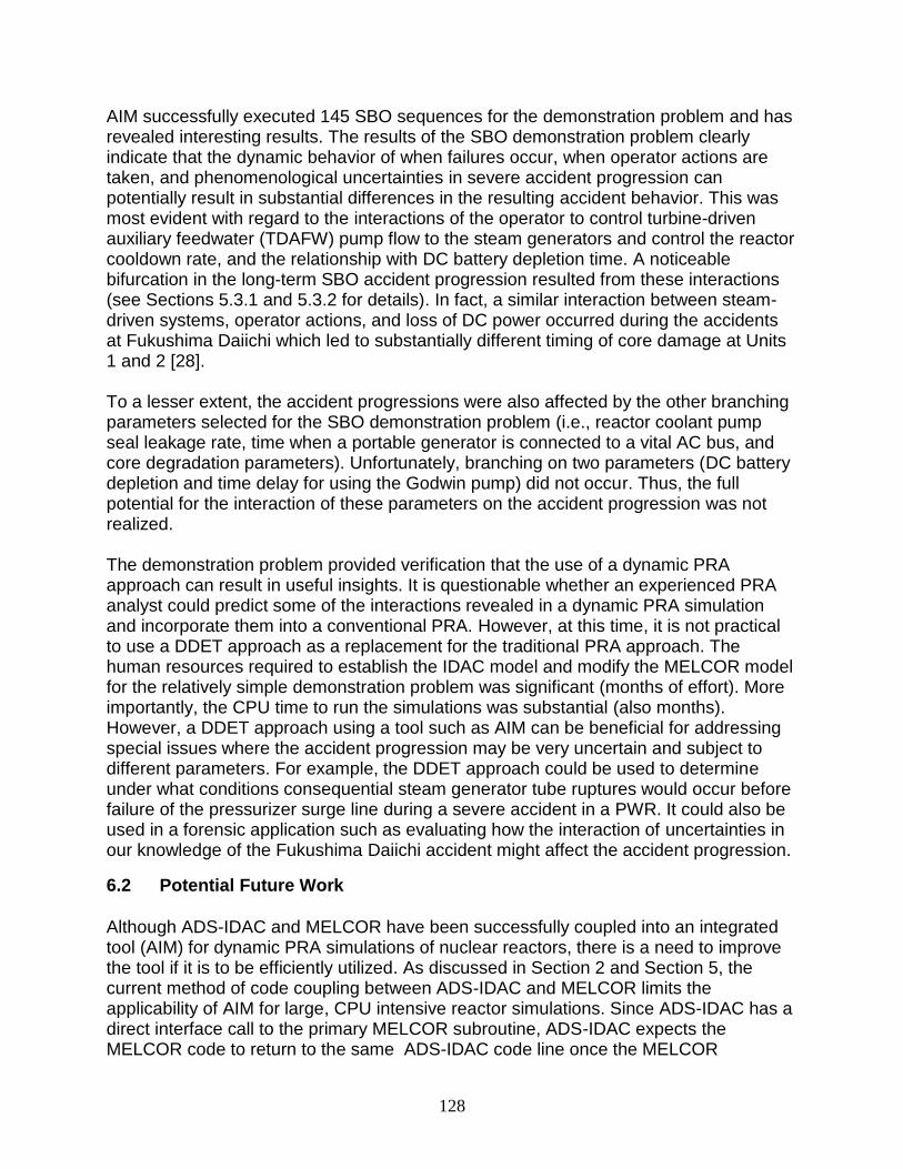
128

AIM successfully executed 145 SBO sequences for the demonstration problem and has revealed interesting results. The results of the SBO demonstration problem clearly indicate that the dynamic behavior of when failures occur, when operator actions are taken, and phenomenological uncertainties in severe accident progression can potentially result in substantial differences in the resulting accident behavior. This was most evident with regard to the interactions of the operator to control turbine-driven auxiliary feedwater (TDAFW) pump flow to the steam generators and control the reactor cooldown rate, and the relationship with DC battery depletion time. A noticeable bifurcation in the long-term SBO accident progression resulted from these interactions (see Sections 5.3.1 and 5.3.2 for details). In fact, a similar interaction between steam-driven systems, operator actions, and loss of DC power occurred during the accidents at Fukushima Daiichi which led to substantially different timing of core damage at Units 1 and 2 [28]. To a lesser extent, the accident progressions were also affected by the other branching parameters selected for the SBO demonstration problem (i.e., reactor coolant pump seal leakage rate, time when a portable generator is connected to a vital AC bus, and core degradation parameters). Unfortunately, branching on two parameters (DC battery depletion and time delay for using the Godwin pump) did not occur. Thus, the full potential for the interaction of these parameters on the accident progression was not realized. The demonstration problem provided verification that the use of a dynamic PRA approach can result in useful insights. It is questionable whether an experienced PRA analyst could predict some of the interactions revealed in a dynamic PRA simulation and incorporate them into a conventional PRA. However, at this time, it is not practical to use a DDET approach as a replacement for the traditional PRA approach. The human resources required to establish the IDAC model and modify the MELCOR model for the relatively simple demonstration problem was significant (months of effort). More importantly, the CPU time to run the simulations was substantial (also months). However, a DDET approach using a tool such as AIM can be beneficial for addressing special issues where the accident progression may be very uncertain and subject to different parameters. For example, the DDET approach could be used to determine under what conditions consequential steam generator tube ruptures would occur before failure of the pressurizer surge line during a severe accident in a PWR. It could also be used in a forensic application such as evaluating how the interaction of uncertainties in our knowledge of the Fukushima Daiichi accident might affect the accident progression.

6.2 Potential Future Work

Although ADS-IDAC and MELCOR have been successfully coupled into an integrated tool (AIM) for dynamic PRA simulations of nuclear reactors, there is a need to improve the tool if it is to be efficiently utilized. As discussed in Section 2 and Section 5, the current method of code coupling between ADS-IDAC and MELCOR limits the applicability of AIM for large, CPU intensive reactor simulations. Since ADS-IDAC has a direct interface call to the primary MELCOR subroutine, ADS-IDAC expects the MELCOR code to return to the same ADS-IDAC code line once the MELCOR

129

simulation has completely finished either due to reaching the simulation truncation time or due to MELCOR experiencing an error. Upon returning to this line in ADS-IDAC, the code continues to execute any remaining queued sequences. Unfortunately, when MELCOR encounters an error it will not return to ADS-IDAC properly; it exits via a Fortran ‘call exit()’ statement, which terminates the entire AIM simulation since it is a single application (i.e. an integrated executable). In hindsight, an externally coupled tool would have been more resilient to MELCOR error issues, which would have facilitated the simulation of the demonstration problem. For example, a “master” script could execute both ADS-IDAC and MELCOR independently, exchanging data through text/binary files or a common socket. Barring any major code rewrites to MELCOR 2.1, an external code coupling method is probably the most practical technique for performing dynamic PRA simulations with MELCOR. This approach is currently utilized in using ADAPT with MELCOR to run dynamic PRA simulations8. It should be noted that numerous temporary fixes to the MELCOR ‘call exit()’ issue were attempted for the AIM model. Because MELCOR calls the ‘call exit()’ subroutine from various locations in the code, many of which are within several nested subroutines, this issue could not be alleviated by a simple or temporary solution. If the ‘call exit()’ statement is merely avoided, the subroutines detecting an error never expect the code to return after attempting to terminate the application, and there is no further error-checking logic that prevents the code from attempting to continue the simulation. Thus, MELCOR will continue in an error state and inevitably encounter a run-time error if it does not terminate via ‘call exit().’ In order to have an internally coupled ADS-IDAC and MELCOR code for PRA calculations, significant revisions are required in the MELCOR source code that are beyond the current scope of this research. Future research in dynamic PRA with AIM should first focus on reducing the integrated coupling scheme to a simpler and more resilient external coupling technique. If MELCOR and ADS-IDAC are separate, ADS-IDAC would not be affected by MELCOR errors and could easily recover additional queued sequences after MELCOR encounters an error. A simple and fast-running MELCOR demonstration model should be developed to demonstrate the external coupling with the serial version of ADS-IDAC (i.e. a few dozen sequences). Next, the externally-coupled AIM tool should be expanded to the multi-processor version of ADS-IDAC. In order to keep CPU time reasonable for long-running severe accident simulations (i.e., approximately 105 seconds) and for hundreds of sequences, it is imperative to take advantage of multi-core processing on modern computer clusters. Development of the input models for such a large dynamic PRA simulation requires an iterative debugging method, which would be necessary for developing input for any code. Run-times in excess of several weeks are not conducive for the input development for new models and new codes.

8 Using ADAPT within this phase of the project was investigated early on, but the resource projections developed

by the contributors exceeded what the project could support.

130

Several new features were recently incorporated into ADS-IDAC/RELAP5 that should eventually be ported to AIM. Although these features do not address the MELCOR ‘call exit()’ issue, they would drastically decrease the resources required to develop ADS-IDAC and MELCOR input for future AIM applications. The most important new features include:

1. The capability to restart ADS-IDAC. Recently, the multiprocessor version of ADS-IDAC/RELAP5 was given the ability to restart the coupled simulation from a particular point in time and from a particular sequence. Incorporating this feature into AIM would drastically decrease the time required to develop and debug ADS-IDAC and MELCOR input. Currently, AIM requires an ad-hoc and time-consuming scheme to perform pseudo-restarts in order to debug certain parts of code input.

2. The ADS graphical user interface (GUI) has improved capabilities in performing input-format checking of procedure input files, which includes detecting format errors and providing a user-friendly interface to guide the user in resolving the procedure input errors. Currently, the development and debugging of the procedure input files for AIM is a very tedious and time-consuming process, as described in Section 2.4.4. For future AIM applications, input procedure files for ADS-IDAC could be debugged using the ADS GUI for detecting input format errors.

In addition to these ADS-IDAC features, it would be desirable to improve the method for encoding operator procedures. Currently, this is not very user friendly. Beyond modifications to the AIM tool, incorporation of ADAPT in to the framework shown in Figure 3 could be pursued. The use of ADAPT for scheduling, process control, and sequence tracking would alleviate some of the issues that need to be addressed with AIM. However, an interface between ADS-IDAC and ADAPT would have to be developed in this framework. Reference 16 provides the suggested steps necessary for the integration of ADS-IDAC, ADAPT, and MELCOR. In addition, recent developments with ADAPT (e.g., post-processing capability) could be pursued in this effort.

131

7. REFERENCES

1. “Agency Long-Term Research Activities for Fiscal Year 2009,” SECY-07-0192, U.S. Nuclear Regulatory Commission, 31 October 2007. Available via the US NRC’s Agencywide Document Access and Management System (ADAMS) at accession no. ML072780393.

2. D. Helton, “Scoping Study on Advancing Modeling Techniques for Level 2/3 PRA,” U.S. Nuclear Regulatory Commission, May 2009. Available via the US NRC’s Agencywide Document Access and Management System (ADAMS) at accession no. ML091320454.

3. Richard Chang, et al., “State-of-the-Art Reactor Consequences Analyses (SOARCA) Report: Draft Report for Comment,” NUREG-1935, US Nuclear Regulatory Commission, January 2012.

4. D. Kunsman, et.al, “Development and Application of the Dynamic System Doctor to Nuclear Reactor Probabilistic Risk Assessments,” SAND2008-4746, Sandia National Laboratories, May 2008.

5. A. Hakobyan, et al., “Dynamic Generation of Accident Progression Event Trees,” A. Nuclear Engineering & Design, Volume 238, Issue 12, pg. 3457-3467.

6. Sandia National Laboratories, “MELCOR Computer Code Manuals,” Version 2.1, DRAFT (2012).

7. B. Rutt, et al., “Distributed dynamic event tree generation for reliability and risk assessment, Challenges of Large Applications in Distributed Environments,” 2006 IEEE , vol., no., pp.61-70.

8. Y. H. J. Chang and A. Mosleh, “Cognitive modeling and dynamic probabilistic simulation of operating crew response to complex system accidents. Part 5: Dynamic probabilistic simulation of the IDAC model,” Reliability Engineering and System Safety 92 (2007) pp 1076-1101.

9. Y. H. J. Chang and A. Mosleh, “Cognitive modeling and dynamic probabilistic simulation of operating crew response to complex system accidents. Part 1: Overview of the IDAC model,” Reliability Engineering and System Safety 92 (2007) pp 997-1013.

10. K.A Coyne and A. Mosleh, “Modeling nuclear plant operator knowledge and actions - the ads-idac simulation approach”, ANS PSA 2008 Topical Meeting-Challenges to PSA during the nuclear renaissance. Knoxville, Tennessee, 2008.

11. K.A. Coyne, and A. Mosleh, “Implementation of a Dynamic PRA Approach for the Prediction of Operator Errors During Abnormal Nuclear Power Plant Events”, 9th

132

International Probabilistic Safety Assessment and Management Conference, Hong Kong, 2008.

12. M. Kloss and J. Preschke, “MCDET- A Probabilistic Dynamics Method Combining Monte Carlo Simulation with the Discrete Dynamic Event Tree Approach,” Nuclear Science and Engineering 153, pg. 137-156.

13. J. Preschke and M. Kloss, “Impact of Epistemic Uncertainties on the Probabilistic Assessment of the Emergency Operating Procedure Secondary Side Bleed and Feed”, 9th International Probabilistic Safety Assessment and Management Conference, Hong Kong, China (May 18-23).

14. J. Preschke and M. Kloss, “Analysis of Human Actions in the Framework of Dynamic Reliability Analysis,” 8th International Probabilistic Safety Assessment and Management Conference, New Orleans, Louisiana, USA (May 14-18).

15. J. LaChance, R. Boring, J. Danneels, C. Hansen, N. Bixler, and R. Gauntt, “Review of Scoping Study on Advancing Modeling Techniques for Level 2/3 PRA, Task 1 Letter Report,” JCN N6780 Letter Report, Sandia National Laboratories, October 18, 2009.

16. J. LaChance, et al., “Advancing Modeling Techniques for Level 2/3 PRA – Methodology Development Plan,” Letter Report, Sandia National Laboratory, January 11, 2011.

17. K. Metzroth, R. Denning, C. Smidts, and T. Aldemir, “Incorporation of a Human Reliability Model into the ADAPT PRA Methodology,” Ohio state University, 9th International Probabilistic Safety Assessment and Management Conference, Hong Kong, China (May 18-23).

18. K.A. Coyne,” A Predictive Model of Nuclear Power Plant Crew Decision-Making and Performance in a Dynamic Simulation Environment,” PhD Dissertation, University of Maryland, College Park, MD, 2009.

19. Surry SPAR model v8.16.

20. US. NRC. “State-of-the-Art Reactor Consequence Analysis Project, Volume 2: Surry Integrated Analysis,” NUREG/CR-7110, Volume 2, U.S. Nuclear Regulatory Commission: Washington D.C. (2012).

21. Westinghouse Owners Group, “WOG 2000 Reactor Coolant Pump Seal Leakage Model for Westinghouse PWRs,” WCAP-15603, Revision 1, Pittsburg, PA, May 2003, ADAMS Accession No. ML021500485.

22. Memorandum from Herbert N. Berkow to Robert H. Bryan, “Safety Evaluation of Topical Report WCAP-15603, Revision 1, “WOG 2000 Reactor Coolant Pump

133

Seal Leakage Model for Westinghouse PWRs,” May 20, 2003, ADAMS Accession No. ML031400376.

23. H. Esmali, et al., “Confirmatory Thermal-Hydraulic Analysis to Support Specific Success Criteria in the Standardized Plant Analysis Risk Models-Surry and Peach Bottom,” Draft NUREG-1953,US Nuclear Regulatory Commission, November 2010.

24. K.A. Coyne, “Accident Dynamics Simulator with the Information Decision Action Cognitive Model in a Crew Context: Input Manual”, 2008.

25. K. A. Coyne and A. Mosleh, “Modeling nuclear plant operator knowledge and actions - the ads-idac simulation approach”, ANS PSA 2008 Topical Meeting-Challenges to PSA during the nuclear renaissance. Knoxville, Tennessee, 2008.

26. R. Jun, “Application of MELCOR to Containment Dose Analysis,” Proceedings of CSARP 2010, Bethesda, MD, September 16-17, 2010.

27. D. Kalinich, et al., “Proposed Equipment Dose Calculation Method for the Regulatory Guide 1.89 Update,” DRAFT, 2011.

28. R. Gauntt, et al., “Fukushima Daiichi Accident Study,” SAND2012-6173, Sandia National Laboratories, July 2012.

29. Westinghouse Electric Company LLC, “Westinghouse owners group severe accident management guidance basis,” Revision 1, October 2001.

30. "RELAP5/MOD3 CODE MANUAL," U.S. Nuclear Regulatory Commission NUREG/CR-5535 (INEL-95/0174), 1995.

134

DISTRIBUTION External Distribution 1 Donald Helton RES/DRA/PRAB

MS C4 C7M U.S. Nuclear Regulatory Commission 11555 Rockville Pike Rockville, MD 20852 1 Kevin Coyne

RES/DRA/PRAB MS C4 A7M

U.S. Nuclear Regulatory Commission 11555 Rockville Pike Rockville, MD 20852 1 David Aird RES/DRA/PRAB

MS C4 C7M U.S. Nuclear Regulatory Commission

11555 Rockville Pike Rockville, MD 20852 1 Ali Mosleh University of Maryland 0151-F Martin Hall College Park, MD 20742 1 Yuandan Li University of Maryland

0151-F Martin Hall College Park, MD 20742

Internal Distribution 1 MS 0748 Jeffrey L. LaChance 06231 1 MS 0748 Jeffrey Cardoni 06232 1 MS 0748 Matthew Denman 06231 1 MS 0748 Douglas Osborn 06232 1 MS 0748 Timothy Wheeler 06231 1 MS 0899 Technical Library 09536 (electronic copy)

Documents

Discrete Dynamic Probabilistic Risk Assessment Model … · iii SAND2012-9346 Unlimited Release Printed October, 2012 Discrete Dynamic Probabilistic Risk Assessment Model Development