Embed Size (px)
Citation preview

Application of the Ramsey method in
high-precision Penning trap mass spectrometry
V=
B


Diplomarbeit von
Sebastian George
Institut fur Kernphysik
Universitat Munster
CERN
Application of the Ramsey method in
high-precision Penning trap mass
spectrometry
15. August 2005


Contents
1 Introduction 1
2 The theory of a Penning trap 5
2.1 The ideal Penning trap . . . . . . . . . . . . . . . . . . . . . . . . . . . . . 5
2.2 The real Penning trap . . . . . . . . . . . . . . . . . . . . . . . . . . . . . 9
2.2.1 Electric field imperfections . . . . . . . . . . . . . . . . . . . . . . . 9
2.2.2 Magnetic field imperfections . . . . . . . . . . . . . . . . . . . . . . 9
2.2.3 Ion-ion interactions . . . . . . . . . . . . . . . . . . . . . . . . . . . 10
2.3 Excitation of the ion motion . . . . . . . . . . . . . . . . . . . . . . . . . . 10
2.3.1 Dipolar excitation . . . . . . . . . . . . . . . . . . . . . . . . . . . . 10
2.3.2 Quadrupolar excitation . . . . . . . . . . . . . . . . . . . . . . . . . 12
2.4 Buffer gas cooling technique of stored ions . . . . . . . . . . . . . . . . . . 14
3 Theory of the ion motion excitation 16
3.1 Lagrangian formulation . . . . . . . . . . . . . . . . . . . . . . . . . . . . . 16
3.2 Hamiltonian formulation . . . . . . . . . . . . . . . . . . . . . . . . . . . . 16
3.3 Quadrupolar excitation in a Penning trap . . . . . . . . . . . . . . . . . . . 18
3.4 Heisenberg equations of motions . . . . . . . . . . . . . . . . . . . . . . . . 19
3.5 Solution of the Heisenberg equations of motion . . . . . . . . . . . . . . . . 20
3.6 Excitation with the Ramsey method . . . . . . . . . . . . . . . . . . . . . 21
3.7 Temporal development of the trajectories . . . . . . . . . . . . . . . . . . . 23
4 The ISOLTRAP experiment 29
4.1 The on-line isotope separator ISOLDE . . . . . . . . . . . . . . . . . . . . 29
4.2 The experimental setup of ISOLTRAP . . . . . . . . . . . . . . . . . . . . 30
5 The measurement procedure at ISOLTRAP 34
5.1 Timing of the measurement cycle . . . . . . . . . . . . . . . . . . . . . . . 34
5.2 Timing of the measurement cycle . . . . . . . . . . . . . . . . . . . . . . . 34
5.3 Time-of-flight detection technique . . . . . . . . . . . . . . . . . . . . . . . 36
6 The evaluation procedure of atomic masses 42
6.1 Principle of a mass measurement . . . . . . . . . . . . . . . . . . . . . . . 43
6.2 Uncertainties of the measured quantities . . . . . . . . . . . . . . . . . . . 44
6.2.1 Statistical uncertainty . . . . . . . . . . . . . . . . . . . . . . . . . 45
i

ii CONTENTS
6.2.2 Contaminations . . . . . . . . . . . . . . . . . . . . . . . . . . . . . 45
6.2.3 Cyclotron frequency of the reference ion . . . . . . . . . . . . . . . 46
6.3 Fit parameters of the TOF cyclotron resonance curve . . . . . . . . . . . . 47
7 Theoretical and experimental results 49
7.1 Theoretical investigations . . . . . . . . . . . . . . . . . . . . . . . . . . . 49
7.2 Experimental results . . . . . . . . . . . . . . . . . . . . . . . . . . . . . . 59
8 Summary and Outlook 65

List of Tables
1.1 Required relative mass uncertainty in different field of physics . . . . . . . 2
2.1 Frequencies of the radial ion motion . . . . . . . . . . . . . . . . . . . . . . 8
5.1 Parameters of the magnetic field and the drift section at ISOLTRAP . . . 37
6.1 The free parameters of the evaluation process . . . . . . . . . . . . . . . . 48
7.1 Experimental full-width-half-maximums . . . . . . . . . . . . . . . . . . . 63
7.2 Uncertainties of the frequency determination . . . . . . . . . . . . . . . . . 64
iii

List of Figures
1.1 Nuclear chart . . . . . . . . . . . . . . . . . . . . . . . . . . . . . . . . . . 1
2.1 Hyperbolical and cylindrical Penning trap configuration . . . . . . . . . . . 6
2.2 Quadrupole potential . . . . . . . . . . . . . . . . . . . . . . . . . . . . . . 7
2.3 Components of trajectory in a Penning trap . . . . . . . . . . . . . . . . . 9
2.4 Energy level scheme . . . . . . . . . . . . . . . . . . . . . . . . . . . . . . . 11
2.5 Dipolar and quadrupolar excitation . . . . . . . . . . . . . . . . . . . . . . 11
2.6 Phase definition between ion motion and excitation field . . . . . . . . . . 12
2.7 Phase dependance of the magnetron radius . . . . . . . . . . . . . . . . . . 13
2.8 Conversion of the ion motion . . . . . . . . . . . . . . . . . . . . . . . . . . 14
2.9 Radial damping of magnetron and cyclotron motion . . . . . . . . . . . . . 15
3.1 Time progression of different excitation schemes . . . . . . . . . . . . . . . 23
3.2 Two fringe excitation . . . . . . . . . . . . . . . . . . . . . . . . . . . . . . 24
3.3 Excitation with unequal fringes . . . . . . . . . . . . . . . . . . . . . . . . 26
3.4 Line profiles of excitation schemes with different numbers of fringes . . . . 27
3.5 Line profile of an excitation scheme with unequal fringes . . . . . . . . . . 28
4.1 The ISOLDE facility . . . . . . . . . . . . . . . . . . . . . . . . . . . . . . 30
4.2 The experimental setup of ISOLTRAP . . . . . . . . . . . . . . . . . . . . 31
4.3 The RFQ trap . . . . . . . . . . . . . . . . . . . . . . . . . . . . . . . . . . 32
4.4 The cylindrical Penning trap . . . . . . . . . . . . . . . . . . . . . . . . . . 32
4.5 The precision Penning trap . . . . . . . . . . . . . . . . . . . . . . . . . . . 33
5.1 Timing diagram of the measurement cycle . . . . . . . . . . . . . . . . . . 35
5.2 The magnetic field gradient . . . . . . . . . . . . . . . . . . . . . . . . . . 37
5.3 Magnetic field gradient in the drift section . . . . . . . . . . . . . . . . . . 38
5.4 Time-of-flight curves for different numbers of excitation fringes . . . . . . . 40
5.5 Time-of-flight-curve for unequal excitation fringes . . . . . . . . . . . . . . 41
6.1 Time-of-flight resonance curve of 39K+20 . . . . . . . . . . . . . . . . . . . . 43
6.2 Cyclotron resonance curve and TOF spectrum . . . . . . . . . . . . . . . . 44
7.1 Conversion and time of flight of a standard excitation . . . . . . . . . . . . 51
7.2 Conversion and time of flight of a two fringe excitation . . . . . . . . . . . 52
7.3 Light intensity of a multiple slit . . . . . . . . . . . . . . . . . . . . . . . . 53
iv

LIST OF FIGURES v
7.4 Excitation with unequal fringes . . . . . . . . . . . . . . . . . . . . . . . . 54
7.5 Theoretical line width of an unequal two-fringe excitation . . . . . . . . . . 55
7.6 Conversion and excitation of a three-fringe excitation . . . . . . . . . . . . 56
7.7 Conversion and excitation of a four-fringe excitation . . . . . . . . . . . . . 58
7.8 Experimental Time-of-flight resonances . . . . . . . . . . . . . . . . . . . . 60
7.9 FWHM for different lengths of the total excitation cycle . . . . . . . . . . 61
7.10 FWHM for different excitation schemes . . . . . . . . . . . . . . . . . . . . 62
7.11 Uncertainty of the frequency determination . . . . . . . . . . . . . . . . . . 64

Chapter 1
Introduction
The mass and its inherent connection with the atomic and nuclear binding energy is
one of the fundamental properties of a nuclide. Thus, precise mass measurements are
important for various applications in many fields of physics. The precision required on
the mass depends on the physics being investigated and ranges from δm/m = 10−5 to
below 10−8 for radionuclides which often have half-lives considerably less than a second
[Boll2001, Herf2003, Lunn2003], and even down to δm/m = 10−11 for stable nuclides as
summarized in Tab. 1.1. Presently about 3200 nuclides, shown in the chart of the nuclides
10-9
10-8
10-7
10-6
10-5
10-4
δmm
Ar
Ne
Se
Sn
NdPmSmEu
DyHo
Yb
HgTl
PbBiPo
FrRa
CsBa
Ce
Sr
BrKrRb
N=8
Z=8
N=20
Z=20
N=28
N=28
Z=28
N=82
Z=82
N=126
N=152
N=152
CrMn
NiCu
Ga
N=20
NaMg
K
Pr
Ag
N=50
C1
C2
C3C4
C5
C6
C7
C8
C9
C10 C11 C12
C12
C13
C14
C15
C16
C17
C18
C19 C20
C21
C20
C22
C11
Figure 1.1: (color) Nuclear chart with the relative mass uncertainty δm/m of all known
nuclides shown in a color code (see scale bottom right, stable nuclides are marked in
black). Masses of grey-shaded nuclides are estimated from systematic trends [Audi2003].
Masses measured with ISOLTRAP since 2002 are marked with red circles, earlier mea-
surements with blue dots. The isobaric line of the carbon clusters C1 to C22 demonstrate
the advantage of using a “carbon cluster mass grid” for calibration purposes.
in Fig. 1.1, are known, less than 300 of them are stable. This underlines the importance
of having access to the masses of radionuclides.
The highest mass precision on stable and radioactive atomic ions to date is obtained
with ion traps. They allow not only mass spectrometry but also fundamental studies
in other areas of science. They are going to be employed for nuclear decay studies and
1

2 CHAPTER 1. INTRODUCTION
Table 1.1: Fields of application and the required relative uncertainty on the measured
mass δm/m to probe the associated physics. In some special cases even an order of
magnitude higher mass precision might be required.
Field Mass uncertainty
General physics and chemistry; shells 10−5
Nuclear physics; sub-shells, pairing 10−6
Nuclear structure; pairing, deformation, halos 10−7
Astrophysics; r-, rp-process, waiting points 10−7
Nuclear models and formulas; IMME 10−7–10−8
Weak interaction studies; CVC hypothesis, CKM unitarity 10−8
Atomic physics; binding energies, QED 10−9–10−11
Metrology; fundamental constants, CPT ≤ 10−10
laser spectroscopy as well as for tailoring and improving the properties of radioactive
ion beams [Boll2004]. This combination of investigation methods of atomic and nuclear
physics with ion traps opens a wide window to new possibilities of high-precision measure-
ments. There are several reasons for the usage of trapping devices. First, the investigated
ions are confined in a small space. In principle the storing time is infinite. Thus a longer
investigation is possible, which is only limited by the half life of the radionuclides. Sec-
onds, traps can be used to improve the ion beam performance by e.g. accumulation and
bunching the ion beam. Third, cooling and manipulation, i.e. removing of contamina-
tions, of stored ions allow the preparation of uncontaminated ion clouds of rare species.
Fourth, the ions are stored in vacuum, which strongly reduces interactions with the envi-
ronment.
Main goals in high-precision mass measurements of radionuclides have been achieved with
the Penning trap mass spectrometer ISOLTRAP [Blau2003], whose relative mass uncer-
tainty limit of δm/m = 8 · 10−9 [Kell2004] allows the most accurate mass measurement
on short lived radionuclides ever reached. In the following, the present fields of main
physics of high-precision mass measurements of short-lived nuclides addressed with the
ISOLTRAP mass spectrometer are presented.
Nuclear structure: Masses of nuclides and their low-lying isomers around shell or sub-
shell closures allow an understanding of the complex nuclear structure, as, e.g. shell and
sub-shell closures, the onset of deformation, halos etc.. As an example the unique com-
bination of resonant laser ionization, nuclear spectroscopy, and mass measurement has
allowed to determine the low-energy nuclear structure of 70Cu. By use of mass spectrom-
etry the ground state (T1/2 = 44.5 s) and the two low-lying excited states (T1/2 = 33 s,
Eexc = 101.1 keV) and (T1/2 = 6.6 s, Eexc = 242.4 keV) were already distinguished and
for the first time unambiguously identified as three beta-decaying isomers [Roos2004].
Mass formula: The isobaric-multiplet mass equation (IMME) relates the masses of the
members of an isospin multiplet and is widely used to predict unmeasured nuclear masses
and level energies especially for the application in astrophysics. The accepted structure

3
of the formula is quadratic, i.e. being of the form M(Tz) = a + bTz + cT 2z with Tz the
z-projection of the isospin. Thus, a cubic term dT 3z may hint to a failure of IMME. With
mass measurements of 32Ar and 33Ar the quadratic form of IMME was tested with a
precision never obtained before [Blau2003b].
Astrophysics: Masses are the most critical nuclear parameters for reliable nucleosyn-
thesis calculations. The extension of experimentally known masses away from the valley
of stability is decisive to put constraints on nuclear models for predicting masses in the
region where, e.g., the r- and rp-process path may proceed. Recently the masses of
many nuclides in the vicinity of the rp path have been measured with high-precision at
ISOLTRAP (see Figure 1). Direct measurements have been performed on 72Kr, which
is an important waiting point nuclei [Rodr2004]. Masses of short lived nuclei like the
reaction partners 21Na(p,γ)22Mg are also important input parameters for nova models
[Mukh2004].
Standard Model: Direct high-precision mass measurements on superallowed β-emitters
and their daughters contribute to tests of two fundamental postulates of the Standard
Model: The conserved-vector-current (CVC) hypothesis of the the weak interaction and
the unitarity of the Cabibbo-Kobayashi-Maskawa (CKM) matrix. The required mass
uncertainty in this field is about 10−8 and below, which has been reached in the determi-
nation of the decay energies of 74Ru(β+)74Kr and 22Mg(β+)22Na [Kell2004b, Mukh2004].
With this, the possible contributions of high-precision mass measurements to the various
fields of physics are not fully covered. On the one hand there are many more examples
where present mass measurements contribute to other fields of physics. But this would
go beyond the introduction of this diploma thesis. On the other hand there are several
fields of fundamental studies, where the actual routinely achieved precision of 10−8 and
10−10 for stable masses is still not good enough (see Tab. 1.1). E.g. for more strin-
gent test of the CKM unitarity mass precisions of 10−9 for radionuclides are required
[Hard2005a, Hard2005b]. Test of quantum-electrodynamics in highly-charged heavy ions
demand relative precisions of 10−11. Thus, there is a strong demand to improve the pre-
cision of mass measurements. Therefore the development of new cooling, excitation, and
detection techniques of stored charged particles in a Penning trap is essential and ongoing
at many high-precision mass spectrometry facilities world wide [Boll2004, Lunn2003].
This thesis reports on the improvement of the ion motion excitation scheme at ISOLTRAP
which should result in an increase of the achievable resolving power and mass precision.
The excitation of the stored ions’ motion is usually done by a constant external quadrupo-
lar driving field. The idea is to optimize the excitation scheme by the use of separated
oscillatory fields, as invented first by N. Ramsey [Rams1990]. Such a new excitation
scheme is of interest for many other high-precision Penning trap mass spectrometer and
was already discussed several times in the open literature [Boll1992, Berg2002]. Due to
the lack of a complete theoretical description of the resulting line-profiles while using the
Ramsey method with quadrupolar excitation fields, this technique was so far not in use
in high-precision mass spectrometry.
The first part of this thesis is focussed on theory starting with an introduction to the
ideal and real Penning trap and the characteristic ion motion in it. A detailed quantum-

4 CHAPTER 1. INTRODUCTION
mechanical calculation of the ion motion excitation in a Penning trap including the Ram-
sey method is presented. The mathematics of the temporal development of the ion trajec-
tories are derived. The second part deals with the experiment beginning with a chapter
on ISOLTRAP’s experimental setup followed by the description of the measurement and
evaluation procedure of atomic masses. Finally the theoretical and experimental results
concerning the line-shapes while using Ramsey method are presented and compared in-
cluding a discussion of the achieved gain in mass precision. The first time the complete
mathematical description as well as the experimental results will be demonstrated.

Chapter 2
The theory of a Penning trap
In this chapter the Penning trap as a device for the confinement of charged particles is
presented. Important techniques for manipulation of the ion motion as, e.g., cooling and
excitation schemes, will be discussed. They are mandatory for the accurate determination
of the cyclotron frequency in high-precision Penning trap mass spectrometry.
2.1 The ideal Penning trap
A charged particle with mass m, electrical charge q, and velocity v in a homogenous
magnetic field B (oriented parallel to the z -axis), is subjected to the Lorentz force. As a
result the particle performs a circular motion perpendicular to the magnetic field lines.
The revolving frequency of the ion is the so called cyclotron frequency
νc =1
2π· q
m· B , (2.1)
with ωc = 2πνc. Conservation of momentum and energy determine the radius of the
harmonic circular motion. This fundamental behavior is used for the confinement of
particles. A superposition of a strong magnetic field and a weak electrostatic quadrupole
field allows an ion confinement in three dimensions. This is the so called Penning
trap configuration for which Hans Dehmelt received the Nobel Price in physics in
1989 [Dehm1990]. The two main electrode configurations are shown in Fig. 2.1. The
hyperbolical Penning trap (Fig. 2.1(a)) consists of two double pan calottes, which serve
as end caps in the direction of the magnetic-field lines, and a single-pan, ring-shaped
electrode vertical to the magnetic field. The cylindrical Penning trap (Fig. 2.1(b))
consists of two end-cap electrodes and at least one ring electrode. But here the surfaces
of the electrodes are cylindrical. By rotational symmetry concerning the z -axis this
combination of magnetic and electrostatic fields delivers a potential minimum in the
center of the trap. The potential, which fulfills the Laplace equation ∆V = 0 for the
given arrangement, expressed in cylindrical coordinates is
5

6 CHAPTER 2. THE THEORY OF A PENNING TRAP
U0
z
B
r
B
z
U0 z
0z0z0z0
upper calotte
ring electrode
lower calotte
r0r0r0
z0z0z0
(a) (b)
Figure 2.1: Penning trap configurations with hyperbolical (a) and cylindrical (b) elec-
trodes. The magnetic field B is parallel to the trap axis. For a three dimensional ion
confinement a voltage U0 with corresponding polarity is applied.
U (z, ρ) =U0
2d2
(z2 − ρ2
2
). (2.2)
Here, d represents the characteristic trap parameter, which is defined by the minimum
axial z0 and radial r0 distances to the electrodes
d2 =1
2
(z20 +
r20
2
). (2.3)
The shape of such a potential is shown in Fig. 2.2. A detailed description of the
ion motion in a Penning trap is given in the review article by Brown and Gabrielse
[Brow1986]. A brief summary shall be given here.
The particles’ motion in all three dimensions is described by the Newtonian equations:
x − ωcy − 1
2ω2
zx = 0 (2.4)
y + ωcx − 1
2ω2
zy = 0 (2.5)
z + ω2zz = 0 . (2.6)
In the z -direction the motion of the particle is determined only by the electrostatic
potential Ez = −U0/d2 of the electrodes and is decoupled from the radial motion.
The potential leads to a harmonic oscillation parallel to the z -axis, when the trapping

2.1. THE IDEAL PENNING TRAP 7
electr
ic pote
ntial V
z
r
Figure 2.2: Quadrupole potential as a function of the cylindrical coordinates ρ and z.
The overall shape has the form of a saddle. The bottom is depicted by a projection of
the equipotential lines.
condition q · U0 > 0 is fulfilled. The characteristic eigenfrequency is
ωz =
√qU0
md2. (2.7)
To analyze the coupled motion in the xy-plane the complex variable u = x + iy is used
[Kret1991]. Thereby the two linear differential equations (2.4, 2.5) are reduced to one
complex differential equation:
u + iωcu − 1
2ω2
zu = 0 . (2.8)
The ansatz u = e−iωt leads to the algebraic condition
ω2 − ωcω +1
2ω2
z = 0 (2.9)
with the two characteristic eigenfrequencies
ω± =1
2
(ωc ±
√ω2
c − 2ω2z
). (2.10)
For periodic solutions in the xy-plane the trapping condition ω2c − 2ω2
z > 0 has to be
fulfilled. With the defined frequency ω1 =√
ω2c − 2ω2
z the eigenfrequencies can be

8 CHAPTER 2. THE THEORY OF A PENNING TRAP
Table 2.1: Frequencies of the reference ion species in the precision Penning trap at
ISOLTRAP, with the parameters B = 5.9 T, U0 = 9.2 V, z0 = 11.18 mm, and r0 = 13
mm
ion specie νc / Hz ν+ / Hz ν− / Hz νz / Hz39K 2331416 2330338 1078 7088285Rb 1069815 1068737 1078 48002133Cs 683492 682414 1078 38357
identified as the reduced cyclotron frequency
ω+ =1
2(ωc + ω1) (2.11)
and the magnetron frequency
ω− =1
2(ωc − ω1) . (2.12)
Finally, the radial motion is given by a superposition of the fast modified cyclotron
motion (ω+) and the slow magnetron motion (ω−). In comparison, the axial and radial
frequencies ωz, ωc, ω+, and ω− are given in Tab. 2.1 for three ion species, which are
available from the reference ion source at ISOLTRAP. All motions are drawn in Fig. 2.3,
but the sizes of the magnetron and the reduced cyclotron radii and their frequencies
do not show the correct ratio between these two motions within the figure. In the
ISOLTRAP experiment for example the cyclotron frequency is more than 1000 times
higher than the magnetron frequency (see Tab. 2.1).
A series expansion of the radial motions delivers the two approximations
ω− ≈ U0
2d2Band ω+ ≈ ωc −
U0
2d2B. (2.13)
As it can be seen from Eq. (2.13) the magnetron frequency is mass-independent in first
approximation. Several equations describe the relations between the eigenfrequencies:
ωc = ω+ + ω− (2.14)
ω2c = ω2
+ + ω2− + ω2
z (2.15)
ω2z = 2ω+ω− , (2.16)
with ω− < ωz < ω+ < ωc. Thereby the frequencies differ by several orders of magnitude.

2.2. THE REAL PENNING TRAP 9
magnetron motion
modified cyclotron motion
axial and magnetron
motion
axial motion
Figure 2.3: Trajectory of a charged particle in a Penning trap (black) as a superposition
of the magnetron motion (green), the reduced cyclotron motion (blue), the axial motion
(orange), and the superposition of magnetron and axial motion (red).
2.2 The real Penning trap
The behavior of a charged particle in a real Penning trap is much more complicated than
it is in the ideal Penning trap. Several imperfections and inhomogeneities disturb the
harmonic motion in the trap [Boll1996, Boll2004]. For a detailed discussion I refer to
[Brow1986, Majo2005].
2.2.1 Electric field imperfections
The electrostatic potential is inaccurate when the finiteness of the electrode dimensions
as well as the wholes for injection and ejection of the ions in the end caps are considered.
In addition all surfaces are only accurate within fixed production limits. To correct the
inhomogeneities caused by these imperfections additional correction electrodes between
the ring and the end-caps are used. A cut through the precision Penning trap indicating
the different correction electrodes is shown in Fig. 4.5.
2.2.2 Magnetic field imperfections
Inhomogeneities in the magnetic field have mainly three different origins. First, a Penning
trap is a three dimensional torus. Due to the finite dimension of the magnetic coils, the
homogeneity of the three dimensional magnetic field is finite. Second, the materials of
the Penning trap influence the magnetic field lines due to their susceptibilities, which are
not equal to zero as it is for vacuum. Third, a misalignment of the trap axis with respect
to the magnetic field axis, whose z -axes should be parallel, is inevitable. Correction coils
are used for stabilization, correction, and alignment of the magnetic field.

10 CHAPTER 2. THE THEORY OF A PENNING TRAP
2.2.3 Ion-ion interactions
If more than one charged particle is trapped, they will interact and disturb each other
concerning their motion due to Coulomb interaction. The more ions are trapped simul-
taneously, the bigger the effect gets. Ions of the same mass only change the electrostatic
potential, but do not change the resonance frequency. In this case a line broadening of the
resonance curve is observed. The procedure of frequency determination and measurement
of the cyclotron resonance curve will be described in Chap. 5. When ions of different
masses are trapped together a frequency shift as well as a line broadening occurs. If the
difference of their resonance frequencies is smaller than the FWHM (Full Width of Half
Maximum) of the resonance curve, then the different ion species cannot be separated
and only one resonance with a center frequency corresponding to the center of mass will
be measured. If both sorts of ions can be distinguished within their FWHM, a shift of
the resonance frequencies to lower values is observed [Boll1992]. A detailed discussion
of ion-ion interactions in a Penning trap due to the Coulomb force was made by Konig
[Koni1991].
2.3 Excitation of the ion motion
In the ideal case each of the three ion motions are decoupled and can be described by a
quantized harmonic oscillator, as shown in Fig. 2.4 [Kret1992]. An external electric driving
field can be used to enhance the energy of each motion individually by resonant excitation
at the eigenfrequency. Fig. 2.4 shows the quantum mechanical energy levels, the so called
Landau levels, of the proper motions, which add up to the total energy. The energy of the
magnetron motion is dominated by their negative potential energy. An increase of the
quantum number n−, which denotes an enlargement of the magnetron radius, results in
a loss of potential energy. Two different driving fields are usually used for the excitation
of the ion motion, a dipole and a quadrupole field. Dipolar excitation is possible via the
electrode configuration shown in Fig. 2.5(a) and is used for the manipulation of individual
motions. Due to the mass dependence of the reduced cyclotron motion dipolar excitation
at ω+ can be used e.g. as a cleaning procedure to remove unwanted species and to
select a single sort of ion. A quadrupolar excitation (see Fig. 2.5(b)) at the sum of two
eigenfrequencies leads to a conversion between these two motions.
2.3.1 Dipolar excitation
Dipolar excitation of a specific eigenfrequency allows the preparation of the stored ions.
Due to the mass independence of the magnetron motion a dipolar excitation with ω− is a
possibility to change the motions amplitude of all ions trapped simultaneously. Dipolar
excitation at the mass selective reduced cyclotron frequency ω+ is used to remove ion
contaminations of different masses. For a dipolar driving field an alternating voltage is
applied to opposite segments of the ring electrode to excite radial motions or to the two
end-caps to excite axial motion. A possible driving field in x -direction is given by

2.3. EXCITATION OF THE ION MOTION 11
.
.
.
.
.
.
.
.
.
Figure 2.4: Energy level scheme of harmonic oscillators for spin-less charged particles in
an ideal Penning trap. ω+ is the reduced cyclotron frequency, ωz is the axial frequency,
and ω− is the magnetron frequency. n+, nz, and n− denote the corresponding quantum
numbers. The total energy is given by the sum of the energies of the three independent
harmonic oscillations. The negative potential of the magnetron motion is remarkable
[Kret1992]. In the center of the trap the potential energy is set to zero.
+Uq
-Uq
+Ud
-Uq
-Ud +Uq
(b)(a)
r0r
0
rr
Figure 2.5: Radial segmentation of the ring electrode (top view) to apply an electromag-
netic radiofrequency field. (a) Application of a radiofrequency to opposite ring segments
results in a dipole field. (b) A quadrupole field can be generated by applying a radiofre-
quency between each opposite pairs of the four-fold segmented ring electrode.

12 CHAPTER 2. THE THEORY OF A PENNING TRAP
~Ex =Ud
a· cos (ωdt + φd) · x , (2.17)
where Ud is the amplitude of the alternating voltage at the radius a and ωd the excitation
frequency. With a phase difference of 0 between the ion motion δion and the driving
field φd, as shown in Fig. 2.6(a), the magnetron radius increases linear from the very
beginning on. When the phase difference is 180 (shown in Fig. 2.6(b)) the magnetron
radius decreases first to 0 before it will increase again. The development of the magnetron
radius for different excitation phases as a function of the excitation time is given in Fig. 2.7.
φd = 0, φ± = π
⇒ ∆φ± = π
φd = π, φ± = π
⇒ ∆φ± = 0
Ed
−Ud +Ud+Ud −Ud
Ed
(b)(a)
Figure 2.6: Phase between the dipolar field φd and the ion motion δion. In (a) the field
and the motion have the same phase, whereas in (b) they have opposite phases.
2.3.2 Quadrupolar excitation
A quadrupolar driving field with a frequency of the sum of two individual eigenfrequen-
cies (e.g. ωc) leads to a coupling of these two motions and can be used to determine
frequencies. To realize a periodic conversion from magnetron motion into reduced
cyclotron motion and vice versa (see Fig. 2.8), an azimuthal quadrupolar driving field
with ωq = ωc = ω+ + ω− is applied simultaneously to the opposite segments of the
four-fold segmented ring electrode, as shown in Fig. 2.5(b):
~Ex =2Uq
a2· cos (ωqt + φq) · y~x (2.18)
~Ey =2Uq
a2· cos (ωqt + φq) · x~y . (2.19)
This enables a periodic conversion between the two radial motions. After a certain time
(depending on the amplitude Uq of the excitation) a full conversion is obtained, i.e. the

2.3. EXCITATION OF THE ION MOTION 13
0 1 2 3 4 5 6 7 8 9 10
0 .0
0 .1
0 .2
0 .3
0 .4
0 .5
0 .6
ρ
−(t
) (
mm
)
TD (1/ν−)
∆φ−=π/2
∆φ−=0
∆φ−=π
Figure 2.7: Development of the magnetron radius as a function of the dipolar excitation
time. The dashed line shows the direct increase of the radius when the phase differ-
ence between dipolar driving field and the ion motion is zero. The dotted (solid) line
demonstrates the evolution with 180 (90) phase difference.
magnetron motion has disappeared while the amplitude of the cyclotron motion corre-
sponds to the one of the initial magnetron motion [Boll1990]. For a non-resonant excita-
tion the conversion is not complete [Koni1995a]. Since the radial energy Er is proportional
to the revolving frequency of the trapped ion [Brow1986]:
Er ∝ ω2+ρ2
+(0) − ω2−ρ2
−(0) ≈ ω2+ρ2
+(0) , (2.20)
the resonant coupling of magnetron and modified cyclotron motions results in an increase
of the radial kinetic energy (ω+ ω−) and thus of the associated magnetic moment.
Out of resonance (ωq 6= ωc) the conversion is not complete and therefore the radial energy
lower. The exact functional relation of the energy gain depends on the overall shape of the
excitation signal and will be discussed in detail in the next chapter. The overall effect of
the resonant coupling of magnetron and modified cyclotron motion is a harmonic beating
between these two radial motions as depicted in Fig. 2.8 [Boll1990]. For ωrf = ωc the
beating frequency Ω0 is proportional to the amplitude Uq of the radiofrequency field. For
ω+ ω− it is
Ω0 =Uq
a2· 1
4B, (2.21)
where Uq corresponds to the maximum potential of the quadrupole radiofrequency field
measured on a circle with radius a. The beating frequency is practically mass independent.
A conversion from a pure magnetron to a pure cyclotron motion is obtained after a time
Tconv which is half the beating period
Tconv =π
Ω0
= π · m
q· a2
2Uq
(ω+ − ω−) ≈ πa2
2Uq
B . (2.22)

14 CHAPTER 2. THE THEORY OF A PENNING TRAP
(a) (b)
Figure 2.8: Conversion from pure magnetron motion pure reduced cyclotron motion by
applying an azimuthal quadrupolar field with the cyclotron frequency νc = ν+ + ν−. The
motion starts with pure magnetron motion, indicated by the solid circle. Part (a) and (b)
show the first and second half of the conversion.
2.4 Buffer gas cooling technique of stored ions
Cooling is an important tool for the manipulation of stored ions and is associated with
a lowering of the motions amplitude. Thereby the uncertainty of the ions’ energy and
location is reduced. In addition, the effects of field inhomogeneities are minimized and
further manipulation and transfer of bunched ion clouds is simplified. Several cooling
techniques were invented in the past [Majo2005]. Buffer-gas cooling, resistive cooling,
electron cooling, and laser cooling are the most important techniques concerning ion
traps. To stay close to the ISOLTRAP experiment, where the experimental data for this
thesis have been recorded, only the buffer-gas cooling technique which is in use will be
described in the following.
In the presence of a buffer gas in the trap region the ions lose kinetic energy by collisions
with the buffer-gas atoms. The damping force depends on the ions velocity and can be
described by a viscous drag force
~F = −δ · m · ~v , (2.23)
where m · ~v is the ion momentum with the ion mass m and the ion velocity ~v, and δ is
the damping parameter describing the effect of the buffer gas. With the ion mobility Kion
the damping constant δ can be written as
δ =q
m· 1
Kion
· p/pN
T/TN
(2.24)

2.4. BUFFER GAS COOLING TECHNIQUE OF STORED IONS 15
(a) (b)
Figure 2.9: Calculated radial ion trajectories in a plane perpendicular to the magnetic field
of the buffer-gas filled Penning trap. The cross marks the center of the trap. A velocity
dependent damping force representing the buffer-gas cooling has been included in the
equations of motions. In (a) a fast damping of the cyclotron motion and a slow increase
of the magnetron motion is observed. In (b) the effect of an additional excitation with
an azimuthal quadrupole field of frequency νc is shown. Both cyclotron and magnetron
motions decrease and a mass-selective centering to the trap center is achieved.
Here, q/m is the ion’s charge-to-mass ratio and p and T are the gas pressure and tem-
perature in units of the normal temperature TN and pressure pN . Normally nobel gases
are used as buffer gas, because of their high ionization potential and thus minimal charge
exchange losses of the ions of interest.
This damping reduces the amplitudes of the reduced cyclotron motion and the axial
motion, but increases the magnetron radius due to the negative potential energy of the
magnetron motion. A loss of ions can be prohibited by a coupling of the magnetron
motion to another proper motion via a quadrupolar driving field (see Chap. 2.3.2). Due
to the relation ω+ ω− the reduced cyclotron motion is cooled much faster than the
magnetron motion. This is demonstrated in Fig. 2.9 (a) and (b). The coupling by the
quadrupolar driving field with convenient excitation amplitude and adjusted gas pres-
sure leads to a reduction of all amplitudes of the ion motion. If the excitation with the
quadrupole frequency ωrf is in resonance with the cyclotron frequency ωc = qB/m of the
ion of interest, a mass selective centering of one specific ion species will occur (see Fig. 2.9
(b)).

Chapter 3
Theory of the ion motion excitation
in a Penning trap
So far the motion of charged particles in a Penning trap was described in cartesian co-
ordinates (x, y, z), basically expressed in the Newtonian equations. A more simplified
description with respect to the excitation process is possible in the quantum mechani-
cal picture, which is based on the Lagrangian and Hamiltonian formulation, respectively
[Kret1991, Kret1999, Kret2005].
3.1 Lagrangian formulation
In the Lagrangian formulation the magnetic force has to be included in a generalized
potential V (x, x). This can be done by an introduction of the vector potential A. A
possible vector potential for a homogeneous magnetic field B is:
A (x, y, z) =1
2B (−yex + xey) , (3.1)
resulting in the generalized potential
V (x, x) = qΦ(x) − qx · A(x) . (3.2)
This leads to the Lagrangian
L (x, x) =1
2m(x2 + y2 + z2
)− 1
4mω2
z
(2z2 − x2 − y2
)− 1
2mωc (xy − yx) . (3.3)
The Lagrangian equations of motions are identical to the corresponding Newtonian equa-
tions (see Eq. 2.8).
3.2 Hamiltonian formulation
The motion of the charged particle can also be described by the Hamiltonian
H0 =1
2m(p − qA(x))2 + qΦ(x) . (3.4)
16

3.2. HAMILTONIAN FORMULATION 17
Considering generalized coordinates x, y, and z and the canonical momenta px, py, and
pz, the Hamiltonian in cartesian coordinates is expressed by
H0 (x, y, z, px, py, pz) =1
2m
(p2
x + p2y + p2
z
)− 1
2ωc (xpy − ypx)
+m
2
(ω1
2
)2
(x2 + y2) +m
2ω2
zz2 , (3.5)
with the above defined frequency ω1 =√
ω2c − 2ω2
z . The axial motion is still independent
of the two coupled radial motions. It is possible to decouple the radial motions by a
canonical transformation. The substitution
q+ =1√2
(√mω1
2x −
√2
mω1
py
)
p+ =1√2
(√mω1
2y +
√2
mω1
px
)
q− =1√2
(√mω1
2x +
√2
mω1
py
)
p− =1√2
(−√
mω1
2y +
√2
mω1
px
)
q3 =√
mωzz
p3 =1√mωz
pz (3.6)
transforms the Hamiltonian in Eq. (3.5) into
H0 = ω+ · 1
2
(q2+ + p2
+
)− ω− · 1
2
(q2− + p2
−
)+ ωz ·
1
2
(q23 + p2
3
). (3.7)
Instead of the two canonical variables q+ and q− and their conjugated momenta p+ and
p− it is convenient to use the complex variables
α+ =1√2h
(q+ + ip+)
α− =1√2h
(q− + ip−) . (3.8)
Since the Hamiltonian (3.7) is composed of three 1-dimensional harmonic oscillators it
is common to quantize it in terms of the annihilation Ak and creation A†k operators
considering the equal time commutation relations [qj, pk)] = ihδjk ·
[Kret1999]:
Ak =1√2h
(qk + ipk) (3.9)
A†k =
1√2h
(qk − ipk) . (3.10)
These operators fulfill the equal time commutation relations[Aj(t), A
†k(t)
]= δjk, which
lead to the time dependent Hamiltonian in the quantum mechanical picture:
H = hω+
(A†
+(t)A+(t) +1
2· )− hω−
(A†
−(t)A−(t) +1
2· )
+hωz
(A†
3(t)A3(t) +1
2· )
. (3.11)

18 CHAPTER 3. THEORY OF THE ION MOTION EXCITATION
The annihilation and creation operators (3.9, 3.10) can be used to rewrite the original
cartesian coordinates:
x(t) =1
2
√2h
mω1
(A+(t) + A†
+(t) + A−(t) + A†−(t)
)(3.12)
y(t) =1
2i
√2h
mω1
(A+(t) − A†
+(t) − A−(t) + A†−(t)
)(3.13)
z(t) =1
2
√2h
mωz
(A3(t) + A†
3(t))
. (3.14)
3.3 Quadrupolar excitation in a Penning trap
As described in Chap. 2 the different modes of motion can be converted into each other by
an electric quadrupole field, which is created by applying a proper radiofrequency voltage
to the ring electrode, i.e. applying a driving field Φrf (x, y, z, t) in addition to the static
potential of the ideal Penning trap configuration. This additional potential Φrf (x, y, z, t),
which is real, can be written as a superposition of spherical harmonics [Kret1992]. With a
suitable choice of coordinates it consists of three terms with different influences [Kret1999]:
Φrf (x, y, z, t) = C0(t) ·(z2 − x2 + y2
2
)+ C1(t) · xz + C2(t)(x
2 − y2) . (3.15)
The coefficients for a driving field with a single frequency ωrf and a phase αrf can be
written as Cm(t) = Cm cos φrf (t) with φrf (t) = ωrf t + αrf . Here the coefficients Cm are
proportional to the applied voltage, but are also affected by the geometry of the trap.
The first term (m = 0) represents the parametric excitation of the three modes of motion.
A substitution of x and y by the annihilation and the creation operators in the second
term (m = 1) leads to the expression
hg1 ·(eiΦrf (t) + e−iΦrf (t)
) (A3(t) + A†
3(t)) (
A+(t) + A†+(t) + A−(t) + A†
−(t))
, (3.16)
whereas g1 = (ZeC1)/(4m√
ω1ωz) serves as a coupling constant. This formula delivers 16
terms, which can be divided into two classes. Some terms vary slowly with a convenient
choice of ωd, so that they could be regarded as nearly stationary. The other terms vary
fast with any choice of ωd. Their contributions are negligible and are dropped in the
rotating wave approximation [West1984]. After this simplification eight summands of
(3.16) remain, of which two of them could always be combined:
hg1 ·(e−iΦrf (t)A†
+(t)A3(t) + e+iΦrf (t)A†3(t)A+(t)
)(3.17)
+ hg1 ·(e−iΦrf (t)A†
3(t)A−(t) + e+iΦrf (t)A†−(t)A3(t)
)(3.18)
+ hg1 ·(e−iΦrf (t)A†
+(t)A†3(t) + e+iΦrf (t)A3(t)A+(t)
)(3.19)
+ hg1 ·(e−iΦrf (t)A†
−(t)A†3(t) + e+iΦrf (t)A3(t)A−(t)
). (3.20)
These four terms vary slowly, when the driving frequency is ωd ≈ ω+−ωz , ωz +ω− , ω++
ωz , or ωz − ω−. With these terms, interactions between different modes of motions are

3.4. HEISENBERG EQUATIONS OF MOTIONS 19
described. The first two expressions show the origin of the conversion between the axial
and the cyclotron mode (3.17) and between the axial mode and the magnetron mode
(3.18). The last two terms (3.19) and (3.20) cause an unstable motion. The last term in
equation (3.15) can be evaluated analogously. Thereby the term
hg2 ·(e−iΦrf (t)A†
−(t)A+(t) + e+iΦrf (t)A†−(t)A+(t)
)(3.21)
induces a conversion between the cyclotron and magnetron modes of motion, when the
driving frequency is adjusted to ωd ≈ ω+ + ω− = ωc. Hereby g2 is again a coupling
constant. This term has the same structure as the terms (3.17) and (3.18), and describes
the interaction of two modes in a Penning trap. In that way it is possible to reduce the
interaction of a quadrupolar driving field to two basic equation:
HI1 = hg ·
(e−iΦrf (t)A†
b(t)Aa(t) + e+iΦrf (t)A†a(t)Ab(t)
)(3.22)
HII1 = hg ·
(e−iΦrf (t)A†
a(t)A†b(t) + e+iΦrf (t)Ab(t)Aa(t)
). (3.23)
Hereby, a, b represent two of the three modes of motion (+,−, z) and g is a constant for
the coupling strength to the external driving field. Eq. (3.22) conserves the total number
of excitation quants in the system. This system performs Rabi like oscillation between two
modes. As mentioned before, Eq. (3.22) becomes dominant when the driving frequency is
ωd ≈ ωa − εbωb, with εb = 1 for b = +, z and εb = −1 for b = −. The term HII1 (Eq. 3.23)
becomes dominant when the driving frequency is ωd ≈ ωa + εbωb. That causes the number
of excitation quanta to increase, which results in exponentially increasing amplitudes of
the motion.
3.4 Heisenberg equations of motions
The results of the former section establish the possibility to investigate the system with a
quantum mechanical model which is required for the later study of the Ramsey excitation
method. The interaction of two modes can be described by two 1-dimensional harmonic
oscillators that emit and absorb energy from the classical electromagnetic quadrupolar
driving field. These interactions are displayed by the Eqs. (3.22) and (3.23), but only
(3.22) is of interest for the treatment of the conversion. The Hamiltonian in the Heisenberg
picture can be written as
HI = hωa
(A†
a(t)Aa(t) +1
2· )
+ εhωb
(A†
b(t)Ab(t) +1
2· )
+hg ·(e−iΦrf (t)A†
a(t)Ab(t) + e+iΦrf (t)A†b(t)Aa(t)
). (3.24)
Due to the negative potential in the Hamiltonian the oscillator of the magnetron mode
is inverted. This is considered by the negative term εb = −1, when b represents the
magnetron mode. With these considerations the Heisenberg equations of motion for the
annihilation and creation operators are
ihd
dtAa(t) =
[Aa(t), H
I(t)]
= hωa · Aa(t) + hge−iΦd(t) · Ab(t) (3.25)
ihd
dtAb(t) =
[Ab(t), H
I(t)]
= hge+iΦd(t) · Aa(t) + εhωb · Ab(t) . (3.26)

20 CHAPTER 3. THEORY OF THE ION MOTION EXCITATION
3.5 Solution of the Heisenberg equations of motion
The operators in the Heisenberg picture are time-dependent. For simplifications the
Eqs. (3.25) and (3.26) can be replaced with new defined operators, which are explicitly
time-dependent and lead to an equivalent system with constant coefficients:
Ba(t) = e+ i2Φrf (t) · Aa(t) (3.27)
Bb(t) = e−i
2Φrf (t) · Ab(t) . (3.28)
With this the Hamiltonian (3.24) can be written as
HI = hωa
(B†
a(t)Ba(t) +1
2· )
+ εhωb
(B†
b(t)Bb(t) +1
2· )
+hg ·(B†
a(t)Bb(t) + B†b(t)Ba(t)
), (3.29)
which lead to the Heisenberg equations of motion for the operators Ba(t), Bb(t):
ihd
dtBa(t) = ih
∂
∂tBa(t) +
[Ba(t), H
I(t)]
(3.30)
ihd
dtBb(t) = ih
∂
∂tBb(t) +
[Bb(t), H
I(t)]
. (3.31)
This results in the wanted system of linear differential equations with constant coefficients:
d
dt
(Ba(t)
Bb(t)
)= − i
2
(2ωa − ωd 2g
2g ε · 2ωb + ωd
)(Ba(t)
Bb(t)
). (3.32)
This system is similar to an atom with two energy levels as mentioned above. With the
detuning of the driving frequency δ = ωd − (ωa − εωb) the matrix in Eq. (3.32) can be
converted to
− i
2
(2ωa − ωd 2g
2g ε · 2ωb + ωd
)= − i
2(ωa + εωb) ·
(1 0
0 1
)
− i
2
(−δ 2g
2g +δ
). (3.33)
The eigenvalues of the matrix
(−δ 2g
2g +δ
)are
λ1,2 = ±ωR with ωR =√
(2g)2 + δ2 . (3.34)
They define the so called Rabi frequency ωR with the eigenvectors
(cos Θ
sin Θ
)for λ1 = ωR
and
(− sin Θ
cos Θ
)for λ2 = −ωR. The identities
cos Θ =2g√
2ωR (ωR + δ)(3.35)
sin Θ =ωR + δ√
2ωR (ωR + δ)(3.36)

3.6. EXCITATION WITH THE RAMSEY METHOD 21
are used to diagonalize the matrix of the system(
2ωa − ωd 2g
2g ε · 2ωb + ωd
)=
(cos Θ − sin Θ
sin Θ cos Θ
)
·(
ωa + εωb + ωR 0
0 ωa + εωb − ωR
)·(
cos Θ sin Θ
− sin Θ cos Θ
). (3.37)
Using the mixing angle Θ it is possible to define new operators B1(t), B2(t), which diag-
onalize the equations of motion:
B1(t) = +Ba(t) cos Θ + Bb(t) sin Θ (3.38)
B2(t) = −Ba(t) sin Θ + Bb(t) cos Θ . (3.39)
The assigned equations of motion are
d
dt
(B1(t)
B2(t)
)= − i
2
(ωa + εωb + ωR 0
0 ωa + εωb − ωR
)(B1(t)
B2(t)
). (3.40)
With initial values B1(0) and B2(0) the solutions of this differential equations are
B1(t) = exp[− i
2(ωa + εωb + ωR) t
]B1(0) (3.41)
B2(t) = exp[− i
2(ωa + εωb − ωR) t
]B2(0) . (3.42)
The explicit solutions of the Heisenberg equations of motion (3.25, 3.26) can be written
as
Aa(t) = e−i(ωa+δ/2)t (3.43)
·[(
cos (ωRt/2) + iδ
ωR
sin (ωRt/2)
)· Aa(0) − i
2g
ωR
sin (ωRt/2) e−iδd · Ab(0)
]
and
Ab(t) = e−i(εωb−δ/2)t (3.44)
·[−i
2g
ωR
sin (ωRt/2) e+iδd · Aa(0) +
(cos (ωRt/2) + i
δ
ωR
sin (ωRt/2)
)· Ab(0)
].
3.6 Excitation with the Ramsey method
The solutions of the Heisenberg equations for the annihilation and creation operators
provide information about the energy and its distribution in the different modes of motion.
The information about the evolution of the energy in time for a special mode allows a
prediction of the classical trajectory of the particle. To calculate the trajectories of the
particles it once again is necessary to use classical complex variables, here termed α(t)
and β(t). Written in form of matrices the time evolution is(
α(t)
β(t)
)= e−i
ω1
2(t−t0) (3.45)
·(
e−i2Φrf (t) 0
0 e+ i2Φrf (t)
)M(t − t0)
(e−
i2Φrf (t0) 0
0 e+ i2Φrf (t0)
)(α(t0)
β(t0)
),

22 CHAPTER 3. THEORY OF THE ION MOTION EXCITATION
with Φrf (t) = ωrf t + αrf , δ = ωd − ωc, and the transition matrix
M(t − t0) = (3.46)(
cos ωR
2(t − t0) + i δ
ωRsin ωR
2(t − t0) −i 2g
ωRsin ωR
2(t − t0)
−i 2gωR
sin ωR
2(t − t0) cos ωR
2(t − t0) − i δ
ωRsin ωR
2(t − t0)
).
In Eq. (3.45) α(t0) and β(t0) describe the initial trajectories of the considered modes
at the beginning of the excitation. After a certain time τ these trajectories change to
α(t0 + τ) and β(t0 + τ). The energy of the motion is proportional to the square of the
frequency, which is fixed for a certain trap configuration, and proportional to the square
of the radius of the motion. So the radius of the ion motion allows a conclusion about the
energy. The matrix M(t − t0) combines the two states at the beginning α(t0) and β(t0)
with the two states at the end α(t0+τ) and β(t0+τ). A simplification which is also feasible
in the experiment is to start with a situation where the whole energy is concentrated in
one mode of motion. Then the activated driving field causes a transfer of the energy
from the start mode to the coupled mode and vice versa, whereas this transfer can be
regarded as a transfer of energy quants in the quantum-mechanical picture. Because of the
proportionality between the number of quants in a mode and the present energy in this
mode, the percentage of quants in one mode is an indication of the energy in this mode.
By reason of the different quantity of the quants in each mode a conversion of one quant
requires energy from the driving field, when a quant in the transferred mode is bigger
than a quant in the start mode, or dispenses energy to the driving field, when a quant
in the transferred mode is smaller than a quant in the start mode. When the frequencies
of the two coupled motions differ by some orders of magnitude, the remaining energy in
the mode with the lower frequency is a negligible contribution to the total energy of the
system. This is usually the case for the two radial motions in a Penning trap, the slow
magnetron motion and the fast modified cyclotron motion. So the radial energy depends
mainly on the number of quants in the reduced cyclotron mode.
After all a system with pure magnetron motion at the beginning is described by the
fraction of converted magnetron quants into cyclotron quants. This is expressed via the
square of the absolute value of the matrix element for the transition from the magnetron
mode to the cyclotron mode. The matrix M(t − t0) describes the interaction of the
constant external field and the occupation of the states. When the excitation is not
effected by a constant field, but by time-separated oscillating fields, it is more difficult
to describe the excitation. The idea of excitation with time-separated oscillating fields
was initially introduced by N. Ramsey [Rams1990] for an improvement of the magnetic-
resonance method of I. I. Rabi [Rabi1938, Rabi1939]. With excitation schemes using
the Ramsey method the transition is expressed by a matrix, which is the product of the
matrices for each excitation period and waiting period. Some possible excitation schemes
are shown in Fig. 3.1. An excitation sequence of duration τ1 within one full cycle can
be denoted as one fringe. To convert all quants in the system a fixed energy from the
external field is needed. Therefore, the product of excitation time and amplitude of the
field has to be kept constant to fulfill a full conversion (see Chap. 2.3.2). With these
preliminary ideas it is possible to calculate the development of the system via the matrix
formalism.

3.7. TEMPORAL DEVELOPMENT OF THE TRAJECTORIES 23
RF-Amplitude / AU
(a)
0
300 900500 700100
0
0
0
1
1/2
1/3
(c)
(b)
1 1
1
1 1 1
1
2
2 2
2
t / ms
t / ms
t / ms
200 400 800600
Excitation period / fringe ô1
Waiting period / ô0
0
1/2
(d)
1 12
t / ms
Figure 3.1: Different excitation schemes for the quadrupolar excitation using the Ramsey
method, i.e. time separated oscillating fields. In (a) the normal one-fringe excitation is
shown. (b) demonstrates the excitation via two identical excitation periods interrupted
by a waiting period without applying an external field (two-fringe scheme). In (c) an
excitation with three separated fringes and two equal waiting sequences is shown (three
fringe scheme). Excitation schemes with sequences of different durations, as shown in (d),
are also possible. Common to all excitation schemes is, that the product of excitation time
and amplitude is kept constant in order to allow one full conversion from pure magnetron
to pure cyclotron motion.
3.7 Temporal development of the trajectories
The simplest excitation scheme is the one which is shown in Fig. 3.1 (a). Here, all
information about the transfer of quants between the two modes is contained in the
matrix M(τ1), when τ1 is the time, where the particles are exposed to the external field.
For simplification the following considerations make use of the assumptions of the previous
section, i.e. the system is at the beginning in a state of pure magnetron energy. Then
the percentage of converted ions in terms of the complex variables α(t0 + τ), which can
be identified with the cyclotron motion, and β(t0 + τ), which is the magnetron motion,
depends only on the matrix element, which connects β(t0) and α(t0 + τ). As pointed
out before, the number of quants is proportional to the energy in the mode and thus the
number is also proportional to the square of the absolute value of the radius. Hence, the

24 CHAPTER 3. THEORY OF THE ION MOTION EXCITATION
percentage of converted quants is expressed by |B|2, when the structure of the matrix is(
A B
C D
).
Then the expression for the conversion is given by
F1(δ, τ, g) =4g2
ω2R
· sin2 ωRτ1
2, (3.47)
with the coupling constant g, which is proportional to the amplitude of the driving field
and thus inverse proportional to the total excitation time g = π/2τconv.
Here, τconv = τ1, but with time separated oscillating fields τconv is the sum of all excitation
sequences. The simplest example of an excitation with these time separated oscillating
fields is the use of two fringes of equal length τ1 and a waiting period τ0 in between, as
shown in Fig. 3.2. Therefore the time development of the system is(
α(t0 + τ)
β(t0 + τ)
)= e−i
ω1
2τ1
(e−
i2Φd(t0+τ) 0
0 e+ i2Φd(t0+τ)
)M(τ1)·
(e+ i
2Φd(t0+τ0+τ1) 0
0 e−i2Φd(t0+τ0+τ1)
)
·e−iω1
2τ0
(e−
i2Φd(t0+τ0+τ1) 0
0 e+ i2Φd(t0+τ0+τ1)
)·
ei
δτ02 0
0 e−iδτ02
(
e+ i2Φd(t0+τ1) 0
0 e−i2Φd(t0+τ1)
)·
e−iω1
2τ1
(e−
i2Φd(t0+τ1) 0
0 e+ i2Φd(t0+τ1)
)·
M(τ1)
(e+ i
2Φd(t0) 0
0 e−i2Φd(t0)
)(α(t0)
β(t0)
). (3.48)
ô1
ô
ô1
Amplitude / AU
time / AU
ô0
Figure 3.2: Two fringe excitation with equal length τ1 for each excitation period and τ0
as waiting period. τ is the total cycle time.
The structure of the matrix for the waiting time demonstrates, that this new excitation
scheme changes only the phase between the driving field and the motion of the ion. The
transfer matrix can be written as
M(τ1)
ei
δτ02 0
0 e−iδτ02
M(τ1) =
(A B
C D
), (3.49)

3.7. TEMPORAL DEVELOPMENT OF THE TRAJECTORIES 25
which is the product of the three parts of the excitation. The matrix consist of the
following four entries:
A = eiδτ02
(cos
ωRτ1
2+ i
δ
ωR
sinωRτ1
2
)2
− ieiδτ02
4g2
ω2R
sin2 ωRτ1
2
= cosδτ0
2
(cos ωRτ1 + i
δ
ωR
sin ωRτ1
)
+i sinδτ0
2
(4g2
ω2R
+δ2
ω2R
cos ωRτ1 + iδ
ωR
sin ωRτ1
)(3.50)
D = A∗ = cosδτ0
2
(cos ωRτ1 − i
δ
ωR
sin ωRτ1
)
−i sinδτ0
2
(4g2
ω2R
+δ2
ω2R
cos ωRτ1 − iδ
ωR
sin ωRτ1
)(3.51)
B = −i2g
ωR
sinωRτ1
2· ei
δτ02
(cos
ωRτ1
2+ i
δ
ωR
sinωRτ1
2
)
−i2g
ωR
sinωRτ1
2· e−i
δτ02
(cos
ωRτ1
2− i
δ
ωR
sinωRτ1
2
)
= −i2g
ωR
sinωRτ1
2
(2 cos
δτ0
2· cos ωRτ1
2− 2
δ
ωR
sinδτ0
2sin
ωRτ1
2
)(3.52)
C = B = −i2g
ωR
sinωRτ1
2
(2 cos
δτ0
2· cos ωRτ1
2− 2
δ
ωR
sinδτ0
2· sin ωRτ1
2
). (3.53)
Thus, the transition matrix for a two fringe scheme is
M(τ0, τ1) =
(A B
C D
)=
(A B
B A∗
). (3.54)
With this the time development of the complex variables α(t) and β(t) are
(α(t0 + τ)
β(t0 + τ)
)= e−i
ω1τ
2
(e−
i2Φd(t0+τ) 0
0 e+ i2Φd(t0+τ)
)(A B
B A∗
)
(e+ i
2Φd(t0) 0
0 e−i2Φd(t0)
)(α(t0)
β(t0)
). (3.55)
The same considerations as used for the normal excitation scheme, deliver the expression
for the conversion as the square of the absolute value of the matrix element B:
F2(δ, τ0, τ1, g) =4g2
ω2R
· sin2 ωRτ1
2
·[2 cos
δτ0
2· cos ωRτ1
2− 2
δ
ωR
sinδτ0
2· sin ωRτ1
2
]2
. (3.56)

26 CHAPTER 3. THEORY OF THE ION MOTION EXCITATION
The calculations for a three- and four- fringe excitation, where the length of each fringe
τ1 and each waiting sequence τ0 is kept constant, end up in the following formulas:
F3(δ, τ0, τ1, g) =4g2
ω2R
· sin2 ωRτ1
2·[2 cos(δτ0)
(cos2 ωRτ1
2− δ2
ω2R
sin2 ωRτ1
2
)
−4δ
ωR
sin(δτ0) · cosωRτ1
2· sin ωRτ1
2
+1 − 2 · 4g2
ω2R
· sin2 ωRτ1
2
]2
(3.57)
F4(δ, τ0, τ1, g) =4g2
ω2R
· sin2 ωRτ1
2·[2 cos
3τ0
2
(cos3 ωRτ1
2
−3δ2
ω2R
cosωRτ1
2· sin2 ωRτ1
2
)− 2 sin
3τ0
2(
3δ
ωR
cos2 ωRτ1
2· sin ωRτ1
2− δ3
ω3R
sin3 ωRτ1
2
)
+
(2 cos
δτ0
2· cos ωRτ1
2− 2
δ
ωR
sinδτ0
2· sin ωRτ1
2
)
(1 − 3 · 4g2
ω2R
· sin4 ωRτ1
2
)]2
. (3.58)
Hitherto, considerations are restricted to symmetric excitation schemes, but a generaliza-
tion to an excitation scheme with unequal excitation and waiting periods is possible. Such
a scheme is shown in Fig. 3.3. The formula for the percentage fraction of the conversion
ô1
ô
ô0
ô2
Amplitude / AU
time / AU
Figure 3.3: Two-fringe excitation with unequal lengths τ1 and τ2 for the excitation periods
and τ0 as waiting period. τ is the total cycle time.
results in
F1,1(δ, τ1, τ2, τ0, g) =4g2
ω2R
·[cos
δτ0
2sin
ωR(τ1 + τ2)
2+
δ
ωR
sinδτ0
2
·(
cosωR(τ1 + τ2)
2− cos
ωR(τ1 − τ2)
2
)]2
+4g2
ω2R
· sin2 δτ0
2· sin2 ωR(τ1 + τ2)
2. (3.59)
In principle the exact solutions of the equations of motions for three or four unequal fringes
are available. But the mathematical effort for these equations is inefficient in comparison

3.7. TEMPORAL DEVELOPMENT OF THE TRAJECTORIES 27
Figure 3.4: Radial energy conversion of the ion motion in the case of a quadrupolar
excitation near ωc for different excitation schemes. The total cycle time of all schemes is
300 ms. The line profile of a one-fringe excitation with 300 ms excitation time is shown
in (a). (b) represents the line profile of a two-fringe excitation, each of the fringes 100
ms long. The excitation time as well as the waiting time of the three-fringe excitation
scheme in (c) is 60 ms. In (d) the four 45 ms fringes are interrupted by 40 ms waiting
periods. Note that the x-axis in (a) and (b) ranges from -14 Hz to +14 Hz, while in (c)
it covers ±19 Hz, and in (d) ±25 Hz. In all four graphs the maximum energy conversion
is normalized to 1. The center frequency (δ = 0) is the true cyclotron frequency ωc for a
given ion mass m.
to the actual experimental use. The reason for this will be discussed later. In Fig. 3.4
and Fig. 3.5 the percentage of the conversion from magnetron to cyclotron motion as
described by (3.47), (3.56), (3.57), (3.58), and (3.59) is shown for the different excitation
schemes (one- to four-fringe excitation). In each of the four figures the conversion is
plotted versus the frequency detuning δ and energy conversion in all four pictures is
normalized to one. Due to several orders of magnitude difference in energy between one
quantum in the magnetron mode and one quantum in the cyclotron mode the fraction
of conversion represents the total radial energy in the system in good approximation.
Further analysis and discussion of the line profiles will follow in the experimental chapter
where a comparison between experiment and theory is possible. Fig. 3.5 shows the energy

28 CHAPTER 3. THEORY OF THE ION MOTION EXCITATION
Figure 3.5: Line profile of an excitation scheme with two unequal fringes. The first fringe
is 40 ms and the second one 160 ms, whereas the total cycle is 300 ms (compare to
Fig. 3.4(b).
conversion of an unequal two-fringe scheme, where the ions are exposed first to a driving
field for 40 ms and after a waiting time of 100 ms a second excitation time of 160 ms
follows. A detailed discussion of this profile will also be done later.
Beside these inquiries it is feasible to investigate the conversion between two other modes,
for example between the axial motion and the magnetron motion. An analysis of a more
general starting point, where both modes are excited anywise, is more complicated and
in view of the ISOLTRAP experiment not essential. In the same way it is feasible to
calculate a three-fringe as well as a four-fringe excitation with unequal lengths. But
these excitation schemes are not relevant for the experiment. This will become obvious
in the chapter describing the experimental realization of the Ramsey excitation method
at ISOLTRAP.
Due to collisions with rest gas atoms in the trap the ion motion will be damped. The
description of the damping in the quantum-mechanical picture is much more complicated
and goes far beyond the time frame of this thesis. It will be investigated at a later time.
For this reason we remain in the experimental realization with short total cycle times
τ (maximum 900 ms), where the effects of damping are negligible due to the excellent
vacuum conditions (p ≤ 10−9 mbar).

Chapter 4
The ISOLTRAP experiment
ISOLTRAP is a Penning trap mass spectrometer [Boll1996, Herf2003] situated at the on-
line mass separator ISOLDE/CERN [Kugl2000]. It is dedicated for mass measurements of
short-lived nuclides [Blau2004]. Close to 300 masses of radionuclides have been measured
in the last ten years [Blau2005]. By improving the experiment continuously during this
period, a relative mass uncertainty of δm/m = 1 · 10−8 and a resolving power of up to
ten millions, enough to separate isomers, have been reached [Blau2003]. In addition,
ISOLTRAP can address nuclides with half-lives as low as 65 ms [Kell2004]. The on-line
isotope separator ISOLDE and the present ISOLTRAP setup are described in this section.
4.1 The on-line isotope separator ISOLDE
As part of the European Organization for Nuclear Research CERN, the on-line isotope
mass separator ISOLDE (Fig. 4.1) delivers a large number of different radioactive nuclei.
Protons produced via ionization of hydrogen are prepared and accelerated by a linear
accelerator and a Proton-Synchrotron-Booster (PBS) to an energy above 1 GeV. Proton
pulses with up to 3 · 1013 protons/s (= 5µA average beam current) and an energy of 1.4
GeV impinge on a thick target. The radioactive nuclides are produced through frag-
mentation, spallation, and fission reactions within the target. Depending on the desired
radioactive species, different target materials, such as calcium oxide or uranium carbide,
are used.
By properly heating the target matrix (up to 2300 K) the reaction products evaporate and
diffuse out of the target towards the ion source, where they are ionized either by surface
ionization, plasma ionization or resonant laser ionization [Kost2003]. The different ioniza-
tion methods take advantage of physical and chemical properties of the different species
to efficiently ionize the desired nuclide and heavily suppress all unwanted contaminants.
After extraction from the ion source the ions are accelerated to 60 keV and sent through
a magnetic mass separator. Two separators, the general-purpose separator (GPS) with a
resolving power of R = m/∆m ≈ 1000 and the high-resolution separator (HRS) with R
up to 6000 are available [Kugl2000]. In the experimental area of ISOLDE the ion beam is
distributed to the various experiments by an electrostatic beam-line system. Close to 70
elements and about 700 isotopes can presently be produced and delivered at the ISOLDE
29

30 CHAPTER 4. THE ISOLTRAP EXPERIMENT
ROBOT
RADIOACTIVE
LABORATORY
GPS
HRS
CONTROL
ROOM
1-1.4 GeV PROTONS
EXPERIMENTAL HALL
ISOLTRAP
FROM PS-BOOSTER
Figure 4.1: Overview of the experimental hall of the ISOLDE facility. The proton beam
from the PS-booster enters from the upper right. The two mass separators, the GPS
and the HRS, as well as the beam distribution system and the control room are shown.
The ISOLTRAP experiment is installed at the central beam-line in the lower middle and
extends over all three levels of the platform.
facility.
4.2 The experimental setup of ISOLTRAP
The setup of ISOLTRAP can be divided into three main parts, as shown in Fig. 4.2. The
first part (a) is a linear gas-filled radio-frequency quadrupole (RFQ) trap for accumulation,
bunching, and cooling of the ISOLDE DC ion beam [Herf2001a, Herf2001b, Kell2001].
The RFQ is shown in detail in Fig. 4.3. The injection electrode decelerates the ions and
focuses them through the 6-mm entrance opening. In the RFQ trap the ions are radially
confined in the pseudo-potential well of the radiofrequency quadrupole field while their
radial and remaining longitudinal energy are damped in collisions with buffer gas. An
axial DC field applied to the segmented rods of the RFQ whose potential has a minimum
near the end of the exit side allows the three-dimensional confinement. After a cooling
and accumulation time of a few (5-10) milliseconds, the axial potential is lowered towards
the exit orifice and the ion bunch is ejected with a temporal width of less than 1 µs and
passed through a pulsed drift tube in which the energy of the ion cloud is lowered from
initially 60 keV to 2.7 keV.
For the injection into the first Penning trap with a kinetic energy of a few hundred eV a
second pulsed drift tube is used for further deceleration. This preparation Penning trap
(b), second main part of the experiment, is a gas-filled cylindrical trap in a 4.7-T super-
conducting magnet for further ion beam cooling and isobaric separation. To this end, a

4.2. THE EXPERIMENTAL SETUP OF ISOLTRAP 31
18 19 20 21 22Time of flight (μs)
Ionpulse
Precision Penning trap:- measurement of the cyclotron frequency- isomeric separation
Preparation Penning trap:- Cooling and isobaric separation
Linear Paul trap:- Deceleration and pulsing
U
r
U
+
–
–
-1
0
1
y (m
m)
-1 0 1 -1 0 1x (mm)
fRF ≠ fc
fRF = fc
MCP
1 m
60 kVISOLDE-beam
(60 keV)
3-ke
V-
puls
e
+
z
10 m
m
(c)
(a)
(b)
Figure 4.2: Sketch of the experimental setup of ISOLTRAP. The main components are
a radiofrequency quadrupole trap (a) for ion beam cooling and bunching, a preparation
Penning trap (b) for isobaric cleaning of the radioactive ion ensemble, and a 5.9 T Penning
trap mass spectrometer (c). Micro-channel-plate (MCP) detectors are used to monitor
the ion transfer as well as to record the time-of-flight cyclotron resonance (top MCP) for
the determination of the cyclotron frequency.
buffer-gas-assisted mass-selective cooling technique (see Chap. 2.4) [Sava1991] is applied.
A resolving power of up to 105 can be obtained. That ensures optimal and reproducible
starting conditions for later frequency determination. A detailed sketch of this trap and

32 CHAPTER 4. THE ISOLTRAP EXPERIMENT
Uz
z
0 10 20 cm
HV platform 60 kV buffer gas
gas-filled ion guideinjectionelectrode
ISOLDEion beam
axial DCpotential
trapping
ejection
extractionelectrodes
cooled ionbunches
Figure 4.3: Sketch of the RFQ trap at ISOLTRAP. The continuous ion beam is decelerated
by placing the whole setup close to 60 keV. The ions lose kinetic energy in the ion guide
by collisions with buffer-gas atoms. They are accumulated in the axial potential minimum
at the end of the RFQ structure provided by the 26-fold segmented rods. Via extraction
electrodes and lenses the ion clouds are ejected to the first Penning trap.
100 mm
0
50
main electrodes
correction electrodes
Uz (V)
z (m
m)
0
50
100
-50
-100
0 40 80
Figure 4.4: Detailed sketch of the cylindrical preparation Penning trap at ISOLTRAP.
The graph on the left shows the potential on the axis which results from the appropri-
ate voltages applied to the cylinder segments. A harmonic potential is created around
z = 0 whereas the extended potential well is used for efficient capture of injected ions
[Raim1997].
its potential distribution is shown in Fig. 4.4.
After the transfer to the third main part (c), a precision hyperbolical Penning trap
[Boll1996] under ultra-high vacuum installed in a 5.9-T superconducting magnet, the
ion cyclotron frequency νc is determined by a time-of-flight cyclotron-resonance detection
technique (see Chap. 5.3) [Graf1980]. In the precision Penning trap [Boll1996], designed

4.2. THE EXPERIMENTAL SETUP OF ISOLTRAP 33
10 mm
0
5
main electrodes
correction electrodes
r 0
z0
Figure 4.5: Schematic view of the hyperbolical precision Penning trap at ISOLTRAP
with an inner diameter of ρ0 = 13 mm and a distance from the center to the end-caps
of z0 = 11.18 mm. The correction electrodes (light gray) are designed such as to reduce
deviations from the ideal quadrupole field [Boll1996].
to have minimal electric and magnetic field inhomogeneities, a resolving power of up to
ten millions, depending on the excitation time of the quadrupolar driving field, can be
achieved. This even allows to resolve and isolate excited nuclear states, so called isomers
[Schw2001, Blau2004]. A detailed sketch of the precision Penning trap is shown in Fig. 4.5.
Another important part of the ISOLTRAP setup is the reference ion source, which de-
livers the ion species 39K+, 85Rb+, 87Rb+, and 133Cs+. They are produced via surface
ionization. Except for 39K, their masses have been measured with relative uncertainties at
the 10−10 level [Brad1999]. The measurement principle including reference measurements
is explained in the next chapter. A new development at ISOLTRAP is a carbon cluster
reference ion source [Blau2002, Kell2003]. The carbon clusters are produced via laser-
induced fragmentation and ionization of C60. With the carbon clusters an absolute mass
measurement is possible, since the carbon clusters have masses that are exact multiples
of the unified atomic mass unit u [Qui1998].

Chapter 5
The measurement procedure at
ISOLTRAP
5.1 Timing of the measurement cycle
The ion preparation and the mass measurement procedure at ISOLTRAP is controlled by
a sequence of timings. A detailed timing diagram of a total measurement cycle including
excitation times, waiting periods, and delay times is shown in Fig. 5.1. The cycle is started
by the proton impact on the ISOLDE target or by a pseudo-proton trigger for off-line test
measurements as performed in this work (time step # 1 in Fig. 5.1). After the ions are
trapped and bunched in the RFQ-trap they are guided through the two pulsed drift tubes
to the first Penning trap, which is the already described gas-filled cylindrical trap. The
extraction of the ions out of the buncher as well as the reduction of the potential energy
in the two pulsed cavities are realized via a lowering of electrostatic potentials (# 3-5).
The reduction of this potential lasts only a few µs and is controlled by three delay times,
which are a function of the mass of the ions. In the preparation trap the first separated
manipulation of different ion species takes place.
5.2 Timing of the measurement cycle
The capturing of the ions in the first Penning trap is controlled via a delay time with
respect to the buncher ejection (# 6). All following time periods are not fixed and
can vary for different ion species and for different required resolving powers. First, the
ions remain unaffected in the trap for 20 ms (# 7). During this time the ions’ axial
motion is cooled and they accumulate in the small potential minimum. Then a dipolar
excitation with the magnetron frequency ν− is applied to the ring electrodes for 10 ms
(# 8). This mass-independent frequency enables the excitation of all ions simultaneously.
Thereby the ions’ magnetron radius is enlarged to a size bigger than the exit hole of the
trap. Afterwards a mass-selective centering on one ion species is performed by applying
a quadrupolar driving field with the mass-dependent cyclotron frequency νc for 35 ms
(# 9). Due to the coupling of the magnetron motion and the reduced cyclotron motion
34

5.2. TIMING OF THE MEASUREMENT CYCLE 35
ACCUMULATION
EXTRACTION
EXTRACTION&S TART OF MCA
PULSEDCA VITY
COOLER TRAP
RFQ- BUNCHER
CAPTURE
AXIAL COOLIN G
RF (MAGNETRON)
RF (CLEANING)
RADIAL COOLIN G
EXTRACTION
PRECISION TRAP
CAPTURE
RF (CYC LOTRON)
RF (MAGNETRON)
RF (CYC LOTRON)
(1)
(15)
(2)
(3)
(4)
(5)
(6)
(7)
(8)
(9)
(13)
(12)
(11)
(10)
TARGET& ION SOURC E
PROTON PULSE
DIFFUSION&I ONISATION
(16)
(14)
~10m s-~ 1s
5-1 0m s
20 ms
10 ms
35 ms
10 ms
10 ms
none
150 ms
time
Figure 5.1: Timing diagram of the total measurement cycle. The scheme gives an chrono-
logical overview of the preparation and measurement process at ISOLTRAP and shows
the timings of the individual steps of the experiment.
(see Chap. 2.3.2) the motion of the ions of interest is converted from pure magnetron
motion to reduced cyclotron motion. Due to the large cyclotron frequency this motion is
damped much faster than the magnetron motion. Depending on the buffer-gas pressure,
the cyclotron-cooling time and the amplitude of the quadrupolar radiofrequency field a
resolving power of up to 105 can be reached. A further waiting period of a few 10 ms (#
10) provides an additional cooling and centering. Thus, an isobaric clean ion cloud can
be transferred from the preparation to the precision Penning trap (time steps # 11 and
# 12).
The timing scheme of the precision trap starts with the capturing of the ions by changing
the potential of the lower end-cap (# 12). Then the magnetron radius of all ions is
increased analogous to the procedure in the preparation trap via a dipolar excitation at
the magnetron frequency for 10 ms (# 13). If required, there is the possibility to remove
remaining isobaric or even isomeric contaminations via mass-selective dipolar excitation
at the reduced cyclotron frequency (# 14). Up to three different unwanted ion species can
be removed simultaneously from the precision trap. Afterwards a quadrupolar excitation
at a frequency near νc takes place with a duration between 100 ms and a few seconds

36 CHAPTER 5. THE MEASUREMENT PROCEDURE AT ISOLTRAP
depending on the half-life of the ion under investigation and the precision which should
be achieved. After the cyclotron excitation the ions are ejected by lowering the end-cap
voltage (# 16) and their time of flight from the trap to the detector on top of the magnet
(see Fig. 4.2) is measured. The actual measurement takes place by repeating the timing
sequence and varying the quadrupolar excitation frequency at time step #15 around the
expected cyclotron frequency νc. A detailed description of this time-of-flight cyclotron
resonance detection technique [Graf1980] is given in the following.
5.3 Time-of-flight detection technique
After the ejection from the precision trap the ions are axially accelerated by the
interaction of their magnetic moment, resulting from their radial energy, with the
magnets’ inhomogeneous field (see Fig. 5.2). Since ν+ is considerately higher than ν−(see Tab. 2.1), the ions radial energy is approximately:
Er ≈m
2ω2
+ρ2+(t) , (5.1)
i.e. proportional to the percentage of converted ions from pure magnetron motion to
cyclotron motion, which is given by (3.47), (3.56), (3.57), (3.58), and (3.59). For the one
fringe excitation scheme one obtains:
Er ∝ F1(δ, τ, g) =4g2
ω2R
· sin2 ωRτ1
2. (5.2)
The axial energy gain is maximum for ions excited at their true cyclotron frequency,
making their time of flight (TOF) to the final detector minimum. The TOF is a
non-linear function of the radial energy and can be calculated by:
Ttot(ωq) =∫ z
0
√m
2(E0 − qU(z) − µ(ωq)B(z))dz , (5.3)
where E0 denotes the initial axial energy of the ion, U(z) and B(z) the electric and
magnetic potential difference, respectively. At ISOLTRAP the whole drift section
between the precision Penning trap and the time-of-flight detector can be divided into
five parts. The gradient magnetic field is shown in Fig. 5.3. The total time of flight
within all five parts delivers the measurable time of flight. In the parts three and four
(with the largest field gradient) the conversion from radial energy to axial energy takes
place. These parts can be fitted by two parabola. For the first part of the conversion
section the equation
Ba(z) =B1 − B0
z22
· z2 + B0 (5.4)

5.3. TIME-OF-FLIGHT DETECTION TECHNIQUE 37
Precision Penning trap
Drift section (5 parts)
MCP detector
1,2 m
B
d
Figure 5.2: Magnetic field gradient aside to the time-of-flight measurement setup.
Table 5.1: Parameters of the magnetic field, the applied voltages and the setup distances.
Parameter fixed value Parameter fixed value
z0 2.5 cm V1 9.2 V
z1 6.5 cm V4 1000 V
z2 12.5 cm B0 5.90 T
z3 17.5 cm B1 3.10 T
z4 90.0 cm B2 0.14 T
describes the magnetic field gradient. B0 is the magnetic field at the beginning of the
conversion and B1 is the magnetic field at the end of the first conversion drift section.
z0...z4 are the lengths of the five sections. All parameters and their values are listed in
Tab. 5.1. The magnetic field in the second part of the conversion section (z3) is described
by
Bb(z) =B1 − B2
(z2 − z3)2· (z − z3)
2 + B2 . (5.5)
T0 is the time of flight from the center of the trap to the first drift tube and is given by:
T0 = z0 ·√
m
2Ez
. (5.6)
Ez is the initial axial energy of the ions at the ejection out of the trap. In the fit
program Ez is a free parameter. Here it is chosen to be 0.1 eV as a realistic value for the
calculations.

38 CHAPTER 5. THE MEASUREMENT PROCEDURE AT ISOLTRAP
1
4
5
3
0
2
6
20 400 60 80 100 120 140 160
Ma
gn
eti
c f
ield
/ T
Axial position / cm
1
2
3
4
5
6
Mag
neti
c f
ield
/ T
Axial position / cm
5 20
40 60 80 100 140120
555045403525 301510
0
(B)
(A)
B0
B1
B2
a
b
B0
Z4Z3Z1 Z2
Z0
Figure 5.3: The magnetic field gradient from the precision trap to the detector (A) and a
detailed view of the magnetic field gradient at the conversion section (B).
The time of flight in the first drift tube is denoted T1:
T1 = z1 ·√
m
2(Ez + eV1), (5.7)
where V1 is the potential difference between the end-cap of the precision trap and the
first drift tube.
T2 is the time of flight in the first conversion drift section z2.

5.3. TIME-OF-FLIGHT DETECTION TECHNIQUE 39
T2 = z2 ·√
m
2µ(B0 − B1)· arcsinh
√
µ(B0 − B1)
Ek
(5.8)
with µ = Erad/B0 being the magnetic moment of the ion motion and Erad the radial
energy of the ions. In these calculations it is assumed that Erad is the energy of the
cyclotron motion, which is only correct for the resonance case. Out of resonance there is
still magnetron energy left which is neglected in the calculations.
Another approximation is the radial energy itself. For the calculations the time of flight
of a standard TOF-curve (see Fig. 5.4) in resonance is taken. With E = 12mv2, the
total distance between trap and detector, and the time of flight of a standard excitation
curve the axial energy is calculated. The additional energy of the ions by the potential
difference V1 = 9.2 V and V4 = 1000 V gives a TOF offset. T3 is the time of flight in the
section z3 where the magnetic field gradient is described by the second parabola. B2 is
the magnetic field at the end of the conversion section:
T3 = z3 ·√
m
2µ(B1 − B2)· arctan
√√√√ µ(B1 − B2)
µ(B0 − B1) + Ek
(5.9)
where Ek is the initial axial energy at the beginning of the conversion section. In the fit
program it is a free parameter, which is set close to 1 eV in the calculations. This value
is roughly the value for a standard excitation scheme, because the damping of the axial
motion proceed with the time the ions remain in the trap. T4 is the time flight from
the end of the second conversion drift section to the MCP detector and is given by the
equation:
T4 = z4 ·√
m
2eV4
. (5.10)
V4 is the potential difference between the end of the conversion drift section and the
detector. The value is V4 = 1000
Finally, the total time of flight is given as
T = T0 + T1 + T2 + T3 + T4 . (5.11)
The time of flight is minimal when the radial energy and thus the magnetic moment is
maximal. To determine the cyclotron frequency a series of time-of-flight measurements is
done with discrete frequency steps around the adopted value of the cyclotron frequency.
In this way a resonance curve of discrete points is taken. The center of the resonance
is the true cyclotron frequency νc. Typical theoretical time-of-flight cyclotron-resonance
curves for different excitation schemes using the radial energies calculated from Eq. (3.47)

40 CHAPTER 5. THE MEASUREMENT PROCEDURE AT ISOLTRAP
Figure 5.4: TOF-curves of different excitation schemes. The total excitation and waiting
τ time in the precision trap is 300 ms. The TOF of a one-fringe excitation with 300 ms
excitation duration is shown in (a). (b) shows the TOF of a two-fringe excitation, each
of the fringes being 100 ms long. The excitation time as well as the waiting time of the
three-fringe excitation scheme in (c) is 60 ms. In (d) the four 45 ms fringes are interrupted
by 40 ms waiting times. The x-axis in (a) and (b) ranges from -14 Hz to +14 Hz, in (c)
it covers ±19 Hz, and in (d) ±25 Hz.
are shown in Fig. 5.4 and 5.5. In each figure the time of flight of the ions from the trap
to the detector is plotted as a function of the frequency detuning δ in respect to the true
cyclotron frequency νc. For the calculations the values given in Tab. 5.1 are used and the
energy of the ion is normalized so that the time of flight is 100 µs in resonance. Further
discussions will be done when the experimental results are presented.

5.3. TIME-OF-FLIGHT DETECTION TECHNIQUE 41
Figure 5.5: TOF-curve of an excitation scheme with two unequal fringes. The first fringe
is 40 ms and the second one 160 ms. The total waiting and excitation time is τ = 300 ms
identical to the situation in Fig. 5.4.

Chapter 6
The evaluation procedure of atomic
masses
A detailed discussion of the accuracy of mass measurements with the Penning trap system
ISOLTRAP can be found in [Kell2003]. A brief summary important for the data analysis
within this work is given in the following.
A typical experimental TOF resonance curve of 39K+ is shown in Fig. 6.1. For such a
resonance curve the time of flights at 41 different frequency points around the adopted
cyclotron frequency are taken at ISOLTRAP. The frequency difference between two points
is chosen equidistant, while its value depends on the individual length of the quadrupolar
excitation time in order to keep the number of sidebands constant. Since the shape of
a resonance curve in the frequency space is a modified Fourier transformation of the
excitation in the time space, the overall width of a resonance curve, i.e. the central peak
plus roughly two side bands, differs with the length of the excitation time: The longer
the excitation time the narrower the structure in the frequency space. The full sequence
of 41 frequency steps is repeated several times in order to accumulate enough ions for
a good statistic. To minimize ion-ion interactions as explained above only 1-10 ions are
stored simultaneously in the experiments described here. Thus to obtain a full reference
resonance of 39K+ with about 3000 ions it last between 20 min and 1 h.
The shape of the resonance curve is well understood and described in [Koni1995a] for
the standard excitation. The mathematical description of an excitation with the Ramsey
technique has been pointed out in Chap. 3 of this work and has never been performed
before. The functional representations can be used to perform a least-squares fit to the
data points. With this fit the cyclotron frequency, determined by the center frequency of
the fit, and the experimental standard deviation can be extracted. The TOF uncertainties
of the data points (see Fig. 6.1) are a function of the number of ions and of the width
of the TOF distribution of the detected ions for that frequency point. With a sufficient
number of detected ions the reduced χ2 of the fit should be close to one. The width of a
TOF distribution depends on the frequency point. The closer the quadrupolar excitation
is to the resonance, the more energy the ions gain due to the conversion. Thereby the
total kinetic energy of the ions differs. The effect of resonant and off-resonant excitation
on the time of flight is demonstrated in the case of the carbon cluster, 12C+10 (used for
42

6.1. PRINCIPLE OF A MASS MEASUREMENT 43
Figure 6.1: TOF resonance curve of 39K+. The excitation time is 300 ms. The solid line
is a fit of the expected line shape to the data points.
calibration purposes), shown in Fig. 6.2(b) with the TOF spectra given in Fig. 6.2(a). The
resonantly excited ions (1) are clearly shifted to a smaller time of flight compared to the
non-resonant case (2). Also the time-of-flight distribution is in (1) much narrower than
in (2). The resolving power of such a TOF resonance signal as a function of frequency
(Fig. 6.1) is Fourier limited by the duration of the quadrupolar excitation Tq.
6.1 Principle of a mass measurement
For the determination of the mass of a particular nuclide, the value of the magnetic
field B needs to be known. To this end, the cyclotron frequency of a reference ion with
well-known mass is measured before and after the frequency determination of the ion of
interest. In this context, carbon clusters provide the reference mass of choice [Blau2002],
since a multitude of reference masses all over the nuclear chart are available which are
at most six mass units away from any nuclide of interest. Thus, any systematic mass
dependent uncertainty, which increases with the difference between the measured and the
reference mass, is minimized. With the assumption that all ion species have the same
charge q = +e the atomic mass m of the ion of interest can be calculated from the
cyclotron frequency of the reference ion νref , the cyclotron frequency of the ion of interest
νc, the atomic mass of the reference ion mref , and the electron mass me:
m =νref
νc
(mref − me) + me . (6.1)

44 CHAPTER 6. THE EVALUATION PROCEDURE OF ATOMIC MASSES
12
C10
+
Figure 6.2: (a) Overlay of two TOF spectra for a quadrupolar excitation (1) in resonance
and (2) out of resonance. (b) Cyclotron resonance curve of 12C+10 for an excitation duration
of Tq = 1.5 s. The solid line is a fit of the expected line shape to the data.
Thus, the uncertainty of the atomic mass of the reference ion contributes to the uncer-
tainty of the mass of interest, which is another advantage of using carbon clusters as a
reference mass. For the measurements reported here 39K from the second standard refer-
ence ion source at ISOLTRAP, which was described in Chap. 4.2, was used. The combined
standard uncertainty of the final result is determined by two components. The first one is
the experimental standard deviations of the frequency measurements according to the law
of uncertainty propagation. The second component is given by the various uncertainties
due to systematic effects in the measurement procedure.
6.2 Uncertainties of the measured quantities
In this section the quantifiable effects that contribute to the uncertainty of the mean
cyclotron ratio r =νref
νcare discussed.

6.2. UNCERTAINTIES OF THE MEASURED QUANTITIES 45
6.2.1 Statistical uncertainty
The experimental standard deviation s(νc) of the cyclotron frequency νc is a function of
the resolving power of the precision trap, i.e. the quadrupolar excitation time Tq, and
the total number Ntot of ions recorded. The resolving power is Fourier limited by the
duration of the quadrupolar excitation, which is itself limited by the half-life of the ion
of interest. An empirical formula [Boll2001] describes this relation:
s(νc)
νc
=1
νc
c√Ntot · Tq
, (6.2)
where c is a dimensionless constant and Ntot is the total number of recorded ions. The
line width ∆νc can be approximately described by ∆νc ≈ 0.8/Tq [Boll1990]. In a large
number of measurements with carbon clusters the constant c was determined to be c =
0.898(8). Almost all measurements here described are carried out with about 3000 ions
per resonance.
6.2.2 Contaminations
The mass separation of the ion species of the off-line ion source is sufficient to prevent any
mutual contaminations in the precision trap during calibration measurements. In on-line
mass measurements, using stable or radioactive nuclides produced in the ion source of the
ISOLDE target, the presence of contaminations has to be expected. These contaminations
can be isobaric or isomeric impurities from the source itself, produced in the experimental
setup of ISOLTRAP by charge exchange reactions with the buffer-gas or rest-gas atoms,
or decay products of short-lived radioactive ions. The effects of the presence of contam-
inations in the precision trap have been studied carefully [Koni1995a, Boll1992]. A low
number of contaminants is expressed by the appearance of two separate resonance curves,
assuming sufficient resolving power. An increasing number of ions in the trap effects a
gradual approach of the two peaks, while the centroids are shifted at the same time to
lower frequencies.
A correction for this contamination shift is possible with a separate determination of νc
for different count rate classes, i.e. for a different number of ions that were present in
the precision trap. The centroid frequencies of all classes are plotted as a function of the
center of gravity of the count-rate distribution in that class. A linear least-squares fit is
then applied to the data points. With a detection efficiency of approximately 100% a lin-
ear extrapolation of these data points to ion number unity would then yield the corrected
centroid frequency. But in reality the efficiency of a MCP detector is only 25(10)% at an
energy of about 2 keV. That means that when a single ion is observed in the trap, about
four ions were actually present. Thus, the linear fit must be extrapolated beyond unity
to the region of 0.25. The uncertainty of this value is correlated to the uncertainty of the
efficiency. Denoting the upper and lower values of the extrapolated cyclotron frequency
with νmax and νmin, the corrected frequency and its uncertainty are then calculated from
νc =νmax + νmin
2(6.3)

46 CHAPTER 6. THE EVALUATION PROCEDURE OF ATOMIC MASSES
and
s(νc) =νmax − νmin
2. (6.4)
This is the standard procedure for contaminated ion ensembles. Since all experiments
in this thesis are done with 39K+ ions from the reference ion source, which allows the
assumption of a contamination free ion beam, the count-rate-class analysis in the eval-
uation procedure was not done here. Recently, a new detector system consisting of a
Channeltron detector with an additional high-efficient conversion dynode was developed
and implemented at ISOLTRAP [Yazi2006]. A detection efficiency of close to 100% can
be reached which simplifies the analysis procedure in respect to possible contaminations.
In addition, an efficiency improvement by a factor of three to four diminishes the required
beam time or enhances the access to still rarer nuclides.
6.2.3 Cyclotron frequency of the reference ion
By a couple of reasons the magnitude of the magnetic field in the precision Penning trap
varies with time. The identified mechanisms for this phenomenon are of different origins.
First, the current in the superconducting coils of the magnet decreases steadily due to
the so called flux creep, as described by P.W. Anderson [Ande1962, Ande1964]. It occurs
when flux lines, which are pinned to inhomogeneities of the superconducting material,
jump from one pinning site to another. The decrease can be written as a logarithmic
decay of the form [1 − d ln(t/τ0)], where d and τ0 are phenomenological parameters. For
short time intervals, which can extend up to years, this logarithmic decay can be approx-
imated by a linear decrease.
The second reason for a change in the magnetic field is an external one. Any ferromag-
netic or paramagnetic material within a few meters around the magnet can distort the
magnetic field in the order of 10−8 or even 10−7. To minimize these effects during mea-
surements, handling of ferromagnetic or paramagnetic materials like crane movement in
the ISOLDE hall should be avoided.
Third, the pressure on the recovery line for evaporated gaseous helium is subject to fluc-
tuations. This directly determines the boiling point of the liquid helium and thus directly
influences the temperature of the helium and thereby of the whole system. The tem-
perature dependence of the magnetic permeability of the included materials then causes
fluctuations in the magnitude of the magnetic field inside the trap [Dyck1992]. In addi-
tion, the temperature in the warm bore of the superconducting magnet fluctuates with the
temperature of the experimental hall. Thus, the magnetic permeabilities of all surround-
ing materials change and cause changes in the magnetic field amplitude [Blau2005]. A
recently developed temperature and pressure stabilization system reduced the fluctuations
down to only 10 mK, which so far limited the precision in determining the magnetic field
and thus the cyclotron frequency νc, by more than a factor of 100. In the future this will
allow for a more accurate determination of the magnetic field within calibration measure-
ments. But there still is the slow decay of the magnetic field due to the phenomenon of the
flux creep. The magnetic field at the time of the measurement is therefore interpolated by

6.3. FIT PARAMETERS OF THE TOF CYCLOTRON RESONANCE CURVE 47
two reference measurements shortly as possible before and after the actual measurement
of the ion of interest. The reliability of this interpolation obviously decreases with the
time that elapses between the two reference measurements [Kell2003].
6.3 Fit parameters of the TOF cyclotron resonance
curve
The function of the energy conversion is completely determined by the specification of
the excitation cycle. Thus, the values for excitation and waiting periods describe the
overall shape of the resonance curve. But there are more parameters which influence the
time of flight and thus the resonance curve [Koni1995a]. A list of fit parameters, their
typical values for 39K+, and their origin as used in the ISOLTRAP data fitting routine is
given in Tab. 6.1. Besides the fixed parameters of the waiting and excitation times (since
they are set during the experiment) there remain seven free parameters in the evaluation
process. Sometimes it is required to fix one or several of these parameters to allow the fit
to converge. The most important parameter is the center frequency νc of the resonance
curve. A wrong value of νc causes a shift of the resonance curve in the frequency domain.
Ez is the initial axial (z) energy of the ions at the upper correction tube. As it is shown
in Fig. 5.3 the conversion takes place in the second and third drift section. Thus, only the
TOF between the trap and the first drift section is affected by Ez. Hence, the total time
of flight increases if Ez decreases and vice versa. Econv is the axial energy of the ion at
the entrance of the second drift section. In the second and third drift section the radial
energy is converted into axial energy. The influence of Econv differs from the influence of
Ez. Off-resonant ions spend a certain time in these drift sections, which depends linear
on Econv. Resonant ions gain additional axial energy in these sections, much higher than
the initial axial energy, which reduces the difference in the TOFs drastically.
The initial magnetron (cyclotron) radius ρ−(0) (ρ+(0)) is the radius after the dipolar
excitation, i.e. before the quadrupolar excitation starts. The preparation of the ion cloud
at ISOLTRAP is done in a way, that the initial cyclotron radius is zero and hence ρ+(0) is
fixed to zero. The effect of ρ−(0) is obvious: The larger ρ−(0) the shorter the time of flight.
For not excited ions the effect is negligible in comparison to resonant excited ions (see
Fig. 6.2(a)). The final radius is of course limited by the radius of the exit hole in the upper
end-cap. Adamp is used to consider the damping of the ion motion by rest-gas collisions.
Due to these collisions the ions lose energy and especially the side bands of the resonance
curve get suppressed. In addition the FWHM of the peaks increase and the determination
of the cyclotron frequency gets worse. This parameter is very weak and only of relevance
to long excitation cycles when the probability of collisions increases. Conv is the number
of conversions of the two radial motions (see Chap. 3) and determines in combination
with the total excitation time (which is fixed) the overall shape of the resonance curve.
The value of Conv depends how well the amplitude of the quadrupolar radiofrequency
was chosen to obtain Conv = 1. Due to the rectangular shaped excitation in the time
space, the Fourier transformation delivers in the frequency space a line shape of the form

48 CHAPTER 6. THE EVALUATION PROCEDURE OF ATOMIC MASSES
Table 6.1: In this tabular the possible free parameters of the fit, their typical values for39K, and their description are given. In addition the times of excitation and waiting
periods are shown.
Parameter Typical values (39K) Description
νc 2331416 Hz cyclotron resonance frequency
Ez 10 meV initial axial (z) energy of the ion at the upper
correction tube
Econv 250 meV axial energy of the ion at the entrance of the
2nd drift tube
ρ− 0.6 magnetron radius before the quadrupolar
excitation
ρ+ 0 reduced cyclotron radius before the quadrupolar
excitation
Conv 1 number of conversions of the two radial motions
Adamp 0 damping due to collision with rest gas
τ0 variable waiting time
τ1 variable first excitation time (used for all excitation periods,
when all fringes are of the same length)
τ2 variable second excitation time (used only for an unequal
excitation scheme)
τ 300 ms sum of all excitation and waiting times
| sin(αx)/x |, modified by the non-linear conversion from radial into axial energy after
ejection of the ions from the trap. α mainly depends on the product of excitation time and
number of conversions. In the ideal case the number of conversions is one. In addition,
the width of the resonance is determined by the excitation time Tq due to the Fourier
limit via ∆νFWHM = 1/Tq. A detailed discussion of the change of the resonance curve
by variation of α is given in [Koni1995b]. In the evaluation of the experimental data to
be discussed in the following the parameters Adamp, ρ+, and Conv are fixed to the values
given in Tab. 6.1.

Chapter 7
Theoretical and experimental results
This chapter is divided into two main parts. First, the results of the theoretical cal-
culations of the analytical functions describing the conversion of energy quants by the
external driving field are discussed and analyzed. In addition, the resulting time-of-flight
spectra are illustrated. Second, the experimental data taken at ISOLTRAP with the
Ramsey method are presented and compared to the theoretical predictions. The time-of-
flight spectra are analyzed and concerning the accuracy of the frequency determination
investigated.
7.1 Theoretical investigations
The aim is to determine the center frequency of the cyclotron frequency resonance as
precise as possible. The precision of the extracted value depends of course on the width
of the central resonance. The narrower the resonance is, i.e. the smaller the FWHM, the
more precise the center of the resonance can be determined. Furthermore, the density of
points, the frequency step-size, and the weight, i.e. the number of ions per frequency step
plays a crucial role for the uncertainty in the determination of the cyclotron frequency.
The latter will be investigated in the diploma thesis of Michael Dworschak [Dwor2006],
but first calculations demonstrated already, that the importance of individual points of
the resonance curve differ. Especially points which are located in steep flanks of the curve,
i.e. having a large slope, determine most the fit and its confidence level. Other points
are more or less negligible. Thus, it is of interest to know the steepness of the resonance
curve at the measurement points.
To go into detail it is necessary to describe the measurement and detection procedure
of the resonance curves. For a typical resonance curve at ISOLTRAP 41 time-of-flight
data points at different quadrupolar excitation frequency positions around the adopted
cyclotron frequency are taken. The distance between two frequency steps is kept constant
and depends on the excitation time of the quadrupolar driving field. For a 300 ms exci-
tation for example this distance is 0.6 Hz, resulting in a scan width of ±12 Hz. Since the
analysis of the importance of different frequency points started only recently, the equidis-
tant step sizes are still used for data taking. Thus, in this thesis I used a simplification
to investigate at least the qualitative influence of the slope of the resonance curve on the
49

50 CHAPTER 7. THEORETICAL AND EXPERIMENTAL RESULTS
frequency determination. Therefore the average derivative of the TOF-curve is calculated
for the frequency positions where the data points are taken.
The standard one-fringe excitation scheme
In the standard one-fringe excitation scheme the external driving field is applied for a
certain time with constant amplitude shown in Fig. 3.1(a). In the time space the shape
of this excitation is rectangular. Thus, the shape in the frequency space is similar to the
Fourier transformation of a rectangular profile . The first considered conversion profile
is the simplest one, which arises from a continuous excitation with one single excitation
fringe (see Fig. 3.1 (a)) of 300 ms (Fig. 7.1 (1a)) and of 600 ms (Fig. 7.1 (2a)) length. The
pronounced center peaks, which are distinguished clearly from the smaller side bands,
denotes the point of the maximal conversion and thus of the maximal radial energy and
the smallest time of flight from the trap to the detector. Due to the uncertainty principle
a longer excitation time results in a narrower structure in the frequency space given by
the Fourier limit. Using Eq. (5.11) for the time of flight at ISOLTRAP it is possible
to calculate the shape of the time-of-flight resonance curves, when the radial energy is
described by the formulas for the conversion. Thereby the values for the time of flights
depend directly on the trap and magnetic-field parameters as well as on the mass and
initial axial energy of the ions in the trap. With the correct trap parameters and a suitable
assumption for the initial axial energy the calculations for the time of flight yield results,
which are at least within a small factor similar to the experimental results. Of course the
problem is that the axial energy is one of the fit parameters at ISOLTRAP and not that
well-known in advance. In Fig. 7.1 (1b) and (2b) the time-of-flight resonance curves are
illustrated, which belong to the energy conversions shown on the left in the same figure.
It is obvious that the larger the quadrupolar excitation time, i.e. the fringe length,
the narrower the resonances. These theoretical curves can be used to make predictions
about the uncertainty in the determination of the cyclotron frequency νc. Remarkable
are the much more pronounced side bands in the TOF spectra in comparison to the
conversion spectra, where they are strongly suppressed. This is an effect of the nonlinear
transformation of the radial energy into axial energy.
The two-fringe excitation scheme
An excitation, based on a symmetric scheme with two identical excitation periods, inter-
rupted by a waiting time without an excitation, is the easiest non-standard conversion
system (see Fig. 3.1(b)). In Fig. 7.2 the conversion and the time of flight of a two-fringe
excitation with a total cycle time τ = 2τ1 + τ0 of 230 ms (1) and 300 ms (2-4) are shown.
The time of one excitation fringe is 100 ms (1,2), 60 ms (3), and 20 ms respectively.
The shape can be described by a superposition of two structures: The inner structure
shows regular peaks, which are accentuated or suppressed by an envelope. The difference
between Fig. 7.2(1) and Fig. 7.2(2) is that the total cycle time in (1) is shorter than in
(2), but the length of the two excitation fringes is identical (in contrast to (3) and (4)).
This results in an identical envelope for (1) and (2) but with a different inner structure.

7.1. THEORETICAL INVESTIGATIONS 51
Figure 7.1: On the left the percentage of conversion from the initial magnetron motion
to the cyclotron motion for the standard one-fringe excitation schemes of 300 ms (1a)
and 600 ms (2a) excitation time is shown. On the right (1b and 2b) the corresponding
time-of-flight curves are given.
The shorter the total cycle time τ , the broader the line-width of the individual peaks.
In Fig. 7.2(2-4) the length of the excitation fringes vary, but the total cycle time τ stays
constant 300 ms. Here, the the envelope gets broader. This behavior remembers to an
optical double slit system, as shown in Fig. 7.3(a). The interference structure of such an
experiment is similar to the one reported here. In the double slit system the envelope is
given by the function f(x) = sin(ax)/ax, the so called sinc(x)-function. An increase of
the slits width reduces the broadness of the envelope. By reducing the distance of the two
slits the width of the peaks of maximal light intensity decreases. Of course the analogy
between these two systems is not perfect, which would mean that the shape of the curves
in both systems are identical, but the overall structure is at least amazingly similar.

52 CHAPTER 7. THEORETICAL AND EXPERIMENTAL RESULTS
Figure 7.2: Energy conversion (a) and time-of-flight spectra (b) as a function of the
frequency detuning for the two-fringe excitation scheme. The total cycle times τ are 230
ms (1) and 300 ms (2-4). The excitation time of each of the two fringes is 100 ms (1,2),
60 ms (3), and 20 ms (4).
To have the opportunity to compare the different excitation schemes (2-, 3-, 4-fringe
scheme) among each other the length of the individual excitation fringes is chosen in that
way, that their sum is constant for all schemes. In the examples given here the sum of

7.1. THEORETICAL INVESTIGATIONS 53
Figure 7.3: The intensity distribution for an optical grid system consisting of two (a),
three (b), and four (c) slits. The ratio of the distance between two slits and the width of
each slit was chosen to be 3. The figure shows only the qualitative behavior of the overall
intensity distribution.
the excitation times τ1 is 40 ms, 120 ms, 200 ms, and 300 ms, i.e. the last one is identical
with the total cycle time τ , which means that this is the border case where all schemes
converge to the standard one-fringe excitation scheme. The right column in Fig. 7.2 shows
clearly that the line widths of the resonances decrease with shorter excitation fringes, i.e
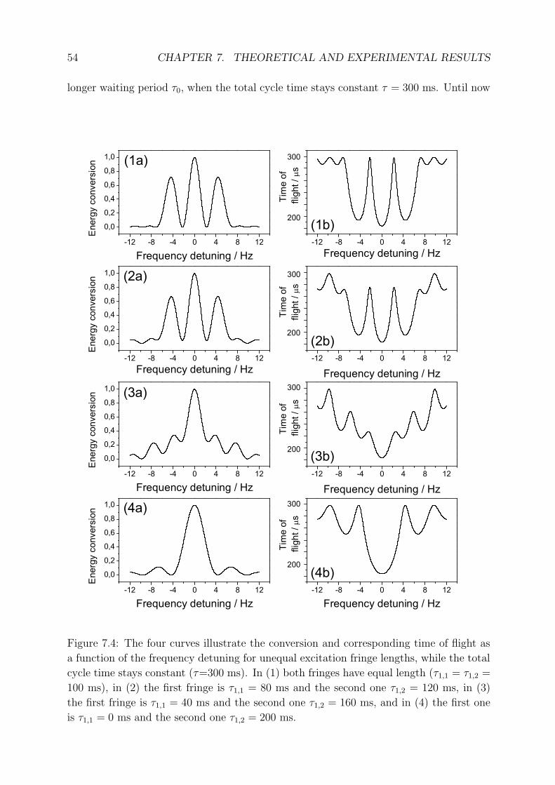
54 CHAPTER 7. THEORETICAL AND EXPERIMENTAL RESULTS
longer waiting period τ0, when the total cycle time stays constant τ = 300 ms. Until now
Figure 7.4: The four curves illustrate the conversion and corresponding time of flight as
a function of the frequency detuning for unequal excitation fringe lengths, while the total
cycle time stays constant (τ=300 ms). In (1) both fringes have equal length (τ1,1 = τ1,2 =
100 ms), in (2) the first fringe is τ1,1 = 80 ms and the second one τ1,2 = 120 ms, in (3)
the first fringe is τ1,1 = 40 ms and the second one τ1,2 = 160 ms, and in (4) the first one
is τ1,1 = 0 ms and the second one τ1,2 = 200 ms.

7.1. THEORETICAL INVESTIGATIONS 55
the considerations were restricted to symmetric excitation schemes with equal lengths τ1
of the two excitation fringes. But this restriction is experimentally not mandatory al-
though it simplifies the measurement procedure. In Fig. 7.4 the energy conversion and
the corresponding time of flight of four excitation schemes with two fringes are shown.
The total cycle time is kept constant to be τ = 300 ms and the waiting time is fixed to
τ0 = 100 ms. In (1) the symmetric excitation scheme is shown, where both excitation
periods have the same length of τ1,1 = τ1,2 = 100 ms. This was already discussed before.
In opposite to that, in (2) the first excitation period is τ1,1 = 80 ms and the other one
is τ1,2 = 120 ms, while in (3) the first excitation period is τ1,1 = 40 ms and the other
one is τ1,2 = 160 ms. The shape of the curve is independent whether the short excitation
period comes first or second. (4) illustrates the extreme case, where one fringe disappears
(τ1,1 = 0) and the second fringe becomes maximal (τ1,1 = 200 ms). This is identical to a
one-fringe excitation scheme with 200 ms excitation time.
In Fig. 7.5 the calculated FWHM for various lengths of the first excitation fringe is shown.
The total cycle time is 900 ms and the waiting time is kept constant at τ0 = 300 ms. The
smallest line-width occurs, when the first fringe is 300 ms, which implies that the second
fringe is also 300 ms. The symmetry of the curve with respect to a vertical axis through
the x-value of 300 ms shows, that the resulting profile is independent of the ordering of
the two fringes. Since the smallest line width leads to the most precise frequency de-
termination, the symmetric excitation scheme is the best and is thus the only one to be
considered in the following.
Figure 7.5: The total cycle time of the two-fringe excitation scheme is 900 ms and the
waiting time is fixed to τ0 = 300 ms. The theoretical FWHM versus the length of the
first excitation fringe is shown.

56 CHAPTER 7. THEORETICAL AND EXPERIMENTAL RESULTS
The three-fringe excitation scheme
Figure 7.6: The energy conversions of the three-fringe excitation schemes are shown in the
left column (a) and the corresponding time-of-flight curves are given in the right column
(b). For all graphs the total cycle time is τ = 300 ms. The excitation time of each fringe
is 100 ms (1), 66.7 ms (2), 40 ms (3), and 13.3 ms (4). The energy conversions of these
excitation schemes are shown in the left column (a) and the corresponding time-of-flight
curves are given in the right column (b).

7.1. THEORETICAL INVESTIGATIONS 57
For simplification the three-fringe excitation as well as the four-fringe excitation scheme
will only be discussed for fringes with equal length, i.e. all excitation periods have the
same length as well as all waiting periods have identical length.
In Fig. 7.6 the conversion graphs and the time-of-flight spectra for a scheme with three
excitation fringes are shown. The main difference in comparison to the two-fringe excita-
tion scheme is the existence of smaller side peaks between two main peaks. Similar to the
two-fringe excitation the shape of the curve can be explained by inner structure which is
formed by an envelope. In Fig. 7.6 (1) the length of each excitation period is τ1 = 100
ms, which is in total the overall cycle time of τ = 300 ms, i.e. identical to the one-fringe
scheme. Shorter excitation periods, as shown in (2), where one fringe is 66.7 ms, reduce
the width of the resonance in the same way as it was demonstrated for the two-fringe case.
The excitation periods in (3) and (4) are 40 ms and 13.3 ms, respectively. The FWHM
of the peaks decrease between (1) and (4) accordingly.
The considerations of the analogy to the optical slit experiment can be proceeded. The
intensity distribution after the three-slit configuration is shown in Fig. 7.3. There is an
easy rule for the correlation between the inner structure of the intensity distribution and
the number of slits. A system with n slits delivers an intensity distribution with n − 1
minima and n − 2 small peaks between two main peaks. The form of the envelope is
determined by the form of the slits. That means, that a rectangular slit results in an
intensity distribution that can be described by the sinc-function, which is the Fourier
transformation of a rectangular shaped profile.
The four-fringe excitation scheme
As well as in the three-fringe excitation scheme the four-fringe excitation is only done with
equal lengths of the excitation periods τ1 and equal lengths of the waiting periods τ0. In
the analogy to the optical system described in the previous sections the inner structure
(see Fig. 7.7) consists of main peaks interrupted by pairs of smaller side peaks. The en-
velope is determined as usual by the length of one individual excitation fringe. The peak
widths in the case of the energy conversion figures (a) and correspondingly the resonance
widths of the time-of-flight resonances (b) decrease analog to the two- and three-fringe
excitation schemes with decreasing length of the excitation fringes, i.e. with increasing
length of the waiting periods. A quantification of the calculations and a detailed compar-
ison with experimental results will be given in the next section. Here, only a summary of
the theoretical results is given.
The curves for the theoretically calculated FWHM of the TOF resonances for different
excitation times and schemes are shown in Fig. 7.10 (solid lines). The largest FWHM
is obtained for the cycle with the longest excitation times, which is identical with the
standard one-fringe excitation. The expected value is ∆ν = 4.0 Hz. The smallest FWHM
is obtained for the shortest excitation fringes, i.e. the longest waiting periods. In the
two-fringe scheme the shortest used excitation period is τ1 = 20 ms which was deter-
mined by the maximum possible quadrupolar radiofrequency amplitude to still obtain
one conversion, and thus the total excitation time is 40 ms. The value of the FWHM for
this scheme is ∆ν = 2.6 Hz, which corresponds to a reduction of 35% compared to the
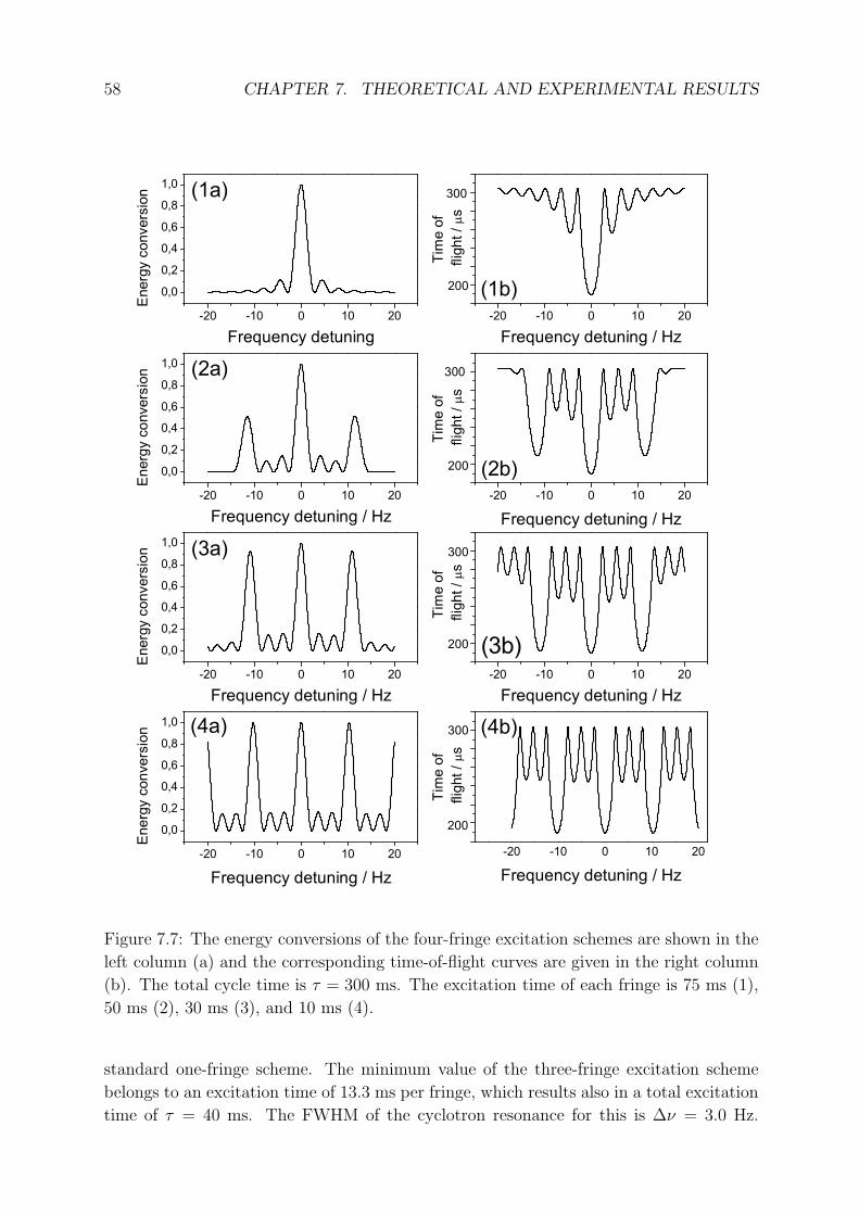
58 CHAPTER 7. THEORETICAL AND EXPERIMENTAL RESULTS
Figure 7.7: The energy conversions of the four-fringe excitation schemes are shown in the
left column (a) and the corresponding time-of-flight curves are given in the right column
(b). The total cycle time is τ = 300 ms. The excitation time of each fringe is 75 ms (1),
50 ms (2), 30 ms (3), and 10 ms (4).
standard one-fringe scheme. The minimum value of the three-fringe excitation scheme
belongs to an excitation time of 13.3 ms per fringe, which results also in a total excitation
time of τ = 40 ms. The FWHM of the cyclotron resonance for this is ∆ν = 3.0 Hz.

7.2. EXPERIMENTAL RESULTS 59
Thus, one obtains a reduction in the FWHM by about 25%. The smallest FWHM using
a four-fringe excitation is ∆ν = 3.3 Hz, which corresponds to a gain of about 20%, i.e.
a factor of two less than with the two-fringe scheme. These results of the investigations
of the FWHM show clearly that the two-fringe excitation scheme will allow for the most
precise determination of the cyclotron frequency.
7.2 Experimental results
To verify the theoretical calculations, i.e. to determine the line-width reduction and,
most important, to specify the gain in precision by using the Ramsey excitation method,
more than 300 time-of-flight resonance curves were taken with the Penning trap mass
spectrometer ISOLTRAP. The used ion species for all measurements was 39K+ from the
off-line surface ion source and each resonance consists of 3000 ions. To minimize ion-ion
interactions it was tried to store only one to three ions simultaneously. Altogether six se-
ries of measurements have been performed, each with several weeks of measurement time.
The most effort was done to determine the uncertainty in the frequency determination
for different excitation schemes. To this end, TOF resonances with two, three and four
excitation fringes were taken, with a fixed total cycle time in the precision trap of τ = 300
ms. To be able to compare the different excitation schemes the length of the fringes was
chosen properly. Figure 7.8 shows four TOF resonances where the sum of excitation times
τ1 was kept constant to 200 ms. The shape of the measured curves is evidently identical to
the calculated ones shown in Fig. 7.1 (1b), Fig. 7.2 (2b), Fig. 7.6 (2b), and Fig. 7.7 (2b).
A fit of the theoretically expected line shape (solid line) to the data points allows the
determination of the FWHM and the cyclotron frequency νc along with the uncertainty
δνc. To perform these fits the standard evaluation program of ISOLTRAP was extended
within this work in order to analyze the measured cyclotron resonances using the Ramsey
method.
The fit results concerning the FWHM are presented in Fig. 7.9 and Fig. 7.10. In Fig. 7.9
the error bars are hardly visible, since they have almost the same size as the symbols
of the data points. Fig. 7.9 shows results obtained with a two-fringe excitation scheme
of different overall cycle times (τ =300 ms, 600 ms, 900 ms). The FWHM is given as
a function of the sum of the excitation periods. Similar results are shown in Fig. 7.10
but for a different number of Ramsey excitation fringes. The solids line under the data
points are the calculated FWHM. The experimental values are in average 0.1 Hz larger
than the theoretical ones. This effect, called line broadening, results from the electric
and magnetic field imperfections and ion-ion interactions as explained in Chap. 2.2. A
significant reduction of the FWHM at shorter excitation fringes is visible.
In Tab. 7.1 the experimental results are summarized. “Number” declares the number of
fringes, “time” is the duration of the total cycle. The maximal FWHM is the FWHM
of the standard one-fringe resonance curve. The minimal FWHM is measured using the
shortest possible excitation time which is determined by the maximal possible amplitude
of the quadrupolar excitation field required to obtain one full conversion from pure mag-
netron to pure cyclotron motion. For the 300 ms cycle this minimal sum excitation time

60 CHAPTER 7. THEORETICAL AND EXPERIMENTAL RESULTS
Figure 7.8: In all four figures the measured mean time of flights and their fitting curves
(solid lines) are shown. In (a) the resonance of the so far used standard one-fringe excita-
tion scheme is shown. (b) illustrates the TOF of a two-fringe excitation scheme with two
times 100 ms excitation and 100 ms waiting time. In (c) the excitation is done by three
fringes, each 66.67 ms, interrupted by two waiting periods of 50 ms. (d) shows the TOF
of four 50 ms excitation fringes and three waiting periods of 33.33 ms.
is always 40 ms. The shortest sum excitation time of the 600 ms cycle is 60 ms and in
the case of the 900 ms cycle it is 90 ms. The last column of Tab. 7.1 gives the maximum
gain in line-width reduction using the different Ramsey excitation schemes. A remarkable
reduction of close to half of the normal line-width is observed, similar to the results in the
original work of Ramsey [Rams1990] with a total different application of this technique.
The reduction in line-width is of especially importance in context of the achievable re-
solving power R = m∆m
= ν∆ν
. As expected, the best possible reduction is obtained by a
two-fringe excitation scheme. The relative gain in reduction is independent of the length
of the total excitation cycle (see Tab. 7.1).
In Fig. 7.11 the evaluated uncertainty δνc of the cyclotron frequency determination
for a different number of Ramsey fringes versus the waiting time τ0 is plotted (circles).
To be conservative the error of this uncertainty was adopted to be 10%. Each data
point represents the mean value of three to ten individual measurements. In general the
uncertainty δνc decreases, when the waiting time increases. This was expected due to
the decreasing FWHM at longer waiting times. If the cyclotron frequency uncertainty

7.2. EXPERIMENTAL RESULTS 61
Figure 7.9: The full-width-half-maximum values (FWHM) of the time-of-flight cyclotron
resonances as a function of the sum excitation time for the two-fringe excitation scheme
is given. The total cycle time τ is 300 ms (squares), 600 ms (triangles), and 900 ms
(circles). The solid lines below the lines of data points are the theoretically calculated
curves of the FWHM. Since the determination of the FWHM has to be done manually
from the fit curves the error bars are conservatively estimated to be ±0.05 Hz. Due to
field inhomogeneities and ion-ion interactions the data points are shifted a little bit to
higher FWHM values compared to theory.
would only depend on the FWHM, one would expect a similar behavior as observable in
Fig. 7.10,i.e. a smooth trend to smaller uncertainties with increasing waiting times. How-
ever, as mentioned before, there are strong hints that there is also an effect of the overall
line-shape, especially of the steepness of the curve, on the uncertainty of the frequency
νc. To verify this assumption, to all plots the inverse average steepness of the theoretical
resonance curves (triangles) for the respective waiting times are added. A further detailed
investigation of the importance of each single frequency point on the cyclotron frequency
uncertainty δνc will be presented in the diploma thesis of Michael Dworschak [Dwor2006].
Also the advantage of taking non-equidistant step sizes with different weights, i.e. differ-
ent numbers of ions per frequency step, which will be of special importance in respect to

62 CHAPTER 7. THEORETICAL AND EXPERIMENTAL RESULTS
Figure 7.10: The full-width-half-maximum (FWHM) values of the time-of-flight cyclotron
resonances as a function of the sum excitation times is given for a different number of
excitation fringes. The solid lines below the data points are the theoretically calculated
curves of the FWHM. The data points with 300 ms excitation time are shifted 5 ms
against each other in the plot for better visibility.
the Ramsey excitation method, will be discussed there.
In Fig. 7.11 the uncertainty of the cyclotron frequency δνc as a function of the waiting τ0
is shown for different excitation schemes. In Fig. 7.11(a) the excitation scheme consists
of two fringes, whereas the total excitation cycle is fixed to 300 ms. The uncertainty is
obviously decreasing with shorter excitation fringes, i.e longer waiting times τ0. Notice-
able local fluctuations in this trend can be explained by the curve of the inverse steepness
of the resonance curve. A high value in this curve means that the average steepness of
the curve is small as it is the case when sidebands are not that much enhanced. One can
say, the steeper the resonance curve, i.e. the stronger the sidebands are pronounced, the
better the center frequency νc can be determined. Thus local minima or maxima in the
curve of the uncertainties are also visible in the curve of the steepness. This behavior is
also observable in the other five figures of Fig. 7.11.
Finally, most important is the fact, that the statistical uncertainty in the cyclotron fre-
quency determination for an overall cycle time of τ = 300 ms can be reduced by more

7.2. EXPERIMENTAL RESULTS 63
Table 7.1: In this tabular the maximum and minimum experimental FWHM of the differ-
ent excitation schemes for different cycle times are given. In addition the reduction gain
calculated.
number of fringes cycle time max. FWHM min. FWHM reduction gain
Hz Hz %
4 300 4.1 3.3 20.5 (2.7)
3 300 4.1 3.0 26.5 (2.2)
2 300 4.1 2.6 37.3 (2.0)
2 600 2.1 1.3 38.1 (4.0)
2 900 1.4 0.9 65.7 (5.9)
than a factor of three (from δνc = 25 mHz down to δνc = 7 mHz) just by changing the
excitation scheme to the here proposed two-fringe Ramsey method. One should keep in
mind that the total number of ions per resonance curve was kept constant to 3000 ions.
The result is also summarized in Tab. 7.2. In Fig. 7.11(b) and Fig. 7.11(c) the uncertain-
ties of the three- and four-fringe excitation for a 300 ms cycle are plotted. Figure 7.11
(d) and (e) show the uncertainty of two larger two-fringe excitation schemes. The total
excitation times are 600 ms (d) and 900 ms (e). In Fig. 7.11 (f) the uncertainty δνc of the
fit is illustrated versus the excitation time of one fringe for a non-symmetric excitation
scheme. The waiting time is always 100 ms and the total excitation cycle is 300 ms. The
length of the second fringe plus the length of the fringe given on x-axis is constant 200 ms.
The uncertainty becomes minimal when both fringes are of equal length consistent with
the theoretical predictions shown in Fig. 7.5. The maximal and the minimal uncertainty
for all investigated excitation schemes are listed in Tab. 7.2. As for the investigation of the
FWHM the scheme where the biggest reduction in the cyclotron frequency uncertainty can
be gained is the two-fringe Ramsey scheme. Comparing the two fringe excitation scheme
with 300 ms, 600 ms, and 900 ms total cycle time the tendency is similar to the results
obtained for the FWHM of the resonances. The differences in the gain factor between the
different two-fringe schemes must be assigned to the steepness effects discussed before. To
conclude, the investigations showed, that an optimized Ramsey excitation scheme with
two excitation fringes of short duration interrupted by a maximal waiting period results
in an improvement of the statistical uncertainty in the cyclotron frequency determination
by more than a factor of three, keeping the number of ions constant.

64 CHAPTER 7. THEORETICAL AND EXPERIMENTAL RESULTS
Figure 7.11: In (a) to (e) figures the uncertainty in the determination of the cyclotron
frequency is plotted versus the waiting time (circles). In addition, the reciprocal derivation
versus the waiting time (triangles) is shown. In (a) the two-fringe excitation scheme with
a total cycle time of 300 ms is used. (b) and (c) show the three-fringe respectively the
four-fringe excitation results with a total cycle time of 300 ms. Figure (d) and (e) show
again the two fringe excitation results, but with a total cycle time of 600 ms respectively
900 ms. In (f) δνc is plotted against the excitation time of one fringe to show the effect
of a non-symmetric excitation scheme.
Table 7.2: The maximal and the minimal uncertainties of different excitation schemes
and excitation times are presented. The calculated improvement factor is given in the
last column.
number of fringes cycle time max. uncertainty min. uncertainty Improvement
Hz Hz factor
4 300 0.027 0.017 1.6 (0.2)
3 300 0.028 0.014 2.0 (0.2)
2 300 0.025 0.007 3.6 (0.4)
2 600 0.017 0.006 2.8 (0.3)
2 900 0.010 0.004 2.5 (0.3)
2 unequal 0.037 0.023 1.6 (0.2)

Chapter 8
Summary and Outlook
During this diploma thesis an experimental improvement was developed and implemented
in the setup of ISOLTRAP: The common one-fringe quadrupolar excitation scheme for
the manipulation of the motion of the stored ions was replaced by an excitation using sep-
arated oscillatory quadrupole radiofrequency fields. This is the so called Ramsey method.
The idea to use the Ramsey method for the measurement of the time-of-flight cyclotron
resonance in Penning trap mass spectrometry was already proposed more than 10 years
ago at ISOLTRAP [Boll1992] but due to a missing full theoretical description of the result-
ing line-shapes not yet implemented and further investigated. In this context the mathe-
matical description of the ion motion in presence of the separated oscillatory quadrupole
fields has been carried out and the resulting time-of-flight resonance curves derived. The
data fitting routines using these equations have been implemented in the evaluation pro-
gram of ISOLTRAP. The calculated line profiles show that the most benefiting excitation
scheme in view of the resonance line-width is the one with two separated excitation fringes
of equal length being as short as possible. The maximum demonstrated reduction of the
line-width using the proposed two-fringe Ramsey scheme was 40%, so almost half of the
normal line-width.
In the experimental part of this work the Ramsey method was implemented at ISOLTRAP
and a large amount of measurements performed comparing the two-, three-, and four fringe
excitation scheme. In agreement to the theoretical predictions is has been shown that the
best excitation scheme is the one with two short excitation periods interrupted by a certain
waiting time. Within the expected experimental imperfections, here especially inhomo-
geneities of the magnetic field, the theoretical results concerning the line-width have been
confirmed. The analytical solution of the system: ion, Penning trap configuration, and
external separate oscillatory fields, has been used to evaluate the measured time-of-flight
cyclotron resonances by least-squares fits. The most important result obtained within
this thesis is the fact, that the uncertainty in the frequency determination and thus the
uncertainty of the mass of the nuclide of interest can be improved by a factor of three
using the best suited Ramsey excitation scheme. This investigation is in coherence with
a series of exciting developments in high-precision Penning trap mass spectrometry, in-
cluding new cooling, excitation, and detection schemes, in order to improve the accuracy
of mass measurements of stable and short-lived nuclides.
65

66 CHAPTER 8. SUMMARY AND OUTLOOK
In the course of this diploma thesis, several suggestions for further developments and
investigations have turned up:
1. The theoretical calculations of the time-of-flight resonance line-shapes obtained with
the Ramsey method should be extended to include also damping effects caused by
rest-gas collisions. This would allow to use longer quadrupolar excitation times re-
sulting in higher resolving powers and still being able to fit the measured resonances.
2. Measurements with real contaminants, i.e. more than one ion specie in the precision
Penning trap, have to be made. This would allow to study the effect of contamina-
tions on the TOF resonance line-shape using the Ramsey excitation method.
3. Mass measurements of radionuclides using the investigated Ramsey excitation
method have to be performed in order to demonstrate the precision gain also in
on-line mass measurements. Due to a limited number of ISOLTRAP data taking
periods per year getting radionuclides from ISOLDE (in total 22 shifts of 8 hours
during this year) this has not done be so far.
4. Until now equidistant frequency steps are used for the scan of the quadrupolar
excitation frequency around νc. As it became obvious during this thesis, a non-
equidistant distribution of the frequency steps having different statistical weights,
i.e. collecting different numbers of ions per step, might be of advantage although
its experimental implementation is difficult. This project has already started within
the diploma thesis of Michael Dworschak [Dwor2006].

Bibliography
[Ande1962] P.W. Anderson, Phys. Rev. Lett. 9 (1962) 309.
[Ande1964] P.W. Anderson, Y.B. Kim, Rev. Mod. Phys. 39 (1964) 39.
[Audi2003] G. Audi, A.H. Wapstra and C. Thibault, Nucl. Phys. A 729 (2003) 337.
[Berg2002] I. Bergstrom, C. Carlberg, T. Fritioff, G. Douysset, J. Schonfelder, R. Schuch,
Nucl. Instr. and Meth. A 487 (2002) 618.
[Blau2002] K. Blaum, G. Bollen, F. Herfurth, A. Kellerbauer, H.-J. Kluge, M. Kuckein,
E. Sauvan, C. Scheidenberger, L. Schweikhard, Eur. Phys. J. A 15 (2002) 245.
[Blau2003] K. Blaum, D. Beck, G. Bollen, F. Herfurth, A. Kellerbauer, H.-J. Kluge, R.B.
Moore, E. Sauvan, C. Scheidenberger, S. Schwarz, L. Schweikhard, Nucl. Instr. and
Meth. B 204 (2003) 478.
[Blau2003b] K. Blaum, G. Audi, D. Beck, G. Bollen, F. Herfurth, A. Kellerbauer, H.-J.
Kluge, E. Sauvan, S. Schwarz, Phys. Rev. Lett. 91 (2003) 260801.
[Blau2004] K. Blaum, G. Audi, D. Beck, G. Bollen, P. Delahaye, C. Guenaut, F. Herfurth,
A. Kellerbauer, H.-J. Kluge, D. Lunney, D. Rodrıguez, S. Schwarz, L. Schweikhard,
C. Weber, C. Yazidjian, Nucl. Phys. A 746 (2004) 305c.
[Blau2004] K. Blaum, D. Beck, G. Bollen, P. Delahaye, C. Guenaut, F. Herfurth, A.
Kellerbauer, H.-J. Kluge, D. Lunney, S. Schwarz, L. Schweikhard, C. Yazidjian, Eu-
rophys. Lett. 67 (2004) 586.
[Blau2005] K. Blaum, G. Audi, D. Beck, G. Bollen, M. Brodeur, P. Delahaye, S. George,
C. Guenaut, F. Herfurth, A. Herlert, A. Kellerbauer, H.-J. Kluge, D. Lunney, M.
Mukherjee, D. Rodrıguez, S. Schwarz, L. Schweikhard, and C. Yazidjian J. Phys. G,
in print (2005).
[Boll1990] G. Bollen, R.B. Moore, G. Savard, H. Stolzenberg, J. Appl. Phys. 68 (1990)
4355.
[Boll1992] G. Bollen, H.-J. Kluge, M. Konig, T. Otto, G. Savard, H. Stolzenberg, R.B.
Moore, G. Rouleau, G. Audi, ISOLDE Collaboration, Phys. Rev. C 46 (1992) R2140.
67

68 BIBLIOGRAPHY
[Boll1996] G. Bollen, S. Becker, H.-J. Kluge, M. Konig, R.B. Moore, T. Otto, H.
Raimbault-Hartmann, G. Savard, L. Schweikhard, H. Stolzenberg, ISOLDE Collab-
oration, Nucl. Instr. and Meth. A 368 (1996) 675.
[Boll2001] G. Bollen, Nucl. Phys. A 693 (2001) 3.
[Boll2004] G. Bollen, Lect. Notes Phys. 651 (2004) 169.
[Brad1999] M.P. Bradley, J.V. Porto, S. Rainville, J.K. Thompson, D.E. Pritchard, Phys.
Rev. Lett. 83 (1999) 4510.
[Brow1986] L.S. Brown, G. Gabrielse, Rev. Mod. Phys. 58 (1986) 233.
[Yazi2006] C. Yazidjian, in preparation, PHD thesis, University of Caen, France (2006)
[Dehm1990] H. Dehmelt, Rev. Mod. Phys. 62 (1990) 525.
[Dwor2006] M. Dworschak, in preparation, Diplomarbeit, Universitat Wurzburg (2006).
[Dyck1992] R.S. Van Dyck, Jr., D.L. Farnham, P.B. Schwinberg, J. Mod. Opt. 39 (1992)
243.
[Graf1980] G. Graff, H. Kalinowsky, J. Traut, Z. Phys. A 297 (1980) 35.
[Hard2005a] J.C. Hardy, I.S. Towner, Phys. Rev. C 71 (2005) 055501.
[Hard2005b] J.C. Hardy, I.S. Towner, Phys. Rev. Lett. 94 (2005) 092502
[Herf2001a] F. Herfurth, J. Dilling, A. Kellerbauer, G. Bollen, S. Henry, H.-J. Kluge,
E. Lamour, D. Lunney, R.B. Moore, C. Scheidenberger, S. Schwarz, G. Sikler, J.
Szerypo, Nucl. Instr. and Meth. A 469 (2001) 254.
[Herf2001b] F. Herfurth, J. Dilling, A. Kellerbauer, G. Audi, D. Beck, G. Bollen, S. Henry,
H.-J. Kluge, D. Lunney, R. B. Moore, C. Scheidenberger, S. Schwarz, G. Sikler, J.
Szerypo, ISOLDE Collaboration, in: Proc. “Atomic Physics at Accelerators: Mass
Spectrometry (APAC 2000)”, Cargese, France, 2000 (eds. D. Lunney, G. Audi, H.-J.
Kluge), Hyp. Int. 132 (2001) 309.
[Herf2003] F. Herfurth, F. Ames, G. Audi, D. Beck, K. Blaum, G. Bollen, A. Kellerbauer,
H.-J. Kluge, M. Kuckein, D. Lunney, R.B. Moore, M. Oinonen, D. Rodrıguez, E.
Sauvan, C. Scheidenberger, S. Schwarz, G. Sikler, C. Weber, ISOLDE Collaboration,
J. Phys. B 36 (2003) 931.
[Kell2001] A. Kellerbauer, T. Kim, R.B. Moore, P. Varfalvy, Nucl. Instr. and Meth. A
469 (2001) 276.
[Kell2003] A. Kellerbauer, K. Blaum, G. Bollen, F. Herfurth, H.-J. Kluge, M. Kuckein,
E. Sauvan, C. Scheidenberger, L. Schweikhard, Eur. Phys. J. D 22 (2003) 53.

BIBLIOGRAPHY 69
[Kell2004] A. Kellerbauer, G. Audi, D. Beck, K. Blaum, G. Bollen, P. Delahaye, F. Her-
furth, H.-J. Kluge, V. Kolhinen, M. Mukherjee, D. Rodrıguez, and S. Schwarz Nucl.
Phys. A 746 (2004) 635c.
[Kell2004b] A. Kellerbauer, G. Audi, D. Beck, K. Blaum, G. Bollen, B.A. Brown, P. Dela-
haye, C. Guenaut, F. Herfurth, H.-J. Kluge, D. Lunney, S. Schwarz, L. Schweikhard,
C. Yazidjian, Phys. Rev. Lett. 93 (2004) 072502.
[Koni1991] M. Konig, Massenspektrometrische Aufloesung von Isomer und Grundzustand
in einer Penningfalle und Untersuchungen zur Coulombwechselwirkung gespeicherter
Ionen, Diplomarbeit, Johannes Gutenberg-Universitat Mainz (1991).
[Koni1995a] M. Konig, G. Bollen, H.-J. Kluge, T. Otto, J. Szerypo, Int. J. Mass Spec.
Ion Process. 142 (1995) 95.
[Koni1995b] M. Konig, Prazisionsmassenbestimmung instabiler Casium- und Bariumio-
nen in einer Penningfalle und Untersuchung der Ionenbewegung bei azimuthaler
Quadrupolanregung, Dissertation, Johannes Gutenberg-Universitat Mainz (1995).
[Kost2003] U. Koster, V.N. Fedoseyev, V.I. Mishin, Spectrochim. Acta B 58 (2003) 1047.
[Kret1991] M. Kretzschmar, Eur. J. Phys. 12 (1991) 240.
[Kret1992] M. Kretzschmar, Physica Scripta 46 (1992) 544.
[Kret1999] M. Kretzschmar, Conf. Proc. ”Trapped Charged Particles and Fundamental
Physics”, Asilomar(California), 1998, Eds.: D.H.E.Dubin, D. Schneider, AIP Con-
ference Proceedings 457 (1999) 242.
[Kret2005] M. Kretzschmar, private communication (2005).
[Kugl2000] E. Kugler, Hyperfine Interactions 129 (2000) 23.
[Lunn2003] D. Lunney, J.M. Pearson, C Thibault, Rev. Mod. Phys. 75 (2003) 1021.
[Majo2005] F.G. Major, V.N. Gheorghe, G. Werth, Charged Particle Traps, Physics and
Techniques of Charged Particle Field Confinement (Springer Series on Atomic, Op-
tical, and Plasma Physics, Vol. 37). Springer, Berlin (2005).
[Mukh2004] M. Mukherjee, A. Kellerbauer, D. Beck, K. Blaum, G. Bollen, F. Carrel, P.
Delahaye, J. Dilling, S. George, C. Guenaut, F. Herfurth, A. Herlert, H.-J. Kluge,
U. Koster, D. Lunney, S. Schwarz, L. Schweikhard, C. Yazidjian, Phys. Rev. Lett. 93
(2004) 150801.
[Qui1998] T.J. Quinn, I.M. Mills, in: The International System of Units (SI), The SI
Brochure, 7th Edition, Bureau International des Poids et Mesures, Sevres, France,
1998, p. 152.
[Rabi1938] I.I. Rabi, J.R. Zacharias, S. Millman, and P. Kusch, Phys. Rev. 53 (1938) 318.

70 BIBLIOGRAPHY
[Rabi1939] I.I. Rabi, J.R. Zacharias, S. Millman, and P. Kusch, Phys. Rev. 55 (1939) 526.
[Raim1997] H. Raimbault-Hartmann, D. Beck, G. Bollen, M. Konig, H.-J. Kluge, E.
Schark, J. Stein, S. Schwarz, J. Szerypo, Nucl. Instr. and Meth. B 126 (1997) 378.
[Rams1990] N. Ramsey, Rev. Mod. Phys. 62 (1990) 541.
[Rodr2004] D. Rodrıguez, V.S. Kolhinen, G. Audi, J. Aysto, D. Beck, K. Blaum, G.
Bollen, F. Herfurth, A. Jokinen, A. Kellerbauer, H.-J. Kluge, M. Oinonen, H. Schatz,
E. Sauvan, S. Schwarz, Phys. Rev. Lett. 93 (2004) 161104.
[Roos2004] J. Van Roosbroeck, C. Guenaut, G. Audi, D. Beck, K. Blaum, G. Bollen, J.
Cederkall, P. Delahaye, H. De Witte, D. Fedorov, V.N. Fedoseyev, S. Franchoo, H.
Fynbo, M. Gorska, F. Herfurth, K. Heyde, M. Huyse, A. Kellerbauer, H.-J. Kluge,
U. Koster, K. Kruglov, D. Lunney, A. De Maesschalck, V.I. Mishin, W.F. Muller, S.
Nagy, S. Schwarz, L. Schweikhard, N.A. Smirnova, K. Van de Vel, P. Van Duppen,
A. Van Dyck, W.B. Walters, L. Weissmann, C. Yazidjian, Phys. Rev. Lett. 92 (2004)
112501.
[Sava1991] G. Savard, St. Becker, G. Bollen, H.-J. Kluge, R.B. Moore, Th. Otto, L.
Schweikhard, H. Stolzenberg, U. Wiess, Phys. Lett. A 158 (1991) 247.
[Schw2001] S. Schwarz, F. Ames, G. Audi, D. Beck, G. Bollen, C. De Coster, J. Dilling,
O. Engels, R. Fossion, J.-E. Garcia Ramos, S. Henry, F. Herfurth, K. Heyde, A.
Kellerbauer, H.-J. Kluge, A. Kohl, E. Lamour, D. Lunney, I. Martel, R.B. Moore,
M. Oinonen, H. Raimbault-Hartmann, C. Scheidenberger, G. Sikler, J. Szerypo, C.
Weber, ISOLDE collaboration, Nucl. Phys. A 693 (2001) 533.
[West1984] B.J. West, K. Lindenberg, Phys. Rev. 102A (1984) 189.

Acknowledgements
Here I want to use the possibility to thank some people:
D. Frekers for the confidence, which opened me the possibility to perform an external
thesis at the European Organization for Nuclear Research (CERN), for the support of
my CERN applications. The stays at CERN belong to the most impressing experiences
of my studies.
K. Blaum for his indescribable care and support in the last two years at ISOLTRAP and
in Mainz. Without him and his advices this work would not be possible. Thank you very
much.
M. Kretzschmar for support and scientific advice, for the many fruitful discussions.
S. Schwarz for answering the many questions related to the evaluation program and its
extension.
P. Delahaye, M. Dworschak, Celine Guenaut, F. Herfurth, A.J. Herlert, A. Kellerbauer,
H.-J. Kluge, D. Lunney, L. Schweikhard, and C. Yazidjian for the fruitful work at
ISOLTRAP.
S. Djekic, M. Dworschak, S. Kreim, R. Ferrer, J. Verdu and C. Weber for the great
working group at the university of Mainz.
But there are outside the physics people supporting me strongly:
My parents, Doris and Armin, and my brother Kilian. Their commitment and support
allowed my studies.
And Britta for her everlasting support.
71


![Penning Traps Neutrino Mass - Indico [Home]](https://img.pdfslide.net/doc/110x75/6176559f30056d79473180a3/penning-traps-neutrino-mass-indico-home.jpg)


