Embed Size (px)
Citation preview

Applied π – A Brief Tutorial
Peter Sewell
Computer Laboratory, University of [email protected]
July 28, 2000

2
Abstract
This note provides a brief introduction to π-calculi and their application to concurrentand distributed programming. Chapter 1 introduces a simple π-calculus and discussesthe choice of primitives, operational semantics (in terms of reductions and of indexedearly labelled transitions), operational equivalences, Pict-style programming and typing.Chapter 2 goes on to discuss the application of these ideas to distributed systems, lookinginformally at the design of distributed π-calculi with grouping and interaction primitives.Chapter 3 returns to typing, giving precise definitions for a simple type system andsoundness results for the labelled transition semantics. Finally, Chapters 4 and 5 providea model development of the metatheory, giving first an outline and then detailed proofsof the results stated earlier. The note can be read in the partial order 1.(2 + 3 + 4.5).
Contents
1 Pi Calculi 51.1 An Introduction to π . . . . . . . . . . . . . . . . . . . . . . . . . . . . . . 51.2 Modelling vs Programming: choices of primitives . . . . . . . . . . . . . . 71.3 Styles of Operational Semantics . . . . . . . . . . . . . . . . . . . . . . . . 91.4 Language Implementation: the Pict experiment . . . . . . . . . . . . . . 111.5 Operational Congruences . . . . . . . . . . . . . . . . . . . . . . . . . . . 121.6 Typing . . . . . . . . . . . . . . . . . . . . . . . . . . . . . . . . . . . . . . 141.7 Further Reading . . . . . . . . . . . . . . . . . . . . . . . . . . . . . . . . 15
2 Distributed π calculi 17
3 Simple Types 233.1 Polyadicity and Tuples . . . . . . . . . . . . . . . . . . . . . . . . . . . . . 233.2 Typing . . . . . . . . . . . . . . . . . . . . . . . . . . . . . . . . . . . . . . 253.3 Typing and Labelled Transitions . . . . . . . . . . . . . . . . . . . . . . . 26
4 Metatheory: Overview 294.1 Basic Properties of the LTS . . . . . . . . . . . . . . . . . . . . . . . . . . 294.2 Coincidence of the Two Semantics . . . . . . . . . . . . . . . . . . . . . . 334.3 Strong Bisimulation and Congruence . . . . . . . . . . . . . . . . . . . . . 344.4 Type Soundness and Subject Reduction . . . . . . . . . . . . . . . . . . . 35
5 Metatheory: Detailed Proofs 395.1 Basic Properties of the LTS . . . . . . . . . . . . . . . . . . . . . . . . . . 395.2 Coincidence of the Two Semantics . . . . . . . . . . . . . . . . . . . . . . 485.3 Strong Bisimulation and Congruence . . . . . . . . . . . . . . . . . . . . . 535.4 Type Soundness and Subject Reduction . . . . . . . . . . . . . . . . . . . 58
References 63
3
4 CONTENTS
Acknowledgements
These notes are partly based on lectures given at the Instructional Meeting on RecentAdvances in Semantics and Types for Concurrency: Theory and Practice held in July1998, supported by the MATHFIT initiative of the EPSRC and LMS, organised byRajagopal Nagarajan, Bent Thomsen and Lone Leth Thomsen. They also draw on achapter written for a forthcoming volume edited by Howard Bowman and John Derrick.I would like to thank these organisers and editors. Some of the technical developmentis based on joint work with Luca Cattani and Jan Vitek. I acknowledge support fromEPSRC grants GR/K 38403, GR/L 62290, and a Royal Society University ResearchFellowship.

Chapter 1
Pi Calculi
Concurrency and communication are fundamental aspects of distributed systems;a great deal of work in process calculi and other areas has developed techniques forprogramming, specification and reasoning about them. Another basic distributed phe-nomenon is name generation – many computational entities are dynamically created withfresh names; these names can often be communicated within or between machines. Theπ-calculus of Milner, Parrow and Walker [MPW92] generalised earlier process calculi byallowing fresh channel names to be dynamically created and communicated. This givesrise to great expressive power, allowing a very simple π-calculus to be used as the basisfor a concurrent programming language. It also involved the development of semantictechniques which can be directly applied to distributed systems. This chapter introducessome of the theory of π-calculi and their applications to concurrent programming. Itprovides only a brief and somewhat idiosyncratic introduction – for more detailed textsand pointers into the literature one should refer to Section 1.7.
We begin in Section 1.1 with a core π-calculus, giving some examples and definingthe operational semantics in a reduction-semantics style. In Section 1.2 we review themain design choices that give rise to the wide variety of π-calculi in use. Many aredriven by a particular theoretical result or application, particularly by whether the focusis on modelling or programming. In Section 1.3 we return to the operational semantics,defining a labelled transition semantics and relating it to the earlier reduction semantics.In Section 1.4 we consider the (concurrent, but not distributed) Pict programminglanguage, closely based on a π-calculus. In Section 1.5 we return again to semantics,defining operational congruences. A very brief introduction to typing for π-calculi isgiven in Section 1.6.
1.1 An Introduction to π
The π-calculus is a calculus (an idealised modelling/programming language) in whichcommunication between parallel processes is fundamental. Communication is on namedchannels: a process that offers an output of value v on the channel named c, writtencv , may synchronise with a parallel process that is attempting to read from c, writtencw .P . It differs from earlier process calculi in that new channel names can be createddynamically, passed as values along other channels, and then used themselves for com-munication. This gives rise to great expressive power – many computational formalisms,e.g. λ-calculi, can be smoothly translated into π-calculus.
Many different π-calculi have been introduced. Some of the differences are essentially
5

6 CHAPTER 1. PI CALCULI
minor choices of notation and style; some are important choices that are driven by theapplication or theory desired. In this section we introduce a core π-calculus which stillexhibits the essential phenomenon of new channel creation.
Syntax We take an infinite set N of names of channels, ranged over by a, b etc. Theprocess terms are then those defined by the grammar
P,Q ::= 0 nilP |Q parallel composition of P and Qcv output v on channel ccw .P input from channel cnew c in P new channel name creation
In cw .P the ‘formal parameter’ w binds in P ; in new c in P the c binds in P , with scopeas far to the right as possible (so new c in P |Q should be read as new c in (P |Q)). Wewill work up to alpha renaming of bound names, so whenever we write a term we actuallymean its alpha equivalence class. We write fn(P ) for the set of free names of P , definedby fn(0) = ∅, fn(P |Q) = fn(P ) ∪ fn(Q), fn(cv) = {c, v}, fn(cw .P ) = {c} ∪ (fn(P ) − w),fn(new c in P ) = fn(P )− c. We write {a/x}P for the process term obtained from P byreplacing all free occurrences of x by a, renaming as necessary to avoid capture.
Semantics – Examples The simplest form of semantics for this calculus consists of areduction relation – a binary relation between process terms, written P−→Q, indicatingthat P can perform a single step of computation to become Q. The definition of −→ willbe given later; here are some examples.
The calculus allows communication between an output and an input (on the samechannel) in parallel. Here the value a is being sent along the channel x:
xa | xu.yu −→ {a/u}(yu) = ya
There can be many outputs on the same channel competing for the same input – onlyone will succeed, introducing nondeterminism:
xb | ya
xa | xb | xu.yu
xa | yb
Similarly, there can be many inputs on the same channel competing for an output:
ya | xu.zu
xa | xu.yu | xu.zu
xu.yu | za
A restricted name is different from all other names outside its scope – below the x boundby the new x in is different from the x outside. Note that (using alpha equivalence)the term on the left below is the same term as xa |new x ′ in (x ′b | x ′u.yu).
xa |new x in (xb | xu.yu) −→ xa |new x in yb
A name received on a channel can then be used itself as a channel name for output orinput – here y is received on x and then used to output c:
xy | xu.uc −→ yc

1.2. MODELLING VS PROGRAMMING: CHOICES OF PRIMITIVES 7
Finally (and most subtlely), a restricted name can be sent outside its original scope. Herey is sent on channel x outside the scope of the new y in binder, which must thereforebe moved (with care, to avoid capture of other instances of y). This is known as scopeextrusion:
(new y in xy | yv .P ) | xu.uc −→ new y in yv .P | yc−→ new y in {c/v}P
The combination of sending channel names and scope extrusion is the essential differencebetween the π-calculus and earlier process calculi such as ACP, CCS and CSP.
Semantics – Definition of Reduction The reduction relation can be defined rathersimply, in two stages. First we define a structural congruence, written ≡. This is anequivalence relation over process terms that allows the two parts of a potential commu-nication to be brought syntactically adjacent. It is the smallest equivalence relation thatis a congruence and satisfies the axioms:
P | 0 ≡ PP |Q ≡ Q |P
P |(Q |R) ≡ (P |Q) |Rnew x in new y in P ≡ new y in new x in P
P |new x in Q ≡ new x in (P |Q) x 6∈ fn(P )
The reduction relation −→ is then the smallest binary relation over process terms satis-fying the following.
Com cv | cw .P−→{v/w}P
ParP−→P ′
P |Q−→P ′ |Q
ResP−→P ′
new x in P−→new x in P ′
StructP ≡ P ′−→P ′′ ≡ P ′′′
P−→P ′′′
Note that reduction under input prefixes is not allowed – there is no rule
P−→P ′
cw .P−→cw .P ′
It is a useful exercise to check that the example reductions can actually be derived.
1.2 Modelling vs Programming: choices of primitives
A good deal of early work on process calculi was focussed around modelling protocols (andother systems) and reasoning about those models; this fed into work e.g. on Lotos andits descendents. Some recent developments from the π-calculus, in contrast, have usedit as the basis for a programming language: a significant shift of emphasis which affectsthe design of the calculi used. The programming language view is discussed further inSection 1.4 below; this subsection reviews some of the main calculus-design choices. Theyare here described rather informally – in some cases precise results have been proved,showing that a particular calculus is encodable in another, but great care must be taken

8 CHAPTER 1. PI CALCULI
in interpreting such results. There are many possible senses of ‘encoding’; the results donot automatically transfer from the precise calculi they have been proved for to minorvariants thereof. In general, we have only the beginnings of a theory of expressivenessfor π-based calculi (but see the recent EXPRESS meetings such as [PC98]).
Choice Many process calculi have explicit choice or summation operators for nonde-terminism, allowing for example P + Q which can behave either as P or as Q (this isimprecise – in fact several different operators are possible). Explicit choice is useful formodelling and reasoning about systems, especially for writing loose specifications and fordeveloping complete axiomatisations of operational congruences, but seems to be bothunnecessary and expensive to implement from the programming language view. In somecases a form of choice is encodable in a choice-free calculus – for example a purely internalchoice can be encoded in the π-calculus given in Section 1.1 above by
[[P ⊕Q]]def= new c in (cx | cx .P | cx .Q) c, x not free in P,Q
but in other cases non-encodability results can be proved (see work of Nestmann andPierce [NP96] and of Palamidessi [Pal97]).
Asynchrony The calculus of Section 1.1 is asynchronous – it has only a bare outputcv as opposed to an output prefix cv .P that starts P when the output has been received.Again, for programming it seems that prefixing (or synchronous) output can be uncom-mon; it can generally be encoded by using explicit acknowledgements (see work of Hondaand Tokoro [HT91] and of Boudol [Bou92]). Moreover, the asynchronous calculi have acloser fit to the asynchronous message delivery of packet-switched networks, and so areused as starting points for distributed calculi. Note that this usage of ‘synchronous’ isdifferent from that in work on SCCS (Synchronous CCS) by Milner – there the two sidesof a parallel composition were required to execute in lock-step, whereas here it refersonly to synchronisation of pairs of an output prefix and an input.
Replication The calculus of Section 1.1 is rather inexpressive – it contains no wayto construct infinite computations, and so is clearly not Turing-powerful (to make thisprecise requires care). One can add either recursion, e.g. with process variables Xand a recursion operator recX.P , or replication !P , which loosely behaves as infinitelymany copies of P in parallel. In some sense (again, not made precise here), the twoare inter-encodable. Generally theoretical work is simpler with replication; describingactual systems may be simpler with either. A limited form of replication, allowing onlyreplicated input terms such as !cx .P , is sometimes used.
Values The calculus of Section 1.1 is further limited in that only single names can becommunicated on channels – it is monadic. Many variants are polyadic, allowing tuplesof names to be sent, or allow more general data, e.g. arbitrary pairs or tuples. For preciseresults on encoding a polyadic calculus into a monadic one see work of Yoshida [Yos96]and of Quaglia and Walker [QW98]. The addition of basic values such as booleans andnatural numbers is straightforward.
Higher-Order Processes A very significant extension is to allow communication notjust of basic data but also of processes themselves, or even higher-order abstractions– see work of Sangiorgi [San93] and of Thomsen [Tho93]. Many authors have studiedencodings of λ calculi within a π calculus; see e.g. the work of Milner [Mil92].

1.3. STYLES OF OPERATIONAL SEMANTICS 9
Matching For some purposes constructs to test equality (matching) and inequality(mismatching) of names are added, often written [x = y]P and [x 6= y]P , or if x =y then P else Q. These can have delicate effects on the theory of operational congru-ences.
Join Patterns π-calculus channels may have many receivers. It has been argued thatfor a programming language a better choice of primitive is the join pattern that syntac-tically gathers together all receivers on a channel (see work of Fournet, Gonthier andothers, e.g. [FG96]). Join patterns combine restriction, replicated input and linearity –def x (w ).P in Q is similar to new x in Q | !xw .P . For expressiveness one must gener-alise to multi-inputs such as def (x1 (w1 ) ∧ .. ∧ xn (wn )).P in Q, or even to disjunctionsof multi-inputs. An example reduction would be
def (x1 (w1 ) ∧ x2 (w2 )).P in Q | x1 3 | x2 7−→def (x1 (w1 ) ∧ x2 (w2 )).P in Q |{3, 7/w1 ,w2}P
Concrete Syntax Many minor variations of concrete syntax are used in the literature.Most significantly, if one wishes a syntax with a good representation in plain ascii, thenoutputs and inputs can be written as c!v and c?w .P instead of the cv and cw .P used inSection 1.1. The exclamation mark would then confusingly be used both for output andreplication, so replication (or replicated input) can be written ∗P (or ∗c?w .P ) insteadof !P (or !cw .P ). Restriction has been written either with a greek nu as (νc)P or asnew c in P . Some work uses small round brackets to indicate binders and angle bracketsto indicate free names, so writing outputs and inputs as c〈v 〉 and c(w ).P
1.3 Styles of Operational Semantics
The basic semantic theory for a π-calculus comprises four main parts which we describein order of increasing sophistication, usefulness and technical complexity. Most simply,one can define the internal reduction relation of processes by means of reduction axiomsand a structural congruence, as above. This builds on the Chemical Abstract Machineideas of Berry and Boudol [BB92], and the π semantics of Milner [Mil92]. To describethe interactions of processes with their environment one requires more structure: somelabelled transition relation, specifying the potential inputs and outputs of processes. Sev-eral different forms of labelled transition system are discussed in this subsection below.Reduction and labelled transition relations are both very intensional, keeping the alge-braic structure of process terms. One can abstract from the internal states of processesby quotienting by some operational congruence, such as bisimulation, defined using thelabelled transition relations or in terms of barbs (a degenerate form of labelled transi-tions). Bisimulation equivalence classes are still rather intensional, however. They maybe appropriate when working with models of concurrent systems, and may provide use-ful proof techniques, but to obtain a clear relationship to the behaviour of programminglanguages one must abstract further, quotienting by an observational congruence. Theidentification of an appropriate notion of observation for a given programming languagemay be non-trivial. Operational congruences and observations are discussed further inSection 1.5 below. We now give a labelled transition semantics for the calculus of Section1.1.
A Labelled Transition Semantics The labelled transition relation has the form
A ` P `−→Q

10 CHAPTER 1. PI CALCULI
where A is a finite set of names, fn(P ) ⊆ A, and ` is a label ; it should be read as ‘ina state where the names A may be known by process P and by its environment, theprocess P can do ` to become Q. The labels ` are
` ::= τ internal actionxv output of v on xxv input of v on x
The transition relation is defined as the smallest relation satisfying the rules below.
Out
A ` xv xv−→0In
A ` xp.P xv−→{v/p}P
ParA ` P `−→P ′
A ` P |Q `−→P ′ |QCom
A ` P xv−→P ′ A ` Q xv−→Q′A ` P |Q τ−→new {v} −A in (P ′ |Q′)
ResA, x ` P `−→P ′ x 6∈ fn(`)
A ` new x in P`−→new x in P ′
OpenA, x ` P yx−→P ′ y 6= x
A ` new x in Pyx−→P ′
Struct RightA ` P `−→P ′ P ′ ≡ P ′′
A ` P `−→P ′′
In all rules with conclusion of the form A ` P `−→Q there is an implicit side conditionfn(P ) ⊆ A. Symmetric versions of Par and Com are elided. Here the free names of a labelare fn(τ) = {}, fn(xv) = fn(xv) = {x, v}. We write A, x for A ∪ {x} where x is assumednot to be in A. If A = {a1, . . . an} then new A in P denotes new a1 in . . .new an in P(note that if A is not empty or a singleton then strictly this is only well-defined up tostructural congruence).
It is a good exercise to derive τ transitions for the example reductions above – espe-cially for the scope extrusion example. Note that there is a transition
{x} ` new z in xz xw−→0
for any w 6= x, as we are working up to alpha equivalence. A more substantial exerciseis to extend both this and the reduction semantics with richer values, e.g. with arbitrarytupling.
This should now be compared with the reduction semantics. Firstly, one can showthat structurally congruent processes have the same labelled transitions (equivalently,that a Struct Left rule is admissible).
Theorem 1 If P ′ ≡ P then A ` P ′ `−→Q iff A ` P `−→Q.
One can then show that the reduction and transition semantics give exactly the sameinternal steps.
Theorem 2 If fn(P ) ⊆ A then P−→Q iff A ` P τ−→Q.
The reduction semantics is probably easier to understand – it is common when designinga new calculus to first specify its reductions. It does not, however, tell us how anarbitrary subprocess can interact with its environment; for that, and hence for explicitcharacterisations of operational congruences, we need the LTS. Moreover, the labelledtransitions of a process P are defined inductively on its term structure, whereas thereductions are not – broadly, to show that some particular reduction exists it is easier touse the reduction semantics, but to enumerate all the reductions the LTS is appropriate.

1.4. LANGUAGE IMPLEMENTATION: THE PICT EXPERIMENT 11
One can choose to define either the explicitly-indexed transitions A ` P`−→Q, as
here, or un-indexed transitions of the form Pµ−→Q. In the former, an output of a free
name and an output of a new name can be distinguished by reference to A – we have
{x, y} ` new z in xyxy−→0 and {x, y} ` new z in xz xw−→0
with y ∈ {x, y} and w 6∈ {x, y} respectively. In the latter, the distinction must becarried in the label µ and the rules require more delicate side-conditions. The explicitly-indexed style seems (to this author) to be conceptually slightly clearer, though at somenotational cost; it also leads to simpler notions of trace and generalises to typed systemswith subtyping.
The transition system above is expressed as relations over the process syntax (asare most π-calculus semantics). In contrast one can take a more model-theoretic view,axiomatising the structure required of a π-LTS with an arbitrary set of states. This isdeveloped in [CS00]. Another semantic choice is that between early and late transitionsystems. We have given an early system, with inputs instantiated immediately – see theoverview of Quaglia [Qua99] for discussion of early, late and open semantics.
1.4 Language Implementation: the Pict experiment
The π-calculus is sufficiently expressive to be used as the basis for a programming lan-guage. The literature contains a number of encodings of λ-calculi and data structuresinto π. For some theoretical work one can therefore combine the benefits of a rather smallcalculus, having a simple semantics, with the flexibility of high-level constructs, providedby encodings. More practically, the language Pict has been developed since 1992, mostlyby Pierce and Turner, to experiment with programming in the π-calculus, with rich typesystems for communicating concurrent objects, and with efficient implementation tech-niques. Loosely, it has the same relationship to the π-calculus as functional languagesdo to the λ-calculus:
Sequential (functional) Concurrentλ-calculus π-calculusfunctions processesfunction application parallel compositionbeta reduction communicationLISP, ML, Haskell, etc. Pict
Documentation and an implementation are available electronically [PT98]; descriptionsof the design and implementation are in [Tur96, PT00]. See also implementations andpapers on the Join Language [Joi].
A number of programming idioms turn out to be useful – we will now touch on acouple (here we use a polyadic π-calculus, not precisely specified, with tuples 〈x1 .. xn〉,tuple patterns 〈x1 .. xn〉, replicated input !c〈x1 .. xn 〉.P , and basic arithmetic). One candefine process abstractions, analogous to local function definitions, as follows:
new plustwo in!plustwo〈x r 〉.r 〈x + 2 〉| new r in
plustwo〈56 r 〉 | r 〈z 〉.printi 〈z 〉
Here one can send on the plustwo channel a number x and a result channel r; the serverwill send back x+2 on r. Channels can also be used to implement locking rather directly –

12 CHAPTER 1. PI CALCULI
here is an approximation to a two method object implementation, with mutual exclusionbetween the bodies of the methods:
new lock inlock 〈〉| !method1 〈arg〉.
lock 〈〉.. . .
lock 〈〉
| !method2 〈arg〉.lock 〈〉.. . .
lock 〈〉
Access to the implementation could be passed around as a simple tuple of method (chan-nel) names, e.g. as 〈method1 method2 〉.
The reduction semantics of the π-calculus is highly nondeterministic. There is there-fore a basic design decision for any language implementation: how should that nondeter-minism be resolved? There are several possible choices:
1. One could consult a pseudo-random number generator (or a true source of quantum-mechanical randomness) at every choice. This might be desirable for a simulationlanguage, but is prohibitively expensive for a programming language.
2. One could fix an evaluation strategy (as one does in ML, say). This would highlyconstrain future compiler writers, who would always have to schedule π-processesin the same way. It would prevent optimisations and severely constrain distributedimplementations.
3. One could allow a compiler to use any ‘reasonable’ evaluation strategy. Thisis delicate, as some fairness conditions are required, e.g. to ensure the processnew x in
(x | ! x .x | x .print“ping”
)does eventually print the ‘ping’.
Pict adopts the third approach. The current implementation has a scheduler as follows:it maintains a state consisting of a run queue of processes to be scheduled (round robin)together with channel queues of processes waiting to communicate. It executes in steps,in each of which the process at the front of the run queue is removed and processed.This internal behaviour of the implementation is described by Turner in [Tur96, Ch. 7]and incorporated into the abstract machine given in [Sew97]. When an output or inputon a library channel reaches the front of the run queue some special processing takesplace. For many library channels this consists of a single call to a corresponding UnixIO routine. The implementation is thus entirely deterministic.
Note that a minor syntactic change to a program in such a language, such as swappingtwo parallel components, may result in completely different behaviour. This can makedebugging difficult, but it seems to be inescapable.
1.5 Operational Congruences
A reduction or labelled-transition semantics gives only a rather intensional notion of thebehaviour of processes. One often needs a more extensional semantics, abstracting fromthe syntax of the calculus, for example to make precise any of the following questions:

1.5. OPERATIONAL CONGRUENCES 13
• when do two processes have the same behaviour?
• when does a process meet a specification (itself expressed as a process)?
• when is a program transformation correct?
• when is an abstract machine correct?
• when are two calculi equally expressive?
An extensional semantics is often defined as a quotient of the syntax by some operationalequivalence or operational preorder, itself defined using reductions or labelled transitions.Much of the π literature involves either a bisimulation congruence defined over labelledtransitions or barbed bisimulation congruence, defined using reductions and barbs – ves-tigial labelled transitions. We will sketch definitions for the π-calculus given earlier.
Take bisimulation ∼ to be the largest family of relations indexed by finite sets ofnames such that each ∼A is a symmetric relation over {P | fn(P ) ⊆ A } and for allP ∼A Q,
• if A ` P `−→P ′ then ∃Q′ . A ` Q `−→Q′ ∧ P ′ ∼A∪fn(`) Q′
(one must check that ∼ exists uniquely, but we omit a rigorous formulation here). In-tuitively this says that P is equivalent to Q if any transition of one can be matched bya transition of the other, with the resulting states also equivalent. On occasion a finerrelation, obtained by closing up under substitutions, is required. Define ∼ by P ∼A Qiff for all substitutions σ with dom(σ) ∪ ran(σ) ⊆ A we have σP ∼A σQ.
On the other hand, to define barbed bisimulation first take barbs as follows: P↓x ifP can do an input on channel x and P↓x if P can do an output on x. Now ∼b is thelargest symmetric relation such that for all P ∼b Q,
• if P−→P ′ then ∃Q′ . Q−→Q′ ∧ P ′ ∼b Q′, and moreover
• P↓α implies Q↓α.
This requires only the reductions and immediate offers of communication to be matched.Barbed bisimulation congruence is defined by closing under all contexts – say P ∼b Q ifffor contexts C we have C[P ]∼bC[Q].
These are rather different styles of definition, yet they sometimes define the sameequivalence, giving one confidence that one is dealing with a robust notion [San93, MS92].Both have advantages. The definition of barbed bisimulation congruence does not dependon an LTS, and so may be readily given for novel calculi in which labelled transitionsare not well-understood. On the other hand, the definition involves quantification overall contexts, making it harder to prove instances of the equivalence (but see techniquesin the thesis of Fournet [Fou98]) and to have a clear intuition as to its significance.
For several of the questions at the beginning of this subsection it is important tohave an equivalence or preorder that is a congruence – i.e. that is preserved by theconstructors of the calculus. This enables (in)equational reasoning to be used freely.The fact that ∼b is a congruence is immediate from the definition; the fact that ∼ or ∼is may require some delicate proof. Indeed, working with an indexed relation requiresa little care even to state the congruence property, to keep the A-indexing straight.Consider a family S of relations indexed by finite sets of names such that each SA isa relation over {P | fn(P ) ⊆ A }. Say S is an indexed congruence if each SA is an

14 CHAPTER 1. PI CALCULI
equivalence relation and the following hold.
InP SA,w P ′ c ∈ A
cw .P SA cw .P ′Res
P SA,c P ′new c in P SA new c in P ′
ParP SA P ′ Q SA Q′P |Q SA P ′ |Q′
Theorem 3 Bisimulation ∼ is an indexed congruence.
This result depends on the exact calculus used; in many variants one must move to ∼ toobtain a congruence for input prefixing.
Work on operational congruences for process calculi without scope extrusion showedthat there are many more-or-less plausible notions of equivalence, differing e.g. in theirtreatment of linear/branching time, of internal reductions, of termination and divergence,etc. Some of the space is illustrated in the surveys of van Glabbeek [Gla90, Gla93]. Muchof this carries over to π-calculi. For example, we can define trace-based equivalencesstraightforwardly. For partial traces (aka prefix-closed traces) write
A1 ` P1`1−→ . . .
`n−→Pn+1
to mean ∃P2, . . . , Pn, A2, . . . , An . ∀i ∈ 1..n . Ai+1 = Ai ∪ fn(`i) ∧ Ai ` Pi`i−→Pi+1. If
fn(P,Q) ⊆ A then the partial A-traces of P and partial trace equivalence are defined by
ptrA(P )def= { `1 .. `n | ∃P ′ . A ` P
`1−→ . . .`n−→P ′ }
P =ptrA Q
def⇔ ptrA(P ) = ptrA(Q)
Standard facts such as P ∼A Q =⇒ P =ptrA Q go through as usual. For π-calculi
there are also other choices, e.g. between open, late and early bisimulations.All this diversity raises a problem: how, in some particular application of a π-calculus,
should one choose an appropriate equivalence or congruence? This was studied for Pict-like programming languages in [Sew97]. From the discussion of the scheduling behaviourof implementations described in Section 1.4 above it is immediate that no realistic im-plementation will be bisimilar (in any sense) to the labelled transition semantics; severalother choices are arguably determined by more subtle implementation properties.
1.6 Typing
In the monadic π-calculus of Section 1.1 the value sent on a channel is always of theform expected by a receiver – a single name. In calculi with more interesting values thisno longer holds, for example a polyadic π process might contain an output of a pair inparallel with an input expecting a triple:
c〈a b〉 | c〈x y z 〉.P
Intuitively this should be regarded as an execution error, just as an application to a pairof a function that takes a triple of arguments would be. In both cases such errors can beprevented by imposing a type system. The types for a simple calculus with tuples mightbe
T ::= chanT type of channel names carrying T〈T1 .. Tn〉 type of tuples of values of types T1 .. Tn

1.7. FURTHER READING 15
with a typing judgement Γ ` P proc, where Γ is a finite partial function from namesto types, read as ‘under the assumptions Γ on names the process P is well-typed’. If Γtakes c to be a channel carrying pairs
Γ = c : chan 〈T U〉, a :T, b :U
then we would expect Γ ` c〈a b〉 proc to hold but Γ ` c〈x y z 〉.P proc not to hold.Note that types are the types of values, not of processes – in contrast to λ-calculus typesystems a process here does not have a type but is simply well-formed or not.
To make this precise requires the definition of the syntax and semantics (reductionand/or labelled transition) of a π-calculus with polyadic or tuple communication, a def-inition of execution error and a definition of the typing rules. One should then stateand prove that well-typed processes do not have execution errors and that typing is pre-served by reductions or (a stronger result) by labelled transitions. This is carried out inChapter 3.
More sophisticated type systems are an active research area, addressing polymor-phism, linearity, deadlock freedom, locality and security. We refer the reader to [Pie98]for details and pointers into the literature.
1.7 Further Reading
The interested reader is referred to the book Communicating and Mobile Systems: theπ-Calculus by Milner [Mil99] and to the Mobility web page maintained by Uwe Nestmann[Nes], from which much of the literature is accessible electronically. The page includespointers to the introductory papers by Milner, Parrow and Walker [MPW92], a tutorialby Parrow, a text on Foundational Calculi for Programming Languages by Pierce, anannotated bibliography by Honda, and many other useful pointers.

16 CHAPTER 1. PI CALCULI

Chapter 2
Distributed π calculi
A body of recent research has applied techniques derived from π-calculi to address prob-lems in distributed systems and programming languages. In some ways there is a goodmatch between the asynchronous π-calculus and distributed systems:
• π gives a very clear treatment of concurrency, fundamental to distributed systems;
• π asynchronous message passing is close to reliable datagram communication, whichlies not far above IP;
• the π treatment of naming is widely applicable. Most obviously, there are tightanalogies between
– communication channels (with read/write operations)
– references (with deref/assign)
– cryptographic keys (with decrypt/encrypt)
The essential point is that π-style semantics provide a tractable and compositionalway of describing systems that can locally generate fresh names. Note that π namesare pure, in the sense of Needham [Nee89]; they are not assumed to contain anyinformation about their creation.
On the other hand, there are many important issues that standard π-calculi do notaddress, such as:
• point-to-point and multicast communication
• failure (of machines and communication links), time and timeouts
• code and agent migration
• security (secrecy, integrity, trust, cryptography)
• the distinction between local and non-local performance
• quality of service
These cannot be abstracted away – there are many interesting language design/semanticsproblems, and in some cases delicate protocol design problems. It has proved fruitful tostudy these problems in the context of particular calculi, designed for the purpose. Inthe remainder of this chapter we highlight some of the choices in the (rather large) designspace of such calculi, focussing on the possible grouping and interaction primitives. This
17

18 CHAPTER 2. DISTRIBUTED π CALCULI
discussion is only a starting point – we touch on some example calculi but cannot heredo justice even to these, let alone to the many other works in the field. Our examplesare taken from:
– The πl calculus of Amadio and Prasad [AP94], for modelling the failure semanticsof Facile [TLK96].
– The Distributed Join Calculus of Fournet et al [FGL+96], intended as the basis fora mobile agent language.
– The Spi calculus of Abadi and Gordon [AG97], for reasoning about security proto-cols.
– The Dπ calculus of Riely and Hennessy [RH99], used to study typing for opensystems of mobile agents.
– The dpi calculus of Sewell [Sew98], used to study locality enforcement of capabilitieswith a subtyping system.
– The Ambient calculus of Cardelli and Gordon [CG98], used for modelling securitydomains.
– The Agent and Nomadic π calculi of Sewell, Wojciechowski and Pierce [SWP98],introduced to study communication infrastructures for mobile agents.
– The Seal calculus of Vitek and Castagna [VC98], focussing on protection mecha-nisms including revocable capabilities.
– The Box-π calculus of Sewell and Vitek [SV99, SV00], used to study secure encap-sulation of untrusted components and causality typing.
Grouping The first point is that standard π-calculi do not have any notion of theidentity of processes; the syntax describes only collections of atomic processes (outputs,inputs etc.) in parallel. For example, suppose we have two processes P and Q. In π wemight have
P |Q −→ . . .−→ (R1 | .. |Rn)
for some Ri; the calculus does not have any association between these Ri and the originalP and Q, so the identity of the components is lost. For many purposes, therefore, onemust add primitives for grouping process terms, into units of:
• failure (e.g. machines or runtime system instances);
• migration (e.g. mobile agents);
• trust (e.g. large administrative domains or small secure critical regions);
• synchronisation (i.e. regions within which an output and an input on the samechannel name can interact).
The π-calculus is often referred to as a calculus of mobile processes, but it is perhaps moreaccurate to view it as a calculus in which the scopes of names are mobile — processescan move only in the sense that their interaction possibilities, represented as the set ofchannel names they know, can change.
Hierarchy Grouping primitives can either be given a flat structure, so a whole systemis simply a set of groups, or some hierarchy – either two-level or an arbitrary tree. Tosimply model a flat set of named machines, each of which is running some π-style process

19
code, one might take a new syntactic category of configuration, e.g. defined by
C,D ::= m[[P ]] machine m running process P0 nilC |D parallel composition of C and Dnew c in C new name binder
This would support a semantics with machine failure, or (as in Dπ) systems with codemobility. If one wishes to consider migration of part of the process running at a machinethen a more elaborate hierarchy is required. A two-level hierarchy suffices: a system ofnamed agents, each containing a π-style process and running on a named machine, canbe described by configurations
C,D ::= a@m[P ] agent a on machine m running process P0 nilC |D parallel composition of C and Dnew c in C new name binder
This is roughly the approach of Nomadic π. There are primitives for agent creation andmigration:
P,Q,R ::= agent b = Q in R create a new agent with body Qmigrate to m.P migrate to machine m. . .
with b binding in P and Q, and reductions such as
a@m[P |agent b = Q in R] −→ new b in a@m[P |R] | b@m[Q]a@m[P |migrate to n.R] −→ a@n[P |R]
(where b 6∈ fn(P, a,m)) for creation and migration respectively. In the first, the newagent b is created on the same machine as the creating agent a; in the second note thatthe whole of agent a migrates to machine n. In both reductions the continuation processR can execute only after the creation/migration.
A two-level hierarchy provides a simple setting for considering inter-agent communica-tion (the goal of the Nomadic π work), but for several purposes an arbitrary tree-shapedhierarchy is preferable. One might wish to represent larger units than machines, e.g.intranets delimited by firewalls; to model smaller units of software, e.g. untrusted com-ponents of an application that must be securely encapsulated; or to support a smoothprogramming style, in which applications automatically take their subcomponents withthem on migration. The Distributed Join, dpi, Ambient, Seal and Box-π calculi all taketree-shaped hierarchies. The latter three add a named-group primitive to the syntax ofprocesses
P ::= . . .a[P ] ambient/seal/box named a containing P
– they do not require a separate notion of configuration. The hierarchy is determinedby the nesting structure of terms. In the Distributed Join and dpi calculi groups (therecalled locations) have unique names and the hierarchy is determined by the bindingstructure; we omit the details here.
Group Naming Grouped entities can be anonymous or named; if named, the namesmay be unique or non-unique (this, as many other things, might be enforced either by the

20 CHAPTER 2. DISTRIBUTED π CALCULI
design of the calculus syntax or by some additional well-formedness or typing condition).Unique naming simplifies some programming and so was adopted in the Distributed Join,dpi and Nomadic π calculi. One should note, however, that in a network with potentiallymalicious components a machine (or larger administrative unit) may not have control ofthe namespace used by incoming entities. In this case non-unique names are appropriateand were adopted in the Ambient, Seal and Box π calculi.
Interaction There is a vast range of possible primitives for the movement of groupsand for interaction between them. We consider three aspects below.
Interaction across the group hierarchy Calculi differ in the extent to which communi-cation, migration or other interaction is allowed across the group hierarchy. There arethree main alternatives, which we discuss in the context of π-style communication.
– Location-independent. An output cv can interact with a corresponding input on cirrespective of their relative position in the hierarchy. This was adopted in the Dis-tributed Join and High-level Nomadic π calculi, for the ease of programming that itsupports. Its implementation requires complex distributed infrastructure, however,and the high level of abstraction makes failure and attack semantics problematic.
– Local. An output can interact only with a ‘nearby’ input. One might take a subsetof the following primitives.
c?v output v on channel c within this groupc↑v output v on channel c to parentc↓nv output v on channel c to child nc→nv output v on channel c to sibling nc↑nv output v on channel c to parent if a child of nca@mv output v on channel c to agent a on machine m
Local primitives can be implemented more simply (the last was adopted in Low-level Nomadic π for this reason). They also support encapsulation – constrainingthe interaction possibilities of untrusted code by containing it within a group. Thisis important in the Ambient, Seal and Box-π calculi (Box-π adopts the first threelocal output primitives).
– Path-based. An intermediate possibility allows non-local output but requires thesender to specify an explicit path to the receiver.
cpathv follow path p then output v on channel c
where paths are sequences of local movements:
path ::= ? output within this group↑.path go to parent and then follow path↓n.path go to child n and then follow path
This is a variant of the Ambient calculus mobility primitives, in which an ambientmust acquire a path of capabilities in order to migrate; restricting the spread ofsuch capabilities is a basic mechanism for secure programming.
Inputs At the receiver end, one might allow inputs from any source or from a specifiedsource:
cp.P input on channel c from any senderc↓np.P input on channel c from child n

21
The guarantee of authenticity implied by the latter is used in the Seal and Box-π workon encapsulation. Most flexibly, one can input from a set of sources but bind the actualsource to a variable, e.g. with the primitive below in which n binds in P and is replacedby the actual source child name in a communication.
c↓(n)p.P input on channel c from any child
Communicated values Finally, we turn to the values which may be involved in a com-munication or migration. Most simply, one might communicate basic values as in apolyadic π-calculus – names and tuples of names. Generalising to higher-order commu-nication would allow code – processes and abstractions – to be communicated. A ratherdifferent generalisation allows an executing process to migrate with all of its state. Thisis sometimes referred to as strong migration, with code mobility as weak migration. Thetwo can be unified by introducing a grab primitive for capturing the state of a group intoa first-class value.
Semantics The detailed design of a syntax and reduction semantics for a distributedπ-calculus can be delicate, depending on the choice of primitives (indeed, the desire fora clean reduction semantics may affect that choice). We do not give a full discussionhere, but refer the reader to the papers introducing particular calculi cited above. Foreach, it may be interesting to consider whether the syntax keeps the parts of a groupsyntactically adjacent or not (and why!), whether a grouping hierarchy is maintained inthe term or binding structure, how uniqueness of naming is enforced, and the locality ofthe interactions that are permitted.

22 CHAPTER 2. DISTRIBUTED π CALCULI

Chapter 3
Simple Types
To discuss typing we must first extend the calculus to allow communication of richervalues than single names. In the subsequent sections we define a simple type system andstate its soundness properties with respect to the reduction semantics, and then withrespect to labelled transition semantics.
3.1 Polyadicity and Tuples
The calculus of Section 1.1 is monadic, i.e. outputs xv and inputs xy .P send and re-ceive only single names – here the value v and binder y are single names. Much workuses polyadic calculi, allowing outputs x 〈v1 .. vn 〉 of n-tuples of names and correspondinginputs x 〈y1 .. yn 〉.P that have n binders. Reductions
x 〈v1 .. vn 〉 | x 〈y1 .. yn 〉.P−→{v1/y1, ..., vn/yn}P
involve simultaneous substitution of names for names. A mild generalisation allowscommunication not just of flat tuples of names, but also of nested tuples. It seemsthat this eases programming enough to outweigh the slight notational complexity abovepolyadic calculi, and supports cleaner type systems. We introduce syntactic classes ofvalues and corresponding patterns:
v ::= x name x〈v1 .. vn〉 tuple of v1 .. vn, with n ≥ 0
p ::= x name x〈p1 .. pn〉 tuple pattern, with n ≥ 0 and distinct names
Henceforth v and p will range over arbitrary values and patterns respectively, not justover names. Processes are as before except that outputs and inputs involve values andpatterns, and new-binders are annotated by a type T (defined in the next section):
P,Q ::= 0 nilP |Q parallel composition of P and Qcv output v on channel ccp.P input from channel cnew c : T in P new channel name creation
We write bn(p) for the names of p. Note that the channel used in an output or inputmust still be a name, not an arbitrary value. Applying a substitution {v/x} of a value fora name to a process P may therefore be undefined, e.g. in the expression {〈ww〉/x}xy ,
23

24 CHAPTER 3. SIMPLE TYPES
as 〈w w 〉y is not in the syntax. There is a technical choice here – one could insteadallow outputs and inputs on any value in the syntax, perhaps defining the semantics toallow communication actually take place only on names. Here we prefer to syntacticallyexclude such pathological processes.
A substitution {v/p} of a value for a pattern may also be undefined if v does notmatch the shape of p, for example {〈x〉/〈y z〉}. We define a partial function { / }, takinga pattern and a value and giving, where it is defined, a partial function from names tovalues.
{v/x} = {x 7→ v}{〈v1 .. vk′ 〉/〈p1 .. pk〉} = {v1/p1} ∪ . . . ∪ {vk/pk} if k = k′
undefined, otherwise
If σ is a finite partial function from names to values we define the application of σ to avalue in the obvious way, and to process as follows.
σ(0) = 0σ(P |Q) = σ(P ) |σ(Q)σ(cv) = σ(c)σ(v) if σ(c) a name
σ(cp.P ) = σ(c)p.σ(P ) if σ(c) a nameσ(new c : T in P ) = new c : T in σ(P )
undefined, otherwise
where in the input case cp.P = cp.P and bn(p) ∩ (dom(σ) ∪ fn(ran(σ))) = ∅, and in thenew case new c : T in P = new c : T in P and c 6∈ (dom(σ) ∪ fn(ran(σ))).
Semantics – Definition of Reduction The reduction relation can now be definedas before except that the structural congruence axioms must carry types:
new x : T in new y : U in P ≡ new y : U in new x : T in P x 6= yP |new x : T in Q ≡ new x : T in (P |Q) x 6∈ fn(P )
and the (Com) and (Res) rules, which become
Com cv | cp.P−→{v/p}P if {v/p}P defined
ResP−→P ′
new x : T in P−→new x : T in P ′
Semantics – Definition of Runtime Error Processes that contain execution errors,such as the c〈a b〉 | c〈x y z 〉.P of §1.6, can now be identified. We write P err to mean thatP contains an execution error, as defined by the rules below.
Err Com{v/p}P not defined
cv | cp.P err Err ParP err
P |Q err
Err ResP err
new x : T in P err Err StructP err P ≡ P ′
P ′ err

3.2. TYPING 25
3.2 Typing
As in §1.6, we take types
T ::= chanT type of channel names carrying T〈T1 .. Tn〉 type of tuples of values of types T1 .. Tn
We take type environments, ranged over by Γ and ∆, to be finite partial functions fromnames to types. We write Γ,∆ for the union of type environments that have disjointdomains. The type system has three judgments:
Γ ` v :T value v has type T in environment Γ` p :T B ∆ pattern p matches type T , giving bindings ∆Γ ` P proc process P is well-typed in environment Γ
These are defined by the rules below.
Values:
Γ, x :T ` x :TΓ ` v1 :T1 .. Γ ` vk :TkΓ ` 〈v1 .. vk〉 : 〈T1 .. Tk〉
Patterns:
` x :T B x :T` p1 :T1 B ∆1 .. ` pk :Tk B ∆k
` 〈p1 .. pk〉 : 〈T1 .. Tk〉 B ∆1, ..,∆k
Processes:
Out
Γ ` x : chanTΓ ` v :TΓ ` xv proc In
Γ ` x : chanT` p :T B ∆Γ,∆ ` P procΓ ` xp.P proc Par
Γ ` P procΓ ` Q proc
Γ ` P |Q proc
Nil Γ ` 0 proc ResΓ, x : chanT ` P proc
Γ ` new x : chan T in P proc
The properties of a well-typed process with respect to the reduction semantics are asone would expect. Firstly, well-typing is preserved by reduction.
Theorem 4 (Subject Reduction) If Γ ` P proc and Γ atomic and P → Q thenΓ ` Q proc.
Moreover, a well-typed process cannot contain a runtime error.
Theorem 5 (Absence of Runtime Errors) If Γ ` P proc and Γ atomic then ¬(P err).
Here our use of arbitrary tuple patterns requires a further constraint – observe that
c : chan 〈〈〉 〈〉〉, x :〈〈〉 〈〉〉 ` cx | c〈y1 y2 〉.0 proc
holds but the substitution {x/〈y1 y2〉} is not defined. To exclude such free names withnon-empty tuple types, we say T atomic iff T = 〈〉 or T = chanT ′ for some T ′, andΓ atomic iff all the types in the range of Γ are atomic.
Note that the (Res) rule allows new-binding only at types of the form chanT – itwould be counter-intuitive to allow new values of tuple types to be dynamically generated.In general, we say a type T is extensible if it allows new-binding, so for the calculus aboveT extensible iff ∃T ′ . T = chanT ′. Extending the calculus and type system with basetypes such as Int or Bool is straightforward. These are not extensible.

26 CHAPTER 3. SIMPLE TYPES
3.3 Typing and Labelled Transitions
The properties of well-typed processes with respect to labelled transition semantics aremore delicate. Broadly, one can either define a typed LTS, allowing only well-typed inputsand outputs with the environment, or an untyped LTS, allowing badly-typed inputs andoutputs. In either case the definition must support communication of tuples, not just ofnames. An untyped LTS may be required where one wishes to consider interaction withbadly-typed processes, e.g. a malicious attacker. Otherwise, a typed LTS gives a tighternotion of behaviour, definitionally excluding pathological inputs and outputs. Note thatfor an untyped LTS it is best to take a syntax without type annotations on new-binders,i.e. with new x in P instead of new x : T in P , whereas for a typed LTS the converseis preferable.
For either LTS the labels ` now allow arbitrary values:
` ::= τ internal actionxv output of v on xxv input of v on x
Typed LTS The typed labelled transition relation has the form
Γ ` P `−→∆Q
which should be contrasted with untyped relation A ` P `−→Q of §1.3. The typed tran-sitions are with respect to a type environment Γ for P , not merely a set of free names Athat includes those of P – we should expect Γ ` P proc. Moreover, the labelling includesa type environment ∆ for the new names extruded or intruded by this transition – weshould expect, e.g. if ` = xv , that x has a channel type chanT with respect to Γ andthat Γ,∆ ` v :T . For example, there will be transitions
x : chan chan 〈〉, y : chan 〈〉 ` xyxy−→∅ 0
x : chan chan 〈〉 ` (new y : chan 〈〉 in xy)xy−→
y : chan 〈〉 0
For the calculus of §3.1 the typed transitions are defined as the smallest relation satisfyingthe rules below.
Out
Γ ` xv xv−→∅ 0In
Γ ` x : chanTΓ,∆ ` v :Tdom(∆) ⊆ fn(v)∆ extensible
Γ ` xp.P xv−→∆{v/p}P
Par
Γ ` P `−→∆P ′
Γ ` P |Q `−→∆P ′ |Q
Com
Γ ` P xv−→∆P ′ Γ ` Q xv−→
∆Q′
Γ ` P |Q τ−→∅ new ∆ in (P ′ |Q′)
Res
Γ, x :T ` P `−→∆P ′ x 6∈ fn(`)
Γ ` new x : T in P`−→∆
new x : T in P ′Open
Γ, x :T ` P yv−→∆P ′ x ∈ fn(v) \ {y}
Γ ` new x : T in Pyv−→
∆,x :TP ′
Struct Right
Γ ` P `−→∆P ′ P ′ ≡ P ′′
Γ ` P `−→∆P ′′

3.3. TYPING AND LABELLED TRANSITIONS 27
In all rules with conclusion of the form Γ ` P `−→∆Q there are implicit side conditions
Γ atomic and Γ ` P proc. The only other changes are that (Com) involves the freenames of v and in (Open), which allows x to be extruded if it occurs anywhere in v.Note that in the (In) axiom the expression {v/p}P is guaranteed to be well-defined.
Note that (just as in the statement of subject reduction above) we must considertransitions only with respect to atomic type environments to rule out all run-time errors.Note also that the (In) rule requires ∆ to be extensible, so all intruded new names areof channel types. For this calculus T extensible implies T atomic, and we expect this tobe true in general – extensible types often have values which are simply names, perhapsnot just of channels but also of boxes or agents (c.f. Nomadic and Box π).
Theorem 6 (Subject Reduction – Typed LTS) If Γ ` P `−→∆Q then
1. Γ,∆ ` Q proc
2. if ` = xv or ` = xv then there is T such that Γ ` x : chanT and Γ,∆ ` v :T .
In fact, in this calculus the ∆ of a transition Γ ` P `−→∆Q is uniquely determined –
it is either empty for a τ transition or determined by the type of x for an output xv orinput xv . The semantics can therefore be simplified by omitting all type environmentlabels and replacing new ∆ in P ′ |Q′ in the (Com) rule by new tc(Γ, v ,T ) in P ′ |Q′,where Γ ` x : chanT and the type environment tc(Γ, v, T ) is defined as follows.
tc(Γ, x, T ) = x :T if x 6∈ dom(Γ) and T atomictc(Γ, x, T ) = ∅ if Γ ` x :Ttc(Γ, 〈v1 .. vk〉, 〈T1 .. Tk〉) =
⊔1..k tc(Γ, vi, Ti)
tc(Γ, v, T ) undefined elsewhere
Here⊔i∈1..k Γi is the union of the Γi if these agree on all common names (i.e. if for all
x ∈ dom(Γi) ∩ dom(Γj) we have Γi(x) = Γj(x)) and is undefined otherwise.In systems with subtyping, where a process may be able to extrude a name at different
types, the ∆s may be essential. We do not pursue this here.
Untyped LTS The alternative, of untyped transitions, has a simpler definition of thetransition relations but more complex statement of subject reduction. For the calculusof §3.1 (but now without type annotations on new-binders) transitions can be definedas the smallest relation satisfying the rules below. We leave the statement of subjectreduction as an exercise for the reader.
Out
A ` xv xv−→0In
A ` xp.P xv−→{v/p}P
ParA ` P `−→P ′
A ` P |Q `−→P ′ |QCom
A ` P xv−→P ′ A ` Q xv−→Q′A ` P |Q τ−→new fn(v)−A in (P ′ |Q′)
ResA, x ` P `−→P ′ x 6∈ fn(`)
A ` new x in P`−→new x in P ′
OpenA, x ` P yv−→P ′ x 6= y x ∈ fn(v)
A ` new x in Pyv−→P ′
Struct RightA ` P `−→P ′ P ′ ≡ P ′′
A ` P `−→P ′′
In all rules with conclusion of the form A ` P `−→Q there is an implicit side conditionfn(P ) ⊆ A. In the (In) axiom there is now an implicit side condition that {v/p}P is

28 CHAPTER 3. SIMPLE TYPES
well-defined. The only other changes from §1.3 are that (Com) involves the free namesof v and in (Open), which allows x to be extruded if it occurs anywhere in v.
Chapter 4
Metatheory: Overview
We now develop the basic metatheory for the π-calculi of the previous chapters. Wefirst give basic properties of the labelled transition system, then show the τ -transitionsof the labelled transition semantics coincide with the reduction semantics, and show thatbisimulation is a congruence. We go on to show subject reduction and type-soundnessresults for the calculus and simple type system of Chapter 3.
The aim is to provide a model development of this theory for simple π-calculi, so thatit can be understood clearly and generalized as required. We do not discuss variationsof calculus or semantics in any detail – for that, the reader should refer to the literaturecited earlier, and to the forthcoming monograph of Sangiorgi and Walker. In particular,we work mostly with a monadic calculus without choice, replication, or matching, anduse only explicitly-indexed early labelled transition semantics.
The exposition is divided into two parts. The first gives an overview, with statementsof lemmas, sketch proofs and discussion. The second, in the following chapter, repeatsthe statements and gives full proofs.
4.1 Basic Properties of the LTS
Structural congruence preserves free name sets and is closed under substitutions.
Lemma 7 If P ≡ Q then fn(P ) = fn(Q).
Lemma 8 If P ≡ Q then for any substitution f we have fP ≡ fQ.
Lemma 9 (Naming) If A ` P `−→Q then
1. fn(P ) ⊆ A and fn(Q) ⊆ fn(P, `)
2. if ` = xv then x ∈ fn(P ) and fn(`) ∩A ⊆ fn(P )
3. if ` = xv then x ∈ fn(P ).
Proof Sketch By induction on the derivation of A ` P `−→Q. 2
The calculus has no mismatching – it does not allow inequality testing of names – sotransitions are preserved by arbitrary substitutions as follows. Note that only injective
29
30 CHAPTER 4. METATHEORY: OVERVIEW
substitution, as stated in Lemma 11, is required for the correspondence between reductionand labelled transition semantics (all of the section leading to Theorem 2), and for thecongruence of bisimulation with respect to parallel and new (Lemma 31).
Lemma 10 (Substitution) If A ` P `−→Q, f :A→B, and g :(fn(`)−A)→N , and fur-
ther if ` is an output then g is injective and B ∩ ran(g) = ∅, then B ` fP (f+g)`−→ (f + g)Q.
Proof Sketch Induction on derivations of transitions. 2
Lemma 11 (Injective Substitution) If A ` P `−→P ′, and f :A→B and g :(fn(`) −A)→(N −B) are injective, then B ` fP (f+g)`−→ (f + g)P ′.
Proof Sketch One can either prove this as a corollary of Lemma 10 or give a directproof (by induction on derivations of transitions) if in a calculus where Lemma 10 doesnot hold. 2
Lemma 12 (Shifting) (A ` P zv−→P ′ ∧ v 6∈ A) iff (A, v ` P zv−→P ′ ∧ v 6∈ fn(P )).
Proof Sketch By two inductions on derivations of transitions. 2
The transitions of an injectively-substituted process fP are determined by the tran-sitions of P as follows. This Lemma is used to show that bisimulation is preserved byinjective substitution (Lemma 30). It is not required for the correspondence betweenreduction and labelled transition semantics (all of the section leading to Theorem 2),although the corollary Lemma 14 (Strengthening) is.
Lemma 13 (Converse to Injective Substitution) For f :A→B injective, if B `fP
`′−→Q′ then (at least) one of the following two cases applies
1. there exist `, Q, g :(fn(`)−A)→bij B such that B ∩B = ∅ and `′ = (f + g)(`) and
A ` P `−→Q and Q′ = (f + g)Q.
2. there exist x ∈ A, y 6∈ A, z ∈ B − ran(f) and Q such that `′ = f (x )z and A `P
xy−→Q and Q′ = (f + {z/y})Q.
Proof Sketch Induction on derivations of transitions, using Lemmas 8, 9 and 11. 2
Lemma 14 (Strengthening) If A,B ` P`−→P ′ and B ∩ fn(P, `) = ∅ then A `
P`−→P ′.
Proof Sketch This is a simple corollary of Lemmas 13 and 11. We also give a directproof by induction on derivations of transitions. 2
Lemma 15 (Weakening and Strengthening) (A ` P`−→P ′ ∧ x 6∈ A ∪ fn(`)) iff
(A, x ` P `−→P ′ ∧ x 6∈ fn(P, `)).

4.1. BASIC PROPERTIES OF THE LTS 31
Proof Sketch This is a corollary of Lemmas 14 and 11. 2
As we are working up to alpha conversion some care is required when analysingtransitions. We need the following lemma (of which only the input and restriction casesare really interesting).
Lemma 16 (Transition Analysis)
1. A ` xv `−→Q iff fn(xv) ⊆ A, ` = xv and Q ≡ 0.
2. A ` xp.P `−→Q iff there exists v such that fn(xp.P ) ⊆ A, ` = xv, and Q ≡ {v/p}P .
3. A ` P |Q `−→R iff either
(a) there exists P such that fn(Q) ⊆ A, A ` P `−→P and R ≡ P |Q.
(b) there exist x, v, P and Q such that ` = τ , A ` P xv−→P , A ` Q xv−→Q, andR ≡ new {v} −A in (P | Q).
or symmetric cases.
4. A ` new x in P`−→Q iff either
(a) there exist x 6∈ A ∪ fn(`) ∪ (fn(P ) − x) and Q such that A, x ` {x/x}P`−→Q
and Q ≡ new x in Q.(b) there exist y, x 6∈ A ∪ {y} ∪ (fn(P ) − x), and Q such that ` = yx , A, x `{x/x}P
yx−→Q, and Q ≡ Q.
Proof Sketch The right-to-left implications are all shown using a single transitionrule together with (Trans Struct Right). The left-to-right implications are shown byinduction on derivations of transitions. 2
Note that the alpha conversion in the restriction case 4 is essential. To see why,we give examples to show why A ` new x in P
`−→Q does not imply that one of thefollowing hold.
1. there exists Q such that A, x ` P `−→Q and Q ≡ new x in Q.
2. there exists y and Q such that ` = yx , A, x ` P yx−→Q, y 6= x, and Q ≡ Q.
For the first, there is a transition
{x, y, z} ` new x in yzyz−→new x in 0
but {x, y, z}, x is not well-formed. For the second, if y ∈ A then there is a transition
A ` new x in yxyz−→0
for any z 6∈ A. Here we may have x ∈ A or x 6∈ A. In constrast, alpha conversion in theinput case 2 is not essential.
It will be convenient to have more particular results for analysing transitions A `new B in P
`−→Q, under the assumptions B ∩ A = ∅ and B ∩ (A ∪ fn(`)) = ∅. Theserename the label and resulting process as required, in contrast to Lemma 16 which keepsthe label fixed but renames the source process. For completeness we also give resultsmaking only the first assumption.

32 CHAPTER 4. METATHEORY: OVERVIEW
Lemma 17 (Transition Analysis – Unary Disjoint New) If A ` new x in P`−→Q
and x 6∈ A ∪ fn(`) then either
1. there exists Q′ such that A, x ` P `−→Q′ and Q ≡ new x in Q′
2. there exist y ∈ A, x 6∈ A and Q′ such that ` = yx , A, x ` Pyx−→Q′, and Q ≡
{x/x}Q′.
Proof Sketch The transition can be analysed by Lemma 16, then Lemma 11 (injec-tive substitution) and Lemma 9 used. 2
Lemma 18 (Transition Analysis – n-ary Disjoint New) If A ` new B in P`−→Q,
A ∩B = ∅ and fn(`) ∩B = ∅ then either
1. there exists Q′ such that A,B ` P `−→Q′ and Q ≡ new B in Q′
2. there exist y ∈ A, x 6∈ A, x ∈ B and Q′ such that ` = yx , A,B ` P yx−→Q′, andQ ≡ {x/x}new B − x in Q′.
Proof Sketch Induction on the size of B using Lemma 17. 2
The following two lemmas, which assume the restricted names are disjoint from thename context A but may occur in the label, are included for completeness – they are notused later.
Lemma 19 (Transition Analysis – Unary A-Disjoint New) If A ` new x in P`−→Q
and x 6∈ A then either
1. For any C ⊆fin N −A, x there exists g :(fn(`)−A)→(N −A, x,C) injective and Q′
such that A, x ` P (idA+g)`−→ Q′ and Q ≡ (idA + g−1)new x in Q′.
2. There exists y ∈ A, x 6∈ A and Q′ such that ` = yx , A, x ` P yx−→Q′ and Q ≡{x/x}Q′.
Proof Sketch The transition can be analysed by Lemma 16, then injective substitu-tion (Lemma 11) used. 2
Lemma 20 (Transition Analysis – n-ary A-Disjoint New) If A ` new B in P`−→Q
and A ∩B = ∅ then either
1. there exist g :(fn(`)−A)→(N−A,B) injective and Q′ such that A,B ` P (idA+g)`−→ Q′
and Q ≡ (idA + g−1)new B in Q′.
2. there exist y ∈ A, x 6∈ A, x ∈ B and Q′ such that ` = yx , A,B ` P yx−→Q′, andQ ≡ {x/x}new B − x in Q′.
Proof Sketch We prove a slightly stronger result, with ran(g) disjoint from an arbi-trary C ⊆fin N −A,B, by induction on the size of B using Lemma 19. 2

4.2. COINCIDENCE OF THE TWO SEMANTICS 33
4.2 Coincidence of the Two Semantics
Reductions Imply Transitions This direction of the equivalence has two main parts:we must show that transitions are invariant under structural congruence and constructτ -transitions for each reduction axiom.
Take the size of a derivation of a structural congruence to be number of instances ofinference rules contained in it.
Lemma 21 For any derivation of P ′ ≡ P there is a derivation of the same size of{v/p}P ′ ≡ {v/p}P .
The following lemma is stated as Theorem 1 in §1.
Lemma 22 If P ′ ≡ P then A ` P ′ `−→Q iff A ` P `−→Q.
Proof Sketch Induction on the size of derivation of P ′ ≡ P , with case analysis usingthe transition analysis Lemmas 16 and 17 for the axioms. 2
Lemma 23 If fn(P ) ⊆ A and P → Q then A ` P τ−→Q.
Proof Sketch Induction on derivations of P → Q, constructing derivations of τ -transitions for the reduction axiom (Com), and using Lemma 22 for the (Struct) case.2
Transitions Imply Reductions For the converse direction we first show that if aprocess has an output or input transition then it contains a corresponding output orinput.
Lemma 24 (Term Structure – Output Transition) If A ` P zv−→P ′ then we haveP ≡ new {v} −A in (zv |P ′)
Lemma 25 (Term Structure – Input Transition) If A ` Q xv−→Q′ then there existB, p,Q1 and Q2 such that B ∩ (A ∪ fn(xv)) = {}, Q ≡ new B in (xp.Q1 |Q2) andQ′ ≡ new B in ({v/p}Q1 |Q2).
Lemma 26 If A ` P τ−→Q then P → Q.
Proof Sketch Induction on derivations of A ` Pτ−→Q, using the preceding Lem-
mas 24 and 25 for the (Com) case. 2
We also show the following lemma here, giving the term structure of a τ -transition,for use in Lemma 33.
Lemma 27 (Term Structure – Tau Transition) If A ` Pτ−→Q and B ⊆fin N
then there exist C, x, v, p,Q1, Q2 such that C ∩ (A ∪ B) = ∅, p 6∈ A ∪ B ∪ C, P ≡new C in (xv | xp.Q1 |Q2) and Q ≡ new C in ({v/p}Q1 |Q2).

34 CHAPTER 4. METATHEORY: OVERVIEW
Proof By Lemma 26 P−→Q. One can show the result for empty B by induction onderivations of reductions, and then use alpha-renaming. 2
Theorem 2 If fn(P ) ⊆ A then P−→Q iff A ` P τ−→Q.
Proof This is immediate from Lemmas 23 and 26 above. 2
4.3 Strong Bisimulation and Congruence
We first give a rigorous definition of bisimulation as a greatest fixed point. Say anindexed relation R is a family of relations RA indexed by finite sets of names with eachRA a binary relation over {P | fn(P ) ⊆ A }. The indexed relations are clearly closedunder pointwise unions. Define a endofunction Φ over indexed relations by P Φ(R)A Qif
• fn(P,Q) ⊆ A,
• if A ` P `−→P ′ then ∃Q′ . A ` Q `−→Q′ ∧ P ′ RA∪fn(`) Q′, and
• if A ` Q `−→Q′ then ∃P ′ . A ` P `−→P ′ ∧ P ′ RA∪fn(`) Q′.
Say an indexed relation R is a bisimulation if R ⊆ Φ(R).Take bisimulation ∼ to be
⋃{R | R ⊆ Φ(R) }. As usual, this is a fixed point and an
equivalence relation:
Lemma 28 Φ(∼) = ∼ and ∼ is an equivalence.
Proof Sketch Standard reasoning, albeit here for indexed relations. 2
The rest of this section is devoted to showing that ∼ is an indexed congruence. Webegin by proving the soundness of an ‘up-to’ proof technique. We then show that bisim-ulation is preserved by injective substitution, and hence by weakening. Both of theseresults are used in a proof that bisimulation is preserved by parallel and new contexts.That result in turn is used in a proof that bisimulation is preserved by arbitrary substi-tutions, and hence by input-prefix contexts. This depends critically on the asynchrony ofthe calculus, as manifested in Lemma 32. In a richer calculus, e.g. with output prefixing,one would expect to have to close ∼ up under substitution to obtain a congruence.
If R is a relation over process terms such that P R Q =⇒ fn(P ) = fn(Q), for example≡, then we can regard R as an indexed relation with P RA Q iff fn(P,Q) ⊆ A ∧ P R Q.
To check bisimulation we need consider extrusion and intrusion only of some newnames. Say an indexed relation R is a loose bisimulation up to structural congruence andbijective renaming (or just loose bisimulation for short) if whenever P RA Q there existsD ⊆fin (N −A) such that
• fn(P,Q) ⊆ A,
• if A ` P `−→P ′ and fn(`) ∩D = ∅ then there exists Q′, C, and a bijection f :A ∪fn(`)→C such that A ` Q `−→Q′ and fP ′ ≡RC≡ fQ′, and
• if A ` Q `−→Q′ then the symmetric condition holds.
4.4. TYPE SOUNDNESS AND SUBJECT REDUCTION 35
Lemma 29 If R is a loose bisimulation then R ⊆ ∼.
Proof Sketch We check SAdef= { f−1P, f−1Q | f :A→bijB ∧ P ≡RB≡ Q } is a
bisimulation. 2
Lemma 30 (Injective Substitution – Bisimulation) If P ∼A Q and f :A→B isinjective then fP ∼B fQ.
Proof Sketch By checking RB= { fP1, fP2 | f :A→injB ∧ P1∼AP2 } is a bisimula-tion, using Lemma 13 to go from transitions of fP1 to transitions of P1, and then usingLemmas 11 and 12. 2
Lemma 31 (Congruence – Par and New) If P ∼A,B P ′ and Q ∼A,B Q′ thennew B in (P |Q) ∼A new B in (P ′ |Q′).
Proof Sketch By checking RA= {new B in (P |Q),new B in (P ′ |Q′) | P ∼A,BP ′ ∧ Q ∼A,B Q′ } is a loose bisimulation, using Lemmas 18 and 16 to analyse transitionsof new B in (P |Q), and also using Lemmas 30 and 11. 2
Lemma 32 (Asynchrony) If A ` P zv−→Q zv−→R then A ` P τ−→new {v} −A in R.
Proof Sketch By Lemmas 24 and 25. 2
Lemma 33 (Substitution – Bisimulation) If P ∼A Q and σ :A→B then σP ∼BσQ.
Proof Sketch We check RB = {σP, σP ′ | ∃A . σ :A→B ∧ P ∼A P ′ } is a bisimu-lation up to ≡. We use Lemmas 24, 25 and 27 to analyse transitions of σP (one couldalternatively develop an explicit converse to the substitution lemma for transitions). Theinteresting case is that in which σ creates a τ -transition by identifying two names. Herethe asynchrony property stated in Lemma 32 is crucial, and in one subcase the new-congruence part of Lemma 31 is also required. 2
Lemma 34 (Congruence – Input Prefix) If P ∼A,pQ and x ∈ A then xp.P ∼Axp.Q.
Proof Sketch We check the union of ∼ and the pair (xp.P, xp.Q) at A is a bisimu-lation up to ≡. 2
Theorem 3 Bisimulation ∼ is an indexed congruence.
Proof Immediate from Lemmas 31 and 34. 2
4.4 Type Soundness and Subject Reduction
We now prove the type soundness results stated in Chapter 3, namely subject reduction(for the reduction semantics), absence of runtime errors, and subject reduction for thetyped labelled transition semantics. These results are for the calculus with tuples defined

36 CHAPTER 4. METATHEORY: OVERVIEW
in that chapter. We do not develop analogues of the reduction/LTS and bisimulationcongruence results for this calculus – they would be fairly straightforward adaptationsof the results of §4.1–4.3. For simplicity we have chosen to work with atomic typeenvironments everywhere.
The first 4 lemmas, for weakening and strengthening of typing judgements, are allproved by routine inductions on type derivations.
Lemma 35 (Weakening – Values) If Γ ` v :T ′ and x 6∈ dom(Γ) then Γ, x :T ` v :T ′.
Lemma 36 (Weakening – Processes) If Γ ` P proc and x 6∈ dom(Γ) then Γ, x :T `P proc.
Lemma 37 (Strengthening – Values) If Γ, x :T ` v :T ′ and x 6∈ fn(v) then Γ `v :T ′.
Lemma 38 (Strengthening – Processes) If Γ, x :T ` P proc and x 6∈ fn(P ) thenΓ ` P proc.
Lemma 39 (Type Soundness of Structural Congruence) If P ≡ Q then Γ `P proc iff Γ ` Q proc.
Proof Sketch By induction on the derivation of P ≡ Q, using Lemmas 36,38 for thescope extrusion axiom. 2
Lemma 40 (Injective Substitution – Reductions) If P → Q and f : fn(P )→N isinjective then fP → fQ.
Proof Sketch This can be proved either directly or as a corollary of the results forlabelled transitions (Theorem 2 and Lemma 11), if those are adapted for the calculuswith tuples. 2
We define well-typed substitutions as follows. Say Γ ` σ : ∆ iff dom(σ) = dom(∆)and ∀x ∈ dom(∆) . Γ ` σ(x) : ∆(x).
Lemma 41 (Good Substitutions) If Γ atomic and Γ ` v :T and ` p :T B ∆ then{v/p} is defined and Γ ` {v/p} : ∆.
Proof Sketch By induction on the two typing derivations. 2
Lemma 42 (Substitution – Values) If Γ,∆ ` v :T and Γ ` σ : ∆ then Γ ` σv :T .
Proof Sketch By induction on the value typing derivation. 2
Lemma 43 (Substitution – Processes) If Γ,∆ ` P proc and Γ ` σ : ∆ then σP isdefined and Γ ` σP proc.
Proof Sketch By induction on the type derivation for P , using Lemma 42. 2
Theorem 4 (Subject Reduction) If Γ ` P proc and Γ atomic and P → Q thenΓ ` Q proc.

4.4. TYPE SOUNDNESS AND SUBJECT REDUCTION 37
Proof Sketch By induction on the derivation of P → Q, using Lemmas 41, 43 andLemma 39 in the (Com) and (Struct) cases. 2
Theorem 5 (Absence of Runtime Errors) If Γ ` P proc and Γ atomic then¬(P err).
Proof Sketch By induction on derivations of P err. 2
Theorem 6 (Subject Reduction – Typed LTS) If Γ ` P `−→∆Q then
1. Γ,∆ ` Q proc
2. if ` = xv or ` = xv then there is T such that Γ ` x : chanT and Γ,∆ ` v :T .
Proof Sketch By induction on derivations of transitions, using Lemmas 41, 36 and43 in the (In) case, Lemma 36 in the (Par) case, Lemma 35 in the (Res) and (Open)cases, and Lemma 39 in the (Struct) case. 2

38 CHAPTER 4. METATHEORY: OVERVIEW
Chapter 5
Metatheory: Detailed Proofs
5.1 Basic Properties of the LTS
Lemma 7 If P ≡ Q then fn(P ) = fn(Q).
Proof Routine induction on derivation of P ≡ Q. 2
Lemma 8 If P ≡ Q then for any substitution f we have fP ≡ fQ.
Proof Routine induction on derivation of P ≡ Q. 2
Lemma 9 (Naming) If A ` P `−→Q then
1. fn(P ) ⊆ A and fn(Q) ⊆ fn(P, `)
2. if ` = xv then x ∈ fn(P ) and fn(`) ∩A ⊆ fn(P )
3. if ` = xv then x ∈ fn(P ).
Proof By induction on the derivation of A ` P `−→Q. The first clause of Part 1 isimmediate in all cases by the implicit condition on the transition rules. For the otherparts:
(Out) By the condition fn(xv) ⊆ A.
(In) For Part 1, fn({v/p}P ) ⊆ (fn(P ) − {p}) ∪ {v} ⊆ fn(xp.P ) ∪ fn(xv). For Part 3,x ∈ fn(xp.P ).
(Par) By the induction hypothesis.
(Com) Part 1 is by parts 1, 2 and 3 of the induction hypothesis.
(Res) By the induction hypothesis.
(Open) For Part 1, by Part 1 of the induction hypothesis fn(P ′) ⊆ fn(P ) ∪ fn(yx ).As x ∈ fn(yx ) we have fn(P ′) ⊆ fn(new x in P ) ∪ fn(yx ). For the first clauseof Part 2, by the induction hypothesis y ∈ fn(P ) so by the side condition y 6= xwe have y ∈ fn(new x in P ). For the second clause, by the induction hypothesisfn(yx ) ∩ (A, x) ⊆ fn(P ) so fn(yx ) ∩A ⊆ fn(new x in P ).
39

40 CHAPTER 5. METATHEORY: DETAILED PROOFS
(Struct Right) By the induction hypothesis and Lemma 7.
2
Lemma 10 (Substitution) If A ` P `−→Q, f :A→B, and g :(fn(`)−A)→N , and fur-
ther if ` is an output then g is injective and B∩ran(g) = ∅, then B ` fP (f+g)`−→ (f + g)Q.
Proof Induction on derivations of transitions.
(Out) immediate.
(Par),(Struct Right) Straightforward uses of the induction hypothesis.
(In) Consider A ` xp.P xv−→{v/p}P . We have fn(xp.P ) ⊆ A. Take some p and P suchthat xp.P = x p.P and p 6∈ (A∪B∪(fn(`)−A)∪ran(g)), then f(xp.P ) = f(x p.P ) =f (x )p.f(P ) and fn(f (x )p.f(P )) ⊆ B.
By (In) B ` f (x )p.f(P )f (x)(f +g)v−→ {(f+g)v/p}f(P ).
Now fn(P ) ⊆ A, p so fn(P )∩dom(g) = ∅, so fP = (f+g)P . Hence {(f+g)v/p}fP ={(f+g)v/p}(f + g)P = (f + g)({v/p}P ) = (f + g)({v/p}P ), so we have the transition
B ` f(xp.P )(f+g)xv−→ (f + g)({v/p}P ).
(Com) fn(τ) = ∅, so we have f :A→B and g : ∅→N . Take some g :(fn(xv)−A)→(N −B) injective. By the induction hypothesis and (Com) we have
ComB ` fP (f+g)(xv)−→ (f + g)P ′ B ` fQ(f+g)(xv)−→ (f + g)Q′
B ` f(P |Q) τ−→new {(f + g)v} − B in ((f + g)(P ′ |Q′))
Now {(f + g)v}−B = ran(g), so B ` f(P |Q) τ−→new ran(g) in ((f + g)(P ′ |Q′)).We have f(new dom(g) in (P ′ |Q′)) = (new ran(g) in (f + g)(P ′ |Q′)), so B `f(P |Q) τ−→f(new {v} −A in (P ′ |Q′)).
(Res) Take some x 6∈ B ∪ ran(g) and define f :(A, x)→(B, x) by
f(x) = x
f(z) = f(z), for z ∈ A.
By the induction hypothesis B, x ` fP (f+g)`−→ (f + g)P ′. By (Res) we have B `
new x in fP(f+g)`−→ new x in (f + g)P ′, soB ` f(new x in P )
(f+g)`−→ (f + g)new x in P ′.
(Open) Define f :(A, x)→(B, g(x)) and g as f+(x 7→ g(x)) and g � (fn(yx )−(A, x)) = ∅
respectively. By the induction hypothesis B, g(x) ` fP(f+g)yx−→ (f + g)P ′, so by
(Open) B ` new g(x ) in fP(f+g)yx−→ (f + g)P ′, so as f + g = f + g we have B `
f(new x in P )(f+g)yx−→ (f + g)P ′.
2
Lemma 11 (Injective Substitution) If A ` P `−→P ′, and f :A→B and g :(fn(`) −A)→(N −B) are injective, then B ` fP (f+g)`−→ (f + g)P ′.
Proof This is a simple corollary of Lemma 10, but we also give a direct proof byinduction on derivations of transitions.

5.1. BASIC PROPERTIES OF THE LTS 41
(Out) immediate.
(Par),(Struct Right) Straightforward uses of the induction hypothesis.
(In) Consider A ` xp.P xv−→{v/p}P . We have fn(xp.P ) ⊆ A. Take some p and P suchthat xp.P = x p.P and p 6∈ (A∪B∪(fn(`)−A)∪ran(g)), then f(xp.P ) = f(x p.P ) =f (x )p.f(P ) and fn(f (x )p.f(P )) ⊆ B.
By (In) B ` f (x )p.f(P )f (x)(f +g)v−→ {(f+g)v/p}f(P ).
Now fn(P ) ⊆ A, p so fn(P )∩dom(g) = ∅, so fP = (f+g)P . Hence {(f+g)v/p}fP ={(f+g)v/p}(f + g)P = (f + g)({v/p}P ) = (f + g)({v/p}P ), so we have the transition
B ` f(xp.P )(f+g)xv−→ (f + g)({v/p}P ).
(Com) fn(τ) = ∅, so we have f :A→B and g : ∅→(N − B). Take some g :(fn(xv) −A)→(N −B) injective. By the induction hypothesis and (Com) we have
ComB ` fP (f+g)(xv)−→ (f + g)P ′ B ` fQ(f+g)(xv)−→ (f + g)Q′
B ` f(P |Q) τ−→new {(f + g)v} − B in ((f + g)(P ′ |Q′))
Now {(f + g)v}−B = ran(g), so B ` f(P |Q) τ−→new ran(g) in ((f + g)(P ′ |Q′)).We have f(new dom(g) in (P ′ |Q′)) = (new ran(g) in (f + g)(P ′ |Q′)), so B `f(P |Q) τ−→f(new {v} −A in (P ′ |Q′)).
(Res) Take some x 6∈ B ∪ ran(g) and define f :(A, x)→(B, x) by
f(x) = x
f(z) = f(z), for z ∈ A.
By the induction hypothesis B, x ` fP (f+g)`−→ (f + g)P ′. By (Res) we have B `
new x in fP(f+g)`−→ new x in (f + g)P ′, soB ` f(new x in P )
(f+g)`−→ (f + g)new x in P ′.
(Open) Define f :(A, x)→(B, g(x)) and g as f+(x 7→ g(x)) and g � (fn(yx )−(A, x)) = ∅
respectively. By the induction hypothesis B, g(x) ` fP(f+g)yx−→ (f + g)P ′, so by
(Open) B ` new g(x ) in fP(f+g)yx−→ (f + g)P ′, so as f + g = f + g we have B `
f(new x in P )(f+g)yx−→ (f + g)P ′.
2
Lemma 12 (Shifting) (A ` P zv−→P ′ ∧ v 6∈ A) iff (A, v ` P zv−→P ′ ∧ v 6∈ fn(P )).
Proof By two inductions on derivations of transitions.
(Out),(Com),(Open) vacuous.
(Par),(Struct Right) Straightforward uses of the induction hypothesis.
(In) Straightforward.
(Res) Consider
A, y ` P zv−→P ′
A ` new y in Pzv−→new y in P ′
(Res)A, x, y ` P zv−→P ′
A, x ` new y in Pzv−→new y in P ′
(Res)
y 6∈ fn(zv) y 6∈ fn(zv)x ∈ fn(v)−A x ∈ fn(v)− fn(new y in P ))

42 CHAPTER 5. METATHEORY: DETAILED PROOFS
For the left-to-right implication, note that x ∈ fn(v) − (A, y), so by the inductionhypothesis A, y, x ` P zv−→P ′ and x ∈ fn(v)−fn(P ). For the right-to-left implication,note that as A, x, y is well-formed we have x ∈ fn(v) − fn(P ), so by the inductionhypothesis A, y ` P zv−→P ′ and x ∈ fn(v)− (A, y).
2
Lemma 13 (Converse to Injective Substitution) For f :A→B injective, if B `fP
`′−→Q′ then (at least) one of the following two cases applies
1. there exist `, Q, g :(fn(`)−A)→bij B such that B ∩B = ∅ and `′ = (f + g)(`) and
A ` P `−→Q and Q′ = (f + g)Q.
2. there exist x ∈ A, y 6∈ A, z ∈ B − ran(f) and Q such that `′ = f (x )z and A `P
xy−→Q and Q′ = (f + {z/y})Q.
Proof Induction on derivations of transitions.
(Out) We have B ` f(xv)f (x)f (v)−→ 0. Taking ` = xv , Q = 0 and g : ∅→∅ gives clause 1.
(In) Suppose wlg that p 6∈ A ∪B. We have B ` f(xp.P )f (x)z−→{z/p}fP .
Case z ∈ ran(f). Take some y ∈ A such that f(y) = z, then A ` xp.Pxy−→{y/p}P .
Taking ` = xy , Q = {y/p}P and g : ∅→∅ gives clause 1, as {z/p}fP =f({y/p}P ).
Case z 6∈ B. Take some y 6∈ A, then A ` xp.Pxy−→{y/p}P . Taking ` = xy , Q =
{y/p}P , B = {z} and g :{y}→{z} gives clause 1, as {z/p}fP = (f+g)({y/p}P ).
Case z ∈ B − ran(f). Take some y 6∈ A, then A ` xp.Pxy−→{y/p}P . Taking Q =
{y/p}P gives clause 2, as {z/p}fP = (f + {z/y})({y/p}P ).
(Par) By the induction hypothesis.
(Com) Consider an instance
ComB ` fP xv−→P ′ B ` fQ xv−→Q′
B ` fP | fQ τ−→new {v} − B in (P ′ |Q′)
By Lemma 9 either v ∈ ran(f) or v 6∈ B, so clause 2 of the induction hypothesiscannot apply. The first case is by two routine uses of the induction hypothesis. Forthe second case, by the induction hypothesis for the output transition there existx1, v1, P , g1 :{v1}→{v} such that f(x1) = x and A ` P x1 v1−→P and P ′ = (f + g1)P .
By the induction hypothesis for the input transition there exist x2, v2, Q, g2 :{v2}→{v}such that f(x2) = x and A ` Qx2 v2−→Q and Q′ = (f + g2)Q.
By f injective x1 = x2.
By Lemma 11 A ` Qx1 v1−→{v1/v2}Q.
By (Com) A ` P |Q τ−→new {v1} −A in (P |{v1/v2}Q).
It remains only to note that
new {v} − B in (P ′ |Q′) = fnew {v1} −A in (P |{v1/v2}Q)

5.1. BASIC PROPERTIES OF THE LTS 43
(Res) Consider an instance
ResB, x′ ` P ′ `
′
−→Q′ x′ 6∈ fn(`′)
B ` new x ′ in P ′`′−→new x ′ in Q′
where fP = new x ′ in P ′. There exist x 6∈ A and P0 such that P = new x in P0
and P ′ = (f + {x′/x})P0. By the induction hypothesis either
1. there exist `, Q0, g :(fn(`) − A, x)→bij B such that B ∩ (B, x′) = ∅ and `′ =
(f + {x′/x} + g)(`) and A, x ` P0`−→Q0 and Q′ = (f + {x′/x} + g)Q0. It
follows that x 6∈ fn(`).
By (Res) A ` P `−→new x in Q0.Taking Q = new x in Q0 gives clause 1.
2. there exist w ∈ A, x, y 6∈ A, x, z ∈ B, x′ − ran(f + {x′/x}) and Q0 such that`′ = ((f + {x ′/x})w)z and A, x ` P0
wy−→Q0 and Q′ = (f +{x′/x}+{z/y})Q0.It follows that w 6= x.By (Res) A ` P wy−→new x in Q0.Taking Q = new x in Q0 gives clause 2.
(Open) Consider an instance
OpenB, x′ ` P ′ yx ′−→Q′ y 6= x′
B ` new x ′ in P ′yx ′−→Q′
where fP = new x ′ in P ′. There exist x 6∈ A and P0 such that P = new x in P0
and P ′ = (f + {x′/x})P0.
By the induction hypothesis there exist y0 ∈ A and Q such that f(y0) = y and
A, x ` P0y0 x−→Q and Q′ = (f + {x′/x}+ ∅)Q.
By (Open) A ` P y0 x−→Q.
Taking ` = y0 x and g :{x}→{x′} gives clause 1.
(Struct Right) Consider an instance
Struct RightB ` fP `′−→Q′ Q′ ≡ Q′′
B ` fP `′−→Q′′
By the induction hypothesis there exists ` and Q (and other data, depending onwhether case 1 or 2 holds) such that A ` P `−→Q and Q′ = (f + g)Q (writing gfor {z/y} in 2). Regarding (f + g)−1 as a bijection with domain ran(f) ∪ ran(g),we have (f + g)−1Q′ = Q and by Lemma 8 (f + g)−1Q′ ≡ (f + g)−1Q′′, so by(Struct Right) A ` P `−→(f + g)−1Q′′.
2
Lemma 14 (Strengthening) If A,B ` P`−→P ′ and B ∩ fn(P, `) = ∅ then A `
P`−→P ′.
Proof This is a simple corollary of Lemmas 13 and 11. We also give a direct proof byinduction on derivations of transitions.

44 CHAPTER 5. METATHEORY: DETAILED PROOFS
(Out), (In) All immediate.
(Par),(Struct Right) Straightforward use of the induction hypothesis.
(Com) We have a rule instance of the form
ComA,B ` P xv−→P ′ A,B ` Q xv−→Q′
A,B ` P |Q τ−→new {v} − (A,B) in (P ′ |Q′)
By Lemma 9.2 fn(xv) ∩ (A,B) ⊆ fn(P ) and by assumption B ∩ fn(P ) = ∅ sofn(xv) ∩ B = ∅. By the induction hypothesis and (Com) we then have A `P |Q τ−→new {v} −A in (P ′ |Q′), but {v} − A = {v} − (A,B), so we have thetransition A ` P |Q τ−→new {v} − (A,B) in (P ′ |Q′) as required.
(Res) We have a rule instance of the form
ResA,B, x ` P `−→P ′
A,B ` new x in P`−→new x in P ′
with x 6∈ fn(`). By A,B, x well-formed we have x 6∈ B, so B ∩ fn(new x in P ) = ∅implies B ∩ fn(P ) = ∅. By the induction hypothesis A, x ` P `−→P ′ so by (Res)A ` new x in P
`−→new x in P ′.
(Open) Similar to (Res), noting that the sidecondition is a predicate on x and the labelonly.
2
Lemma 15 (Weakening and Strengthening) (A ` P `−→P ′ ∧ x 6∈ A ∪ fn(`)) iff(A, x ` P `−→P ′ ∧ x 6∈ fn(P, `)).
Proof The right-to-left implication follows from the well-formedness of A, x and fromLemma 14. The left-to-right implication follows from the condition fn(P ) ⊆ A in thedefinition of the transition rules and from Lemma 11, taking f to be the inclusion fromA to A, x and g the identity on fn(`)−A. 2
Lemma 16 (Transition Analysis)
1. A ` xv `−→Q iff fn(xv) ⊆ A, ` = xv and Q ≡ 0.
2. A ` xp.P `−→Q iff there exists v such that fn(xp.P ) ⊆ A, ` = xv, and Q ≡ {v/p}P .
3. A ` P |Q `−→R iff either
(a) there exists P such that fn(Q) ⊆ A, A ` P `−→P and R ≡ P |Q.
(b) there exist x, v, P and Q such that ` = τ , A ` P xv−→P , A ` Q xv−→Q, andR ≡ new {v} −A in (P | Q).
or symmetric cases.
4. A ` new x in P`−→Q iff either
(a) there exist x 6∈ A ∪ fn(`) ∪ (fn(P ) − x) and Q such that A, x ` {x/x}P`−→Q
and Q ≡ new x in Q.

5.1. BASIC PROPERTIES OF THE LTS 45
(b) there exist y, x 6∈ A ∪ {y} ∪ (fn(P ) − x), and Q such that ` = yx , A, x `{x/x}P
yx−→Q, and Q ≡ Q.
Proof The right-to-left implications are all shown using a single transition rule to-gether with (Trans Struct Right). The left-to-right implications are shown by in-duction on derivations of transitions. Only the input and restriction cases are at allinteresting; we give just the restriction case.
Case 4a, (⇐) By Lemma 9, fn({x/x}P ) ⊆ A, x, so we have fn(new x in {x/x}P ) ⊆A. By (Trans Res), A ` new x in {x/x}P
`−→new x in Q. By x 6∈ fn(P ) −x we have new x in {x/x}P = new x in P . By (Trans Struct Right), A `new x in P
`−→Q.
Case 4b, (⇐) Again by Lemma 9, fn({x/x}P ) ⊆ A, x, so we have fn(new x in {x/x}P ) ⊆A. By (Trans Open), A ` new x in {x/x}P
yx−→Q. Again by x 6∈ fn(P ) − x,we have new x in {x/x}P = new x in P so by (Trans Struct Right) A `new x in P
`−→Q.
Case 4, (⇒) Suppose A ` new x in P`−→Q. Let
Φ(A,R, `,Q)def⇔ R = new x in P =⇒ (4a ∨ 4b)
We show Φ is closed under the rules defining labelled transitions.
(Trans Res) An instance of (Trans Res) with conclusion A ` new x in P`−→Q
must be of the form
ResA, x ` P `−→Q
A ` new x in P`−→new x in Q
x 6∈ fn(`)
for some x, P , Q with new x in P = new x in P , new x in Q = Q andfn(new x in P ) ⊆ A. By A, x defined and x 6∈ fn(`) we have x 6∈ A ∪ fn(`).By new x in P = new x in P we have x 6∈ fn(P ) − x and P = {x/x}P , soA, x ` {x/x}P
`−→Q. By reflexivity of ≡, we have Q ≡ new x in Q. So clause4a holds.
(Trans Open) An instance of (Trans Open) for A ` new x in P`−→Q must be
of the form
OpenA, x ` P yx−→Q
A ` new x in Pyx−→Q
y 6= x
for some y, x, and P with new x in P = new x in P , yx = ` and alsofn(new x in P ) ⊆ A. As before x 6∈ A ∪ (fn(P ) − x) and P = {x/x}P , sotaking Q = Q clause 4b holds.
(Trans Struct Right) An instance of (Trans Struct Right) with conclu-sion A ` new x in P
`−→Q must be of the form
Struct RightA ` new x in P
`−→Q′ Q′ ≡ QA ` new x in P
`−→Q
for some Q′ with fn(new x in P ) ⊆ A. By Φ(A,new x in P, `,Q′) either

46 CHAPTER 5. METATHEORY: DETAILED PROOFS
Case 4a there exist x 6∈ A ∪ fn(`) ∪ (fn(P ) − x) and Q such that A, x `{x/x}P
`−→Q and Q′ ≡ new x in Q. By ≡ an equivalence we have Q ≡new x in Q, so clause 4a holds.
Case 4b there exist y, x 6∈ A ∪ {y} ∪ (fn(P ) − x), and Q such that ` = yx ,
A, x ` {x/x}Pyx−→Q, and Q′ ≡ Q. By ≡ an equivalence we have Q ≡ Q,
so clause 4b holds.
The cases for all other rules are vacuous.
2
Lemma 17 (Transition Analysis – Unary Disjoint New) If A ` new x in P`−→Q
and x 6∈ A ∪ fn(`) then either
1. there exists Q′ such that A, x ` P `−→Q′ and Q ≡ new x in Q′
2. there exist y ∈ A, x 6∈ A and Q′ such that ` = yx , A, x ` Pyx−→Q′, and Q ≡
{x/x}Q′.
Proof By Lemma 16.4 either
1. there exist x 6∈ A ∪ fn(`) ∪ (fn(P ) − x) and Q such that A, x ` {x/x}P`−→Q and
Q ≡ new x in Q. By Lemma 11 with (idA + {x/x}) :A, x→A, x and id fn(`)−A we
have A, x ` P `−→{x/x}Q. Taking Q′ = {x/x}Q gives clause 1.
2. there exist y, x 6∈ A ∪ {y} ∪ (fn(P ) − x), and Q such that ` = yx , A, x `{x/x}P
yx−→Q, and Q ≡ Q. By Lemma 9 y ∈ A, x so y ∈ A. By Lemma 11
A, x ` P yx−→(idA + {x/x})Q. Taking Q′ to be the target of this transition givesclause 2.
2
Lemma 18 (Transition Analysis – n-ary Disjoint New) If A ` new B in P`−→Q,
A ∩B = ∅ and fn(`) ∩B = ∅ then either
1. there exists Q′ such that A,B ` P `−→Q′ and Q ≡ new B in Q′
2. there exist y ∈ A, x 6∈ A, x ∈ B and Q′ such that ` = yx , A,B ` P yx−→Q′, andQ ≡ {x/x}new B − x in Q′.
Proof Induction on the size of B. The empty case is immediate, giving clause 1.Otherwise, consider A ` new b in new B in P
`−→Q. By Lemma 17 either
1. there exists Q′′ such that A, b ` new B in P`−→Q′′ and Q ≡ new b in Q′′
By the induction hypothesis either
(a) there exists Q such that A, b,B ` P `−→Q and Q′′ ≡ new B in Q. Clause 1holds.
(b) there exist y ∈ A, b, x 6∈ A, b, x ∈ B and Q′ such that ` = yx , A, b,B `P
yx−→Q′, and Q′′ ≡ {x/x}new B − x in Q′. By the assumption fn(`)∩b, B =∅ we have y ∈ A. Now, Q ≡ new b in Q′′ ≡ new b in {x/x}new B − x in Q′ ≡{x/x}new (b,B)− x in Q′, giving clause 2.

5.1. BASIC PROPERTIES OF THE LTS 47
2. there exist y ∈ A, x 6∈ A and Q′′ such that ` = yx , A, b ` new B in Pyb−→Q′′, and
Q ≡ {x/b}Q′′.
By the induction hypothesis there exists Q′ such that A, b,B ` P yb−→Q′ and Q′′ ≡new B in Q′ (case 2 leads to a contradiction). Taking x = b we have clause 2.
2
Lemma 19 (Transition Analysis – Unary A-Disjoint New) If A ` new x in P`−→Q
and x 6∈ A then either
1. For any C ⊆fin N −A, x there exists g :(fn(`)−A)→(N −A, x,C) injective and Q′
such that A, x ` P (idA+g)`−→ Q′ and Q ≡ (idA + g−1)new x in Q′.
2. There exists y ∈ A, x 6∈ A and Q′ such that ` = yx , A, x ` P yx−→Q′ and Q ≡{x/x}Q′.
Proof By Lemma 16.4 either
1. there exist x 6∈ A ∪ fn(`) ∪ (fn(P ) − x) and Q such that A, x ` {x/x}P`−→Q and
Q ≡ new x in Q. Consider C ⊆fin N −A, x and an arbitrary g :(fn(`)−A)→(N −A, x,C) injective.
As x 6∈ fn(`) we can regard g as a function g :(fn(`)−A, x)→(N−A, x,C) and more-
over (idA+{x/x}+g)` = (idA+g)`, so by Lemma 11A, x ` P (idA+g)`−→ (idA + {x/x}+ g)Q.Take Q′ to be the target of this transition. Now (idA + g−1)new x in Q′ =(idA + g−1)new x in (idA + {x/x}+ g)Q = new x in Q ≡ Q.
2. there exist y, x 6∈ A ∪ {y} ∪ (fn(P ) − x), and Q such that ` = yx , A, x `{x/x}P
yx−→Q, and Q ≡ Q. By Lemma 9 y ∈ A, x so y ∈ A. By Lemma 11
A, x ` P yx−→(idA + {x/x})Q. Take Q′ to be the target of this transition.
2
Lemma 20 (Transition Analysis – n-ary A-Disjoint New) If A ` new B in P`−→Q
and A ∩B = ∅ then either
1. there exist g :(fn(`)−A)→(N−A,B) injective and Q′ such that A,B ` P (idA+g)`−→ Q′
and Q ≡ (idA + g−1)new B in Q′.
2. there exist y ∈ A, x 6∈ A, x ∈ B and Q′ such that ` = yx , A,B ` P yx−→Q′, andQ ≡ {x/x}new B − x in Q′.
Proof We prove a stronger result, with clause 1 replaced by
1. for any C ⊆fin N −A,B there exist g :(fn(`)−A)→(N −A,B,C) injective and Q′
such that A,B ` P (idA+g)`−→ Q′ and Q ≡ (idA + g−1)new B in Q′.
by induction on the size of B. The empty case is immediate from Lemma 11 (givingclause 1). Otherwise, consider A ` new b in new B in P
`−→Q and C ⊆fin N−A, (b, B).By Lemma 19 either

48 CHAPTER 5. METATHEORY: DETAILED PROOFS
1. (as C ⊆fin N − A, b) there exists g :(fn(`) − A)→(N − A, b, C) injective and Q′
such that A, b ` new B in P(idA+g)`−→ Q′ and Q ≡ (idA + g−1)new b in Q′. By the
induction hypothesis either
(a) for any C ⊆fin N − (A, b), B there exist ˆg :(fn((idA + g)`) − (A, b))→(N −
(A, b), B, C) injective and Q′ such that (A, b), B ` P(id(A,b)+ˆg)(idA+g)`
−→ Q′ andQ′ ≡ (id (A,b) + ˆg
−1)new B in Q′. Using this for C = C and taking g = ˆg ◦ g
gives clause 1.(b) there exist y ∈ (A, b), ˆx 6∈ (A, b), x ∈ B and Q′ such that (idA + g)` = yˆx ,
(A, b), B ` P yx−→Q′, and Q′ ≡ {ˆx/x}new B − x in Q′.We have y ∈ A by Lemma 9. Taking x = g−1(ˆx) gives clause 2.
2. There exists y ∈ A, x 6∈ A and Q′ such that ` = yx , A, b ` new B in Pyb−→Q′
and Q ≡ {x/b}Q′. Trivially b ∈ b, B. By the induction hypothesis (clause 1 musthold, so taking C empty and g the empty function) there exists Q′ such that
A, b,B ` Pyb−→Q′ and Q′ ≡ new B in Q′. It remains only to note that Q ≡
{x/b}Q′ = {x/b}new (b,B)− b in Q′ to show clause 2.
2
5.2 Coincidence of the Two Semantics
Take the size of a derivation of a structural congruence to be number of instances ofinference rules contained in it.Lemma 21 For any derivation of P ′ ≡ P there is a derivation of the same size of{v/p}P ′ ≡ {v/p}P .
Proof Routine induction. 2
Lemma 22 If P ′ ≡ P then A ` P ′ `−→Q iff A ` P `−→Q.
Proof Induction on the size of derivation of P ′ ≡ P . In symmetric cases we showonly the right-to-left direction of the conclusion.
(Struct Cong Refl) By the reflexivity of iff.
(Struct Cong Sym) By the symmetry of iff.
(Struct Cong Tran) By the induction hypothesis and transitivity of iff.
(Struct Cong Input) Consider P ′ ≡ P and A ` xp.P `−→Q. By Lemma 16.2, thereexists v such that fn(xp.P ) ⊆ A, ` = xv , and Q ≡ {v/p}P . Using Lemma 7,fn(xp.P ′) = fn(xp.P ). By Lemma 21 {v/p}P ′ ≡ {v/p}P , so Q ≡ {v/p}P ′. Finally by
Lemma 16.2, A ` xp.P ′ `−→Q.
(Struct Cong Par) Consider P ′ ≡ P , Q′ ≡ Q and A ` P |Q `−→R. By Lemma 16.3one of the following holds.
Case 16.3a there exists P such that fn(Q) ⊆ A, A ` P `−→P and R ≡ P |Q. ByLemma 7, fn(Q′) = fn(Q). By the inductive hypothesis A ` P ′
`−→P andclearly P |Q ≡ P |Q′, so by Lemma 16.3, A ` P ′ |Q′ `−→R.

5.2. COINCIDENCE OF THE TWO SEMANTICS 49
Case 16.3b there exist x, v, P and Q such that ` = τ , A ` P xv−→P , A ` Q xv−→Q,and R ≡ new {v} −A in (P | Q). By the induction hypothesis A ` P ′ xv−→Pand A ` Q′ xv−→Q. By Lemma 16.3, A ` P ′ |Q′ `−→R.
or symmetric cases.
(Struct Cong Res) Consider P ′ ≡ P and A ` new x in P`−→Q. By Lemma 16.4
one of the following holds.
Case 16.4a there exist x 6∈ A ∪ fn(`) ∪ (fn(P ) − x) and Q such that A, x `{x/x}P
`−→Q and Q ≡ new x in Q. By Lemma 21 {x/x}P ′ ≡ {x/x}P (with aderivation of the same size). By the induction hypothesis A, x ` {x/x}P ′
`−→Q.By Lemma 16.4 A ` new x in P ′
`−→Q.
Case 16.4b there exist y, x 6∈ A ∪ {y} ∪ (fn(P ) − x), and Q such that ` = yx ,
A, x ` {x/x}Pyx−→Q, and Q ≡ Q. By Lemma 21 {x/x}P ′ ≡ {x/x}P , with a
derivation of the same size. By the induction hypothesis A, x ` {x/x}P ′yv−→Q.
By Lemma 7 fn(P ′) = fn(P ), so x 6∈ A ∪ {y} ∪ (fn(P ′)− x). By Lemma 16.4,A ` new x in P ′
`−→Q.
(Struct Par Nil), (Struct Par Com), (Struct Par Assoc), (Struct Res Res)These are straightforward. We check the other axiom in detail.
(Struct Res Par) Consider new x in (P | Q) ≡ P |new x in Q where x 6∈ fn(P ).
For the left-to-right direction, suppose A ` new x in (P | Q) `−→R.
Take Q and x 6∈ A ∪ fn(`) such that new x in (P |Q) = new x in (P | Q) andP |new x in Q = P |new x in Q.
We therefore have A ` new x in (P |Q) `−→R.
By Lemma 17 either
1. there exists R′ such that A, x ` P |Q `−→R′ and R ≡ new x in R′. ByLemma 16.4 this transition holds iff one of the following holds:
(a) (Par)[Left] there exists P ′ such that fn(Q) ⊆ A, x, A, x ` P `−→P ′ andR′ ≡ P ′ |Q.
(b) (Par)[Right] there exists Q′ such that fn(P ) ⊆ A, x, A, x ` Q `−→Q′ andR′ ≡ Q′ |P .
(c) (Com)[Left] there exist z, v, P ′ and Q′ such that ` = τ , A, x ` P zv−→P ′,A, x ` Q
zv−→Q′, and R′ ≡ new {v} −A, x in (P ′ |Q′). By Lemma 9v 6= x.
(d) (Com)[Right] there exist z, v, Q′ and P ′ such that ` = τ , A, x ` Q zv−→Q′,A, x ` P zv−→P ′, and R′ ≡ new {v} −A, x in (Q′ |P ′).
2. there exist y ∈ A, x 6∈ A and R′ such that ` = yx , A, x ` P |Q yx−→R′, andR ≡ {x/x}R′. By Lemma 16.4 this transition holds iff one of the followingholds:
(a) (Par)[Left] there exists P ′ such that fn(Q) ⊆ A, x, A, x ` P yx−→P ′ andR′ ≡ P ′ |Q. By Lemma 9 this leads to a contradiction.

50 CHAPTER 5. METATHEORY: DETAILED PROOFS
(b) (Par)[Right] there exists Q′ such that fn(P ) ⊆ A, x, A, x ` Q yx−→Q′ andR′ ≡ Q′ |P .
For the right-to-left direction, suppose A ` P |new x in Q`−→R.
Take Q and x 6∈ A ∪ fn(`) such that new x in (P |Q) = new x in (P | Q) andP |new x in Q = P |new x in Q.
We therefore have A ` P |new x in Q`−→R.
By Lemma 16.4 this transition holds iff one of the following holds:
1. (Par)[Left] there exists P ′ such that fn(new x in Q) ⊆ A, A ` P `−→P ′ andR′ ≡ P ′ |new x in Q.
2. (Par)[Right] there exists Q′ such that fn(P ) ⊆ A, A ` new x in Q`−→Q′
and R′ ≡ Q′ |P .By Lemma 17 either
(a) there exists Q′′ such that A, x ` Q `−→Q′′ and Q′ ≡ new x in Q′′
(b) there exist y ∈ A, x 6∈ A and Q′′ such that ` = yx , A, x ` Q yx−→Q′′, andQ′ ≡ {x/x}Q′′.
3. (Com)[Left] there exist z, v, P ′ and Q′′ such that ` = τ , A ` Pzv−→P ′,
A ` new x in Qzv−→Q′′, and R′ ≡ new {v} −A in (P ′ |Q′′).
Without loss of generality v 6= x (otherwise the transitions can be renamedby Lemma 11). By Lemma 17 there exists Q′ such that A, x ` Q zv−→Q′ andQ′′ ≡ new x in Q′
4. (Com)[Right] there exist z, w, Q′′ and P ′ such that ` = τ , A ` new x in Qzw−→Q′′,
A ` P zw−→P ′, and R′ ≡ new {w} −A in (Q′′ |P ′). Without loss of generalityw 6= x (otherwise the transitions can be renamed by Lemma 11).By Lemma 17 either
(a) there exists Q′ such that A, x ` Q zw−→Q′ and Q′′ ≡ new x in Q′
(b) there exist z ∈ A, w 6∈ A and Q′ such that zw = zw , A, x ` Q zx−→Q′, andQ′′ ≡ {w/x}Q′.
The cases correspond as follows – one can now check that in each there are matchingtransitions.
new x in (P |Q) P |new x in Q1a 11b 2a1c 31d v 6= x 4a1d v = x 4b2b 2b
2
Lemma 23 If fn(P ) ⊆ A and P → Q then A ` P τ−→Q.
Proof Induction on the derivation of P → Q.

5.2. COINCIDENCE OF THE TWO SEMANTICS 51
(Red Com) For the base case we construct derivations of τ transitions:
Com
Out
A ` xv xv−→0In
A ` xp.P xv−→{v/p}PA ` xv | xp.P τ−→new {v} −A in (0 |{v/p}P )
By the premise fn(xv | xp.P ) ⊆ A we have v ∈ A, so using (Trans Struct Right)we have A ` xv | xp.P τ−→{v/p}P , the right hand side of which is exactly the righthand side of (Red Com).
(Red Par), (Red Res) require straightforward uses of induction hypothesis, using the(Trans Par) and (Trans Res) rules.
(Red Struct) By Lemma 7, fn(P ′) ⊆ A. By the inductive hypothesis, A ` P ′ τ−→Q′.By Lemma 22, A ` P τ−→Q′. By (Trans Struct Right), A ` P τ−→Q.
2
Lemma 24 (Term Structure – Output Transition) If A ` P zv−→P ′ then we haveP ≡ new {v} −A in (zv |P ′)
Proof Induction on the derivation of A ` P zv−→P ′.
(Trans Out) Obvious.
(Trans Par) By the induction hypothesis, P ≡ new {v} −A in (zv |P ′), so
P |Q ≡ (new {v} −A in (zv |P ′)) |Q≡ new {v} −A in (zv |P ′ |Q) (as by fn(P |Q) ⊆ A we have fn(Q) ⊆ A)
(Trans Res) By the induction hypothesis P ≡ new {v} − (A, x ) in (zv |P ′), so
new x in P ≡ new x in new {v} − (A, x ) in (zv |P ′)≡ new {v} −A in (zv |new x in P ′) (as x 6∈ fn(zv))
(Trans Open) By the induction hypothesis P ≡ new {v} − (A, x ) in (zv |P ′), so
new x in P ≡ new x in new {v} − (A, x ) in (zv |P ′)≡ new {v} −A in (zv |P ′) (as x = v ∧ x 6= z)
(Trans Struct-Right) By the induction hypothesis.
All other cases are vacuous.
2
Lemma 25 (Term Structure – Input Transition) If A ` Q xv−→Q′ then there existB, p,Q1 and Q2 such that B ∩ (A ∪ fn(xv)) = {}, Q ≡ new B in (xp.Q1 |Q2) andQ′ ≡ new B in ({v/p}Q1 |Q2).
Proof Induction on derivation of A ` Q xv−→Q′.
(Trans In) Obvious.

52 CHAPTER 5. METATHEORY: DETAILED PROOFS
(Trans Par) Consider A ` Q |P xv−→Q′ |P . By the induction hypothesis there existB, p,Q1 and Q2 such that B ∩ (A ∪ fn(xv)) = {}, Q ≡ new B in (xp.Q1 |Q2) andQ′ ≡ new B in ({v/p}Q1 |Q2). Taking Q2 = Q2 |P we have
Q |P ≡ new B in (xp.Q1 |Q2) |P≡ new B in (xp.Q1 | Q2)
Q′ |P ≡ new B in ({v/p}Q1 |Q2) |P≡ new B in ({v/p}Q1 | Q2)
(Trans Res) Consider A ` new z in Qxv−→new z in Q′ with z 6∈ A ∪ fn(xv). By the
induction hypothesis there exist B, p, Q1 and Q2 such that B∩(A, z∪fn(xv)) = {},Q ≡ new B in (xp.Q1 |Q2) and Q′ ≡ new B in ({v/p}Q1 |Q2). Taking B = B, zwe have
new z in Q ≡ new z in new B in (xp.Q1 |Q2)≡ new B in (xp.Q1 |Q2)
new z in Q′ ≡ new z in new B in ({v/p}Q1 |Q2)≡ new B in ({v/p}Q1 |Q2)
(Trans Struct Right) By the induction hypothesis.
All other cases are vacuous.
2
Lemma 26 If A ` P τ−→Q then P → Q.
Proof Induction on derivations of A ` P τ−→Q
(Trans Par) By the induction hypothesis and (Red Par).
(Trans Com) By Lemma 24 P ≡ new {v} −A in (xv |P ′). By Lemma 9 x ∈ A soP ≡ new {v} −A in (xv |P ′).By Lemma 25 there exist B, p, Q1 and Q2 such that B ∩ (A ∪ fn(xv)) = {},Q ≡ new B in (xp.Q1 |Q2) and Q′ ≡ new B in ({v/p}Q1 |Q2). We have
P |Q ≡ new {v} −A in (xv |P ′) |new B in (xp.Q1 |Q2)≡ new {v} −A in (xv |P ′ |new B in (xp.Q1 |Q2)) (as fn(Q) ⊆ A)≡ new {v} −A in new B in (xv |P ′ | xp.Q1 |Q2) (as (A, v) ∩B = {})→ new {v} −A in new B in ({v/p}Q1 |P ′ |Q2) (by Red Com)≡ new {v} −A in (P ′ |new B in ({v/p}Q1 |Q2)) (as (A, v) ∩B = {})≡ new {v} −A in (P ′ |Q′)
(Trans Res) By the induction hypothesis and (Red Res).
(Trans Struct Right) By the induction hypothesis and (Red Struct).
All other cases are vacuous.
2
Lemma 27 (Term Structure – Tau Transition) If A ` Pτ−→Q and B ⊆fin N
then there exist C, x, v, p,Q1, Q2 such that C ∩ (A ∪ B) = ∅, p 6∈ A ∪ B ∪ C, P ≡new C in (xv | xp.Q1 |Q2) and Q ≡ new C in ({v/p}Q1 |Q2).
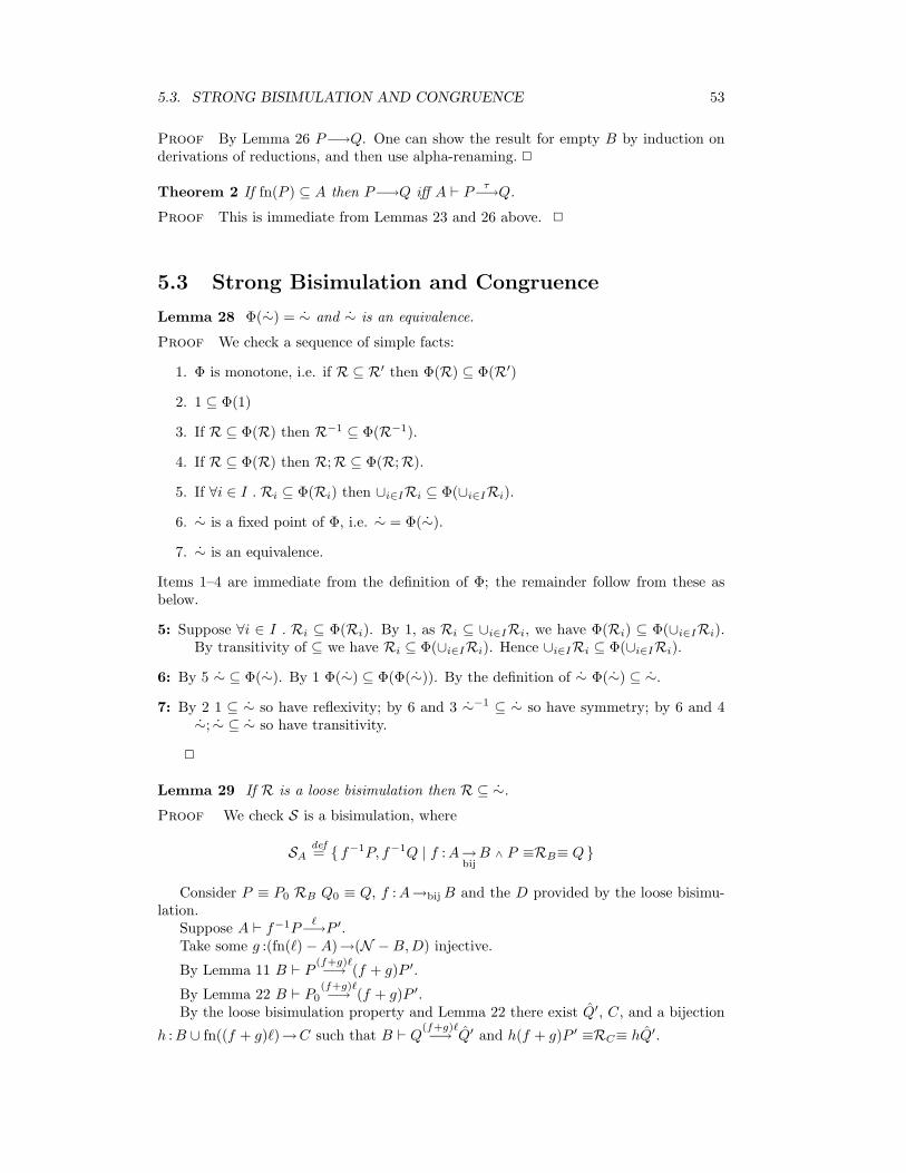
5.3. STRONG BISIMULATION AND CONGRUENCE 53
Proof By Lemma 26 P−→Q. One can show the result for empty B by induction onderivations of reductions, and then use alpha-renaming. 2
Theorem 2 If fn(P ) ⊆ A then P−→Q iff A ` P τ−→Q.
Proof This is immediate from Lemmas 23 and 26 above. 2
5.3 Strong Bisimulation and Congruence
Lemma 28 Φ(∼) = ∼ and ∼ is an equivalence.
Proof We check a sequence of simple facts:
1. Φ is monotone, i.e. if R ⊆ R′ then Φ(R) ⊆ Φ(R′)
2. 1 ⊆ Φ(1)
3. If R ⊆ Φ(R) then R−1 ⊆ Φ(R−1).
4. If R ⊆ Φ(R) then R;R ⊆ Φ(R;R).
5. If ∀i ∈ I . Ri ⊆ Φ(Ri) then ∪i∈IRi ⊆ Φ(∪i∈IRi).
6. ∼ is a fixed point of Φ, i.e. ∼ = Φ(∼).
7. ∼ is an equivalence.
Items 1–4 are immediate from the definition of Φ; the remainder follow from these asbelow.
5: Suppose ∀i ∈ I . Ri ⊆ Φ(Ri). By 1, as Ri ⊆ ∪i∈IRi, we have Φ(Ri) ⊆ Φ(∪i∈IRi).By transitivity of ⊆ we have Ri ⊆ Φ(∪i∈IRi). Hence ∪i∈IRi ⊆ Φ(∪i∈IRi).
6: By 5 ∼ ⊆ Φ(∼). By 1 Φ(∼) ⊆ Φ(Φ(∼)). By the definition of ∼ Φ(∼) ⊆ ∼.
7: By 2 1 ⊆ ∼ so have reflexivity; by 6 and 3 ∼−1 ⊆ ∼ so have symmetry; by 6 and 4∼; ∼ ⊆ ∼ so have transitivity.
2
Lemma 29 If R is a loose bisimulation then R ⊆ ∼.
Proof We check S is a bisimulation, where
SAdef= { f−1P, f−1Q | f :A→
bijB ∧ P ≡RB≡ Q }
Consider P ≡ P0 RB Q0 ≡ Q, f :A→bijB and the D provided by the loose bisimu-lation.
Suppose A ` f−1P`−→P ′.
Take some g :(fn(`)−A)→(N −B,D) injective.
By Lemma 11 B ` P (f+g)`−→ (f + g)P ′.
By Lemma 22 B ` P0(f+g)`−→ (f + g)P ′.
By the loose bisimulation property and Lemma 22 there exist Q′, C, and a bijection
h :B ∪ fn((f + g)`)→C such that B ` Q(f+g)`−→ Q′ and h(f + g)P ′ ≡RC≡ hQ′.

54 CHAPTER 5. METATHEORY: DETAILED PROOFS
By Lemma 11 A ` f−1Q`−→(f + g)−1Q′.
Now h ◦ (f + g) :A ∪ fn(`)→bij C, so P ′ SA∪fn(`) (f + g)−1Q′. 2
Lemma 30 (Injective Substitution – Bisimulation) If P ∼A Q and f :A→B isinjective then fP ∼B fQ.
Proof We check
RB= { fP1, fP2 | f :A→injB ∧ P1∼AP2 }
is a bisimulation.Suppose B ` fP1
`′−→Q′1. By Lemma 13 one of the following holds.
1. there exist `, Q1, g :(fn(`)−A)→bij B such that B ∩B = ∅ and `′ = (f + g)(`) and
A ` P1`−→Q1 and Q′1 = (f + g)Q1.
By bisimulation A ` P2`−→Q2 and Q1∼A∪fn(`)Q2.
By Lemma 11 B ` fP2`′−→(f + g)Q2.
Finally (f + g)Q1 RB∪fn(`′) (f + g)Q2.
2. there exist x ∈ A, y 6∈ A, z ∈ B − ran(f) and Q1 such that `′ = f (x )z andA ` P1
xy−→Q1 and Q′1 = (f + {z/y})Q1.
By bisimulation A ` P2xy−→Q2 and Q1∼A,yQ2.
By Lemma 11 (for the pair of functions f :A→B−z, g :{y}→{z}) we have B − z `fP2
`′−→(f + {z/y})Q2.
By Lemma 12 B ` fP2`′−→(f + {z/y})Q2.
Finally (f + {z/y})Q1 RB (f + {z/y})Q2.
2
Lemma 31 (Congruence – Par and New) If P ∼A,B P ′ and Q ∼A,B Q′ thennew B in (P |Q) ∼A new B in (P ′ |Q′).Proof Let RA= {new B in (P |Q),new B in (P ′ |Q′) | P ∼A,B P ′ ∧ Q ∼A,B Q′ }.We check R is a loose bisimulation (omitting symmetric cases).
Suppose A ` new B in (P |Q) `−→R and fn(`) ∩B = ∅.By Lemma 18 one of the following holds.
1. There exists R such that A,B ` P |Q `−→R and R ≡ new B in R By Lemma 16.3either
3a (Par) there exists P such that fn(Q) ⊆ (A,B), (A,B) ` P `−→P and R ≡P |Q.
By the definition of bisimulation we have P ′ such that A,B ` P ′ `−→P ′ andP ∼(A,B)∪fn(`) P
′.
By (Par) A,B ` P ′ |Q′ `−→P ′ |Q′.By (Res) A ` new B in (P ′ |Q′) `−→new B in (P ′ |Q′).Now, weakening by Lemma 30 gives Q ∼(A,B)∪fn(`) Q
′, soR ≡ new B in P |Q RA∪fn(`) new B in (P ′ |Q′).

5.3. STRONG BISIMULATION AND CONGRUENCE 55
3b (Com) there exist x, v, P and Q such that ` = τ , (A,B) ` P xv−→P , (A,B) `Q
xv−→Q, and R ≡ new {v} − (A,B) in (P | Q).
By the definition of bisimulation we have P ′ and Q′ such that A,B ` P ′ xv−→P ′,A,B ` Q′ xv−→Q′, P ∼(A,B)∪{x,v} P
′, and Q ∼(A,B)∪{x,v} Q′.
By (Com) and (Res) A ` new B in P ′ |Q′ τ−→R′where R′ = new B in new {v} −A,B in P ′ | Q′.Finally, we have R ≡RA R′.
2. there exist y ∈ A, x 6∈ A, x ∈ B and R such that ` = yx , A,B ` P |Q yx−→R, andR ≡ {x/x}new B − x in R.
We have P such that A,B ` P yx−→P and R ≡ P |Q.
By the definition of bisimulation we have P ′ such that A,B ` P ′ yx−→P ′ and P ∼A,BP ′.
By (Par), (Open) and (Res) A ` new B in P ′ |Q′ yx−→R′′ whereR′′ = new B − x in P ′ | Q′.
By Lemma 11 A ` new B in P ′ |Q′ yx−→{x/x}R′′.Finally, we have R ≡ {x/x}new B − x in P |Q and (new B − x in P |Q) RA,x(new B − x in P ′ |Q′).
2
Lemma 32 (Asynchrony) If A ` P zv−→Q zv−→R then A ` P τ−→new {v} −A in R.
Proof By Lemma 24 P ≡ new {v} −A in (zv |Q). By Lemma 25 there exist B, p,Q1
and Q2 such that B ∩ (A ∪ fn(zv) ∪ fn(zv)) = {}, Q ≡ new B in (zp.Q1 |Q2) and R ≡new B in ({v/p}Q1 |Q2). Combining these P ≡ new {v} −A in new B in (zv | zp.Q1 |Q2),so by the transition rules A ` P τ−→new {v} −A in R. 2
Lemma 33 (Substitution – Bisimulation) If P ∼A Q and σ :A→B then σP ∼BσQ.
Proof Define R by
RB = {σP, σP ′ | ∃A . σ :A→B ∧ P ∼A P ′ }
We check R is a bisimulation up to ≡. Suppose B ` σP `−→Q.
Case ` = xv with v ∈ B.
By Lemma 24 σP ≡ xv |Q.
There exist x, v and Q (all above A) such that P ≡ x v | Q, σx = x, σv = v, andσQ = Q.
Note that A ∪ {x, v} = A and B ∪ {x, v} = B.
By the transition rules A ` P x v−→Q.
By P ∼A P ′ we have Q′ such that A ` P ′ x v−→Q′ and Q ∼A Q′.
By Lemma 10 B ` σP ′ xv−→σQ′.It remains only to note Q = σQ RB σQ′.

56 CHAPTER 5. METATHEORY: DETAILED PROOFS
Case ` = xv with v 6∈ B.
By Lemma 24 σP ≡ new v in xv |Q.
There exist x ∈ A, v 6∈ A and Q above A, v such that P ≡ new v in x v | Q, σx = x,and σQ = Q, where σ = σ + (v 7→ v) :A, v→B, v.
By the transition rules A ` P x v−→Q.
By P ∼A P ′ we have Q′ such that A ` P ′ x v−→Q′ and Q ∼A∪{x,v} Q′.
By Lemma 10 B ` σP ′ xv−→σQ′.
It remains only to note Q = σQ RB∪{x,v} σQ′.
Case ` = xv .
By Lemma 25 there exist C, p,Q1 and Q2 such that C ∩ (B ∪ fn(xv)) = {}, σP ≡new C in (xp.Q1 |Q2) and Q ≡ new C in ({v/p}Q1 |Q2).
There exist x ∈ A, a set C disjoint from A, φ : C→C a bijection, p 6∈ A, C, Q1
above A, C, p, and Q2 above A, C such that P ≡ new C in (x p.Q1 | Q2), σx = x,(σ + φ+ (p 7→ p))Q1 = Q1, (σ + φ)Q2 = Q2.
If v ∈ ran(σ) then take some v ∈ A such that σv = v and let σ = σ :A→B,otherwise take some v 6∈ A, C and let σ = σ + (v 7→ v) :A, v→B ∪ {v}.
By the transition rules A ` P x v−→new C in ({v/p}Q1 | Q2).
By P ∼A P ′ we have Q′ such that A ` P ′ x v−→Q′ and
new C in ({v/p}Q1 | Q2) ∼A∪{x,v} Q′
By Lemma 10 B ` σP ′ xv−→σQ′.
Now
Q ≡ new C in ({v/p}Q1 |Q2)= σnew C in ({v/p}Q1 | Q2)
RB∪{x,v} σQ′
Case ` = τ .
By Lemma 27 there exist C, x, v, p,Q1, Q2 such that C∩(B∪A) = ∅, p 6∈ B∪A∪C,σP ≡ new C in (xv | xp.Q1 |Q2) and Q ≡ new C in ({v/p}Q1 |Q2).
There exist x, ˆx and v in A,C, Q1 above A,C, p, and Q2 above A,C such thatP ≡ new C in (x v | ˆxp.Q1 | Q2), (σ + idC)x = x, (σ + idC)ˆx = x, (σ + idC)v = v,(σ + idC,p)Q1 = Q1, (σ + idC)Q2 = Q2. Note that either v = v ∈ C or else v ∈ B,v ∈ A and σ(v) = v.
Case x = ˆx By the transition rulesA ` P τ−→Q where Q = new C in ({v/p}Q1 | Q2).Note σQ ≡ Q.By P ∼A P ′ we have Q′ such that A ` P ′ τ−→Q′ and Q ∼A Q′.By Lemma 10 B ` σP ′ τ−→σQ′.It remains only to note Q ≡ σQ RB σQ′.

5.3. STRONG BISIMULATION AND CONGRUENCE 57
Case x 6= ˆx As the ranges of σ and idC are disjoint we have x ∈ A and ˆx ∈ A.By the transition rules
A ` P x v−→ new C − {v} in (ˆxp.Q1 | Q2)ˆx v−→ new C − {v} in ({v/p}Q1 | Q2)
By P ∼A P ′ we have Q′ such that
A ` P ′ x v−→ˆx v−→ Q′
and
new C − {v} in ({v/p}Q1 | Q2) ∼A∪{v} Q′
By Lemma 10, taking g = {v/v} if v = v ∈ C and g = ∅ if v ∈ A,
B ` σP ′ xv−→xv−→ (σ + g)Q′
By Lemma 32 B ` σP ′ τ−→new {v} − B in (σ + g)Q′.Case v = v ∈ C. We have
Q ≡ new C in {v/p}Q1 |Q2
≡ new C in {v/p}(σ + idC,p)Q1 |(σ + idC)Q2
≡ σnew C in {v/p}Q1 | Q2
≡ σnew v in new C − v in {v/p}Q1 | Q2
RB σnew v in Q′ Using Lemma 31 for new v in cong≡ new v − B in (σ + g)Q′
Case v ∈ A. We have
Q ≡ new C in {v/p}Q1 |Q2
≡ new C in {v/p}(σ + idC,p)Q1 |(σ + idC)Q2
≡ new C in (σ + idC){v/p}Q1 |(σ + idC)Q2
≡ σnew C in {v/p}Q1 | Q2
RB σQ′
≡ new v − B in (σ + g)Q′
2
Lemma 34 (Congruence – Input Prefix) If P ∼A,pQ and x ∈ A then xp.P ∼Axp.Q.
Proof We check the union of ∼ and the pair (xp.P, xp.Q) at A is a bisimulation upto ≡.
The cases P ∼BQ are routine.Suppose A ` xp.P `−→P ′.By Lemma 16 there exist v such that ` = xv and P ′ ≡ {v/p}P .By (Inp) A ` xp.Q xv−→{v/p}Q.By Lemma 33 {v/p}P ∼A∪{v}{v/p}Q. 2
Theorem 3 Bisimulation ∼ is an indexed congruence.
Proof Immediate from Lemmas 31 and 34. 2

58 CHAPTER 5. METATHEORY: DETAILED PROOFS
5.4 Type Soundness and Subject Reduction
Lemma 35 (Weakening – Values) If Γ ` v :T ′ and x 6∈ dom(Γ) then Γ, x :T ` v :T ′.
Proof By induction on type derivations. 2
Lemma 36 (Weakening – Processes) If Γ ` P proc and x 6∈ dom(Γ) then Γ, x :T `P proc.
Proof By induction on type derivations, using Lemma 35. 2
Lemma 37 (Strengthening – Values) If Γ, x :T ` v :T ′ and x 6∈ fn(v) then Γ `v :T ′.
Proof By induction on type derivations. 2
Lemma 38 (Strengthening – Processes) If Γ, x :T ` P proc and x 6∈ fn(P ) thenΓ ` P proc.
Proof By induction on type derivations , using Lemma 37. 2
Lemma 39 (Type Soundness of Structural Congruence) If P ≡ Q then Γ `P proc iff Γ ` Q proc.
Proof By induction on the derivation of P ≡ Q.
(ParId) Γ ` P | 0 proc iff Γ ` P proc ∧ Γ ` 0 proc iff Γ ` P proc.
(ParComm),(ParAssoc) Similar.
(NewExtrude) P |new x : T in Q ≡ new x : T in (P | Q) with x 6∈ fn(P ).
Take Q and x 6∈ dom(Γ)∪fn(P ) such that P |new x : T in Q = P |new x : T in Qand new x : T in (P |Q) = new x : T in (P | Q). We have
Γ ` P |new x : T in Q proc ⇐⇒ Γ ` P proc ∧ Γ ` new x : T in Q proc⇐⇒ Γ ` P proc ∧ Γ, x :T ` Q proc⇐⇒ Γ, x :T ` P proc ∧ Γ, x :T ` Q proc (∗)⇐⇒ Γ, x :T ` P |Q proc⇐⇒ Γ ` new x : T in P |Q proc
Here (∗) is by Lemmas 36 and 38.
(NewComm) Straightforward.
(CongIn),(CongPar),(CongNew) By the induction hypothesis and the correspond-ing typing rule.
(Refl),(Sym),(Tran) By the induction hypothesis and the corresponding propertiesof iff.
2
Lemma 40 (Injective Substitution – Reductions) If P → Q and f : fn(P )→N isinjective then fP → fQ.
We define well-typed substitutions as follows. Say Γ ` σ : ∆ iff dom(σ) = dom(∆)and ∀x ∈ dom(∆) . Γ ` σ(x) : ∆(x).

5.4. TYPE SOUNDNESS AND SUBJECT REDUCTION 59
Lemma 41 (Good Substitutions) If Γ atomic and Γ ` v :T and ` p :T B ∆ then{v/p} is defined and Γ ` {v/p} : ∆.
Proof By induction on the two typing derivations. Consider the last rule of thepattern judgement.
(Var) ` x :T B x :T . Clearly {v/x} = {x 7→ v}, dom({x 7→ v}) = dom(x :T ), andΓ ` {v/x}x :T .
(Tuple) ` 〈p1 .. pk〉 : 〈T1 .. Tk〉 B ∆1, ..,∆k. As Γ atomic the last rule of the value judge-ment must either be the value (Tuple) rule, with conclusion Γ ` 〈v1 .. vk〉 : 〈T1 .. Tk〉,or the value (Var) rule, with k = 0. In the first case, by the induction hypoth-esis for each i we have {vi/pi} defined and Γ ` {vi/pi} : ∆i. By the definition ofsubstitution {〈v1 .. vk〉/〈p1 .. pk〉} is defined and equal to
⋃i∈1..k{vi/pi}. As for each
i dom({vi/pi}) = dom(∆i), we have dom(⋃i∈1..k{vi/pi}) = dom(∆1, ..,∆k). To
check Γ ` {〈v1 .. vk〉/〈p1 .. pk〉} : ∆1, ..,∆k it remains only to observe that for eachz :T ′ ∈ ∆1, ..,∆k there is an i with z :T ′ ∈ ∆i, hence Γ ` {vi/pi}z :T ′, henceΓ ` (
⋃i∈1..k{vi/pi})z :T ′.
In the second case, by the definition of substitution {〈〉/〈〉} is defined and equal to∅, and Γ ` ∅ : ∅.
Note that this result requires that the range of Γ contains no non-unit tuple types. 2
Lemma 42 (Substitution – Values) If Γ,∆ ` v :T and Γ ` σ : ∆ then Γ ` σv :T .
Proof By induction on the value typing derivation.
(Var) Γ,∆ ` x :T .
Case x :T ∈ Γ. By the second premise the domain of σ coincides with that of ∆and hence is disjoint from Γ, so σ(x) = x, so Γ ` σ(x) :T .
Case x :T ∈ ∆. By the second premise Γ ` σ(x) :T .
(Tuple) Γ,∆ ` 〈v1 .. vk〉 : 〈T1 .. Tk〉. By the induction hypothesis for each i we have Γ `σ(vi) :Ti hence Γ ` σ(〈v1 .. vk〉) : 〈T1 .. Tk〉
2
Lemma 43 (Substitution – Processes) If Γ,∆ ` P proc and Γ ` σ : ∆ then σP isdefined and Γ ` σP proc.
Proof We prove both parts simultaneously by induction on the type derivation forP . For the second part we give two instances of each typing rule; in each case showingthat the premises of the right-hand instance follow from those of the left-hand instance.
(Out)
Out
Γ,∆ ` x : chanTΓ,∆ ` v :TΓ,∆ ` xv proc Out
Γ ` σ(x) : chanTΓ ` σ(v) :T
Γ ` σ(x )σ(v) proc
By Lemma 42 both premises of the right-hand-side instance hold. As Γ ` σ(x) : chanTwe have that σ(x) is a name, so σ(xv) is defined.

60 CHAPTER 5. METATHEORY: DETAILED PROOFS
(In)
In
Γ,∆ ` x : chanT` p :T B ΘΓ,∆,Θ ` P procΓ,∆ ` xp.P proc In
Γ ` σ(x) : chanT` p :T B ΘΓ,Θ ` σ(P ) proc
Γ ` σ(x )p.σ(P ) proc
By Lemma 42 the first premise of the right-hand-side instance holds. The secondis immediate, and clearly Γ,Θ ` σ : ∆, so the third follows from the inductionhypothesis, which also tells us that σP is defined. As Γ ` σ(x) : chanT we havethat σ(x) is a name, so σ(xp.P ) is defined.
(Par)
Par
Γ,∆ ` P procΓ,∆ ` Q proc
Γ,∆ ` P |Q proc Par
Γ ` σP procΓ ` σQ proc
Γ ` σP |σQ proc
The two premises of the right-hand-side instance are immediate from the inductionhypothesis, and σ(P |Q) is defined as σP and σQ are defined.
(Nil)
Nil Γ,∆ ` 0 proc Nil Γ ` 0 proc
Trivial.
(Res)
ResΓ,∆, x : chanT ` P proc
Γ,∆ ` new x : chan T in P proc ResΓ, x : chanT ` σP proc
Γ ` new x : chan T in σP proc
Clearly Γ, x : chanT ` σ : ∆, so the premise follows from the induction hypothesis,which also tells us that σP is defined and hence that σ(new x : chan T in P ) is.
2
Theorem 4 (Subject Reduction) If Γ ` P proc and Γ atomic and P → Q thenΓ ` Q proc.
Proof By induction on the derivation of P → Q.
(Com) Suppose (being cavalier about alpha equivalence) that the names of p are disjointfrom dom(Γ). By the typing rules we have T such that Γ ` c : chanT , Γ ` v :T ,` p :T B ∆, and Γ,∆ ` P proc. By Lemma 41 {v/p} is defined and Γ ` {v/p} : ∆.By Lemma 43 {v/p}P is defined and Γ ` {v/p}P proc.
(Par) By the typing rules we have Γ ` P proc and Γ ` Q proc. By the inductionhypothesis Γ ` P ′ proc. Using the (Par) typing rule Γ ` P ′ |Q proc.
(Res) By the typing rules we have P and x and T0 such that T = chanT0 andnew x : T in P = new x : T in P and x 6∈ dom(Γ) and Γ, x :T ` P proc. ByLemma 40 P → {x/x}P ′. By the induction hypothesis (noting that Γ, x :T atomic)we have Γ, x :T ` {x/x}P ′ proc. By (Res) Γ ` new x : T in {x/x}P ′ proc. Butthen Γ ` new x : T in P ′ proc.
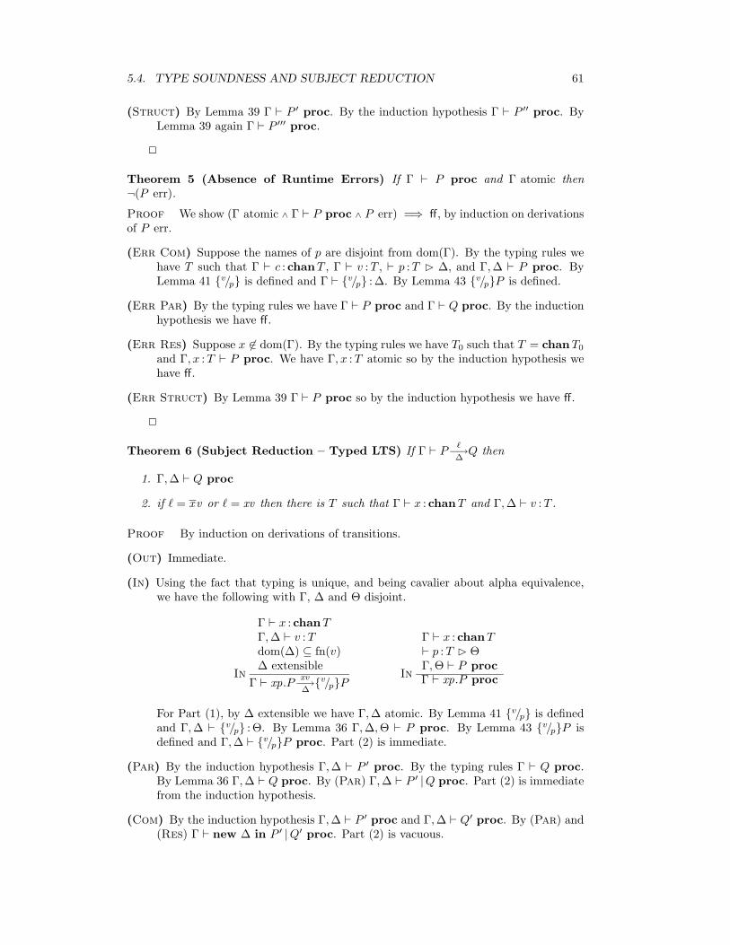
5.4. TYPE SOUNDNESS AND SUBJECT REDUCTION 61
(Struct) By Lemma 39 Γ ` P ′ proc. By the induction hypothesis Γ ` P ′′ proc. ByLemma 39 again Γ ` P ′′′ proc.
2
Theorem 5 (Absence of Runtime Errors) If Γ ` P proc and Γ atomic then¬(P err).
Proof We show (Γ atomic ∧ Γ ` P proc ∧ P err) =⇒ ff, by induction on derivationsof P err.
(Err Com) Suppose the names of p are disjoint from dom(Γ). By the typing rules wehave T such that Γ ` c : chanT , Γ ` v :T , ` p :T B ∆, and Γ,∆ ` P proc. ByLemma 41 {v/p} is defined and Γ ` {v/p} : ∆. By Lemma 43 {v/p}P is defined.
(Err Par) By the typing rules we have Γ ` P proc and Γ ` Q proc. By the inductionhypothesis we have ff.
(Err Res) Suppose x 6∈ dom(Γ). By the typing rules we have T0 such that T = chanT0
and Γ, x :T ` P proc. We have Γ, x :T atomic so by the induction hypothesis wehave ff.
(Err Struct) By Lemma 39 Γ ` P proc so by the induction hypothesis we have ff.
2
Theorem 6 (Subject Reduction – Typed LTS) If Γ ` P `−→∆Q then
1. Γ,∆ ` Q proc
2. if ` = xv or ` = xv then there is T such that Γ ` x : chanT and Γ,∆ ` v :T .
Proof By induction on derivations of transitions.
(Out) Immediate.
(In) Using the fact that typing is unique, and being cavalier about alpha equivalence,we have the following with Γ, ∆ and Θ disjoint.
In
Γ ` x : chanTΓ,∆ ` v :Tdom(∆) ⊆ fn(v)∆ extensible
Γ ` xp.P xv−→∆{v/p}P
In
Γ ` x : chanT` p :T B ΘΓ,Θ ` P procΓ ` xp.P proc
For Part (1), by ∆ extensible we have Γ,∆ atomic. By Lemma 41 {v/p} is definedand Γ,∆ ` {v/p} : Θ. By Lemma 36 Γ,∆,Θ ` P proc. By Lemma 43 {v/p}P isdefined and Γ,∆ ` {v/p}P proc. Part (2) is immediate.
(Par) By the induction hypothesis Γ,∆ ` P ′ proc. By the typing rules Γ ` Q proc.By Lemma 36 Γ,∆ ` Q proc. By (Par) Γ,∆ ` P ′ |Q proc. Part (2) is immediatefrom the induction hypothesis.
(Com) By the induction hypothesis Γ,∆ ` P ′ proc and Γ,∆ ` Q′ proc. By (Par) and(Res) Γ ` new ∆ in P ′ |Q′ proc. Part (2) is vacuous.

62 CHAPTER 5. METATHEORY: DETAILED PROOFS
(Res) By the typing rules T = chanT ′ for some T ′. By the induction hypothesis and(Res) Γ ` new x : T in P ′ proc. Also by the induction hypothesis, if ` = yv or` = yv then there is T ′′ such that Γ, x :T ` y : chanT ′′ and Γ, x :T,∆ ` v :T ′′. ByLemma 35 Γ ` y : chanT ′′ and Γ,∆ ` v :T ′′.
(Open) By the induction hypothesis Γ, x :T,∆ ` P ′ proc so Γ,∆, x :T ` P ′ proc.Also by the induction hypothesis, there is T ′′ such that Γ, x :T ` y : chanT ′′ andΓ, x :T,∆ ` v :T ′′. By x 6= y and Lemma 35 Γ ` y : chanT ′′.
(Struct) By the induction hypothesis and Lemma 39.
2

Bibliography
[AG97] Martın Abadi and Andrew D. Gordon. A calculus for cryptographic protocols:The spi calculus. In Proceedings of the Fourth ACM Conference on Computerand Communications Security, Zurich, pages 36–47. ACM Press, April 1997.
[AP94] R. M. Amadio and S. Prasad. Localities and failures. In P. S. Thiagarajan,editor, Proceedings of 14th FSTTCS. LNCS 880, pages 205–216. Springer-Verlag, 1994.
[BB92] G. Berry and G. Boudol. The chemical abstract machine. Theoretical Com-puter Science, 96:217–248, 1992.
[Bou92] Gerard Boudol. Asynchrony and the π-calculus (note). Rapport de Recherche1702, INRIA Sofia-Antipolis, May 1992.
[CG98] Luca Cardelli and Andrew D. Gordon. Mobile ambients. In Proc. of Founda-tions of Software Science and Computation Structures (FoSSaCS), ETAPS’98,LNCS 1378, pages 140–155, March 1998.
[CS00] Gian Luca Cattani and Peter Sewell. Models for name-passing processes:Interleaving and causal. In Proceedings of LICS 2000: the 15th IEEE Sym-posium on Logic in Computer Science (Santa Barbara), pages 322–333, June2000.
[FG96] Cedric Fournet and Georges Gonthier. The reflexive CHAM and the join-calculus. In Proceedings of the 23rd POPL, pages 372–385. ACM press, Jan-uary 1996.
[FGL+96] Cedric Fournet, Georges Gonthier, Jean-Jacques Levy, Luc Maranget, andDidier Remy. A calculus of mobile agents. In Proceedings of CONCUR ’96.LNCS 1119, pages 406–421. Springer-Verlag, August 1996.
[Fou98] Cedric Fournet. The Join-Calculus: A Calculus for Distributed Mobile Pro-gramming. PhD thesis, Ecole Polytechnique, Paris, 1998.
[Gla90] R. J. van Glabbeek. The linear time – branching time spectrum. In Proceedingsof CONCUR ’90, LNCS 458, pages 278–297, 1990.
[Gla93] R. J. van Glabbeek. The linear time – branching time spectrum II; the seman-tics of sequential systems with silent moves. In Proceedings of CONCUR’93,LNCS 715, pages 66–81, 1993.
[HT91] Kohei Honda and Mario Tokoro. An object calculus for asynchronous com-munication. In Proceedings of ECOOP ’91, LNCS 512, pages 133–147, July1991.
63

64 BIBLIOGRAPHY
[Joi] The join-calculus. Papers and implementations available athttp://pauillac.inria.fr/join/.
[Mil92] Robin Milner. Functions as processes. Journal of Mathematical Structures inComputer Science, 2(2):119–141, 1992.
[Mil99] Robin Milner. Communicating and Mobile Systems: the π-Calculus. Cam-bridge University Press, May 1999.
[MPW92] R. Milner, J. Parrow, and D. Walker. A calculus of mobile processes, Parts I+ II. Information and Computation, 100(1):1–77, 1992.
[MS92] Robin Milner and Davide Sangiorgi. Barbed bisimulation. In Proceedings of19th ICALP. LNCS 623, pages 685–695, 1992.
[Nee89] R. M. Needham. Names. In S. Mullender, editor, Distributed Systems, pages89–101. Addison-Wesley, 1989.
[Nes] Uwe Nestmann. Calculi for mobile processes. Available athttp://move.to/mobility and http://www.cs.auc.dk/mobility/.
[NP96] Uwe Nestmann and Benjamin C. Pierce. Decoding choice encodings. In Pro-ceedings of CONCUR ’96, LNCS 1119, pages 179–194, August 1996.
[Pal97] Catuscia Palamidessi. Comparing the expressive power of the synchronousand the asynchronous π-calculus. In Proceedings of POPL 97, pages 256–265,1997.
[PC98] Catuscia Palamidessi and Ilaria Castellani, editors. EXPRESS ’98: Expres-siveness in Concurrency (Nice, France, September 7, 1998), volume 16.2 ofentcs. Elsevier Science Publishers, 1998.
[Pie98] Benjamin C. Pierce. Type systems for concurrent calculi, September1998. Invited tutorial at CONCUR, Nice, France. Slides available fromhttp://www.cis.upenn.edu/∼bcpierce/.
[PT98] Benjamin C. Pierce and David N. Turner. Pict: A programming lan-guage based on the pi-calculus, March 1998. Version 4.1. Compiler, docu-mentation, demonstration programs, and standard libraries; available fromhttp://www.cis.upenn.edu/∼bcpierce/.
[PT00] Benjamin C. Pierce and David N. Turner. Pict: A programming languagebased on the pi-calculus. In Proof, Language and Interaction: Essays inHonour of Robin Milner. MIT Press, 2000.
[Qua99] P. Quaglia. The π-calculus: notes on labelled semantics. Bulletin of theEATCS, 68, June 1999. Preliminary version as BRICS Report LS-98-4.
[QW98] P. Quaglia and D. Walker. On encoding pπ in mπ. In Proc. 18th FSTTCS,LNCS 1530, pages 42–53. Springer Verlag, 1998.
[RH99] James Riely and Matthew Hennessy. Trust and partial typing in open systemsof mobile agents. In Proceedings of the 26th POPL, San Antonio, January1999. ACM Press.
[San93] Davide Sangiorgi. Expressing Mobility in Process Algebras: First-Order andHigher-Order Paradigms. PhD thesis, University of Edinburgh, 1993.

BIBLIOGRAPHY 65
[Sew97] Peter Sewell. On implementations and semantics of a concurrent programminglanguage. In Proceedings of CONCUR ’97. LNCS 1243, pages 391–405, 1997.
[Sew98] Peter Sewell. Global/local subtyping and capability inference for a dis-tributed π-calculus. In Proceedings of ICALP ’98. LNCS 1443, pages 695–706. Springer-Verlag, July 1998. See also Technical Report 435, University ofCambridge, 1997.
[SV99] Peter Sewell and Jan Vitek. Secure composition of insecure components.In Proceedings of the 12th IEEE Computer Security Foundations Workshop.Mordano, Italy, pages 136–150. IEEE Computer Society, June 1999.
[SV00] Peter Sewell and Jan Vitek. Secure composition of untrusted code: Wrappersand causality types. In Proceedings of CSFW 00: The 13th IEEE Com-puter Security Foundations Workshop., pages 269–284. IEEE Computer Soci-ety, July 2000.
[SWP98] Peter Sewell, Pawe l T. Wojciechowski, and Benjamin C. Pierce. Locationindependence for mobile agents. In Workshop on Internet Programming Lan-guages, Chicago. Springer-Verlag, May 1998. Full version as Technical Report462, University of Cambridge, and in LNCS 1686.
[Tho93] Bent Thomsen. Plain CHOCS. A second generation calculus for higher orderprocesses. Acta Informatica, 30(1):1–59, 1993.
[TLK96] Bent Thomsen, Lone Leth, and Tsung-Min Kuo. A Facile tutorial. In Proceed-ings of CONCUR ’96. LNCS 1119, pages 278–298. Springer-Verlag, August1996.
[Tur96] David N. Turner. The Polymorphic Pi-calculus: Theory and Implementation.PhD thesis, University of Edinburgh, 1996.
[VC98] Jan Vitek and Guiseppe Castagna. Towards a calculus of mobile computa-tions. In Workshop on Internet Programming Languages, Chicago, May 1998.Full version in LNCS 1686.
[Yos96] Nobuko Yoshida. Graph types for monadic mobile processes. In Proceedingsof FSTTCS 96, LNCS, pages 371–386, 1996.