Applied Probabilistic Reasoning: AVade Mecum to Accompany a First

Course in Statistics

Ehsan Bokhari and Lawrence HubertThe University of Illinois

March 23, 2015

1

A Brief Primer on AppliedProbabilistic Reasoning

I think it much more interesting to live with uncertainty than to live withanswers that might be wrong.

– Richard Feynman

Abstract: This initial module of the vade mecum is intended

as an informal introduction to several central ideas in probabilistic

reasoning. The first topic introduced concerns Sally Clark, who was

convicted in England of killing her two children, partially on the ba-

sis of an inappropriate assumption of statistical independence. Next,

the infamous O.J. Simpson murder trial is recalled along with defense

lawyer Johnnie Cochran’s famous dictum: “if it doesn’t fit, you must

acquit.” This last statement is reinterpreted probabilistically and

then used to introduce the two key probabilistic reasoning concepts

of an event being either facilitative or inhibitive of another. Based on

these two notions of facilitation and inhibition, a number of topic ar-

eas are then reviewed in turn: probabilistic reasoning based on data

organized in the form of 2× 2 contingency tables; the Charles Peirce

idea of abductive reasoning; Bayes’ theorem and diagnostic testing;

the fallacy of the transposed conditional; how to interpret probability

and risk and deal generally with probabilistic causation; where the

numbers might come from that are referred to as probabilities and

what they may signify; the misunderstandings that can arise from

relying on nontransparent odds ratios rather than on relative risks;

and finally, how probabilistic causation has been dealt with success-

fully in a federal program to compensate workers exposed to ionizing

radiation and other toxic materials through their involvement with

2

the United States’ nuclear weapons industry. The last section of this

brief primer discusses a set of eleven additional instructional modules

that cover a variety of (other) probabilistic reasoning topics. These

modules are available through a web location given in this last sec-

tion.

Contents

1 Introduction 4

2 Some Initial Basics: The O.J. Simpson Case and

the Legend of Cinderella 7

2.1 Alternative Approaches to Probabilistic Reasoning . . 13

3 Data in the Form of a 2× 2 Contingency Table 17

4 Abductive Reasoning 20

5 Bayes’ Rule (Theorem) 26

5.1 Beware the Fallacy of the Transposed Conditional . . 32

6 Probability of Causation 37

6.1 The Energy Employees Occupational Illness Compen-

sation Program (EEOICP) . . . . . . . . . . . . . . 40

7 The Interpretation of Probability and Risk 44

7.1 Where Do the Numbers Come From that Might Be

Referred to as Probabilities and What Do They Signify 48

7.2 The Odds Ratio: A Statistic that Only a Statistician’s

Mother Could Love . . . . . . . . . . . . . . . . . . 59

3

8 Probabilistic Reasoning and the Prediction of Hu-

man Behavior 63

9 Where to Go From Here 71

10 Appendix: Supreme Court Denial of Certiorari

in Duane Edward Buck v. Rick Thaler, Director,

Texas Department of Criminal Justice, Correc-

tional Institutions Division 81

11 Appendix: Guidelines for Determining the Prob-

ability of Causation and Methods for Radiation

Dose Reconstruction Under the Employees Oc-

cupational Illness Compensation Program Act of

2000 90

1 Introduction

The formalism of thought offered by probability theory is one of the

more useful portions of any beginning course in statistics in helping

promote quantitative literacy. As typically presented, we speak of

an event represented by a capital letter, say A, and the probability

of the event occurring as some number in the range from zero to

one, written as P (A). The value of 0 is assigned to the “impossible”

event that can never occur; 1 is assigned to the “sure” event that will

always occur. The driving condition for the complete edifice of all

probability theory is one single postulate: for two mutually exclusive

events, A and B (where mutual exclusivity implies that both events

cannot occur at the same time), the probability that A or B occurs

4

is the sum of the separate probabilities associated with the events A

and B: P (A or B) = P (A) +P (B). As a final beginning definition,

we say that two events are independent whenever the probability of

occurrence for the joint event, A and B, factors as the product of

the individual probabilities: P (A and B) = P (A)P (B). Intuitively,

two events are independent if knowing that one event has already

occurred doesn’t alter an assessment of the probability of the other

event occurring.1

The idea of statistical independence and the factoring of the joint

event probability immediately provides a formal tool for understand-

ing several historical miscarriages of justice; it also provides a good

introductory illustration for the general importance of correct prob-

abilistic reasoning. Specifically, if two events are not independent,

then the joint probability cannot be generated by a simple product

of the individual probabilities. A fairly recent and well-known judicial

example involving probabilistic (mis)reasoning and the (mis)carriage

of justice, is the case of Sally Clark; she was convicted in England

of killing her two children, partially on the basis of an inappropri-

ate assumption of statistical independence. The purveyor of sta-

tistical misinformation in this case was Sir Roy Meadow, famous for

Meadow’s Law: “ ‘One sudden infant death is a tragedy, two is suspi-

cious, and three is murder until proved otherwise’ is a crude aphorism

but a sensible working rule for anyone encountering these tragedies.”1In somewhat more formal notation, it is common to represent the event “A or B” with

the notation A ∪ B, where “∪” is a set union symbol called “cup.” The event “A andB” is typically denoted by A ∩ B, where “∩” is a set intersection symbol called “cap.”When A and B are mutually exclusive, they cannot occur simultaneously; this is denoted byA ∩B = ∅, the impossible event (using the “empty set” symbol ∅). Thus, when A ∩B = ∅,P (A ∪ B) = P (A) + P (B); also, as a definition, A and B are independent if and only ifP (A ∩B) = P (A)P (B).

5

We quote part of a news release from the Royal Statistical Society

(October 23, 2001):

The Royal Statistical Society today issued a statement, prompted by issuesraised by the Sally Clark case, expressing its concern at the misuse of statisticsin the courts.

In the recent highly-publicised case of R v. Sally Clark, a medical expertwitness drew on published studies to obtain a figure for the frequency ofsudden infant death syndrome (SIDS, or ‘cot death’) in families having someof the characteristics of the defendant’s family. He went on to square thisfigure to obtain a value of 1 in 73 million for the frequency of two cases ofSIDS in such a family.

This approach is, in general, statistically invalid. It would only be validif SIDS cases arose independently within families, an assumption that wouldneed to be justified empirically. Not only was no such empirical justificationprovided in the case, but there are very strong a priori reasons for supposingthat the assumption will be false. There may well be unknown genetic orenvironmental factors that predispose families to SIDS, so that a second casewithin the family becomes much more likely.

The well-publicised figure of 1 in 73 million thus has no statistical basis.Its use cannot reasonably be justified as a ‘ballpark’ figure because the er-ror involved is likely to be very large, and in one particular direction. Thetrue frequency of families with two cases of SIDS may be very much lessincriminating than the figure presented to the jury at trial.

The Sally Clark case will be revisited in a later section as an example

of committing the “prosecutor’s fallacy.” It was this last probabilistic

confusion that lead directly to her conviction and imprisonment.

6

2 Some Initial Basics: The O.J. Simpson Case and the

Legend of Cinderella

The most publicized criminal trial in American history was arguably

the O.J. Simpson murder case held throughout much of 1995 in Su-

perior Court in Los Angeles County, California. The former football

star and actor, O.J. Simpson, was tried on two counts of murder after

the death in June of 1994 of his ex-wife, Nicole Brown Simpson, and

a waiter, Ronald Goldman. Simpson was acquitted controversially

after a televised trial lasting more than eight months.

Simpson’s high-profile defense team, led by Johnnie Cochran, in-

cluded such illuminaries as F. Lee Bailey, Alan Dershowitz, and Barry

Scheck and Peter Neufeld of the Innocence Project. Viewers of the

widely televised trial might remember Simpson not being able to fit

easily into the blood-splattered leather glove that was found at the

crime scene and which was supposedly used in the commission of the

murders. For those who may have missed this high theater, there is

a YouTube video that replays the glove-trying-on part of the trial;

just “google”: OJ Simpson Gloves & Murder Trial Footage

This incident of the gloves not fitting allowed Johnnie Cochran in

his closing remarks to issue one of the great lines of 20th century

jurisprudence: “if it doesn’t fit, you must acquit.” The question

of interest here in this initial module on probabilistic reasoning is

whether one can also turn this statement around to read: “if it fits,

you must convict.” But before we tackle this explicitly, let’s step back

and introduce a small bit of formalism in how to deal probabilistically

with phrases such as “if p is true, then q is true,” where p and q are

stand-in symbols for two (arbitrary) propositions.

7

Rephrasing in the language of events occurring or not occurring,

suppose we have the following correspondences:

glove fits: event A occurs

glove doesn’t fit: event A (the negation of A) occurs

jury convicts: event B occurs

jury acquits: event B (the negation of B) occurs

Johnnie Cochran’s quip of “if it doesn’t fit, you must acquit” gets

rephrased as “if A occurs, then B occurs.” Or stated in the notation

of conditional probabilities, P (B|A) = 1.0; that is, the probability

that B occurs “given that” A has occurred is 1.0 (where this latter

phrase of “given that” is represented by the short vertical line “|”);

in words, we have “a sure thing.”

Although many observers of the O.J. Simpson trial might not as-

cribe to the absolute nature of the Johnnie Cochran statement im-

plied by P (B|A) being 1.0, most would likely agree to the following

modification: P (B|A) > P (B). Here, the occurrence of A (the glove

not fitting) should increase the likelihood of acquittal to somewhere

above the original (or marginal or prior) value of P (B); there is,

however, no specification as to how big an increase there should be

other than it being short of the value 1.0 representing “a sure thing.”

To give a descriptive term for the situation where P (B|A) >

P (B), we will say in a non-causal descriptive manner that A is “fa-

cilitative” of B (that is, there is an increase in the probability of B

occurring over its marginal value of P (B)). When the inequality is

in the opposite direction, and P (B|A) < P (B), we say, again in

a non-causal descriptive sense, that A is “inhibitive” of B (that is,

there is a decrease in the probability of B occurring over its marginal

8

value of P (B)).

Based on the rules of probability, the one phrase of A being facil-

itative of B, P (B|A) > P (B), leads inevitably to a myriad of other

such statements: B is facilitative of A and inhibitive of A; A is facil-

itative of B and inhibitive of B; B is facilitative of A and inhibitive

of A; A is facilitative of B and inhibitive of B.2

To give one example of these latter statements, consider “A being

facilitative of B.” In a formula, this says that P (B|A) > P (B), or

in words, the probability of a conviction (B) given that the glove fits

(A) is increased over the marginal or prior probability of a conviction.

Most would likely agree that this is a reasonable statement; the point

being made here is that once we agree that A is facilitative of B, we

must also agree to statements such as A being facilitative of B.

Although this introductory section is intended primarily to be just

that, introductory, the reader may be interested to see in a more

formal way how the steps would proceed from P (B|A) > P (B) to,2A number of alternative words or phrases could be used in place of the terms “facil-

itative” and “inhibitive.” For instance, one early usage of the phrases “favorable to” (for“facilitative”) and “unfavorable to” (for “inhibitive”) along with demonstrations for all theimplications just summarized, is in Kai-Lai Chung’s “On Mutually Favorable Events” (An-nals of Mathematical Statistics, 13, 1942, 338–349). In an evidentiary context, such as thatdeveloped in detail by Schum (1994), the phrase “positively (or favorably) relevant” couldstand for “facilitative,” and the phrase “negatively (or unfavorably) relevant” could sub-stitute for “inhibitive.” Rule 401 in the Federal Rules of Evidence (FRE) defines evidencerelevance as follows:

Evidence is relevant if

(a) it has any tendency to make a fact more or less probable than it would be without theevidence; and

(b) the fact is of consequence in determining the action.

Nevertheless, as discussed in the next section, just because evidence may be relevant doesn’tautomatically then make it admissible under FRE Rule 403.

9

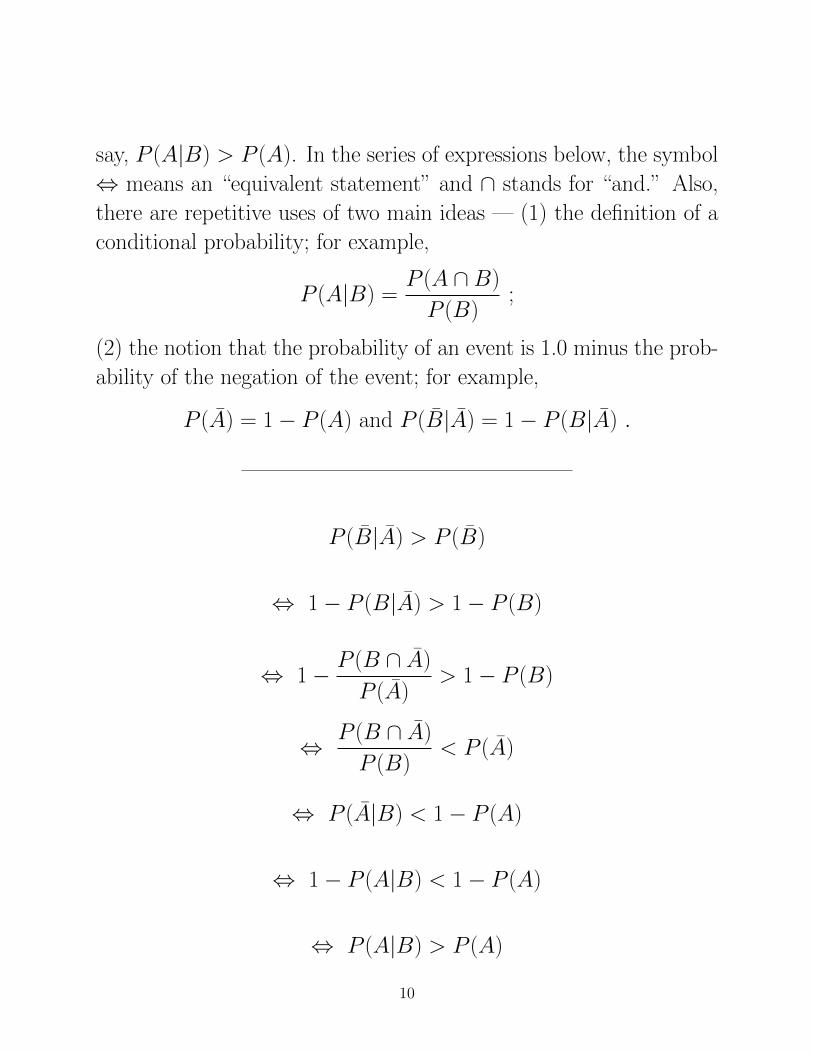
say, P (A|B) > P (A). In the series of expressions below, the symbol

⇔ means an “equivalent statement” and ∩ stands for “and.” Also,

there are repetitive uses of two main ideas — (1) the definition of a

conditional probability; for example,

P (A|B) =P (A ∩B)

P (B);

(2) the notion that the probability of an event is 1.0 minus the prob-

ability of the negation of the event; for example,

P (A) = 1− P (A) and P (B|A) = 1− P (B|A) .

P (B|A) > P (B)

⇔ 1− P (B|A) > 1− P (B)

⇔ 1− P (B ∩ A)

P (A)> 1− P (B)

⇔ P (B ∩ A)

P (B)< P (A)

⇔ P (A|B) < 1− P (A)

⇔ 1− P (A|B) < 1− P (A)

⇔ P (A|B) > P (A)

10

In the language of probability theory, and as noted above in the

Sally Clark case, two events A and B are said to be “independent”

if the probability of the joint event, A ∩ B, factors into the two

(marginal) probabilities of A and of B. Or, to restate the formal

definition: the events A and B are independent if and only if

P (A ∩B) = P (A)P (B)

Using the definition of a conditional probability, A and B are then

independent if and only if

P (A|B) =P (A)P (B)

P (B)= P (A)

or

P (B|A) =P (A)P (B)

P (A)= P (B)

In words, A and B are independent if and only if A (or B) is neither

inhibitive nor facilitative of B (or A).

To give another illustration of how probabilistic reasoning might

reasonably operate, we go back to the legend of Cinderella and make

one slightly risque modification. On her hurried way out of the castle

just before midnight, Cinderella drops the one glass slipper (but say,

she holds on to the other one) and loses all of her fitted clothes and

jewelry including tiara, bra, panties, and so on. When the Prince

sets off to find Cinderella, the following events are of interest:

slipper fits: event A occurs

slipper doesn’t fit: event A (the negation of A) occurs

person is Cinderella: event B occurs

11

person is not Cinderella: event B (the negation of B) occurs

As in the Johnnie Cochran context, the occurrence of the event

A (that the slipper fits) increases the likelihood that event B occurs

(that the person is Cinderella) over the prior probability of this par-

ticular individual being Cinderella. But in our risque version of the

legend, the Prince also has an array of fitted jewelry and clothes that

also could be tried on sequentially, with each fitting item being itself

facilitative of the event B of being Cinderella. Although one may

never reach a “sure thing” and have Cinderella identified “beyond a

shadow of a doubt,” the sequential weight-of-the-evidence may lead

to something at least “beyond a reasonable doubt”; or stated in other

words, the cumulative probability of the event B (of being Cinderella)

increases steadily with each newly fitting item.

The Cinderella saga we have laid out may be akin to what occurs

in criminal cases where a conviction is obtained when the weight-of-

the-evidence has reached a standard of “beyond a reasonable doubt.”

The tougher standard of “beyond a shadow of a doubt” may be

attainable only when there is a proverbial “smoking gun.” In Cin-

derella’s case, this “smoking gun” might amount to producing the ex-

act matching slipper that she held onto that night. For the O.J. Simp-

son case, it’s unclear whether there could have ever been a “smoking

gun” produced; even the available DNA evidence was discounted be-

cause of possible police tampering. If the blood-soaked Bruno Magli

shoes had ever been found and if they had fit O.J. Simpson perfectly,

then maybe — but then again, maybe not.

12

2.1 Alternative Approaches to Probabilistic Reasoning

The approach taken thus far to the basics of applied probabilistic

reasoning has been rather simple. Given events A and A and B

and B, the discussion has been framed merely as one event being

facilitative or inhibitive (or neither) of another event, and without

any particular causal language imposed. As might be expected, all

this can be made more complicated. For example, we begin by in-

troducing likelihood ratios. If an event A is facilitative of B, then

P (B|A) > P (B); but, also, A must then be inhibitive of B or

P (B|A) < P (B). The fraction, P (B|A)P (B|A)

, is called a likelihood ratio,

and must in this case be greater than 1.0 because of the inequality

P (B|A) > P (B) > P (B|A).

In a later section the all-powerful Bayes’ theorem will be intro-

duced and discussed in some detail. Although we won’t do so in that

section, an alternative version of Bayes’ theorem could be given in

the form of posterior odds being equal to a likelihood ratio times

the prior odds. Remembering that odds are defined by the ratio of

the probability of an event to the probability of the complement, the

formal statement would be:

(P (A|B)

P (A|B)) = (

P (B|A)

P (B|A))× (

P (A)

P (A))

or (posterior odds of A) = (likelihood)×(prior odds of A). In words,

when A is facilitative of B, and thus, the likelihood, P (B|A)P (B|A)

, is greater

than 1.0, and given that the event B occurs, the posterior odds of

A occurring is greater than the prior odds of A occurring. In an

13

analogous manner, we could also derive the form

(P (B|A)

P (B|A)) = (

P (A|B)

P (A|B))× (

P (B)

P (B))

And, again in words, given that the event A occurs, the posterior

odds of B occurring is greater than the prior odds of B occurring.

These two equivalent forms of Bayes’ theorem appear regularly in

the judgment and decision making literature whenever the discus-

sion turns to the reliability (or unreliability, as the case might be)

of eyewitness testimony. To illustrate this numerically with a rather

well-known type of example, we paraphrase a presentation from De-

vlin and Lorden (2007, pp. 83–85) involving taxi cabs:

A certain town has two taxi companies, Blue Cabs and Black

Cabs, having, respectively, 15 and 75 taxis. One night when all the

town’s 90 taxis were on the streets, a hit-and-run accident occurred

involving a taxi. A witness sees the accident and claims a blue taxi

was responsible. At the request of the police, the witness underwent a

vision test with conditions similar to those on the night in question,

indicating the witness could successfully identify the taxi color 4

times out of 5. So, the question: which company is the more likely

to have been involved in the accident?

If we let B be the event that the witness says the hit-and-run taxi

is blue, and A the event that the true culprit taxi is blue, the following

probabilities hold: P (A) = 15/90; P (A) = 75/90; P (B|A) = 4/5;

and P (B|A) = 1/5. Thus, the posterior odds are 4 to 5 that the true

taxi was blue: [P (A|B)/P (A|B)] = [(15/90)/(75/90)][(4/5)/(1/5)] ≈4 to 5. In other words, the probability that the culprit taxi is blue

14

is 4/9 ≈ 44%. We note that this latter value is much smaller than

the probability (of 4/5 = 80%) that the eyewitness could correctly

identify a blue taxi when presented with one. This effect is due to the

prior odds ratio reflecting the prevalence of black rather than blue

taxis on the street.

Another approach to certain aspects of probabilistic reasoning that

is in contrast to inductive generalization (which argues from partic-

ular cases to a generalization) is through a “statistical syllogism”

which argues from a generalization that is true for the most part

to a particular case. As an example, consider the following three

statements:

1) Almost all people are taller than 26 inches

2) Larry is a person

3) Therefore, Larry is almost certainly taller than 26 inches

Statement 1) (the major premise) is a generalization and the argu-

ment tries to elicit a conclusion from it. In contrast to a deductive

syllogism, the premise merely supports the conclusion rather than

strictly implying it. So, it is possible for the premise to be true and

the conclusion false but that is not very likely.

One particular statistical syllogism justifies the common under-

standing of a confidence interval as containing the true value of the

parameter in question with a high degree of certainty. When we teach

beginning statistics with an eye toward preciseness, the confidence

interval discussion might be given as follows: (1) “if this particular

confidence interval construction method were repeated for multiple

samples, the collection of all such random intervals would encompass

15

the true population parameter, say, 95% of the time”; (2) “this is

one such constructed interval”; (3) “it is very likely that this interval

contains the true population value.”

The use of statistical syllogisms must obviously be done with care

so that we don’t inappropriately judge individuals only as members

of some group or category and ignore those characteristics that might

“set them apart.” For instance, the Federal Rules of Evidence, Rule

403, implicitly excludes the use of base rates that would be more prej-

udicial than probative (that is, having value as legal proof). Exam-

ples of such exclusions abound but generally involve some judgment

as to which types of demographic groups commit which crimes and

which ones don’t. Rule 403 follows:

Rule 403. Exclusion of Relevant Evidence on Grounds of Prejudice, Confu-sion, or Waste of Time: Although relevant, evidence may be excluded if itsprobative value is substantially outweighed by the danger of unfair prejudice,confusion of the issues, or misleading the jury, or by considerations of unduedelay, waste of time, or needless presentation of cumulative evidence.

Particularly egregious violations of Rule 403 have been ongoing for

some time in Texas capital murder cases. As one recent and perni-

cious example, a psychologist, Walter Quijano, has regularly testified

that because a defendant is black, there is an increased probability of

future violence; or in our event language, the event of being black is

facilitative of the occurrence of a future event (or act) of violence. We

give a redaction in an appendix of the recent Supreme Court case

of Duane Edward Buck v. Rick Taylor (2011), where the defen-

dant, Duane Edward Buck, was attempting to avoid the imposition

of a death penalty sentence. Buck’s lawyers argued that the death

penalty should be lifted because Quijano stated at Buck’s trial that

16

because he was black, there was an increased probability he would

engage in future acts of violence. In Texas capital murder cases, such

predictions of future dangerous behavior are needed to have a death

penalty imposed. The Supreme Court refused to hear the case (that

is, to grant what is called certiorari), not because Buck didn’t have

a case of prejudicial racial evidence being introduced (in violation

of Rule 403), but because, incredibly, Quijano was a witness for the

defense (that is, for Buck).

3 Data in the Form of a 2× 2 Contingency Table

The introduction just given to some elementary ideas in probabilistic

reasoning was phrased in terms of events A and A and their rela-

tion to the events B and B. This discussion can be extended to

frequency distributions, and particularly to those defined by cross-

classifications of individuals according to the events A and A, and

B and B. Organizing the available data in the form of 2× 2 tables

helps facilitate the use of several different approaches to the inter-

pretation of the data – much like Sherlock Holmes looking at all the

data details, and then making conjectures that could then be verified

(or not).

To give a numerical illustration that will be carried through for

awhile, we adopt data provided by Gerd Gigerenzer, Calculated

Risks (2002, pp. 104–107) on a putative group of 10,000 individuals

cross-classified as to whether a Fecal Occult Blood Test (FOBT) is

positive [B: +FOBT] or negative [B: −FOBT], and the presence of

Colorectal Cancer [A: +CC] or its absence [A: −CC]:

17

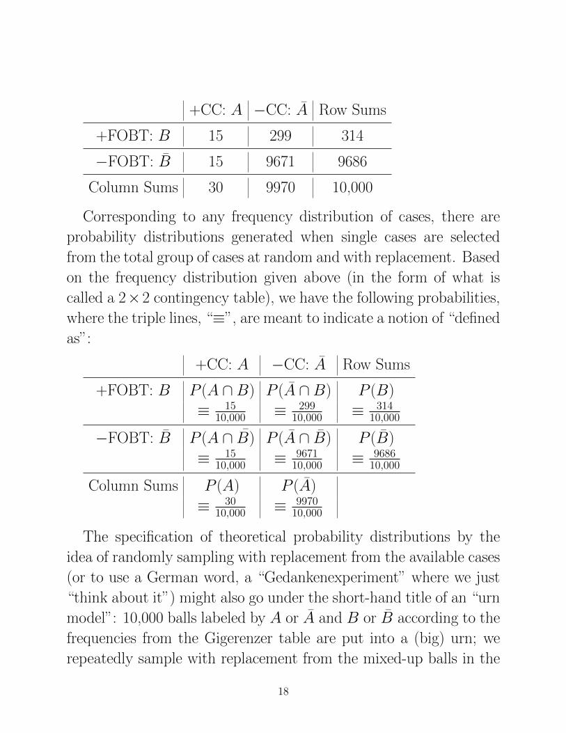
+CC: A −CC: A Row Sums

+FOBT: B 15 299 314

−FOBT: B 15 9671 9686

Column Sums 30 9970 10,000

Corresponding to any frequency distribution of cases, there are

probability distributions generated when single cases are selected

from the total group of cases at random and with replacement. Based

on the frequency distribution given above (in the form of what is

called a 2×2 contingency table), we have the following probabilities,

where the triple lines, “≡”, are meant to indicate a notion of “defined

as”:

+CC: A −CC: A Row Sums

+FOBT: B P (A ∩B) P (A ∩B) P (B)

≡ 1510,000 ≡ 299

10,000 ≡ 31410,000

−FOBT: B P (A ∩ B) P (A ∩ B) P (B)

≡ 1510,000 ≡ 9671

10,000 ≡ 968610,000

Column Sums P (A) P (A)

≡ 3010,000 ≡ 9970

10,000

The specification of theoretical probability distributions by the

idea of randomly sampling with replacement from the available cases

(or to use a German word, a “Gedankenexperiment” where we just

“think about it”) might also go under the short-hand title of an “urn

model”: 10,000 balls labeled by A or A and B or B according to the

frequencies from the Gigerenzer table are put into a (big) urn; we

repeatedly sample with replacement from the mixed-up balls in the

18

urn to generate a sample from the underlying theoretical distribution

just defined in the 2× 2 table of probabilities given above.3

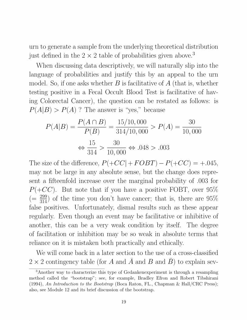
When discussing data descriptively, we will naturally slip into the

language of probabilities and justify this by an appeal to the urn

model. So, if one asks whether B is facilitative of A (that is, whether

testing positive in a Fecal Occult Blood Test is facilitative of hav-

ing Colorectal Cancer), the question can be restated as follows: is

P (A|B) > P (A) ? The answer is “yes,” because

P (A|B) =P (A ∩B)

P (B)=

15/10, 000

314/10, 000> P (A) =

30

10, 000

⇔ 15

314>

30

10, 000⇔ .048 > .003

The size of the difference, P (+CC|+FOBT )−P (+CC) = +.045,

may not be large in any absolute sense, but the change does repre-

sent a fifteenfold increase over the marginal probability of .003 for

P (+CC). But note that if you have a positive FOBT, over 95%

(= 299314) of the time you don’t have cancer; that is, there are 95%

false positives. Unfortunately, dismal results such as these appear

regularly. Even though an event may be facilitative or inhibitive of

another, this can be a very weak condition by itself. The degree

of facilitation or inhibition may be so weak in absolute terms that

reliance on it is mistaken both practically and ethically.

We will come back in a later section to the use of a cross-classified

2× 2 contingency table (for A and A and B and B) to explain sev-3Another way to characterize this type of Gedankenexperiment is through a resampling

method called the “bootstrap”; see, for example, Bradley Efron and Robert Tibshirani(1994), An Introduction to the Bootstrap (Boca Raton, FL., Chapman & Hall/CRC Press);also, see Module 12 and its brief discussion of the bootstrap.

19

eral concepts and anomalies in diagnostic testing and related areas.

Even though we will speak in terms of probabilities and conditional

probabilities, these are typically obtained from frequencies and an

underlying urn model. This general way of developing the descrip-

tive statistics (or what we might label as descriptive probabilities) is

referred to as using “natural frequencies” by Gigerenzer and others.

4 Abductive Reasoning

An alternative strategy to explain what it means for certain events

to be inhibitive or facilitative for other events is through the idea

of abductive reasoning or inference introduced by Charles Peirce in

the late 19th century (for an extensive discussion of Peirce’s life and

work, consult the Wikipedia entry for Charles Sanders Peirce). We

begin by providing Peirce’s beanbag analogy to distinguish between

the three reasoning modes of deduction, induction, and abduction:4

Deduction

(Step 1) Rule: All the beans from this bag are white

(Step 2) Case: These beans are from this bag

Therefore,

(Step 3) Result: These beans are white

Induction

(Step 1) Case: These beans are from this bag

(Step 2) Result: These beans are white4These distinctions between modes of reasoning made by examples such as this one are

available in much of Peirce’s writing; a particularly accessible source for this particular bean-bag illustration is C.S. Peirce, “Deduction, Induction, and Hypothesis” (Popular ScienceMonthly, 13, 1878, 470–482).

20

Therefore,

(Step 3) Rule: All the beans from this bag are white

Abduction

(Step 1) Rule: All the beans from this bag are white

(Step 2) Result: These beans are white

Therefore,

(Step 3) Case: These beans are from this bag

Abduction is a form of logical inference that goes from an obser-

vation to a hypothesis that accounts for the observation and which

explains the relevant evidence. Peirce first introduced the term “ab-

duction” as “guessing” and said that to abduce a hypothetical ex-

planation, say a: these beans are from this bag, from an observed

circumstance, say b: these beans are white, is to surmise that “a”

may be true because then “b” would be a matter of course. Thus, to

abduce “a” from “b” involves determining that “a” is sufficient (or

nearly sufficient) for “b” to be true, but not necessary for “b” to be

true.

As another example, suppose we observe that the lawn is wet. If

it had rained last night, it would be unsurprising that the lawn is

wet; therefore, by abductive reasoning the possibility that it rained

last night is reasonable. Or, stated in our language of events being

facilitative, the event of the lawn being wet (event A) is facilitative

of it raining last night (event B): P (B|A) > P (B). Obviously,

abducing rain last night from the evidence of a wet lawn could lead

to a false conclusion – even in the absence of rain, some other process

such as dew or automatic lawn sprinklers may have resulted in the

wet lawn.

21

The idea of abductive reasoning is somewhat counter to how we

introduce logical considerations in our beginning statistics courses

that revolve around the usual “if p, then q” statements, where p

and q are two propositions. To give a simple example, we might

let p be “the animal is a Yellow Labrador Retriever,” and q, “the

animal is in the order Carnivora.” Continuing, we note that if the

statement “if p, then q” is true (which it is), then logically, so must

be the contrapositive of “if not q, then not p”; that is, if “the animal

is not in the order Carnivora,” then “the animal is not a Yellow

Labrador Retriever.” However, there are two fallacies awaiting the

unsuspecting:

denying the antecedent: if not p, then not q (if “the animal is not

a Yellow Labrador Retriever,” then “the animal is not in the order

Carnivora”);

affirming the consequent: if q, then p (if “the animal is in the order

Carnivora,” then “the animal is a Yellow Labrador Retriever”).

Also, when we consider definitions given in the form of “p if and only

if q,” (for example, “the animal is a domesticated dog” if and only if

“the animal is a member of the subspecies Canis lupus familiaris”),

or equivalently, “p is necessary and sufficient for q,” these separate

into two parts:

“if p, then q” (that is, p is a sufficient condition for q);

“if q, then p” (that is, p is a necessary condition for q).

So, for definitions, the two fallacies are not present.

In a probabilistic context, we reinterpret the phrase “if p, then q”

as B being facilitative of A; that is, P (A|B) > P (A), where p is

identified with B and q with A. With such a probabilistic reinter-

pretation, we no longer have the fallacies of denying the antecedent

22

(that is, P (A|B) > P (A)), or of affirming the consequent (that is,

P (B|A) > P (B)); all of these are now necessary consequences of

the first statement that B is facilitative of A.

In reasoning logically about some situation, it would be rare to

have a context that would be so cut and dried as to lend itself to

the simple logic of “if p, then q,” and where we could look for the

attendant fallacies to refute some causal claim. More likely, we are

given problems characterized by fallible data, and subject to other

types of probabilistic processes. For example, even though someone

may have a genetic marker that has a greater presence in individuals

who have developed some disease (for example, breast cancer and a

mutation in the BRAC1 gene), it is not typically an unadulterated

causal necessity. In other words, it is not true that “if you have

the marker, then you must get the disease.” In fact, many of these

situations might be best reasoned through using our simple 2 × 2

tables; A and A denote the presence/absence of the marker; B and B

denote the presence/absence of the disease. Assuming A is facilitative

of B, we could go on to ask about the strength of the facilitation by

looking at, say, the difference, P (B|A)−P (B), or possibly, the ratio,

P (B|A)/P (B).

As developed in detail by Schum (1994) and others, such probabil-

ity differences and ratios (as well as various other transformations)

are considered important in defining what might be called measures

of “inferential force.” Our discussion will be confined to these kinds of

simple differences and ratios and to rather uncomplicated statements

about their relative sizes. In the context of genetics, for example, the

conditional probability, P (A|B), is typically reported by itself; this

is called “penetrance” – the probability of disease occurrence given

23

the presence of the marker. A fairly recent and high profile instance

of the BRAC1 mutation being assessed as strongly facilitative of

breast cancer (that is, having high “penetrance”) was for the actress

Angelina Jolie, who opted for a prophylactic double mastectomy to

reduce her chances of contracting breast cancer. A few excerpts fol-

low from her Op-Ed article, “My Medical Choice,” that appeared in

the New York Times (May 14, 2013):

My mother fought cancer for almost a decade and died at 56. She heldout long enough to meet the first of her grandchildren and to hold them inher arms. But my other children will never have the chance to know her andexperience how loving and gracious she was.

We often speak of “Mommy’s mommy,” and I find myself trying to explainthe illness that took her away from us. They have asked if the same couldhappen to me. I have always told them not to worry, but the truth is I carry a“faulty” gene, BRCA1, which sharply increases my risk of developing breastcancer and ovarian cancer.

My doctors estimated that I had an 87 percent risk of breast cancer anda 50 percent risk of ovarian cancer, although the risk is different in the caseof each woman.

Only a fraction of breast cancers result from an inherited gene mutation.Those with a defect in BRCA1 have a 65 percent risk of getting it, on average.

Once I knew that this was my reality, I decided to be proactive and tominimize the risk as much I could. I made a decision to have a preventivedouble mastectomy. I started with the breasts, as my risk of breast cancer ishigher than my risk of ovarian cancer, and the surgery is more complex.

...I wanted to write this to tell other women that the decision to have a

mastectomy was not easy. But it is one I am very happy that I made. Mychances of developing breast cancer have dropped from 87 percent to under5 percent. I can tell my children that they don’t need to fear they will loseme to breast cancer.

The idea of arguing probabilistic causation is, in effect, the notion

24

of one event being facilitative or inhibitive of another. If a collection

of “q” conditions is observed that would be the consequence of a

single “p,” one may be more prone to conjecture the presence of

“p,” much like we could do in the Cinderella example. Although

this process may seem like merely affirming the consequent, in a

probabilistic context this could be referred to as “inference to the

best explanation,” or as we have noted above, an interpretation of

the Charles Peirce notion of abductive reasoning. In any case, with

a probabilistic reinterpretation, the assumed fallacies of logic may

not be such. Moreover, most uses of information in contexts that

are legal (forensic) or medical (through screening), or that might, for

example, involve academic or workplace selection, need to be assessed

probabilistically.5

5The Angelina Jolie decision to have a preventive double mastectomy based on her highprobability of eventually contracting breast cancer seems a most rational choice. Otherforms of prophylactic breast removal, however, are more controversial when based on onlya small probability of cancer arising (or being lethal) in an otherwise healthy breast. Asa case in point, Peggy Orenstein in an article for the New York Times (July 26, 2014),entitled “The Wrong Approach to Breast Cancer,” relates her own story about a cancerrecurrence in a breast that had undergone an earlier lumpectomy and radiation in 1997and that now would have to be removed. The question was whether the otherwise healthybreast should also be removed at the same time, through a procedure called “contralateralprophylactic mastectomy” (CPM). The published evidence for undergoing a CPM showsvirtually no survival benefit from the procedure; but still, the use of CPM is mushrooming.As Orenstein notes, there is a “need to recognize the power of ‘anticipated regret’: howpeople imagine they’d feel if their illness returned and they had not done ‘everything’ tofight it when they’d had the chance. Patients will go to extremes to restore peace of mind,even undergoing surgery that, paradoxically, won’t change the medical basis for their fear.”In a letter to the editor of the New York Times (July 31, 2014), Noreen Sugrue states thepoint particularly well that small or large probabilities are not the sole (or even the major)determinant of personal medical choice:

When a woman is given a diagnosis of cancer, the choices she makes about treatmentare based on a number of risk assessments and subjective probabilities. But perhaps mostimportant, those decisions are made so that the woman can find some peace of mind andmove on with her life.

25

5 Bayes’ Rule (Theorem)

One of the most celebrated mathematical results in all of probability

theory is called Bayes’ theorem (or Bayes’ rule or Bayes’ law). Its

modern formulation has been available since the 1812 Laplace publi-

cation, Theorie analytique des probabilities. In commenting on its

importance, Sir Harold Jeffreys (1973, p. 31) noted that Bayes’ the-

orem “is to the theory of probability what Pythagoras’s theorem is

to geometry.” There are several ways to (re)state and extend Bayes’

theorem but here we only need a form for the event pairs of A and

A, and B and B, however the latter are defined.

To begin, note that

P (A|B) = P (A ∩B)/P (B)

and

P (B|A) = P (A ∩B)/P (A)

These two statements directly lead to

P (A|B)P (B) = P (B|A)P (A)

and the simplest form of Bayes’ theorem:

P (A|B) = P (B|A)(P (A)

P (B))

Thus, if we wish to connect the two conditional probabilities P (A|B)

and P (B|A), the latter must be multiplied by the ratio of the marginal

Any model of decision-making has two sets of inputs: probabilities of outcomes and pref-erences, goals or desires. Divergent choices can be made on the same factual basis expressedin the probabilities that a woman assigns to various outcomes.

The decision to have a mastectomy or a lumpectomy, or remove a seemingly healthy breast,should be a woman’s choice without others second-guessing that a wrong decision was made.

26

(or prior) probabilities, P (A)P (B). Noting that P (B) = P (B|A)P (A) +

P (B|A)P (A), the simplest form of Bayes’ theorem can be rewritten

in a less simple but more common form of

P (A|B) =P (B|A)P (A)

P (B|A)P (A) + P (B|A)P (A)

Bayes’ theorem assumes great importance in assessing the value of

diagnostic screening for the occurrence of rare events. For now we

merely give a generic version of a diagnostic testing context and intro-

duce some associated terms. Two introductory numerical examples

are then given: one is for breast cancer screening through mammog-

raphy; the second involves bipolar disorder screening through the

Mood Disorders Questionnaire.

Suppose we have a test that assesses some relatively rare occur-

rence (for example, disease, ability, talent, terrorism propensity, drug

or steroid usage, antibody presence, being a liar [where the test is a

polygraph]). Let B be the event that the test says the person has

“it,” whatever that may be; A is the event that the person really

does have “it.” Two “reliabilities” are needed:

(a) the probability, P (B|A), that the test is positive if the person

has “it”; this is referred to as the sensitivity of the test;

(b) the probability, P (B|A), that the test is negative if the person

doesn’t have “it”; this is the specificity of the test. The conditional

probability used in the denominator of Bayes’ rule, P (B|A), is merely

1− P (B|A), and is the probability of a “false positive.”

The quantity of prime interest, the positive predictive value (PPV),

is the probability that a person has “it” given that the test says

27

so, P (A|B), and is obtainable from Bayes’ rule using the specificity,

sensitivity, and prior probability, P (A):

P (A|B) =P (B|A)P (A)

P (B|A)P (A) + (1− P (B|A))(1− P (A)).

To understand how well the test does, the facilitative effect of B on A

needs interpretation; that is, a comparison of P (A|B) to P (A), plus

an absolute assessment of the size of P (A|B) by itself. Here, the

situation is usually dismal whenever P (A) is small (such as when

screening for a relatively rare occurrence), and the sensitivity and

specificity are not perfect. Although P (A|B) will generally be greater

than P (A), and thus B facilitative of A, the absolute size of P (A|B)

is commonly so small that the value of the screening may be ques-

tionable.6

As will be discussed in greater detail in Module 4 on diagnostic

testing, there is some debate as to how a diagnostic test should be

evaluated; for example, are test sensitivity and specificity paramount

or should our emphasis instead be on the positive and negative pre-

dictive values? Our view at this point is to argue that sensitivity and

specificity, being properties of the test itself and obtained on persons

known to have or not to have the condition in question, would be of

primary interest when deciding whether to use the test. But once the

diagnostic test results are available, and irrespective of whether they6As the example of Angelina Jolie illustrates, the absolute size of P (A|B) may be large

enough to generate decisive action. When B is the event of a BRAC1 mutation and Athe event of contracting breast cancer, the probability P (A|B) was estimated at .87 for theactress; also, when A is the event of contracting ovarian cancer, the probability estimate forP (A|B) drops to .50; but this is still a “as likely as not” assessment of chances for ovariancancer at some point in her life.

28

are positive or negative, sensitivity and specificity are no longer rele-

vant. For clinical or other applied uses, the main issue is to determine

whether the subject in question has the condition given the observed

test results, and this is measured by the positive and negative pre-

dictive values. In other words, if we knew the status of the subject

so sensitivity and specificity would be relevant, it is unnecessary to

perform the diagnostic test in the first place. In short, test sensitiv-

ity and specificity are important in initial test selection; the positive

and negative predictive values are then most relevant for actual test

usage.

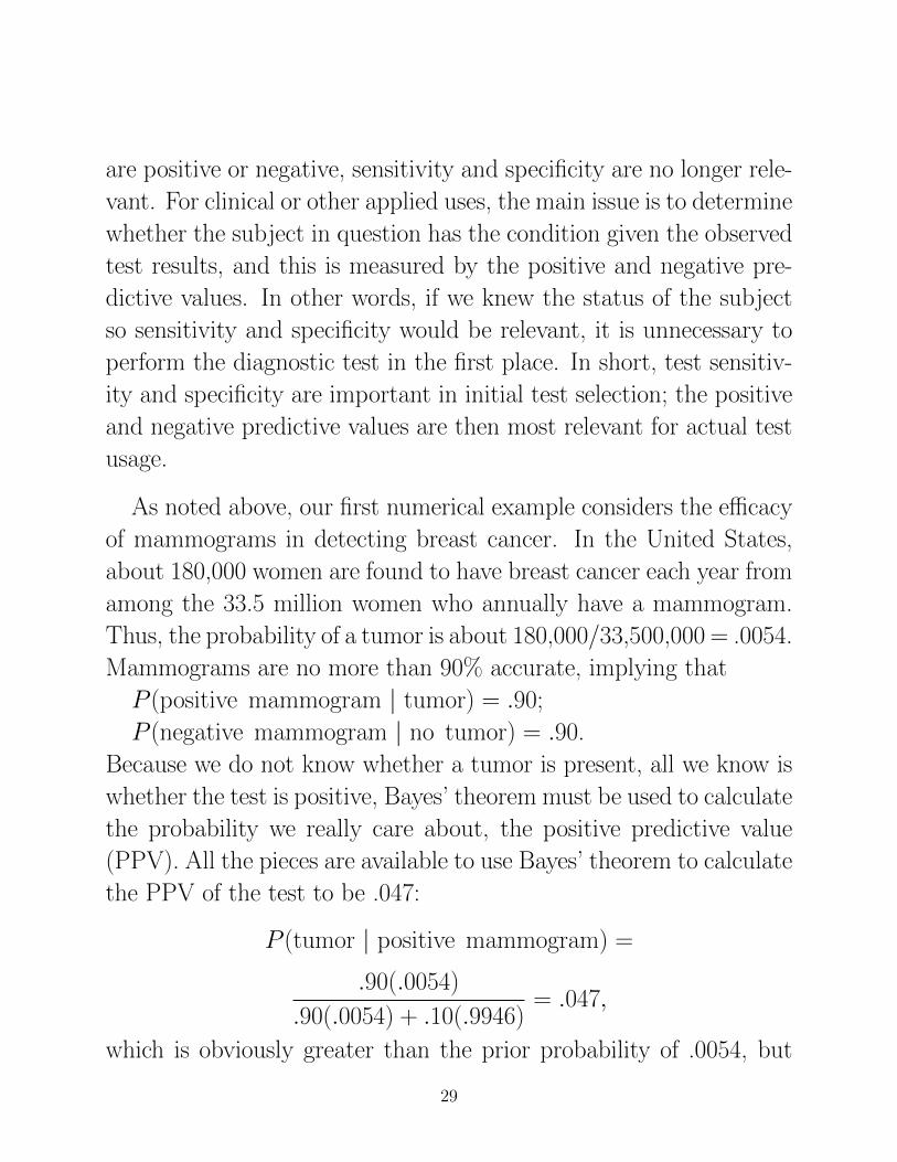
As noted above, our first numerical example considers the efficacy

of mammograms in detecting breast cancer. In the United States,

about 180,000 women are found to have breast cancer each year from

among the 33.5 million women who annually have a mammogram.

Thus, the probability of a tumor is about 180,000/33,500,000 = .0054.

Mammograms are no more than 90% accurate, implying that

P (positive mammogram | tumor) = .90;

P (negative mammogram | no tumor) = .90.

Because we do not know whether a tumor is present, all we know is

whether the test is positive, Bayes’ theorem must be used to calculate

the probability we really care about, the positive predictive value

(PPV). All the pieces are available to use Bayes’ theorem to calculate

the PPV of the test to be .047:

P (tumor | positive mammogram) =

.90(.0054)

.90(.0054) + .10(.9946)= .047,

which is obviously greater than the prior probability of .0054, but

29

still very small in magnitude; again, as in the Fecal Occult Blood

Test example, more than 95% of the positive tests that arise turn

out to be incorrect.

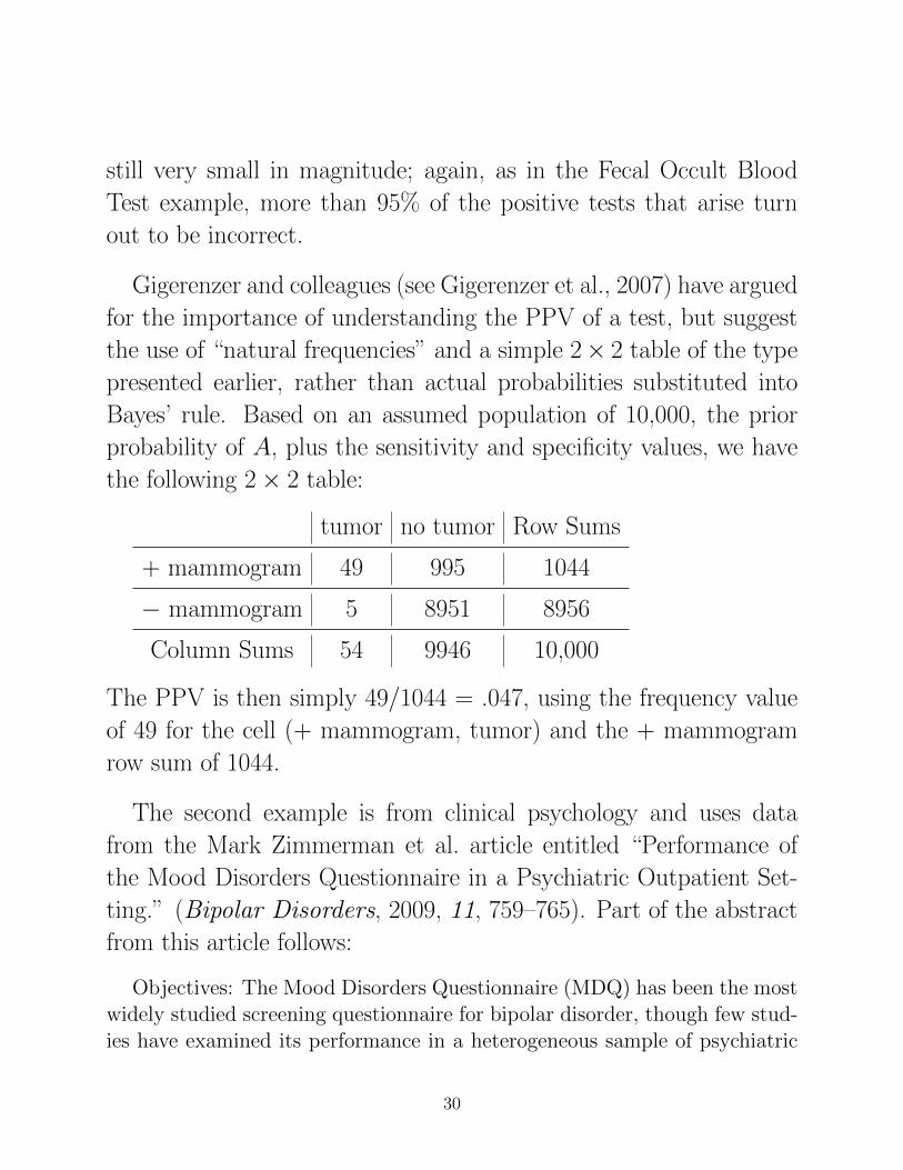
Gigerenzer and colleagues (see Gigerenzer et al., 2007) have argued

for the importance of understanding the PPV of a test, but suggest

the use of “natural frequencies” and a simple 2× 2 table of the type

presented earlier, rather than actual probabilities substituted into

Bayes’ rule. Based on an assumed population of 10,000, the prior

probability of A, plus the sensitivity and specificity values, we have

the following 2× 2 table:

tumor no tumor Row Sums

+ mammogram 49 995 1044

− mammogram 5 8951 8956

Column Sums 54 9946 10,000

The PPV is then simply 49/1044 = .047, using the frequency value

of 49 for the cell (+ mammogram, tumor) and the + mammogram

row sum of 1044.

The second example is from clinical psychology and uses data

from the Mark Zimmerman et al. article entitled “Performance of

the Mood Disorders Questionnaire in a Psychiatric Outpatient Set-

ting.” (Bipolar Disorders, 2009, 11, 759–765). Part of the abstract

from this article follows:

Objectives: The Mood Disorders Questionnaire (MDQ) has been the mostwidely studied screening questionnaire for bipolar disorder, though few stud-ies have examined its performance in a heterogeneous sample of psychiatric

30

outpatients. In the present report from the Rhode Island Methods to Im-prove Diagnostic Assessment and Services (MIDAS) project, we examinedthe operating characteristics of the MDQ in a large sample of psychiatricoutpatients presenting for treatment.

Methods: A total of 534 psychiatric outpatients were interviewed with theStructured Clinical Interview for DSM-IV and asked to complete the MDQ.Missing data on the MDQ reduced the number of patients to 480, 10.4% (n= 52) of whom were diagnosed with bipolar disorder.

Results: Based on the scoring guidelines recommended by the developersof the MDQ, the sensitivity of the scale was only 63.5% for the entire groupof bipolar patients. The specificity of the scale was 84.8%, and the positiveand negative predictive values were 33.7% and 95.0%, respectively ...

Conclusions: In a large sample of psychiatric outpatients, we found thatthe MDQ, when scored according to the developers’ recommendations, hadinadequate sensitivity as a screening measure ... These results raise questionsregarding the MDQ’s utility in routine clinical practice.

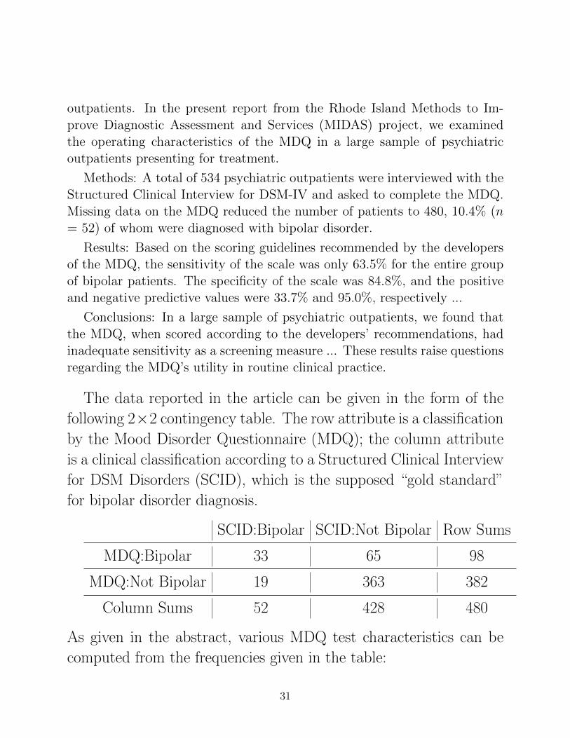
The data reported in the article can be given in the form of the

following 2×2 contingency table. The row attribute is a classification

by the Mood Disorder Questionnaire (MDQ); the column attribute

is a clinical classification according to a Structured Clinical Interview

for DSM Disorders (SCID), which is the supposed “gold standard”

for bipolar disorder diagnosis.

SCID:Bipolar SCID:Not Bipolar Row Sums

MDQ:Bipolar 33 65 98

MDQ:Not Bipolar 19 363 382

Column Sums 52 428 480

As given in the abstract, various MDQ test characteristics can be

computed from the frequencies given in the table:

31

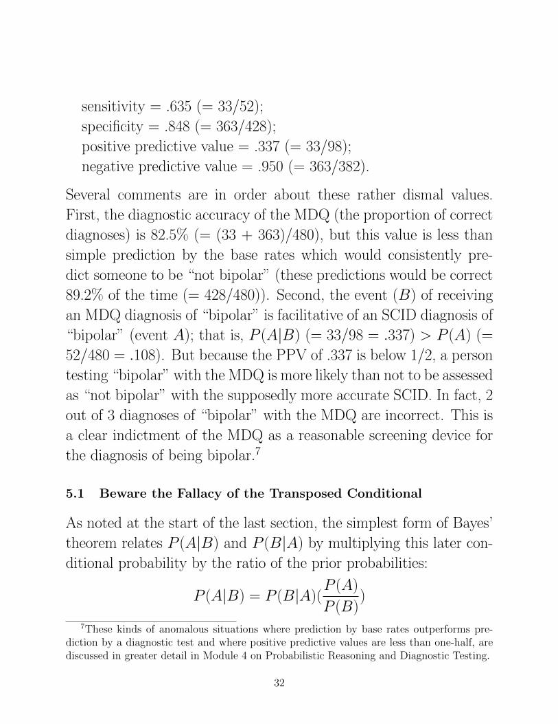
sensitivity = .635 (= 33/52);

specificity = .848 (= 363/428);

positive predictive value = .337 (= 33/98);

negative predictive value = .950 (= 363/382).

Several comments are in order about these rather dismal values.

First, the diagnostic accuracy of the MDQ (the proportion of correct

diagnoses) is 82.5% (= (33 + 363)/480), but this value is less than

simple prediction by the base rates which would consistently pre-

dict someone to be “not bipolar” (these predictions would be correct

89.2% of the time (= 428/480)). Second, the event (B) of receiving

an MDQ diagnosis of “bipolar” is facilitative of an SCID diagnosis of

“bipolar” (event A); that is, P (A|B) (= 33/98 = .337) > P (A) (=

52/480 = .108). But because the PPV of .337 is below 1/2, a person

testing “bipolar” with the MDQ is more likely than not to be assessed

as “not bipolar” with the supposedly more accurate SCID. In fact, 2

out of 3 diagnoses of “bipolar” with the MDQ are incorrect. This is

a clear indictment of the MDQ as a reasonable screening device for

the diagnosis of being bipolar.7

5.1 Beware the Fallacy of the Transposed Conditional

As noted at the start of the last section, the simplest form of Bayes’

theorem relates P (A|B) and P (B|A) by multiplying this later con-

ditional probability by the ratio of the prior probabilities:

P (A|B) = P (B|A)(P (A)

P (B))

7These kinds of anomalous situations where prediction by base rates outperforms pre-diction by a diagnostic test and where positive predictive values are less than one-half, arediscussed in greater detail in Module 4 on Probabilistic Reasoning and Diagnostic Testing.

32

Given this form of Bayes’ theorem, it is clear that for P (A|B) and

P (B|A) to be equal, the two prior probabilities, P (A) and P (B),

must first be equal. When P (A) and P (B) are not equal and then

to assert equality for P (A|B) and P (B|A), is to commit the “fallacy

of the transposed conditional,” the “inverse fallacy,” or in a legal

context, the “prosecutor’s fallacy.” We give four examples where

the fallacy of the transposed conditional can be seen at work: (1)

in the (mis-)interpretation of what a p-value signifies in statistics;

(2) returning to the Sally Clark case that opened this module, her

ultimate conviction is partly attributable to the operation of the

“prosecutor’s fallacy”; (3) in deciding when to be screened for colon

cancer by a colonoscopy rather than by a simpler and less invasive

sigmoidoscopy; (4) the confusion between test sensitivity (specificity)

and the positive (negative) predictive value.

(1) In teaching beginning statistics, it is common to define a “p-

value” somewhat as follows: assuming that a given null hypothesis,

Ho, is true, the p-value is the probability of seeing a result as or more

extreme than what was actually observed. It is not the probability

that the null hypothesis is true given what was actually observed.

The latter is an example of the fallacy of the transposed conditional.

Explicitly, the probability of seeing a particular data result condi-

tional on the null hypothesis being true, P (data | Ho), is confused

with P (Ho | data), the probability that the null hypothesis is true

given that a particular data result has occurred.

(2) For our second example, we return to the Sally Clark conviction

where the invalidly constructed probability of 1 in 73 million was

used to successfully argue for Sally Clark’s guilt. Let A be the event

33

of innocence and B the event of two “cot deaths” within the same

family. The invalid probability of 1 in 73 million was considered

to be for P (B|A); a simple equating with P (A|B), the probability

of innocence given the two cot deaths, led directly to Sally Clark’s

conviction.8

We continue with the Royal Statistical Society news release:

Aside from its invalidity, figures such as the 1 in 73 million are very eas-ily misinterpreted. Some press reports at the time stated that this was thechance that the deaths of Sally Clark’s two children were accidental. This(mis-)interpretation is a serious error of logic known as the Prosecutor’s Fal-lacy.

The Court of Appeal has recognised these dangers (R v. Deen 1993, R v.Doheny/Adams 1996) in connection with probabilities used for DNA profileevidence, and has put in place clear guidelines for the presentation of suchevidence. The dangers extend more widely, and there is a real possibilitythat without proper guidance, and well-informed presentation, frequency es-timates presented in court could be misinterpreted by the jury in ways thatare very prejudicial to defendants.

Society does not tolerate doctors making serious clinical errors becauseit is widely understood that such errors could mean the difference betweenlife and death. The case of R v. Sally Clark is one example of a medicalexpert witness making a serious statistical error, one which may have had aprofound effect on the outcome of the case.

Although many scientists have some familiarity with statistical methods,statistics remains a specialised area. The Society urges the Courts to ensurethat statistical evidence is presented only by appropriately qualified statisticalexperts, as would be the case for any other form of expert evidence.

8The exact same circumstances can occur in the (mis)use of DNA evidence. Here, theevent B is the existence of a “match” between a suspect’s DNA and what was found, say, atthe crime scene; the event A is again one of innocence. The value for P (B|A) is the proba-bility of a DNA match given that the person is innocent. Commission of the “prosecutor’sfallacy” would reverse the conditioning and say that this latter probability is actually forP (A|B), the probability of innocence given that a match occurs.

34

(3) The third example is inspired by Edward Beltrami’s book,

Mathematical Models for Society and Biology (Academic Press;

2013), and in particular, its Chapter 5 on “A Bayesian Take on Col-

orectal Screening ...”9 We begin with several selective quotations

from an article in the New York Times by Denise Grady (July 20,

2000), “More Extensive Test Needed For Colon Cancer, Studies Say”:

The test most commonly recommended to screen healthy adults for col-orectal cancer misses too many precancerous growths and should be replacedby a more extensive procedure that examines the entire colon, doctors arereporting today.

...The more common test, sigmoidoscopy, reaches only about two feet into

the colon and is generally used to screen people 50 and older with an averagerisk of colon cancer. The more thorough procedure, colonoscopy, probes thefull length of the colon, 4 to 5 feet, and is usually reserved for people with ahigher risk, like those with blood in their stool, a history of intestinal polypsor a family history of colon cancer.

...Sigmoidoscopy, which is cheaper and easier to perform, has been used for

screening on the optimistic theory that if no abnormalities were seen in thelower colon, none were likely to be found higher up.

But that theory is contradicted by two studies being published today inThe New England Journal of Medicine, which included a total of more than5,000 healthy people screened by colonoscopy. One study, which involvedmore than 3,000 patients, is the largest study to date of the procedure. Bothstudies show that it is not safe to assume that the upper colon is healthyjust because the lower third looks normal. The studies found that half thepatients who had precancerous lesions in the upper colon had nothing abnor-

9As readers, you may wonder where we have our minds, given that an earlier numericalexample used a Fecal Occult Blood Test to check for Colorectal cancer, but trust us, this is avery informative example of how the fallacy of the transposed conditional plays an importantrole in fostering misunderstanding within “evidence-based-medicine” and how the media thenperpetuates the interpretative error.

35

mal lower down. If those patients had had only sigmoidoscopy, they wouldhave mistakenly been given a clean bill of health and left with dangerous,undetected growths high in the colon.

Based on the two studies mentioned by Denise Grady and the

analyses done by Beltrami, we have approximately the following

conditional probabilities involving the two events U : there are ad-

vanced upper colon lesions, and L: there are no lower colon polyps:

P (U |L) ≈ .02 and P (L|U) ≈ .50. A doctor wishing to convince

a patient to do the full colonoscopy might well quote the second

statistic, P (L|U), and say “50% of all upper colon cancerous polyps

would be missed if only the sigmoidoscopy were done.” Although

this statement is true, it might not be as convincing to undergo

the much more invasive colonoscopy compared to a sigmoidoscopy if

the first statistic, P (U |L), were then quoted: “there is a very small

probability of 2% of the upper colon showing cancerous lesions if the

sigmoidoscopy shows no lower colon polyps.” Confusing the 2% in

this last statement with the larger 50% amounts to the commission

of the transposition fallacy.

(4) The last example deals with the generic diagnostic testing con-

text where B is the event of testing “positive” and A is the event

that the person really is “positive.” Equating sensitivity and the

positive predictive value requires P (A|B) to be equal to P (B|A); or

in words, the probability of having “it” given that the test is positive

must be the same as the test being positive if the person really does

have it. As our example on breast cancer screening illustrates, if the

base rate for having cancer is small (as it is here: P (A) = .0054),

and differs from the probability of a positive test (as it does here:

P (B) = .90(.0054) + .10(.9946) = .1044), the positive predictive

36

value can be very disappointing (P (A|B) = .047; so there are about

95% false positives), and nowhere near the assumed test sensitivity

(P (B|A) = .90).

6 Probability of Causation

In mass (toxic) tort cases (such as for asbestos, breast implants, and

Agent Orange) there is a need to establish, in a legally acceptable

fashion, some notion of causation. First, there is a concept of gen-

eral causation concerned with whether an agent can increase the

incidence of disease in a group; because of individual variation, a

toxic agent will not generally cause disease in every exposed indi-

vidual. Specific causation deals with an individual’s disease being

attributable to exposure from an agent.

The establishment of general causation (and a necessary require-

ment for establishing specific causation) typically relies on a cohort

study. This is a method of epidemiologic study where groups of indi-

viduals are identified who have been or in the future may be differen-

tially exposed to agent(s) hypothesized to influence the probability

of occurrence of a disease or other outcome. The groups are observed

to assess whether the exposed group is more likely to develop disease.

One common way to organize data from a cohort study is through

a simple 2×2 contingency table, similar in form to those seen earlier

in this introductory discussion:

Disease No Disease Row Sums

Exposed N11 N12 N1+

Not Exposed N21 N22 N2+

37

Here, N11, N12, N21, and N22 are the cell frequencies; N1+ and N2+

are the row frequencies. Conceptually, these data are considered

generated from two (statistically independent) binomial distributions

for the “Exposed” and “Not Exposed” conditions. If we let pE and

pNE denote the two underlying probabilities of getting the disease

for particular cases within the conditions, respectively, the ratio pEpNE

is referred to as the relative risk (RR), and may be estimated with

the data as follows:

estimated relative risk = RR = pEpNE

= N11/N1+N21/N2+

.

A measure commonly referred to in tort litigations is attributable

risk (AR), defined as

AR = pE − pNEpE

, and estimated by

AR = pE − pNEpE

= 1− 1

RR.

Attributable risk, also known as the “attributable proportion of risk”

or the “etiologic fraction,” represents the amount of disease among

exposed individuals assignable to the exposure. It measures the max-

imum proportion of the disease attributable to exposure from an

agent, and consequently, the maximum proportion of disease that

could be potentially prevented by blocking the exposure’s effect or

eliminating the exposure itself. If the association is causal, AR is the

proportion of disease in an exposed population that might be caused

by the agent, and therefore, that might be prevented by eliminating

exposure to the agent.

The common legal standard used to argue for both specific and

general causation is an RR of 2.0, or an AR of 50%. At this level,

it is “as likely as not” that exposure “caused” the disease (or “as

likely to be true as not,” or from English law, “the balance of the

38

probabilities”). Obviously, one can never be absolutely certain that

a particular agent was “the” cause of a disease in any particular

individual, but to allow an idea of “probabilistic causation” or “at-

tributable risk” to enter into legal arguments provides a justifiable

basis for compensation. It has now become routine to do this in the

courts.

Besides toxic tort cases, genetics is an area where the idea of at-

tributable risk is continually discussed in informed media outlets such

as the New York Times. The “penetrance” of a particular genetic

anomaly or mutation was briefly explained earlier in the context of

Angelina Jolie’s decision to undergo a preventive mastectomy. But

there now seems to be a stream of genetic studies reported on reg-

ularly where an informed understanding of attributable and relative

risk would be of benefit for our own personal medical decision mak-

ing. To give one such example, again in the context of genetics and

contracting breast cancer, we have the recent article in the New York

Times by Nicholas Bakalar (August 6, 2014), entitled “Study Shows

Third Gene as Indicator for Breast Cancer.” Several paragraphs of

this piece are given below that emphasize attributable and relative

risk in some detail:

Mutations in a gene called PALB2 raise the risk of breast cancer in womenby almost as much as mutations in BRCA1 and BRCA2, the infamous genesimplicated in most inherited cases of the disease, a team of researchers re-ported Wednesday.

...Over all, the researchers found, a PALB2 mutation carrier had a 35 percent

chance of developing cancer by age 70. By comparison, women with BRCA1mutations have a 50 percent to 70 percent chance of developing breast cancerby that age, and those with BRCA2 have a 40 percent to 60 percent chance.

39

The lifetime risk for breast cancer in the general population is about 12percent.

The breast cancer risk for women younger than 40 with PALB2 mutationwas eight to nine times as high as that of the general population. The riskwas six to eight times as high among women 40 to 60 with these mutations,and five times as high among women older than 60.

6.1 The Energy Employees Occupational Illness CompensationProgram (EEOICP)

David Michaels is the current Assistant Secretary of Labor for the Oc-

cupational Safety and Health Administration (OSHA); he was nom-

inated by President Obama and unanimously confirmed by the U.S.

Senate in 2009 – quite a feat in an era of Congressional gridlock.

During the Clinton administration, Michaels served as the United

States Department of Energy’s Assistant Secretary for Environment,

Safety, and Health (1998–2001), where he developed the initiative

to compensate workers in the nuclear weapons industry who devel-

oped cancer or lung disease as a consequence of exposure to radi-

ation, beryllium, and other toxic hazards. The initiative resulted

in the program that entitles this section, and which has provided

some ten billion dollars in benefits since its inception in 2001. David

Michaels, an epidemiologist on leave from George Washington Uni-

versity School of Public Health and Health Services, is also the author

of the well-received book, Doubt is Their Product: How industry’s

assault on science threatens your health (2008; Oxford).

The EEOICP was signed into law on December 7, 2000 by Presi-

dent Clinton, along with Executive Order 13179 reproduced below:

Since World War II, hundreds of thousands of men and women have served

40

their Nation in building its nuclear defense. In the course of their work, theyovercame previously unimagined scientific and technical challenges. Thou-sands of these courageous Americans, however, paid a high price for theirservice, developing disabling or fatal illnesses as a result of exposure to beryl-lium, ionizing radiation, and other hazards unique to nuclear weapons produc-tion and testing. Too often, these workers were neither adequately protectedfrom, nor informed of, the occupational hazards to which they were exposed.

Existing workers’ compensation programs have failed to provide for theneeds of these workers and their families. Federal workers’ compensationprograms have generally not included these workers. Further, because oflong latency periods, the uniqueness of the hazards to which they were ex-posed, and inadequate exposure data, many of these individuals have beenunable to obtain State workers’ compensation benefits. This problem hasbeen exacerbated by the past policy of the Department of Energy (DOE)and its predecessors of encouraging and assisting DOE contractors in oppos-ing the claims of workers who sought those benefits. This policy has recentlybeen reversed.

While the Nation can never fully repay these workers or their families, theydeserve recognition and compensation for their sacrifices. Since the Adminis-tration’s historic announcement in July 1999 that it intended to compensateDOE nuclear weapons workers who suffered occupational illnesses as a resultof exposure to the unique hazards in building the Nation’s nuclear defense, ithas been the policy of this Administration to support fair and timely compen-sation for these workers and their survivors. The Federal Government shouldprovide necessary information and otherwise help employees of the DOE orits contractors determine if their illnesses are associated with conditions oftheir nuclear weapons-related work; it should provide workers and their sur-vivors with all pertinent and available information necessary for evaluatingand processing claims; and it should ensure that this program minimizes theadministrative burden on workers and their survivors, and respects their dig-nity and privacy. This order sets out agency responsibilities to accomplishthese goals, building on the Administration’s articulated principles and theframework set forth in the Energy Employees Occupational Illness Compen-sation Program Act of 2000. The Departments of Labor, Health and Human

41

Services, and Energy shall be responsible for developing and implementingactions under the Act to compensate these workers and their families in amanner that is compassionate, fair, and timely. Other Federal agencies, asappropriate, shall assist in this effort.

The EEOICP is one of the most successful and well-administered

Federal compensation programs. It has its own non-profit advocacy

group called “Cold War Patriots” (submotto: We did our part to

keep America Free!); the web site for this organization is:

www.coldwarpatriots.org

This advocacy group provides informational meetings and help for

those who might be eligible under the program. Below is part of an ad

that appeared in the New Mexican (Santa Fe, New Mexico; June,

2014) announcing informational meetings in Penasco, Los Alamos,

and Espanola:

Attention Former LANL (Los Alamos National Lab), Sandia Labs,

and Uranium Workers:

— Join us for an important town hall meeting

— Learn if you qualify for benefits up to $400,000 through the

Energy Employees Occupational Illness Compensation Program Act

(EEOICPA)

— Learn about no-cost medical benefit options

— Learn how to apply for consequential medical conditions and

for impairment re-evaluation for approved conditions

The EEOICP represents an implementation of the “as likely as

not standard” for attributing possible causation (and compensation),

and has gone to great technical levels (and which should keep many

42

biostatisticians gainfully employed for years to come). What fol-

lows in an appendix is an extensive excerpt from the Federal Regis-

ter concerning the Department of Health and Human Services and

its Guidelines for Determining the Probability of Causation and

Methods for Radiation Dose Reconstruction Under the [Energy]

Employees Occupational Illness Compensation Program Act of

2000. This material should give a good sense of how the model-

ing principles of probability and statistics are leading to ethically

defensible compensation models; here, the models used are for all

those exposed to ionizing radiation through an involvement with the

United States’ nuclear weapons industry.10

10Several points need emphasize about this Federal Register excerpt: (1) the calculationof a “probability of causation” is much more sophisticated (and fine-grained) than one basedon a simple aggregate 2×2 contingency table where attributable risk (AR) is just calculatedfrom the explicit cell frequencies. Statistical models (of what are commonly referred to as thegeneralized linear model variety) are being used to estimate the AR tailored to an individual’sspecific circumstances—type of cancer, type of exposure, other individual characteristics;(2) all the models are now implemented (interactively through a graphical user interface)within the Interactive RadioEpidemiological Program (IREP), making obsolete the verycumbersome charts and tables previously used; also, IREP allows a continual updating tothe model estimation process when new data become available; (3) it is not just a pointestimate for the probability of causation that is used to determine compensation, but ratherthe upper limit for a 99% confidence interval; this obviously gives a great “benefit of thedoubt” to an individual seeking compensation for a presumably radiation-induced disease;(4) as another “benefit of the doubt” calculation, if there are two or more primary cancers,the probability of causation reported will be the probability that at least one of the cancerswas caused by the radiation. Generally, this will result in a larger estimate for the probabilityof causation, and thus to a greater likelihood of compensation; (5) when cancers are identifiedfrom secondary sites and the primary site is unknown, the final assignment of the primarycancer site will be the one resulting in the highest estimate for the probability of causation.

43

7 The Interpretation of Probability and Risk

The Association for Psychological Science publishes a series of timely

monographs on Psychological Science in the Public Interest. One

recent issue was from Gerd Gigerenzer and colleagues, entitled “Help-

ing Doctors and Patients Make Sense of Health Statistics” (Gigeren-

zer et al., 2007). It discusses aspects of statistical literacy as it con-

cerns health, both our own individually as well as societal health

policy more generally. Some parts of being statistically literate may

be fairly obvious; we know that just making up data, or suppressing

information even of supposed outliers without comment, is unethical.

The topics touched upon by Gigerenzer et al. (2007), however, are

more subtle. If an overall admonition is needed, it is that context is

always important, and the way data and information are presented

is absolutely crucial to an ability to reason appropriately and act ac-

cordingly. We review several of the major issues raised by Gigerenzer

et al. in the discussion to follow.

We begin with a quotation from Rudy Guiliani from a New Hamp-

shire radio advertisement that aired on October 29, 2007, during his

run for the Republican presidential nomination:

I had prostate cancer, five, six years ago. My chances of surviving prostatecancer and thank God I was cured of it—in the United States, 82 percent.My chances of surviving prostate cancer in England, only 44 percent undersocialized medicine.

Not only did Guiliani not receive the Republican presidential nom-

ination, he was just plain wrong on survival chances for prostate

cancer. The problem is a confusion between survival and mortality

44

rates. Basically, higher survival rates with cancer screening do not

imply longer life.

To give a more detailed explanation, we define a five-year survival

rate and an annual mortality rate:

five-year survival rate = (number of diagnosed patients alive after

five years)/(number of diagnosed patients);

annual mortality rate = (number of people who die from a disease

over one year)/(number in the group).

The inflation of a five-year survival rate is caused by a lead-time

bias, where the time of diagnosis is advanced (through screening)

even if the time of death is not changed. Moreover, such screening,

particularly for cancers such as prostate, leads to an overdiagno-

sis bias, the detection of a pseudodisease that will never progress

to cause symptoms in a patient’s lifetime. Besides inflating five-year

survival statistics over mortality rates, overdiagnosis leads more sinis-

terly to overtreatment that does more harm than good (for example,

incontinence, impotence, and other health-related problems).

Screening does not “prevent cancer,” and early detection does not

prevent the risk of getting cancer. One can only hope that cancer is

caught, either by screening or other symptoms, at an early enough

stage to help. It is also relevant to remember that more invasive

treatments are not automatically more effective. A recent and infor-

mative summary of the dismal state and circumstances surrounding

cancer screening generally, appeared in the New York Times as a

“page one and above the fold” article by Natasha Singer (July 16,

2009), “In Push for Cancer Screening, Limited Benefits.”

45

A major area of concern in the clarity of reporting health statistics

is in how the data are framed as relative risk reduction or as absolute

risk reduction, with the former usually seeming much more important

than the latter. We give examples that present the same information:

Relative risk reduction: If you have this test every two years, your

chance of dying from the disease will be reduced by about one third

over the next ten years.

Absolute risk reduction : If you have this test every two years, your

chance of dying from the disease will be reduced from 3 in 1000 to 2

in 1000, over the next ten years.11

A useful variant on absolute risk reduction is given by its reciprocal,

the number needed to treat (NNT); if 1000 people have this test

every two years, one person will be saved from dying from the disease

every ten years. (Numerically, the NNT is just the reciprocal of the11In informed media outlets such as the New York Times, the distinction between relative

and absolute risk reduction is generally highlighted whenever there is also a downside to themedical procedure being reported. An example of this caution is present in the article by TaraParker-Pope (August 6, 2014), entitled “Prostate Cancer Screening Still Not Recommendedfor All.” The article gives a lifetime risk of dying of prostate cancer of 3 percent and adrop to 2.4 percent under a PSA testing regime. Although the absolute risk reduction of.6 percent does represent a 21 percent lower relative risk of dying, it is highly questionablewhether this drop is worth the over-diagnosis and over-treatment that it requires. A fewparagraphs from the article follow:

A major European study has shown that blood test screening for prostate cancer saveslives, but doubts remain about whether the benefit is large enough to offset the harms causedby unnecessary biopsies and treatments that can render men incontinent and impotent.

The study, published Wednesday in The Lancet, found that midlife screening with theprostate-specific antigen, or PSA, screening test lowers a man’s risk of dying of the diseaseby 21 percent. The relative benefit sounds sizable, but it is not particularly meaningful tothe average middle-age man, whose risk of dying of prostate cancer without screening isabout 3 percent. Based on the benefit shown in the study, routine PSA testing would lowerhis lifetime cancer risk to about 2.4 percent.

46

absolute risk reduction, or in this case, 1/(.003 − .002) = 1/.001 =

1000.)12

Because bigger numbers garner better headlines and more media

attention, it is expected that relative rather than absolute risks are

the norm. It is especially disconcerting, however, to have poten-

tial benefits (of drugs, screening, treatments, and the like) given in

relative terms, but harm in absolute terms that is typically much

smaller numerically. The latter has been referred to as “mismatched

framing” by Gigerenzer and colleagues.

The issues involved in presenting two probabilities or proportions

either as an absolute difference or relatively as a ratio reappears

continually when there is a need to assess and report magnitudes.

For example, in the Fecal Occult Blood Test illustration, the absolute

difference between P (+CC | + FOBT ) and P (+CC) was a small

value of +.045 (but still would be one way of stating the degree of

facilitation of +FOBT on +CC). As a ratio, however, with respect

to the prior probability of .003 for P (+CC), this absolute difference

does represent a fifteen-fold change. So, a relative measure again

appears much more impressive than an absolute difference. All of

this, by the way, is in the context of a very large false positive rate

of over 95%. The exact same story is told in the illustration for

breast cancer screening with mammography: we have small absolute

differences, large relative ratios, and dismal performances as to the12In addition to the use of relative and absolute risk, or the number needed to treat, a

fourth way of presenting benefit would be as an increase in life expectancy. For example,one might say that women who participate in screening from the ages of 50 to 69 increasetheir life expectancy by an average of 12 days. This is misleading in terms of a benefit toany one particular individual; it is much more of an all-or-nothing situation, like a lottery.Nobody who plays a lottery gains the expected payout; you either win it all or not.

47

occurrence of false positives.

An ethical presentation of information avoids nontransparent fram-

ing of information, whether intentional or unintentional. Intentional

efforts to manipulate or persuade people are particularly destruc-

tive, and unethical by definition. As Tversky and Kahneman have

noted many times (for example, 1981), framing effects and context

have major influences on a person’s decision processes. Whenever

possible, give measures that have operational meanings with respect

to the sample at hand (for example, the Goodman–Kruskal gamma,

the median or the mode, the interquartile range) and avoid measures

that do not, such as the odds ratio (discussed in greater detail in a

subsection to follow).

7.1 Where Do the Numbers Come From that Might Be Referredto as Probabilities and What Do They Signify

The introductory section of this module introduced the notion of

probability as some number between zero and one that could be

attached to an event, say A. The numbers so assigned were as-

sumed implicitly to satisfy the usual axioms of probability theory,

particularly the additive property for mutually exclusive events. The

presentation here will be brief and necessarily basic, and follows a

few simple distinctions that might be made in a beginning statistics

class. For a much more thorough introduction to the topic of where

probabilities come from that touches on a several hundred-year his-

tory, the reader is referred to the on-line Stanford Encyclopedia of

Philosophy and the article “Interpretations of Probability.”13

13However it is done, in assigning numbers to the occurrence of an event or to the truthof some statement, it may at times be of value to separate out the actual numerical estimate

48

A distinction can be made between two broad categories of meth-

ods for assigning probabilities: objective and subjective. An objec-

tive method is based on some point-at-able that might, for example,

be a randomly controlled physical system or a database containing a

variety of objects and attributes that could be queried to estimate a

set of desired relative frequencies (or probabilities under an implicit

urn model). A subjective method for assigning probabilities would

typically be subject-specific, and based on some collection of pre-

sented evidence or result from aggregating the assessments of others.

We begin with objective assignment methods.

As noted in greater detail in Module 5 on Probabilistic Reasoning

in the Service of Gambling, the foundations of a modern theory of

probability were laid down by Blaise Pascal and Pierre de Fermat in

the early 17th century in response to a request from the Chevalier de

Mere. This has become known as the “classical definition” of prob-

ability, and rests on the idea that some random process produces

from one’s confidence in it. For example, in throwing two dice a probability of 6/36 might beassigned for getting a seven and with complete confidence in that assignment. A weatherman,however, may be very confident about a forecast of 30 percent rain for tomorrow but maybe very uncertain when that same forecast of 30 percent rain is made for a week from now.In considering the range of reasonable forecasts for tomorrow, there may be some smalluncertainty around the 30% estimate; a week from now, however, and even though the sameestimate of 30% might be made, there is a much larger range of uncertainty around thatsame value – or as the old adage goes: there is many a slip ‘twixt the cup and the lip.

At times there may be some equivocation between what is a probability estimate andwhat is one’s confidence in that estimate. For example, an eyewitness who picks a particularsubject out of a line-up has, in effect, assigned a probability of 1.0 to the event that the personis the “perp“; if pressed, additional phrases such as “yup, he’s the one” or “I could see prettygood in the moonlight” express various levels of confidence in that initial assessment. In theevaluation discussed later as to whether Osama bin Laden would be at the compound inPakistan when the Navy SEALs arrived, the values given in this particular vignette mayreflect more confidence than (degree-of-belief) probability for the statement “bin Laden isat Abad Abad all the time.”

49

outcomes that can be considered equally-likely. We give a quotation

from Pierre-Simon Laplace (A Philosophical Essay on Probabili-

ties, 1814):

The theory of chance consists in reducing all the events of the same kindto a certain number of cases equally possible, that is to say, to such as we maybe equally undecided about in regard to their existence, and in determiningthe number of cases favorable to the event whose probability is sought. Theratio of this number to that of all the cases possible is the measure of thisprobability, which is thus simply a fraction whose numerator is the number offavorable cases and whose denominator is the number of all the cases possible.

As a simple example involving the random process of tossing two

dice, the 36 pairs of integers from 1 to 6 could be considered equally

likely. Out of the 36 pairs, 6 have the sum of spots equal to 7 ((6,1),

(1,6), (2,5), (5,2), (4,3), (3,4)); thus, the probability of the event of

rolling a 7 is 6/36.

A second objective method of assigning (approximate) probabili-

ties is through observed relative frequencies. Here, there are n trials

in which the event, say, A, could have occurred, and on nA of these,

event A did occur. Thus, P (A) ≈ nA/n, which is assumed to con-

verge to the true probability as n goes to infinity (that is, “in the

long run”). The type of repeated sampling using an urn model and

obtaining the relative frequencies for the events of interest would be

another example of this type of assignment.

A third form of objective probability assignment might be called

the “database strategy.” For example, suppose we have a multi-way

contingency table that cross-classifies women according to various

personal attributes, and as to whether they have the BRAC1 muta-

50

tion and have contracted breast cancer (over their lifetimes). Enter-

ing the multi-way table with the personal attributes of Angelina Jolie

and her positive status on the BRAC1 mutation, the proportion of

women with these same characteristics that contracted breast can-

cer would be a probability estimate for her contracting breast cancer

(that is, the value of .87 given in an earlier section).

The NPR News program, All Things Considered, ran a series

of five programs on Risk and Reason in the Summer of 2014 that

all dealt with probability in some way. One discussed weather fore-

casting: “Pop Quiz: 20 Percent Chance of Rain. Do You Need An

Umbrella?” The issue discussed was how people generally interpreted

the value of 20 percent. The best answer was to consider a database

assignment: “it will rain on 20 percent of the days like tomorrow.”

Or, from a followup clarification (July 23, 2014):

Many listeners and readers felt a concise explanation of “a 20 percentchance of rain” was missing from this story about weather forecasts andprobability, so we followed up with two meteorologists.

Will it rain or not? How you interpret the forecast could mean the differ-ence between getting soaked or staying safe.

From meteorologist Eli Jacks, of the National Oceanic and AtmosphericAdministration’s National Weather Service:

“There’s a 20 percent chance that at least one-hundredth of an inch ofrain – and we call that measurable amounts of rain – will fall at any specificpoint in a forecast area.”

And from Jason Samenow, chief meteorologist with The Washington Post ’sCapital Weather Gang:

“It simply means for any locations for which the 20 percent chance of rainapplies, measurable rain (more than a trace) would be expected to fall in twoof every 10 weather situations like it.”

51

The last form of objective probability assignment might be called

“algorithmic” and would be represented by Nate Silver’s FiveThir-

tyEight Blog that nicely predicted the outcome of the 2012 Presi-

dential Election. The method used by Nate Silver involves aggregat-

ing information about some subject (for example, impending Senate

races) across available polls that are weighted in various ways accord-

ing to assumed biases – a nascent Bayesian approach some might say.

Such aggregated probability estimates are another “objective” means

for assigning probabilities that appears to work remarkably well.14

Now that Nate Silver has moved on to ESPN, the New York

Times has a new statistical Blog called The Upshot, edited by David

Leonhardt. As an example of the type of probability assessments

they now give, we extract a first few paragraphs from an article

about the 2014 midterm elections by Amanda Cox and Josh Katz,

“Republicans’ Senate Chances Rise Slightly to 60 Percent” (July 27,

2014):

For the last month, we’ve been adding one or two polls a day to TheUpshot ’s Senate forecasting model. Today, we update all 36 races, based onestimates from a YouGov online panel that covers every congressional andgovernor’s race across the country.

The panel, asked for its preferences in collaboration with CBS and TheNew York Times, is unusual in its scope: It comprises more than 66,000people living in states with a Senate race this year. YouGov, a polling firm,also conducted online interviews with roughly half of the panelists in previousyears, allowing it to know how they voted in the past.

With the addition of the YouGov estimates to our model, the overall out-look for the Senate remains roughly the same. The Republicans appear to

14Nate Silver’s success has raised the self-esteem of all statisticians. The Associated Pressstates that “Nate Silver had made statistics sexy again”; Bloomberg Businessweek commentsthat “Nate Silver-led statistics men crush pundits in election.”

52

have a slight advantage, with the most likely outcome being a Republicangain of six seats, the minimum they need to finish with a 51-to-49-seat ma-jority. But we, like many other forecasters, would not be surprised by a gainof anywhere from four to eight seats.

Summing up the possible outcomes, our model gives the Republicans a 60percent chance of taking control, up from 54 percent on April 1.

Polls are only one part of the model. (And we adjust polls from partisanfirms according to our best estimates of how Republican- or Democratic-leaning the pollster has been this cycle.) The model also includes the can-didates’ political experience, fund-raising, a state’s past election results andnational polling.

The relative weight of these factors depends on the number and the qualityof the polls in each state, as well as how useful each factor was in predictingpast Senate elections. Currently, polls make up about 80 percent of theforecast in the most competitive races.

A subjective assignment of probability typically takes the form of

an individual, or a group of individuals such as a jury or committee,

receiving information (or hearing evidence) about the potential oc-

currence of some event or the truth of some statement. This latter

assessment might be given in terms of explicit numbers that signify

probability, or alternatively, in words that might suggest a (numeri-

cal) range of possibilities; for example, an assessment of a “prepon-

derance of the evidence” suggests some numerical value greater than

one-half. A particularly good example of the issue of using words

versus numbers to refer to subjective (or “evidentiary”) probabilities

was in the second program in the NPR series on Risk and Reason

that aired on July 23, 2014, entitled “In Facing National Security

Dilemmas, CIA Puts Probabilities Into Words.” This program dealt

with the circumstantial evidence of Osama bin Laden’s whereabouts,

how the evidence was assessed by individuals in the CIA, and even-

53

tually on the assessment of President Obama before he made the

decision for the Navy SEALs to invade the compound in Pakistan.

We give a few paragraphs from the show’s transcript (with Host,

Robert Siegel) that concern using numbers and/or words to indicate

the likeliness of bin Laden being in the Abad Abad compound:15

...KENNETH POLLACK: There was a real injunction that no one should

ever use numbers to explain probability.SIEGEL: That’s Kenneth Pollack who used to be a military analyst at the

CIA, where he now teaches intelligence analysis. Pollack says CIA analystsare told if you are asked what the chances of something happening, use words.

POLLACK: Almost certainly or highly likely or likely or very unlikely.SIEGEL: What’s the problem with numbers?POLLACK: Assigning numerical probability suggests a much greater de-

gree of certainty than you ever want to convey to a policymaker. What weare doing is inherently difficult. Some might even say it’s impossible. We’retrying to project the future. And, you know, saying to someone that there’sa 67 percent chance that this is going to happen, that sounds really precise.And that makes it seem like we really know what’s going to happen. Andthe truth is that we really don’t.

SIEGEL: So Ken Pollack was surprised by the accounts of one especiallyhigh-profile event, in which CIA analysts and others in the intelligence agen-cies used numbers, very specific numbers, to express probabilities. Let’s goback to May 1, 2011.

...PRESIDENT BARACK OBAMA: Good evening. Tonight, I can report to

the American people and to the world that the United States has conducted

15We need to remember that any number attached to the event that bin Laden is atthe Abad Abad compound is a statement about “degree-of-belief.” It does not refer to anyrepeatable event. The latter would require something like the following fanciful situation: binLaden comes and goes from the compound more or less randomly each day; the probabilitythat bin Laden happens to be at the compound when the Navy SEALs show up is based onsome estimate of time that he is at home.

54

an operation that killed Osama bin Laden, the leader of al-Qaida.SIEGEL: According to writers who investigated the decision to send Navy

SEALs to the compound in Abad Abad, Pakistan, the estimates of certaintythat bin Laden was the man they’d spotted in the compound covered a range.Both Peter Bergen and Mark Bowden wrote separately that the lead analystat the CIA put his confidence level at 90 percent or 95 percent. The deputydirector of the CIA was at 60 percent. Other analysts, they say, settled ona much lower number – 40 percent. A week after the raid, President Obamawent on “60 Minutes” and acknowledged that it’d been a tough decision,because the evidence was circumstantial.

(SOUNDBITE OF TV SHOW, “60 MINUTES”)OBAMA: At the end of the day, this was still a 55-45 situation. I mean,

we could not say definitively that bin Laden was there.SIEGEL: Other accounts have Obama concluding it was basically 50-50 –

a coin flip. Reading these accounts, Jeff Friedman wondered about how theintelligence analysts had presented their views and whether they could’vedone it better. Friedman researches national security decision-making as apostdoctoral fellow at Dartmouth. He’s the co-author of a paper examiningthe decision to stage the raid on Abad Abad. And he says this – people’sbeliefs about how probable something is are subjective and how much wetrust those people is also subjective. But Jeff Friedman argues you can stillpicture the subjective judgments effectively, especially if you remember wherepeople making those judgments are coming from, as in the bin Laden case.

JEFF FRIEDMAN: The low estimate of 30 or 40 percent likelihood thatbin Laden was at Abad Abad was issued by a CIA red team. And thered team, which is a common institutional practice, is to be skeptical onpurpose, right? They were meant to poke holes in the intelligence. So they,of course, came out the lowest estimate – 30 or 40 percent. The deputydirector of Intelligence, Michael Morell, says that he assessed that there wasa 60 percent chance that bin Laden would be at Abad Abad. And he tellsPresident Obama explicitly that he’s lowballing that assessment a bit becausehe remembers this assessment of Iraq’s weapons of mass destruction. And heknows how easy it is to sort of connect these dots and to be overoptimisticin Intelligence. What does President Obama do, in the end? He says it’s a

55

coin flip. We’re going with 50-50. So he ends up implicitly giving the mostweight to the estimates at the bottom that are the least credible.

In making legal and quasi-legal assessments of guilt or innocence,

or to justify certain police actions, it is most common to use verbal

phrases to denote levels of evidence (or proof). Some of these are

indicated in the list given below along with suggested approximate

numerical probabilities that might reflect the strength of evidence or

degree of belief. Much of this is discussed in greater detail in Module

9 on Probability and Litigation, particularly in the work of Federal

Judge Jack Weinstein and his opinion in the case of Daniel Fatico

redacted in that module.16

“Stop-and-Frisk” level:

reasonable suspicion (≈ .20)

“Grand Jury Indictment” level:

probable cause (≈ .40)

“Burden of Proof” levels:

1) preponderance of the evidence (≈ .50+)

2) clear and convincing evidence (≈ .70)

3) clear, unequivocal, and convincing evidence (≈ .80)

4) beyond a reasonable doubt (≈ .95)

“Sure Event” level:16Module 9 on Probability and Litigation also discusses the case “In re As.H” (2004)

where the quantification of levels of proof was at issue. The dissenting Associate JudgeFarrel noted pointedly: “I believe that the entire effort to quantify the standard of proofbeyond a reasonable doubt is a search for fool’s gold.” There will always be uncertainty asto what numerical probability values should be attached to verbal phrases. But generallyif we remember that any mapping needs enough “wiggle room” to be viable, the type ofassignment given here should help provide a common frame of reference for those needingto make these evidentiary determinations.

56

beyond a shadow of a doubt (= 1.0)

Whether actual numerical values are assigned to these phrases that

refer to the level of evidence or proof, the induced ordinal ranking

that these numbers imply is relevant to our everyday legal discourse.

For example in a New York Times article by Richard Perez-Pena

(July 2, 2014), entitled “Harvard to Bring on Specialists to Examine

Sexual Assault Claims,” we have the informative paragraph about

the level of evidence now needed to assert sexual harassment and/or

assault:

Under pressure from the Obama administration, many colleges have shiftedfrom a “clear and convincing” standard for finding that a person committedan offense to a looser “preponderance of the evidence” standard. In its newpolicy, Harvard has also adopted the less stringent standard, which some civillibertarians say tilts the scales too steeply against the accused.

A particularly fertile area where the assessment of probability plays

a crucial and varied role is in sports. Baseball, in particular, is a game

completely dominated by probabilities, and which dictate how the

game is played down to a fine-detailed level. We have the on-going

struggles between the batter and the pitcher/catcher combination as

to what pitch should be thrown in any given situation;17 in soccer,

there is a related penalty kick confrontation between where the kicker17In major league baseball, the catcher is responsible for selecting the pitch to be thrown by

the pitcher; the catcher tries to do pitch selection in such a way that the batter is maximallyuncertain as to what pitch will be thrown. (For example, a catcher who wishes for a fastball, puts down one finger; two fingers (the deuce) indicates a curve ball.) Batters in themajor leagues are generally so good that any pitch could be hit if they knew for sure whatwas coming. In the movie, Bull Durham, a wizened old-time catcher, Crash Davis (playedby Kevin Costner) is given the task of educating an immature young pitcher with a greatarm, Ebby LaLoosh (played by Tim Robbins). Two quotes are given below that show thetype of education he receives:

Crash Davis: This son of a bitch is throwing a two-hit shutout. He’s shaking me off. You

57

aims the ball in the goal and the direction of goalie movement; in

football, there is the long history of what happens on fourth-down

plays; in basketball, there are various probability assessments of scor-

ing potential depending on where the ball is on the court and who

has it. We even have some quasi-legal verbal descriptions entering

the area of sports. For example, in baseball there are now standards

for changing a call originally made on the field:

To change a reviewable call, the Replay Official must determine that thereis clear and convincing evidence to change the original call that was madeon the field of play. In other words, the original decision of the Umpire shallstand unchanged unless the evidence obtained by the Replay Official leadshim to definitively conclude that the call on the field was incorrect.

believe that shit? Charlie, here comes the deuce. And when you speak of me, speak well....[Crash calls for a curve ball, Ebby shakes off the pitch twice]Crash Davis: [stands up] Hey! *Hey*![walks to meet Ebby at the mound]Crash Davis: Why are you shaking me off?Ebby Calvin LaLoosh: [Gets in Crash’s face] I want to give him the heat and announce

my presence with authority!Crash Davis: Announce your fucking presence with authority? This guy is a first ball,

fast ball hitter!Ebby Calvin LaLoosh: Well he hasn’t seen my heat!Crash Davis: [pauses] All right meat, show him your heat.[Walks back towards the batter’s box]Crash Davis: [to the batter] Fast ball....Ebby Calvin LaLoosh: [pause] God, that sucker teed off on that like he knew I was gonna

throw a fastball!Crash Davis: He did know.Ebby Calvin LaLoosh: How?Crash Davis: I told him.

58

7.2 The Odds Ratio: A Statistic that Only a Statistician’s MotherCould Love

As noted in the introduction, it is common in teaching beginning

statistics to introduce the terminology of probability by saying that

an event, A, occurs with probability, P (A), with the latter repre-

sented by a number between zero and one. An alternative way of

stating this fact is to say that the “odds” of A occurring is a ratio,

P (A)/(1−P (A)) = P (A)/P (A); that is, the probability of the event

A occurring to the event not occurring (or equivalently, to A occur-

ring). So, if P (A) = 2/5, then the odds of A occurring is (2/5)(3/5)

or (2/3), which is read as “2 to 3.” Another interpretation is to note

that there are 2 + 3 = 5 chances for A to occur; and that A occurs

in 2 out of the 5 for a probability of 2/5 (= P (A))

Now, consider another event B with P (B) = 4/5. Here, the

odds of B occurring is P (B)/(1 − P (B)) = (4/5)(1/5) = 4/1,

or “4 to 1”. When we take the ratio of the odds of B occurring

to the odds of A occurring (that is, (4/1)(2/3)), the value of 6 is

obtained. In words, the odds of B occurring is six times greater

than the odds of A occurring. But the real question should be one

of how this odds ratio relates to a relative risk of B to A given by

P (B)/P (A) = (4/5)/(2/5) = 2. Generally, the odds ratio will be

larger than the relative risk; moreover, the odds ratio, because it is

such a nontransparent statistic, is consistently (mis)identified in the

literature as a relative risk statistic.

To indicate the widespread confusion that exists between relative

risk and the odds ratio, the abstract of an article is given below

that appeared in Obstetrics & Gynecology (2001, 98, 685–688),

59

entitled “An Odd Measure of Risk: Use and Misuse of the Odds

Ratio” (William L. Holcomb, Tinnakorn Chaiworapongsa, Douglas

A. Luke, & Kevin D. Burgdorf):

OBJECTIVE: To determine how often the odds ratio, as used in clinicalresearch of obstetrics and gynecology, differs substantially from the risk ra-tio estimate and to assess whether the difference in these measures leads tomisinterpretation of research results.

METHODS: Articles from 1998 through 1999 in Obstetrics & Gynecologyand the American Journal of Obstetrics and Gynecology were searched forthe term “odds ratio.” The key odds ratio in each article was identified, and,when possible, an estimated risk ratio was calculated. The odds ratios andthe estimated risk ratios were compared quantitatively and graphically.

RESULTS: Of 151 studies using odds ratios, 107 were suitable to estimatea risk ratio. The difference between the odds ratio and the estimated riskratio was greater than 20% in 47 (44%) of these articles. An odds ratioappears to magnify an effect compared with a risk ratio. In 39 (26%) articlesthe odds ratio was interpreted as a risk ratio without explicit justification.

CONCLUSION: The odds ratio is frequently used, and often misinter-preted, in the current literature of obstetrics and gynecology.

In general, an odds ratio is a reasonable approximation to relative

risk only when the disease frequency is small (for example, in our

“exposed versus not exposed” by “disease versus no disease” contin-

gency table). Otherwise, the odds ratio can be a serious overestimate.

About the only place that odds ratios may have a justifiable place

is in what are called case-control studies designed for the assessment

of rare events (for example, when dealing with diseases that have

very low frequencies). In these cases the distinction in risk assess-

ment produced by interpreting an odds ratio as a relative risk may

be negligible. In all other instances, however, odds ratios should be

60

avoided.

A final cautionary tale illustrates the damage that can be done

when the media picks up on a story and confuses an odds ratio with

relative risk. We give a short article that appeared in the New York

Times (February 25, 1999), entitled “Doctor Bias May Affect Heart

Care, Study Finds”:

Unconscious prejudices among doctors may help explain why women andblacks complaining of chest pain are less likely than men and whites to receivethe best cardiac testing, a study in today’s issue of The New England Journalof Medicine suggests.

A new study of 720 physicians found that with all symptoms being equal,doctors were 60 percent as likely to order cardiac catheterization for womenand blacks as for men and whites. For black women, the doctors were 40percent as likely to order catheterization, considered the gold standard diag-nostic test for heart disease.

“Most likely this is an underestimate of what’s occurring,” Dr. KevinSchulman of Georgetown University Medical Center said, because the doctorsknew their decisions were being recorded, but not why.

Sometime later (August 17, 1999), the Times published the fol-

lowing “Correction”:

A brief report by The Associated Press on Feb. 25 about a study of biasin heart care cited a statistic incorrectly. The study, published in The NewEngland Journal of Medicine, showed that doctors were 7 percent less likelyto order cardiac catheterization tests for female or black patients than formale or white patients – not 40 percent less likely. The error is discussed inthe current issue of the journal. Editors of the journal told the A.P. that they“take responsibility for the media’s overinterpretation” of the study, whichused an unusual statistical method.

The “unusual statistical method” referred to is the use of odds

ratios. The article in The New England Journal of Medicine (1999,

61

341, 279–283) that critiqued the Schulman et al. piece was entitled

“Misunderstandings About the Effect of Race and Sex on Physicians’

Referrals for Cardiac Catheterizations” (Lisa M. Schwartz, Steven

Woloshin, & H. Gilbert Welch). The abstract and two explanatory

paragraphs from this later article follow:

In the February 25 issue of the Journal, Schulman et al. claimed that the“race and sex of a patient independently influence how physicians managechest pain.” Their study received extensive coverage in the news media. Itwas reported in most major newspapers and was a feature story on ABC’sNightline, with Surgeon General David Satcher providing commentary. Un-fortunately, in each case, the results were overstated. We explore what wentwrong and suggest ways to improve the communication of data to the public.Our purpose is not to deny the occurrence of racial or sex bias, rather toemphasize the importance of presenting information accurately.

...The use of odds ratios is unfortunate. Few people think in terms of odds

or encounter them in daily life. Perhaps for this reason, many people tend toequate odds with probability (the most familiar way to characterize chance)and thus to equate odds ratios with risk ratios. The quotations noted inTable 2 [given in the article] suggest that the major newspapers, Nightline,and even the surgeon general did just that in characterizing the results ofthe study by Schulman et al. When the outcome of interest is uncommon(i.e., it occurs less than 10 percent of the time), such confusion makes littledifference, since odds ratios and risk ratios are approximately equal. Whenthe outcome is more common, however, the odds ratio increasingly overstatesthe risk ratio.

Because the study by Schulman et al. involved a very common event (84.7percent of blacks and 90.6 percent of whites were referred for catheterization),the overstatement in this case was extreme. The reported odds ratio of 0.6actually corresponds to a risk ratio of 0.93 (i.e., 84.7 percent divided by90.6 percent). Inappropriately equating odds ratios with risk ratios led tothe mistaken impression that blacks had a 40 percent lower probability of

62

referral than whites, whereas in fact, the probability of referral for blackswas 7 percent lower. In this case, the failure to distinguish between oddsratios and risk ratios had profound consequences for how the magnitude ofthe difference in referral rates for blacks and whites (or women and men) wasportrayed. Regardless of the magnitude, however, the comparison itself wasmisleading.

8 Probabilistic Reasoning and the Prediction of Hu-

man Behavior

The assignment of a (degree-of-belief) probability to an event is a

form of prediction where a numerical assessment is given to the like-

lihood that some event will occur. As noted in the case of Angelina

Jolie, the probability of her contracting breast cancer because of

the BRAC1 mutation was set at .87. Presumably, this later value

is an empirically generated estimate based on the specific “at risk”

group(s) to which she belongs. Although medical databases may be

extensive enough to arrive at these kinds of decisive assignments,

events that involve human behavior are generally more difficult to

predict and thus to assign reasonable numerical values to various

event occurrences that could be ethically justified. Module 2, for

example, is devoted to clinical (that is, expert judgement) and ac-

tuarial (that is, statistical) predictions of dangerous behavior; such

prediction is of interest for various legal purposes such as civil com-

mitment, or the granting of parole or bail. As will be shown in that

module, and no matter how much society would wish it to be other-

wise, we don’t do very well in predicting dangerous behavior – or in

the vernacular, we generally “suck” at behavioral prediction irrespec-

tive of whether it is done clinically or actuarially. This unfortunate

63

fact remains true in the face of all the “risk assessment” instruments

offered and touted in the literature.

Although there is now ample evidence that the reliable prediction

of human behavior that might be of interest to the criminal justice

system is extremely difficult (if not damn near impossible), “hope

springs eternal in the human breast.” There is now the push for

evidence-based sentencing (EBS) that depending on the prediction

of a future recidivism might change an individual’s length of sen-

tence. The reason given for this push is an analogy to the build-up

of the Oakland Athletics baseball team in the early 2000s; here, the

argument goes something like the following: “well, if Billy Beane can

get a great team with predictive analytics, we obviously can do the

same in the criminal justice context.” For a particular uniformed

(by any data) TED talk on this fraught analogy, see Anne Milgram’s

“Why Smart Statistics Are the Key to Fighting Crime” (filmed Oc-

tober 2013). A recent and highly informative Stanford Law Review

(2014, 66, 803–872) article by Sonja Starr entitled “Evidence-Based

Sentencing and the Scientific Rationalization of Discrimination,” dis-

cusses in some detail the constitutional issues involved in EBS. We

give part of an Attorney General Eric Holder speech (delivered at

the National Association of Criminal Defense Lawyers 57th Annual

Meeting and 13th State Criminal Justice Network Conference; Au-

gust 1, 2014) that issues appropriate cautions about EBS:

It’s increasingly clear that, in the context of directing law enforcement re-sources and improving reentry programs, intensive analysis and data-drivensolutions can help us achieve significant successes while reducing costs. Butparticularly when it comes to front-end applications – such as sentencing de-cisions, where a handful of states are now attempting to employ this method-

64

ology – we need to be sure the use of aggregate data analysis won’t haveunintended consequences.

Here in Pennsylvania and elsewhere, legislators have introduced the con-cept of “risk assessments” that seek to assign a probability to an individual’slikelihood of committing future crimes and, based on those risk assessments,make sentencing determinations. Although these measures were crafted withthe best of intentions, I am concerned that they may inadvertently undermineour efforts to ensure individualized and equal justice. By basing sentencingdecisions on static factors and immutable characteristics – like the defen-dant’s education level, socioeconomic background, or neighborhood – theymay exacerbate unwarranted and unjust disparities that are already far toocommon in our criminal justice system and in our society.

Criminal sentences must be based on the facts, the law, the actual crimescommitted, the circumstances surrounding each individual case, and the de-fendant’s history of criminal conduct. They should not be based on un-changeable factors that a person cannot control, or on the possibility of afuture crime that has not taken place. Equal justice can only mean individu-alized justice, with charges, convictions, and sentences befitting the conductof each defendant and the particular crime he or she commits. And that’swhy, this week, the Justice Department is taking the important step of urg-ing the Sentencing Commission to study the use of data-driven analysis infront-end sentencing – and to issue policy recommendations based on thiscareful, independent analysis.

There are two general approaches to the prediction of human be-

havior. One is through the use of data that pertains to only one

specific individual such as age, previous criminal history, and men-

tal status. The second concerns what particular groups a person

might belong to, such as having the BRAC1 genetic mutation, race,

sex, and ethnicity. In legal contexts, the prediction of a specific

person’s behavior through individual variables like past criminal be-

havior is typically permissible; but when prediction is made based on

the group(s) one is in, such as race or gender, that usage is usually

65

unconstitutional (see the earlier Federal Rules of Evidence and the

distinction between evidence that may be relevant but inadmissible

under Rule 403).

There are other methods of prediction that even if not inadmis-

sible in a court of law, should nevertheless be excluded. One good

example would be the labeling done by so-called (clinical) experts

that by itself supposedly predicts behavior reliably. There is the no-

torious example of James Grigson (“Dr. Death”) discussed in Module

2 who justified imposing a death sentence under Texas law by simply

assigning the label of “sociopath” to a defendant; in Grigson’s view

this meant that a perfect prediction of violent behavior was possible,

and thus, the defendant should be executed. A second current exam-

ple involves evidence-based-sentencing which contends that we can

obviously predict recidivism extremely well because of Moneyball –

this is sophistry at best.

Besides the pernicious assignment of a label such as “sociopath” to

a single individual (which at one time in Texas allowed that individ-

ual’s execution to proceed), a group of criminologists and sociologists

in the 1980s engaged in the faulty labeling of a large swath of up-

coming teenagers as “superpredators” without any credible evidence

whatsoever. The latter assertion that superpredators were about to

emerge, led many states to enact laws permitting the incarceration

of children to life without parole. We give parts of an article by Gail

Garinger from the New York Times (March 14, 2012), entitled “Ju-

veniles Don’t Deserve Life Sentences,” which provides some of the

background for these misguided “get tough on crime” efforts:

In the late 1980s, a small but influential group of criminologists predicted

66

a coming wave of violent juvenile crime: “superpredators,” as young as 11,committing crimes in “wolf packs.” Politicians soon responded to those fears,and to concerns about the perceived inadequacies of state juvenile justicesystems, by lowering the age at which children could be transferred to adultcourts. The concern was that offenders prosecuted as juveniles would haveto be released at age 18 or 21.

At the same time, “tough on crime” rhetoric led some states to enactlaws making it easier to impose life without parole sentences on adults. Theunintended consequence of these laws was that children as young as 13 and 14who were charged as adults became subject to life without parole sentences.

Nationwide, 79 young adolescents have been sentenced to die in prison – asentence not imposed on children anywhere else in the world. These childrenwere told that they could never change and that no one cared what becameof them. They were denied access to education and rehabilitation programsand left without help or hope.

But the prediction of a generation of superpredators never came to pass.Beginning in the mid-1990s, violent juvenile crime declined, and it has con-tinued to decline through the present day. The laws that were passed todeal with them, however, continue to exist. This month, the United StatesSupreme Court will hear oral arguments in two cases, Jackson v. Hobbs andMiller v. Alabama, which will decide whether children can be sentenced tolife without parole after being convicted of homicide.

The court has already struck down the death penalty for juveniles andlife without parole for young offenders convicted in nonhomicide cases. Therationale for these earlier decisions is simple and equally applicable to thecases to be heard: Young people are biologically different from adults. Brainimaging studies reveal that the regions of the adolescent brain responsiblefor controlling thoughts, actions and emotions are not fully developed. Theycannot be held to the same standards when they commit terrible wrongs.

Homicide is the worst crime, but in striking down the juvenile deathpenalty in 2005, the Supreme Court recognized that even in the most se-rious murder cases, “juvenile offenders cannot with reliability be classifiedamong the worst offenders”: they are less mature, more vulnerable to peerpressure, cannot escape from dangerous environments, and their characters

67

are still in formation. And because they remain unformed, it is impossible toassume that they will always present an unacceptable risk to public safety.

The most disturbing part of the superpredator myth is that it presupposedthat certain children were hopelessly defective, perhaps genetically so. Today,few believe that criminal genes are inherited, except in the sense that parentalabuse and negative home lives can leave children with little hope and limitedchoices.

As a former juvenile court judge, I have seen firsthand the enormous capac-ity of children to change and turn themselves around. The same malleabilitythat makes them vulnerable to peer pressure also makes them promising can-didates for rehabilitation.

An overwhelming majority of young offenders grow out of crime. But it isimpossible at the time of sentencing for mental health professionals to predictwhich youngsters will fall within that majority and grow up to be productive,law-abiding citizens and which will fall into the small minority that continueto commit crimes. For this reason, the court has previously recognized thatchildren should not be condemned to die in prison without being given a“meaningful opportunity to obtain release based on demonstrated maturityand rehabilitation.”

The criminologists who promoted the superpredator theory have acknowl-edged that their prediction never came to pass, repudiated the theory andexpressed regret. They have joined several dozen other criminologists in anamicus brief to the court asking it to strike down life without parole sentencesfor children convicted of murder. I urge the justices to apply the logic andthe wisdom of their earlier decisions and affirm that the best time to decidewhether someone should spend his entire life in prison is when he has grownto be an adult, not when he is still a child.

The cases mentioned in the article, Jackson v. Hobbs and Miller

v. Alabama, were decided in favor of the juveniles, Jackson and

Miller, in 2012. The 5 to 4 judgement of the Court, delivered by

Justice Elena Kagan, follows:

The two 14-year-old offenders in these cases were convicted of murder and

68

sentenced to life imprisonment without the possibility of parole. In neithercase did the sentencing authority have any discretion to impose a differentpunishment. State law mandated that each juvenile die in prison even ifa judge or jury would have thought that his youth and its attendant char-acteristics, along with the nature of his crime, made a lesser sentence (forexample, life with the possibility of parole) more appropriate. Such a schemeprevents those meting out punishment from considering a juvenile’s “lessenedculpability” and greater “capacity for change, and runs afoul of our cases’ re-quirement of individualized sentencing for defendants facing the most seriouspenalties. We therefore hold that mandatory life without parole for those un-der the age of 18 at the time of their crimes violates the Eighth Amendment’sprohibition on “cruel and unusual punishments.”

When behavioral prediction for relatively rare events is attempted

actuarially, the facilitative effect of the available evidence is typically

small, and sometimes painfully so. We never reach the type of situ-

ation wished for by Johnnie Cochran where the occurrence of some

condition makes another event a “sure thing.” As discussed in Mod-

ule 4 on diagnostic testing, given the usual type of individual level

information available, we rarely can outperform a simple prediction

rule using base rates in terms of the number of correct predictions; for

example, a simple base rate rule might merely assert that everyone

will be non-violent.

Even though experts might be tasked with the prediction of rare

events, there also seems to be the unreal expectation that this should

be done perfectly, irrespective of the available evidence. The reason-

ing goes that if Billy Beane can do it for the Oakland Athletics, it also

must be possible to do close-to-perfect prognostications throughout

the criminal justice system. As an extreme case of such twisted rea-

soning, there is the Italian judge who convicted seven seismologists

69

of manslaughter when they failed to predict or give a warning for

a specific earthquake that occurred on April 6, 2009. Several para-

graphs about this incident are given below taken from an article by

Florin Diacu in the New York Times (October 26, 2012) entitled

“Is Failure to Predict a Crime?”:

I learned with disbelief on Monday about the decision of an Italian judgeto convict seven scientific experts of manslaughter and to sentence them tosix years in prison for failing to give warning before the April 2009 earthquakethat killed 309 people, injured an additional 1,500 or so and left more than65,000 people homeless in and around the city of L’Aquila in central Italy.

By this distorted logic, surgeons who warn a patient that there’s a smallchance of dying during surgery should be put in prison if the patient does, infact, die. Imagine the consequences for the health system. The effect on otherfields would be just as devastating. In response to the verdict, some Italianscientists have already resigned from key public safety positions. Unless thisshortsighted verdict is overturned by wiser minds, it will be very harmful inthe long run.

In L’Aquila, the scientists presented a risk assessment in late March 2009after small seismic events made the public anxious. They found that a majorquake was unlikely. Certainly, the timing of the scientists’ statements playedagainst them. On April 6, a 6.3-magnitude earthquake devastated the area,where earthquakes had been recorded since 1315. And L’Aquila is built onthe bed of a dry lake, so the soil tends to amplify the motions of the ground.These facts, however, do not alter the truth of the scientists’ claim thatearthquakes are extremely rare there. One of the most important ones tookplace back in 1703.

We might end this section on predicting human behavior with a

clever twist on Reinhold Niebuhr’s Serenity Prayer given by Nate

Silver in his well-received book, The Signal and the Noise:

Prediction is difficult for us for the same reason that it is so important: itis where objective and subjective reality intersect. Distinguishing the signal

70

from the noise requires both scientific knowledge and self-knowledge: theserenity to accept the things we cannot predict, the courage to predict thethings we can, and the wisdom to know the difference. (p. 453)

9 Where to Go From Here

The short introduction to applied probabilistic reasoning given by

this primer had to be necessarily selective in the topics presented. To

make up for this brevity, more extensive coverage is available through

a series of instructional modules that cover specific topic areas in

probabilistic reasoning. The general web site directory containing

these modules has the following address:

http://cda.psych.uiuc.edu/applied_probabilistic_reasoning

Several of the modules include material adapted and rewritten from

A Statistical Guide for the Ethically Perplexed (Lawrence Hubert

and Howard Wainer, 2013); other modules have been newly con-

structed for this site (for example, Module 4 on diagnostic testing).

The twelve modules are listed below along with short abstracts that

give the topic(s) covered by the particular module (all except for the

first module which is just this current primer):

Applied Probabilistic Reasoning: A Vade Mecum to Accompany aFirst Course in Statistics

Module 1: A Brief Primer on Applied Probabilistic Reasoning

Module 2: The (Un)reliability of Clinical and Actuarial Predictions

of Dangerous Behavior

71

The prediction of dangerous and/or violent behavior is impor-

tant to the conduct of the United States justice system in making

decisions about restrictions of personal freedom such as preventive

detention, forensic commitment, or parole. This module discusses

behavioral prediction both through clinical judgement as well as ac-

tuarial assessment. The general conclusion drawn is that for both

clinical and actuarial prediction of dangerous behavior, we are far

from a level of accuracy that could justify routine use. To support

this later negative assessment, two topic areas are discussed at some

length: 1) the MacArthur Study of Mental Disorder and Violence,

including the actuarial instrument developed as part of this project

(the Classification of Violence Risk (COVR)), along with all the data

collected that helped develop the instrument; 2) the Supreme Court

case of Barefoot v. Estelle (1983) and the American Psychiatric As-

sociation “friend of the court” brief on the (in)accuracy of clinical

prediction for the commission of future violence. An elegant Justice

Blackmun dissent is given in its entirety that contradicts the majority

decision that held: There is no merit to petitioner’s argument that

psychiatrists, individually and as a group, are incompetent to predict

with an acceptable degree of reliability that a particular criminal will

commit other crimes in the future, and so represent a danger to the

community.

Module 3: The Analysis of 2×2×2 (Multiway) Contingency Tables:

Explaining Simpson’s Paradox and Demonstrating Racial Bias in the

Imposition of the Death Penalty

This module discusses the two major topics of Simpson’s paradox

and the Supreme Court decision in McCleskey v. Kemp (1987).

72

Simpson’s paradox is ubiquitous in the misinterpretation of data; it

is said to be present whenever a relationship that appears to exist

at an aggregated level disappears or reverses when disaggregated

and viewed within levels. A common mechanism for displaying data

that manifests such a reversal phenomenon is through a multiway

contingency table, often of the 2×2×2 variety. For example, much of

the evidence discussed in McCleskey v. Kemp was cross-categorized

by three dichotomous variables: race of the victim (black or white),

race of the defendant (black or white), and whether the death penalty

was imposed (yes or no). Despite incontrovertible evidence that the

race of the victim plays a significant role in whether the death penalty

is imposed, the holding in McClesky v. Kemp was as follows: Despite

statistical evidence of a profound racial disparity in application of the

death penalty, such evidence is insufficient to invalidate defendant’s

death sentence.

Module 4: Probabilistic Reasoning and Diagnostic Testing

Two main questions are discussed that relate to diagnostic test-

ing. First, when does prediction using simple base rate information

outperform prediction with an actual diagnostic test?; and second,

how should the performance of a diagnostic test be evaluated in

general? Module 2 on the (un)reliability of clinical and actuarial

prediction introduced the Meehl and Rosen (1955) notion of “clin-

ical efficiency,” which is a phrase applied to a diagnostic test when

it outperforms base rate predictions. In the first section to follow,

three equivalent conditions are given for when “clinical efficiency”

holds; these conditions are attributed to Meehl and Rosen (1955),

Dawes (1962), and Bokhari and Hubert (2015). The second main

73

section of this module introduces the Receiver Operating Character-

istic (ROC) curve, and contrasts the use of a common measure of

test performance, the “area under the curve” (AUC), with possibly

more appropriate performance measures that take base rates into

consideration. A final section of the module discusses several issues

that must be faced when implementing screening programs: the evi-

dence for the (in)effectiveness of cancer screening for breast (through

mammography) and prostate (through the prostate-specific antigen

(PSA) test); premarital screening debacles; prenatal screening; the

cost of screening versus effectiveness; the ineffectiveness of airport

behavioral detection programs implemented by the Transportation

Security Administration (TSA); informed consent and screening; the

social pressure to screen.

Module 5: Probabilistic Reasoning in the Service of Gambling

Probabilistic reasoning is applied to several topics in gambling. We

begin with the Chevalier de Mere asking the mathematician Blaise

Pascal in the early 17th century for help with his gambling interests.

Pascal in a series of letters with another mathematician, Pierre de

Fermat, laid out what was to be the foundations for a modern theory

of probability. Some of this formalization is briefly reviewed; also,

to give several numerical examples, the Pascal-Fermat framework is

applied to the type of gambles the Chevelier engaged in. Several

other gambling related topics are discussed at some length: spread

betting, parimutuel betting, and the psychological considerations be-

hind gambling studied by Tversky, Kahneman, and others concerned

with the the psychology of choice and decision making.

Module 6: Probabilistic Reasoning Through the Basic Sampling

74

Model

One mechanism for assisting in various tasks encountered in proba-

bilistic reasoning is to adopt a simple sampling model. A population

of interest is first posited, characterized by some random variable,

say X . This random variable has a population distribution (often

assumed to be normal), characterized by (unknown) parameters. The

sampling model posits n independent observations on X , denoted by

X1, . . . , Xn, and which constitutes the sample. Various functions of

the sample can then be constructed (that is, various statistics can be

computed such as the sample mean and sample variance); in turn,

statistics have their own sampling distributions. The general problem

of statistical inference is to ask what sample statistics tell us about

their population counterparts; for example, how can we construct a

confidence interval for a population parameter such as the population

mean from the sampling distribution for the sample mean.

Under the framework of a basic sampling model, a number of topics

are discussed: confidence interval construction for a population mean

where the length of the interval is determined by the square root of

the sample size; the Central Limit theorem and the Law of Large

Numbers; the influence that sample size and variability have on our

probabilistic reasoning skills; the massive fraud case involving the

Dutch social psychologist, Diederik Stapel, and the role that lack of

variability played in his exposure; the ubiquitous phenomenon of re-

gression toward the mean and the importance it has for many of our

probabilistic misunderstandings; how reliability corrections can be

incorporated into prediction; the dichotomy and controversy encoun-

tered every ten years about complete enumeration versus sampling

(to correct for, say, an undercount) in the United States Census.

75

Module 7: Probabilistic (Mis)Reasoning and Related Confusions

The introductory module started with the well-known case of Sally

Clark and how a misunderstanding about probabilistic independence

helped lead to her wrongful imprisonment for killing her two children.

The present module will provide more examples of mistaken prob-

abilistic reasoning, with many involving misinterpretations of con-

ditional probability. We will revisit the O.J. Simpson criminal case

where his defense team took advantage of what is termed the “Defen-

dant’s Fallacy,” as well as some specious reasoning about conditional

probability (perpetrated by Alan Dershowitz). Several additional

high-profile legal cases will be mentioned that were mishandled be-

cause of the prosecutor’s fallacy, much like that of Sally Clark. One

is recent – the Dutch nurse, Lucia de Berk, was accused of multiple

deaths at the hospitals she worked at in the Netherlands; another is

much older and involves the turn-of-the-century (the late 1800s, that

is) case of Alfred Dreyfus, the much maligned French Jew who was

falsely imprisoned for espionage.

Module 8: Probabilistic Reasoning, Forensic Evidence, and the Rel-

evance of Base Rates

The topics developed in this module have at least a tacit connec-

tion to Bayes’ theorem, and specifically to how base rates operate

formally in the use of Bayes’ theorem as well as more informally for

several legally-related contexts. A number of topic areas are pursued:

the general unreliability of eyewitness identification and testimony;

polygraph testing; the assessment of blood alcohol level; the legal

status and use of base rates; racial and ethnic profiling; false con-

fessions; police interrogations; and the overall dismal state of the

76

forensic “sciences.”

An earlier Module 4 discussed the relevance of base rates in the

evaluation of diagnostic tests and did so in several important con-

texts. One involved the Meehl and Rosen (1955) notion of “clinical

efficiency” where prediction with a diagnostic test could be shown

to outperform prediction using simple base rates. A second was a

critique of the area under a Receiver Operating Characteristic curve

(the AUC) as the sole mechanism for evaluating how well a particu-

lar diagnostic test performs; in general, the AUC is independent of

base rates and fails to assess how well a diagnostic instrument does in

specific populations that have relatively low base rates for the char-

acteristic to be detected. When base rates are equal, test sensitivity

and the positive predictive value (PPV) are equal (and so are the neg-

ative predictive value (NPV) and test specificity). Because of these

equivalences, simple functions of the PPV and NPV make sense in

communicating just how well or how badly a diagnostic instrument

performs.

Module 9: Probability and Litigation

This module explores the connection between statements that in-

volve probabilities and those phrases used for evidentiary purposes

in the courts. We begin with Jack Weinstein, a federal judge in

the Eastern District of New York, and his views on the place that

probability has in litigation. Jack Weinstein may be the only federal

judge ever to publish an article in a major statistics journal; his pri-

mary interests center around subjective probability and how these

relate, among others, to the four levels of a “legal burden of proof”:

preponderance of the evidence; clear and convincing evidence; clear,

77

unequivocal, and convincing evidence; and proof beyond a reason-

able doubt. The broad topic area of probability scales and rulers is

discussed in relation to several more specific subtopics: Jeremy Ben-

tham and his suggestion of a “persuasion thermometer”; some of Jack

Weinstein’s legal rulings where probabilistic assessments were made:

the cases of Vincent Gigante, Agent Orange, and Daniel Fatico. An

appendix gives a redacted Weinstein opinion in this later Fatico case.

Two other appendices are also given: the text of Maimonides’ 290th

Negative Commandment, and a District of Columbia Court of Ap-

peals opinion “In re As.H” (2004) that dealt with the assignment

of subjective probabilities and various attendant verbal phrases in

eyewitness testimony.

Module 10: Sleuthing with Probability and Statistics

Statistical sleuthing is concerned with the use of various proba-

bilistic and statistical tools and methods to help explain or “tell the

story” about some given situation. In this type of statistical detective

work, a variety of probability distributions can prove useful as mod-

els for a given underlying process. These distributions include the

Bernoulli, binomial, normal, Poisson (especially for spatial random-

ness and the assessment of “Poisson clumping”). Other elucidating

probabilistic topics introduced include Benford’s Law, the “birthday

probability model,” survival analysis and Kaplan-Meier curves, the

Monty Hall problem, and what is called the “secretary problem” (or

more pretentiously, the “theory of optimal stopping”). An amusing

instance of the latter secretary problem is given as a Car Talk Puz-

zler called the “Three Slips of Paper”; a full listing of the script from

the NPR show is included that aired on February 12, 2011.

78

Module 11: Cross-validation and the Control of Error Rates

This module emphasizes what might be termed “the practice of

safe statistics.” The discussion is split into three parts: (1) the im-

portance of cross-validation for any statistical method that relies on

an optimization process based on a given data set (or sample); (2)

the need to exert control on overall error rates when carrying out

multiple testing, even when that testing is done only implicitly; (3)

in the context of “big data” and associated methods for “data min-

ing,” the necessity of some mechanism for ensuring the replicability

of “found results.”

Module 12: An Olio of Topics in Applied Probabilistic Reasoning

The last module is a collection of topics in applied probabilistic

reasoning that were all too small to command their own separate

modules. Topics include: 1) the randomized response method as a

way of asking sensitive questions and hopefully receiving truthful an-

swers; 2) the use of surrogate end points (or proxies) in the study

of some phenomenon where the connections to “real” outcomes of

interest (for example, to mortality) are indirect and probabilistically

linked (for example, to lowered cholesterol levels); 3) the comparison

between a normative theory of choice and decision making derived

from probability theory and actual human performance; 4) permu-

tation tests and statistical inference derived directly from how a ran-

domized controlled study was conducted. As an oddity that can oc-

cur for this type of statistical inference procedure, the famous 1954

Salk polio vaccine trials are discussed. Also, three brief subsections

are given that summarize the jackknife, the bootstrap, and permu-

tation tests involving correlational measures. This latter material

79

is provided in an abbreviated form suitable for slide presentation in

class, and where further explanatory detail would be given by an

instructor.

References

[1] Devlin, K., & Lorden, G. (2007). The Numbers Behind

NUMB3RS: Solving Crime with Mathematics. New York: Pen-

guin Group.

[2] Gigerenzer, G. (2002). Calculated Risks: How to Know When

Numbers Deceive You. New York: Simon & Schuster.

[3] Gigerenzer, G., Gaissmaier, W., Kurz-Milcke, E., Schwartz, L.

M., & Woloshin, S. (2007). Helping doctors and patients make

sense of health statistics. Psychological Science in the Public

Interest, 8, 55–96.

[4] Jeffreys, Harold (1973). Scientific Inference (3rd ed.). New York:

Cambridge University Press.

[5] Schum, David A. (1994). The Evidential Foundations of Prob-

abilistic Reasoning. New York: Wiley.

[6] Tversky, A., & Kahneman, D. (1981). The framing of decisions

and the psychology of choice. Science, 211, 453–458.

80

10 Appendix: Supreme Court Denial of Certiorari in

Duane Edward Buck v. Rick Thaler, Director, Texas

Department of Criminal Justice, Correctional Insti-

tutions Division

SUPREME COURT OF THE UNITED STATES

DUANE EDWARD BUCK v. RICK THALER, DIRECTOR, TEXAS DE-PARTMENT OF CRIMINAL JUSTICE, CORRECTIONAL INSTITUTIONSDIVISION

on petition for writ of certiorari to the united states court of appeals for thefifth circuit

Decided November 7, 2011

The petition for a writ of certiorari is denied.

Statement of Justice Alito, with whom Justice Scalia and Justice Breyer join,respecting the denial of certiorari.

One morning in July 1995, petitioner Duane E. Buck went to his ex-girlfriend’s house with a rifle and a shotgun. After killing one person andwounding another, Buck chased his ex-girlfriend outside. Her children fol-lowed and witnessed Buck shoot and kill their mother as she attempted toflee. An arresting officer testified that Buck was laughing when he was ar-rested and said “[t]he bitch deserved what she got.”

Buck was tried for capital murder, and a jury convicted. He was sentencedto death based on the jury’s finding that the State had proved Buck’s futuredangerousness to society.

The petition in this case concerns bizarre and objectionable testimonygiven by a “defense expert” at the penalty phase of Buck’s capital trial. Thewitness, Dr. Walter Quijano, testified that petitioner, if given a noncapitalsentence, would not present a danger to society. But Dr. Quijano added thatmembers of petitioner’s race (he is African-American) are statistically morelikely than the average person to engage in crime.

81

Dr. Quijano’s testimony would provide a basis for reversal of petitioner’ssentence if the prosecution were responsible for presenting that testimonyto the jury. But Dr. Quijano was a defense witness, and it was petitioner’sattorney, not the prosecutor, who first elicited Dr. Quijano’s view regardingthe correlation between race and future dangerousness. Retained by thedefense, Dr. Quijano prepared a report in which he opined on this subject.His report stated:

“Future Dangerousness, Whether there is probability that the defendantwould commit criminal acts of violence that would constitute a continu-ing threat to society? The following factors were considered in answer tothe question of future dangerousness: statistical, environmental, and clinicaljudgment.

I. STATISTICAL FACTORS1. Past crimes ...2. Age ...3. Sex ...4. Race. Black: Increased probability. There is an over-representation of

Blacks among the violent offenders.5. Socioeconomics ...6. Employment stability ...7. Substance abuse ...

The defense then called Dr. Quijano to the stand, and elicited his tes-timony on this point. Defense counsel asked Dr. Quijano, “[i]f we have aninmate such as Mr. Buck who is sentenced to life in prison, what are some ofthe factors, statistical factors or environmental factors that you’ve looked atin regard to this case?” As he had done in his report, Dr. Quijano identifiedpast crimes, age, sex, race, socioeconomic status, and substance abuse asstatistical factors predictive of “whether a person will or will not constitutea continuing danger.” With respect to race, he elaborated further that “[i]t’sa sad commentary that minorities, Hispanics and black people, are over rep-resented in the Criminal Justice System.” Not only did the defense presentthis testimony to the jury but Dr. Quijano’s report was also admitted into

82

evidence – over the prosecution’s objection – and was thus available for thejury to consider.

It is true that the prosecutor briefly went over this same ground on cross-examination. The prosecutor asked a single question regarding whether raceincreased the probability that Buck would pose a future danger to society:

Q. You have determined that the sex factor, that a male is more violentthan a female because that’s just the way it is, and that the race factor,black, increases the future dangerousness for various complicated reasons; isthat correct?

A. Yes.But this colloquy did not go beyond what defense counsel had already

elicited on direct examination, and by this point, Dr. Quijano’s views on thecorrelation between race and future dangerousness had already been broughtto the jury’s attention. Moreover, the prosecutor did not revisit the race-related testimony in closing or ask the jury to find future dangerousnessbased on Buck’s race.

The dissent makes much of the fact that the State at various points infederal habeas proceedings was inaccurate in its attempts to explain why thepresent case is different from the others in which, as a result of similar tes-timony by Dr. Quijano, the State did not assert procedural default and newsentencing proceedings were held. But the fact remains that the present caseis different from all the rest. In four of the six other cases, the prosecutioncalled Dr. Quijano and elicited the objectionable testimony on direct exami-nation. In the remaining two cases, while the defense called Dr. Quijano, theobjectionable testimony was not elicited until the prosecution questioned Dr.Quijano on cross-examination. And, on redirect, defense counsel mentionedrace only to mitigate the effect on the jury of Dr. Quijano’s prior identifi-cation of race as an immutable factor increasing a defendant’s likelihood offuture dangerousness. Only in Buck’s case did defense counsel elicit the race-related testimony on direct examination. Thus, this is the only case in whichit can be said that the responsibility for eliciting the offensive testimony laysquarely with the defense.

Although the dissent suggests that the District Court may have been mis-led by the State’s inaccurate statements, the District Court, in denying pe-

83

titioner’s motion under Rule 60 of the Federal Rules of Civil Procedure, wasfully aware of what had occurred in all of these cases. It is for these reasonsthat I conclude that certiorari should be denied.

Note:On redirect in Alba, defense counsel tried to downplay the significance of

Dr. Quijano’s testimony with respect to the statistical factors:Q. [The prosecutor] asked you about statistical factors in predicting future

dangerousness. When we’re talking about statistics, are we talking aboutcorrelation or causation?

A. Oh. These statistics are strictly correlation. There’s a big distinction,and we must keep that in mind. Correlation simply says that two eventshappened – coincidentally happened at the same time. It does not meanthat one causes the other.

Q. So when we’re talking about these statistical factors – that more menre-offend than women, Hispanics offend more than blacks or whites, peoplefrom the low socioeconomic groups offend more than people from the highersocioeconomic groups, people who have opiate addiction or alcohol abuseoffend more often than those who don’t, people who have less educationoffend more often than those who have – do all those things cause people tooffend?

A. No. They are simply contributing factors. They are not causal fac-tors. One cannot control one’s gender or one’s color. And obviously thereare many, many Hispanics, many whites, many Orientals who don’t commitcrimes. But the frequence [sic] among those who commit crimes, these arethe characteristics. They don’t cause each other; they just happen to becoincidental to each other.

————Dissent

Justice Sotomayor, with whom Justice Kagan joins, dissenting from denial ofcertiorari.

Today the Court denies review of a death sentence marred by racial over-tones and a record compromised by misleading remarks and omissions made

84

by the State of Texas in the federal habeas proceedings below. Because ourcriminal justice system should not tolerate either circumstance – especiallyin a capital case – I dissent and vote to grant the petition.

Duane E. Buck was convicted of capital murder in a Texas state court.During the penalty phase of Buck’s trial, the defense called psychologist Wal-ter Quijano as a witness. The defense sought Quijano’s opinion as to whetherBuck would pose a continuing threat to society – a fact that the jury was re-quired to find in order to sentence Buck to death. Quijano testified that therewere several “statistical factors we know to predict future dangerousness,”and listed a defendant’s past crimes, age, sex, race, socioeconomic status,employment stability, and substance abuse history. As to race, Quijano said:“Race. It’s a sad commentary that minorities, Hispanics and black people,are over represented in the Criminal Justice System.” The defense then askedQuijano to “talk about environmental factors if [Buck were] incarcerated inprison.” Quijano explained that, for example, Buck “has no assaultive inci-dents either at TDC or in jail,” and that “that’s a good sign that this personis controllable within a jail or prison setting.” He also explained that Buck’s“victim [was] not random” because “there [was] a pre-existing relationship,”and that this reduced the probability that Buck would pose a future danger.Ultimately, when the defense asked Quijano whether Buck was likely to com-mit violent criminal acts if he were sentenced to life imprisonment, Quijanoreplied, “The probability of that happening in prison would be low.” Thedefense also offered into evidence, over the prosecutor’s objection, a reportcontaining Quijano’s psychological evaluation of Buck, which substantiallymirrored Quijano’s trial testimony.

On cross-examination, the prosecutor began by asking Quijano about thefinancial compensation he received in return for his time and the methodshe used to examine Buck. The prosecutor then said that she would “like toask [Quijano] some questions from [his] report.” After inquiring about thestatistical factors of past crimes and age and how they might indicate futuredangerousness in Buck’s case, the prosecutor said: “You have determined thatthe sex factor, that a male is more violent than a female because that’s just theway it is, and that the race factor, black, increases the future dangerousnessfor various complicated reasons; is that correct?” Quijano answered, “Yes.”

85

After additional cross-examination and testimony from a subsequent witness,the prosecutor argued to the jury in summation that Quijano “told you thatthere was a probability that [Buck] would commit future acts of violence.”The jury returned a verdict of death.

This was not the first time that Quijano had testified in a Texas capitalcase, or in which the prosecution asked him questions regarding the relation-ship between race and future dangerousness. State prosecutors had elicitedcomparable testimony from Quijano in several other cases. In four of them,the prosecution called Quijano as a witness. In two, the defense called Qui-jano, but the prosecution was the first to elicit race-related testimony fromhim. In each case, as in Buck’s, however, the salient fact was that the pros-ecution invited the jury to consider race as a factor in sentencing. And ineach case, the defendant was sentenced to death.

When one of those defendants, Victor Hugo Saldano, petitioned for thisCourt’s review, the State of Texas confessed error. It acknowledged that“the use of race in Saldano’s sentencing seriously undermined the fairness,integrity, or public reputation of the judicial process.” The State continued,“[T]he infusion of race as a factor for the jury to weigh in making its de-termination violated [Saldano’s] constitutional right to be sentenced withoutregard to the color of his skin.” We granted Saldano’s petition, vacated thejudgment, and remanded.

Shortly afterwards, the then-attorney general of Texas announced publiclythat he had identified six cases that were “similar to that of Victor HugoSaldano” in that “testimony was offered by Dr. Quijano that race should bea factor for the jury to consider” in making its sentencing determination.These were the five cases listed above (besides Saldano), as well as Buck’s.The attorney general declared that “it is inappropriate to allow race to beconsidered as a factor in our criminal justice system.” Accordingly, in fiveof the six cases the attorney general identified, the State confessed error anddid not raise procedural defenses to the defendants’ federal habeas petitions.Five of the six defendants were thus resentenced, each to death.

Only in Buck’s case, the last of the six cases to reach federal habeas review,did the State assert a procedural bar. Why the State chose to treat Buckdifferently from each of the other defendants has not always been clear. As

86

the Court of Appeals for the Fifth Circuit recognized in the decision thatis the subject of this petition, “We are provided with no explanation forwhy the State declined to act consistently with its Attorney General’s publicannouncement with respect to petitioner Buck.”

What we do know is that the State justified its assertion of a proceduraldefense in the District Court based on statements and omissions that weremisleading. The State found itself “compelled” to treat Buck’s case differentlyfrom Saldano’s because of a “critical distinction”: “Buck himself, not theState[,] offered Dr. Quijano’s testimony into evidence.” The State createdthe unmistakable impression that Buck’s case differed from the others in thatonly Buck called Quijano as a witness. The State asserted, “[T]he Directoris obviously aware of the prior confessions of error in other federal habeascorpus cases involving similar testimony by Dr. Quijano. However, this caseis not Saldano. In Saldano’s case Dr. Quijano testified for the State.” Also,see (“Therefore, because it was Buck who called Dr. Quijano to testify andderived the benefit of Dr. Quijano’s overall opinion that Buck was unlikelyto be a future danger despite the existence of some negative factors, thiscase does not represent the odious error contained in the Saldano cases”).This was obviously not accurate. Like Buck, the defendants in both Blueand Alba called Quijano to the stand. But on the ground that only Buckhad called Quijano as a witness, the State urged the District Court that “theformer actions of the Director [in the other five cases] are not applicable andshould not be considered in deciding this case.” The District Court appliedthe procedural bar raised by the State and dismissed Buck’s petition.

Buck later brought the State’s misstatements to light in a motion to re-open the judgment under Rule 60 of the Federal Rules of Civil Procedure. Inresponse, the State erroneously identified Alba as a case in which the prosecu-tion had called Quijano to the stand, and omitted any mention of Blue. Afterthe District Court denied Buck’s Rule 60 motion, Buck highlighted these er-rors in a motion under Rule 59(e) to alter or amend the judgment, which theDistrict Court also denied. The Fifth Circuit denied Buck’s application for acertificate of appealability (COA) to review these two judgments.

I believe the Fifth Circuit erred in doing so. To obtain a COA, a petitionerneed not “prove, before the issuance of a COA, that some jurists would

87

grant the petition for habeas corpus.” Instead, a petitioner must show that“jurists of reason could disagree with the district court’s resolution of hisconstitutional claims or that jurists could conclude the issues presented areadequate to deserve encouragement to proceed further.”

Buck has met this standard. The Rule 60 relief that he sought in theDistrict Court was highly discretionary. Yet the District Court denied reliefbased on a record compromised by the State’s misleading remarks and omis-sions. I realize that, in denying Buck’s Rule 59(e) motion, the District Courtwas aware of Buck’s arguments that the State had mischaracterized Alba andBlue. But the District Court lacked other information that might have influ-enced its decision. Significantly, the District Court could not know that theState would later concede in the Fifth Circuit that it had mischaracterizedAlba.

Nor, for similar reasons, did the District Court have the opportunity toevaluate the State’s subsequent efforts in the Fifth Circuit and this Court totry to distinguish Buck’s case from Alba and Blue. The State argues thatalthough the defendants in those cases each proffered Quijano as a witness,they did not, like Buck, elicit race-related testimony on direct examination;instead, the prosecution first did so on cross-examination.

This distinction is accurate but not necessarily substantial. The contextin which Buck’s counsel addressed race differed markedly from how the pros-ecutor used it. On direct examination, Quijano referred to race as part of hisoverall opinion that Buck would pose a low threat to society were he impris-oned. This is exactly how the State has characterized Quijano’s testimony.E.g., Thaler’s Reply to Buck’s Motion for Relief from Judgment and Motionfor Stay of Execution: (“In this case, first on direct examination by the de-fense, Dr. Quijano merely identified race as one statistical factor and pointedout that African-Americans were overrepresented in the criminal justice sys-tem; he did not state a causal relationship, nor did he link this statistic toBuck as an individual”). Buck did not argue that his race made him lessdangerous, and the prosecutor had no need to revisit the issue. But she did,in a question specifically designed to persuade the jury that Buck’s race madehim more dangerous and that, in part on this basis, he should be sentencedto death.

88

The then-attorney general of Texas recognized that “it is inappropriateto allow race to be considered as a factor in our criminal justice system.”Whether the District Court would accord any weight to the State’s purporteddistinctions between Buck’s case and the others is a question which that courtshould decide in the first instance, based on an unobscured record. Especiallyin light of the capital nature of this case and the express recognition by aTexas attorney general that the relevant testimony was inappropriately race-charged, Buck has presented issues that “deserve encouragement to proceedfurther.”

89

11 Appendix: Guidelines for Determining the Prob-

ability of Causation and Methods for Radiation

Dose Reconstruction Under the Employees Occu-

pational Illness Compensation Program Act of 2000

SUMMARY: This rule implements select provisions of the Energy EmployeesOccupational Illness Compensation Program Act of 2000 (“EEOICPA” or“Act”). The Act requires the promulgation of guidelines, in the form of reg-ulations, for determining whether an individual with cancer shall be found,“at least as likely as not,” to have sustained that cancer from exposure toionizing radiation in the performance of duty for nuclear weapons productionprograms of the Department of Energy and its predecessor agencies. Theguidelines will be applied by the U.S. Department of Labor, which is respon-sible for determining whether to award compensation to individuals seekingfederal compensation under the Act.

B. Purpose of Probability of Causation GuidelinesUnder EEOICPA, a covered employee seeking compensation for cancer,

other than as a member of the Special Exposure Cohort seeking compensationfor a specified cancer, is eligible for compensation only if DOL determines thatthe cancer was “at least as likely as not” (a 50% or greater probability) causedby radiation doses incurred in the performance of duty while working forDOE and/or an atomic weapons employer (AWE) facility. These guidelinesprovide DOL with the procedure to make these determinations, and specifythe information DOL will use.

D. Understanding Probability of CausationProbability of Causation is a technical term generally meaning an estimate

of the percentage of cases of illness caused by a health hazard among a groupof persons exposed to the hazard. This estimate is used in compensationprograms as an estimate of the probability or likelihood that the illness of anindividual member of that group was caused by exposure to the health hazard.Other terms for this concept include “assigned share” and “attributable riskpercent”.

90

In this rule, the potential hazard is ionizing radiation to which U.S. nuclearweapons workers were exposed in the performance of duty; the illnesses arespecific types of cancer. The probability of causation (PC) is calculated asthe risk of cancer attributable to radiation exposure (RadRisk) divided bythe sum of the baseline risk of cancer to the general population (BasRisk)plus the risk attributable to the radiation exposure, then multiplied by 100percent, as follows:

PC =RadRisk

RadRisk + BasRisk× 100%

This calculation provides a percentage estimate between 0 and 100 percent,where 0 would mean 0 likelihood that radiation caused the cancer and 100would mean 100 percent certainty that radiation caused the cancer.18

Scientists evaluate the likelihood that radiation caused cancer in a workerby using medical and scientific knowledge about the relationship betweenspecific types and levels of radiation dose and the frequency of cancers inexposed populations. Simply explained, if research determines that a spe-cific type of cancer occurs more frequently among a population exposed toa higher level of radiation than a comparable population (a population withless radiation exposure but similar in age, gender, and other factors that havea role in health), and if the radiation exposure levels are known in the twopopulations, then it is possible to estimate the proportion of cancers in theexposed population that may have been caused by a given level of radiation.

If scientists consider this research sufficient and of reasonable quality, theycan then translate the findings into a series of mathematical equations thatestimate how much the risk of cancer in a population would increase as thedose of radiation incurred by that population increases. The series of equa-tions, known as a dose-response or quantitative risk assessment model, mayalso take into account other health factors potentially related to cancer risk,such as gender, smoking history, age at exposure (to radiation), and timesince exposure. The risk models can then be applied as an imperfect but rea-sonable approach to determine the likelihood that the cancer of an individualworker was caused by his or her radiation dose.

18To regenerate our previous formula for Attributable Risk, define RadRisk to be pE−pNE.

91

E. Development and Use of the RadioEpidemiological Tables and Interac-tive RadioEpidemiological Program

In 1985, in response to a congressional mandate in the Orphan Drug Act,a panel established by the National Institutes of Health developed a set ofRadioepidemiological Tables. The tables serve as a reference tool providingprobability of causation estimates for individuals with cancer who were ex-posed to ionizing radiation. Use of the tables requires information about theperson’s dose, gender, age at exposure, date of cancer diagnosis and otherrelevant factors. The tables are used by the Department of Veterans Af-fairs (DVA) to make compensation decisions for veterans with cancer whowere exposed in the performance of duty to radiation from atomic weapondetonations.

The primary source of data for the 1985 tables is research on cancer-relateddeaths occurring among Japanese atomic bomb survivors from World War II.

The 1985 tables are presently being updated by the National Cancer Insti-tute (NCI) and the Centers for Disease Control and Prevention to incorporateprogress in research on the relationship between radiation and cancer risk.The draft update has been reviewed by the National Research Council andby NIOSH. DOL will employ the updated version of the tables, with mod-ifications important to claims under EEOICPA, as a basis for determiningprobability of causation for employees covered under EEOICPA.

A major scientific change achieved by this update is the use of risk modelsdeveloped from data on the occurrence of cancers (cases of illness) rather thanthe occurrence of cancer deaths among Japanese atomic bomb survivors. Therisk models are further improved by being based on more current data as well.Many more cancers have been modeled in the revised report. The new riskmodels also take into account factors that modify the effect of radiation oncancer, related to the type of radiation dose, the amount of dose, and thetiming of the dose.

A major technological change accompanying this update, which representsa scientific improvement, is the production of a computer software programfor calculating probability of causation. This software program, named theInteractive RadioEpidemiological Program (IREP), allows the user to ap-ply the NCI risk models directly to data on an individual employee. This

92

makes it possible to estimate probability of causation using better quantita-tive methods than could be incorporated into printed tables. In particular,IREP allows the user to take into account uncertainty concerning the infor-mation being used to estimate probability of causation. There typically isuncertainty about the radiation dose levels to which a person has been ex-posed, as well as uncertainty relating levels of dose received to levels of cancerrisk observed in study populations.

Accounting for uncertainty is important because it can have a large effecton the probability of causation estimates. DVA, in their use of the 1985 Ra-dioepidemiological Tables, uses the probability of causation estimates foundin the tables at the upper 99 percent credibility limit. This means when DVAdetermines whether the cancer of a veteran was more likely than not causedby radiation, they use the estimate that is 99 percent certain to be greaterthan the probability that would be calculated if the information on dose andthe risk model were perfectly accurate. Similarly, these HHS guidelines, asrequired by EEOICPA, will use the upper 99 percent credibility limit to de-termine whether the cancers of employees are at least as likely as not causedby their occupational radiation doses. This will help minimize the possibilityof denying compensation to claimants under EEOICPA for those employeeswith cancers likely to have been caused by occupational radiation exposures.

F. Use of IREP for Energy EmployeesThe risk models developed by NCI and CDC for IREP provide the pri-

mary basis for developing guidelines for estimating probability of causationunder EEOICPA. They directly address 33 cancers and most types of radi-ation exposure relevant to employees covered by EEOICPA. These modelstake into account the employee’s cancer type, year of birth, year of cancerdiagnosis, and exposure information such as years of exposure, as well as thedose received from gamma radiation, x-rays, alpha radiation, beta radiation,and neutrons during each year. Also, the risk model for lung cancer takesinto account smoking history and the risk model for skin cancer takes intoaccount race/ethnicity. None of the risk models explicitly accounts for ex-posure to other occupational, environmental, or dietary carcinogens. Modelsaccounting for these factors have not been developed and may not be possibleto develop based on existing research. Moreover, DOL could not consistently

93

or efficiently obtain the data required to make use of such models.IREP models do not specifically include cancers as defined in their early

stages: carcinoma in situ (CIS). These lesions are becoming more frequentlydiagnosed, as the use of cancer screening tools, such as mammography, haveincreased in the general population. The risk factors and treatment forCIS are frequently similar to those for malignant neoplasms, and, whilecontroversial, there is growing evidence that CIS represents the earliest de-tectable phase of malignancy. Therefore, for determining compensation underEEOICPA, HHS requires that CIS be treated as a malignant neoplasm of thespecified site.

Cancers identified by their secondary sites (sites to which a malignantcancer has spread), when the primary site is unknown, raise another issuefor the application of IREP. This situation will most commonly arise whendeath certificate information is the primary source of a cancer diagnosis. Itis accepted in medicine that cancer causing agents such as ionizing radiationproduce primary cancers. This means, in a case in which the primary siteof cancer is unknown, the primary site must be established by inference toestimate probability of causation.

HHS establishes such assignments in these guidelines, based on an evalua-tion of the relationship between primary and secondary cancer sites using theNational Center for Health Statistics (NCHS) Mortality Database for years1995–1997. Because national cancer incidence databases (e.g., the NationalCancer Institute’s Surveillance, Epidemiology and End Results program) donot contain information about sites of metastasis, the NCHS database is thebest available data source at this time to assign the primary site(s) mostlikely to have caused the spread of cancer to a known secondary site. Foreach secondary cancer, HHS identified the set of primary cancers produc-ing approximately 75% of that secondary cancer among the U.S. population(males and females were considered separately). The sets are tabulated inthis rule. DOL will determine the final assignment of a primary cancer sitefor an individual claim on a case-by-case basis, as the site among possibleprimary sites which results in the highest probability of causation estimate.

Employees diagnosed with two or more primary cancers also raise a specialissue for determining probability of causation. Even under the assumption

94

that the biological mechanisms by which each cancer is caused are unrelated,uncertainty estimates about the level of radiation delivered to each cancer sitewill be related. While fully understanding this situation requires statisticaltraining, the consequence has simple but important implications. Under thisrule, instead of determining the probability that each cancer was caused byradiation independently, DOL will perform an additional statistical procedurefollowing the use of IREP to determine the probability that at least one ofthe cancers was caused by the radiation. This approach is important to theclaimant because it would determine a higher probability of causation thanwould be determined for either cancer individually.

95