Applied R for the quantitative social scientist - Curving Normality

Applied R

for the quantitative social scientist

By Rense Nieuwenhuis

Applied R for the quantitative social scientist Page 1 of 103


Table of Contents

Foreword 7

Chapter One: Introduction 11

What is R? 13

Why R? 14Why use R?Why not to use R?

Getting R 17Downloading R-ProjectInstalling R-Project

Getting Packages 20

Is the package installed? 20Installing the packageLoading the package

Getting Help 22The help() - functionFreely available documentsBooks on R-ProjectR-help mailinglist

Conventions in this manual 24

Chapter Two: Basics 25

Most Basic of All 27Calculations in RCombining valuesStoring dataFunctions and stored data

Data Structure 31Single values and vectorsMatrixData.frameIndexingManaging variablesAttaching data.frames

Getting Data into R 38Reading data from a fileComma / Tab separated filesVariable labelsFixed width filesReading data from the clipboardReading data from other statistical packages {foreign}

Data Manipulation 41RecodingOrderMerge


Tables 44TapplyFtable

Conditionals 45BasicsNumerical returnsConditionals on vectorsConditionals and multiple testsConditionals on character valuesAdditional functionsConditionals on missing values

Chapter Three: Graphics 51

Basic Graphics 53Basic PlottingOther types of plots

Intermediate Graphics 55Adding elements to plotsLegendPlotting the curve of a formula

Overlapping data points 58Jitter {base}Sunflower {graphics}Cluster.overplot {plotrix}Count.overplot {plotrix}Sizeplot {plotrix}

Multiple Graphs 62Par(mfrow) {graphics}Layout {Graphics}Screen {Graphics}

Chapter Four: Multilevel Analysis 67

Model Specification {lme4} 69Preparationnull-modelRandom intercept, fixed predictor on individual levelRandom intercept, random slopeRandom intercept, individual and group level predictorRandom intercept, cross-level interaction

Model specification {nlme} 74PreparationNull-modelRandom intercept, fixed predictor in individual levelRandom intercept, random slopeRandom intercept, individual and group level predictorRandom intercept, cross-level interaction

Generalized Multilevel Models {lme4} 80Logistic Multilevel Regression

Extractor Functions 82Inside the modelSummaryAnova

Helper Functions 85


Plotting Multilevel models 91

Chapter Five: Books on R-Project 97

Mixed-Effect Models in S and S-PLUS 98

An R and S-PLUS Companion to Applied Regression 99

Introductory Statistics with R 100

Data Analysis Using Regression and Multilevel/Hierarchical Models 101



Foreword



R-Project is an advanced software package for statistical analysis. In front of you, on paper or on

your screen, is a new manual on R-Project. It is written as an introduction for the quantitative so-

cial scientist. To my opinion, R-Project is a magnificent statistical program, even though it has

some severe limitations. It is ready to be accepted and implemented in the social sciences. The

flexibility of this program and the way data are handled gives the user a feeling of closeness to the

data. I think this inspires users to analyze their data more creatively and sometimes in a more ad-

vanced way. At present, this manual has a strong focus on multilevel regression techniques. Rea-

son for this is that in R-Project it is very easy to estimate these types of models, even the more

complex variants. The more basic and fundamental aspects of R-Project are introduced as well. All

this is done with the needs of the quantitative social scientist in mind.

Some subjects are already planned to be described in future versions of this manual, others to be

expanded. The future chapters that will be worked on are a chapter on basic statistical tests, one on

basic regression, a thorough chapter on diagnostics of both single-level as well as multilevel mod-

els, a subject that often gets too little attention, a chapter on advanced Trellis-graphics and finally a

chapter on programming your own functions. Some improvements to this manual can be made as

well, especially some more attention needs to be paid to different types of data that R can handle

automatically. Ultimately, I would like to let the focus of this manual shift from a manual that fo-

cuses on the appliance of R, to a manual that introduces basic statistical concepts as well together

with the appliance in R. Using programming functions of R, it should be easy to visualize even the

more complex statistical concepts and using simulation techniques, it should be possible to inves-

tigate some ‘rules of thumb’ on statistical usage.

But this will have to wait for the future. For now, this first edition of this manual is available. As

the author I would very much like to receive comments, tips , feedback, and critisism on this man-

ual in order to help me improve it. These can be send to [email protected]. Since the

writing of this manual is an ongoing process, future developments can be found on my website:

www.rensenieuwenhuis.nl/r-project/manual/. In the meantime, I hope this manual is able to in-

spire social scientists to start using R-Project.

Rense Nieuwenhuis

Breda, 08-07-2007



Chapter One: Introduction



What is R?

R is a software package that is used for statistical analyses. It has a syntax-driven interface which

allows for a high level of control, many add-on packages, an active community supporting the

program and it’s users and an open structure. All in all, it aims to be statistical software that goes

beyond pre-set analyses. Oh, and it is free too.

The R software is developed by the R Core Development Team, presently having seventeen mem-

bers. New versions of the R software are coming out regularly, so apparently progress is made. The

source code of the R software is open-source. This means that everybody is allowed to read and

change the program code. The consequence of this is that many people have written extensions to

R which are able to nest itself in the fundaments of the software. For instance, it can interact with

programs such as (WIN)BUGS or have extensions based on C or Fortran code.

A typical R session can be characterized by its flexibility. The software is set up in such a way, that

functions or command can interact and thereby be combined to new ones. Obviously many statis-

tical methods are already available, but if a command just doesn’t do exactly what you want it to

do, it can easily be altered. Or, you build your analyses from the ground up using the most basic of

functions. If you can think of it, you can create it.

So basically, you can invent your own set of wheels. Of course, many wheels have been invented

yet, so it is not necessary to do it again yourself. Snippets of R-syntax are readily available on the

internet. They can even be combined into ‘packages’, which can easily be downloaded from within

the R-software itself or the R-website. Many of these packages are actively maintained and con-

stantly improved. So don’t worry about being confronted with outdated software.

Another distinguishing aspect of R is its data-structure. All data are assigned to objects. And since

R can handle more than just one object, several (read: virtually unlimited) sets of data can be used

simultaneously. Functions are stored in objects too and finally the output of functions are stored in

an object as well. This opens up many possibilities. For instance, when we want to compare several

statistical models, we can store these models in different objects, that can be compared using the

right functions (ANOVA, for instance). In a later stage, these objects can be used to extract data, for

instance to graph the results.

So, in order to answer the question what R actually is, it can be stated that R is a very open-

structured and flexible software package, readily available and very suitable for statistical analy-

ses.


Why R?

There are many good reasons to start using R. Obviously, there are some reasons not to use R, as

well. Some of these reasons are shortly described here. In the end, it is just some kind of personal

preference that leads a researcher to use one statistical package, or another. Here are some argu-

ments as a base for your own evaluation.

Why use R?

Powerful & Flexible

Probably the best reason to use R is its power. It is not so much as statistical software, but more a

statistical programming language. This results in the availability of powerful methods of analyses,

but in strong capabilities of managing, manipulating and storing your data. Due to its data-

structure, R gains a tremendous flexibility. Everything can be stored inside an object, from data, via

functions to the output of functions. This allows the user to easily compare different sets of data, or

the results of different analyses just as easy. Because the results of an analysis can be stored in ob-

jects, parts of these results can be extracted as well and used in new functions / analyses.

Besides the many already available functions, it is possible to write your own. This results in flexi-

bility that can be used to create functions that are not available in other packages. In general: if you

can think of it, you can make it. Thereby, R becomes a very attractive choice for methodological

advanced studies.

Excels in Graphics

The R-project comes with two packages for creating graphics. Both are very powerful, although the

lattice package seems to supersede the basic graphics package. Using either of these packages, it is

very easy, as well a fast, to create basic graphics. The graphics system is set up in a way that, again,

allows for great flexibility. Many parameters can be set using syntax, ranging from colors, line-

styles, and plotting-characters to fundamental things such as the coordinate-system. Once a plot is

made, many items can be added to it later, such as data-points from other data-sets, or plotting a

regression-line over a scatterplot of the data.

The lattice-package allows the graphic to be stored in an object, which can later be used to plot the

graphic, to alter the graphic or even to let the graphic to be analyzed by (statistical) functions.

A great many graphical devices are available that can output the graphics to many file-formats,

besides to the screen of course. All graphics are vector-based, insuring great quality even when the

graphics are scaled. Graphic devices for bitmap-graphics are available as well.


Open Source & Free

R software is open source, meaning that everybody can have access to the source-code of the soft-

ware. In this way, everybody can make their own changes if he wants to. Also, it is possible to

check the way a feature is implemented. In this way, it is easy to find bugs or errors that can be

changed immediately for your own version, or generally in the next official version. Of course, not

everyone has the programming knowledge to do so, but many users of R do. Generally, open-

source software is characterized by a much lower degree of bugs and errors than closed-software.

Did I already mention that it is free? In line with the open-source philosophy (but not necessarily

so!), the R-software is available freely. In this it gains advantage to many other statistical packages,

that can be very expensive. When used on a large scale, such as on universities, the money gained

by using R instead of other packages, can be enormous.

Large supporting user base

R is supported by a very large group of active users, from a great many disciplines. The R-Core

development group presently exists of seventeen members. These people have write-access to the

core of the R program (for the version that is distributed centrally. Everybody has write-access to

the core of their own version of the software). They are supported by many that give suggestions

or work in collaboration with the R-code team.

Besides a good, strong, core, statistical software needs a great many functions to function properly.

Fortunately, a great many R users make their own functions available to the R community, free to

download. This results in the availability of packages containing functions for methods that are

frequently used in a diversity of disciplines.

Next to providing a great many functions, the R community is has several mailing-lists available.

One of these is dedicated to helping each other. Many very experienced users, as well as some

members of the R-core development team, participate actively on this mailing list. Most of the

times, you’ll have some guidance, or even a full solution to your problem, within hours.

Why not to use R?

Slow

In general, due to the very open structure of R, it tends to be slower than other packages. This is

because the functions that you write yourself in R are not pre-compiled into ‘computer-language’,

when they are run. In many other statistical packages, the functions are all pre-compiled, but this

has the drawback of losing flexibility. On the other hand, when using the powerful available func-

tions and using these in smart programming, speed can be gained. For instance, in many cases


‘looping’ can be avoided in R by using other functions that are not available in other packages.

When this is the case, R will probably win the speed-contest. In other cases, it will probably lose.

One way of avoiding the speed-drawback when programming complex functions, is to implement

C or Fortran programs. R can have access to programs in both languages, that are both much faster

than un-compiled syntax. By using this method, you can place the work-horse functions in a fast

language and have these return the output to R, which then can further analyze these.

Chokes on large data-sets

A somewhat larger draw-back of R is that it chokes on large data-sets. All data is stored in active

memory, and all calculations are ‘performed’ there as well. This leads to problems when active

memory is limited. Although modern computers can easily have 4 Gb (or even more) of RAM, us-

ing large data sets and complex functions, you can easily run into problems. Until a disk-paging

element is implemented in R, this problem does not seem to be fully solved easily.

Some attempts have been made though, that can be very useful in some specific cases. One pack-

age for instance allows the user to store the data in a MySQL database. The package then extracts

parts of the data from the database several times to be able to analyze these parts of the data suc-

ceedingly. Finally, the partial results are combined as if the analysis was performed on just the

whole set of data at once. This method doesn’t work for all functions, though. Only a selection of

functions that can handle this methodology is available at present.

No point-and-click

I don’t really know it this is a true drawback on the R software, but it doesn’t come with a point-

click-analyse interface. All commands need to be given as syntax. This results in a somewhat

steeper learning-curve compared to some other statistical programs, which can be discouraging for

starting users. But, to my opinion this pays of on the long term. Syntax seems to be a lot faster, and

more precise, when working on complex analyses.

Mentioning this as a draw-back of R is not entirely fair, since John Fox wrote a package R Com-

mander, which provides in a point-and-click interface. It is freely available, as all packages, and

can be used a an introduction to the capabilities of R.


Getting R

R-Project is an open-source software package that can be obtained freely from the internet. It is

available for a large variety of computer operating systems, such as Linux, MacOSX and Windows.

Serving the majority, the installation process will be described for a computer running on windows

XP.

Downloading R-Project

The website of R-Project can be found on http://www.r-project.org. The left sidebar contains a

header ‘Download’. Below, a link to ‘CRAN’ is provided. CRAN stands for the ‘Comprehensive R

Archive Network’ and is a network of several web-servers from which both the software as well as

additional packages can be downloaded. When clicked on CRAN, a list of providers of the soft-

ware is shown. Choose one near the location you’re at. Then, a page is shown with several files

that can be downloaded. What we want for now is a ‘precompiled’ piece of software, that is ready

for installation.

Click on the Windows (95 and later) link that is shown near the top of the page. After some words

of warning, two options are offered: downloading the base distribution which contains the R-

software and the contrib distribution which contains many additional packages. We go for the

‘base’ distribution for now. There, again a few options are offered. Below the ‘In this directory’

heading, some files are shown that are ready for download. Most of them are introductory text

files, that assist on the downloading. Now, we want to download the actual installation program


that has the name R-2.5.1-win32.exe1 . When clicked on, the file will be downloaded to a location

on your computer that can be specified.

Installing R-Project

Double-click on the downloaded installation file. A welcome-screen appears.

Click on ‘next’ to see (or possibly even read) the license of the software. For those familiar with

open-source software the license of R-Project is the ‘GNU General Public License’ which allows the

user to alter the program at will and to use it freely. It is not allowed to sell R-Project, but it may be


1 Please note: this filename contains the version-number of the software which at the time of writing is 2.5.1. Future versions will obviously have an other filename, although resemblance in naming is to be expected.

used to make money. Click on ‘Next’ to accept the license and to select a location for installation. It

is probably best to accept the standard settings.

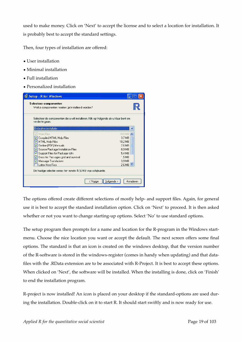
Then, four types of installation are offered:

• User installation

• Minimal installation

• Full installation

• Personalized installation

The options offered create different selections of mostly help- and support files. Again, for general

use it is best to accept the standard installation option. Click on ‘Next’ to proceed. It is then asked

whether or not you want to change starting-up options. Select ‘No’ to use standard options.

The setup program then prompts for a name and location for the R-program in the Windows start-

menu. Choose the nice location you want or accept the default. The next screen offers some final

options. The standard is that an icon is created on the windows desktop, that the version number

of the R-software is stored in the windows-register (comes in handy when updating) and that data-

files with the .RData extension are to be associated with R-Project. It is best to accept these options.

When clicked on ‘Next’, the software will be installed. When the installing is done, click on ‘Finish’

to end the installation program.

R-project is now installed! An icon is placed on your desktop if the standard-options are used dur-

ing the installation. Double-click on it to start R. It should start swiftly and is now ready for use.


Getting Packages

A freshly installed version of R-Project can do some pretty nice things already, but much more

functionality can be obtained by installing packages that contain new functions. These packages

are available by the internet and can be installed from within R-Project. Let’s say we want to use

the lme4-package, which can be used to estimate linear and generalized multilevel models. The

lme4-package does not come pre-installed with R-Project, so we have to download and install is

manually. The way this is done is shown based on an R-installation on windows XP.

Is the package installed?

Before we start to install a package, it is a good custom to check whether or not it is already in-

stalled. We start R-project and see the basic screen of the software. Choose ‘Packages’ from the

menu’s at the top of the screen. Six options are offered:


• Load Package: This is used to load packages that are already installed

• Set CRAN Mirror: Choose from which server the packages should be

downloaded

• Select repositories: Choose CRAN and CRAN (extras)

• Install package(s): Download and install new packages

• Update packages: Download new versions of already installed pack-

ages when available

• Install package(s) from local zip files: Used for computers not con-

nected to the internet

By selecting ‘Load Package’ we can check whether the ‘lme4′-package

we want is already installed. It appears not to. Click on ‘Cancel’ to return

to the main screen of P-Project. Note that some R-syntax is printed in red

in the R-Console window. This is the syntax that can be used to manu-

ally call for the window to selects packages to load.


Installing the package

Since the lme-package we want is not already installed, we are now going to do

this. Select ‘Packages’ from the menu at the top of the screen and then ‘Install

Package(s)…’. A window pops up asking us to choose a CRAN-mirror. This is

done only once during a session of R-Project. We have to choose where the pack-

age will be downloaded from and it is advisable to select one near the location

you’re at. I chose ‘Netherlands (Utrecht)’.

After a short while that is needed to download a list of the available packages

(internet connection is needed!), a new screen called ‘Packages’ pops forward and

allows the user to select a package to install. The length of the list gives an impres-

sion of the many packages available and the many ways R-Project can be extended

to fit your specific needs. I choose lme4 here and click on ‘OK’. The lme4-package

is downloaded and installed automatically and can be activated now. But first:

note that in some cases other packages are loaded as well. In this case the Matrix-

package is installed, because the requested lme4-package depends on it. This is

done to ensure a fully working version of R-Project at all times.

Loading the package

Now, the new package can be loaded and used. As described above, this can be

done by clicking on ‘Packages’ on the menu-bar at the top of the screen and then

on ‘Load Packages …’. It can be done manually as well using the following syntax:

library(lme4)

This loads the package and by default loads the packages it depends on as well if

these were not loaded already. In this case, the lattice-package (for trellis graphics)

and the Matrix-package are loaded automatically.

Getting Help

Concordant with the open source community, R-Project is accompanied by many

additional help functions. Most of them are freely available.

The help() - function

R-Project has a help function build in. This functionality is focused on informing

the user on the parameters function have. Almost for all functions some examples

are given as well.


A general help page is available, which contains several introductory documents as ‘An Introduction to R’,

‘Frequently Asked Questions’, and ‘The R Language Definition’. More advanced documents are made avail-

able as well, such as ‘Writing R Extensions’ and ‘R Internals’. This general help page is called for by entering:

help.start()

To obtain help on a specific function, you use help() with the name of the function between the brackets. For

instance, if you want help on the plot() function, use the following syntax:

help(plot)

This results in a page that gives a short definition of the function, shows the parameters of the function, links

to related functions, and finally gives some examples.

Freely available documents

More elaborate documents can be found on the website of R-Project (http://www.r-project.org) in the

documents section. This can be found by clicking on ‘manuals’ from the home-page, just below the ‘docu-

ments’ header. First, a couple of documents written by the core development team of R-Project are offered,

but don’t forget to click on the ‘Contributed Documentation’ link, which leads to many more documents,

often of a very high quality.

Books on R-Project

Many books have been written on R-Project, ranging from very basic-level introductions to the ones that ad-

dress the fundamental parts of the software. In this manual I review some of these books, which I can advise

to every starting or more advanced user of R-Project:

• Mixed-Effect Models in S and S-Plus, by José Pinheiro & Douglas Bates

• An R and S-PLUS Companion to Applied Regression, by John Fox

• Introductory Statistics with R, by Peter Dalgaard

• Data Analysis Using Regression and Multilevel / Hierarchical Models, by Andrew Gelman and Jennifer

Hill

R-help mailinglist

When all help fails, there is always the R-Help mailing-list. This is a service where all members receive the e-

mails that are send to a specific address. The quality and speed of the given answers and solutions is often

very high. Questions are asked and answered many times a day, so be prepared to receive a high volume of

e-mail when signing up for this service.

More information on the R-help mailing-list, as well as the ability to sign-up, can be found on:

https://stat.ethz.ch/mailman/listinfo/r-help


Conventions in this manual

The way this manual is manual is set up, is pretty straightforward. Often, a short introduction is

given on the subject at hand, after which one or more examples will follow. Since this manual

originated on the internet, where space is available unlimitedly, often many examples are given all

with slight variations. This is maintained in this version of the manual, for I believe that this makes

the makes clear the subtleties of the R language perfectly.

All the chapters can be read individually, for almost no prior knowledge is assumed at the start of

chapters. The only exception to this are some basics that are introduced in chapter 2 (Basics). Ex-

amples in paragraphs can build further on earlier examples from that paragraph, but will never

relate to examples of prior paragraphs. This again means, that the examples within a paragraph

can be read individually, without the need to refer backwards in the manual.

The examples in this manual are presented in R-syntax. This syntax is written inside light-grey boxes like this one. All the syntax can be copied directly into R and executed to see the results for yourself.

The results of the examples are given as well. This can be rec-ognized by these same font as is used for the syntax, but with-out the light-grey box around it. All the command from the syn-tax can be found in the output as well, preceded by the prompt ‘>’ that R uses to indicate that it is ready to accept new com-mands. The advantage of this is that it is easy to see what out-put is resulting from which command.


Chapter Two: Basics



Most Basic of All

In this section of my R manual, the most basic of the basics are introduced. Attention will be paid

to basic calculations, still the basis of every refined statistical analysis. Furthermore, storing data

and using stored data in functions is introduced.

Calculations in R

R can be used as a fully functional calculator. When R is started, some licensing information is

shown, as well as a prompt ( > ). When commands are typed and ENTER is pressed, R starts work-

ing and returns the outcome of the command. Probably the most basic command that can be en-

tered is a basic number. Since it is not stated what to do with this number, R simply returns it.

Some special numbers have names. When these names are called, the corresponding number is

returned. Finally, next to numbers, text can be handled by R as well.

33 * 23 ^ 2piapple“apple”

In the box above six commands were entered to the R prompt. These commands can be entered

one by one, or pasted to the R-console all at once. After these commands are entered one by one,

the screen looks like this:

> 3[1] 3> 3 * 2[1] 6> 3 ^ 2[1] 9> > pi[1] 3.141593> appleError: object “apple” not found> “apple”[1] “apple”

On the first row, we see after the prompt ( > ) our first ‘command’. The row below is used by R to

give us the result. The indication [1] means, that it is the first outcome that is first printed on that

row. This may seem quite obvious (which it is), but can become very useful when working with

larger sets of data.


The next few rows show the results of a few basic calculations. Nothing unexpected here. When PI

is called for, the expected number appears. This is because R has a set of these numbers available,

called constants. When an unknown name is called, an error message is given. R does not know a

number, or anything else for that matter, called apple. When the word apple is bracketed (” “), it is

seen as a character string and returned just like the numbers are.

Combining values

In statistics, we tend to use more than just single numbers. R is able to perform calculation on sets

of data in exactly the same way as is done with single numbers. This is shown below. Several

numbers can be combined into one ‘unit’ by using the c() command. C stands for concatenate. So,

as the two first commands below try to achieve, we can combine both numbers as well as character

strings. As said, we can use these ranges of data in our calculation. When we do so, shorter ranges

of data are iterated to match the length of the longer / longest range of data.

c(3,4,3,2)c(”apple”, “pear”, “banana”)

3 * c(3,4,3,2)c(1,2) * c(3,4,3,2)c(1,2,1,2) * c(3,4,3,2)

In the output below, we see that the first two commands lead to the return of the created units of

combined data. As above, we see the [1]-indicator, while four or three items are returned. This is

because R indicates the number / index of the first item on a row only. When we multiply the

range of four number by a single number (3), all the individual numbers are multiplied by that

number. In de final two command-lines, two numbers are multiplied by four number. This results

in a 2-fold iteration of the two numbers. So, the result of the two last commands are the same.

> c(3,4,3,2)[1] 3 4 3 2> c(”apple”, “pear”, “banana”)[1] “apple” “pear” “banana”> > 3 * c(3,4,3,2)[1] 9 12 9 6> c(1,2) * c(3,4,3,2)[1] 3 8 3 4> c(1,2,1,2) * c(3,4,3,2)[1] 3 8 3 4


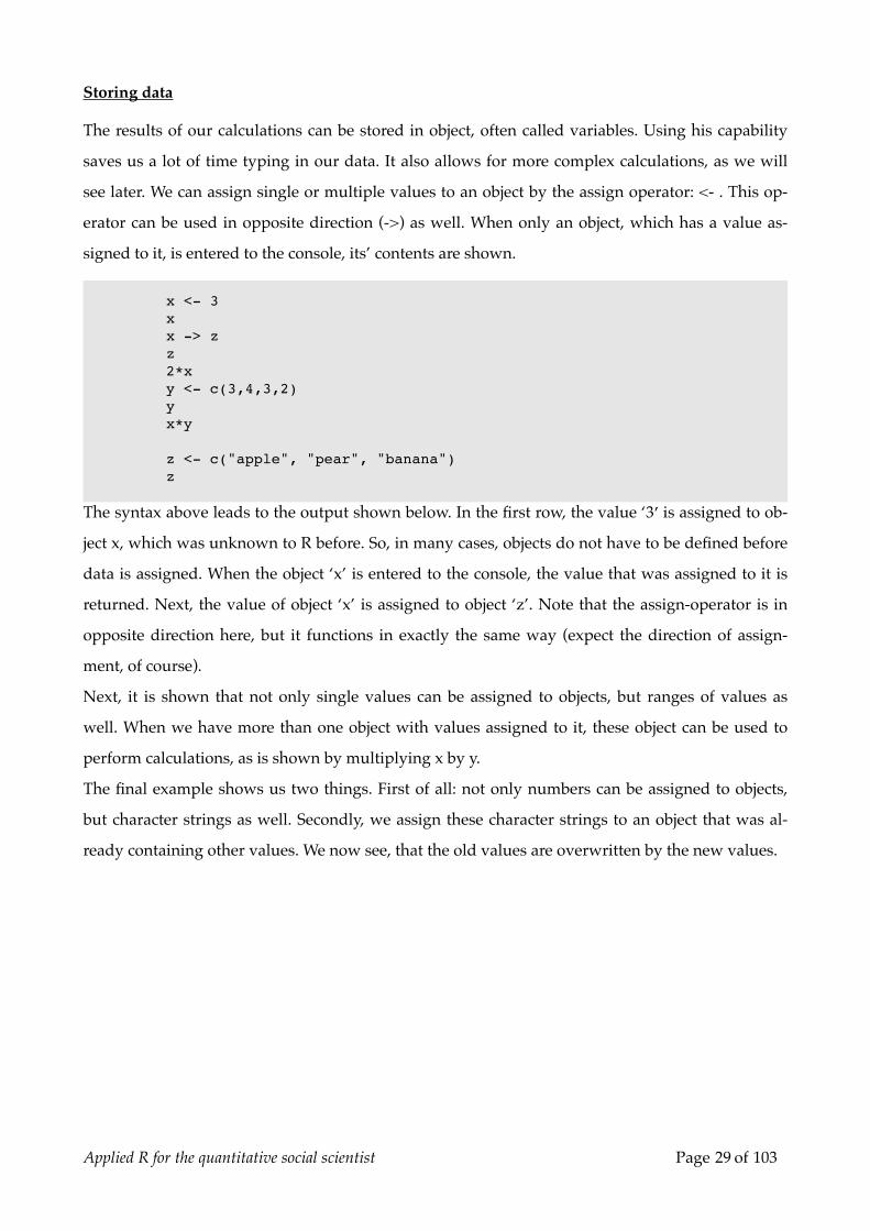
Storing data

The results of our calculations can be stored in object, often called variables. Using his capability

saves us a lot of time typing in our data. It also allows for more complex calculations, as we will

see later. We can assign single or multiple values to an object by the assign operator: <- . This op-

erator can be used in opposite direction (->) as well. When only an object, which has a value as-

signed to it, is entered to the console, its’ contents are shown.

x <- 3xx -> zz2*xy <- c(3,4,3,2)yx*y

z <- c("apple", "pear", "banana")z

The syntax above leads to the output shown below. In the first row, the value ‘3′ is assigned to ob-

ject x, which was unknown to R before. So, in many cases, objects do not have to be defined before

data is assigned. When the object ‘x’ is entered to the console, the value that was assigned to it is

returned. Next, the value of object ‘x’ is assigned to object ‘z’. Note that the assign-operator is in

opposite direction here, but it functions in exactly the same way (expect the direction of assign-

ment, of course).

Next, it is shown that not only single values can be assigned to objects, but ranges of values as

well. When we have more than one object with values assigned to it, these object can be used to

perform calculations, as is shown by multiplying x by y.

The final example shows us two things. First of all: not only numbers can be assigned to objects,

but character strings as well. Secondly, we assign these character strings to an object that was al-

ready containing other values. We now see, that the old values are overwritten by the new values.


> x <- 3 > x[1] 3> x -> z> z[1] 3> 2*x[1] 6> y <- c(3,4,3,2)> y[1] 3 4 3 2> x*y[1] 9 12 9 6> > z <- c("apple", "pear", "banana")> z[1] “apple” “pear” “banana”

Functions and stored data

Many of the object we create in R can be entered into the multitude of functions that are available.

A very straightforward function in mean(). As we can see in the syntax and the output below, this

function behaves exactly the same when a range of values or an object with that range of values is

entered. We also learn from these examples that the results of functions can be stored in objects as

well.

mean(c(3,4,3,2)) y <- c(3,4,3,2)mean(y)m <- mean(y)m

> mean(c(3,4,3,2))[1] 3> mean(y)[1] 3> m <- mean(y)> m[1] 3


Data Structure

The way R-Project handles data differs from some mainstream statistical programs, such as SPSS.

It can handle an unlimited number of data sets, as long as the memory of your computer can han-

dle it. Often, the results of statistical tests or estimation-procedures are stored inside ‘data-sets’ as

well. In order to be able to serve different needs, several different types of data-storage are avail-

able.

This paragraph will introduce some of the types of data-storage and shows how these objects are

managed by R-Project.

Single values and vectors

As was already shown in a previous paragraph, data can easily be stored inside objects. This goes

for single values and for ranges of values, called vectors. Below three variables values are created

(x, y, and z) where x will contain a single numerical value, y contains three numerical values and z

will contain two character values. This is done by using the c()-command that concatenates data.

Finally, in the syntax below, it is shown that it is not possible to concatenate different types of data

(i.e. numerical data and character data): when this is tried below, the numerical data are converted

into character-data.

x <- 3y <- c(4,5)z <- c("one", "two")xyz

c(x,y)c(x,y,z)

> x <- 3> y <- c(4,5)> z <- c("one", "two")> x[1] 3> y[1] 4 5> z[1] “one” “two”>> c(x,y)[1] 3 4 5> c(x,y,z)[1] “3″ “4″ “5″ “one” “two”


Matrix

Oftentimes, we want to store data in more than one dimension. This can be done with matrices,

that have two dimensions. As with vectors, all the data inside a matrix have to be of the same type.

a <- matrix(nrow=2, ncol=5)b <- matrix(data=1:10, nrow=2, ncol=5, byrow=FALSE)c <- matrix(data=1:10, nrow=2, ncol=5, byrow=TRUE)d <- matrix(data=c("one", "two", "three", "four", "five", "six"), nrow=3, ncol=2, byrow=TRUE)abcd

In the syntax above, four matrices are created and assigned to variables that were called ‘a’, ‘b’, ‘c’,

and ‘d’. The first matrix (’a') is created using the matrix() function. It is specified that this matrix

will have two rows (nrow=2) and five columns (ncol=5). In the output we see the resulting matrix:

all the data is missing, which is indicated by ‘NA’.

The following two matrices have data assigned to it by the ‘data=’ parameter. To both matrices the

values 1 to 10 are assigned, but in the first matrix ‘byrow=FALSE’ is specified and in the second

‘byrow=TRUE’. This results in a different way the data is entered into the matrix (row-wise or

column-wise), as can be seen below. The last matrix shows us, that character values can be stored

in matrices as well.

> a <- matrix(nrow=2, ncol=5)> b <- matrix(data=1:10, nrow=2, ncol=5, byrow=FALSE)> c <- matrix(data=1:10, nrow=2, ncol=5, byrow=TRUE)> d <- matrix(data=c("one", "two", "three", "four", "five", "six"), nrow=3, ncol=2, byrow=TRUE)> a [,1] [,2] [,3] [,4] [,5][1,] NA NA NA NA NA[2,] NA NA NA NA NA> b [,1] [,2] [,3] [,4] [,5][1,] 1 3 5 7 9[2,] 2 4 6 8 10> c [,1] [,2] [,3] [,4] [,5][1,] 1 2 3 4 5[2,] 6 7 8 9 10> d [,1] [,2][1,] “one” “two”[2,] “three” “four”[3,] “five” “six”


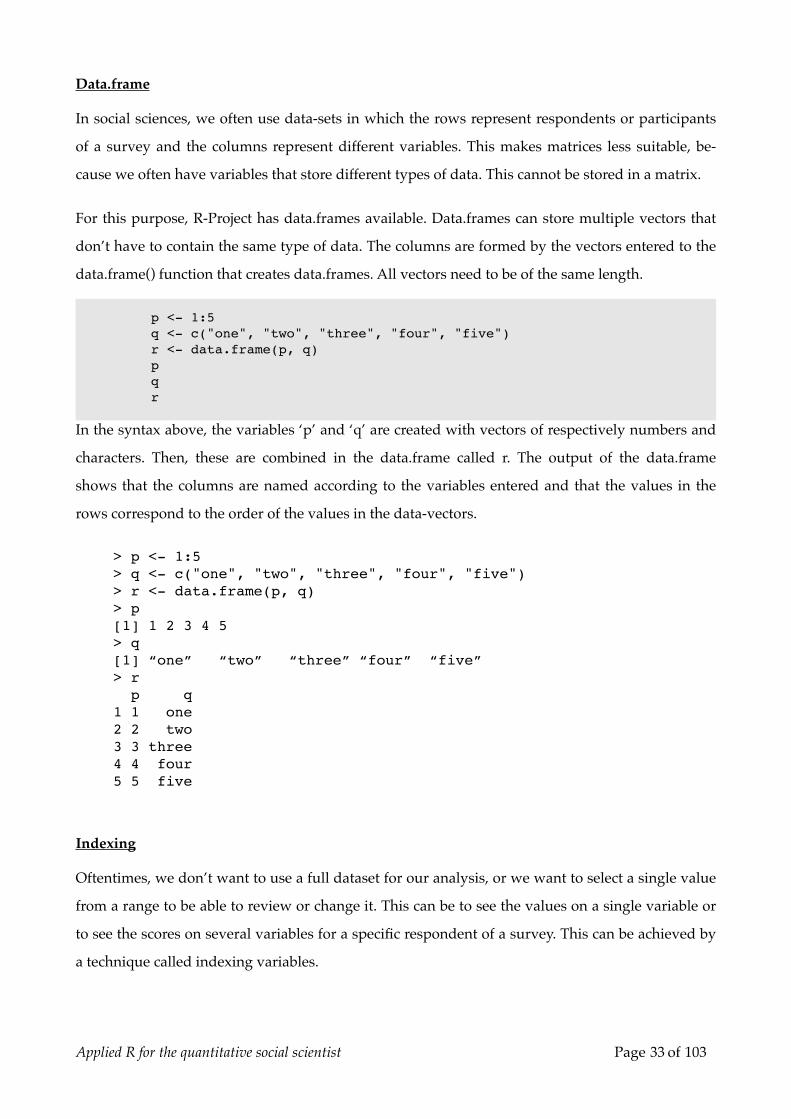
Data.frame

In social sciences, we often use data-sets in which the rows represent respondents or participants

of a survey and the columns represent different variables. This makes matrices less suitable, be-

cause we often have variables that store different types of data. This cannot be stored in a matrix.

For this purpose, R-Project has data.frames available. Data.frames can store multiple vectors that

don’t have to contain the same type of data. The columns are formed by the vectors entered to the

data.frame() function that creates data.frames. All vectors need to be of the same length.

p <- 1:5q <- c("one", "two", "three", "four", "five")r <- data.frame(p, q)pqr

In the syntax above, the variables ‘p’ and ‘q’ are created with vectors of respectively numbers and

characters. Then, these are combined in the data.frame called r. The output of the data.frame

shows that the columns are named according to the variables entered and that the values in the

rows correspond to the order of the values in the data-vectors.

> p <- 1:5> q <- c("one", "two", "three", "four", "five")> r <- data.frame(p, q)> p[1] 1 2 3 4 5> q[1] “one” “two” “three” “four” “five”> r p q1 1 one2 2 two3 3 three4 4 four5 5 five

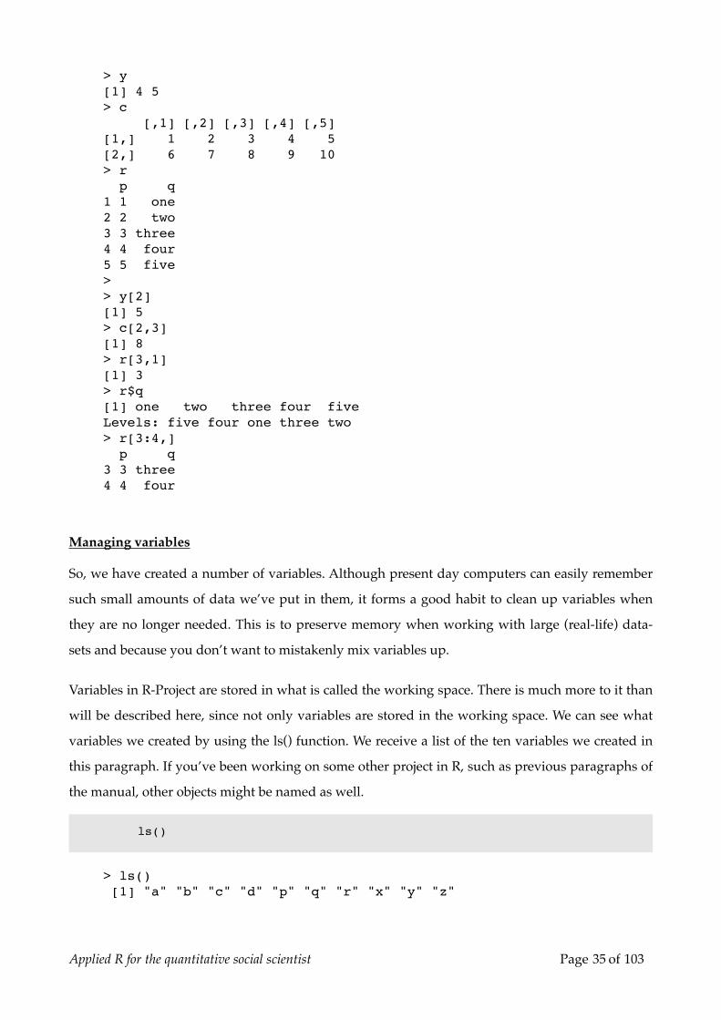
Indexing

Oftentimes, we don’t want to use a full dataset for our analysis, or we want to select a single value

from a range to be able to review or change it. This can be to see the values on a single variable or

to see the scores on several variables for a specific respondent of a survey. This can be achieved by

a technique called indexing variables.


Above, we’ve already created some variables of different types: a vector (’y'), a matrix (’c'), and a

data.frame (’r'). In the first rows of the syntax below these variables are called for, so we can see

what they look like.

ycr

y[2]c[2,3]r[3,1]r[3,]r$q

Then, they are indexed using straight brackets [ and ]. Since a vector has only one dimension, we

place the number or index of the value we want to see between the brackets that are placed behind

the name of the variable. In the syntax above, we want to see only the second value stored inside

vector ‘y’. In the output below we receive the value 5, which is correct.

A matrix has two dimensions and can be indexed using two values, instead of just one. For in-

stance, let’s sat we want to see the value on the second row on the third column stored in matrix

‘c’. We used the index [2,3] to achieve this (first the row number, then the column number). Below

we can see that this works out just fine.

Then the data.frame, which works almost the same as a matrix. First we want to see the value on

the third row of the first column and index the data.frame ‘r’ by using [3,1]. The result is as ex-

pected. When we want to see all the values on a specific variable, we can address this variable by

naming the data.frame in which it is stored, then a dollar-sign $ and finally the exact name of the

variable. This is done on the next row of the syntax, where we call for the variable ‘q’ inside

data.frame ‘r’.

The same can be achieved for a single row of the data.frame, giving the scores on all columns /

variables for one row / respondent. This is done by specifying the row we want, then a comma

and leaving the index for the row number open. We additionally show something else here: it is

not necessary to specify just a single value: a combination or range of values is fine as well. So:

here we want the values stored in all the columns of the data.frame for the third and fourth row.

We achieve this by indexing the data.frame ‘r’ using [3:4, ].


> y[1] 4 5> c [,1] [,2] [,3] [,4] [,5][1,] 1 2 3 4 5[2,] 6 7 8 9 10> r p q1 1 one2 2 two3 3 three4 4 four5 5 five>> y[2][1] 5> c[2,3][1] 8> r[3,1][1] 3> r$q[1] one two three four fiveLevels: five four one three two> r[3:4,] p q3 3 three4 4 four

Managing variables

So, we have created a number of variables. Although present day computers can easily remember

such small amounts of data we’ve put in them, it forms a good habit to clean up variables when

they are no longer needed. This is to preserve memory when working with large (real-life) data-

sets and because you don’t want to mistakenly mix variables up.

Variables in R-Project are stored in what is called the working space. There is much more to it than

will be described here, since not only variables are stored in the working space. We can see what

variables we created by using the ls() function. We receive a list of the ten variables we created in

this paragraph. If you’ve been working on some other project in R, such as previous paragraphs of

the manual, other objects might be named as well.

ls()

> ls() [1] "a" "b" "c" "d" "p" "q" "r" "x" "y" "z"


Now we want to clean up a bit. This can be done by using the rm() (rm = remove) function. Be-

tween the brackets the variables that need to be deleted are specified. We first delete all the vari-

ables, except the ones that were associated with creating the data.frame because we will need them

below. When a new ls() is called for, we see that the variables are gone.

rm(a,b,c,d,x,y,z)ls()rm(p,q)

> rm(a,b,c,d,x,y,z)> ls()[1] "p" "q" "r"> rm(p,q)

Remember that the variables ‘p’ and ‘q’ were stored inside the data.frame we called ‘r’. Therefor,

we don’t need them anymore. They are thus deleted as well.

Attaching data.frames

When working with survey data, as the quantitative sociologist often does, data.frames are often

the type of data-storage of choice. As we have already seen, variables stored in data.frame can be

addressed individually or group-wise. But in daily practice, this can become very tedious to be

typing all the indexes when working with specific (subsets of) variables. Fortunately it is possible

to bring the variables stored in a data.frame to the foreground by attaching them to the active

work-space.

ls()prattach(r)ls()prdetach(r)

In the syntax above, a list of the available data-objects is requested. We see in the output below that

only ‘r’ is available, which we remember to be a data.frame containing the variables ‘p’ and ‘q’.

When ‘p’ is called for directly, an error message is returned: object “p” is not to be found.

In such cases, we can tell R-Project where too look by indexing (as done above), or by attaching the

data.frame. This is done by the attach() function. When we request a list of available object again,


we still see only the data.frame ‘r’ coming up, but when object ‘p’ is requested, we now see it re-

turned. The data.frame can still be called for normally. Finally we can bring the data.frame back to

the ‘background’ by using the detach() function.

One word of notice: when working with an attached data.frame, it is very important to keep track

of changes made to the variables. The ‘p’-variable we could call for when the data.frame was at-

tached, is not the same as the ‘p’-variable stored inside the data.frame. So, changes made to the ‘p’-

variable when the data.frame is attached are lost when the data.frame is detached. This of course

does not hold when the changes are made directly to the variables inside the data.frame.

> ls()[1] "r"> pError: object "p" not found> r p q1 1 one2 2 two3 3 three4 4 four5 5 five> attach(r)> ls()[1] "r"> p[1] 1 2 3 4 5> r p q1 1 one2 2 two3 3 three4 4 four5 5 five> detach(r)


Getting Data into R

Various ways are provided to enter data into R. The most basic method is entering is manually, but

this tends to get very tedious. An often more useful way is using the read.table command. It has

some variants, as will be shown below. Another way of getting data into R is using the clipboard.

The back-draw thereof is the loss of some control over the process. Finally, it will be described how

data from SPSS can be read in directly.

Only basic ways of entering data into R are shown here. Much more is possible as other functions

offer almost unlimited control. Here the emphasis will be on day-to-day usage.

Reading data from a file

The most general of data-files are basically plain text-files that store the data. Rows generally rep-

resent the cases ( / respondents), although the top-row often will state the variable labels. The val-

ues these variables can take are written in columns, separated by some kind of indicator, often

spaces, commas or tabs. Another variant is that there is no separating character. In that case all

variables belonging to a single case are written in succession. Each variable then needs to have a

specific number of character places defined, to be able to distinguish between variables. Variable

labels are often left out on these type of files.

R is able to read all of the above-mentioned filetypes with the read.table() command, or its deriva-

tives read.csv() and read.delim(). The exception to this are fixed-width files. These are loaded using

the read.fwf() command, that uses different parameters. The derivatives of read.table() are basi-

cally the same command, but have different defaults. Because their use is so much convenience,

these will be used here.

Comma / Tab separated files

As said, the most generic way of reading data is the read.table() command. When given only the

filename as parameter, it treats a space as the separating character (so, beware on using spaces in

variable labels) and assumes that there are no variable names on the first row of the data. The

decimal sign is a “.”. This would lead to the first row of the syntax below, which assigns the con-

tents of a datafile “filename” to the object data, which becomes a data.frame.

The read.csv() and the read.delim() commands are basically the same, but they have a different set

of standard values to the parameters. Read.csv() is used for comma-separated files (such as, for

instance, Microsoft Excell can export to). The syntax for read.csv() is very simple, as shown below.


The read.table()-command can be used for the exact same purpose, by altering the parameters. The

header=TRUE - parameter means that the first row of the file is now regarded as containing the

variable names. The sep - parameter now indicates the comma “,” as the separating character.

fill=TRUE tells the function that if a row contains less columns than there are variables defined by

the header row, the missing variables are still assigned to the data frame that results from this func-

tion. Those variables for these cases will have the value ‘NA’ (missing). By dec=”.” the character

used for decimal points is set to a point (to not interfere with the separating comma). In contrast

with the read.table() function. the comment.char is disabled (set to nothing). Normally, if the

comment.char is found in the data, no more data is read from the row that is was found on (after

the sign, of course). In read.csv() this is disabled by default.

The last two rows of the syntax below shows the read.delim() command and the parameters

needed to create the same functionality from read.table. The read.delim() function is used to read

tab-delimited data. So, the sep-parameter is now set to “\t” by default. \t means tab. The other

parameters are identical to those that read.csv() defaults to.

data <- read.table("filename")

data <- read.csv("filename")data <- read.table("filename", header = TRUE, sep = ",", dec=".", fill = TRUE, comment.char="")

data <- read.delim("filename")data <- read.table("filename", header = TRUE, sep = "\t", dec=".", fill = TRUE, comment.char="")

Variable labels

Data that is read into a data.frame can be given variable names. For instance, if the above com-

mands were used to read a data-file containing three variables, variable names can be assigned in

several ways. Two ways will be described here: assigning them after the data is read or assigning

them using the read.table() command.

names(data) <- c("Age","Income","Gender") data <- read.table("filename", colnames=c("Age","Income","Gender"))

In the syntax above, the names() command is used to assign names to the columns of the

data.frame (representing the variables). The names are given as strings (hence the apostrophes)

and gathered using the c() command.


Fixed width files

When reading files in the ‘fixed width’ format, we cannot rely on a single character that indicates

the separations between variables. Instead, the read.fwf() function has a parameter by which we

tell the function where to end a variable and start the next one. Just as with read.table(), a

data.frame is returned. Variable labels are treated the same way as the previous mentioned

data <- read.fwf("filename", widths = c(2,5,1), colnames=c("Age", "Income", "Gender"))data <- read.fwf("filename", widths = c(-5,2,5,-2, 1), colnames=c("Age", "Income", "Gender"))

Reading data from the clipboard

data <- read.table(pipe("pbpaste"))data <- read.table("clipboard")

Read.table is used for read comma seperated files. read.delim is used for reading tab delimited

files. read.table(pipe(”pbpaste”)) is used for reading data from the clipboard on mac. read.table

(”clipboard”) is used for reading data from the clipboard on Windows. Instead of read.table(pipe

(”pbpaste”)) you can use read.delim(pipe(”pbpaste”)) as well.

Reading data from other statistical packages {foreign}

library(foreign)data <-read.spss("filename")

library(foreign) loads the foreign package, which contains the read.spss() function, which can read

data as written by the SPSS software.


Data Manipulation

Recoding

The most direct way to recode data in R-Project is using a combination of both indexing and condi-

tionals as described elsewhere. To exemplify this, a simply data.frame will be created below, con-

taining variables indicating gender and monthly income in thousands of euros.

gender <- c("male", "female", "female", "male", "male", "male", "female")income <- c(54, 34, 556, 57, 88, 856, 23)data <- data.frame(gender, income)data

> gender <- c("male", "female", "female", "male", "male", "male", "female")> income <- c(54, 34, 556, 57, 88, 856, 23)> data <- data.frame(gender, income)> data gender income1 male 542 female 343 female 5564 male 575 male 886 male 8567 female 23

Some of the values on the income variable seem exceptionally high. Let’s say we want to remove

the two values on income higher than 500. In order to do so, we use the which() command, that

reveals which of the values is greater than 500. Next, the result of this is used for indexing the da-

ta$income variable. Finally, the indicator for missing values, ‘NA’ is assigned to the that selected

values of the ‘income’ variables. Obviously, we would normally only use the third line. The first

two are shown here, to make clear exactly what is happening.

which(data$income > 500)data$income[data$income > 500]data$income[data$income > 500] <- NAdata


> which(data$income > 500)[1] 3 6> data$income[data$income > 500][1] 556 856> data$income[data$income > 500] <- NA> data gender income1 male 542 female 343 female NA4 male 575 male 886 male NA7 female 23

Sometimes, it is desirable to replace missing values by the mean on the respective variables. That is

what we are going to do here. Note, that in general practice it is not very sensible to impute two

missing values using only five valid values. Nevertheless, we will proceed here.

The first row of the example below shows that it is not automatically possible to calculate the mean

of a variable that contains missing values. Since R-Project cannot compute a valid value, NA is re-

turned. This is not what we want. Therefore, we instruct R-Project to remove missing values by

adding na.rm=TRUE to the mean() command. Now, the right value is returned. When the same

selection-techniques as above are used, an error will occur. Therefore, we need the is.na() com-

mand, that returns a vector of logicals (’TRUE’ and ‘FALSE’ ). Using is.na(), we can use the which()

command to select the desired values on the income variable. To these, the calculated mean is as-

signed.

mean(data$income)mean(data$income, na.rm=TRUE)data$income[which(is.na(data$income))] <- mean(data$income, na.rm=TRUE)data

> mean(data$income)[1] NA> mean(data$income, na.rm=TRUE)[1] 51.2> data$income[which(is.na(data$income))] <- mean(data$income, na.rm=TRUE)> data gender income1 male 54.02 female 34.03 female 51.24 male 57.05 male 88.06 male 51.27 female 23.0


Order

It is easy to sort a data-frame using the command order. Combined with indexing functions, it

works as follows:

x <- c(1,3,5,4,2)y <- c('a','b','c','d','e')df <- data.frame(x,y)df

x y1 1 a2 3 b3 5 c4 4 d5 2 e

df[order(df$x),] x y1 1 a5 2 e2 3 b4 4 d3 5 c

Merge

Merge puts multiple data.frames together, based on an identifier-variable which is unique or a

combination of variables.

x <- c(1,2,5,4,3)y <- c(1,2,3,4,5)z <- c('a','b','c','d','e')df1 <- data.frame(x,y)df2 <- data.frame(x,z)df3 <- merge(df1,df2,by=c("x"))df3

df3 x y z1 1 1 a2 2 2 b3 3 5 e4 4 4 d5 5 3 c


Tables

Most basic functions used are probably those of creating tables. These can be created in multiple

ways.

Tapply

The function TAPPLY can be used to perform calculations on table-marginals. Different functions

can be used, such as MEAN, SUM, VAR, SD, LENGTH (for frequency-tables). For example:

x <- c(0,1,2,3,4,5,6,7,8,9)y <- c(1,1,1,1,1,1,2,2,2,2)tapply(x,y,mean)tapply(x,y,sum)tapply(x,y,var)tapply(x,y,length)

> x <- c(0,1,2,3,4,5,6,7,8,9)> y <- c(1,1,1,1,1,1,2,2,2,2)> tapply(x,y,mean) 1 22.5 7.5> tapply(x,y,sum) 1 215 30> tapply(x,y,var) 1 23.500000 1.666667> tapply(x,y,length)1 26 4>

Ftable

More elaborate frequency tables can be created with the FTABLE-function. For example:

x <- c(0,1,2,3,4,5,6,7,8,9)y <- c(1,1,1,1,1,1,2,2,2,2)z <- c(1,1,1,2,2,2,2,2,1,1)ftable(x,y,z)


> x <- c(0,1,2,3,4,5,6,7,8,9)> y <- c(1,1,1,1,1,1,2,2,2,2)> z <- c(1,1,1,2,2,2,2,2,1,1)> ftable(x,y,z) z 1 2x y0 1 1 0 2 0 01 1 1 0 2 0 02 1 1 0 2 0 03 1 0 1 2 0 04 1 0 1 2 0 05 1 0 1 2 0 06 1 0 0 2 0 17 1 0 0 2 0 18 1 0 0 2 1 09 1 0 0 2 1 0

Conditionals

Conditionals, or logicals, are used to check vectors of data against conditions. In practice, this is

used to select subsets of data or to recode values. Here, only some of the fundamentals of condi-

tionals are described.

Basics

The general form of conditionals are two values, or two sets of values, and the condition to test

against. Examples of such tests are ‘is larger than’, ‘equals’, and ‘is larger than’. In the example be-

low the values ‘3′ and ‘4′ are tested using these three tests.

3 > 43 == 43 < 4


> 3 > 4[1] FALSE> 3 == 4[1] FALSE> 3 < 4[1] TRUE

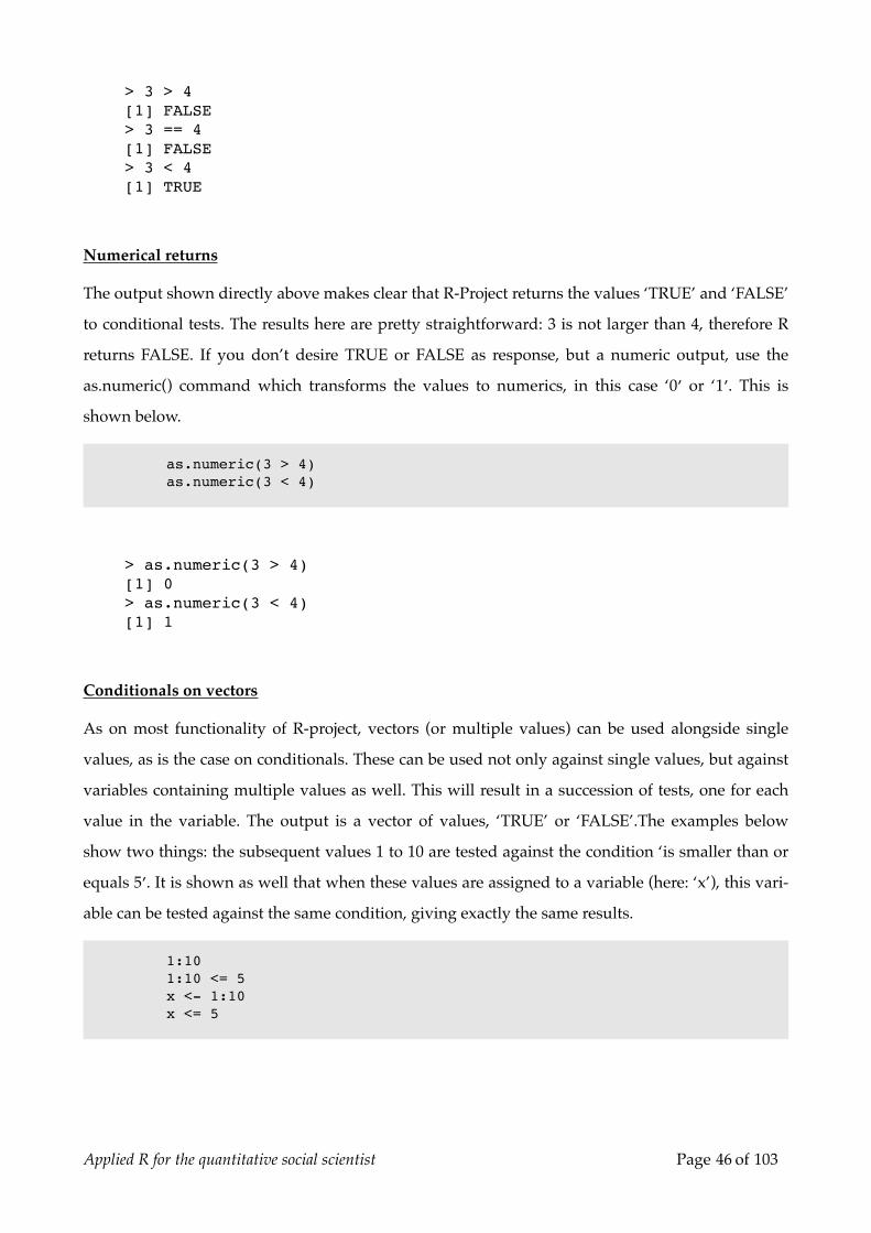
Numerical returns

The output shown directly above makes clear that R-Project returns the values ‘TRUE’ and ‘FALSE’

to conditional tests. The results here are pretty straightforward: 3 is not larger than 4, therefore R

returns FALSE. If you don’t desire TRUE or FALSE as response, but a numeric output, use the

as.numeric() command which transforms the values to numerics, in this case ‘0′ or ‘1′. This is

shown below.

as.numeric(3 > 4)as.numeric(3 < 4)

> as.numeric(3 > 4)[1] 0> as.numeric(3 < 4)[1] 1

Conditionals on vectors

As on most functionality of R-project, vectors (or multiple values) can be used alongside single

values, as is the case on conditionals. These can be used not only against single values, but against

variables containing multiple values as well. This will result in a succession of tests, one for each

value in the variable. The output is a vector of values, ‘TRUE’ or ‘FALSE’.The examples below

show two things: the subsequent values 1 to 10 are tested against the condition ‘is smaller than or

equals 5′. It is shown as well that when these values are assigned to a variable (here: ‘x’), this vari-

able can be tested against the same condition, giving exactly the same results.

1:101:10 <= 5x <- 1:10x <= 5


> 1:10 [1] 1 2 3 4 5 6 7 8 9 10> 1:10 <= 5 [1] TRUE TRUE TRUE TRUE TRUE FALSE FALSE FALSE FALSE FALSE> x <- 1:10> x == 5 [1] TRUE TRUE TRUE TRUE TRUE FALSE FALSE FALSE FALSE FALSE

Conditionals and multiple tests

More tests can be gathered into one conditional expression. For instance, building on the example

above, the first row of the next example tests the values of variable ‘x’ against being smaller than

or equal to 4, or being larger than or equal to ‘6′. This results in ‘TRUE’ for all the values, except for

5. Since the ‘|’-operator is used, only one of the set conditions need to be true.

The second row of this example below tests the same values against two conditions as well,

namely ‘equal to or larger than 4′ and ‘equal to or smaller than 6′. since this time the ‘&’-operator

is used, both conditionals need to be true.

x <= 4 | x >= 6x >= 4 & x <= 6

> x <= 4 | x >= 6 [1] TRUE TRUE TRUE TRUE FALSE TRUE TRUE TRUE TRUE TRUE> x >= 4 & x <= 6 [1] FALSE FALSE FALSE TRUE TRUE TRUE FALSE FALSE FALSE FALSE

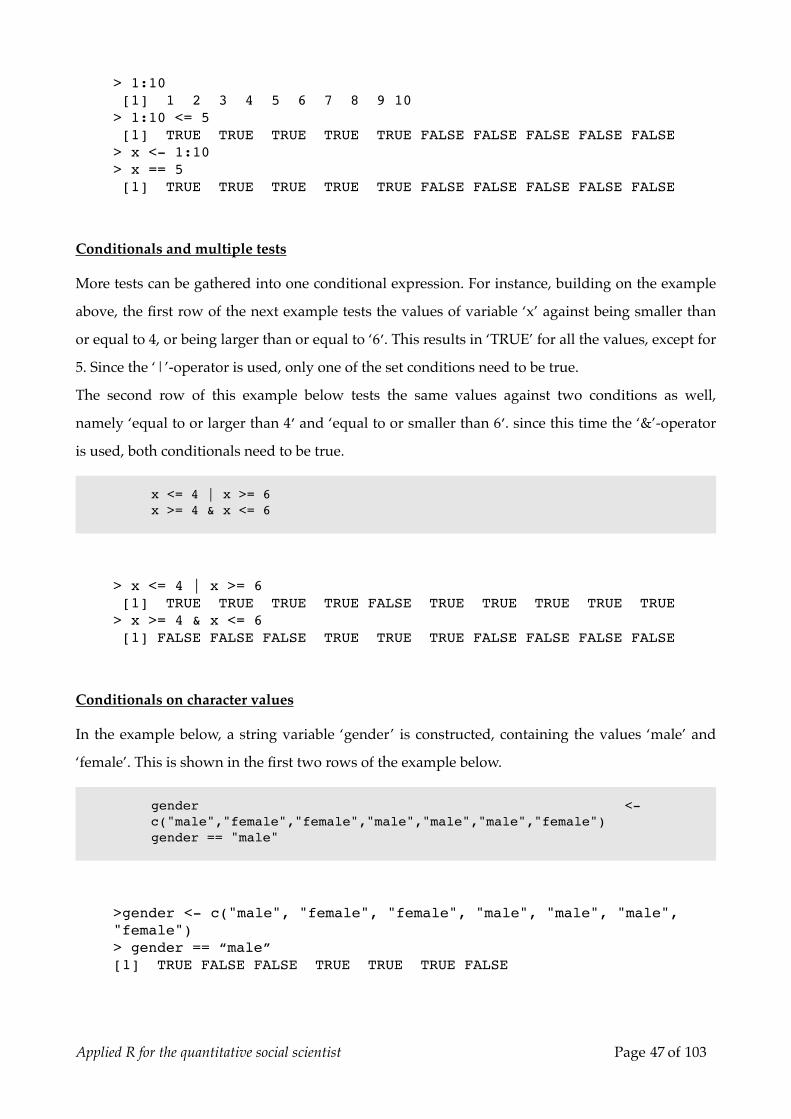
Conditionals on character values

In the example below, a string variable ‘gender’ is constructed, containing the values ‘male’ and

‘female’. This is shown in the first two rows of the example below.

gender <- c("male","female","female","male","male","male","female")gender == "male"

>gender <- c("male", "female", "female", "male", "male", "male", "female")> gender == “male”[1] TRUE FALSE FALSE TRUE TRUE TRUE FALSE


Additional functions

The last examples demonstrate two other functions using conditionals, using the same ‘gender’

variable as above.

The first is an additional way to get a numerical output of the same test as in the row above. The

iselse() command has three arguments: the first is a conditional, the second is the desired output if

the conditional is TRUE, the third is the output in case the result of the test is ‘FALSE’.

The second example shows a way to obtain a list of which values match the condition tested

against. In the output above, the second, third and last values are ‘female’. Using which() and the

condition “== ‘male’ ” (equals ‘male’) returns the indices of the values in variable ‘gender’ that

equal ‘male’.

ifelse(gender==”male”,0,1)which(gender==”male”)

> ifelse(gender=="male",0,1)[1] 0 1 1 0 0 0 1> which(gender=="male")[1] 1 4 5 6

Conditionals on missing values

Missings values (’NA’) form a special case in many ways, such as when using conditionals. Nor-

mal conditionals cannot be used to find the missing values in a range of values, as is shown below.

x <- c(4,3,6,NA,4,3,NA)x == NAwhich(x == NA)

is.na(x)which(is.na(x))

The last two rows of the syntax above show what can be done. The is.na() command tests whether

a value or a vector of values is missing. It returns a vector of logicals (’TRUE’ or ‘FALSE’), that in-

dicates missing values with a ‘TRUE’. Nesting this command in the which() command described

earlier enables us to find which of the values are missing. In this case, the fourth and the seventh

values are missing.


> x <- c(4,3,6,NA,4,3,NA)> x == NA[1] NA NA NA NA NA NA NA> which(x == NA)integer(0)> is.na(x)[1] FALSE FALSE FALSE TRUE FALSE FALSE TRUE> which(is.na(x))[1] 4 7



Chapter Three: Graphics



Basic Graphics

Producing graphics can be a way to get familiar with your data or to strongly present your results.

Fortunately, this can be done both easy as well as in a very powerful way in R-Project. R-Project

comes with some standard graphical functions and a package for Trellis-graphics. Here, we will

see some of the basics of the standard graphics functionality of R-Project.

R-Project creates graphics and presents them in a ‘graphics device’. This can be a window on the

screen, but just as easily a file in a specified format (such as .bmp or .pdf). There are two types of

functions that create graphics in R-Project. One of those sets up such a graphics device by calculat-

ing and drawing the axes, plot title, margins and so on. Then the data is plotted into the device.

The other type of graphics function cannot create a graphics device and only adds data to a plot.

This paragraph shows only the first type of plotting-functions.

Basic Plotting

The most basic plot-function in R-Project is called ‘plot()’. It is a function that sets up the graphics-

device and is able to create some different types of graphic representations of your data.

For instance, let’s say we want to visualize a set of five values: 3,4,5,6 and 5. In the syntax below,

these values are first assigned to the variable ‘y’. Then, we call the plot()-function and tell it to plot

the data assigned to y.

y <- c(3,4,5,6,5)plot (y)plot (y, type=”l”, main=”Example line-plot”, xlab=”Predictor Value”, ylab=”Outcome Value”)

Although the syntax of the first plot-command is very sim-

ple, R-Project actually performs quite a bit of work for us. For

example: a new window opens, the plotting area is set along-

side margins, minimal and maximum values for the axes are

calculated based on the data and drawn succeedingly, basic

labels are added to the aces and finally: the data is repre-

sented. Obviously this plot is not ready for publication, but

fortunately all the ‘choices’ R-Project made for us are only the

defaults, so we can easily specify exactly what we want.


The next plot already looks a bit better. This is because some

extra specifications are added to the second plot-command in

the syntax above. By specifying “type=”l” we tell the plot-

function that we want the data-points to be connected using

a line. The main=” ” specification creates a header for the

plot, while the xlab=” ” and ylab=” ” specify the labels for

the x-axis and y-axis respectively.

x <- c(1,3,4,7,9)plot (x,y, type=”b”, main=”Example plot”, xlab=”Predictor Value”, ylab=”Outcome Value”)

What if the values that we want to represent are related to

predictor values (values on the x-axis) that are not evenly

spread, such as in the graphics above? In that case, we have

to specify the values on the x-axis to the plot()-function. The

syntax above shows how this is done. First, we assign some

values to the variable we call x. Then, we replicate the plot()-

syntax from above and add the x-variable to it, before the y-

variable. Additionally the type=”l” from above is changed

into type=”b” (b stands for both), which results in plotting

both a line as well as points. The plot this results in, is shown

to the right.

Other types of plots

Statistics does not exist solely out of line- and points-graphics. The syntax below shows how the

represent the data stored in the y-variable can be represented using a barplot, pie-chart, histogram

and a boxplot. These types of graphics are only shown, not described exhaustingly. All of these

functions have many parameters that can be used to create exactly what you want.

barplot(y, main=”Barplot”, names.arg=c(”a”,”b”,”c”,”d”,”e”))pie(y, main=”Pie-chart”, labels=c(”a”,”b”,”c”,”d”,”e”))hist(y, main=”Histogram”)boxplot(y, main=”Boxplot”)


The syntax above results almost exactly in the graph shown

to the right. The only difference is, that normally R-Project

would create four separate graphs when the syntax above is

provided. For an explanation of how to place more graphs on

one graphics device, see elsewhere in this manual.

All the graphics functions shown here have the main=” ” ar-

gument specified. The barplot() function has the additional

names.arg - argument specified, which here provides five let-

ters (”a” to “e”) as labels for the bars. On the pie-chart this is

done as well, but with the label-argument.

Intermediate Graphics

Based on the basic graphics that were created in the previous paragraph of this manual, we will

elaborate some to create more advanced graphics. What we are going to do is to add two other sets

of data, one represented by an additional line, one as four large green varying symbols. Then, in

order to keep oversight over the graph, a basic legend is added to the plot. Finally, we let R draw a

curved line based on a quadratic function.

Adding elements to plots

Just as in the previous paragraph, first some data will be created. The x and y variables are copied

from the previous paragraph, so we will be able to recreate the graph we saw there. Then, an addi-

tional set of values is created and assigned to the variable z. This is done in the first three rows of

the syntax below.

x <- c(1, 3, 4, 7, 9)y <- c(3, 4, 5, 6, 5)z <- c(5, 6, 4.5, 5.5, 5)

plot (x,y, type=”b”, main=”Example plot”, xlab=”Predictor Value”,ylab=”Outcome Value”, col=”blue”, lty=2)

lines(x, z, type=”b”, col=”red”)

points(x=c(2,4,6,8), y=c(5.5, 5.5, 5.5, 5.5), col=”darkgreen”, pch=1:4, cex=2)


Then, using the plot() function, a plot is created for the

first line we want, closely representing the figure from the

previous paragraph. Two things are different now: first of

all, we ask for a blue line, by specifying col=”blue”.

Secondly a dotted line is created because the line-type is

set to ‘2′ (lty=2).

Now we want to add an additional line. As you might

have noticed by now, the plot() function generally clears

the graphics-device and creates a new graphic from

scratch2. Remember that there are two types of plotting

functions: those that create a full plot (including the

preparation of the graphics device), and those that only

add elements to an already prepared graphics device. We

will use two functions of that second type to add elements

to our existing plot.

First, we want another line-graph, representing the rela-

tionship between the x and the z variables. For this, we

use the lines() function. By specifying col=”red” we get a

red line, added to our existing graph. It is possible to set

the line-type (which we didn’t here), but you can’t set

elements as labels for the axes or the main graph-title. This

can only be done by functions that setup the graphics de-

vice as well, such as plot().

Next, using points(), we add four green points to our al-

ready existing graphic. Instead of storing the four coordi-

nates of these points in variables and specifying these

variables in a plot-function, we describe the coordinates

inside the points() function. This can be done with all

(plotting) functions in are that require data, just as all these

functions can have data specified by using variables in


2 This is not always the case, though. You can have the plot() function add elements to existing graphs by specifying ‘add=TRUE’, which results in similar functionality as the lines() and points() functions shown here

which the data is stored. By specifying four different values for the ‘pch’-parameter, four different

symbols are used to indicate the data-points. The ‘cex=2′ parameter tells R to expand the standard

character in size by a factor 2 (cex stands for Character Expansionfactor).

Legend

legend(x=7.5, y=3.55, legend=c(”Line 1″, “Line 2″, “Dots”), col=c(”blue”,”red”, “darkgreen”), lty=c(2,1,0), pch=c(1,1,19))

A legend is not automatically added to graphics made by R-

Project. Fortunately, we can add these manually, by using the

legend() function. The syntax above is used to create the leg-

end as shown below.

Several parameters are needed to have the right legend

added to your graph. In the order as specified above these

are:

• x=7.5, y=3.55: These parameters specify the coordinates of

the legend. Normally, these coordinates refer to the upper-

left corner of the legend, but this can be specified differently.

• legend=c(”Line 1″, “Line 2″, “Dots”): the ‘legend=’ parameter needs to receive values that will

be used as labels in the legend. Here, I chose to use the character strings ‘Line 1′, ‘Line 2′, and

‘Dots’ and concatenated them using c(). It is important to note that the order these labels will ap-

pear on the legend is determined by the order that they are specified to the legend-parameter,

not by the order in which they are added to the plot.

• col=c(”blue”,”red”, “darkgreen”), lty=c(2,1,0), pch=c(1,1,19): The last three parameters, col, lty,

and pch, are treated the same way as in other graphical function, as described above. The differ-

ence is that not one value is given, but three.


Plotting the curve of a formula

Sometimes you don’t want to graphically represent data, but

the model that is based on it. Or, more generally, you want to

graphically represent a formula. When the relationship is bi-

variate, this can easily be done with the curve()-function. For

instance, let’s say we want to add the formula “y = 2 + x ^ 5″

(the result is 2 plus the square root of the value of x). Using

the syntax below, this formula is graphically represented and

added to the existing graphic. It is drawn for the values on

the x-axis from 1 to 7. Here it can be seen, that it is not neces-

sary to draw the function over the full scale of the x-scale. By

specifying lwd=2 (lwd= Line Width) a thick line is drawn.

curve(1 + x ^.5, from=1, to=7, add=TRUE, lwd=2)

Overlapping data points

In many cases, multiple points on a scatterplot have exactly the same coordinates. When these are

simply plotted, the visual representation of the data may be unsatisfactory. For instance, regard the

following data and plot:

x <- c(1, 1, 1, 2, 2, 2, 2, 2, 3, 4, 5, 3, 4)y <- c(5, 5, 5, 4, 4, 4, 4, 4, 3, 4, 2, 2, 2)

data.frame (x, y)

> data.frame(x,y) x y1 1 52 1 53 2 44 2 45 2 46 2 47 2 48 3 39 4 410 5 211 1 512 3 213 4 2


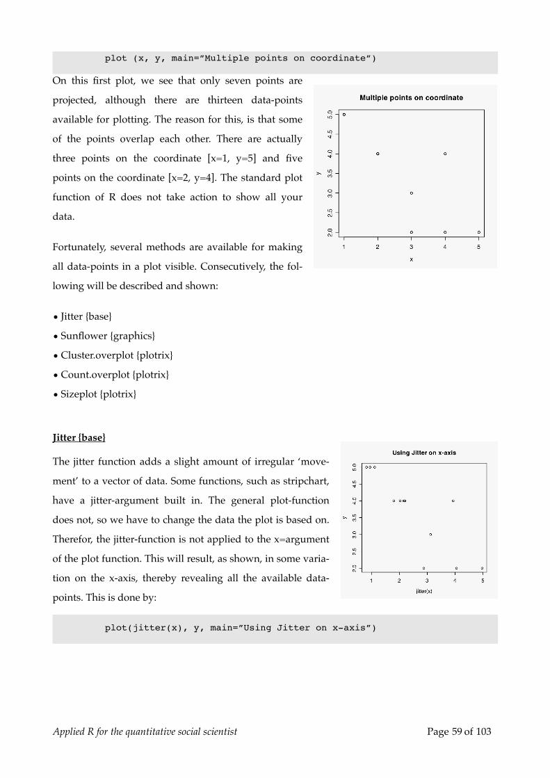
plot (x, y, main=”Multiple points on coordinate”)

On this first plot, we see that only seven points are

projected, although there are thirteen data-points

available for plotting. The reason for this, is that some

of the points overlap each other. There are actually

three points on the coordinate [x=1, y=5] and five

points on the coordinate [x=2, y=4]. The standard plot

function of R does not take action to show all your

data.

Fortunately, several methods are available for making

all data-points in a plot visible. Consecutively, the fol-

lowing will be described and shown:

• Jitter {base}

• Sunflower {graphics}

• Cluster.overplot {plotrix}

• Count.overplot {plotrix}

• Sizeplot {plotrix}

Jitter {base}

The jitter function adds a slight amount of irregular ‘move-

ment’ to a vector of data. Some functions, such as stripchart,

have a jitter-argument built in. The general plot-function

does not, so we have to change the data the plot is based on.

Therefor, the jitter-function is not applied to the x=argument

of the plot function. This will result, as shown, in some varia-

tion on the x-axis, thereby revealing all the available data-

points. This is done by:

plot(jitter(x), y, main=”Using Jitter on x-axis”)


As we can see, all three data-points on x=1 are clearly visible. But, the points on x=2 still clutter

together. So, when to many points overlap each other, jittering on just one axis might be not

enough. Fortunately, we can jitter more than just one axis:

plot(jitter(x), jitter(y), main=”Using Jitter on x- and y-axis”)

Now, we see the overlapping points varying slightly over

both the x-axis and the y-axis. All of the points are now

clearly visible. Nevertheless, if many more data-points were

plotted, again cluttering would occur. But, although not all

individual points will then be shown, using jitter still allows

for a better impression of the density of points in a region.

Sunflower {graphics}

sunflowerplot(x, y, main=”Using Sunflowers”)

Sunflower are often seen in the graphics produced by statisti-

cal packages. When more than a one point is to be drawn on

a single coordinate, a number of ‘leafs’ of the sunflower are

drawn, instead of the points that is to be expected. The ad-

vantage of this is the increased accuracy, but the back-draw is

that is works only when relatively few points need to be

drawn on one coordinate. Another back-draw of the method

is that the sunflowers take quite a lot of place, so overlapping

might occur if several points are to be plotted very close to each other.


Cluster.overplot {plotrix}

The next three examples are coming from functions inside

the plotrix package. The first of these functions is

cluster.overplot(). This function clusters up to nine overlap-

ping points of data. Therefor, this function is ideal for rela-

tively small data-sets. Due to the tight clustering, the plot is

not easily mistaken for showing randomness that is ‘real’ in

the data.

The functions itself does not plot data, but will return a list

with ‘new’ coordinates which can be plotted succeedingly. In the code below, first the plotrix pack-

age is loaded. Next, the list with new coordinates will be shown. Finally, cluster.overplot() function

is nested in the plot()-function, which leeds to the following plot:

require(plotrix)cluster.overplot(x,y)plot(cluster.overplot(x, y ), main=”Using cluster.overplot”)

Count.overplot {plotrix}

We have seen, that all of the methods that were described

above still rely on a visual representation of each overlapping

point of data. This still can result in very dense plots that are

hard to interpret. The next few methods try to solve this

problem.

The function count.overplot tries to give a more accurate rep-

resentation of overlapping data by not plotting every point

on slightly altered coordinates, but by placing a numerical

count of the overlapping data-points on the right coordinate. This results in a very accurate plot,

which still may be difficult to interpret, though. Using this method will result in a plot that does

not give us a feel of the localized density of the data and thereby may be misrepresenting the data.

It should only be used when described extensively.

count.overplot(x, y, main=”Using count.overplot”, xlab=”X-Axis”, ylab=”Y-Axis”)


Sizeplot {plotrix}

The next method adjusts the size of the plotted points. Since

the relation between number of overlapping points and the

increase in size can be adjusted, this method is suitable for

large sets of data.

sizeplot(x, y, main=”Using sizeplot”, xlab=”X-Axis”, ylab=”Y-Axis”)

Multiple Graphs

Sometimes it takes more than just one graph to illustrate your arguments. In those cases, you’ll of-

ten want these graphs to be held closely together in the output. R has several ways of doing so. In

the results that can be achieved with them, they differ a great deal, but their syntax differs only

slightly. These different functions cannot be used together on the same graph-window though.

As is traditional on this website, all the examples used will be fully self-contained. So, first some

data is assigned to objects. Then, a hypothetical case will be used of a ‘project’ to compare several

methods of graphing the same data. Let’s say that we want to make a plot, containing four types of

graphs next to each other: a scatterplot, a barchart, a pie-chart and a boxplot.

x1 <- c(4, 3, 4, 3, 4, 5, 4, 5, 6, 5, 5, 6, 7, 6, 7, 8 )x2 <- c(8, 7, 8, 7, 8, 7, 6, 5, 5, 6, 5, 4, 4, 5, 4, 3 )x3 <- c(1, 2, 1, 2, 1, 2, 3, 3, 3, 3, 3, 4, 4, 4, 4, 4 )x4 <- c(1, 2, 3, 4, 8, 7, 8, 9, 7, 6, 5, 4, 3, 3, 2, 1 )df <- data.frame(x1, x2, x3, x4)


Par(mfrow) {graphics}

The par (parameter) command from the graphics package

lets you set (or read) graphical parameters. It’s mfrow sub-

command sets the number of rows and columns the plotting

device will be divided in. In the example below, a vector of

c(2,2) is entered to the mfrow subcommand. Subsequently,

four plots are made as usual. Finally, the graphical parameter

is set to normal again by entering the vector c(1,1) to the

mfrow subcommand.

par(mfrow=c(2, 2))pie(mean(df),main=”Pie-chart”)barplot(mean(df), main=”Barplot”)boxplot(df, main=”Boxplots”)matplot(df,type=”l”, main=”Line diagram”)par(mfrow=c(1, 1))

Layout {Graphics}

The mfrow-parameter that was described above has the

drawback that all plots need to have identical dimensions,

while we might want, for instance, the line diagram to take

more place. In order to be able to do that, we must use the

layout() function, that divides a graphical device in separate

parts that can be plotted on succeedingly. The layout() func-

tion takes a matrix as an argument. This matrix contains

number that correspond to the numbered screens the graph-

ics device will be divided in. Parts with the same number

will be regarded as belonging together.

To create the example shown to the right, we will need four screens. We chose to make one screen

on the bottom quite large, the other three screens will be smaller and above the large screen. So, we

need a matrix of two rows and three columns, containing the number 1 to 4. The second row will

have to have the same number, in this case this will be the number four.

matrix(c(1, 2, 3, 4, 4, 4), 2, 3, byrow=TRUE)layout(matrix(c(1, 2, 3, 4, 4, 4), 2, 3, byrow=TRUE))layout.show(4)


> matrix(c(1, 2, 3, 4, 4, 4), 2, 3, byrow=TRUE) [,1] [,2] [,3][1,] 1 2 3[2,] 4 4 4

In the example above, first the matrix is shown. As can be seen, we indeed enter a 2 * 3 matrix into

the layout() function. Next, we use the layout.show() function to create the visual shown directly

below. This can be very useful to check whether the division of the graphics device went well. The

parameter (4) entered to the layout.show function reflects the number of screens you want to see

and cannot (meaningfully) be higher than the total number of screens on the graphics device. Note

the correspondence of the shown layout and the printed matrix that was entered into the layout()

functions.

pie(mean(df),main=”Pie-chart”)barplot(mean(df), main=”Barplot”)boxplot(df, main=”Boxplots”)matplot(df,type=”l”, main=”Line diagram”)

Next, we simply have to call four plots in the right order to

create the output shown below. Note, that the order in which

the different plots are called correspond with the layout

shown above.

matrix(c(1, 3, 2, 3, 4, 3), 3, 2, byrow=TRUE)matrix(c(1, 2, 4, 3, 3, 3), 3, 2, byrow=FALSE)layout(matrix(c(1, 3, 2, 3, 4, 3), 3, 2, byrow=TRUE))layout.show(4)

The syntax shown above and the output shown below are another example of using layout(). Now,

we choose to put emphasis on the boxplot, by giving it a full column of its own. Note how the ma-

trix is now different, but the order in which the four plots are created the same. The matrix is cre-

ated in two ways, but notice that the results are identical. Use the method that suits best to the plot

you’re making. In more elaborate examples, creating the matrix can become highly complex.


> matrix(c(1, 3, 2, 3, 4, 3), 3, 2, byrow=TRUE) [,1] [,2][1,] 1 3[2,] 2 3[3,] 4 3> matrix(c(1, 2, 4, 3, 3, 3), 3, 2, byrow=FALSE) [,1] [,2][1,] 1 3[2,] 2 3[3,] 4 3

pie(mean(df),main=”Pie-chart”)barplot(mean(df), main=”Barplot”)boxplot(df, main=”Boxplots”)matplot(df,type=”l”, main=”Line diagram”)

Screen {Graphics}

The last method to split screens, is a combination of the screen() and the split.screen() command. In

some cases this method proves useful when complex layouts need to be made. split.screen() basi-

cally splits a designated screen into the designated number of rows and columns. By using the

command several times, it is possible to create layouts containing screens of different sizes.

split.screen(c(2, 1))split.screen(c(1, 3),screen=2)screen(5)pie(mean(df),main=”Pie-chart”)screen(3)barplot(mean(df), main=”Barplot”)screen(4)boxplot(df, main=”Boxplots”)screen(1)matplot(df,type=”l”, main=”Line diagram”)


The first row of the syntax above splits the screen (there is

only one screen right now) into two rows and one column.

These screens are numbered 1 and 2 automatically. Next, we

want to split the second row onto three columns. We use the

split.screen() command again while designating it to screen

2, telling it that it needs to splits the screen into 1 row and 3

columns. Screen 2 does no longer exist after the second time

split.screen() is called for, and the new screens are numbered

3, 4, and 5.

Another advantage of this method, is that we don’t have to create the plots in a determined order.

We use the screen() command to activate a specific screen. If we create plots / graphics now, they

are assigned to that specific screen, until a new screen is called for. Notice how the order in which

the several graphics are created is the same as in the previous examples, but the resulting plot

shown below show a different configuration of these plots. This is because we use the screen()

command to alter the order in which the created screens are used.


Chapter Four: Multilevel Analysis



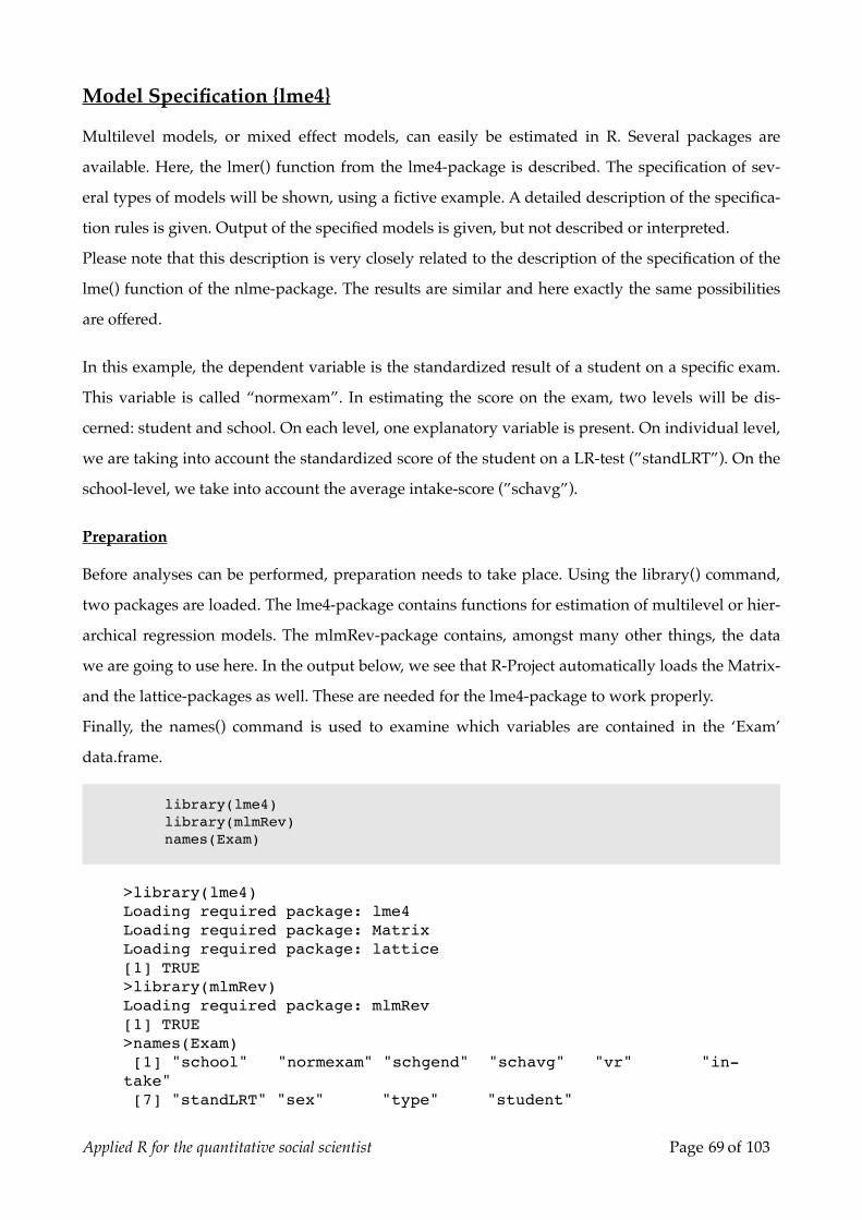
Model Specification {lme4}

Multilevel models, or mixed effect models, can easily be estimated in R. Several packages are

available. Here, the lmer() function from the lme4-package is described. The specification of sev-

eral types of models will be shown, using a fictive example. A detailed description of the specifica-

tion rules is given. Output of the specified models is given, but not described or interpreted.

Please note that this description is very closely related to the description of the specification of the

lme() function of the nlme-package. The results are similar and here exactly the same possibilities

are offered.

In this example, the dependent variable is the standardized result of a student on a specific exam.

This variable is called “normexam”. In estimating the score on the exam, two levels will be dis-

cerned: student and school. On each level, one explanatory variable is present. On individual level,

we are taking into account the standardized score of the student on a LR-test (”standLRT”). On the

school-level, we take into account the average intake-score (”schavg”).

Preparation

Before analyses can be performed, preparation needs to take place. Using the library() command,

two packages are loaded. The lme4-package contains functions for estimation of multilevel or hier-

archical regression models. The mlmRev-package contains, amongst many other things, the data

we are going to use here. In the output below, we see that R-Project automatically loads the Matrix-

and the lattice-packages as well. These are needed for the lme4-package to work properly.

Finally, the names() command is used to examine which variables are contained in the ‘Exam’

data.frame.

library(lme4)library(mlmRev)names(Exam)

>library(lme4)Loading required package: lme4Loading required package: MatrixLoading required package: lattice[1] TRUE>library(mlmRev)Loading required package: mlmRev[1] TRUE>names(Exam) [1] "school" "normexam" "schgend" "schavg" "vr" "in-take" [7] "standLRT" "sex" "type" "student"


null-model

The syntax below specifies the most simple multilevel regression model of all: the null-model.

Only the levels are defined. Using the lmer-function, the first level (here: students) do not have to

be specified. It is assumed that the dependent variable (here: normexam) is on the first level (which

it should be).

The model is specified using standard R formulas: First the dependent variable is given, followed

by a tilde ( ~ ). The ~ should be read as: “follows”, or: “is defined by”. Next, the predictors are de-

fined. In this case, only the intercept is defined by entering a ‘1′. Next, the random elements are

specified between brackets ( ). Inside these brackets we specify the random predictors, followed by

a vertical stripe ( | ), after which the group-level is specified.

After the model specification, several parameters can be given to the model. Here, we specify the

data that should be used by data=Exam. Another often used parameter indicates the estimation

method. If left unspecified, restricted maximum likelihood (REML) is used. Another option would

be: method=”ML”, which calls for full maximum likelihood estimation. All this leads to the follow-

ing model specification:

lmer(normexam ~ 1 + (1 | school), data=Exam)

This leads to the following output:

> lmer(normexam ~ 1 + (1 | school), data=Exam)Linear mixed-effects model fit by REMLFormula: normexam ~ 1 + (1 | school) Data: Exam AIC BIC logLik MLdeviance REMLdeviance 11019 11031 -5507 11011 11015Random effects: Groups Name Variance Std.Dev. school (Intercept) 0.17160 0.41425 Residual 0.84776 0.92074number of obs: 4059, groups: school, 65

Fixed effects: Estimate Std. Error t value(Intercept) -0.01325 0.05405 -0.2452


Random intercept, fixed predictor on individual level

For the next model, we add a predictor to the individual level. We do this, by replacing the ‘1′ of

the previous model by the predictor (here: standLRT). An intercept is always assumed, so it is still

estimated here. It only needs to be specified when no other predictors are specified. Since we don’t

want the effect of the predictor to vary between groups, the specification of the random part of the

model remains identical to the previous model. The same data is used, so we specify data=Exam

again.

lmer(normexam ~ standLRT + (1 | school), data=Exam)

> lmer(normexam ~ standLRT + (1 | school), data=Exam)Linear mixed-effects model fit by REMLFormula: normexam ~ standLRT + (1 | school) Data: Exam AIC BIC logLik MLdeviance REMLdeviance 9375 9394 -4684 9357 9369Random effects: Groups Name Variance Std.Dev. school (Intercept) 0.093839 0.30633 Residual 0.565865 0.75224number of obs: 4059, groups: school, 65

Fixed effects: Estimate Std. Error t value(Intercept) 0.002323 0.040354 0.06standLRT 0.563307 0.012468 45.18

Correlation of Fixed Effects: (Intr)standLRT 0.008

Random intercept, random slope

The next model that will be specified, is a model with a random intercept on individual level and a

predictor that is allowed to vary between groups. In other words, the effect of doing homework on

the score on a math-test varies between schools. In order to estimate this model, the ‘1′ that indi-

cates the intercept in the random part of the model specification is replaced by the variable of

which we want the effect to vary between the groups.

lmer(normexam ~ standLRT + (standLRT | school), data=Exam, method=”ML”)


> lmer(normexam ~ standLRT + (standLRT | school), data=Exam, method="ML")Linear mixed-effects model fit by maximum likelihoodFormula: normexam ~ standLRT + (standLRT | school) Data: Exam AIC BIC logLik MLdeviance REMLdeviance 9327 9358 -4658 9317 9328Random effects: Groups Name Variance Std.Dev. Corr school (Intercept) 0.090406 0.30068 standLRT 0.014548 0.12062 0.497 Residual 0.553656 0.74408number of obs: 4059, groups: school, 65

Fixed effects: Estimate Std. Error t value(Intercept) -0.01151 0.03978 -0.289standLRT 0.55673 0.01994 27.917

Correlation of Fixed Effects: (Intr)standLRT 0.365

Random intercept, individual and group level predictor

It is possible to enter variables on group level as well. Here, we will add a predictor that indicates

the size of the school. The lmer-function needs this variable to be of the same length as variables on

individual length. In other words: for every unit on the lowest level, the variable indicating the

group level value (here: the average score on the intake-test for every school) should have a value.

For this example, this implies that all respondents that attend the same school, have the same

value on the variable “schavg”. We enter this variable to the model in the same way as individual

level variables, leading to the following syntax:

lmer(normexam ~ standLRT + schavg + (1 + standLRT | school), data=Exam)


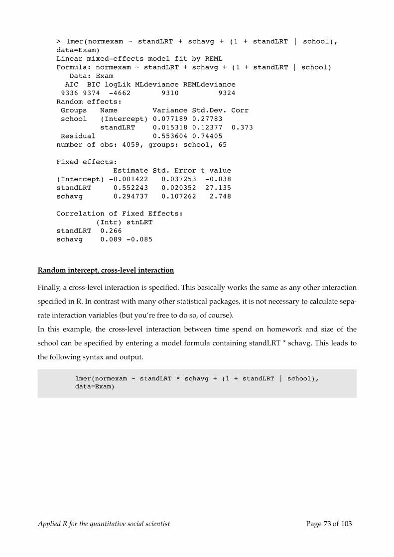
> lmer(normexam ~ standLRT + schavg + (1 + standLRT | school), data=Exam)Linear mixed-effects model fit by REMLFormula: normexam ~ standLRT + schavg + (1 + standLRT | school) Data: Exam AIC BIC logLik MLdeviance REMLdeviance 9336 9374 -4662 9310 9324Random effects: Groups Name Variance Std.Dev. Corr school (Intercept) 0.077189 0.27783 standLRT 0.015318 0.12377 0.373 Residual 0.553604 0.74405number of obs: 4059, groups: school, 65

Fixed effects: Estimate Std. Error t value(Intercept) -0.001422 0.037253 -0.038standLRT 0.552243 0.020352 27.135schavg 0.294737 0.107262 2.748

Correlation of Fixed Effects: (Intr) stnLRTstandLRT 0.266schavg 0.089 -0.085

Random intercept, cross-level interaction

Finally, a cross-level interaction is specified. This basically works the same as any other interaction

specified in R. In contrast with many other statistical packages, it is not necessary to calculate sepa-

rate interaction variables (but you’re free to do so, of course).

In this example, the cross-level interaction between time spend on homework and size of the

school can be specified by entering a model formula containing standLRT * schavg. This leads to

the following syntax and output.

lmer(normexam ~ standLRT * schavg + (1 + standLRT | school), data=Exam)


> lmer(normexam ~ standLRT * schavg + (1 + standLRT | school), data=Exam)Linear mixed-effects model fit by REMLFormula: normexam ~ standLRT * schavg + (1 + standLRT | school) Data: Exam AIC BIC logLik MLdeviance REMLdeviance 9334 9379 -4660 9303 9320Random effects: Groups Name Variance Std.Dev. Corr school (Intercept) 0.076326 0.27627 standLRT 0.012240 0.11064 0.357 Residual 0.553780 0.74416number of obs: 4059, groups: school, 65

Fixed effects: Estimate Std. Error t value(Intercept) -0.00709 0.03713 -0.191standLRT 0.55794 0.01915 29.134schavg 0.37341 0.11094 3.366standLRT:schavg 0.16182 0.05773 2.803

Correlation of Fixed Effects: (Intr) stnLRT schavgstandLRT 0.236schavg 0.070 -0.064stndLRT:sch -0.065 0.087 0.252

Model specification {nlme}

Multilevel models, or mixed effect models, can easily be estimated in R. Several packages are

available. Here, the lme() function from the nlme-package is described. The specification of several

types of models will be shown, using a fictive example. A detailed description of the specification

rules is given. Output of the specified models is given, but not described or interpreted.

Please note that this description is very closely related to the description of the specification of the

lmer() function of the lme4-package. The results are similar and here exactly the same possibilities

are offered.

In this example, the dependent variable is the standardized result of a student on a specific exam.

This variable is called “normexam”. In estimating the score on the exam, two levels will be dis-

cerned: student and school. On each level, one explanatory variable is present. On individual level,

we are taking into account the standardized score of the student on a LR-test (”standLRT”). On the

school-level, we take into account the average intake-score (”schavg”).


Preparation

Before analyses can be performed, preparation needs to take place. Using the library() command,

two packages are loaded. The nlme-package contains functions for estimation of multilevel or hi-

erarchical regression models. The mlmRev-package contains, amongst many other things, the data

we are going to use here. In the output below, we see that R-Project automatically loads the Matrix-

and the lattice-packages as well. These are needed for the mlmRev-package to work properly.

Finally, the names() command is used to examine which variables are contained in the ‘Exam’

data.frame.

require(nlme)require(mlmRev)names(Exam)

Note that in the output below, R-Project notifies us that the objects ‘Oxboys’ and ‘bdf’ are masked

when the mlmRev-package is loaded. This is simply caused by the fact, that objects with similar

names were already loaded as part of the nlme-package. When we know that these objects contain

exactly the same data or functions, there is nothing to worry about. If we don’t know that or if we

do indeed have knowledge of differences, we should be careful in which order the packages are

loaded. Since we don’t need those here, there is no need to further investigate that.

> require(nlme)Loading required package: nlme[1] TRUE> require(mlmRev)Loading required package: mlmRevLoading required package: lme4Loading required package: MatrixLoading required package: lattice

Attaching package: 'mlmRev'

The following object(s) are masked from package:nlme :

Oxboys, bdf

[1] TRUE> names(Exam) [1] "school" "normexam" "schgend" "schavg" "vr" "in-take" [7] "standLRT" "sex" "type" "student"


Null-model

The syntax below specifies the most simple multilevel regression model of all: the null-model.

Only the levels are defined. Using the lme-function, the first level (here: students) do not have to

be specified. It is assumed that the dependent variable (here: normexam) is on the first level (which

it should be).

The model is specified using two standard R formulas, respectively for the fixed part and for the

random part, in indicating the different levels as well. The fixed and the random formulas are pre-

ceded by respectively ‘fixed =’ and ‘random =’. In the formula for the fixed part, first the depend-

ent variable is given, followed by a tilde ( ~ ). The ~ should be read as: “follows”, or: “is defined

by”. Next, the predictors are defined. In this case, only the intercept is defined by entering a ‘1′.

The formula for the random part is given, stating with a tilde (~). The dependent variable is not

given here. Then the random variables are given, followed by a vertical stripe ( | ), after which the

group-level is specified.

After the model specification, several parameters can be given to the model. Here, we specify the

data that should be used by data=Exam. Another often used parameter indicates the estimation

method. If left unspecified, restricted maximum likelihood (REML) is used. Another option would

be: method=”ML”, which calls for full maximum likelihood estimation. All this leads to the follow-

ing model specification:

lme(fixed = normexam ~ 1,data = Exam,random = ~ 1 | school)

This leads to the following output:


> lme(fixed = normexam ~ 1,+ data = Exam,+ random = ~ 1 | school)Linear mixed-effects model fit by REML Data: Exam Log-restricted-likelihood: -5507.327 Fixed: normexam ~ 1(Intercept)-0.01325213

Random effects: Formula: ~1 | school (Intercept) ResidualStdDev: 0.4142457 0.9207376

Number of Observations: 4059Number of Groups: 65

Random intercept, fixed predictor in individual level

For the next model, we add a predictor to the individual level. We do this, by replacing the ‘1′ in

the formula for the fixed part of the previous model by the predictor (here: standLRT). An intercept

is always assumed, so it is still estimated here. It only needs to be specified when no other predic-

tors are specified. Since we don’t want the effect of the predictor to vary between groups, the

specification of the random part of the model remains identical to the previous model. The same

data is used, so we specify data=Exam again.

lme(fixed = normexam ~ standLRT,data = Exam,random = ~ 1 | school)

> lme(fixed = normexam ~ standLRT,+ data = Exam,+ random = ~ 1 | school)Linear mixed-effects model fit by REML Data: Exam Log-restricted-likelihood: -4684.383 Fixed: normexam ~ standLRT(Intercept) standLRT0.002322823 0.563306914




Random intercept, random slope

The next model that will be specified, is a model with a random intercept on individual level and a

predictor that is allowed to vary between groups. In other words, the effect of doing homework on

the score on a math-test varies between schools. In order to estimate this model, the ‘1′ that indi-

cates the intercept in the random part of the model specification is replaced by the variable of

which we want the effect to vary between the groups.

lme(fixed = normexam ~ standLRT,data = Exam,random = ~ standLRT | school)

> lme(fixed = normexam ~ standLRT,+ data = Exam,+ random = ~ standLRT | school)Linear mixed-effects model fit by REML Data: Exam Log-restricted-likelihood: -4663.8 Fixed: normexam ~ standLRT(Intercept) standLRT-0.01164834 0.55653379

Random effects: Formula: ~standLRT | school Structure: General positive-definite, Log-Cholesky parametriza-tion StdDev Corr(Intercept) 0.3034980 (Intr)standLRT 0.1223499 0.494Residual 0.7440699


Random intercept, individual and group level predictor

It is possible to enter variables on group level as well. Here, we will add a predictor that indicates

the size of the school. The lme()-function needs this variable to be of the same length as variables

on individual length. In other words: for every unit on the lowest level, the variable indicating the

group level value (here: the average score on the intake-test for every school) should have a value.

For this example, this implies that all respondents that attend the same school, have the same

value on the variable “schavg”. We enter this variable to the model in the same way as individual

level variables, leading to the following syntax:


lme(fixed = normexam ~ standLRT + schavg,data = Exam,random = ~ standLRT | school)

> lme(fixed = normexam ~ standLRT + schavg,+ data = Exam,+ random = ~ standLRT | school)Linear mixed-effects model fit by REML Data: Exam Log-restricted-likelihood: -4661.943 Fixed: normexam ~ standLRT + schavg (Intercept) standLRT schavg-0.001422435 0.552241377 0.294758810



Random intercept, cross-level interaction

Finally, a cross-level interaction is specified. This basically works the same as any other interaction

specified in R. In contrast with many other statistical packages, it is not necessary to calculate sepa-

rate interaction variables (but you’re free to do so, of course).

In this example, the cross-level interaction between time spend on homework and size of the

school can be specified by entering a model formula containing standLRT * schavg. This leads to

the following syntax and output.

lme(fixed = normexam ~ standLRT * schavg,data = Exam,random = ~ standLRT | school)


> lme(fixed = normexam ~ standLRT * schavg,+ data = Exam,+ random = ~ standLRT | school)Linear mixed-effects model fit by REML Data: Exam Log-restricted-likelihood: -4660.194 Fixed: normexam ~ standLRT * schavg (Intercept) standLRT schavg standLRT:schavg -0.007091769 0.557943270 0.373396511 0.161829150



Generalized Multilevel Models {lme4}

Although all introductions on regression seem to be based on the assumption of data that is dis-

tributed normally, in practice this is not always the case. Many other types of distributions exist. To

name a few: normal distribution, binomial distribution, poisson, gaussian and so on. The lmer()-

function in the lme4-package can easily estimate models based on these distributions. This is done

by adding the ‘family’-argument to the command syntax, thereby specifying that not a linear mul-

tilevel model needs to be estimated, but a generalized linear model.

Logistic Multilevel Regression

Let us say, we want to estimate the chance for success on a test a student in a specific school has.

Therefor, we can use the Exam data-set in the mlmRev-package. This contains the standardized

scores on a test. Here, we’ll define success on the test as having a standardized score of 0 or larger.

This is recoded to a 0-1 variable below, using the ifelse() function. Using summary() the process of

recoding is checked. The needed packages are loaded as well, using the library() function.

library(lme4)library(mlmRev)names(Exam)

Exam$success <- ifelse(Exam$normexam >= 0,1,0)summary(Exam$normexam)summary(Exam$success)


> library(lme4)Loading required package: MatrixLoading required package: lattice> library(mlmRev)> names(Exam) [1] "school" "normexam" "schgend" "schavg" "vr" "in-take" [7] "standLRT" "sex" "type" "student">> Exam$success <- ifelse(Exam$normexam >= 0,1,0)> summary(Exam$normexam) Min. 1st Qu. Median Mean 3rd Qu. Max.-3.6660000 -0.6995000 0.0043220 -0.0001138 0.6788000 3.6660000> summary(Exam$success) Min. 1st Qu. Median Mean 3rd Qu. Max. 0.0000 0.0000 1.0000 0.5122 1.0000 1.0000

In order to be able to properly use the so created binary ’success’ variable, a logistic regression

model needs to be estimated. This is done by specifying binomial family, using the logit as a link-

function, using “family = binomial(link = “logit”)”. The rest of the specification is exactly the same

as a normal linear multilevel regression model using the lmer() function.

lmer(success~ schavg + (1|school), data=Exam, family=binomial(link = “logit”))


> lmer(success~ schavg + (1|school),+ data=Exam,+ family=binomial(link = "logit"))Generalized linear mixed model fit using LaplaceFormula: success ~ schavg + (1 | school) Data: Exam Family: binomial(logit link) AIC BIC logLik deviance 5323 5342 -2658 5317Random effects: Groups Name Variance Std.Dev. school (Intercept) 0.23113 0.48076number of obs: 4059, groups: school, 65

Estimated scale (compare to 1 ) 0.9909287

Fixed effects: Estimate Std. Error z value Pr(>|z|)(Intercept) 0.08605 0.07009 1.228 0.220schavg 1.60548 0.21374 7.511 5.86e-14 ***---Signif. codes: 0 '***' 0.001 '**' 0.01 '*' 0.05 '.' 0.1 ' ' 1

Correlation of Fixed Effects: (Intr)schavg 0.072

Extractor Functions

Unlike most statistical software packages, R often stores the results of an analysis in an object. The

advantage of this is that while not all output is shown in the screen ad once, it is neither necessary

to estimate the statistical model again if different output is required.

This paragraph will show the kind of data that is stored in a multilevel model estimated by R-

Project and introduce some functions that make use of this data.

Inside the model

Let’s first estimate a simple multilevel model, using the nlme-package. For this paragraph we will

use a model we estimated earlier: the education model with a random intercept and a random

slope. This time though, we will assign it to an object that we call model.01. It is estimated as fol-

lows:

require(nlme)require(mlmRev)

model.01 <- lme(fixed = normexam ~ standLRT, data = Exam,random = ~ standLRT | school)


Basically, this results in no output at all, although the activation of the packages creates a little out-

put. Basic results can be obtained by simply calling the object:

model.01

> model.01Linear mixed-effects model fit by REML Data: Exam Log-restricted-likelihood: -4663.8 Fixed: normexam ~ standLRT(Intercept) standLRT-0.01164834 0.55653379



This gives a first impression of the estimated model. But, there is more. To obtain an idea of the

elements that are actually stored inside the model, we use the names() functions, that gives us the

names of all the elements of the model.

names(model.01)model.01$methodmodel.01$logLik

The output below shows that our model.01 contains seventeen elements. For reasons of space, only

some will be described. ‘Contrasts’ contains information on the way categorical variables were

handled, ‘coefficients’ contains the model-parameters, in ‘call’ the model formula is stored and in

‘data’ even the original data is stored.

> names(model.01) [1] "modelStruct" "dims" "contrasts" "coefficients" [5] "varFix" "sigma" "apVar" "logLik" [9] "numIter" "groups" "call" "terms"[13] "method" "fitted" "residuals" "fixDF"[17] "data"> model.01$method[1] "REML"> model.01$logLik[1] -4663.8


In the syntax above two specific elements of the model were requested: the estimation method and

the loglikelihood. This is done by sub-setting the model using the $-sign after which the desired

element is placed. The output tells us that model.01 was estimated using Restricted Maximum

Likelihood and that the loglikelihood is -4663.8 large.

Summary

All the information we could possibly want is stored inside the models, as we have seen. In order

to receive synoptic results, many functions exist to extract some of the elements from the model

and present them clearly. The most basic of these extractor-functions is probably summary():

summary(model.01)

> summary(model.01)Linear mixed-effects model fit by REML Data: Exam AIC BIC logLik 9339.6 9377.45 -4663.8


Fixed effects: normexam ~ standLRT Value Std.Error DF t-value p-value(Intercept) -0.0116483 0.04010986 3993 -0.290411 0.7715standLRT 0.5565338 0.02011497 3993 27.667639 0.0000 Correlation: (Intr)standLRT 0.365

Standardized Within-Group Residuals: Min Q1 Med Q3 Max-3.8323045 -0.6316837 0.0339390 0.6834319 3.4562632



Anova

The last extractor function that will be shown here is anova. This is a very general function that can

be used for a great variety of models. When it is applied to a multilevel model, it results in a basic

test for statistical significance of the model-parameters, as is showed below.

anova(model.01)

model.02 <- lme(fixed = normexam ~ standLRT, data = Exam,random = ~ 1 | school)

anova(model.02,model.01)

In the syntax above an additional model is estimated that is very similar to our model.01, but does

not have a random slope. It is stored in the object model.02. This is done to show that it is possible

to test whether the random slope model fits better to the data than the fixed slope model. The out-

put below shows that this is indeed the case.

> anova(model.01) numDF denDF F-value p-value(Intercept) 1 3993 124.3969 <.0001standLRT 1 3993 765.4983 <.0001>> model.02 <- lme(fixed = normexam ~ standLRT, data = Exam,+ random = ~ 1 | school)>> anova(model.02,model.01) Model df AIC BIC logLik Test L.Ratiomodel.02 1 4 9376.765 9401.998 -4684.383model.01 2 6 9339.600 9377.450 -4663.800 1 vs 2 41.16494 p-valuemodel.02model.01 <.0001

Helper Functions

Several functions already present in R-Project are very useful when analyzing multilevel models or

when preparing data to do so. Three of these helper functions will be described: aggregating data,

the behavior of the plot() function when applied to a multilevel model and finally setting contrasts

for categorical functions. Note that none of these functions are related to multilevel analysis only.

Aggregate

We will continue to work with the Exam-dataset that is made available through the mlmRev-

package. In the syntax below we load that package and use the names() function to see what vari-


ables are available in the Exam data-set. One of the variables on individual level is the normexam-

variable. Let’s say we want to aggregate this variable to the school-level, so that the new variable

represents for each student the level of the exam-score at school level.

library(mlmRev)names(Exam)

meansch <- tapply(Exam$normexam, Exam$school, mean)meansch[1:10]Exam$meanexam <- meansch[Exam$school]names(Exam)

Using tapply(), we create a table of the normexam-variable by school, calculating the mean for

each school. The result of this is stored in the meansch-variable. This variable now contains 65 val-

ues representing the mean score on the normexam-variable for each school. The first ten of these

values is shown. This meansch-variable is only a temporary helping variable. Then we create a

new variable in the Exam-data.frame called meanexam as well (this can be any name you want, as

long as it does not already exist in the data.frame).

We give the correct value on this new variable to each respondent, by indexing the meansch by the

school-index stored in the Exam-data.frame. When we look at the names of the Exam data.frame

now, we see that our new variable is added to it.

> library(mlmRev)> names(Exam) [1] "school" "normexam" "schgend" "schavg" "vr" [6] "intake" "standLRT" "sex" "type" "student"[11] "meansch">> meansch <- tapply(Exam$normexam, Exam$school, mean)> meansch[1:10] 1 2 3 4 5 0.501209573 0.783102291 0.855444696 0.073628516 0.403608663 6 7 8 9 10 0.944579967 0.391500023 -0.048192541 -0.435682141 -0.269390664> Exam$meanexam <- meansch[Exam$school]> names(Exam) [1] “school” “normexam” “schgend” “schavg” “vr” [6] “intake” “standLRT” “sex” “type” “student”[11] “meansch” “meanexam”


plot (multilevel.model)

R-Project has many generic functions, that behave differently when different data is provided to it.

A good example of this is the plot()-function. We have already seen how this function can be used

to plot simple data. When it is used to plot an estimated multilevel model, it will extract the re-

siduals from it and the result is a plot of the standardized residuals.

library(nlme)

model.01 <- lme(fixed = normexam ~ standLRT,data = Exam,random = ~ 1 | school)

plot(model.01, main="Residual plot of model.01")

In the syntax above, this is illustrated using a basic multilevel

model, based on the Exam-data. First, the nlme-package is

loaded, which results in a few warning messages (not shown

here) that indicate that some data-sets are loaded twice (they

were already loaded with the mlmRev-package). We assign

the estimated model, that has a random intercept by schools

and a predictor on the first (individual) level, to an object we

have called ‘model.01′.

When this is plotted, we see that the residuals are distributed

quite homoscedastically. The layout of the plot-window is quite different from what we have seen

before. The reason for this is that here the lattice-package for advanced graphics is automatically

used.

Contrasts

When using categorical data in regression analyses (amongst other types of analysis), it is needed

to code dummy-variables or contrasts. This can be done manually of course, as needs to be done in

some other statistical packages, but in R-Project this is done automatically. The ‘vr’-variable in the

Exam-dataset represents “Student level Verbal Reasoning (VR) score band at intake - a factor. Lev-

els are bottom 25%, mid 50%, and top 25%.” (quote from the description of the dataset, found by

using ?Exam). In the syntax below, a summary of this variable is asked for, resulting in a confirma-

tion that this variable contains three categories indeed.

Then, a basic model is estimated using the ‘vr’-variable and assigned to an object called model.02

(it is a random intercept model at school level containing two variables on individual level (’vr’


and ’standLRT’) and one variable on second level (’schavg’). The summary of that model shows

that it is the first category, representing the lowest Verbal Reasoning score band, that is used as ref-

erence category in the analyses.

summary(Exam$vr)

model.02 <- lme(fixed = normexam ~ vr + standLRT + schavg,data = Exam,random = ~ 1 | school)

summary(model.02)

> summary(Exam$vr)bottom 25% mid 50% top 25% 640 2263 1156>> model.02 <- lme(fixed = normexam ~ vr + standLRT + schavg,+ data = Exam,+ random = ~ 1 | school)>> summary(model.02)Linear mixed-effects model fit by REML Data: Exam AIC BIC logLik 9379.377 9423.53 -4682.689


Fixed effects: normexam ~ vr + standLRT + schavg Value Std.Error DF t-value p-value(Intercept) 0.0714396 0.16717547 3993 0.42733 0.6692vrmid 50% -0.0834973 0.16341508 61 -0.51095 0.6112vrtop 25% -0.0537963 0.27433650 61 -0.19610 0.8452standLRT 0.5594779 0.01253795 3993 44.62276 0.0000schavg 0.4007454 0.28016707 61 1.43038 0.1577 Correlation: (Intr) vrm50% vrt25% stnLRTvrmid 50% -0.946vrtop 25% -0.945 0.886standLRT 0.000 0.000 0.000schavg 0.863 -0.794 -0.914 -0.045




Should we want to change that, we need to use the contrast() function. When used on the ‘vr’-

variable, it makes clear why the first category of the variable is used as reference: in the resulting

matrix it is the only category without a ‘1′ on one of the columns.

To change this, we have two options at hand. First we use the contr.treatment()-function. We want

the third category used as reference now. So, we specify that the contrasts should be treated in such

a way that the categories are based on the levels of the ‘vr’-variable and that the base, or reference,

should be the third. The result of the contr.treatment()-function looks exactly like the result of the

contrasts()-function (except for a different reference category obviously). To change the used refer-

ence in an analysis, the result of the contr.treatment()-function should be assigned to the con-

trast(Exam$vr). The old contrasts -settings are replaced by the new ones in that way.

Instead of using the contr.treatment() function we can simply create a matrix ourselves and use this

to change the contrasts. This is done below in order to make clear what is actually happening

when the contr.treatment()-function is used. First the matrix is shown, then it is assigned to the

contrasts of the ‘vr’-variable. Now we have chosen the middle category to be the reference. Al-

though this works perfectly, the draw-back of this procedure is that the value-labels of the variable

are lost, while these are maintained when contr.treatment() is used.

contrasts(Exam$vr)contrasts(Exam$vr) <- contr.treatment(levels(Exam$vr), base=3)contrasts(Exam$vr)matrix(data=c(1,0,0,0,0,1), nrow = 3, ncol = 2, byrow=FALSE)contrasts(Exam$vr) <- matrix(data=c(1,0,0,0,0,1), nrow = 3, ncol = 2, byrow=FALSE)contrasts(Exam$vr)


> contrasts(Exam$vr) mid 50% top 25%bottom 25% 0 0mid 50% 1 0top 25% 0 1> contr.treatment(levels(Exam$vr), base=3) bottom 25% mid 50%bottom 25% 1 0mid 50% 0 1top 25% 0 0> contrasts(Exam$vr) <- contr.treatment(levels(Exam$vr), base=3)> contrasts(Exam$vr) bottom 25% mid 50%bottom 25% 1 0mid 50% 0 1top 25% 0 0> matrix(data=c(1,0,0,0,0,1), nrow = 3, ncol = 2, byrow=FALSE) [,1] [,2][1,] 1 0[2,] 0 0[3,] 0 1> contrasts(Exam$vr) <- matrix(data=c(1,0,0,0,0,1), nrow = 3, ncol = 2, byrow=FALSE)> contrasts(Exam$vr) [,1] [,2]bottom 25% 1 0mid 50% 0 0top 25% 0 1>

Finally, using the new contrasts-settings of the ‘vr’-variable, the same model is estimated again. In

the output below, we see that indeed the value labels are gone now (because of using a basic ma-

trix to set the contrasts) and that the middle category is used as reference, although the categories

are now referred to as ‘1′ and ‘2′ which might lead to confusing interpretations.

model.03 <- lme(fixed = normexam ~ vr + standLRT + schavg,data = Exam,random = ~ 1 | school)

summary(model.03)


> model.03 <- lme(fixed = normexam ~ vr + standLRT + schavg,+ data = Exam,+ random = ~ 1 | school)>> summary(model.03)Linear mixed-effects model fit by REML Data: Exam AIC BIC logLik 9379.377 9423.53 -4682.689


Fixed effects: normexam ~ vr + standLRT + schavg Value Std.Error DF t-value p-value(Intercept) -0.0120577 0.05427674 3993 -0.22215 0.8242vr1 0.0834973 0.16341508 61 0.51095 0.6112vr2 0.0297010 0.15018792 61 0.19776 0.8439standLRT 0.5594779 0.01253795 3993 44.62276 0.0000schavg 0.4007454 0.28016707 61 1.43038 0.1577 Correlation: (Intr) vr1 vr2 stnLRTvr1 -0.096vr2 -0.551 -0.530standLRT 0.000 0.000 0.000schavg 0.267 0.794 -0.806 -0.045



Plotting Multilevel models

Plotting the results of a multilevel analysis can be quite complicated while using R. Using only the

basic packages, as well as the multilevel packages (nlme and lme4) there are no functions readily

available for this task. So, this is a good point in this manual to put some of our programming

skills to use. This makes exactly clear how the results of a multilevel analysis are stored in R as

well. For more information on programming functions in R, see the section on programming (not

yet available).

In order to be able to plot a multilevel model, we first need such a model. We will estimate a model

here, which we have seen before. We want to estimate the effect that a standardized test at school-

entry has on a specific exam students made. Students are, of course, nested withing shools, which

is taken into account in our analysis, as well as the average score in the intake test for each of the


schools. The effects the test at entry of the school has on the test result is allowed to vary by school.

In other words: we are estimating a random intercept model with a random slope.

In order to do so, we have to load the nlme package, as well as the mlmREV-package, which con-

tains the data we will use. Then, for technical reasons, we have to get rid of the lme4-package. This

is done by using the detach() function. This is what is done in the syntax below.

library(nlme)library(mlmRev)detach(”packages:lme4″)

model.01 <- lme(fixed = normexam ~ standLRT + schavg,data = Exam,random = ~ standLRT | school)

summary(model.01)

The requested output of the model.01 results in:

> summary(model.01)Linear mixed-effects model fit by REML Data: Exam AIC BIC logLik 9337.885 9382.04 -4661.943


Fixed effects: normexam ~ standLRT + schavg Value Std.Error DF t-value p-value(Intercept) -0.0014224 0.03725472 3993 -0.038181 0.9695standLRT 0.5522414 0.02035359 3993 27.132378 0.0000schavg 0.2947588 0.10726821 63 2.747867 0.0078 Correlation: (Intr) stnLRTstandLRT 0.266schavg 0.089 -0.085




Probably the best way to visualize this model is to create a plot of the relationship on individual

level between the score a student had on an standardized intake test (standLRT) and the result on

an specific exam (normexam). We want these relationship to be shown for each school specifically.

To do this, several steps are needed:

• A plot region has to be set

• Coefficients for each school need to be extracted from the model

• The minimum and maximum value on the x-axis for each school need to be extracted

• Based on the model, the data actually needs to be plotted

Each of the steps shall be described explicitly below. Since many steps need to be performed, they

will be gathered in a function, which we’ll call visualize.lme(). It will have three parameters: the

model we want to use, the predictor and the group-variable that will be taken into account.

visualize.lme <- function (model, coefficient, group, ...){r <- ranef(model)f <- fixef(model)

effects <- data.frame(r[,1]+f[1], r[,2]+f[2])

number.lines <- nrow(effects)

Above, the first row defines the function visualize.lme(), an arbitrary name we chose ourselves.

Between the brackets, four elements are placed. The three needed elements described above are

named ‘model’, ‘coefficient’, and ‘group’. The fourth element ( … ) means that any other element

can be added. These elements will be transfered to the plot() function that will be used to set the

graphics device.

Then, four variables are created within the function, to which data from the model is extracted.

First, ranef() extracts the random coefficients from the model, while fixef() does the same for the

fixed elements.

The effects variable is created next. This will be a data.frame that contains information on the inter-

cepts and the slopes that will be plotted. The number.lines variable contains the number of rows in

the effects data.frame, that is equal to the number of groups in the model.


predictor.min <- tapply(model$data[[coefficient]], model$data[[group]], min)predictor.max <- tapply(model$data[[coefficient]], model$data[[group]], max)

outcome.min <- min(predict(model))outcome.max <- max(predict(model))

Before the plotting area can be set up, we will need four coordinates. This is done above. First, the

minimum and maximum value of the predictor is gathered. Next, the minimum and maximum of

the predicted values are determined, using predict(). The predict() function takes the data from the

model specified and uses the original data and the estimated model formula (which are stored in-

side) and returns a vector of predicted values on the outcome-variable. Using min() and max(), the

minimum and maximum values are obtained.

plot (c(min(predictor.min), max(predictor.max)), c(outcome.min,outcome.max), type=”n”, …)

for (i in 1:number.lines){expression <- function(x) {effects[i,1] + (effects[i,2] * x) }curve(expression, from=predictor.min[i], to=predictor.max[i], add=TRUE)}}

Finally, the plot is created above. First, the area in which to plot is set up. Using the four coordi-

nates obtained before, a plot is created in such a way, that the lines the will be plotted next will fit

in exactly. Specifying type=”n” results in setting up a plotting region on a graphics device, without

an actual plot being made. Only the axes that are created can be seen. The … parameter in the

specification of the plot() function transfers all the additional parameters that are given to the

visualize.lme() we’re creating to the plot()-function that is used here. We can use it to give proper

names to both axes, as well as to set a title for the plot.

Then, a loop is created using for(). For each of the groups, a line will be plotted. In order to do so, a

function is created based on the intercept and the slopes extracted earlier. Then, this created func-

tion (called ‘expression’) is entered into the curve()-function. This curve()-function draws a graph

based on a function (for instance, the one we just created) from a starting point to an end-point that

both are specified. This process is repeated for every group in the model, resulting in a basic graph

based on our multilevel, random intercept and random slope regression model.


The complete syntax of this function will be shown below, as well as the result when used on the

model we estimated at the start of this paragraph. This full syntax can be entered into R and then

used for plotting other multilevel models. In future versions of this manual, the Trellis-graphics

system, contained in the Lattice-package, will be introduced. Using that advanced graphics pack-

age, plotting of multilevel models is much more convenient and sophisticated.

visualize.lme <- function (model, coefficient, group, ...){r <- ranef(model)f <- fixef(model)

effects <- data.frame(r[,1]+f[1], r[,2]+f[2])

number.lines <- nrow(effects)

predictor.min <- tapply(model$data[[coefficient]], model$data[[group]], min)predictor.max <- tapply(model$data[[coefficient]], model$data[[group]], max)

outcome.min <- min(predict(model))outcome.max <- max(predict(model))

plot (c(min(predictor.min),max(predictor.max)),c(outcome.min,outcome.max), type="n", ...)

for (i in 1:number.lines){expression <- function(x) {effects[i,1] + (effects[i,2] * x) }curve(expression, from=predictor.min[i], to=predictor.max[i], add=TRUE)}}

visualize.lme(model.01, "standLRT", "school", xlab="Student test at school-entry", ylab="Result on Exam", main="Exam results for 65 schools")



Chapter Five: Books on R-Project


Mixed-Effect Models in S and S-PLUS

Pinheiro, José C., & Bates, Douglas, M. (2000), Mixed-Effects Models in S

and S-PLUS, Springer, New York. ISBN: 0-387-98957-9

Despite the reference to S and S-PLUS in the title of this book, it offers

an excellent guide for the nlme-package in R-Project. Reason for this

is the close resemblance between R and S. The nlme-package, avail-

able in R-Project for estimation of both linear and non-linear multi-

level models, is written and maintained by the authors of this book.

The book is not an introduction to R. Basis knowledge of R-Project (or

S / S-PLUS) is required to get the most out of it, as well as some

knowledge on multilevel theory. Although the book forms a thorough

introduction into multilevel modeling, addressing both some theory, the mathematics and of

course the estimation and specification in R-Project, the learning curve it offers is quite steep. The

authors are not shunned to apply matrix algebra and specify exactly the used estimation proce-

dures.

Not only the specification of basic models is described, but many other subjects are brought up. A

specific grouped-data object is considered, as well as ways to visualize hierarchical data and multi-

level models. Heteroscedasticity, often a violation of assumptions, can be caught in the models eas-

ily, as is described clearly in one of the chapters. Finally, not only linear models are tackled, but

non-linear models as well.

All in all, this book is an excellent addition for those who have prior knowledge of both R-Project

and multilevel analysis. Using real-data examples and by providing tons of output, the authors

accomplish to make clear the necessity of the more complex models and thereby invite the reader

to invest time for the more fundamental aspects of multilevel analysis.


An R and S-PLUS Companion to Applied Regression

Fox, John (2002), An R and S-PLUS Companion to Applied Regression. Sage Publications, London. ISBN:

0-7619-2280-6

For those who have theoretical knowledge on statistics and regres-

sion techniques, and who want to learn to use R-Project to analyze

some data, John Fox wrote just the book.

The introductory chapter shows the most basic aspects of R-Project.

Halfway this chapter the reader finds himself analyzing real data

using regression techniques. The following chapters introduce the

reader to other aspects of the analytical process: reading data into

your statistical program, exploring the data and performing some

bivariate tests. Then, three full chapters are devoted to regression

techniques. While working on practical examples, the reader is in-

troduced to more fundamental aspects of the R-Project software where needed.

The beauty of R is, that anybody can make alterations and additions to it. John Fox did so on many

functions, as well as added some functionality that resemble a SPSS-like usage. For instance, recod-

ing in R-Project is normally done using conditionals. This can lead to a somewhat cumbersome

process, so Fox wrote his own ‘recode’ function, in which values, or ranges of values, can be speci-

fied, as well as output-values. For many people this, and many other functions, will enhance their

usage of R-Project. The drawback of this is that the fundamentals of R usage are lost out of sight.

But then, the book is called ‘companion to applied regression’.

A broad array of analytical techniques is addressed, with a focus on regression. Both linear models

as well as generalized models are described. A full chapter is reserved for diagnostics of the model

fit. Finally, a chapter is devoted to graphically presenting results and the last chapter gives an in-

troduction to programming in R. Although the book ends there, many other statistical techniques

are covered by Fox in web-appendices that are freely available. Among the covered techniques in

these appendices are structural equation modeling, multilevel modeling, and several specific types

of regression, such as: non-parametric, robust, time-series and nonlinear regression.

This pleasantly written book is excellent for those who want to use R-Project as their main statisti-

cal software. Some knowledge on statistics is requires, while all the basics of R-Project are de-


scribed. For the more advanced techniques, web-appendices were made available. Summarizing,

this book is a good introduction, as well a reference. As the title says, it is a fine companion.

Introductory Statistics with R

Dalgaard, Peter (2002), Introductory Statistics with R. Springer, New York. ISBN: 0-387-95475

Peter Dalgaard is associate professor at the Department of Biostatis-

tics at the University of Copenhagen in Denmark, and a member of

the R-Project Core Development team. Also, he is an active partici-

pating and respected member of the R-help mailing-list. Based on

these experiences, he set to write an introductory book on statistics

and R.

The book start with relatively simple subjects, easily working toward

more complex statistical problems. Central techniques that are cov-

ered are analysis of variance and regression. Starting with bivariate

analyses, multivariate analyses of both types are discussed to a high

extent. Several types of linear (regression) models are introduced, cov-

ering polynomial regression, regression without an intercept, interactional model, two-way

ANOVA with replication, and ANCOVA. A separate chapter focusses on logistic regression.

Moreover, in many ways the equivalence or parallels of regression and ANOVA are discussed.

Thereby, a greater understanding of the (differences between) techniques is stimulated.

In the course of the book, the reader is introduced to R by simple examples. The book has a R-

package available for download that contains several data-sets that are used throughout the book.

An appendix in the book describes the data-sets. In contrast with many other books on R, the

package does not contain functions that were written by the author. The benefit of that is, is that

the books only relies on the most basic functions that come with a basic installation of R. When the

book was written, the most recent version of R was 1.5.0. Presently, it is 2.4.1, but all the examples

still work without any problem.

The power of the approach in this book, is that both the statistical techniques are introduced, as

well as it is shown how to perform these tests using R. But, while the book aims to be an introduc-

tion to statistics, it somewhat fails to introduce the techniques thoroughly. Strikingly, the author

does not explain (much) on the interpretation of results. For instance, no guidance is given in the

interpretation of the results of a logistics regression. This cannot be expected to be clear for a nov-


ice in statistics. If a reader does not have any understanding of statistics prior to reading this book,

the book will fail in its’ purpose. To put it differently: the book hovers somewhere in between “In-

troductory Statistics with R” and “Introduction to R, using Statistics”.

Any author makes choices when writing, based on his or her background. Differences occur in the

subjects that are addressed. In this, Peter Dalgaard has made some nice choices, that make to book

pleasantly distinguishing from other introductory books. The cross-over between regression and

ANOVA on the applied level has already been mentioned. Other niceties are a chapter dedicated to

determining the statistical power of tests. To students starting to learn about statistics, this might

be a starting point for discussing the relevancy of statistical significance. Another distinguishing

chapter is a chapter on survival analysis. Not often found in starting books on statistics, this chap-

ter shows that statistics in different contexts are based still on the same principles.

Nevertheless, the book seems ideal for teaching purposes in combination with a book that handles

more fundamental issues of statistics. If used in that way, a powerful combination is at hand. The

lack of guidance in interpretation then is not so much of a problem. A difficulty many students in

statistics have, is transferring their new knowledge on a fundamental level to application. This

book will be of help, mostly because it has an emphasis on application, but explains some of the

more important fundamental issues, from a practical perspective. Thereby, when used with prior

knowledge or an additional book on statistics, it is a wonderful addition to applied statistics and

R-Project.

Data Analysis Using Regression and Multilevel/Hierarchical Models

Gelman, Andrew & Hill, Jennifer (2007). Data analysis using regres-

sion and multilevel/hierarchical models. Cambridge University

Press, Cambridge.

Andrew Gelman is known for his expertise on Bayesian statistics.

Based on that knowledge he wrote a book in multilevel regression

using R and WINbugs. This book aims to be a thorough descrip-

tion of (multilevel) regression techniques, implementation of

these techniques in R and bugs, and a guide on interpreting the

results of your analyses. Shortly put, the books excels on all three

subjects.


Admittedly, this review has been written based on first impressions on the book. But, a sunny day

in the park reading this book (literally) left me to believe that I have some understanding on what

this book is trying to achieve. I bought this book in order to have an overview on fitting multilevel

regression models using R. Starting to read the book, I soon found out that that is indeed what it

has to offer me, but it offers me a lot more. After some introductory chapters, the book starts off

with an introduction to both linear regression as well as introducing the reader to R software, by

showing how to fit linear regression models in R. This is readily expanded to logistic regression

and generalized regression models. All is illustrated lushly with many examples and illustrations.

Before these ‘basic’ regression models are extended to multilevel models, Bayesian statistics are

introduced. Based on simulation techniques, causal inferences, based on regression models, are

made. The multilevel section of the book is set up similarly. First, ‘basic’ multilevel regression

models are introduced. Throughout the book, the lmer function is used. This function is not only

able to fit simple multilevel models, but logistic and generalized models as well. It can even esti-

mate non-nested models. All in all, this forms a thorough introduction to multilevel regression

analysis in itself, but the book continues here as well to introduce the reader to Bayesian statistics.

All above-mentioned models, as well as more complicated models, are fitted using WINbugs as

well. This very flexible method allows the reader to estimate a greater variety of (multilevel) mod-

els. Causal inference on multilevel models, using Bayesian statistics, is described as well. The third

main part of the book elaborates on the skills the reader uses to ‘just’ fitting models. It learns the

reader to really think about what it going on. Topics such as ‘understanding and summarizing the

fitted models’, ’sample size and power calculations’, and most of all ‘model checking and compari-

son’ each receive their own chapter of the book. In this we can see that the authors of this book

aimed higher than just writing instructions on how to let R fit (multilevel) regression models. The

aim of this book, is to teach the reader how to analyze data the proper way. Much attention is paid

to assumptions, testing theory, and interpretation of what you’re doing. To quote the authors: “If

you show something, be prepared to explain it”.

This philosophy seemed to be a guideline for the authors while writing this book, as well as flexi-

bility. The book starts off with some examples of the authors’ own research. These examples return

throughout the book, resulting in some degree of familiarity with the data by the reader. Due to

this, the concepts, models and/or analyses described are certainly more easy to be understood. As

a reader, you start to think along with the author, when a new problem is described. The relative

worth of the techniques, as well as their drawbacks, are made perfectly clear. The use of R soft-


ware, as well as WINbugs, pays of well in the sense that it requires some more effort to master

these programs, but in that process the reader learns to think deeply about what he really want to

do and how it is done properly.

It’s not an easy book, but thanks to the many examples throughout the book it can be fully under-

stood by people with some prior knowledge in regression techniques. All of the examples in the

book can be tried yourself, since the data and syntax are available on the author’s website on the

book. This helps the reader to get some feel for the more difficult subjects of the book. All in all,

this seems to me as a great book for every applied researcher that has basic prior understanding of

regression analysis. Due to its focus on one set of techniques, a great depth of understanding can

be derived from this book.


Documents

Applied R for the quantitative social scientist - Curving Normality