Embed Size (px)
Citation preview

Applied Stochastic Control in High Frequency andAlgorithmic Trading
by
Jason Ricci
A thesis submitted in conformity with the requirementsfor the degree of Doctor of Philosophy
Graduate Department of Statistical SciencesUniversity of Toronto
c© Copyright 2014 by Jason Ricci

Abstract
Applied Stochastic Control in High Frequency and Algorithmic Trading
Jason Ricci
Doctor of Philosophy
Graduate Department of Statistical Sciences
University of Toronto
2014
In this thesis, problems in the realm of high frequency trading and optimal market
making are established and solved in both single asset and multiple asset economies. For
an agent that is averse to holding large inventories for long periods of time, optimal high
frequency trading strategies are derived via stochastic control theory and solving the
corresponding Hamilton-Jacobi-Bellman equations. These strategies are analyzed and it
is shown that both inventory control and accounting for adverse selection play critical
roles in the success of an algorithmic trading strategy.
In the single asset problem, a market maker actively modifies her limit quotes in an
economy with asymmetric information. She attempts to keep her inventory small and
posts her limit orders in the limit order book at a depth that mitigates her adverse
selection risk, while not posting too deep in the book as to generate no trade flow. In
addition to this behaviour, a profit maximizing investor trading in multiple assets also
seeks out statistical arbitrage opportunities and acts aggressively via the submission of
market orders when it is deemed optimal to do so.
Throughout this thesis, numerical and practical considerations are made a priority. Full
scale calibration and estimation methods are given in detail, as well as dimensional
reductions for large scale numerical procedures, where appropriate. The bridge from
abstract mathematical theory to practical real-time implementation is made complete as
an entire chapter is dedicated to applications on real data.
ii

Acknowledgements
First and foremost, I would like to express my deepest gratitude to my thesis advisor,
Sebastian Jaimungal, who has provided an unparallelled level of guidance and support
throughout these past few years. This thesis would not have been possible without his
insight and excellence in the discipline.
I would also like to thank my coauthor, Alvaro Cartea from University College London,
for always being willing to share his ideas and advice during our collaboration.
Furthermore, I am grateful to Jeffrey Rosenthal, Luis Seco, and Balint Virag for taking
the time to be part of my thesis committee and providing valuable input throughout
various stages of my research, as well as Mark Reesor from the University of Western
Ontario for having been my external examiner.
I would also like to thank the graduate administrator of the Department of Statistical
Sciences, Andrea Carter, for her unwavering patience when I had inquiries regarding
administrative matters.
Finally, I gratefully acknowledge the financial support of Bank of Montreal (BMO) Cap-
ital Markets and the Ontario Graduate Scholarship (OGS).
iii

Contents
Table of Contents iv
List of Tables x
List of Figures xiv
1 Introduction 1
1.1 Background . . . . . . . . . . . . . . . . . . . . . . . . . . . . . . . . . . 1
1.2 Previous Literature . . . . . . . . . . . . . . . . . . . . . . . . . . . . . . 3
1.3 Main Results & Outline . . . . . . . . . . . . . . . . . . . . . . . . . . . 5
2 The Market Making Problem 7
2.1 Formal Description of the Problem . . . . . . . . . . . . . . . . . . . . . 8
2.2 The Solution . . . . . . . . . . . . . . . . . . . . . . . . . . . . . . . . . 12
2.3 Features of the Optimal Strategy . . . . . . . . . . . . . . . . . . . . . . 14
2.4 The Inclusion of Market Orders . . . . . . . . . . . . . . . . . . . . . . . 17
3 Market Making in a Single Asset 22
3.1 Introduction . . . . . . . . . . . . . . . . . . . . . . . . . . . . . . . . . . 22
iv

3.2 Arrival of Market Orders and Price Dynamics . . . . . . . . . . . . . . . 25
3.2.1 Price Dynamics . . . . . . . . . . . . . . . . . . . . . . . . . . . . 25
3.2.2 Self-Exciting Incoming Market Order Dynamics . . . . . . . . . . 26
3.3 Limit Quote Arrival Dynamics and Fill Rates . . . . . . . . . . . . . . . 29
3.4 Short Term Alpha Dynamics: Directional Strategies and Adverse Selection 33
3.5 The HFT’s Optimization Problem . . . . . . . . . . . . . . . . . . . . . . 34
3.5.1 Formulation of the HF Trading Problem . . . . . . . . . . . . . . 35
3.5.2 The Feedback Control of the Optimal Trading Strategy . . . . . . 37
3.5.3 The Asymptotic Solution of the Optimal Trading Strategy . . . . 39
3.6 HF Market Making, Short Term Alpha, and Directional Strategies . . . . 43
3.7 Conclusions . . . . . . . . . . . . . . . . . . . . . . . . . . . . . . . . . . 54
4 Algorithmic Trading in Multiple Assets 56
4.1 Introduction . . . . . . . . . . . . . . . . . . . . . . . . . . . . . . . . . . 56
4.2 The Model . . . . . . . . . . . . . . . . . . . . . . . . . . . . . . . . . . . 58
4.3 The HFT’s Optimization Problem . . . . . . . . . . . . . . . . . . . . . . 62
4.3.1 Statement of the Problem . . . . . . . . . . . . . . . . . . . . . . 62
4.3.2 Solving the Value Function . . . . . . . . . . . . . . . . . . . . . . 64
4.3.3 Analysis of the Optimal Trading Strategy . . . . . . . . . . . . . 66
4.4 Simulation Study: PnL of the Strategy . . . . . . . . . . . . . . . . . . . 73
4.4.1 Accounting for Adverse Selection . . . . . . . . . . . . . . . . . . 73
4.4.2 Results of the Simulation Study . . . . . . . . . . . . . . . . . . . 76
v

4.4.3 Comparison to Other Strategies . . . . . . . . . . . . . . . . . . . 80
4.5 Numerical Scheme for Exponential Fill Rate . . . . . . . . . . . . . . . . 82
4.5.1 Dimensional Reduction of Spatial Variables . . . . . . . . . . . . 82
4.5.2 Description of Numerical Scheme . . . . . . . . . . . . . . . . . . 83
4.5.3 Convergence of the Numerical Scheme . . . . . . . . . . . . . . . 85
4.6 Conclusions . . . . . . . . . . . . . . . . . . . . . . . . . . . . . . . . . . 88
5 The Generalized Latent Hawkes Process 90
5.1 Motivation . . . . . . . . . . . . . . . . . . . . . . . . . . . . . . . . . . . 91
5.2 The Generalized Hawkes Process . . . . . . . . . . . . . . . . . . . . . . 93
5.2.1 The Model . . . . . . . . . . . . . . . . . . . . . . . . . . . . . . . 93
5.2.2 The Data . . . . . . . . . . . . . . . . . . . . . . . . . . . . . . . 94
5.2.3 Probabilistic Quantities of Interest . . . . . . . . . . . . . . . . . 95
5.2.4 Renewal Points . . . . . . . . . . . . . . . . . . . . . . . . . . . . 96
5.3 Calibration Algorithm I: Isolated Likelihood . . . . . . . . . . . . . . . . 97
5.3.1 The Isolated Likelihood Function L . . . . . . . . . . . . . . . . . 98
5.3.2 The Calibration Algorithm . . . . . . . . . . . . . . . . . . . . . . 99
5.3.3 Bounding the Error of the Isolated Likelihood Function . . . . . . 101
5.3.4 Link to Composite Likelihood Methods . . . . . . . . . . . . . . . 101
5.3.5 Numerical Results on Simulated Data . . . . . . . . . . . . . . . . 102
5.4 Calibration Algorithm II: Sequential Monte Carlo . . . . . . . . . . . . . 110
5.4.1 Sequential Monte Carlo & Particle Filtering – Classical Method . 110
vi

5.4.2 The Calibration Algorithm . . . . . . . . . . . . . . . . . . . . . . 111
5.4.3 Numerical Results on Simulated Data: η(0) = 0 . . . . . . . . . . 112
5.4.4 Numerical Results on Simulated Data: η(0) ≥ 0 . . . . . . . . . . 117
5.5 F t - Adapted Estimators for λt . . . . . . . . . . . . . . . . . . . . . . . 122
5.5.1 Via Renewal Points . . . . . . . . . . . . . . . . . . . . . . . . . . 122
5.5.2 Via Sequential Monte Carlo . . . . . . . . . . . . . . . . . . . . . 122
5.6 Other Applications . . . . . . . . . . . . . . . . . . . . . . . . . . . . . . 125
6 Application to Real Data 127
6.1 Statistical Results: Generalized Latent Hawkes Process when η(0) = 0 . 127
6.1.1 Parameter Estimates . . . . . . . . . . . . . . . . . . . . . . . . . 127
6.1.2 Model Validation: Probability Integral Transform . . . . . . . . . 131
6.1.3 Model Validation: Probability-Probability Plots . . . . . . . . . . 137
6.2 Statistical Results: Generalized Latent Hawkes Process when η(0) ≥ 0 . 139
6.3 Algorithmic Trading in a Single Asset . . . . . . . . . . . . . . . . . . . . 143
6.3.1 The Inclusion of Market Orders . . . . . . . . . . . . . . . . . . . 145
6.3.2 Performace of the Strategy . . . . . . . . . . . . . . . . . . . . . . 146
7 Final Conclusions 151
7.1 Summary of Contributions . . . . . . . . . . . . . . . . . . . . . . . . . . 151
7.2 Future Directions . . . . . . . . . . . . . . . . . . . . . . . . . . . . . . . 152
A Acronyms and Notation 155
A.1 Acronyms . . . . . . . . . . . . . . . . . . . . . . . . . . . . . . . . . . . 155
vii

A.2 Notation for Chapter 3 . . . . . . . . . . . . . . . . . . . . . . . . . . . . 157
A.3 Notation for Chapter 4 . . . . . . . . . . . . . . . . . . . . . . . . . . . . 160
A.4 Notation for Chapter 5 . . . . . . . . . . . . . . . . . . . . . . . . . . . . 163
B Supplementary Background Material 165
B.1 Hamilton-Jacobi-Bellman Equations . . . . . . . . . . . . . . . . . . . . . 165
B.2 Viscosity Solutions . . . . . . . . . . . . . . . . . . . . . . . . . . . . . . 167
B.3 Feynman-Kac Forumla for Jump Diffusions . . . . . . . . . . . . . . . . . 167
C Proofs 169
C.1 Proof of Lemma 3.2.2 . . . . . . . . . . . . . . . . . . . . . . . . . . . . . 169
C.2 Proof of Proposition 3.5.1 . . . . . . . . . . . . . . . . . . . . . . . . . . 170
C.3 Proof of Theorem 3.5.2 . . . . . . . . . . . . . . . . . . . . . . . . . . . . 170
C.4 Proof of Corollary 3.5.3 . . . . . . . . . . . . . . . . . . . . . . . . . . . . 171
C.5 Proof of Lemma 4.5.1: . . . . . . . . . . . . . . . . . . . . . . . . . . . . 172
C.6 Proof of Lemma 4.5.3: . . . . . . . . . . . . . . . . . . . . . . . . . . . . 173
C.7 Proof of Proposition 4.5.4 (Monotonicity): . . . . . . . . . . . . . . . . . 174
C.8 Proof of Proposition 4.5.6 (Consistency): . . . . . . . . . . . . . . . . . . 175
C.9 Proof of Theorem 5.3.1 . . . . . . . . . . . . . . . . . . . . . . . . . . . . 175
C.10 Proof of Theorem 5.3.2 . . . . . . . . . . . . . . . . . . . . . . . . . . . . 176
D Some Explicit Formulae 178
D.1 Exact Optimal Trading Strategy in the Single Asset Hawkes Framework . 178
D.2 Explicit Computation of bε . . . . . . . . . . . . . . . . . . . . . . . . . . 179
viii

D.3 Conditional Mean of LOB Depth Process . . . . . . . . . . . . . . . . . . 180
E Numerical Procedures 181
E.1 Fitting the Classical Hawkes Model to Level I Trade Data . . . . . . . . 181
E.2 Simulation Procedure for Section 3.6 . . . . . . . . . . . . . . . . . . . . 182
E.3 Evaluating Non-Trivial Terms in the Numerical Scheme of Section 4.5.2 . 184
E.3.1 The Mixed Partial Term . . . . . . . . . . . . . . . . . . . . . . . 184
E.3.2 Dimensional Reduction . . . . . . . . . . . . . . . . . . . . . . . . 184
E.3.3 The Neumann Condition . . . . . . . . . . . . . . . . . . . . . . . 185
E.3.4 Explicit Example when n = 3 . . . . . . . . . . . . . . . . . . . . 185
E.4 Computing the Posterior Distribution of λt . . . . . . . . . . . . . . . . . 185
Bibliography 187
ix

List of Tables
2.1 Model parameters used in the simulation study for the market making
problem. . . . . . . . . . . . . . . . . . . . . . . . . . . . . . . . . . . . . 16
3.1 The mean and standard deviation of the PnL from the various strategies
as the inventory-management parameter φ increases, ε = 0.04, and final
inventory liquidation costs are 1bps and 10bps per share. Recall that only
the benchmark HFT, who uses ρ = 0.7, is able to correctly specify the
dynamics of short-term-alpha. . . . . . . . . . . . . . . . . . . . . . . . 50
3.2 The mean and standard deviation of the PnL from the various strategies
as the inventory-management parameter φ increases, ε = 0.02, and final
inventory liquidation costs are 1bps and 10bps per share. Recall that only
the benchmark HFT, who uses ρ = 0.7, is able to correctly specify the
dynamics of short-term-alpha. . . . . . . . . . . . . . . . . . . . . . . . 51
3.3 The mean and standard deviation of the PnL from the various strategies
as the inventory-management parameter φ increases, ε = 0.04 and 0.02,
and final inventory liquidation costs are 1bps per share. Recall that only
the benchmark HFT, who uses ρ = 0.3, is able to correctly specify the
dynamics of short-term-alpha. . . . . . . . . . . . . . . . . . . . . . . . 53
4.1 Model parameters used in the analysis of the function g(t,q, s), the con-
tinuation region, and the optimal inventory level. Recall that the fill rate
assumption h±i (δ) = λ±i e−κ±i (δ−ξi) from Example 4.3.3 is being made. . . . 67
4.2 Model parameters used in the simulation study. Recall that the fill rate
assumption h±i (δ) = λ±i e−κ±i (δ−ξi) from Example 4.3.3 is being made. . . . 73
5.1 Parameter estimates used for constructing the plots in Figure 5.1. . . . . 93
x

5.2 Mean and standard deviations of estimators (1,000 simulations) when n =
p = 2, η(0) = 0, η11(1) = η22(1), η12(1) = η21(1), β1 = β2, θ1 = θ2, and
using Algorithm I. Total number of free parameters is 5. LRM refers to
the long run mean of activity rate of any component of Nt and runtime is
in seconds. . . . . . . . . . . . . . . . . . . . . . . . . . . . . . . . . . . . 103
5.3 Mean and standard deviations of estimators (1,000 simulations) when
n = p = 2 and η(0) = 0 and using Algorithm I. Total number of free
parameters is 9. . . . . . . . . . . . . . . . . . . . . . . . . . . . . . . . . 105
5.4 Quantities associated with judging fixed point stability. 1,000 simulations
of 2,000 points when n = p = 2, η(0) = 0, η11(1) = η22(1), η12(1) = η21(1),
β1 = β2, θ1 = θ2, and using Algorithm I. . . . . . . . . . . . . . . . . . . 108
5.5 Quantities associated with judging fixed point stability. 1,000 simulations
of 10,000 points when n = p = 2, η(0) = 0, η11(1) = η22(1), η12(1) =
η21(1), β1 = β2, θ1 = θ2, and using Algorithm I. . . . . . . . . . . . . . . 108
5.6 Quantities associated with judging fixed point stability. 1,000 simulations
of 2,000 points when n = p = 2, η(0) = 0, and using Algorithm I. This is
the non-symmetric case. . . . . . . . . . . . . . . . . . . . . . . . . . . . 108
5.7 Quantities associated with judging fixed point stability. 1,000 simulations
of 10,000 points when n = p = 2, η(0) = 0, and using Algorithm I. This
is the non-symmetric case. . . . . . . . . . . . . . . . . . . . . . . . . . . 109
5.8 Mean and standard deviations of estimators (1,000 simulations) when n =
p = 2, η(0) = 0, η11(1) = η22(1), η12(1) = η21(1), β1 = β2, θ1 = θ2, and
using Algorithm II. Total number of free parameters is 5. . . . . . . . . . 113
5.9 Mean and standard deviations of estimators (1,000 simulations) when n =
p = 2, η(0) = 0, and using Algorithm II. Total number of free parameters
is 9. . . . . . . . . . . . . . . . . . . . . . . . . . . . . . . . . . . . . . . 114
5.10 Mean and standard deviations of estimators (250 simulations) when n =
p = 2, η11(1) = η22(1), η12(1) = η21(1), β1 = β2, θ1 = θ2, and using
Algorithm II. Total number of free parameters is 7. . . . . . . . . . . . . 118
5.11 Mean and standard deviations of estimators (250 simulations) when n =
p = 2 and using Algorithm II. Total number of free parameters is 13. . . 119
xi

6.1 Mean and standard deviations of estimators on historical data when n =
p = 2, η(0) = 0, η11(1) = η22(1), η12(1) = η21(1), β1 = β2, θ1 = θ2,
and using Algorithm I with a cluster size of m = 4. Total number of
free parameters is 5. LRM refers to the long run mean of activity rate of
any component of Nt, given by Lemma 3.2.2. Sample consists of disjoint
60-minute windows between 10:00am and 4:00pm from Jan-May 2011. . . 128
6.2 Mean and standard deviations of estimators on historical data when n =
p = 2, η(0) = 0, and using Algorithm I with a cluster size of m = 4.
LRM refers to the long run mean of activity rate of Nt, given by Lemma
3.2.2. Sample consists of disjoint 60-minute windows between 10:00am
and 4:00pm from Jan-May 2011. . . . . . . . . . . . . . . . . . . . . . . . 129
6.3 Sample correlation of selected pairs of estimators when the calibration
does not impose symmetry. . . . . . . . . . . . . . . . . . . . . . . . . . . 129
6.4 Parameter estimates used for PIT and P-P model diagnotics for the 2:00-
3:00 window of May 31, 2011. . . . . . . . . . . . . . . . . . . . . . . . . 131
6.5 Parameter estimates used for PIT and P-P model diagnotics for the 3:00-
4:00 window of May 31, 2011. . . . . . . . . . . . . . . . . . . . . . . . . 131
6.6 Mean and standard deviations of estimators on historical data when n =
p = 2, η11(1) = η22(1), η12(1) = η21(1), β1 = β2, θ1 = θ2, and using
Algorithm II with 200 particles. Total number of free parameters is 7.
LRM refers to the long run mean of activity rate of any component of
Nt. Sample consists of disjoint 60-minute windows between 10:00am and
4:00pm from May 2011. . . . . . . . . . . . . . . . . . . . . . . . . . . . . 140
6.7 Mean and standard deviations of estimators on historical data when n =
p = 2 and using Algorithm II with 200 particles. Total number of free
parameters is 13. Sample consists of disjoint 60-minute windows between
10:00am and 4:00pm from May 2011. . . . . . . . . . . . . . . . . . . . . 141
6.8 Sample correlation of seletced pairs of estimators when the calibration
does not impose symmetry for general η(0) ≥ 0. . . . . . . . . . . . . . . 141
6.9 Fitted parameters to be used in the backtesting of our single asset market
making strategy. Sample period is Jan-Apr 2011. . . . . . . . . . . . . . 144
6.10 Other model parameters to be used in the backtesting of the single asset
market making strategy. . . . . . . . . . . . . . . . . . . . . . . . . . . . 144
xii

6.11 Daily PnL results for BBBY. The asset’s daily closing price ranged from
approximately $45 to $58 throughout the trading period. . . . . . . . . . 147
6.12 Daily PnL results for MSFT. The asset’s daily closing price ranged from
approximately $25 to $29 throughout the trading period. . . . . . . . . . 148
6.13 Daily PnL results for TEVA. The asset’s daily closing price ranged from
approximately $45 to $57 throughout the trading period. . . . . . . . . . 149
xiii

List of Figures
2.1 A snapshot of the (NASDAQ) LOB for IBM on June 21, 2011 at 11:45:20.26. 8
2.2 Fill rates Λ± with κ+t ≡ 2, κ−t ≡ 1, λ+
t ≡ 0.75 and λ−t ≡ 1. As κ±tevolve, the fill rate shape changes, while the market order activity rates
λ± modulate the vertical scale. The maximum fill rate is achieved at δ = 0. 10
2.3 Optimal posting depth of limit buy quotes δ−t for various inventory levels
q versus time with terminal investment horizon T = 120 and maximum
inventory size, for the purpose of numerically solving (2.10), of 40 units
(long or short). . . . . . . . . . . . . . . . . . . . . . . . . . . . . . . . . 15
2.4 Distributional properties associated with the optimal strategy for various
inventory-aversion levels, φ. . . . . . . . . . . . . . . . . . . . . . . . . . 16
2.5 Performance of strategy for various φ, ranging from 0.3 to 200, with and
without market orders. . . . . . . . . . . . . . . . . . . . . . . . . . . . . 19
2.6 Distribution of the number of executed marker orders for various φ. . . . 20
2.7 Distribution of max0≤t≤T
|qt| for various φ. . . . . . . . . . . . . . . . . . . 21
3.1 IBM market orders. market orders. Historical running intensity versus
smoothed fitted intensity using a 1 second sliding window for IBM for a 2
minute period, between 3:30pm and 3:32pm, February 1, 2008. . . . . . 27
3.2 Sample path of market order activity rates. When influential trades arrive,
the activity of both buy and sell orders increase but by differing amounts.
Circles indicate the arrival of an influential market order, while squares
indicate the arrival of non-influential trades. . . . . . . . . . . . . . . . . 29
xiv

3.3 Mean inventory drift. . . . . . . . . . . . . . . . . . . . . . . . . . . . . . 43
3.4 A sample path of the HFTs’ interpretation of the stochastic drift, MO
activity, and FP parameter. The benchmark model has the correct data
generating path, while the others under- or over-estimate the role of trade
arrivals. . . . . . . . . . . . . . . . . . . . . . . . . . . . . . . . . . . . . 47
3.5 A sample path generated by the strategy under an exponential fill rate.
When influential trades arrive, the activity of both buy and sell orders
increase but by differing amounts, the FP parameters also jump, and both
decay to their long-run levels. Circles indicate the arrival of an influential
market order, while squares indicate the arrival of non-influential trades.
Open symbols indicate those MOs which do not fill the trader’s LO, while
filled in symbols indicate those MOs which do fill the trader’s LO. . . . . 48
4.1 g surface for various s. Figures 4.1(a) and 4.1(c) show the surface and
heatmap, respectively, of g(t, s,q) when the assets’ midprices are equal.
Figures 4.1(b) and 4.1(d) show the surface and heatmap, respectively, of
g(t, s,q) when Asset 1 is cheap relative to Asset 2 (s1 = s2 − 0.012). . . . 68
4.2 Continuation region for various s. The different coloured regions corre-
spond to different MO submissions. Namely, light blue: Asset 1 buy MO;
orange: Asset 1 sell MO; dark blue: Asset 2 buy MO; burgundy: Asset 2
sell MO; green: continuation region; and white: unattainable. Recall that
Figure 4.2(b) is specified by s1 = s2 − 0.012. . . . . . . . . . . . . . . . . 69
4.3 Inventory drift when the investor is flat (i.e., q1 = q2 = 0). . . . . . . . . 70
4.4 Inventory drift when the assets’ midprices are equal (i.e., s1 = s2). . . . . 71
4.5 Inventory drift when Asset 1 is cheap relative to Asset 2 (i.e., s1 = s2−0.012). 71
4.6 Mean reversion point of q as a function of s1 − s2. The red (blue) dots
correspond to small (large) values of s1 − s2. . . . . . . . . . . . . . . . . 72
4.7 Sample paths of the midprice process St and drift process αt. The red
lines in Figure 4.7(c) represent the boundary of the no-arbitrage region. . 76
4.8 Sample paths of the investor’s LO depth and her inventory level for φ = 10. 77
xv

4.9 Distribution of terminal profit and loss. The probability of an informed
MO is fixed at ρ = 0.50. . . . . . . . . . . . . . . . . . . . . . . . . . . . 78
4.10 Performance of strategy for various φ with different drift impact scale
parameters ε. The probability of an informed MO is fixed at ρ = 0.50. . . 78
4.11 Performance of strategy for various φ with different probabilities of in-
formed MOs ρ. The drift impact scale parameter is fixed at ε = 0.01. . . 79
4.12 Distribution of the number of executed MOs for various inventory penalty
levels when ε = 0.01 and ρ = 0.50. . . . . . . . . . . . . . . . . . . . . . . 80
4.13 Comparison of efficient frontiers for the full strategy (solid lines), the no
boundary strategy (dashed line), and the single asset benchmark (dotted
line). The blue curves refer to ε = 0 and the red curves refer to ε = 0.02.
In both cases, ρ = 0.50. . . . . . . . . . . . . . . . . . . . . . . . . . . . . 81
5.1 IBM market orders. Historical running intensity versus smoothed fitted
intensity using a 1 second sliding window for IBM for a 2 minute period,
between 3:30pm and 3:32pm, February 1, 2008. . . . . . . . . . . . . . . 92
5.2 A graphical model representation of dependencies in our self-exciting pro-
cess with random jump sizes ηtk . . . . . . . . . . . . . . . . . . . . . . . 97
5.3 Distribution of estimators (1,000 simulations of 2,000 data points) when
n = p = 2, η(0) = 0, η11(1) = η22(1), η12(1) = η21(1), β1 = β2, θ1 = θ2,
and using Algorithm I with m = 3. . . . . . . . . . . . . . . . . . . . . . 104
5.4 Distribution of estimators (1,000 simulations of 2,000 data points) when
n = p = 2, η(0) = 0, and using Algorithm I with m = 3. This is the
non-symmetric case. . . . . . . . . . . . . . . . . . . . . . . . . . . . . . 106
5.5 Distribution for the number of iterations of the calibration algorithm on
1,000 simulations of 2,000 points in the symmetric model. . . . . . . . . . 109
5.6 Distribution of estimators (1,000 simulations of 2,000 data points) when
n = p = 2, η(0) = 0, η11(1) = η22(1), η12(1) = η21(1), β1 = β2, θ1 = θ2,
and using Algorithm II with 20 particles. . . . . . . . . . . . . . . . . . . 115
xvi

5.7 Distribution of estimators (1,000 simulations of 2,000 data points) when
n = p = 2, η(0) = 0, and using Algorithm II with 20 particles. This is
the non-symmetric case. . . . . . . . . . . . . . . . . . . . . . . . . . . . 116
5.8 Distribution of estimators (250 simulations of 2,000 data points) when
n = p = 2 and using Algorithm II with 50 particles. This is the non-
symmetric case. . . . . . . . . . . . . . . . . . . . . . . . . . . . . . . . . 120
5.9 Distribution of estimators (250 simulations of 2,000 data points) when
n = p = 2 and using Algorithm II with 50 particles. This is the non-
symmetric case. . . . . . . . . . . . . . . . . . . . . . . . . . . . . . . . . 121
5.10 Propagation of the progressively measureable particle filter using the mean
of 3 particles via SMC with simulated data. . . . . . . . . . . . . . . . . 125
6.1 Frequency of parameter estimates when constrained to n = p = 2, η(0) =
0, η11(1) = η22(1), η12(1) = η21(1), β1 = β2, θ1 = θ2, and using Algorithm
I. Sample consists of disjoint 60-minute windows between 10:00am and
4:00pm from Jan-May 2011. . . . . . . . . . . . . . . . . . . . . . . . . . 130
6.2 A workflow diagram representing the PIT calculation of the ith particle
for the kth interarrival time Tk. . . . . . . . . . . . . . . . . . . . . . . . 132
6.3 Distribution of the PIT quantities when constrained to n = p = 2, η(0) =
0, η11(1) = η22(1), η12(1) = η21(1), β1 = β2, θ1 = θ2, and using Algorithm
I for the 2:00-3:00 window. . . . . . . . . . . . . . . . . . . . . . . . . . . 133
6.4 Distribution of the PIT quantities when constrained to n = p = 2, η(0) =
0, η11(1) = η22(1), η12(1) = η21(1), β1 = β2, θ1 = θ2, and using Algorithm
I for the 3:00-4:00 window. . . . . . . . . . . . . . . . . . . . . . . . . . . 134
6.5 Autocorrelation function of the PIT quantities when constrained to n =
p = 2, η(0) = 0, η11(1) = η22(1), η12(1) = η21(1), β1 = β2, θ1 = θ2, and
using Algorithm I for the 2:00-3:00 window. The blue lines indicate 95%
confidence intervals. . . . . . . . . . . . . . . . . . . . . . . . . . . . . . . 135
6.6 Autocorrelation function of the PIT quantities when constrained to n =
p = 2, η(0) = 0, η11(1) = η22(1), η12(1) = η21(1), β1 = β2, θ1 = θ2, and
using Algorithm I for the 3:00-4:00 window. The blue lines indicate 95%
confidence intervals. . . . . . . . . . . . . . . . . . . . . . . . . . . . . . . 136
xvii

6.7 Exponential P-P plots when constrained to n = p = 2, η(0) = 0, η11(1) =
η22(1), η12(1) = η21(1), β1 = β2, θ1 = θ2, and using Algorithm I. . . . . . 138
6.8 Frequency of parameter estimates when constrained to n = p = 2, η11 =
η22, η12 = η21, β1 = β2, θ1 = θ2, and using Algorithm II. . . . . . . . . . . 142
6.9 Distribution of max0≤t≤T
|qt| for various MO aggression levels, α. The inven-
tory aversion level is fixed at φ = 10−7. There are 1,386 5-minute trading
intervals in this sample. . . . . . . . . . . . . . . . . . . . . . . . . . . . 150
xviii

Chapter 1
Introduction
1.1 Background
Most of the traditional stock exchanges have converted from open outcry communications
between human traders to electronic markets where the activity between participants is
handled by computers. In addition to those who have made the conversion, such as
the New York Stock Exchange (NYSE) and the London Stock Exchange, new electronic
trading platforms have entered the market – for example, NASDAQ in the US and Chi-X
in Europe. Along with the exchanges, market participants have been increasingly relying
on the use of computers to handle their trading needs. Initially, computers were employed
to execute trades, but today computers manage inventories and make trading decisions;
this modern way of trading in electronic markets is known as algorithmic trading (AT).
In the past, markets were quote driven which means that market makers (MMs) quoted
buy and sell prices and investors would trade with them. Today, there are limit order
markets where all participants can post limit buy or sell orders, i.e., behave as market
makers in the old quote driven market. The limit orders show an intention to buy or sell
and must indicate the number of shares and the price at which the agent is willing to
trade. The limit buy (sell) order with the highest (lowest) price tag is known as the best
bid (best offer). During the trading day, all orders are accumulated in the limit order
book (LOB) until they find a counterparty for execution or are cancelled by the agent
who posted them. The counterparty is a market order which is an order to buy or sell
a number of shares, regardless of the price, which is immediately executed against limit
orders resting in the LOB at the best execution prices.
Trade initiation may be motivated by many factors which have been extensively stud-
1

Chapter 1. Introduction 2
ied in literature; see, for example, Sarkar and Schwartz (2009). Some of these include
asymmetric information, differences in opinion or differential information, and increased
proportion of impatient (relative to patient) traders. Likewise, trade clustering can be
the result of various market events; see Cartea and Jaimungal (2013a). For instance,
increases in market activity could be due to shocks to the fundamental value of the asset,
or the release of public or private information that generates an increase in trading (two-
sided or one-sided) until all information is impounded in stock prices. However, judging
by the sharp rise of AT in the recent years and the explosion in the volume of submis-
sions and order cancellations, it is also plausible to expect that certain AT strategies that
generate trade clustering are not necessarily motivated by the factors mentioned above.
An extreme example occurred during the flash crash of May 6, 2010 where it is clear
that trading between high frequency traders (HFTs) generated more trading giving rise
to the “hot potato” effect.1
The profitability of these low latency AT strategies depends on how they interact with
the dynamics of the LOB and, more importantly, how these AT strategies coexist. The
recent increase in the number of orders and in the frequency of LOB updates shows that
fast traders are responsible for most of the market activity, and it is very difficult to
link news arrival or other classical ways of explaining motives for trade to the activity
one observes in electronic markets. Superfast algorithms make trading decisions in split
milliseconds. This speed, and how other superfast traders react, makes it difficult to
link trade initiation to private or public information arrival, a particular type of trader,
liquidity shock, or any other market event.
Very little is known about the details of the strategies that are employed by AT desks or
the more specialized proprietary high frequency trading trading (HFT) desks. Algorithms
are designed for different purposes and to seek profits in different ways (see Bouchard
et al. (2011)). For example, there are algorithms that are designed to find the best
execution prices for investors who wish to minimize the price impact of large buy or
sell orders (see Almgren and Chriss (2000), Kharroubi and Pham (2010), and Bayraktar
and Ludkovski (2012)), while others are designed to manage inventory risk; see Gueant
et al. (2013). There are high frequency (HF) strategies that specialize in arbitraging
across different trading venues, while others seek to profit from short-term deviations in
stock prices. And finally, there are trading algorithms that seek to profit from providing
liquidity by posting bids and offers simultaneously; see Guilbaud and Pham (2013b) and
Cartea et al. (2013). In previous works on algorithmic trading in LOBs, the mid-price
is assumed to be independent of the arrival and volume of market orders, and market
orders arrive at Poisson times. The works presented in Chapter 3 and Chapter 4 differ
1During that day between 13:45:13 and 13:45:27 CT, HFTs traded over 27,000 contracts which ac-counted for approximately 49% of the total trading volume, while their net position changed by onlyabout 200 contracts (see Kirilenko et al. (2010)).

Chapter 1. Introduction 3
significantly in that we do not assume independence between the arrival of market orders,
the LOB, and mid-price processes.
The increase in computing power has made it easier for market participants to deploy
ever more complicated trading strategies to profit from changes in market conditions.
Key to the success of HF strategies is the speed at which agents can process information
and news events to take trading decisions. A unique characteristic of HF trading is that
the strategies are designed to hold close to no inventories over very short periods of time
(seconds, minutes, or at most one day) to avoid both exposure to markets after close and
the need to post collateral overnight. Thus, profits are made by turning over positions
very quickly to make a very small margin per roundtrip transaction (buy followed by a
sell or vice-versa) and repeating it as many times as possible during each trading day.
Despite the substantial changes that markets have undergone in the recent past (see
Cvitanic and Kirilenko (2010)), some strategies used by investors remain the same. When
asked about how to make money in the stock market, an old adage responds “Buy low
and sell high.” Although in principle this sounds like a good strategy, its success relies
on spotting opportunities to buy and sell at the right time. Surprisingly, more than
ever, due to the incredible growth in computing power, a great deal of the activity in
the US and European stock exchanges is based on trying to profit from short-term price
predictions by buying low and selling high.2 The effectiveness of these computerized
short-term strategies, a subset of AT known as HFT, depends on the ability to process
information and send messages to the electronic markets in microseconds; see Cartea and
Penalva (2012). In this thesis, we develop HF trading strategies in a variety of market
settings that profit from having access to a low latency connection with the exchange and
to decide when and how to enter and exit the market over extremely short time intervals.
1.2 Previous Literature
In light of the technological advances highlighted in Section 1.1, there has also been a
flurry of activity in academic research which has addressed a variety of interesting prob-
lems.3 Large-scale macroscopic modeling assumptions in classical mathematical finance
literature (see, e.g., Kou (2002) for the modeling of asset prices as jump diffusions, Heston
(1993) for option pricing with stochastic volatility, and Carr et al. (2003) for stochastic
volatility with Levy models) give rise to overly simplistic and unrealistic microstructure
dynamics. Due to the high speed nature of these trading algorithms, it has become a
2See, for example, CFTC and SEC (2010) and The Government Office for Science, London (2012).3See Hasbrouck and Saar (2013) for a study on the effects that low-latency trading has on short-term
volatility, bid/offer spread, and depth of the LOB.

Chapter 1. Introduction 4
neccessity to model tick data directly with careful considerations given to the bid/offer
spread, liquidity (or lack thereof), market impact of trading, and the overall structure of
the LOB.
In response to such shortcomings, there have been several attempts to model this event
data directly. Cont et al. (2010) pose a discrete-space endogenous queuing model4 for
the limit order book that directly models limit order (LO) submissions/cancellations
and market order (MO) arrivals. Rosu (2009) develops a stylistic model that includes
different types of agents (i.e., aggressive vs passive, patient vs impatient, etc). Finally,
Shek (2011) uses trade size and LOB imbalance in conjunction with a marked bivariate
Hawkes process to model MO arrivals. See Madhavan (2000) for a detailed survey on
market microstructure modeling. Advancements on the front of event modeling in tick
data via Hakwes processes are further discussed in Chapter 5.
Although some of the previously mentioned authors have touched on the performance of
particular trading strategies in their respective modeling frameworks, special attention
should be given to papers that address HFT problems directly in a more systematic
framework. One of the first problems to get the attention of academics is that of optimal
liquidation/acquisition where a firm must liquidate (or acquire) a fixed, large number of
units of an asset by some fixed time horizon. Classical quantitative finance assumes fric-
tionless markets and the absence of any price impact as a result of trading – assumptions
that are clearly violated in practice when attempting to acquire a large sum of shares in
a short period of time.
To this end, the pivotal research done in Almgren and Chriss (2000) was one of the first
to directly address the issue of market impact in the context of optimal execution in a
continuous time setting5, and is considered by some to be one of the most influential
papers within the scope of high frequency optimal execution literature. Several risk
metrics were considered in this piece including a modification to VaR (value at risk) that
accounts for liquidity in a way that explicitly considers the tradeoff between volatility
risk and liquidation costs.
There are countless extensions to the work presented in Almgren and Chriss (2000).
Obizhaeva and Wang (2013) considers the combined discrete and continuous trading
problem, and Alfonsi and Fruth (2010) allow for a general LOB shape function. Alfonsi
et al. (2012) extend the relation between reslience functions and arbitrage to include the
weaker notion transaction-triggered price manipulation which results in an agent (who is
responsible for a large acquisition) to trade in quantities far larger than the total lot in
an attempt to reduce overall transaction costs (in contrast to classical arbitrage which
4See Horst and Rothe (2008) for another example of an agent-based queuing model.5Bertsimas and Lo (1998) were the first authors to solve such a problem in discrete time.

Chapter 1. Introduction 5
allows the agent to produce a profit). Modifications to allow the investor to place market
orders and take liquidity from the market can be found in Cartea and Jaimungal (2014)
where the authors use TWAP6 as a benchmark. The inclusion of a price limiter, where the
agent is unwilling to pay above a certain price for any number of shares in her acquisition
strategy, is done in Jaimungal and Kinzebulatov (2014). Gueant et al. (2013) focus
specifically on the dynamics initiated by the agent’s aggressive orders hitting the LOB.
The accelerated share repurchase problem is addressed in an optimal control framework in
Jaimungal et al. (2013). Finally, Almgren (2012) revisits the optimal execution problem
in the presence of varying market liquidity and stochastic volatility.
There has also been a rapidly increasing amount of attention given to HFT problems
where where traders are allowed to both buy and sell assets, rather than trade in only
one direction as in the liquidation problem. That is, if the agent trades using only limit
orders, she behaves somewhat like a traditional market maker. This movement was lead
by Avellaneda and Stoikov (2008) where the authors apply the theory of stochastic opti-
mal control to a utility maximization problem in the context of high frequency trading.
Although the underlying modeling assumptions are simplistic relative to the aforemen-
tioned works, this work was unique in the sense that it directly maximized terminal utility
as a result of trading (in contrast to minimizing the cost to liquidate a given number
of shares). There is no doubt that the results presented Avellaneda and Stoikov (2008)
have greatly motivated the original research presented in Chapter 3 and, ultimately, this
entire thesis.
1.3 Main Results & Outline
This thesis establishes mathematically rigorous frameworks for market microstructure
and constructs optimal HFT strategies within such frameworks, while keeping practical
considerations in mind. The main theoretical tools that will be employed are stochastic
optimal control theory, sequential monte carlo, and particle filtering methods.
While most of the published works referenced in Section 1.2 are focused on either the
theoretical aspects of HFT problems or carry out empirical studies on real data, this thesis
is aimed at providing a seamless bridge between these two focuses. More specifically,
special considerations are given to real-world applications of derived theoretical concepts.
Moreover, an entire chapter is dedicated to providing methods for the application of the
6A Time Weighted Average Price (TWAP) execution strategy refers to buying shares at a constantrate with respect to time. Similarly, a Volume Weighted Average Price (VWAP; see Gueant and Royer(2014) and Frei and Westray (2013)) execution strategy refers to buying shares at a rate that is propor-tional to the current volume being traded at that time.

Chapter 1. Introduction 6
involved Generalized Hawkes model that is presented in a market making problem, and a
further chapter is devoted to the application of these results (and the corresponding HFT
strategy) to real data. The author has made every effort to ensure that the mathematical
results presented in this thesis can be applied in real world scenarios.
This thesis contains the first work to solve a stochastic control problem that explicitly
incorporates both adverse selection and a self-exciting point process for modeling event
data in the context of HF market making.7 Full calibration and estimation methodologies
are also provided for the probabilistic model introduced in this piece to ensure a seam-
less bridge between the theory and application. This thesis is also the first to contain
work related to HFT strategies that profit statistical arbitrage opportunities that arise
in economies where the midprice process ventures close to the no-arbitrage boundary.
The structure present in such economic systems is made mathematically precise and the
optimal HFT strategy is derived, analyzed, and tested in a simulation study that includes
adverse selection. An explicit numerical scheme, along with a dimensional reduction, is
provided for solving this problem and we prove that this scheme converges to the cor-
responding viscosity solution as the discretized time and space step sizes become small.
Considerations regarding numerical techniques for all results presented in this thesis are
discussed at length to ensure that all strategies can be implemented in real-time.
This thesis is organized as follows: Chapter 2 introduces the market making problem in
a formal mathematical setting with a simplified example and discusses some stylized fea-
tures of the solution. Chapter 3 poses and solves a stochastic control problem associated
with market making in a single asset in the prescence of adverse selection and market
order clustering. Chapter 4 poses and solves a stochastic control problem associated
with algorithmic trading in multiple assets that are structurally dependent (in some well
defined way). Chapter 5 introduces a further generalization to the process discussed in
Chapter 3, as well as provides efficient parameter calibration algorithms and real-time
estimation of the latent intensity process. Chapter 6 applies some of the previously de-
rived results to real-world data. Finally, Chapter 7 summarizes the conclusions of this
thesis and outlines directions for future work in this field. A number of Appendicies (A
to E) also provide a notation index, extra background material, proofs, some explicit
formulae, and details regarding numerical procedures.
7This work is common to Cartea et al. (2014).

Chapter 2
The Market Making Problem
A pillar of capital markets is the provision of liquidity to investors when they need it.
As compensation for providing immediacy, market makers or liquidity providers earn the
realized spread, which is the market maker’s expected gain from a roundtrip trade (i.e.
a buy followed by a sell or vice-versa). These expected gains depend on, among other
things, the architecture of the limit order book (LOB), and on the ability that market
makers have to hold inventories which gives them the opportunity to build strategic long
or short positions.
In the LOB, limit orders are prioritized first according to price and then according to
time.8 For example, if two sell (buy) limit orders are sent to the exchange, the one with
the lowest (highest) price is placed ahead in the queue. Similarly, orders that improve
the prices for buy or sell will jump ahead of others regardless of how long they have been
resting in the book. Thus, based on the price/time priority rule the LOB stacks on one
side all buy orders (also referred to as bids) and on the other side all sell orders (also
referred to as offers). The difference between the best offer and best bid is known as the
spread, and their mean is referred to as the midquote price. Another dimension of the
book is the quantities on the sell and buy sides for each price tick which give “shape” to
the LOB. See Figure 2.1 for a visual snapshot of the LOB for IBM.
The role of the market maker (MM) is to provide the market with liquidity without the
intention of holding large (either long or short) inventories for an extended period of
time. The market making problem is to devise how one would send limit quotes to the
LOB in an optimal way (subject to some perfomance criterion). Carmona and Webster
8This is the case for most exchanges. Some exchanges use prorata order books, where market ordersare matched with all traders posting at the best bid or offer proportional their posted volume (see, e.g.,Guilbaud and Pham (2013a)) or other alternatives such as Broker priority in Scandinavian markets.
7

Chapter 2. The Market Making Problem 8
165.9 166 166.1 166.2 166.3 166.40
200
400
600
800
1000
1200
1400Event: 95000 Time Stamp: 11:45:20.26 Type: D Price: 0 Volume:0
Price
Vol
ume
Sell QuotesBuy Quotes
Figure 2.1: A snapshot of the (NASDAQ) LOB for IBM on June 21, 2011 at 11:45:20.26.
(2012b) proposes an equilibrium model showing how such MMs provide liquidity.
In this chapter, two simplified formulations of the market making problem are presented
as groundwork for more involved settings (as proposed in Chapters 3 and 4). Section
2.1 gives a formal description of the stochastic control problem. Sections 2.2 and 2.3
derive the solution and describe the financial intuition embedded in the form of the
optimal control, respectively. Finally Section 2.4 discusses the effect of allowing the MM
to also execute market orders (MOs). The reader is encouraged to consult Appendix
B.1 for background information on stochastic control theory and the general form of the
corresponding Hamilton-Jacobi-Bellman (HJB) equations.
2.1 Formal Description of the Problem
In this section, a high frequency marking making problem similar to that of Avellaneda
and Stoikov (2008) is described. More specifically, the MM is to select the optimal depth
to post limit quotes on both sides of the LOB with a fixed volume (normalized to one
unit of inventory). If we denote the midprice process by St0≤t≤T and the depth of the
MM’s posted limit buy (resp. sell) quote is denoted δ− (resp. δ+), then the limit buy
(sell) quote would be posted at St−δ− (resp. St+δ+). That is, the strategy δ = (δ−, δ+)
describes where the MM posts her quotes relative to the midprice.

Chapter 2. The Market Making Problem 9
We assume that the midprice (or fundamental price) of the traded asset follows
dSt = σ dWt , (2.1)
where Wt0≤t≤T is a P-standard Brownian Motion9 (for some T <∞), and S0 > 0 and
σ > 0 are constants.10 In this chapter, we do not assume any adverse selection effects
(i.e. the drift of St is always zero). The discussion on adverse selection and its connection
to short-term-drift is postponed to Section 3.4.
The only other sources of randomness in this simplified framework are the dynamics
describing incoming market orders, the shape of the limit order book, and the distribution
governing the size of incoming market orders.
Let M−t 0≤t≤T and M+
t 0≤t≤T denote the counting processes associated with number of
market orders up to time t. The sell market orders (that fill limit buy quotes) correspond
to M−t , and the buy market orders (that fill limit sell quotes) correspond to M+
t . We
assume that M−t and M+
t are independent poisson processes (and also independent of
Wt) with constant rates λ− and λ+, respectively.
The remaining two sources of randomness (the shape of the limit order book and the
distribution governing the size of incoming market orders) can be combined into one
assumption. The MM really only cares about the rate, per unit of time, that her limit
quote gets filled as a function of the depth δ. We assume that at depth δ±, the MM gets
filled at rate Λ± := λ± exp−κ±δ± when δ± ≥ 0 for some positive constants λ± and
κ±.11 Observe the trade off for selecting different depths of δ. When δ is small, then the
arrival rate of filled quotes increases, but the executed price is worse (from the point of
view of the MM). Alternatively, larger values of δ will cause fewer filled limit quotes, but
each filled quote will occur a better price.
Figure 2.2 illustrates the shape of the fill rates at time t describing the rate of arrival of
market orders which fill limit orders placed at price levels St±δ±t . Notice that these rates
peak at zero spread at which point they are equal to the arrival rate of market orders.
In the figure, these rates are asymmetric and decay at differing speeds because we have
assumed different parameters for the buy and sell sides, κ+t ≡ 2, κ−t ≡ 1, λ+
t ≡ 0.75 and
λ−t ≡ 1.
9The results in this chapter still hold if we instead model St as a compensated jump process, providedthat St meets some integrability conditions.
10Unless otherwise stated, all random variables and stochastic processes in this chapter are defined onthe completed, filtered probability space (Ω,FT ,F,P) with filtration F = Ft0≤t≤T and where P is thereal-world probability measure. In this chapter, F is the natural filtration generated by (Wt, Nt), all ofwhich will be defined later.
11This assumption can also be derived by assuming that the LOB volume is constant and MO volumesare iid exponential random variables.

Chapter 2. The Market Making Problem 10
−1 −0.8 −0.6 −0.4 −0.2 0 0.2 0.4 0.6 0.8 10
0.2
0.4
0.6
0.8
1
Depth of Limit Order ( δt )
Rateof
beingfilled
Λt
buy limit orders sell limit orders
λ+t
λ−t
shape κ+tshape κ−t
Figure 2.2: Fill rates Λ± with κ+t ≡ 2, κ−t ≡ 1, λ+
t ≡ 0.75 and λ−t ≡ 1. As κ±t evolve, thefill rate shape changes, while the market order activity rates λ± modulate the verticalscale. The maximum fill rate is achieved at δ = 0.
In the more stylized framework discussed in Chapter 3, the rates λ±t and κ±t will all be
stochastic processes to better represent the emperical features found in real data. Real
data will be analysed in Chapter 6 with proper statistical analysis to support this claim.
The last notational component to this setup is to let N−t 0≤t≤T and N+t 0≤t≤T be
counting processes corresponding to the MM’s filled limit buy and sell quotes, respec-
tively. If the MM is not allowed to execute market orders, then the current inventory is
simply qt = N−t −N+t (since all posted quotes are of unit volume) and the agent’s cash
reserve process is given by
dXt = (St + δ+t−) dN+
t − (St − δ−t−) dN−t
where δ±t− denotes the left limit of the process δ±t and X0 = 0. Note that it is equivalent
to use St instead of St− in the above equation since the trajectories of St are continuous.
For a given Ft previsible strategy δt, the performance criterion of the MM (for t ∈ [0, T ])
is
Jδ(t, x, s, q) = EP(t,x,s,q)
XδT + qδT
(ST − γ qδT
)− φ
T∫t
(qδs)2ds
(2.2)
where φ > 0 and γ > 0 are constants, and the processes Xt and qt depend on the
control δt. Going forward, this explicit dependence will often be supressed, along with
the relevant probability measure P. Finally, the subscript (t, x, s, q) denotes that we are
conditioning on the event (t,Xt, St, qt) = (t, x, s, q).12
The parameter φ is an inventory management parameter, and its value depends on the
12More generally, we are conditioning on Ft. However, we can simply condition on the relevant statesat time t since all processes are Markovian wrt (F,P).

Chapter 2. The Market Making Problem 11
MM’s inventory-aversion13 level. The last term in (2.2) is a penalty term that is asso-
ciated with the MM holding non-zero inventory. The performance criterion is then the
penalized market value of terminal holdings, where the penalty is related to how much
inventory was held during the trading period. Some works, as in Avellaneda and Stoikov
(2008), have perfomance criterion equal to expected utility (where the exponential utility
function is the primary focus).
Although it is possible to have the integral of any non-negative convex penalty function,
analytic tractability is immediately lost in such generality. The choice of squared inven-
tory can stem for many different (and independent) sources. The analysis in Chapter
4 shows that such a penalty, even in a much more general framework, is equal to the
intra-trade quadratic variation of the MM’s market value process. On the other hand,
Cartea et al. (2013) show that this exact penalty stems from ambiguity aversion in the
drift of the midprice process.
The constant γ is a market impact liquidation penalty for holding non-zero inventory at
the terminal time T . Alternatively, this terminal penalty can be seen as stemming from
the agent’s aversion to holding inventory overnight. The explicit form of γq2 is due to the
simplified assumption that the limit order book is flat. To liquidate a positive inventory
of q, the average price per share received decreases linearly in q and hence, the cost is
quadratic in q. The case when covering a short position of q is analogous.
The value function is then given by
Φ(t, x, s, q) = supδJδ(t, x, s, q) (2.3)
where the supremum is taken over all Ft previsible functions δ : [0, T ] × Ω −→ R2, and
Jδ is defined in (2.2).
The goal of this problem is to determine the optimal strategy δ∗t that satisfies Φ = Jδ∗.
The value function Φ is somewhat less interesting than the optimal strategy itself, even
though its structure determines the optimal strategy.
13Some authors refer to this as risk-aversion. In this thesis, we emphasize that it is holding a largeinventory that the high frequency trader is averse to.

Chapter 2. The Market Making Problem 12
2.2 The Solution
To go from the definition of the value function to the HJB equation, we will employ a
dynamic programming argument. To this end, consider a strategy δt of the form
δu =
δu u ∈ [t, t+ h]
δ∗u u ∈ (t+ h, T ](2.4)
where h > 0, δt is an arbitrary control, and δ∗t is the optimal control. We proceed to
evaluate the performance criterion given by the strategy δt.
J δ(t, x, s, q) = E(t,x,s,q)
X δT + qδT
(ST − γ qδT
)− φ
T∫t
(qδs
)2
ds
= E(t,x,s,q)
X δT + qδT
(ST − γ qδT
)− φ
T∫t+h
(qδ∗
s
)2ds− φ
t+h∫t
(qδs)2ds
= E(t,·)
E(t+h,·)
X δT + qδT
(ST − γ qδT
)− φ
T∫t+h
(qδ∗
s
)2ds
− φt+h∫t
(qδs)2ds
= E(t,·)
Φ(t+ h,Xδ
t+h, Sδt+h, q
δt+h
)− φ
t+h∫t
(qδs)2ds
= Φ(t, x, s, q) + E(t,·)
t+h∫t
(∂t + L) Φ
(u,Xδ
u, Sδu, q
δu
)du− φ
(qδu)2du
where the last equality is by Dynkin’s Formula and the infinitesimal generator is given
by
LΦ(t, x, s, q) =1
2σ2∂ssΦ(t, x, s, q)+λ−e−κ
−δ−[Φ(t, x− s+ δ−, s, q + 1)− Φ(t, x, s, q)
]+λ+e−κ
+δ+[Φ(t, x+ s+ δ+, s, q − 1)− Φ(t, x, s, q)
].
(2.5)
Taking supremum over all admissible controls δt on the interval [t, t+h] and dividing by

Chapter 2. The Market Making Problem 13
h yields
supδ
E(t,·)
1
h
t+h∫t
(∂t + L) Φ
(u,Xδ
u, Sδu, q
δu
)du− φ
(qδu)2du
= 0 . (2.6)
By taking the limit h ↓ 0, the value function Φ then satisfies the following HJB equation
with terminal condition∂tΦ− φq2 + 1
2∂ssΦ + λ− sup
δ−
e−κ
−δ− [Φ(t, x− s+ δ−, s, q + 1)− Φ]
+λ+ supδ+
e−κ
+δ+ [Φ(t, x+ s+ δ+, s, q − 1)− Φ]
= 0
Φ(T, ·) = x+ q(s− γq)
(2.7)
where the “ · ” notation in Φ(T, ·) is used to suppress arguments and appears throughout
this thesis.
We can apply the ansatz Φ = x+ qs+ g(t, q) to reduce (2.7) to the much simpler form:∂tg(t, q)− φq2 + λ− sup
δ−
e−κ
−δ− [δ− + g(t, q + 1)− g(t, q)]
+λ+ supδ+
e−κ
+δ+ [δ+ + g(t, q − 1)− g(t, q)]
= 0
g(T, q) = −γq2
(2.8)
The optimal strategy can be found in feedback control form (i.e. as a function of the
value function Φ or, equivalently, g) by finding the maximizer of the supremum terms in
(2.8). If we differentiate in δ± and set the resulting expression equal to 0, we find the
global maximum14 is obtained at
δ±,∗t =1
κ±− [g(t, q ∓ 1)− g] . (2.9)
If we substitute this optimal control back into (2.8), the following non-linear equation
for g is obtained:
∂tg − φq2 +λ−
eκ−eκ−[g(t,q+1)−g] +
λ+
eκ+eκ
+[g(t,q−1)−g] = 0 (2.10)
14One would also need to check second order and boundary/limiting conditions, but these details areomitted.

Chapter 2. The Market Making Problem 14
At this point, there are many methods for solving (2.10). We briefly outline three of
them below.
1. Perform an asymptotic expansion in φ. This method is similar to the solution to
the problem in Chapter 3.
2. Impose upper and lower bound constraints on q, and then proceed to solve (2.10)
numerically using an explicit scheme backwards in time. This method is similar to
the solution to the problem in Chapter 4.
3. Impose upper and lower bound constraints on q, and then attempt to find an ex-
act solution to the resulting finite system of ordinary differential equations (ODEs).
This method is similar to the solutions to the problems posed in Cartea and Jaimun-
gal (2013b)15 and Gueant et al. (2013)16.
The numerical solution is obtained via an explicit numerical scheme, as described above
in item 2. Since the purpose of this chapter is to explore the setup of the market making
problem and the qualitative features of the optimal control, the explicit details regarding
this numerical solution are omitted.
2.3 Features of the Optimal Strategy
We further impose that the admissible controls in (2.3) be restricted to only non-negative
controls (that is, R2+-valued functions). This additional constraint is a financial one: We
do not want the MM to submit limit quotes that cross up the LOB17 (as these are akin
to market orders which will be addressed in Section 2.4).
Figure 2.3 depicts the behaviour of the optimal posting depth for buy limit orders (the
analysis for sell limit orders is analogous due to the model’s inherent symmetry). Notice
for a fixed inventory-aversion level φ, the MM posts deeper into the LOB when she is
holding a large positive inventory. Likewise, the more short she is, the closer the bid
quote will be to the midprice as she is more eager to acquire the asset and willing to
do so for less spread. This induces her inventory to mean-revert to zero, despite that
requirement not being part of the initial setup of the problem.
15The choice of ansatz for Φ is slightly different.16The objective function in this paper maximizes expected utility instead of expected penalized profits.17A LOB is deemed to be crossed if there exists some subset of quotes that can be executed against
each other. Typical cases are concerned with subsets of size two, but some brokerages will search forcrosses that involve more than two quotes.

Chapter 2. The Market Making Problem 15
0 20 40 60 80 100 1200.01
0.015
0.02
0.025
0.03
0.035
0.04
0.045
0.05
t
δ− t
q = −2
q = −1
q = 0
q = 1
q = 2
(a) φ = 1
0 20 40 60 80 100 1200.01
0.015
0.02
0.025
0.03
0.035
0.04
0.045
0.05
t
δ− t
q = −2
q = −1
q = 0
q = 1
q = 2
(b) φ = 5
Figure 2.3: Optimal posting depth of limit buy quotes δ−t for various inventory levels qversus time with terminal investment horizon T = 120 and maximum inventory size, forthe purpose of numerically solving (2.10), of 40 units (long or short).
When we compare the behaviour of two MMs with different inventory-aversion levels
(φ = 1 versus φ = 5), we see that the distinction in behaviour for different inventory
levels becomes much more pronounced for the MM that is more inventory-averse (as
depicted in Figure 2.3(b)). This is due to the fact that the more inventory-averse the
MM is, the stronger the desire to get back to a flat position (q = 0). Hence, when
this MM is long, far more compensation is required to accumulate yet another unit of
the asset, so δ−t is large (i.e. the bid quote is posted deep in the LOB). Similarly, this
MM is even more desperate to cover short positions, so δ−t quickly becomes small when
inventory begins to accumulate. Different rates of mean reversion of the MM’s inventory
will be investigated in Section 3.5.3.
Finally, the behaviour we observe in δ−t when t approaches T = 120 is dictated by the size
of the market impact parameter γ. As demonstrated in Cartea and Jaimungal (2013b),
when γ = 0, these curves (one for each q) converge to a point as the MM knows that
she can liquidate at the midprice at time T , so she attempts to accumulate more of the
asset to collect the spread. When γ is large, the curves will diverge from each other as
the cost of terminal market impact is extremely high, so the trader desperately tries to
cover any short position while posting deep bid quotes to be sure to not accumulate more
inventory. This effect of terminal market impact detracts from the scope of this chapter,
so we refer the reader to Cartea and Jaimungal (2013b) for more details.
A simulation study is performed on 5 minutes of trading (T = 300 seconds) for 2,500
total simulations. The other model parameters are given in Table 2.1. See Figure 2.4(a)
for the effect that the inventory-aversion level has on the terminal profit and loss (PnL)

Chapter 2. The Market Making Problem 16
Parameter Value
σ 0.01S0 100γ 0.001λ− 1.2λ+ 1.0κ− 50κ+ 55T 300
Table 2.1: Model parameters used in the simulation study for the market making problem.
(a) Distribution of PnL (b) Distribution of the terminal inventory |qT |
Figure 2.4: Distributional properties associated with the optimal strategy for variousinventory-aversion levels, φ.
of the MM. Observe that the more inventory-averse the MM is, the lower her mean PnL
is. However, the more inventory-averse MM also faces a PnL distribution with smaller
variance. This is directly analogous to the classical risk-return trade-off in portfolio
theory.
Furthermore, Figure 2.4(b) shows that the distribution of absolute terminal inventory,
|qT |, becomes closer to zero as the MM becomes more inventory-averse. This is in line
with the financial intuition that inventory-averse traders prefer to hold smaller inventories
than less inventory-averse ones.

Chapter 2. The Market Making Problem 17
2.4 The Inclusion of Market Orders
In this section, we modify the market making problem posed in Section 2.1 to allow the
MM to be aggressive and execute market orders.18 We wish to investigate what effect, if
any, this has on the trading behaviour of MM and how it affects her PnL. The agent’s
optimization problem now consists of a continuous control and an impulse control. More
specifically, it consists of δ = (δ−, δ+) and the double sequence of stopping times and
impulses (τ , ς) = (τ1 ≤ τ2 ≤ . . . ; ς1, ς2, . . . ) at which the agent executes MOs, where τkis an Ft stopping time (for all k), ςk = 1 if the kth market order is a buy, and ςk = −1 if
it is a sell.
Most electronic exchanges charge a fee for taking liquidity from the market, hence, when
the agent executes a market order, here, we will charge her an additional transaction
fee. For the purposes of illustration, this fee is taken to be ε = 0.01 for this section only.
This fee can also be interpreted as the half-spread in a microstructure model that has a
bid-offer spread.
We will denote the agent’s buy and sell MO submissions by the counting processes
M+t 0≤t≤T and M−
t 0≤t≤T , respectively. The MM’s cash process then satisfies the
SDE
dXt = (St + δ+t−) dN+
t − (St − δ−t−) dN−t + (St − ε) dM−t − (St + ε) dM+
t
and the inventory process qt is given by qt = N−t + M+t −N+
t − M−t .
Notice that the supremum in Equation (2.3) will now be taken over (δ, τ , ς) to reflect
the fact that this is a combined stochastic control and impulse control problem. Similar
to Section 2.2, we derive the HJB quasi-variational inequality (QVI) via a dynamic
programming argument.
To this end, fix t ∈ [0, T ) and define the impulse control τ = (τ1 ≤ τ ∗2 ≤ τ ∗3 ≤ . . . ) where
τ1 ∈ [t, T ] is an arbitrary stopping time and τ ∗2 , τ∗3 , . . . are optimal stopping times. We
then define the continuous control δ as
δu =
δu u ∈ [t, τ1 ∧ (t+ h)]
δ∗u o.w.(2.11)
where h > 0, δt is an arbitrary control, and δ∗t is the optimal control. Following the same
18See Horst and Naujokat (2014) for the inclusion of market orders when trading in illiquid markets.

Chapter 2. The Market Making Problem 18
logic as in Section 2.2, we arrive at the analogue to Equation (2.6):
supδ,τ ,ς
E(t,·)
1
h
τ1∧(t+h)∫t
(∂t + L) Φ (u, ·) du− φ (qu)
2 +MΦ (u, ·)du
= 0 (2.12)
whereM is the impulse operator responsible for the agent’s submission of market orders
and is given by
MΦ(u, x, s, q) =∑i: τi=u
supςi
[Φ(u, x− ςi · s− ε, s, q + ςi)− Φ(u, x, s, q)] ,
and L is defined in (2.5). Recall that ςi = 1 when the ith market order is a buy and
ςi = −1 when it is a sell.
When taking h ↓ 0 in Equation (2.12), we consider the two cases: τ1 = t and τ1 > t.
Note that the event τ1 = t is Ft measurable and therefore we know at time t whether
τ1 = t or τ1 > t. If τ > t, then the impulse term in (2.12) is zero (by definition) and we
obtain something similar to Equation (2.6). If τ1 = t, then the integral in (2.12) is zero
and only the impulse term remains. Because we are taking supremum over all continuous
controls and impulses, we see that the maximum of these terms must be zero. Analogous
to Equation (B.4), the resulting HJB equation that the value function Φ satisfies will
now be a QVI and is given by
max
[∂tΦ− φq2 + 1
2∂ssΦ + λ− sup
δ−
e−κ
−δ− [Φ(t, x− s+ δ−, s, q + 1)− Φ]
+λ+ supδ+
e−κ
+δ+ [Φ(t, x+ s+ δ+, s, q − 1)− Φ]
;
Φ(t, x− s− ε, s, q + 1)− Φ ;
Φ(t, x+ s− ε, s, q − 1)− Φ
]= 0
Φ(T, ·) = x+ q(s− γq)(2.13)
Observe the addition of the second and third terms in the maximum in (2.13). The
second term corresponds to the submission of a market buy order and the cash process
decreases by s+ ε. Similarly, the third term corresponds to a market sell for the price of
s− ε.
One can still apply the simplifying ansatz Φ = x+ qs+ g(t, q). Interestingly enough, the
optimal control in feedback control form, δ, in the continuation region is still given by
(2.9). The function g(t, q) in this case is clearly different though. Due to the HJBQVI
in (2.13) being the maximum of three components, it appears that we have lost analytic

Chapter 2. The Market Making Problem 19
0.2 0.3 0.4 0.5 0.6 0.71
2
3
4
5
Standard Deviation of PnL
Mea
n P
nL
LO + MOLO only
(a) Mean PnL vs Std Dev PnL
0 0.05 0.1 0.15 0.2 0.251
2
3
4
5
Mean Inventory Risk
Mea
n P
nL
LO + MOLO only
(b) Mean PnL vs Mean Inventory Risk
Figure 2.5: Performance of strategy for various φ, ranging from 0.3 to 200, with andwithout market orders.
tractibility of g (even in an asymptotic regime). Of course, one can resort to an explicit
numerical scheme and solve (2.13) backwards in time.
As carried out in Section 2.3, here we perform a simulation study and investigate the
performance of various inventory-aversion levels φ. Figure 2.5 shows the efficient frontiers
in both the limit order (LO) only and LO + MO cases. The range of φ is from 0.3 to 200
and recall that the other model parameters are given in Table 2.1. The least inventory-
averse trader obtains the mean PnL in the upper right corner of these plots, but also has
both the highest PnL variance and mean inventory risk19. As the MM becomes more
inventory-averse (increases φ), the performance of the strategy moves towards the points
in the bottom left corner. These strategies have less risk, but yield less overall profits.
It is clear that the optimal strategy without MOs is an admissible strategy in the case
when MOs are allowed. Hence, the value function that allows MOs must always dominate
the value function that allows LOs only. This is also evident from the efficient frontiers
in Figure 2.5 and demonstrates the value of market orders to the market maker.
The number of market orders the MM executes will depend on how inventory-averse she is
(i.e. how willing she is to hold inventory instead of paying a fee to take liquidity from the
market to flatten the position prior to time T ). Figure 2.6 shows the distribution of the
number of executed market orders for various φ. Observe that the more inventory-averse
the MM is, the more she executes market orders. As the inventory penalty parameter φ
19Inventory risk is defined as: σ2T∫0
q2sds, and represents how much risk was taken on over the lifetime
of the strategy. This concept, and its multiple asset variant, will be elaborated on in Section 4.4.1.

Chapter 2. The Market Making Problem 20
0 4 8 12 16 20 24 28 32 36 400
500
1000
1500
2000
2500
Number of Market Orders
Fre
quen
cy
φ = 1
φ = 3
φ = 10
(a) Market Buy Orders
0 4 8 12 16 20 24 28 32 36 400
500
1000
1500
Number of Market Orders
Fre
quen
cy
φ = 1
φ = 3
φ = 10
(b) Market Sell Orders
Figure 2.6: Distribution of the number of executed marker orders for various φ.
goes to zero (i.e. the MM becomes risk neutral), she chooses to never execute MOs since
she does not mind holding large inventories. Hence, the strategy that includes MOs is
the same as the LO only strategy and this corresponds to the upper right region of the
efficient frontiers of Figure 2.5. However, for inventory-averse MMs, there is certainly
value in the ability to execute MOs.
The larger number of sell MOs executed (compared to buy MOs) is due to the slight
asymmetry in the the chosen parameters in Table 2.1. λ− > λ+ signifies that there are
more incoming market sell orders, making fills on the bid side occur more often relative
to fills on the offer side. κ− < κ+ signifies that there are more agents that have limit sell
quotes posted, meaning that the LOB is heavier on the limit sell side, making it harder
to get filled there relative to the limit buy side. Both of these effects combined cause the
MM to execute more market sell orders.
Figure 2.7 shows the maximum (absolute) inventory held by the MM during the lifetime
of the strategy. Again, notice that the ability to execute market orders helps the MM
directly control how large her inventory gets. When φ = 1, the MM makes use of MOs
to prevent her inventory from becoming larger than q = 7 (or smaller than q = −7).
Increasing the inventory aversion parameter to φ = 3, the MM makes heavier use of MOs
to prevent her inventory from becoming larger than q = 4. Whereas in the LO only
case, she must post her limit buy quote deeper in the LOB and demands more spread
in exchange for accumulating another unit of the asset. This causes her to be filled less
often and has a direct impact on PnL.
The model and results presented in this chapter have now set the stage for the more
complex algorithmic trading problems in the next two chapters: Chapter 3 introduces

Chapter 2. The Market Making Problem 21
(a) LO only (b) LO + MO
Figure 2.7: Distribution of max0≤t≤T
|qt| for various φ.
stochastic MO arrival rate processes λ±t and stochastic midprice αt to incorporate adverse
selection into our microstructure model, while Chapter 4 extends this setup to multiple
assets where an investor seeks to both make markets and profit from short term statistical
arbitrage opportunites.

Chapter 3
Market Making in a Single Asset
3.1 Introduction
There is little evidence on the source of high frequency (HF) market making (MM) profits,
but the picture that is emerging is that price anticipation and short-term price deviations
from the fundamental value of the asset are important drivers of profits. On the other
hand, from the classical microstructure literature on adverse selection (see, e.g., O’Hara
(1998)), we also know that strategies that do not include a buffer in their LOs to cover
adverse selection costs or that strategically post deeper in the book to avoid being picked
off, may see their accumulated profits dwindle as a consequence of trading with other
market participants who possess private or better information. In the long term, high
frequency traders (HFTs) who are not able to incorporate short-term price predictability
in their optimal HF market making strategies, as well as account for adverse selection
costs, are very likely to be driven out of the market.
The goal of this chapter is to develop a particular dynamic HF trading strategy based on
optimal postings and cancellations of limit orders to maximize expected terminal wealth
over a fixed horizon T while penalizing inventories, which will be made mathematically
precise in Section 3.5.1. The HFT we characterize here can be thought of as an ultrafast
market maker where the trading horizon T is at most one trading day, all her limit orders
are cancelled a short time later if not filled, and inventories are optimally managed (to
maximize expected penalized terminal wealth) and drawn to zero by T .20 Early work on
20HFTs closely monitor their exposure to inventories for many reasons. For example, HFTs’ own riskcontrols or regulation do not allow them to build large (long or short) positions; the HFT is capitalconstrained and needs to post collateral against her inventory position. Moreover, we remark that thereis no consensus on characterizing HFTs as market makers because some stakeholders and regulatory
22

Chapter 3. Market Making in a Single Asset 23
optimal postings by a securities dealer is that of Ho and Stoll (1981), and more recently
Avellaneda and Stoikov (2008) studied the optimal HF submission strategies of bid and
ask limit orders.
Intuitively, our dynamic high frequency trading (HFT) strategy maximizes the expected
profits resulting from roundtrip trades by specifying how deep on the sell and buy sides
the limit orders are placed in the limit order book (LOB). The HFT strategy is based on
predictable short-term price deviations and managing adverse selection risks that result
from trading with counterparties that may possess private or better information. Clearly,
the closer the limit orders are to the best bid and best offer, the higher the probability
of being executed, but the expected profits from a roundtrip are also lower, and adverse
selection costs are higher.
Accumulated inventories play a key role throughout the entire strategy we develop. Opti-
mal postings control for inventory risks by sending quotes to the LOB which induce mean
reversion of inventories to an optimal level and by including a state dependent buffer to
cover or avoid expected adverse selection costs, as will be discussed in Sections 3.5.2,
3.5.3, and 3.6. For example, if the probability of the next market order being a buy or
sell is the same, and inventories are positive, then the limit sell orders are posted closer
to the best ask, and the buy orders are posted further away from the best bid so that
the probability of the offer being lifted is higher than the bid being hit. Furthermore, as
the dynamic trading strategy approaches the terminal time T , orders are posted nearer
to the midquote to induce mean-reversion to zero in inventories, which avoids having to
post collateral overnight and bearing inventory risks until the market opens the following
day. Similarly, if the HF trading algorithm detects that limit orders on one side of the
LOB are more likely to be adversely selected, then these limit orders are posted deeper
into the book in anticipation of the expected adverse selection costs. An increase in
adverse selection risk could be heralded by market orders becoming more one-sided as a
consequence of the activity of traders acting on superior or private information who are
sending one-directional market orders.
As part of the model we develop here, we propose a reduced-form model for the intensity
of the arrival of market sell and buy orders. The novelty we introduce is to assume
that market orders arrive in two types. The first type of orders are influential orders
which excite the market and induce other traders to increase the number of market
orders they submit. For instance, the arrival of an influential market sell order increases
the probability of observing another market sell order over the next time step and also
increases (to a lesser extent) the probability of a market buy order to arrive over the
next time step. On the other hand, when non-influential orders arrive, the intensity of
authorities point out that their holding periods are too short to consider them as such; see, for example,European Commission (2010).

Chapter 3. Market Making in a Single Asset 24
the arrival of market orders does not change. This reflects the existence of trades that
the rest of the market perceives as not conveying any information that would alter their
willingness to submit market orders. In our model, we also incorporate the arrival of
public news as a state variable that increases the intensity of market orders. In this way,
our model for the arrival of market orders is able to capture trade clustering which can be
one-sided or two-sided and allow for the activity of trading to show the positive feedback
that algorithmic trades seem to have brought to the market environment. Multivariate
Hawkes processes have recently been used in the financial econometrics literature to model
clustering in trade arrival and changes in the LOB; see, e.g., Large (2007), Bowsher (2007)
and Toke (2011). However, this work is the first to incorporate such effects into optimal
control problems related to algorithmic trading (AT).
In our model, the arrival of trades also affects the midprice and the LOB. The arrival
of market orders is generally regarded as an informative process because it may convey
information about subsequent price moves and adverse selection risks.21 Here we assume
that the dynamics of the midprice of the asset are affected by short-term imbalances in
the number of influential market sell and buy orders; in particular, these imbalances have
a temporary effect on the drift of the midprice. The arrival of good and bad news have
a similar effect.
Moreover, in our model the arrival of influential orders has a transitory effect on the
shape of both sides of the LOB. More specifically, since some market makers anticipate
changes in the intensity of both the sell and buy market orders, the shape of the buy
and sell sides of the book will also undergo a temporary change due to market makers
repositioning their limit orders in anticipation of the increased expected market activity
and adverse selection risk.
We test our model using simulations where we assume different types of HFTs who are
mainly characterized by the quality of the information that they are able to process
and incorporate into their optimal postings. We show that those HFTs who incorporate
predictions of short-term price deviations in their strategy will deliver positive expected
profits. At the other extreme, we have the HFTs who are driven out of the market because
their limit orders are picked off by better informed traders (see Carmona and Webster
(2012a) for an order book model that distinguishes between informed and uninformed
traders) and cannot profit from directional strategies which are also based on short-lived
predictable trends. We also show that in between these two cases, those HFTs who
cannot execute profitable directional strategies (and are systematically being picked off)
21For instance, periods where the number of market buy orders is much higher than the numberof market sell orders could be regarded as times where informed traders have a private signal and areadversely selecting market makers who are unaware that they are providing liquidity at a loss; see Easleyand O’Hara (1992).

Chapter 3. Market Making in a Single Asset 25
can stay in business if they exert tight controls on their inventories. In our model, these
controls imply a higher penalty on their inventory position which pushes the optimal
limit orders further away from the midprice so the chances of being picked off by other
traders are considerably reduced.
In Section 6.3, we also test these strategies against real data, where similar results are
found. This analysis is postponed to Chapter 6 (a chapter dedicated to applications to
real data) as it ties in nicely with applications of the theory from Chapter 5 as well.
3.2 Arrival of Market Orders and Price Dynamics
The HF trading strategy we develop here is designed to profit from the realized spread
where we allow the HFT to build inventories. To this end, before we formalize the
HFT’s optimization problem, we require a number of building blocks to capture the
most important features of the market dynamics.22 Since the HFT maximizes expected
terminal wealth over a finite horizon T , while being penalized for holding large inventories,
and she is continuously repositioning buy and sell limit orders (LOs), the success of the
strategy depends on optimally picking the “best places” on the bid and offer side of the
LOB which requires us to model (i) the dynamics of the fundamental value of the traded
stock, (ii) the arrival of market buy and sell orders, and (iii) how market orders (MOs)
cross the resting orders in the LOB. In this section we focus on (i) and (ii), in Section
3.3 we discuss (iii) and after that we present the formal optimal control problem that the
HFT solves.
3.2.1 Price Dynamics
We assume that the midprice (or fundamental price) of the traded asset follows
dSt = (υ + αt) dt+ σ dWt , (3.1)
where Wt0≤t≤T is a P-standard Brownian Motion, and S0 > 0 and σ > 0 are con-
stants.23 The drift of the midprice is given by a long-term component υ and by αt which
22Although we focus on an HF trading market making algorithm, the framework we develop here canbe adapted for other types of AT strategies.
23Unless otherwise stated, all random variables and stochastic processes in this chapter are definedon the completed, filtered probability space (Ω,FT ,F,P) with filtration F = Ft0≤t≤T and where P isthe real-world probability measure. What generates the filtration will be defined precisely in Section3.5. Simply put, it will be generated by the Brownian motions Wt and Bt (introduced later), counting

Chapter 3. Market Making in a Single Asset 26
is a predictable zero-mean reverting component that represents stochastic short-term de-
viations from υ. Since we are interested in HF trading, our predictors are based on order
flow information where we allow for feedback between market order events and short-
term-alpha. In the rest of this chapter, we assume that υ = 0 because the HF strategies
we develop are for very short-term intervals.
Section 3.4 gives details of the dynamics of the process αt. This element of the model
plays a key role in the determination of the HF strategies we develop because it captures
different features that we observe in the dynamics of the midprice. For instance, it
captures the price impact that some orders have on the midprice as a result of: the
arrival of news, a burst of activity on one or both sides of the market, orders that eat
into the LOB, etc. Furthermore, we also know that a critical component of HF trading is
the ability that HFTs have to predict short-term deviations in prices so that they make
markets by taking advantage of directional strategies based on short-term predictions
(i.e., they are able to predict short-term-alpha) while at the same time allowing them to
reposition stale quotes or submit new quotes to avoid being picked off by other market
participants trading on short-term-alpha, i.e., avoid being adversely selected.
3.2.2 Self-Exciting Incoming Market Order Dynamics
Markets tend to follow an intraday pattern. Usually after the market opens and before the
market closes, there is more activity than during the rest of the day. Another prominent
feature is the clustering of MO arrivals. Figure 3.1 shows the historical intensity of trade
arrival, buy and sell, for IBM over a two minute period (starting at 3.30pm, February 1
2008). The historical intensities are calculated by counting the number of buy and sell
market orders over the last 1 second. The fitted ρ = 1 intensities are computed using our
model (see Equation (3.2)) under the specific assumption that all trades are influential;
see Appendix E.1 for more details. Although the discussion regarding the fit of the full
model will be deferred to Section 5.1 (where the figure is repeated), we would like to
bring the reader’s attention to the improvement in fit over the ρ = 1 case.
From these figures, we observe that market orders may arrive in clusters and that there
are times when the markets are mostly one-sided (for instance, there are periods where
trading is more active on the buy side than on the sell side, and vice-versa) and that these
bursts of activity die out rather quickly and revert to just a couple events per second.
The statistical justification for these claims are outlined in detail in Section 6.1.
processes corresponding to buy/sell market and filled limit orders, news events, the indicator of whethera trade is influential or not, and the midprice’s drift process.

Chapter 3. Market Making in a Single Asset 27
0 20 40 60 80 100 1200
5
10
15
20
25
30
Time (seconds)
Inte
nsity
rat
e
Fitted: Full ModelFitted: ρ=1Historical
(a) Arrival of IBM market buy orders
0 20 40 60 80 100 1200
5
10
15
20
25
30
Time (seconds)
Inte
nsity
rat
e
Fitted: Full ModelFitted: ρ=1Historical
(b) Arrival of IBM market sell orders
Figure 3.1: IBM market orders. market orders. Historical running intensity versussmoothed fitted intensity using a 1 second sliding window for IBM for a 2 minute pe-riod, between 3:30pm and 3:32pm, February 1, 2008.
Why are there bursts of activity on the buy and sell sides? It is difficult to link all these
short-lived increases in the levels of activity to the arrival of news. One could argue that
trading algorithms, including HF, are also responsible for the sudden changes in the pace
of the market activity, including bursts of activity in the LOB, and most of the time
these algorithms act on information which is difficult to link to public news. Thus, here
we take the view that some market orders generate more trading activity in addition to
the usual effect of news increasing the intensity of market orders.
In our model, market orders arrive in two types. The first are influential orders which
excite the state of the market and induce other traders to increase their trading activity.
As discussed in Section 3.4, these MOs can also be interpreted as originating from an
agent with superior information, highlighting the the presence of asymmetric information
in the market.24 We denote the total number of arrivals of influential sell/buy market
orders up to (and including) time t by the processes M−t , M
+
t 0≤t≤T . The second type
of orders are non-influential orders. These are viewed as arising from players who do not
excite the state of the market. We denote the total number of arrivals of non-influential
sell/buy market orders up to (and including) time t by the processes M−t , M
+t 0≤t≤T .
Note that the type indicator of an order is not observable. Rather, all one can observe
is whether the market became more active after that trade. Therefore we assume that,
conditional on the arrival of a market order, the probability that the trade is influential
is constant and denoted by ρ ∈ [0, 1].
24Although this interpretation contradicts the Efficient Market Hypothesis, adverse selection is sucha prominent feature in the market that we are willing to dismiss this hypothesis.

Chapter 3. Market Making in a Single Asset 28
Clearly, public bad (good) news increases the sell (buy) activity, but what is not clear is
whether market participants always interpret news in the same way. If there is disagree-
ment in how to interpret news or news is ambiguous, then both sides of the market will
show an increase in the intensity of buy and sell market orders.25
Thus, we model the intensity of sell, λ−t 0≤t≤T , and buy, λ+t 0≤t≤T , market orders by
assuming that they solve the coupled system of stochastic differential equations (SDEs).
Assumption 3.2.1. The rate of arrival of market sell/buy orders λt = (λ−t , λ+t ) solves
the coupled system of SDEs dλ−t = β(θ − λ−t )dt+ η dM−t + ν dM
+
t + η dZ−t + ν dZ+t ,
dλ+t = β(θ − λ+
t )dt+ η dM+
t + ν dM−t + η dZ+
t + ν dZ−t ,
(3.2)
where Z±t 0≤t≤T are Poisson processes (independent of each other and all other pro-
cesses), with constant activity rate µ± ≥ 0, which represent the total amount of good
and bad news that have arrived until time t, and recall that M+
t and M−t are the total
number of influential buy and sell orders up until time t. Moreover, β, θ, η, ν, η, ν are
non-negative constants satisfying the constraints β > ρ(η + ν) and θ > 0.
Market orders are self-exciting because their arrival rates λ± jump upon the arrival of
influential orders (note that the arrival of non-influential orders do not affect λ±). If
the influential market order was a buy (so that a sell limit order was lifted), the jump
activity on the buy side increases by η while the jump activity on the sell side increases
by ν. On the other hand, if the influential market order was a sell (so that a buy limit
order was hit), the jump activity on the sell side increases by η while the jump activity
on the buy side increases by ν. Typically one would expect ν < η so that jumps on the
opposite side of the LOB are smaller than jumps on the same side (this bears out in the
statistical calibration as well as in the moving window activities reported in Figure 3.1).
News also affects market activity, but does not cause self-excitations. In our model we
include cross effects to capture the fact that market participants do not always interpret
news in the same way, for example good news increases the intensity of buy market orders
by ν but also affects the intensity of market sell orders by η.
Trading intensity is mean reverting. Jumps in activity decay back to its long run level
of θ at an exponential rate β. Figure 3.2 illustrates a sample path during which no news
arrives, but some of the market orders that arrive are influential and induce jumps in
the activity level. The lower bound condition on β is required for the activity rate to be
25There are automated news feeds designed for AT that already classify the news as good, bad, andneutral.

Chapter 3. Market Making in a Single Asset 29
Time
ActivityRate
non-infl. sell
non-infl. buy
infl. sellinfl. buybuy activity λ+
ν
η
sell activity λ−
Figure 3.2: Sample path of market order activity rates. When influential trades arrive, theactivity of both buy and sell orders increase but by differing amounts. Circles indicate thearrival of an influential market order, while squares indicate the arrival of non-influentialtrades.
ergodic. To see this, define the mean future activity rate m±t (u) = E[λ±u |Ft] for u ≥ t.
Note that λ±t is measurable with respect to Ft. For the processes λ±t to be ergodic, m±t (u)
must remain bounded as a function of u, for each t, and the following lemma provides a
justification for the constraint.
Lemma 3.2.2. Lower Bound on Mean-Reversion Rate. The mean future rate
m±t (u) remains bounded for all u ≥ t if and only if β > ρ(η + ν). Furthermore,
limu→∞
m±t (u) = A−1ζ , where A =
(β − ηρ −νρ−νρ β − ηρ
)and ζ =
(βθ + ηµ− + νµ+
βθ + νµ− + ηµ+
).
Proof. See Appendix C.1.
The intuition for the constraint is that when a market order arrives the activity will
jump either by η or by ν and this occurs with probability ρ. Further, since both sell and
buy influential orders induce self-excitations, the decay rate β must be strong enough to
compensate for both jumps to pull the process toward its long-run level of θ.
3.3 Limit Quote Arrival Dynamics and Fill Rates
The LOB can take on a variety of shapes, and it changes dynamically throughout the
day, see Rosu (2009) and Cont et al. (2010). Market orders eat into the LOB until all

Chapter 3. Market Making in a Single Asset 30
the volume specified in the order is filled. Limit orders in the tails of the LOB are far
less likely to be filled than those within a couple of ticks from the midprice St. Another
important feature of the LOB dynamics is how quickly the book recovers from a large
market order; i.e. the quoted spread returns to previous values. This is known as the
resilience of the LOB.
Therefore, the decision on where to post limit buy and sell orders depends on a number of
characteristics of the LOB and on market orders. Some of the relevant features are shape
of the LOB, resiliency of the LOB, and how the LOB changes in between the arrival of
market orders. These features, combined with the size and rate of the incoming market
orders, determine the fill rates of the limit orders. The fill rate is the rate of execution of
a limit order. Intuitively, a high (low) fill rate indicates that a limit order is more (less)
likely to be filled by a market order.
Here we model the fill rate facing the HFT in a general framework where we allow the
depth and shape of the book to fluctuate. The fill rate depends on where the HFT
posts the limit buy and sell orders, that is at St − δ−t and St + δ+t respectively, where δ±t
denotes how far from the midprice the orders are posted at time t. Note that the agent
continuously adjusts their posting relative to the midprice, hence, it is not possible for
the midprice to move through the agent’s posts. Rather, fills occur when MOs arrive and
reach the level at which the agent is posted. This is in line with how a number of other
authors have modeled optimal postings and fill probabilities (FPs); see Ho and Stoll
(1981), Avellaneda and Stoikov (2008), Bayraktar and Ludkovski (2012), Cartea and
Jaimungal (2013b), and Gueant et al. (2013). This approach can be viewed as a reduced
form one, in contrast to models which focus on modeling the dynamics of each level of
the LOB, together with MO arrivals (see, e.g., Rosu (2009) and Cont et al. (2010)). In
our reduced form approach, in contrast to previous works, we allow the fill probability
itself to be stochastic and react to MOs.
Assumption 3.3.1. The fill rates are of the form Λ±t , λ±t h±(δ;κt), where the non-
increasing function h±(δ;κt) : R → [0, 1] is C2 in δ (uniformly in t for κt ∈ Rn, fixed
ω ∈ Ω), and limδ→∞
δ h±(δ;κt) = 0 for every κt ∈ Rn. Moreover, the functions h±(δ;κt)
satisfy: h±(δ;κt) = 1 for δ ≤ 0, κt ∈ Rn.
Assumption 3.3.1 allows for very general dynamics on the LOB through the depen-
dence of the FPs h±(δ;κt) on the process κt0≤t≤T . The FPs can be viewed as a
parametric collection, with the exponential class h±(δ;κt) = e−κ±t δ and power law class
h±(δ;κt) = (1 + (κ±t δ)γ±)−1 being two prime examples where κt = (κ−t , κ
+t ). The pro-
cess κt introduces dynamics into the collection of FPs reflecting the dynamics in the
LOB itself. The differentiability requirements in Assumption 3.3.1 are necessary for the
asymptotic expansions we carry out later on to be correct. The limiting behavior for large

Chapter 3. Market Making in a Single Asset 31
δ implies that the book (volume) thins out sufficiently slowly such that the FPs decay
sufficiently fast (faster than linear) so that it is never optimal to place orders infinitely
far away from the midprice. Finally, the requirement that h±(δ;κt) = 1 for δ ≤ 0 and
∀κt ∈ Rn is that of a financial one. A trader wanting to maximize her chances of being
filled the next time a market order arrives must post the limit orders at the midprice, i.e.,
δ = 0, or she can also cross the midprice, i.e., δ < 0. In these cases we suppose that the
fill rate is Λ±t = λ±t ; i.e., it equals the rate of incoming market orders. This assumption
makes crossing the midprice a suboptimal decision because the trader cannot improve
the arrival rate of market orders (since Λ±t is constant when δ± ≤ 0) while receiving less
spread for posting at a more competitive price. Thus, she will always post limit orders
that are δ± ≥ 0 away from the midprice. Additionally, this condition is more desirable
than explicitly restricting the controls δ± to be non-negative, since it is not necessary to
check the boundary condition at δ± = 0; it will automatically be satisfied. Moreover, we
have the added bonus that the optimal control satisfies the first-order condition.
Assumption 3.3.2. The dynamics for κt = (κ−t , κ+t ) satisfies dκ−t = βκ(θκ − κ−t ) dt+ ηκ dM
−t + νκ dM
+
t + ηκ dZ−t + νκ dZ
+t ,
dκ+t = βκ(θκ − κ+
t ) dt+ νκ dM−t + ηκ dM
+
t + νκ dZ−t + ηκ dZ
+t ,
(3.3)
where ηκ, νκ, ηκ and νκ are non-negative constants and θκ and βκ are strictly positive
constants.
Assumption 3.3.2 is a specific modeling assumption on κt which allows for incoming
influential market orders and news events to have an impact on the FPs. An increase
(decrease) in the fill rate can be due to two main factors: (i) a decrease (increase) in
LOB depth or (ii) an increase (decrease) in the distribution of market order volumes (in
a stochastic dominance sense). This is a one-way effect because influential market orders
cause jumps in the κt process, but jumps in the FP do not induce jumps in market order
arrivals. While it is possible to allow such feedback, empirical investigations (such as
those in Large (2007)) demonstrate that the incoming market orders influence the state
of the LOB and not the other way around.26 The mean-reversion term draws κ±t to the
long-run mean of θκ so that the impact of influential orders on the LOB is only temporary.
Typically, we expect the rate of mean-reversion βκ for the LOB to be slower than the
rate of mean-reversion β of the market order activity. In other words, the impact of
influential orders persists in the LOB on a longer time scale compared to their effect on
market order activity.
Observe that if market order volumes are independent and identically distributed (iid),
26This is in contrast to Cebiroglu and Horst (2013) where the authors pose a model to assess themarket impact of limit order submissions.

Chapter 3. Market Making in a Single Asset 32
then the κ±t processes can be interpreted as parameters directly dictating the shape of
the LOB. In particular, if the market order volumes are iid and exponentially distributed
and the shape of the LOB is flat, then the probability that a limit order at price level
St± δ±t is executed (given that a market order arrives) is equal to e−κ±t δ±t . Consequently,
κ±t can be interpreted as the exponential decay factor for the fill rate of orders placed
away from the midprice. In order to satisfy the C1 condition at δ± = 0 and the condition
that h±(δ,κt) = 1 for δ± ≤ 0, it is necessary to smooth the exponential function at δ = 0.
This is always possible, though, since there exist C2 functions for which the L2 distance
to the target function is less than any positive constant.
Moreover, immediately after an influential market buy/sell order arrives (which eats
into the sell/buy side of the book), the probability (given that a market order arrives)
that a limit order at price level St ± δ±t is executed is, for the same δ±, smaller than
the probability of it being filled before the influential order arrives. The intuition is the
following: Immediately after an influential market order arrives, market participants react
in anticipation of the increase of market activity they will face and decide to send limit
orders to the book. Since many market participants react in similar way, the probability
of limit orders being filled, conditional on a market order arriving, decreases.27
Although this specific setup (exponential fill probability) creates a microstructure model
with zero spread (best bid price = best offer price), our framework easily allows for a
non-zero spread. If h±(δ; κt) = 1 for δ smaller than some d > 0, then the spread would
be 2d. This is because when h±(δ; κt) = 1, it means that the trader is guaranteed to
be filled when the next market order comes in. In theory, this implies that the volume
on each side of the book at depth less than d is less than the smallest possible value for
the volume of an incoming market order. For continuous distributions on R+ for MO
volumes (with non-zero probability in an open neighbourhood of 0), this implies that the
LOB is empty at depth less than d, which can be confirmed in practice.
27It is also possible to have markets where, conditional on the arrival of a market order, the probabilityof a limit order being filled increases immediately after the arrival of an influential order. We canincorporate this feature into our model. Note also that in our general framework, immediately after theinfluential buy/sell market order arrives, the intensities λ± increase and the overall effect of an influentialorder on the fill rates Λ± = λ±t h±(δ,κt) is ambiguous when λ±t and h±(δ,κt) move in opposite directions
after the arrival of an influential order – for example, when h±(δ,κt) = e−κ±t δ.

Chapter 3. Market Making in a Single Asset 33
3.4 Short Term Alpha Dynamics: Directional Strate-
gies and Adverse Selection
The actions of market participants affect the dynamics of the midprice via activity in
the LOB and/or the execution of market buy and sell orders. For instance, the arrival of
public information is impounded in the midprice of the asset as a result of new market
orders and the arrival and cancellation of limit orders. Similarly, bursts of activity in
buy and/or sell market orders, which are not necessarily the result of the arrival of public
information, have market impact by producing momentum in the midprice.
As discussed above, a great deal of the strategies that HFTs employ are directional
strategies that take advantage of short-term price deviations. HFTs use their superior
speed to gather and process order flow information, as well as public information, to spot
fleeting opportunities which, in our model, are captured by the dynamics of short-term-
alpha. Short-term predictability is a key source of HF trading revenues for two reasons.
First, the strategies enable HFTs to exploit their superior knowledge of short-term trends
in prices to execute profitable roundtrip trades, and second, they provide key information
to update or cancel quotes that can be adversely picked off by other traders. This can
be modeled by simply taking ηκ < νκ, which will induce more arrivals of limit buy (sell)
quotes when an influential market buy (sell) order arrives.
One can specify the dynamics of the predictable drift αt in many ways and this depends
on the factors that affect the short-term drift which for HF market making are based
on order flow and news. Here we assume that αt is a zero-mean-reverting process and
jumps by a random amount at the arrival times of influential trades and news events.
If the influential trade was buy initiated (and therefore lifts a sell limit order) the drift
will jump up, and if the influential trade was sell initiated (and therefore hit a buy limit
order) the drift will jump down; news has a similar effect on αt. As such, we model the
predictable drift according to the following assumption.
Assumption 3.4.1. The dynamics for the predictable component of the midprice’s drift
αt0≤t≤T satisfies
dαt = −ζ αt dt+ σα dBt + ε+M+t
dM+
t − ε−M−t dM−t + ε+
Z+t
dZ+t − ε−Z−t dZ
−t (3.4)
where ε±k and ε±k are iid random variables (independent of all other processes) representing
the size of the sell/buy influential trade and news impact on the drift of the midprice.
From this point forward, we will omit the subscript for compactness. Moreover, Bt0≤t≤T
denotes a Brownian motion independent of all other processes, and ζ, σα are positive
constants.

Chapter 3. Market Making in a Single Asset 34
Moreover, we see how slower traders will be adversely selected by better informed and
quicker traders. For example, assume that αt = 0 and an HFT “detects” that the incom-
ing buy market order is influential. Her optimal directional strategy is to simultaneously
send the following orders to the LOB: cancel her sell limit orders, attempt purchase the
asset (from a slower market participant), and send new sell limit orders to be able to
unwind the transaction. Of course, these types of trades do not guarantee a profit, but on
average these roundtrips will be profitable because the HFT trades on short-term-alpha
and profits from other traders who are not able to update their quotes in time or who
submit market sell orders right before prices increase. Finally, even if HFTs who are able
to trade on short-term-alpha miss a fleeting opportunity to execute a directional trade,
they still benefit from updating their stale quotes in the LOB to avoid being adversely
selected by other market participants. Given our chosen dynamics on the fill probability
driving process κ±t in (3.3), the aforementioned effect can be modeled by taking ηκ < νκ,
which will induce more arrivals of limit buy (sell) quotes when an influential market buy
(sell) order arrives.
An alternative approach to adverse selection was introduced in Cartea and Jaimungal
(2013b), whereby MOs may induce an immediate jump in the midprice. The result of
such direct adverse selection effects was that the agent increases her optimal postings
by the expected jump size. In this chapter, we will see a similar, but distinct, result
whereby the agent adjusts her posting to protect herself against the potential change in
the midprice drift.
3.5 The HFT’s Optimization Problem
Thus far, we have specified counting processes for market orders and dynamics of the
LOB through the FPs; however, we also require a counting process for the agent’s filled
limit orders. To this end, let the processes N+t 0≤t≤T and N−t 0≤t≤T denote the number
of the agent’s limit sell and buy orders, respectively, that were filled up to and including
time t, and the process qt = N−t −N+t is the agent’s total inventory. Note that the arrival
rate of these counting processes can be expressed as Λ±t = λ±t h±(δ;κt), as in Assumption
3.3.1. Finally, the agent’s cash process (i.e. excluding the value of the qt shares she
currently holds) satisfies the SDE
dXt = (St + δ+t−) dN+
t − (St − δ−t−) dN−t (3.5)
where δ±t− denotes the left-limit of the LO’s distance from the midprice (i.e. if the LO
was filled, the agent receives the quote that was posted an instant prior to the arrival of

Chapter 3. Market Making in a Single Asset 35
the MO).28 Note that it is equivalent to use St instead of St− in Equation (3.5) since the
trajectories of St are continuous.
3.5.1 Formulation of the HF Trading Problem
The HFT wishes to place sell/buy limit orders at the prices St ± δ±t at time t such that
the expected terminal wealth is maximized while penalizing inventories.29 The HFT is
continuously repositioning her limit orders in the book by cancelling stale limit orders
and submitting new limit orders.30 Specifically, her value function is
Φ(t, x, s, q, α,λ,κ) = sup(δ−u ,δ
+u )t≤u≤T∈A
E(t,x,s,q,α,λ,κ)
[XT + qTST − φ
∫ T
t
q2s ds
], (3.6)
where the supremum is taken over all (bounded) Ft previsible functions and φ ≥ 0 pe-
nalizes deviations of qt from zero along the entire path of the strategy. Moreover, F t is
the natural (and completed) filtration generated by the collection of processesSt, ε
±M±t
, M±t = M
±t + M±
t , N±t , Bt
and define the expanded filtration Ft = F t ∨
σ
(M±u )0≤u≤t
. Note that λt and κt are progressively measurable with respect to this
expanded filtration. Also notice that we use ε±M±t
instead of ε±M±t
in the definition of F tso that one is not able to discern which trades were influential given this filtration. We
will often suppress the dependence on many of the variables in Φ(·) and recall that we
assumed υ = 0 in the dynamics of the midprice. As discussed in Section 2.1, Cartea
et al. (2013) show that the running penalty term in (3.6) can be interpreted as arising
from the agent’s ambiguity aversion with respect to the asset’s midprice.
The above control problem can be cast into a discrete-time controlled Markov chain as
carried out in Bauerle and Rieder (2009). Classical results from Bertsekas and Shreve
(1978) imply that a dynamic programming principle (DPP) holds and that the value
function is the unique viscosity solution (see Appendix B.2) of the Hamilton-Jacobi-
28The technical issue is as follows: recall that the driving counting processes, and consequently, thespreads, are right continuous with left-limits (RCLL). However, stochastic integrals must have integrandsthat are left-continuous with right-limits (LCRL) for the integral w.r.t. a martingale integrator to stillbe a martingale. Replacing δ±t with δ±t− achieves this goal.
29An alternative specification is to assume that the HFT is risk averse so that she maximizes expectedutility of terminal wealth. The current approach, however, is more akin to Almgren (2003), wherequadratic variation, rather than variance, is penalized, which acts on the entire path of the strategy.
30In this setup, the HFT’s limit orders are always of the same size. An interesting extension is to alsoallow the HFT to choose the number of shares in each limit order.

Chapter 3. Market Making in a Single Asset 36
Bellman (HJB) equation
(∂t + L) Φ + αΦs + 12σ2 Φss
+λ− supδ−
h−(δ−;κ)
[S−q,λΦ(t, x− s+ δ−)− Φ
]+ (1− h−(δ−;κ))
[S−λΦ− Φ
]+λ+ sup
δ+
h+(δ+;κ)
[S+q,λΦ(t, x+ s+ δ+)− Φ
]+ (1− h+(δ+;κ))
[S+λΦ− Φ
]=φ q2,
(3.7)
with boundary condition Φ(T, ·) = x + qs, and the integro-differential operator L is the
part of the infinitesimal generator of the processes αt, λt, κt, and Z±t which do not
depend on the controls δ±t . Explicitly,
L = β(θ − λ−)∂λ− + β(θ − λ+)∂λ+ + βκ(θκ − κ−)∂κ− + βκ(θκ − κ+)∂κ+
− ζ α∂α + 12σ2α∂αα + µ−
(S−λ − 1
)+ µ+
(S+λ − 1
).
(3.8)
Moreover, we have introduced the following shift operators:
S±λΦ = ρE[S±λ Φ
]+ (1− ρ) Φ , (3.9a)
S±qλΦ = ρE[S±qλΦ
]+ (1− ρ)S±q Φ , (3.9b)
S±qλ = S±q S±λ , (3.9c)
S±q Φ(t, x, s, q, α,λ,κ) = Φ(t, x, s, q ∓ 1, α,λ,κ) , (3.9d)
S+λ Φ(t, x, s, q, α,λ,κ) = Φ(t, x, s, q, α + ε+,λ+ (ν, η)′,κ+ (νκ, ηκ)
′) , (3.9e)
S−λ Φ(t, x, s, q, α,λ,κ) = Φ(t, x, s, q, α− ε−,λ+ (η, ν)′,κ+ (ηκ, νκ)′) , (3.9f)
S+λΦ(t, x, s, q, α,λ,κ) = E
[Φ(t, x, s, q, α + ε+,λ+ (ν, η)′,κ+ (νκ, ηκ)
′)], (3.9g)
S−λΦ(t, x, s, q,λ,κ) = E[Φ(t, x, s, q, α− ε−,λ+ (η, ν)′,κ+ (ηκ, νκ)
′)]. (3.9h)
The expectation operator E[·] in (3.9a) and (3.9b) is over the random variables ε± and
the expectation operator E[·] in (3.9g) and (3.9h) is over the random variables ε±.
The terms of the operator L have the usual interpretations: the first and second terms
cause the activity rates λ± to decay back to the long run level θ. The third and fourth
terms pull κ± to their long run level. The fifth and sixth term causes αt to diffusive and
mean-revert to zero. The seventh and eighth terms cause market order activities to jump
upon public news arrival. Furthermore, the various terms in the HJB equation represent
the jumps in the activity rate and/or a limit order being filled together with the drift
and diffusion of the asset price and the effect of penalizing deviations of inventories from
zero along the entire path of the strategy is captured by the term φq2. More specifically,
the supremum over δ− contain the terms due to the arrival of a market sell order (which
are filled by limit buy orders). The first term represents the arrival of a market order
(influential or not) which fills the limit order, while the second term represents the arrival

Chapter 3. Market Making in a Single Asset 37
of a market order (influential or not) which does not reach the limit order’s price level.
The supremum over δ+ contain the analogous terms for the market buy orders (which
are filled by limit sell orders).
3.5.2 The Feedback Control of the Optimal Trading Strategy
In general, an exact optimal control is not analytically tractable; two exceptions are
the cases of an exponential and power FPs where the optimal control admits exact
analytical solutions, as presented in Appendix D.1. For the general case, we provide
an approximate optimal control via an asymptotic expansion which is correct to o (ς)
where ς = max(φ, |α|,E[ε±]). In principle, the expansion can be carried to higher orders
if so desired.
Proposition 3.5.1. Optimal Trading Strategy, Feedback Control Form. The
value function Φ admits the decomposition Φ = x+ q s+ g(t, q, α,λ,κ) with g(T, ·) = 0.
Furthermore, assume that g(·) can be written as an asymptotic expansion as follows:
g(t, q, α,λ,κ) = g0(t, q,λ,κ) + α gα(t, q,λ,κ) + ε gε(t, q,λ,κ) + φ gφ(t, q,λ,κ) + o(ς) ,
(3.10)
with boundary conditions g·(T, ·) = 0. Note that the subscripts on the functions g do
not denote derivatives; rather they are labels, and we have written E[ε±] = ε a± with ε
constant. Then, the feedback controls of the optimal trading strategy for the HJB equation
(3.7) admit the expansion
δ±∗t = δ±0 + α δ±α + ε δ±ε + φ δ±φ + o(ς), (3.11)
where
δ±α = −B(δ±0 ;κ)(S±qλgα − S±λ gα
), (3.12a)
δ±ε = −B(δ±0 ;κ)(S±qλgε − S±λ gε ± ρ a
± (S±qλgα − S±λ gα)) , (3.12b)
δ±φ = −B(δ±0 ;κ)(S±qλgφ − S±λ gφ
), (3.12c)
and the coefficient B(δ±0 ;κ) =h′±(δ±0 ;κ)
2h′±(δ±0 ;κ) + δ±0 h′′±(δ±0 ;κ)
. Moreover, δ±0 is a strictly positive
solution to
δ±0 h′±(δ±0 ;κ) + h±(δ±0 ;κ) = 0. (3.13)
A solution to (3.13) always exists. Furthermore, the exact optimal controls are non-
negative.

Chapter 3. Market Making in a Single Asset 38
Proof. See Appendix C.2.
In the next section, we use the optimal controls derived here to solve the nonlinear
HJB equation and obtain analytical expressions for gα, gε, and gφ which is the last step
we require to determine δ±∗t . Before proceeding, we discuss a number of features of
the optimal control δ±∗t given by (3.11). The terms on the right-hand side of equation
(3.11) show how the optimal postings are decomposed into different components: risk-
neutral (first term), adverse selection and directional (second and third), and inventory-
management (fourth term).
The risk-neutral component, given by δ±0 , does not directly depend on the arrival rate of
market orders, short-term-alpha, news arrival, or inventories. Instead, it depends on the
FPs. To see the intuition behind this result, we note that a risk-neutral HFT, who does
not penalize inventories, seeks to maximize the probability of being filled at every instant
in time. Therefore, the HFT chooses δ± to maximize the expected spread conditional
on a market order hitting or lifting the appropriate side of the book, i.e., maximizes
δ± h±(δ±;κt). The first order condition of this optimization problem is given by (3.13),
where we see that λ± plays no role in how the limit orders are calculated.31
The optimal halfspreads are adjusted by the impact that influential orders and news have
on short-term-alpha through the term αt δ±α + ε δ±ε to reduce adverse selection costs and
to profit from directional strategies. An HFT that is able to process information and
estimate the parameters of short-term-alpha will adjust the halfspreads to avoid adverse
selection and to profit from short-lived trends in the midprice. For example, if short-
term-alpha is positive, the HFT’s sell halfspread is increased to avoid being picked off,
and at the same time the buy halfspread decreases to take advantage of the first leg of a
directional strategy by increasing the probability of purchasing the asset in anticipation
of a price increase.
Finally, the fourth term is an inventory management component that introduces asym-
metry in the LO postings so that the HFT does not build large long or short inventories.
This component of the halfspread is proportional to the penalization parameter φ > 0
which induces mean reversion to the optimal inventory position.
31If there are multiple solutions to (3.13), the HFT chooses the δ± that yields the maximum ofδ± h±(δ±;κt).

Chapter 3. Market Making in a Single Asset 39
3.5.3 The Asymptotic Solution of the Optimal Trading Strategy
Armed with the optimal feedback controls, our remaining task is to solve the resulting
non-linear HJB equation to first order in ς. The following theorem contains a stochastic
characterization of the asymptotic expansion of the value function. This characterization
can be computed explicitly in certain cases and then plugged into the feedback control
to provide the optimal strategies.
Theorem 3.5.2. Solving The HJB Equation. The solutions for gα, gε and gφ can
be written as
gα = aα(t,λ,κ) + q bα(t) , (3.14a)
gε = aε(t,λ,κ) + q bε(t,λ) , (3.14b)
gφ = aφ(t,λ,κ) + q bφ(t,λ,κ) + q2 cφ(t) , (3.14c)
where
bα(t) = 1ζ
(1− e−ζ(T−t)
), (3.15a)
bε(t,λ) = E[∫ T
t
ρ(a+ λ+
u − a− λ−u)
+(a+µ+ − a−µ−
)bα(u) du
∣∣∣∣ λt = λ
],
(3.15b)
bφ(t,λ,κ) = 2E[∫ T
t
h+
0,u λ+u − h−0,u λ−u
(T − u) du
∣∣∣∣λt = λ, κt = κ
], and (3.15c)
cφ(t) = − (T − t) . (3.15d)
In the above, h±0,u = h±(δ±0,u;κu), and, as before, we have written E[ε±] = εa± and
E[ε±] = εa±. Finally, the functions g0, aα, aε and aφ do not affect the optimal strategy.
Proof. See Appendix C.3.
The asymptotic expansion of the optimal controls now follows as a straightforward corol-
lary to Theorem 3.5.2. Note that the function bε can be computed explicitly, as is reported
in Appendix D.2. Moreover, under some specific assumptions on the FPs h± (e.g., if h±(·)are exponential or power law functions), the function bφ can also be computed explicitly.
Proposition 3.5.4 provides a general class of models (which includes the exponential and
power law cases) for which simple closed form results are derived, and the implications
for the optimal limiting order postings have a very natural interpretation.
Corollary 3.5.3. Optimal Limit Orders. The asymptotic expansion of the optimal
controls to first order in ς is (dependencies on the arguments have been suppressed for

Chapter 3. Market Making in a Single Asset 40
clarity)
δ±∗ = δ±0 +B(δ±0 ;κ)
±S±λ
(Et[∫ T
t
αu du
])+ φ(± S±λ bφ + (1∓ 2q)(T − t)
)(3.16)
where δ±0 satisfies (3.13) and we have∣∣δ±opt − δ±∗∣∣ = o(ς). Furthermore, the optimal
controls maxδ±∗, 0 are also of order o(ς).32
Proof. See Appendix C.4.
The expression for the optimal control warrants some discussion which goes beyond the
discussion that followed the general result in Proposition 3.5.1. The term δ±0 represents
the action of a risk-neutral agent who is not aware of or is not able to estimate the impact
that influential market orders and news arrival have on the stochastic drift of the midprice
(so she sets it to zero). The first term in the braces accounts for the expected change in
midprice due to the potential impact of orders (and news) on the midprice’s drift as well
as the expected change to the arrival of orders. That is, this term plays a dual role in the
optimal strategy: it corrects for the adverse selection effect and positions the quotes to
execute directional strategies. If the drift is positive, the agent posts further away from
the midprice on the sell side (adverse selection correction) and closer to the midprice on
the buy side in anticipation of upward price movements (directional strategy). When the
drift is negative, the interpretation is similar. The term proportional to φ contains two
terms. The first of these terms accounts for LOB volume imbalance and the asymmetry
in the arrival rates of market orders on the sell and buy sides, while the second term
induces mean reversion to an optimal inventory level which is not necessarily zero.
Closed form expressions for the function bφ can only be derived under further assumptions
on the FPs h±(δ;κ). As a motivating factor, note that both exponential and power law
FPs have the property that h±(δ±0 ;κ) are constants, irrespective of the dynamics on the
shape parameter κ±. This leads us to investigate the larger class of models for which
h±(δ±0 ;κ) are constant. Under these assumptions, the following proposition provides an
explicit form for the function bφ.
Proposition 3.5.4. Explicit Solution for bφ(t,λ,κ). If h±(δ±0 ;κ) = h± are constants
P-a.s., then the function bφ(t,λ,κ) is independent of κ and is explicitly given by
bφ(t,λ) = 2ξ′(
A−1(T − t)−A−2(I− e−A(T−t)))[λ−A−1ζ
]+ 1
2(T − t)2 A−1ζ
,
(3.17)
32Note that the exact solution of the optimal control is non-negative as discussed in Assumption 3.3.1,but this is not necessarily the case in the asymptotic solution: thus we write the optimal control asmaxδ±∗, 0.

Chapter 3. Market Making in a Single Asset 41
where I is the 2× 2 identity matrix and ξ = (−h−, h+)′.
Proof. Note that E[∫ T
tλ±u (T − u) du|Ft
]=∫ TtE [λ±u |Ft] (T − u) du =
∫ Ttm±t (u) (T −
u) du. Using the form of m±t (u) provided in Equation (C.2) and integrating over u implies∫ T
tmt(u)(T − u) du =
(A−1(T − t)−A−2
(I− e−A(T−t)
)) (λt −A−1ζ
)+ A−1ζ 1
2(T − t)2 .
(3.18)
This result is valid under the restriction that A is invertible, which is implied by the
arrival rate of market orders in Equation (3.2) and Lemma 3.2.2. Moreover, when
h±(δ±0 ;κ) = h± we have bφ(t,λ) = 2T∫t
h+ ·m+t (u) − h− ·m−t (u)(T − u) du and (3.17)
follows immediately.
As already mentioned, studying the class of models for which h±(δ±0 ;κ) = h± are constant
was motivated by the exponential and power-law cases which we formalize in the following
two examples.
Example 3.5.5. Exponential Fill Rate. Take κ± = f±(κ), where f± : Rk → R+
are continuous functions. If h±(δ;κ) = e−κ±δ for δ > 0 and P
[inf
t∈[0,T ]κ±t > 0
]= 1, then
h±(δ±0 ;κ) = e−1 is constant and Proposition 3.5.4 applies.
Example 3.5.6. Power Fill Rate. Take κ± = f±(κ), where f± : Rk → R+ are
continuous functions, and γ± > 1 are fixed constants. If h±(δ;κ) =[1 + (κ±δ)γ
±]−1
for
δ > 0 and P[
inft∈[0,T ]
κ±t > 0
]= 1, then δ±0 = (γ± − 1)
− 1γ± (κ±)−1 and h±(δ±0 ;κ) = γ±−1
γ±is
constant and Proposition 3.5.4 applies.
It is worthy to note that the shifted exponential and power law models are also part
of this class. Namely h±(δ;κ) = e−κ±(δ−d±) and h±(δ;κ) =
[1 + (κ±(δ − d±))γ
±]−1
,
respectively, for δ > d and 1 otherwise. In these cases, the asset trades with a spread of
d− + d+.
Notice that the Poisson model of trade arrivals can be recovered by setting ρ = 0. In
addition, if the initial states λ±0 are equal and κ± are equal then bφ ≡ 0.
The expression for the optimal control further simplifies considerably when (i) there are
no news events (so that µ+ = µ− = 0); (ii) the impact of influential orders on the
stochastic drift is symmetric in the sense that ε+ = E[ε+] = E[ε−] = ε− := ε; (iii)

Chapter 3. Market Making in a Single Asset 42
the parametric shape of the LOB’s FPs are symmetric, in the sense that the class of
functions h+ and h− are equal;33 and (iv) the fill probability at the risk-neutral optimal
control is independent of the scale parameters,34 i.e., h±(δ±0 ,κ) = const. Under these
assumptions, the two important (non-trivial) quantities which appear in the optimal
spreads in Equation (3.16) simplify to
E[∫ T
t
αu du
]= ε
ρ
ζ(λ+
t − λ−t )
1− e−β(T−t)
β− e−ζ(T−t) − e−β(T−t)
β − ζ
+ αt
1− e−ζ(T−t)
ζ,
(3.19a)
bφ = 2h (λ+t − λ−t )
1
β(T − t)− 1− e−β(T−t)
β2
, (3.19b)
where β = β − ρ(η − ν) and h = h±(δ±0 ,κ) = const. Notice both expressions above
contain terms proportional to the difference in the market order activity on the buy and
sell sides. If there are no influential orders, these will be equal to their long-run levels and
will therefore be zero. However, when influential orders arrive, the buy and sell activities
differ, and the agent reacts accordingly. Moreover, the contribution of α accounts for the
effect of the mean-reverting stochastic drift of the inventory process.
Corollary 3.5.7. Mean Reversion of Inventory. Given the optimal strategy δ±, the
expected drift of the inventory process qt, is given by
lims→t+
1
s− tE[qs − qt | Ft] = λ−t h−(δ−t ;κt)− λ+
t h+(δ+t ;κt). (3.20)
Proof. By observing that δ−t , δ+t , λt, and κt are all RCLL functions of t (for fixed ω ∈ Ω),
we can conclude that the expected drift in inventories is given by the difference in the
arrival rates of filled limit orders at time t.
Figure 3.3 illustrates the mean reversion rate of inventory as a function of current in-
ventory q when the FPs are exponential. This function is plotted for three different
inventory-aversion levels, as well as for α = 0 and α = 0.04. It is clear that when α = 0
(all else being symmetric), the agent’s inventory mean reverts to zero. When α = 0.04,
the agent seeks to acquire inventory to take advantage of the short-term drift of the asset.
By symmetry, the corresponding plot of the α = −0.04 (with λ−t and κ−t replaced with
λ+t and κ+
t , and vice-versa) case will simply be a reflection (about the line q = 0) of
Figure 3.3(b).
33This does not imply that the LOB is symmetric because the scale parameters κ±t will differ. For
example, exponential FPs e−κ±δ± satisfy this requirement, even though the book may be significantly
deeper on one side than the other.34This condition is satisfied by (but not limited to) the exponential and power law FPs, as discussed

Chapter 3. Market Making in a Single Asset 43
−10 −5 0 5 10−1
−0.5
0
0.5
1
q
driftofq
φ = 1 ∗ 10−5
φ = 2 ∗ 10−5
φ = 4 ∗ 10−5
(a) α = 0
−10 −5 0 5 10−1
−0.5
0
0.5
1
q
driftofq
φ = 1 ∗ 10−5
φ = 2 ∗ 10−5
φ = 4 ∗ 10−5
(b) α = 0.04
Figure 3.3: Mean inventory drift.
3.6 HF Market Making, Short Term Alpha, and Di-
rectional Strategies
In this section, we apply a simulation study of the HF strategy where buy and sell
market orders are generated over a period of 5 minutes. The HFT is rapidly updating her
quotes in the LOB by submitting and cancelling limit orders which are filled according
to exponential FPs.35 The optimal postings are calculated using Corollary 3.5.3 and
the explicit form for bφ in Proposition 3.5.4. The processes λt, κt, and αt are updated
appropriately, and the terminal cash-flows are stored to produce the profit and loss (PnL)
generated from these strategies.
To generate the PnL, we assume that the final inventory is liquidated at the midprice
with different proportional transaction costs per share: 1 basis point (bp) and 10 bps.36
In practice, the HFT will bear some costs when unwinding a large quantity which could
be in the form of a temporary price impact (a consequence of submitting a large market
order) and by paying a fee to the exchange for taking liquidity in the form of an aggressive
market order. Finally, in each simulation the process is repeated 5, 000 times to obtain the
PnLs of the various strategies. More details on the simulation procedure are contained
in Appendix E.2.
in Examples 3.5.5 and 3.5.6, respectively.35The results for power FPs are very similar, and so in the interest of space we do not show them.36The transaction costs are computed on a percentage basis, and since the starting midprice in the sim-
ulations is $100, these correspond to approximately 1 and 10 cents per share, respectively. In particular,qT shares are liquidated at a price of qT [ST − ctrans · sign(qT )].

Chapter 3. Market Making in a Single Asset 44
We analyze the performance of the HF market making strategy by varying the quality of
the information that the HFT is able to employ when calculating the optimal postings.
The main difference between these scenarios is whether the HFT is able to calculate
the correct ρ which, conditional on the arrival of an MO, is the probability that the
trade is influential and whether they are able to estimate the correct dynamics of short-
term-alpha; all of the HFTs know the equations that determine λ±t and κ±t but do not
necessarily know the correct parameters. We consider the following eight different HFTs:
1. Correct probability and identification of influential event (ρ). The HFT uses her
superior computing power to process information to estimate ρ and the other pa-
rameters that determine the dynamics of λ±t and κ±t . Furthermore, we assume that
the HFT may or may not be able to estimate the correct αt dynamics.
(a) Correct midprice drift (α) dynamics. This is our benchmark because we also
assume that the HFT is able to estimate the parameters of the αt process and
adjust her postings accordingly.
(b) Zero midprice drift (α) dynamics. Here we assume that although the HFT
is able to estimate the correct ρ she assumes that short-term alpha is zero
throughout the entire strategy.
2. Filtered influential indicators. Although this HFT has knowledge of the model
parameters, she cannot observe which trades are influential and which are not.
(a) Filtered midprice drift (α) dynamics. She employs a particle filter with one
particle (as described in Section 5.5.2) to estimate which trades are influential
and produce jumps in λt, κt, and αt and adjusts her postings accordingly.
(b) Zero midprice drift (α) dynamics. The HFT assumes that short-term-alpha is
always zero.
3. High probability of influential event (ρ). At one extreme, we have an HFT who
cannot distinguish between the types of market orders and assumes that all orders
are influential, ρ = 1. The jump sizes in λ±t and κ±t are set so that the long-run
means are λ±t = m±t (∞) and κ±t = m±t (∞).
(a) Incorrect midprice drift (α) dynamics. Because the HFT assumes that all or-
ders are influential she is not able to correctly predict short-term-alpha; she
either overestimates or underestimates the effect that market orders have on
short-term-alpha because every time there is an incoming market order the
HFT will predict a jump in αt. The mean jump size parameter, ε, is also
rescaled by the correct ρ.
(b) Zero midprice drift (α) dynamics. The HFT assumes that short-term-alpha is
always zero.

Chapter 3. Market Making in a Single Asset 45
4. Low probability of influential event (ρ). At the other extreme, we have an HFT
who cannot distinguish between order type and assumes that all orders are non-
influential, ρ = 0, and assumes that λ±t , κ±t are constant and set at their long-run
means: λ±t = m±t (∞), given in Lemma 3.2.2, and κ±t = m±t (∞), given in Lemma
D.3.1.
(a) Incorrect midprice drift (α) dynamics. Because the HFT assumes that all or-
ders are non-influential she is not able to correctly predict short-term-alpha;
she only observes the diffusion components and not the jumps.
(b) Zero midprice drift (α) dynamics. The HFT assumes that short-term-alpha is
always zero.
In all eight cases, the data generating process (DGP) is the true process. We assume
that news does not arrive during the 5-minute (T = 300) simulation and assume the
following values for the parameters (unless otherwise stated): β = 60 and θ = 1 (speed
and level of mean reversion of intensity of market order arrivals); η = 40 and ν = 10
(jumps in λt upon the arrival of influential market orders); βκ = 10 and θκ = 50 (speed
and level of mean reversion for the κt process); ηκ = 10 and νκ = 25 (jumps in κt upon
the arrival of influential market orders); υ = 0 (long-term component of the drift of
the midprice); σ = 0.01 (volatility of diffusion component of the midprice); ζ = 2 and
σα = 0.01 (speed of mean reversion and volatility of diffusion component of αt process);
and, finally, we consider the two cases ρ = 0.3 and ρ = 0.7 (probability of the market
order being influential). Moreover, ε± are both exponentially distributed with the same
mean, E [ε±] = ε, for the buy and sell impacts. In these simulations, we consider two
cases: ε = 0.04 and ε = 0.02.
The first column in Figure 3.4 shows the information that the benchmark HFT employs
to calculate her optimal strategy. The top picture shows the dynamics of αt over ap-
proximately a two-second window. We see that for this particular time interval of the
simulation, αt is negative most of the time and every time an influential order arrives the
stochastic drift jumps up (buy market order) or down (sell market order) by a random
amount which is drawn from an exponential distribution with mean ε = 0.04. In the
same column we also show the dynamics of the market order activity λ± and the FP
parameter κ±t .
In the second column of the same figure we show the information employed by the HFT
who incorrectly assumes that all MOs are influential (i.e. assumes ρ = 1) when the true
parameter is ρ = 0.7. In the top picture we observe that by overstating the arrival rate
of market orders this HFT also overestimates the impact that MOs have on short-term-
alpha. The other two pictures in the column show the HFT’s estimate of the arrival rate of
market orders and fill rates. Obviously, when compared to those used by the benchmark

Chapter 3. Market Making in a Single Asset 46
HFT these are incorrect estimates of the true λ±t , κ±t because the HFT sets the jump
sizes in λ±t and κ±t so that the long-run means m±t (∞) and m±t (∞) are preserved.
Finally, the last column shows the information used by the HFT who incorrectly assumes
that all orders are non-influential ρ = 0. From the pictures it is clear that this HFT has
a poor estimate of αt , λ±t , κ
±t .
Figure 3.5 shows how the HFTs post and cancel limit orders during the same two-second
window discussed in Figure 3.4 and the inventory-management parameter is φ = 10−5.
The top row of Figure 3.5, pictures (a), (b), and (c), shows the optimal postings for: the
benchmark HFT with correct ρ = 0.7, the HFT with ρ = 1, and the HFT with ρ = 0
respectively, all of which employ the information shown in Figure 3.4. The bottom row
of Figure 3.5 shows the postings of the HFTs with the correct and incorrect values of ρ,
where all of these assume that αt = 0 and ε = 0 along the entire strategy.
To understand the intuition behind the optimal postings of the benchmark HFT, let us
focus on Figure 3.5(a). The solid line shows the midprice and the dash-dot lines show
the buy and sell limit orders. Circles denote the arrival of influential market orders and
squares the arrival of non-influential orders. When the circles and squares are colored in,
it shows that the market order was filled by the benchmark HFT. Otherwise, when the
circles and squares are not colored in, it represents market orders that arrived but were
filled by other more competitive resting orders in the LOB.
One can observe that αt is a key driver of the optimal postings. At the beginning of the
window in Figure 3.5(a), we see that an influential sell market order arrived (hitting the
buy side of the book), thus short-term-alpha drops (as seen in the top picture in Figure
3.4(a)) and the benchmark HFT cancels her existing limit orders and reposts limit orders
that see an increase in the halfspread on the buy side and a decrease in the halfspread on
the sell side. These changes in the halfspread are due to adverse selection and directional
strategies. Because the benchmark HFT observes a very low αt near the beginning of
the window, she knows that negative short-term-alpha over a very short time interval
(recall that αt is quickly mean reverting to zero) indicates that if she does not adjust
her buy quote downward, she will be picked off by traders that might have anticipated
a decline in the midprice (or picked off by a noise trader that sends a sell market order)
– thus the benchmark HFT’s strategy is to avoid buying the asset right before the price
drops. Similarly, the downward adjustment in the sell spread (i.e. adjust the sell quote
downward) is part of a directional strategy whereby the benchmark HFT wants to sell
the asset before its price drops and then purchase it back at a lower price.37
37The drop in the sell halfspread is also due to inventory management. If the HFT holds a largeinventory, she would prefer to sell some of it because of the expected decline in the value of the inventoryas a consequence of a drop in the midprice.

Chapter 3. Market Making in a Single Asset 47
15.8
1616
.216
.416
.6
−0.
25
−0.
2
−0.
15
−0.
1
−0.
05
0
0.05
StochasticDrift(αt)
Tim
e(secs)
15.8
1616
.216
.416
.6
−0.
25
−0.
2
−0.
15
−0.
1
−0.
05
0
0.05
StochasticDrift(αt)
Tim
e(secs)
15.8
1616
.216
.416
.6
−0.
25
−0.
2
−0.
15
−0.
1
−0.
05
0
0.05
StochasticDrift(αt)
Tim
e(secs)
15.8
1616
.216
.416
.6020406080100
120
Tim
e(secs)
MarketOrderActivity(λt)
λ−
λ+
15.8
1616
.216
.416
.6020406080100
120
Tim
e(secs)
MarketOrderActivity(λt)
λ−
λ+
15.8
1616
.216
.416
.61
1.52
2.53
3.5
Tim
e(secs)
MarketOrderActivity(λt)
λ−
λ+
15.8
1616
.216
.416
.650100
150
200
Tim
e(secs)
FillProbabilityShape(κt)
κ−
κ+
(a)
Ben
ch.
Mod
el
15.8
1616
.216
.416
.650100
150
200
Tim
e(secs)
FillProbabilityShape(κt)
κ−
κ+
(b)ρ
=1
Mod
el
15.8
1616
.216
.416
.654
.555
55.556
56.557
Tim
e(secs)
FillProbabilityShape(κt)
κ−
κ+
(c)ρ
=0
Mod
el
Fig
ure
3.4:
Asa
mple
pat
hof
the
HF
Ts’
inte
rpre
tati
onof
the
stoch
asti
cdri
ft,
MO
acti
vit
y,an
dF
Ppar
amet
er.
The
ben
chm
ark
model
has
the
corr
ect
dat
age
ner
atin
gpat
h,
while
the
other
sunder
-or
over
-est
imat
eth
ero
leof
trad
ear
riva
ls.

Chapter 3. Market Making in a Single Asset 48
15.8
1616
.216
.416
.699
.5
99.5
5
99.6
99.6
5
99.7
99.7
5
99.8
99.8
5
99.9
Tim
e(secs)
Price
limit
buy
limit
sell
mid
−pr
ice
(a)
Ben
ch.
15.8
1616
.216
.416
.699
.5
99.5
5
99.6
99.6
5
99.7
99.7
5
99.8
99.8
5
99.9
Tim
e(secs)
Price
limit
buy
limit
sell
mid
−pr
ice
(b)ρ
=1
15.8
1616
.216
.416
.699
.5
99.5
5
99.6
99.6
5
99.7
99.7
5
99.8
99.8
5
99.9
Tim
e(secs)
Price
limit
buy
limit
sell
mid
−pr
ice
(c)ρ
=0
15.8
1616
.216
.416
.699
.5
99.5
5
99.6
99.6
5
99.7
99.7
5
99.8
99.8
5
99.9
Tim
e(secs)
Price
limit
buy
limit
sell
mid
−pr
ice
(d)
Ben
ch.,
zeroα
15.8
1616
.216
.416
.699
.5
99.5
5
99.6
99.6
5
99.7
99.7
5
99.8
99.8
5
99.9
Tim
e(secs)
Price
limit
buy
limit
sell
mid
−pr
ice
(e)ρ
=1,
zeroα
15.8
1616
.216
.416
.699
.5
99.5
5
99.6
99.6
5
99.7
99.7
5
99.8
99.8
5
99.9
Tim
e(secs)
Price
limit
buy
limit
sell
mid
−pr
ice
(f)ρ
=0,
zeroα
Fig
ure
3.5:
Asa
mple
pat
hge
ner
ated
by
the
stra
tegy
under
anex
pon
enti
alfill
rate
.W
hen
influen
tial
trad
esar
rive
,th
eac
tivit
yof
bot
hbuy
and
sell
order
sin
crea
sebut
by
diff
erin
gam
ounts
,th
eF
Ppar
amet
ers
also
jum
p,
and
bot
hdec
ayto
thei
rlo
ng-
run
leve
ls.
Cir
cles
indic
ate
the
arri
val
ofan
influen
tial
mar
ket
order
,w
hile
squar
esin
dic
ate
the
arri
val
ofnon
-influen
tial
trad
es.
Op
ensy
mb
ols
indic
ate
thos
eM
Os
whic
hdo
not
fill
the
trad
er’s
LO
,w
hile
filled
insy
mb
ols
indic
ate
thos
eM
Os
whic
hdo
fill
the
trad
er’s
LO
.

Chapter 3. Market Making in a Single Asset 49
Here we show the PnLs that the HFTs face when executing the optimal strategy. We
report the results in Tables 3.1 and 3.2 where the difference between the two tables is
the impact that influential orders have (ε = 0.04 and ε = 0.02) on short-term-alpha.
In both tables, terminal inventories qT are liquidated at the midprice ST and pick up
a penalty of 1bps and 10bps per share. The tables show the results for different values
of the inventory-management parameter φ = 1 × 10⁻⁵ , 2 × 10⁻⁵ , 4 × 10⁻⁵. For each
value of φ, we show the mean and standard deviation of the eight PnLs where the top
row, for each φ, reports the four PnLs resulting from the benchmark HFT (who uses the
correct ρ = 0.7), the filtered HFT (who uses advanced the statistical filtering method in
Section 5.5.2 when the influential indicators are unobservable), and the other two HFTs
who incorrectly specify the arrival of influential and non-influential market orders. For
each φ, the bottom row shows the other four PnLs that result from assuming that the
HFTs set αt = 0 throughout the entire strategy.
The tables clearly show that market making is more profitable if the HFTs incorporate
in their optimal strategies predictions of short-term-alpha – this is true even if the HFTs
incorrectly specify the short-term-alpha parameters. Moreover, when the mean impact of
influential orders on αt is ε = 0.04, Table 3.1 clearly shows that HFTs who are not able
to execute market making strategies based on predictable trends in the midprice will be
driven out of the market because their trades are being adversely selected and because
they are unable to profit from directional strategies; HFTs who omit short-term-alpha
face negative, or at best close to zero, mean PnLs. Table 3.2 shows that if the mean
impact of influential orders decreases to ε = 0.02, HFTs are able to subsist even if they
do not use predictors of short-term-alpha when making markets; however, we believe
that in practice HFTs will not survive if they are not able to trade on short-term-alpha
to profit from directional strategies and to reduce the effects of adverse selection.38
The inventory-management parameter φ plays an important role in the performance
of the HFT strategies. Although the HFTs are maximizing expected terminal wealth
(and not expected utility of terminal wealth), they are capital constrained, and their
own internal risk-measures require them to penalize building and holding large positions.
HFTs that wish to, or are required to, exert a tight control on their exposure to inventories
will prefer a high φ. Tables 3.1 and 3.2 show an interesting effect of φ on the PnL of the
different strategies that we study. If the HFT uses her predictions of short-term-alpha to
make markets, increasing φ reduces both the mean and standard deviation of the PnL.
Thus, in these cases the tradeoff between mean and standard deviation of profits is clear:
those HFTs who trade on short-term-alpha are able to trade off mean against standard
deviation of PnL.
38We are grateful to an anonymous referee of Cartea et al. (2014) for pointing this out.

Chapter 3. Market Making in a Single Asset 50
Case I: ε = 0.04, ρ = 0.7 and liquidation costs = 1bp
φ αt Bench. Filter ρ = 1 ρ = 0
1× 10⁻⁵Yes
mean 14.09 12.07 12.77 -4.34
(std) (6.98) (6.93) (6.44) (3.00)
Nomean -3.81 -3.48 -3.88 -4.32
(std) (2.83) (2.80) (2.83) (2.94)
2× 10⁻⁵Yes
mean 13.52 11.66 12.15 -2.80
(std) (5.44) (5.40) (5.01) (2.21)
Nomean -1.57 -1.44 -1.71 -2.80
(std) (2.07) (2.04) (2.06) (2.17)
4× 10⁻⁵Yes
mean 12.49 10.88 11.08 -1.24
(std) (4.28) (4.24) (3.94) (1.60)
Nomean 0.24 0.27 0.06 -1.25
(std) (1.48) (1.46) (1.48) (1.58)
Case II: ε = 0.04, ρ = 0.7 and liquidation costs = 10bp
φ αt Bench. Filter ρ = 1 ρ = 0
1× 10⁻⁵Yes
mean 13.32 11.28 12.05 -4.81
(std) (6.80) (6.77) (6.29) (3.12)
Nomean -4.28 -3.94 -4.34 -4.78
(std) (2.98) (2.93) (2.98) (3.07)
2× 10⁻⁵Yes
mean 12.87 11.00 11.55 -3.19
(std) (5.30) (5.29) (4.90) (2.32)
Nomean -1.96 -1.82 -2.10 -3.19
(std) (2.20) (2.16) (2.19) (2.28)
4× 10⁻⁵Yes
mean 11.94 10.33 10.58 -1.56
(std) (4.17) (4.16) (3.85) (1.69)
Nomean -0.09 -0.05 -0.27 -1.57
(std) (1.59) (1.57) (1.59) (1.67)
Table 3.1: The mean and standard deviation of the PnL from the various strategies as theinventory-management parameter φ increases, ε = 0.04, and final inventory liquidationcosts are 1bps and 10bps per share. Recall that only the benchmark HFT, who usesρ = 0.7, is able to correctly specify the dynamics of short-term-alpha.

Chapter 3. Market Making in a Single Asset 51
Case III ε = 0.02, ρ = 0.7 and liquidation costs = 1bp
φ Bench. Filter ρ = 1 ρ = 0
1× 10⁻⁵Yes
mean 8.81 7.90 8.16 1.25
(std) (2.84) (2.82) (2.60) (1.55)
Nomean 1.66 1.76 1.61 1.23
(std) (1.46) (1.45) (1.47) (1.52)
2× 10⁻⁵Yes
mean 8.29 7.47 7.63 1.84
(std) (2.23) (2.19) (2.04) (1.15)
Nomean 2.55 2.56 2.48 1.80
(std) (1.09) (1.07) (1.08) (1.13)
4× 10⁻⁵Yes
mean 7.41 6.72 6.77 2.33
(std) (1.75) (1.71) (1.60) (0.85)
Nomean 3.08 3.04 2.99 2.30
(std) (0.81) (0.80) (0.80) (0.84)
Case IV ε = 0.02, ρ = 0.7 and liquidation costs = 10bps
φ Bench. Filter ρ = 1 ρ = 0
1× 10⁻⁵Yes
mean 8.16 7.25 7.57 0.79
(std) (2.75) (2.74) (2.53) (1.69)
Nomean 1.19 1.30 1.15 0.77
(std) (1.62) (1.60) (1.63) (1.67)
2× 10⁻⁵Yes
mean 7.75 6.93 7.13 1.45
(std) (2.16) (2.14) (1.99) (1.27)
Nomean 2.16 2.18 2.09 1.42
(std) (1.23) (1.20) (1.22) (1.26)
4× 10⁻⁵Yes
mean 6.95 6.27 6.35 2.00
(std) (1.70) (1.68) (1.57) (0.95)
Nomean 2.75 2.72 2.66 1.98
(std) (0.92) (0.91) (0.92) (0.95)
Table 3.2: The mean and standard deviation of the PnL from the various strategies as theinventory-management parameter φ increases, ε = 0.02, and final inventory liquidationcosts are 1bps and 10bps per share. Recall that only the benchmark HFT, who usesρ = 0.7, is able to correctly specify the dynamics of short-term-alpha.

Chapter 3. Market Making in a Single Asset 52
On the other hand, the effect of increasing φ on the PnL of HFTs that do not take into
account short-term-alpha is to increase the mean and to decrease the standard deviation
of the PnL. The intuition behind this result is the following. As we have shown, HFTs
that do not trade using predictions of short-term-alpha suffer from being picked off by
better informed traders and are unable to boost their profits using directional strategies.
However, increasing φ makes their postings more conservative because, everything else
being equal, the limit orders are posted deeper in the LOB, and this makes it more
difficult for other traders to pick off their quotes. Thus, by increasing φ, the HFT
reduces her exposure to adverse selection and this explains why the mean PnL increases
in φ. Finally, the standard deviation of the PnL decreases because, when φ increases,
the strategy induces very quick mean reversion of inventories to zero.
The filtered strategy (the one that is unable to observe which trades are influential)
tends to slightly underperform the benchmark strategy, just as one would expect. This
is because the filtered strategy is adapted to F t−, a filtration that is contained by Ft−which the benchmark strategy is adapted to. Note that this strategy is adapted to the
left limit F t− and not F t. The details for the construction of estimators for which events
are influential are described later in Section 5.5.2.
One surprising result is that, in several cases, the ρ = 1 case outperforms the filtered
strategy, even though the ρ = 1 strategy is also F t− measurable. This is due to the choice
of estimator λt = 1M
M∑i=1
λ(i)t in Section 5.5.2. Although this quantity is unbiased for λt,
the effect on PnL of under/over-estimating λt is highly asymmetric. If the investor thinks
that an MO is influential when it is not, then her risky position is that of a martingale.
However, if she thinks an MO is not influential when, in fact, it is, then she risks having
her LO filled in a market that is moving against her. It is not clear what estimator λtshould be used in this context, and this is left for future research.
Finally, we repeat the simulations by assuming that influential orders arrive with prob-
ability ρ = 0.3. Table 3.3 shows the results when we assume that ε = 0.04 and ε = 0.02
and final inventory liquidation costs are 1bp. Observe that although the ρ = 1 strategy
outperforms the filtered strategy for high ρ (i.e. 0.7), this effect is mitigated when the
true ρ is far different from 1 (as in this case when ρ = 0.3). Also note that now the
ρ = 0 agent performs significantly better, relative to the other agents (although still is
the worst of the four strategies). The other results are qualitatively the same as those
discussed above. We have also run simulations with different parameter choices, and the
benchmark HFT always performs better than the other HFTs.

Chapter 3. Market Making in a Single Asset 53
ε = 0.04, ρ = 0.3 and liquidation costs = 1bp
φ Bench. Filter ρ = 1 ρ = 0
1× 10⁻⁵Yes
mean 4.97 4.03 4.16 2.60
(std) (1.43) (1.48) (1.19) (1.26)
Nomean 2.59 2.56 2.59 2.57
(std) (1.21) (1.22) (1.22) (1.23)
2× 10⁻⁵Yes
mean 4.79 3.92 4.01 2.70
(std) (1.11) (1.13) (0.92) (0.94)
Nomean 2.78 2.74 2.74 2.67
(std) (0.91) (0.91) (0.91) (0.92)
4× 10⁻⁵Yes
mean 4.47 3.70 3.72 2.75
(std) (0.87) (0.88) (0.71) (0.70)
Nomean 2.88 2.83 2.81 2.72
(std) (0.68) (0.69) (0.69) (0.70)
ε = 0.02, ρ = 0.3 and liquidation costs = 1bp
φ Bench. Filter ρ = 1 ρ = 0
1× 10⁻⁵Yes
mean 4.69 4.30 4.34 3.86
(std) (0.81) (0.82) (0.74) (0.80)
Nomean 3.87 3.84 3.85 3.83
(std) (0.77) (0.77) (0.77) (0.78)
2× 10⁻⁵Yes
mean 4.51 4.15 4.19 3.82
(std) (0.65) (0.65) (0.59) (0.61)
Nomean 3.85 3.82 3.82 3.78
(std) (0.60) (0.60) (0.60) (0.61)
4× 10⁻⁵Yes
mean 4.19 3.89 3.91 3.66
(std) (0.53) (0.52) (0.48) (0.49)
Nomean 3.71 3.68 3.68 3.63
(std) (0.48) (0.48) (0.48) (0.48)
Table 3.3: The mean and standard deviation of the PnL from the various strategies asthe inventory-management parameter φ increases, ε = 0.04 and 0.02, and final inventoryliquidation costs are 1bps per share. Recall that only the benchmark HFT, who usesρ = 0.3, is able to correctly specify the dynamics of short-term-alpha.

Chapter 3. Market Making in a Single Asset 54
3.7 Conclusions
We develop an HF trading strategy where the HFT uses her superior speed advantage to
process information and to send orders to the LOB to profit from roundtrip trades over
very short-time scales. One of our contributions is to differentiate market orders between
influential and non-influential. The arrival of influential market orders increases market
order activity and also affects the shape and dynamics of the LOB. On the other hand,
when non-influential market orders arrive they eat into the LOB but have no effect on
the demand or supply of shares in the market.
Another contribution is to model short-term-alpha in the drift of the midprice as a zero-
mean reverting process which jumps by a random amount upon the arrival of influential
market orders and news. Influential buy and sell market orders induce short-lived upward
and downward trends in the midprice of the asset (good and bad news have a similar
effect). This specification allows us to capture the essence of HF trading – to exploit short-
lived predictable opportunities by way of directional strategies, and to supply liquidity
to the market, taking into account adverse selection costs.
The trading strategy that the HFT employs is given by the solution of an optimal control
problem where the trader is constantly submitting and cancelling limit orders to maximize
expected terminal wealth, while managing inventories, over a short time interval T . The
strategy shows how to optimally post (and cancel) buy and sell orders and is continuously
updated to incorporate information on the arrival of market orders, news (good, bad and
ambiguous), size and sign of inventories, and short-term-alpha. The optimal strategy
captures many of the key characteristics that differentiate HFTs from other algorithmic
traders: profit from directional strategies based on predicting short-term-alpha; reduced
exposure to limit orders being picked off by better informed traders; and strong mean
reversion of inventories to an optimal level throughout the entire strategy (and to zero
at the terminal time).
Our framework allows us to derive asymptotic solutions of the optimal control problem
under very general assumptions on the dynamics of the LOB. We test our model using
simulations where we assume different types of HFTs who are mainly characterized by
the quality of the information that they are able to process and incorporate into their
optimal postings. We show that those HFTs who incorporate predictions of short-term
price deviations in their strategy will deliver positive expected profits. The other HFTs
are driven out of the market because their limit orders are picked off by better informed
traders and cannot profit from directional strategies which are also based on short-lived
predictable trends. We also show that those HFTs who cannot execute profitable direc-
tional strategies and are systematically being picked off can stay in business if they exert

Chapter 3. Market Making in a Single Asset 55
tight controls on their inventories. In our model, these controls imply a higher penalty
on their inventory position which pushes the optimal limit orders further away from the
midprice so the chances of being picked off by other traders are considerably reduced.
One aspect that we have left unmodeled is when it is optimal for the HFT to submit mar-
ket orders. We know that HFTs submit both aggressive and passive orders. Depending
on short-term-alpha it might be optimal for the HFT to submit aggressive orders (for one
or both legs of the trade) to complete a directional strategy. In our stochastic optimal
control problem, the HFT does not execute market orders; the best she can do is send
limit orders at the midprice (zero spread), but this is no guarantee that the limit order
will be filled in time for the HF strategy to be profitable. We leave for future research
the optimal control problem where HFTs can submit both passive and aggressive orders
in this specific theoretical context. Market orders are included in the application of this
chapter’s MM strategy to real data in Section 6.3 and the multiple asset HFT problem
posed in Chapter 4.
Finally, the self-exciting nature of our model captures other important features of strate-
gic behavior which include “market manipulation”. For example, algorithms could be
designed to send market orders, in the hope of being perceived as influential, to trigger
other algorithms into action and then profit from anticipating the temporary changes
in the LOB and short-term-alpha. Market manipulation strategies are not new to the
marketplace; they have been used by some market participants for decades. Perhaps
what has changed is the speed at which these techniques are executed and the question
is whether speed enhances the ability to go undetected. Analyzing such strategies is
beyond the scope of this thesis.

Chapter 4
Algorithmic Trading in Multiple
Assets
4.1 Introduction
There has been extensive research done in single asset optimal trading. Whether it is in
an optimal liquidation/acquisition framework as in Almgren and Chriss (2000), Almgren
(2003), Kharroubi and Pham (2010), Gueant et al. (2012), and Bayraktar and Ludkovski
(2012), or in a general profit/utility maximization setting as in Avellaneda and Stoikov
(2008), Guilbaud and Pham (2013b), and Cartea et al. (2014), single asset high frequency
trading (HFT) control problems have been studied in a variety of flavours. In contrast
to these, we develop an optimal trading strategy in the presence of multiple assets that
are not only correlated, but present static arbitrage opportunities if their midprices stray
outside the no-arbitrage region. This will be made precise later and the size/shape of
this region will be dictated by the assets’ bid/offer spreads.
The framework presented in this chapter is motivated by the following illustrative exam-
ple. Suppose that an investor maximizes expected wealth by trading in a futures which
matures at time T1 and also trades in its underlying. Further assume that this underlying
equity does not pay dividends and the risk-free rate is zero. Let S1t denote the price of
the underlying equity at time t and S2t the price of the futures contract. In an economy
where assets are traded with a zero bid-ask spread (that is, the price to sell or buy the
asset is the same), we have, by no-arbitrage, S1t = S2
t for all t ≤ T1. If this equality does
not hold, then there exists an arbitrage.
Now assume that an underlying equity and its futures contract trade with bid-ask spreads
56

Chapter 4. Algorithmic Trading in Multiple Assets 57
ξ1 > 0 and ξ2 > 0, respectively. In this case, it is possible for the market to bear arbitrage-
free prices of the form S1t 6= S2
t . To see this, assume that S1t > S2
t . To arbitrage these
prices the investor sends a buy market order (MO) for the futures contract, for which
she must cross the spread and pay S2t + ξ2/2, and simultaneously sends a sell MO for the
underlying and obtains S1t−ξ1/2. This trade is an arbitrage if (S1
t−ξ1/2)−(S2t +ξ2/2) > 0.
Hence, it is simple to show that the no-arbitrage region is |S1t − S2
t | ≤ (ξ1 + ξ2)/2.
Similarly, suppose we want to make markets in the following three derivatives: The
first nearby futures contract written on an equity having maturity T1, the second nearby
futures contract written on the same equity having maturity T2 > T1, and the 1-2 calendar
spread contract39 having maturity T1. If an investor wants to trade all three assets, and
is concerned with holding risky positions for any period of time, then she should try to
take advantage of the fact that some of these assets are strongly correlated with each
other. Furthermore, these three assets are more than just correlated. By construction of
the calendar spread contract, this economy has more structure than that of one that is
just governed by correlated diffusion processes.
In this chapter, we have an investor who wishes to make markets via limit orders (LOs)
in a mutliple asset economy. In addition to this, the investor may trade aggressively
and take liquidity via market orders if she sees a profitable opportunity in the form of a
statistical arbitrage. The goal is to maximize cash profits at some terminal time T , while
controlling for inventory risk by penalizing open positions.
We show that the optimal trading strategy has two active components. When sufficiently
far from the no-arbitrage boundary, the investor makes markets and prefers to hold no
inventory, or some combination of the assets that has little risk. When the midprice is
reasonably close to the no-arbitrage boundary, the investor will adjust her limit quote
depth and possibly execute market orders to advantage of this statistical arbitrage op-
portunity.
Inventory control also plays a crucial role in the optimal trading strategy. Optimal LO
depth as a function of inventory and a graphical representation of the continuation region
will present the reader with financial intuition as to how this strategy is qualitatively
operating. We also test our strategy against simulated data for a number of values of the
inventory penalty parameter φ, which yields an efficient frontier of trading strategies.
Finally, an explicit numerical scheme is provided to solve the resulting Hamilton-Jacobi-
Bellman (HJB) quasi-variational inequality (QVI) on a discrete grid in time and space,
39The 1-2 calendar spread is a derivative that forces one party to exchange the T2 maturity contractfor the underlying asset at time T1. Its payoff can be decomposed into being long the T1 contract andshort the T2 contract.

Chapter 4. Algorithmic Trading in Multiple Assets 58
as well as a dimensional reduction in the spatial variables. We prove that this scheme
indeed converges to viscosity solution of the HJBQVI.
This chapter is organized as follows: Section 4.2 contains definitions and some modeling
assumptions, Section 4.3 states and discusses properties of the optimal trading strategy,
Section 4.4 details a simulation study and the performance of various strategies are
analyzed, Section 4.5 discusses the discretization scheme and convergence to the viscosity
solution, and Section 4.6 is for conclusions.
4.2 The Model
Here we develop a framework for investors who trade in a basket of assets. Our main
focus is on assets that exhibit strong structural dependencies as in the example above
where the investor trades in a futures contract and the underlying. The main question
we answer is: How can an investor design an algorithmic strategy to take advantage of
this structural dependency between assets?
We assume that the economy trades n risky assets with midprices at time t given by
Sit , i = 1, · · · , n, and respective bid-offer spreads ξi > 0, both of which we arrange in
n-dimensional vectors St and ξ respectively. We also assume the existence of a cash asset
(i.e., risk-free asset that offers zero return) which trades with zero bid-ask spread.
In classical works in quantitative finance, when one asset’s payoff is just a linear combi-
nation of the others, then the economy would contain a redundant asset. However, when
some of these assets trade with a bid-offer spread, this redundancy ceases to exist. We
classify a multiple asset economy as over-complete if there exists a non-zero portfolio and
a finite investment horizon T such that this portfolio matures at a constant.
Definition 4.2.1. A financial system is said to be over-complete if ∃b ∈ Rn , T > 0 with
‖b‖ > 0 such that V [b · ST ] = 0, provided ST ∈ L2(Ω,FT ,P), where V is the variance
operator, and the operation · is the dot product.40
Our motivating example (first two nearby futures and the calendar spread) fits into this
framework with portfolio b = (1, −1, −1) and T being the maturity of the first nearby
futures. The illustrative example that will be used throughout this chapter (first nearby
40Unless otherwise stated, all random variables and stochastic processes in this chapter are definedon the completed, filtered probability space (Ω,FT ,F,P) with filtration F = Ft0≤t≤T and where Pis the real-world probability measure. Note that the filtration F is only defined up to time T < T ,whereas P is defined on the larger σ-algebra FT . In this chapter, F is the natural filtration generated by(St, M
±t , N
±t ), all of which will be defined later.

Chapter 4. Algorithmic Trading in Multiple Assets 59
futures and the underlying equity) also fits into this framework with b = (1, −1) and T
being the maturity of the futures contract.
In Definition 4.2.1, the trivial portfolio b = 0 is excluded from Rn since V [0 · ST ] would
always be zero, making every economy over-complete and rendering this distinction triv-
ial. Notice that if the economy does not admit such a portfolio (i.e. there does not exist
such a vector b), then this problem reduces to a multiple asset problem with correlated
assets. The no-arbitrage region in this simplified case would be all of Rn. Also observe
that the set from Definition 4.2.1 consists of all the riskless portfolios when considering
T as the investment horizon. However, this may be the only investment horizon where
these portfolios are riskless.
Definition 4.2.2. Define the space B as the set of all vectors b from Definition 4.2.1
plus the origin. Observe that B is a subspace of Rn.
We require the set B in Definition 4.2.2 to include the origin so that it is, in fact, a
subspace. In the simplified case where the economic system is not over-complete, the set
B would only consist of the origin.
Definition 4.2.3. The no-arbitrage region, denoted A ⊂ Rn, is the set of midprices that
makes this economy arbitrage free.
It is worthy to point out that the no-arbitrage region is open. More specifically, A is the
set of midprices such that the initial cost to purchase a portfolio b minus the terminal
payoff, b · ST , is strictly negative, whenever this portfolio matures at a constant value
(i.e. when V [b · ST ] = 0).
This observation deserves some explanation. It is clear that the no-arbitrage set A, as
previously described, is open. So what happens on the boundary? These portfolios have
cost equal to their maturity value. So how exactly is it an arbitrage? It has the potential
for profits via the following strategy: Obtain portfolio b now for cost b · ST . There is a
positive probability that prior to T , St will move to a value (within A) such that a filled
limit quote on one asset combined with liquidation of the others assets via market orders
produces a net gain. Because there is a positive probability that such an opportunity
does not arise, having initial cost strictly less than b · ST is enough to ensure it is not
an arbitrage portfolio. This is due to the fact that if the agent can only execute market
orders, the portfolio b (which costs b · ST to obtain) can be liquidated for exactly b · STonly in the best case scenario (on the opposite boundary). In fact, this scenario is only
in the closure of A, and hence the midprice process can only move arbitrarily close to
it. Notice that the only assumption we have made here is that the spreads are positive
constants.

Chapter 4. Algorithmic Trading in Multiple Assets 60
In the 2-dimensional illustrative example consisting of a futures contract and its under-
lying, we have A =s ∈ R2 : |s1 − s2| < 1
2(ξ1 + ξ2)
. That is, at any time t < T , the
midprices of these two assets cannot differ by more than the sum of their half-spreads;
if they do, then one could execute two market orders, for example one order to short
the overpriced futures and the other to purchase the underpriced underlying, and hold
to maturity for an arbitrage.
Given the discussions above regarding the no-arbitrage region, the investor assumes that
for t ∈ [0, T ], the dynamics of the midprice process St is a reflected, correlated, driftless
Brownian Motion. However, the true underlying dynamics of the data generating process
(DGP), which includes adverse selection effects, are discussed in Section 4.4.1 and used
in the simulation study.
Assumption 4.2.4. The n-dimensional midprice process St0≤t≤T has the following
dynamics, for t ∈ [0, T ], on the open set A:
dSt = σdBt (4.1)
with σ being an n-by-n matrix with σσ′ being positive definite, Bt0≤t≤T is a standard
Brownian Motion on Rn, and St has (normal) reflection at the boundary of A.
When the risky assets possess a structural dependence, as in our illustrative example, the
matrix σ will induce a strong correlation between all or some of the n assets. For example,
the case discussed above consisting of n = 2, a futures contract and its underlying, σ will
induce a strong positive correlation. In general, for assets that exhibit strong structural
dependence, σ will induce movements in the midprice processes that are relatively in
the same direction, on average, to some element of the subspace B⊥ (the orthogonal
compliment of B).
Recall that the agent will be submitting both limit orders and market orders and therefore
needs to model incoming market orders from other participants in addition to her own
executions (which she controls). As such, she assumes that other market participants
send market orders according to independent Poisson processes. The counting processes
representing the total number of market orders submitted by other agents up until time t
are N−i,t0≤t≤T for sells and N+i,t0≤t≤T for buys. On the other hand, the total number of
market sells and buys up until time are given by the processes N−i,t0≤t≤T and N+
i,t0≤t≤T
respectively. It is also convenient to have these processes in the following vector forms:
N±t =(N±1,t , . . . , N
±n,t
)′and N
±t =
(N±1,t , . . . , N
±n,t
)′. Finally, the total number of
market orders sent by the high frequency trader (HFT) up to time t is N±t −N±t .
Thus, Nt =∑n
i=1
(N−i,t +N+
i,t
)is the total number of market orders executed by other

Chapter 4. Algorithmic Trading in Multiple Assets 61
agents up to time t, and N t =∑n
i=1
(N−i,t +N
+
i,t
)to be the total number of market orders
executed by all agents up to time t. It is also convenient to have these processes in the
following vector forms: N±t =(N±1,t , . . . , N
±n,t
)′and N
±t =
(N±1,t , . . . , N
±n,t
)′. Thus,
the total number of market orders sent by the market maker up to time t is N t −Nt.
The investor sends LOs to the limit order book (LOB) at depth δit, i = 1, · · · , n, and
we summarize this information in the (2n-dimensional) vector-valued process δt0≤t≤T .
Here we use the convention that LO depth is from across the book ; the limit buy order
is measured from the best offer, and the limit sell order is measured from the best bid
quote. Therefore, the investor’s buy LOs would be posted at St + ξ/2 − δ−t , and her
sell LOs would be posted at St − ξ/2 + δ+t . In addition, the running counts of the in-
vestor’s filled LOs are given by the processes M+i,t0≤t≤T and M−
i,t0≤t≤T for sell and buy
orders, respectively, and we summarize this information in the vector-valued processes
M+t 0≤t≤T and M−
t 0≤t≤T . This allows the investor to post inside the spread.41 With
this in mind, the investor’s buy LOs would be posted at St + ξ/2− δ−t , and her sell LOs
would be posted at St − ξ/2 + δ+t .
Assumption 4.2.5. The fill rate functions for asset i = 1, . . . , n, as measured from
“across the book”, and denoted h±i (δ), satisfy h±i (0) <∞, h±i (ξi) = λ±i , and limδ→∞
δh±i (δ) =
0. Furthermore, h±i ∈ C1([0,∞)
)with h′ < 0.
The investor gets filled when MOs arrive and reach the level that the limit quote is
posted at. More specifically, the deeper in the book the agent posts, the less frequent
she gets filled by a matching MO; a dependence that is captured by the functions h±i (δ).
This is in line with how a number of other authors have modeled optimal postings and
fill probabilities as in Ho and Stoll (1981), Avellaneda and Stoikov (2008), Bayraktar
and Ludkovski (2012), Cartea and Jaimungal (2013b) and Gueant et al. (2013). This
approach can be viewed as a reduced form one, in contrast to models which focus on
modeling the dynamics of each level of the LOB, together with market order arrivals
(see, e.g., Rosu (2009) and Cont et al. (2010)).
We may suppress the ± and i clarifiers on the function h and the scalar variables λ, κ
(defined in Example 4.3.3), δ, and ξ, when it is clear which element is being represented.
41Inside the spread refers to LOs that improve upon the current best bid or offer.

Chapter 4. Algorithmic Trading in Multiple Assets 62
4.3 The HFT’s Optimization Problem
4.3.1 Statement of the Problem
Recall that δt is the depth, as measured from across the book, at which the investor sends
quotes to the LOB. Let (τ ; ς) = τ1, τ2, . . . ; ς1, ς2, . . . be an impulse control representing
the investor’s submission of market orders to the LOB. The ordered sequence of uniformly
bounded Ft stopping times, 0 ≤ τ1 ≤ τ2 ≤ · · · ≤ T , is the sequence of times of the market
orders, and the binary sequence ς1, ς2, . . . indicates whether the MO was a buy or a sell
order. Recall that the filtration Ft0≤t≤T is generated by the processes St, M±t , N±t , N
±t .
The cash process of the investor is then given by
dXt = (St − ξ/2 + δ+t−) dM+
t − (St + ξ/2− δ−t−) dM−t
+ (St − ξ/2) d(N−t −N−t )− (St + ξ/2) d(N
+
t −N+t ) ,
(4.2)
where St, δ−t , δ+
t , and ξ are all n-dimensional row vectors, and M−t , M+
t , N−t , N+t , N
−t ,
and N+
t are all n-dimensional column vectors.
The terms in the first line in (4.2) of the cash process account for the changes in cash due
to filled limit sell and buy orders and the terms in the second line account for changes in
cash due to the investor’s own market sell and buy orders.
The investor seeks the strategy(δt ≥ 00≤t≤T , τ , ς
)which maximizes her expected
terminal wealth while penalizing and constraining inventories, where δt is a bounded, Ftprevisible function representing the LO quote depths, τ is an increasing sequence of Ftstopping times representing the times of MO submissions, and ς is the binary sequence
of buy/sell indicators. The collection of all such strategies is called the admissible set
and denoted by X .
Thus, for 0 < T T , the investor solves the control problem
Φ(t, x, s,q) = sup(δt, τ , ς)∈X
E(t,x,s,q)
[XT +
n∑i=1
qiT
(SiT−sign(qiT )
ξi2−γqiT
− φ T∫t
`(qu) du
(4.3)
where γ ≥ 0, φ ≥ 0, qt = (q1t , . . . , q
nt ) is the investor’s inventory at time t, and `(·) ≥ 0
is an instantaneous inventory penalty.
In Equation (4.3), we have included two inventory penalties. The first of which is a
cost that the investor incurs to unwind terminal inventory and the other is a running

Chapter 4. Algorithmic Trading in Multiple Assets 63
inventory penalty which is used to control the strategies exposure to inventory risk, but
not a financial cost. When the strategy reaches its terminal time T , inventories must be
liquidated. To do so the investor uses a market order that crosses the spread, picks up
the cost ξi/2, and walks down one side of the LOB where these costs are given by the
linear “market impact” term γqiT .
On the other hand, the running inventory penalty φT∫t
`(qu) du is imposed by the investor
to adjust the strategy’s exposure to inventory risk, see Cartea and Jaimungal (2013b)
and Cartea et al. (2013). Here we assume that
`(q) = V[q · S1
]= q′σσ′q , (4.4)
where St0≤t≤T is the unreflected version of St0≤t≤T .
A priori, it is unclear why the unreflected version of St in the penalty function (4.4)
is used. Classical mean-variance portfolio optimization problems penalize according to
the variance of the terminal profit and loss (PnL). However, such a penalty fails to
characterize how much inventory risk was taken on by the investor throughout the entire
life of the strategy. In light of this shortfall, we take the penalty to be the intra-trade
quadratic variation of the investor’s portfolio, similar to what was done in Forsyth et al.
(2012), which is a natural characterization of the total risk taken on by the investor.
The following observation gives a mathematical justification for the use of the inventory
penalty in (4.3).
Observation 4.3.1. For 0 ≤ u ≤ v ≤ T , we have the following equivalence (P almost
surely):
v∫u
V[qt · S1]dt = 〈q · S〉v − 〈q · S〉tNv +Nv∑
k=Nu+1
〈q · S〉tk− − 〈q · S〉tk−1
(4.5)
where tk is the time of the kth market order, tk− is the left limit at tk, and 〈 · 〉t is the
quadratic variation operator.
The relation in (4.5) is also highlighted in Cartea and Jaimungal (2013b) where the
authors offer a similar relation for the one-dimensional case. Thus, the trader penalizes
the strategy with the “variance per second” of her current portfolio, which gets scaled by
φ ≥ 0 according to her risk tolerance. In a single asset economy, this penalty reduces to∫q2udu (up to a multiplicative constant), which has been shown in Cartea et al. (2013)
to stem from ambiguity aversion the drift of the midprice process.

Chapter 4. Algorithmic Trading in Multiple Assets 64
4.3.2 Solving the Value Function
By appealing to Øksendal and Sulem (2007) and the results in Appendix B.1, the value
function Φ(t, x, s,q), as defined in (4.3), then satisfies the following HJBQVI on the
no-arbitrage region A:
max
[supδ>0(∂t + L)Φ +
∑i
h−i (δ−i )∆−i Φ +∑i
h+i (δ+
i )∆+i Φ− φ `(q) ;
maxi ,±Φ(t, x± si − ξi/2, s,q∓ ei)− Φ
]= 0
(4.6)
with time boundary condition Φ(T, ·) = x +n∑i=1
qi(si − sign(qi)
ξi2− γqi
), the Neumann
condition on the boundary of A
∂Φ
∂n= ∇Φ · n = 0 , (4.7)
where n is the normal vector to ∂A, and the infinitesimal generator L of the n-dimensional
correlated Brownian Motion is given by 12
n∑i,j=1
[σσ′]ij∂2
∂si∂sj.
Moreover, here we use ∆±i to denote the difference operator
∆±i ϕ(t, x, s,q) = ϕ(t, x± si ± δ±i ∓ ξi/2, s,q∓ ei
)− ϕ(t, x, s,q)
where ei is a vector with 1 in the ith position and 0 elsewhere, and dependence on δ
is suppressed for convenience. For example, ∆−i ϕ denotes the change in ϕ due to the
investor’s limit buy order being filled: inventory for asset i increases by 1, and cash x
decreases by the cost of the transaction si− δ−i + ξi/2. The interpretation for ∆+i ϕ when
the investor’s limit sell order is filled has a similar interpretation.
Lemma 4.3.2. If the the midprice process is in the no-arbitrage region (i.e. s ∈ A), then
the supremum term in (4.6) is equal to the sum of the supremum over each component.
Proof. The supremum operator satisfies countable sub-additivity. Equality comes from
the fact that the 2n variables being optimized appear exactly once in all of 2n distinct
additive terms.
We apply the following ansatz for the value function
Φ(t, x, s,q) = x+ q · s + g(t, s,q) , (4.8)

Chapter 4. Algorithmic Trading in Multiple Assets 65
and recalling that h(δ) is the fill rate function facing the investor for an LO placed at
depth δ, the first order condition for each component of δ in the continuation region is
given by
h′(δ±,∗i )
(δ±,∗i − ξi
2+ ∆±i g
)+ h±i (δ±,∗i ) = 0. (4.9)
The implicit form in Equation (4.9) is then used to simplify (4.6) and obtain a new QVI
for g(·):
max
[(∂t + L)g −
∑i,±
(h(δ∗))2
h′(δ∗)− φ `(q) , max
i ,±∆±i g − ξi/2
]= 0 (4.10)
with boundary conditions g(T, ·) = −∑qi(sign(qi)
ξi2
+ γqi)
and (q+∇g) ·n = 0 on ∂A.
In order to obtain an explicit form for δ∗ (in feedback control form), we further assume
that h(δ) is exponential.
Example 4.3.3. Exponential Fill Rate. Suppose that market orders arrive to the
market according to a Poisson process and the probability of being filled decays exponen-
tially.42 More precisely, h±i (δ) = λ±i e−κ±i (δ−ξi) with 0 < κ±i ≤ 1
ξi.
Example 4.3.3 provides an additional modeling assumption43 on the fill rate facing the
investor that will be used in all numerical demonstrations throughout this chapter. The
additional condition that κ±i ≤ 1ξi
is imposed so that the risk-neutral investor following
an optimal market making strategy does not post limit quotes inside the spread. This
condition is consistent with what is observed in the market as the smaller the bid-offer
spread, the more volume rests in the LOB. This corresponds to higher values of κ±i .
In this exponential fill rate setting, we have
δ±,∗i =1
κ±i+ξi2−∆±i g, (4.11)
and Equation (4.10), in the continuation region, further reduces to
gt +1
2
n∑i,j=1
[σσ′]ij∂2g
∂si∂sj+∑i,±
λ±iκ±i
exp
−1 +
κ±i ξi2
+ κ±i ∆±i g
− φ `(q) = 0 . (4.12)
The optimal LO depth has two main components. The first is given by the two first terms
42Exponentially decaying fill probability is implied by the stronger modeling assumption that MOvolumes are iid exponential random variables and that the LOB volume is flat.
43It is also common for a power law function to be used as the fill rate function.

Chapter 4. Algorithmic Trading in Multiple Assets 66
on the right-hand side in (4.11) which is the optimal depth chosen by an investor who
does not impose any inventory penalty, nor does she pick up any costs for unwinding
terminal inventory, γ = φ = 0. The second component, given by the third term on
the right-hand of the equation, is a correction to the optimal posting to account for the
adjustment to the LO depth as a result of the investor’s inventory management strategy.
Proposition 4.3.4. The maxi ,±∆±i g− ξi/2 terms in the QVI (4.10) give rise to the LO
spread bounds 1κ±i
< δ±i ≤ 1κ±i
+ ξi for each i = 1, . . . , n.
When considering δ−, the stated lower bound is because the agent is eager to obtain
another unit of the asset. Therefore, rather than posting an LO at the strict lower
bound of 1/κ±i , she executes an MO. The upper bound corresponds to posting at a
deep level (since the investor does not want the asset), and if the LO is filled, the agent
immediately posts an MO to unwind and attempts to make a profit. Profits in this case
are not guaranteed and will depend on the resilience of the LOB. Note that δ−i (q) is
arbitrarily close to 1/κ±i if and only if δ+i (q + ei) is close to 1
κ±i+ ξi and similarly, δ+
i (q)
is arbitrarily close to 1/κ±i if and only if δ−i (q− ei) is close to 1κ±i
+ ξi.
We proceed to numerically solve the QVI given in (4.10) for the special case of exponential
fill rate function, h(·). The discussion regarding the exact numerical scheme is postponed
to Section 4.5, where we take advantage of a dimensional reduction in the spacial variables
and also prove that the scheme converges to the unique viscosity solution.
4.3.3 Analysis of the Optimal Trading Strategy
We use our 2-dimensional illustrative example to explore the behaviour of the opti-
mal strategy. Recall that the first asset S1t is a traded equity and the second second
asset, S2t , is a T -maturity futures contract written on S1
t . In this economy, we have
V [(1 , −1)′ · ST ] = 0, yielding a market that is over-complete. To this end, we take
b = (1 , −1)′ as the basis of B for this illustrative example, and other parameters are
given in Table 4.1.
For simplicity, we assume that the fill rates on both sides of the LOB are the same (see
Table 4.1) and that the arrival of buy and sell MOs are also the same, but both the
fill rate parameter and arrival of MOs differs across the two assets. For example, the
underlying equity S1t is modeled with a higher rate of incoming market orders than S2
t
which is the T -maturity futures contract. This is because the underlying trades more
actively than the first nearby futures and so we assume that there is more liquidity in

Chapter 4. Algorithmic Trading in Multiple Assets 67
Parameter Value
φ 1
σ
(0.005 0.009
0 0.015
)γ 0.001
ξ1 = ξ2 0.02λ−1 = λ+
1 1.2λ−2 = λ+
2 1.0κ−1 = κ+
1 40κ−2 = κ+
2 25T − t 60
Table 4.1: Model parameters used in the analysis of the function g(t,q, s), the con-tinuation region, and the optimal inventory level. Recall that the fill rate assumptionh±i (δ) = λ±i e
−κ±i (δ−ξi) from Example 4.3.3 is being made.
the equity than the futures by taking κ±1 > κ±2 .44
Finally, note that because ξi > 0, we do not require their correlation to be 1 or even
for their volatilities to be the same. However, it makes intuitive financial sense for their
volatities to be similar and for their correlation to be positive. This leads to our choice
of volatility matrix, σ, which induces a correlation of approximately 0.87. The total
volatility of Asset 1 turns out to be less than that of Asset 2. The rationale behind this
is that the sources of quadratic variation of the futures contract not only includes the
underlying equity (Asset 1), but also with that of interest rates and stochastic volatility
(which affects the futures price via the convexity correction; see Hull (2014)). So the
futures contract should then have a larger total volatility than its underlying.
For a fixed time t, Figures 4.1(a) and 4.1(c) show g(t, s,q) as a function of q for fixed
s = (100, 100). It is clear that it attains its maximum at q = (0, 0). The asymmetry in
g with respect to inventory is due to the fact that the risk associated with a single unit
of Asset 1 is less than that of Asset 2. Furthermore, portfolios of the form (a, b) with
sign(a) 6= sign(b) are less risky than portfolios with sign(a) = sign(b) as the two assets
are strongly positively correlated. This is depicted in the dark blue regions in the upper
right and lower left corners of Figure 4.1(c), which corresponds to large long positions
and large short positions in both the assets, respectively.
The left and right panels of Figure 4.1 show g(t, s,q) as a function of q for two different
44Although this is true for equities, there are cases (such as commodities) when a future’s underlyingdoes not actively trade or is a non-traded asset (e.g., electricity).

Chapter 4. Algorithmic Trading in Multiple Assets 68
−50
0
50
−50
0
503
3.5
4
4.5
q1q2
g
(a) s1 = s2
−50
0
50
−50
0
503
3.5
4
4.5
q1q2
g
(b) s1 < s2
−40 −20 0 20 40−40
−20
0
20
40
q1
q2
(c) s1 = s2
−40 −20 0 20 40−40
−20
0
20
40
q1
q2
(d) s1 < s2
Figure 4.1: g surface for various s. Figures 4.1(a) and 4.1(c) show the surface andheatmap, respectively, of g(t, s,q) when the assets’ midprices are equal. Figures 4.1(b)and 4.1(d) show the surface and heatmap, respectively, of g(t, s,q) when Asset 1 is cheaprelative to Asset 2 (s1 = s2 − 0.012).
values of s1−s2. When s1 = s2, the maximum of g(t, s,q) is again obtained at q = (0, 0).
However, this is no longer the case when s1 6= s2. When s1 < s2, the investor would
rather be long Asset 1 and short Asset 2, and she will post LOs in a way that reflects
this desire to hold such an inventory. This is because the process S1t − S2
t is bounded
from below by the sum of the assets’ half-spreads. Hence, when this process is near the
lower boundary, there is the potential for profits as we have assumed reflection on this
boundary.
Figure 4.2 shows how the continuation region also depends on s1−s2. When s1 = s2, the
continuation region is centered around the origin, just as one would expect. However,
when one asset is cheap relative to the other, i.e. s1 < s2, then the agent prefers to

Chapter 4. Algorithmic Trading in Multiple Assets 69
−40 −20 0 20 40−40
−20
0
20
40
q1
q2
(a) s1 = s2
−40 −20 0 20 40−40
−20
0
20
40
q1
q2
(b) s1 < s2
Figure 4.2: Continuation region for various s. The different coloured regions correspondto different MO submissions. Namely, light blue: Asset 1 buy MO; orange: Asset 1 sellMO; dark blue: Asset 2 buy MO; burgundy: Asset 2 sell MO; green: continuation region;and white: unattainable. Recall that Figure 4.2(b) is specified by s1 = s2 − 0.012.
long Asset 1 and short Asset 2 in an attempt to profit when Asset 1 increases relative to
Asset 2. Furthermore, she will be aggressive and execute MOs if she is caught holding a
portfolio that is short Asset 1 and long Asset 2 when this shift in the midprices occurs, as
demonstrated by the absense of the continuation region in the upperleft corner of Figure
4.2(b). As the price discrepency becomes larger, the investor adjusts her strategy to
accumulate inventory in a way that positions her to profit from these market conditions.
As discussed earlier, inventory control plays a critical role in high frequency trading.
The investor actively tries to liquidate outstanding long positions and cover outstanding
short positions. In a single asset scenario, the logistics behind this are clear. However,
in a multiple asset setting with correlated assets, the investor may attempt to partially
hedge a long position in one asset with a short position in another asset that is positively
correlated.
Corollary 4.3.5. Mean Reversion of Inventory. Given the optimal strategy δ∗, the
expected drift of the inventory process qt inside the continuation region is given by
limu→t+
1
u− tE[qu − qt | Ft] =
[λ−i h
−i (δ−i,t)− λ+
i h+i (δ+
i,t)]i. (4.13)
Proof. By observing that each element of δt is a right continuous with left limits (RCLL)
function of t (for fixed ω ∈ Ω), we can conclude that the expected drift in inventories
inside the continuation region is given by the difference in the arrival rates of filled LOs
at time t.

Chapter 4. Algorithmic Trading in Multiple Assets 70
−0.02 −0.01 0 0.01 0.02−0.4
−0.3
−0.2
−0.1
0
0.1
0.2
s1 − s2
driftofq1
φ = 1
φ = 10
φ = 100
(a) Asset 1
−0.02 −0.01 0 0.01 0.02−0.4
−0.3
−0.2
−0.1
0
0.1
0.2
s1 − s2
driftofq2
φ = 1
φ = 10
φ = 100
(b) Asset 2
Figure 4.3: Inventory drift when the investor is flat (i.e., q1 = q2 = 0).
Figure 4.3 shows the inventory drift as a function of the midprice s. When the trader is
flat (holding zero inventory) and Asset 1 is cheap relative to Asset 2 (i.e. when s1− s2 is
small), she wants to acquire a long position in Asset 1 and short position in Asset 2. The
corresponding drifts in the q1t and q2
t processes become more pronounced as the inventory
penalty parameter φ decreases.
Figures 4.4 and 4.5 show the drift in the process qt as a function of the current inventory
q for fixed values of s1 − s2 (and φ = 1 as taken in previous plots where not explicitly
stated). The inventory will be attracted to the curve where the reversion rate is 0
(coloured green). Notice how in each figure the qi process is attracted to a curve and
not a point. More specifically, for each value of q, the component qi is attracted to a
particular point that depends on the values of the other components of q. When q1 = 0
and s1 = s2, then the optimal amount of Asset 2 to hold is 0. However, when q1 > 0,
then the optimal amount of Asset 2 to hold is less than 0. This highlights the behaviour
that the investor tries to partially hedge a long position in one asset by acquiring a short
position in the other (as well as try to reduce the long position in Asset 1 as well).
The intersection point of the corresponding attraction curves for q1 and q2 then acts as
the attraction point for the vector-valued inventory process qt. Figure 4.6 is a graphical
depiction of this attraction point as a function of s1 − s2.

Chapter 4. Algorithmic Trading in Multiple Assets 71
−40 −20 0 20 40−40
−20
0
20
40
q1
q2
−0.2 −0.1 0 0.1 0.2
(a) Asset 1
−40 −20 0 20 40−40
−20
0
20
40
q1
q2
−0.1 −0.05 0 0.05 0.1
(b) Asset 2
Figure 4.4: Inventory drift when the assets’ midprices are equal (i.e., s1 = s2).
−40 −20 0 20 40−40
−20
0
20
40
q1
q2
−0.2 −0.1 0 0.1 0.2
(a) Asset 1
−40 −20 0 20 40−40
−20
0
20
40
q1
q2
−0.1 −0.05 0 0.05 0.1
(b) Asset 2
Figure 4.5: Inventory drift when Asset 1 is cheap relative to Asset 2 (i.e., s1 = s2−0.012).

Chapter 4. Algorithmic Trading in Multiple Assets 72
−40 −20 0 20 40−40
−20
0
20
40
q1
q2
Figure 4.6: Mean reversion point of q as a function of s1 − s2. The red (blue) dotscorrespond to small (large) values of s1 − s2.

Chapter 4. Algorithmic Trading in Multiple Assets 73
Parameter Value
T 300φ 0.3, 1, 3, 10, 30, 100, 200
σ
(0.005 0.009
0 0.015
)γ 0.001
ξ1 = ξ2 0.02λ−1 = λ+
1 1.2λ−2 = λ+
2 1.0κ−1 = κ+
1 40κ−2 = κ+
2 25
ζ
(2 00 2
)ρ 0.40, 0.50, 0.60ε 0, 0.01, 0.02, 0.04
Table 4.2: Model parameters used in the simulation study. Recall that the fill rateassumption h±i (δ) = λ±i e
−κ±i (δ−ξi) from Example 4.3.3 is being made.
4.4 Simulation Study: PnL of the Strategy
In this section, we use simulations to analyze the financial performance of an investor who
follows the optimal strategy previously discussed. We use the time limiting strategy for
T − t large since the convergence to the limiting strategy occurs quite quickly (typically
within 15-30 seconds). The investor’s operating frequency is every 5 milliseconds, the
maximum amount of inventory the investor can hold long or short45 is Q = 40 for each
asset, and the trading horizon is T = 300 seconds. Other model parameters are provided
in Table 4.2. Recall that the assumption h±i (δ) = λ±i e−κ±i (δ−ξi) from Example 4.3.3 is
being made.
4.4.1 Accounting for Adverse Selection
As outlined in Section 3.4, to not include adverse selection effects in the data generating
process of our simulation study would be to ignore a fundamental and prominent feature
45This bound on the investor’s inventory only plays a role in the numerical solution of the valuefunction. Depending on the penalty parameter φ > 0, the exact strategy will dictate uniform (overtime and Ω) bounds on the investor’s inventory since the continuation region is bounded, as argued inAppendix C.6. This is visually depicted in Figure 4.2 where the optimal strategy keeps inventory insidethe rhombus shaped region.

Chapter 4. Algorithmic Trading in Multiple Assets 74
of market microstructure. Hence, to analyze the strategy under more realistic scenarios,
we assume that an important source of risk faced by the investor is adverse selection.
The investor might be trading with better informed counterparties and therefore faces
the risk of buying assets right before prices drop or selling assets right before prices rise.
In our analysis, we include adverse selection by assuming that some MOs will affect the
midprice of the asset.
With this in mind, we suppose that a MO originates from one of two sources. It was
either executed by an informed trader, or an uninformed one. We assume that the
probability that any particular MO comes from an informed trader is constant, and we
shall denote this probability by ρ. We describe the two possible effects by example.
Suppose the current best bid-offer (BBO) quotes for Assets 1 and 2 are 100.00/100.02
and 100.01/100.03, respectively. A large buy MO on Asset 1 arrives, widening the spread
to 100.00/100.06. At this point, one of two things will happen immediately:
• The MO was executed by an informed trader: The BBO quotes for Asset 1 becomes
100.04/100.06, giving an immediate impact of $0.04. This impacts Asset 2 in the
same way causing the BBO to move to 100.05/100.07. The informed trader knows
that there will be upward pressure on the price, and some other informed market
participants (on both assets) move their current quotes to reflect this.
• The MO was executed by an uninformed trader: The BBO quotes for both assets
remains unchanged. There is nothing special about this MO, and the depleted
portion of the LOB refills with quotes.
This describes the immediate effect on the midprice process and made explicit in the
SDE in (4.14).46 Before we turn our attention to the persistent effect, some notation is in
order. We define the vector-valued processes N−t 0≤t≤T and N+t 0≤t≤T to be the total
number of informed market sell and buy orders up to time t, respectively, with the ith
component representing Asset i. The persistent impact of an informed MO will come via
a change in drift of the midprice process, St. For each asset, we also have the following
dynamics for the midprice process St:dSt = αtdt+ σdBt + d(Nt−+1)
(1 1
1 1
)d(N+t + N−t
)dαt = −ζ αt dt+ e(Nt−+1) Ψ d
(N+t − N−t
) (4.14)
where St has (normal) reflection at the boundary of A, ζ and Ψ are n×n matricies with
46Since all of these effects occur simultaneously (or faster than the HFT can respond), this model doesnot admit latency arbitrage.

Chapter 4. Algorithmic Trading in Multiple Assets 75
non-negative entries, d(1), d(2), . . . is the sequence of random variables representing imme-
diate market impact (will be non-negative for market buy orders and non-positive for mar-
ket sell orders), and e(1), e(2), . . . is an iid sequence of exponential random variables with
mean 1. Note that because the immediate market impact term adds a random multiple of
(1, 1)′ to St, the resulting value of the midprice vector is guaranteed to remain inside the
no-arbitrage region A (recall from Section 4.2 that A =s ∈ R2 : |s1 − s2| < 1
2(ξ1 + ξ2)
)
and α1t = α2
t (which will be denoted αt). Equation (4.14) is the natural multivariate ex-
tension of the drift dynamics presented in Cartea et al. (2014).
When an informed buy MO arrives on Asset i, then there will immediately be a jump
in αt equal to the ith column of Ψ multiplied by a random expontial random variable.
The matrix ζ serves as the decay matrix which forces each component of the process αtto mean revert to zero. The effect of an informed sell MO is similar, except it induces a
negative jump in αt.
Observe that we are using dN±t instead of dN±t or dN±t in (4.14). This has the interpreta-
tion that only the MOs of informed traders will have an impact on αt. Furthermore, our
own market orders do not move the market, unlike the informed traders’ MOs, as our MOs
are quite small in size and we are a small player without superior market information.
For the purposes of illustration, we make the further assumption that Ψ = ε
(1 1
1 1
),
where ε ≥ 0 is a scale parameter.
Figure 4.7 shows sample paths for the midprice process St and its drift process αt.
Observe the jumps in both the midprice process and the short term drift due to adverse
selection. On this particular time window, Asset 1 is priced lower than Asset 2. Observe
in Figure 4.7(c) how the midprice spends most of the time near the upper boundary. It
will be shown in Section 4.5.1 that g is only a function of s through the function s1− s2.
We provide a sample path of this process in Figure 4.7(d). Again, notice that on this
particular window S(1)t −S
(2)t < 0, but still obeying the bound S
(1)t −S
(2)t > −1
2(ξ1 +ξ2) =
−0.02.
Notice how the investor’s buy LO quote for Asset 1 (as depicted in Figure 4.8(a)) varies
as the process S(1)t − S
(2)t varies over time in Figure 4.7(d). The discrete jumps in δ−1,t
are due to the state variable s1 − s2 moving to another (discrete) grid point (recall that
g(t, s,q) was solved numerically on a sparse grid for the spatial variable s). In this plot,
the cheaper Asset 1 is relative to Asset 2 (i.e. when S(1)t − S
(2)t is close to -0.02), the
more willing the investor is to acquire an additional unit of Asset 1. Hence, she posts
her limit buy quote closer to the best bid for Asset 1 and her limit sell quote closer to
the best offer for Asset 2. Along this sample path, the investor managed to acquire a
long position in Asset 1, as shown in 4.8(b), and is using her short position in Asset 2 to

Chapter 4. Algorithmic Trading in Multiple Assets 76
270 271 272 273 274 27599.35
99.4
99.45
99.5
99.55
99.6
99.65
t
S(1)t
S(2)t
(a) Midprice Process
270 271 272 273 274 275−0.03
−0.02
−0.01
0
0.01
0.02
0.03
t
αt
(b) Drift Process, αt = α1t = α2
t
99.4 99.45 99.5 99.55 99.6 99.65 99.799.4
99.45
99.5
99.55
99.6
99.65
99.7
S (1)
S(2)
(c) Midprice Process
270 271 272 273 274 275−0.02
−0.015
−0.01
−0.005
0
t
S(1)
t−S(2)
t
(d) Dimensionally Reduced Midprice Process
Figure 4.7: Sample paths of the midprice process St and drift process αt. The red linesin Figure 4.7(c) represent the boundary of the no-arbitrage region.
partially hedge away the risk associated with being long the underlying equity.
Although these adverse selection effects are present in the DGP, the trader cannot esti-
mate the correct drift of the asset so she assumes that it is zero. Recall that the investor
assumes that the dynamics of St are given by Assumption 4.2.4, and that this was the
assumption used when solving the stochastic control problem in Section 4.3.1.
4.4.2 Results of the Simulation Study
Here we show how the investor’s strategy performs when we vary the running inventory
penalty φ and her exposure to adverse selection by varying the scale parameter ε. The
investor starts with zero inventory in both assets and will trade for T = 300 seconds. We

Chapter 4. Algorithmic Trading in Multiple Assets 77
270 271 272 273 274 2750.025
0.026
0.027
0.028
0.029
0.03
0.031
0.032
0.033
t
δ− 1,t
Buy MOSell MOBuy LO fillSell LO fill
(a) Optimal Asset 1 Buy LO Depth
270 271 272 273 274 275−6
−4
−2
0
2
4
6
t
q1,tq2,t
(b) Inventory Process
Figure 4.8: Sample paths of the investor’s LO depth and her inventory level for φ = 10.
run 2,500 simulations and record the PnL for each run. Figure 4.9 provides histograms
depicting the distribution of the terminal PnL for two levels of running inventory penalty.
In Figure 4.9(a) we assume that the investor is not exposed to adverse selection costs
by assuming ε = 0 and in Figure 4.9(b) we show the histogram of the PnLs when the
investor is exposed to adverse selection effects by setting ε = 0.02.
However, when we increase the scale parameter ε in the jump size of the short term
drift process, we can observe that the less inventory averse investor does not necessarily
outperform her more inventory averse counterpart. This is due to the behaviour that the
less inventory averse investor is willing to hold larger inventories for a longer period of
time which further exposes her to the drift of St, while the more inventory averse investor
cuts her losses early in an attempt to reduce inventory risk. The ε = 0.04 case in Figure
4.10 illustrates this result very well.
There is some debate about which risk metric better characterize the riskiness of the
strategy. Classical work in finance is typically only concerned with the terminal distribu-
tion of PnL (at time T ); namely, its variance (or standard deviation) and possibly higher
moments that give information about the weight of the tails. However, considering the
penalty term in (4.3), we see that we are concerned with the optimal portfolio’s risk
throughout the entire time interval [0, T ], not just at the end. To this end, we classify a
strategy’s riskiness via the penalty∫ T
0`(qu)du and consider the mean of this quantity.
This is what is termed mean inventory risk.
Figures 4.10 and 4.11 provide efficient frontiers comparing expected PnL against both
standard deviation of PnL and mean inventory risk for a variety of adverse selection pa-
rameters (ε and ρ, respectively). Decreasing φ (i.e. increasing risk appetite) corresponds

Chapter 4. Algorithmic Trading in Multiple Assets 78
(a) ε = 0 (b) ε = 0.02
Figure 4.9: Distribution of terminal profit and loss. The probability of an informed MOis fixed at ρ = 0.50.
0 1 2 3 4 5 6−3
−2
−1
0
1
2
3
4
Standard Deviation of PnL
Mea
n P
nL
ε = 0ε = 0.01ε = 0.02ε = 0.04
(a) Mean PnL vs Std Dev PnL
0 0.2 0.4 0.6 0.8−3
−2
−1
0
1
2
3
4
Mean Inventory Risk
Mea
n P
nL
ε = 0ε = 0.01ε = 0.02ε = 0.04
(b) Mean PnL vs Mean Inventory Risk
Figure 4.10: Performance of strategy for various φ with different drift impact scale pa-rameters ε. The probability of an informed MO is fixed at ρ = 0.50.
to moving in the rightward direction of this plot. As stated in Table 4.2, φ ranges from
0.3 to 200.
Recall that the investor assumes that the drift of St is zero, when in fact there are adverse
selection effects. As outlined in detail in Section 4.4.1, we have a scale parameter ε ≥ 0
that represents the magnitude of such effects. The larger the parameter, the stronger the
effects of adverse selection are in the market. It is clear from Figure 4.10, that adverse
selection generally has a negative effect on the investor’s PnL, which is consistent with
the results in Section 3.6 for the market maker that cannot detect influential MOs. In
the extreme case of ε = 0.04, these effects are so strong that decreasing the investor’s

Chapter 4. Algorithmic Trading in Multiple Assets 79
0 1 2 3 4 5−4
−2
0
2
4
6
8
Standard Deviation of PnL
Mea
n P
nL
ρ = 0.40
ρ = 0.50
ρ = 0.60
(a) Mean PnL vs Std Dev PnL
0 0.2 0.4 0.6 0.8−4
−2
0
2
4
6
8
Mean Inventory Risk
Mea
n P
nL
ρ = 0.40
ρ = 0.50
ρ = 0.60
(b) Mean PnL vs Mean Inventory Risk
Figure 4.11: Performance of strategy for various φ with different probabilities of informedMOs ρ. The drift impact scale parameter is fixed at ε = 0.01.
inventory aversion actually decreases return because she is allowing her portfolio to be
exposed to these effects for a longer period of time.
Up until this point, we have assumed that 50% of all incoming MOs are influential and
thus have an impact on the drift of the midprice. Recall that MOs of this type have two
effects: an immediate effect and a persistent effect. If we increase the probability ρ that
an MO comes from an informed trader, then this will directly translate into an increase
in the number of MOs that immediately move the market. Because this movement is
always against the investor when her LO is filled, it will always have a negative impact on
her PnL (in contrast to increasing ε where this was not the case). The resulting efficient
frontiers are reported in Figure 4.11 for three differing values of ρ.
We observe in Figure 4.12 that the larger the inventory penalty parameter φ is, the more
MOs are executed by the trader.47 We obtain this result because larger φ means that
the trader imposes a higher penalty on running inventory, which induces higher mean
reversion in inventories. This is attained by adjusting the LOs accordingly and executing
more market orders. Alternatively, one can also see that the larger φ is, the smaller the
continuation region, so the boundary gets breached more often inducing MOs that force
the investor to cross the bid-ask spread to bring q back into the continuation region.
Although there is symmetry between the buy and sell sides of the LOB, there is an
intuitive explanation for the drastic difference in number of executed MOs between the
47It was brought to the author’s attention that just submitting MOs is counter-intuitive to the notionof market marking. To clarify, LOs are still an integral part of this investor’s strategy. Moreover, if thecontrol problem is solved with just the execution of MOs, then the optimal strategy is to do nothing.

Chapter 4. Algorithmic Trading in Multiple Assets 80
(a) Asset 1 – Market Buy (b) Asset 1 – Market Sell
(c) Asset 2 – Market Buy (d) Asset 2 – Market Sell
Figure 4.12: Distribution of the number of executed MOs for various inventory penaltylevels when ε = 0.01 and ρ = 0.50.
two assets. This is simply due to the fact that Asset 2 has a higher total volatility,
which increases the penalty for holding a position in it. Hence, the continuation region
is smaller in the q2 direction than in the q1 direction (as seen in Figure 4.2).
4.4.3 Comparison to Other Strategies
As mentioned previously, the simplified economy consisting of correlated assets without
being over-complete is a special case of the framework that is presented in this chapter.
There are many simplifications in this case, a particularly important simplification is
that, in this case, g would be independent of s (i.e. dimB = 0) since the no-arbitrage
region is all of Rn. Such an economy does not admit a non-zero vector b and time T

Chapter 4. Algorithmic Trading in Multiple Assets 81
0 1 2 3 4 5 60
1
2
3
4
Standard Deviation of PnL
Mea
n P
nL
(a) Mean PnL vs Std Dev PnL
0 0.2 0.4 0.6 0.80
1
2
3
4
Mean Inventory Risk
Mea
n P
nL
(b) Mean PnL vs Mean Inventory Risk
Figure 4.13: Comparison of efficient frontiers for the full strategy (solid lines), the noboundary strategy (dashed line), and the single asset benchmark (dotted line). The bluecurves refer to ε = 0 and the red curves refer to ε = 0.02. In both cases, ρ = 0.50.
such that V [b · ST ] = 0. In what follows, we investigate the PnL of the investor who
trades as if the assets are correlated, but ignores the no-arbitrage boundaries. However,
the DGP will be one in which the assets do indeed reflect into the no-arbitrage region.
We call this the no boundary case.
A second alternative strategy is that of an investor who makes markets in each asset
individually and is ignorant of the co-dependence between the assets through their corre-
lation and the reflection into the no-arbitrage region. That is, she treats each asset as its
own isolated 1-asset economy. This strategy is referred to as the single asset benchmark
and is exactly the strategy of Section 2.4.
Figure 4.13 compares the multi-asset strategy, with and without considering reflection at
the boundaries, as well as the single asset strategies. Observe the marginal gain in the
no boundary case over the single asset benchmark. This illustrates the value in using
the correlation between the assets to offset some of the inventory risk, in particular for
medium to large values of φ.
More prominent in Figure 4.13 is the effect on PnL due to the investor considering the
no-arbitrage boundary and adjusting her LO quotes accordingly. Observe the gain in
mean PnL (for the same level of risk) for the full strategy over the no boundary strategy.
This supports the conclusion that there is value in the consideration of the no-arbitrage
region in over-complete markets.

Chapter 4. Algorithmic Trading in Multiple Assets 82
4.5 Numerical Scheme for Exponential Fill Rate
This section outlines the technical details regarding the existence of a unique viscosity
solution (see Appendix B.2) to the dynamic programming equation (DPE), specifies a
dimensional reduction in the spacial variables, gives explicit details regarding the discrete
numerical scheme, and proves that the discretized value function converges to the unique
viscosity solution.
4.5.1 Dimensional Reduction of Spatial Variables
We can use the following lemma to gain a dimensional reduction in the spatial variable s.
Also notice that due to this lemma, the relevant s values now live in a compact domain.
For a fixed error, the total run time will then be proportional to cdimB(2Q + 1)n, where
c is some constant that depends on the spreads ξ1, ξ2, . . . , ξn, the basis vectors that span
B (or equivalently on the number of discrete steps on the dimensionally reduced s-grid),
and Q is the maximum inventory the investor can be long or short for each asset.
Lemma 4.5.1. There exists a C2, surjective function Γ : A −→ A′ ⊂ Rn′ such that:
(I) For all s ∈ A, g(s, ·) = g((Γ(s),0), ·).
(II) s ∈ ∂A ⇐⇒ Γ(s) ∈ ∂A′.
(III) A′ is the cartesian product of closed, bounded intervals.
(IV) dimA′ = dimB = n′.
Proof. See Appendix C.5.
Lemma 4.5.1 states that it is not necessary to know s to get the value of g(s, ·); we only
require the information contained in Γ(s). Furthermore, there exists such a function Γ
that provides a nice, smooth mapping between the original n-dimensional no-arbitrage
region A and the new n′-dimensional no-arbitrage region A′, and that this new region
is a bounded rectangle. The fact that the new region is bounded improves the accuracy
of the numerical scheme in Section 4.5.2 since we no longer have to approximate the
unbounded set A by a bounded one.
There is, however, a minor technical detail that has been overlooked. The form (Γ(s),0),
where 0 is an (n − n′)-dimensional vector of 0’s, requires the assets to be ordered in a

Chapter 4. Algorithmic Trading in Multiple Assets 83
certain way. In an arbitrary ordering, the components of (Γ(s),0) will need to be re-
ordered. We continue with the labels that produce a simplification of this form as it is
more compact to write (Γ(s),0) instead of having the 0’s in arbitrary positions (i.e. not
consecutive nor all at the beginning or end).
In some sense, Γ(s) is sufficient48 for g. That is, Γ(s) contains the same amount of
information as s when computing g. Furthermore, one could say that Γ(s) is minimal
sufficient since it can be written as a function of any other function of s that is sufficient
for g. Stated heuristically, Γ(s) contains the smallest amount of information about s that
still allows us to know g(s) with certainty. The construction of Γ in the proof of Lemma
4.5.1 is used in what follows to obtain a dimensional reduction, and is given by
Γ(s) = [bj · s]j. (4.15)
In our 2-dimensional illustrative example, we take Γ(s) = s1− s2. For the 3-dimensional
example with two nearby futures and the 1-2 calendar spread, one could take Γ(s) =
s1 − s2 − s3. More details for these two examples are provided in Appendix E.3.
The following Corollary states that the function g is invariant to movements in the
direction of any element of B⊥. This would correspond to vectors of the form (1, 1) in
our illustrative example (i.e. g is remains unchanged when the futures and its underlying
both increase or decrease by exactly the same amount).
Corollary 4.5.2. Dvg = 0 on A whenever v ∈ B⊥.
Proof. Let s ∈ A and v ∈ B⊥. Note that we necessarily have s + v ∈ A by Equation
(C.6) since bi · v = 0 for i = 1, . . . , n′. We then have Γ(s) = Γ(s + v) by (4.15). But
v ∈ B⊥ is arbitrary and B⊥ is a subspace, so one can consider a limiting sequence of the
form ηk v, with the scalar sequence ηk ↓ 0, which yields Dvg = 0.
4.5.2 Description of Numerical Scheme
We numerically solve (4.12) by applying upper and lower bounds to each component in
q, and solving the corresponding ODEs backwards in time using an explicit numerical
scheme. For any fixed q, we have an n-dimensional discrete grid to solve for various
48In mathematical statistics, a statistic U is said to be sufficient for an unknown model parameter Θif the conditional distribution of the data, conditional on U , is independent of Θ. Heuristically speaking,U contains the same amount of information about Θ as the data itself.

Chapter 4. Algorithmic Trading in Multiple Assets 84
values of s. Once we have this grid for each q, we propagate one step backwards in t and
repeat the process.
Define the domain for s, A′ ⊂ Rn′ , on the dimensionally reduced grid. Let Tdt be a
regular partition of [0, T ], Sds be an n′-dimensional regular rectangular partition of the
dimensionally reduced s-gridA′, and YQ be the subset of Zn that corresponds to inventory
with maximum Q as previously described (i.e. YQ = Zn ∩ [−Q,Q]n). Throughout the
rest of this chapter, dt > 0 and ds > 0 refer to the discrete step sizes in the time (t) and
space (Γ(s)) variables, repsectively.
Define, for any function ϕ : [0, T ] × A′ × Zn −→ R, the discrete dynamic evolution
operator
Sdt,ds,Q(t, s,q, ϕ) = max[T dt,ds,Q(t, s,q, ϕ) ,Mdt,ds,Q(t, s,q, ϕ)
],
with the component corresponding to the continuation region given by
T dt,ds,Q(t, s,q, ϕ) = ϕ+ dt
1
2
n∑i,j=1
[σσ′]ij T dt,ds,Qij (·, ϕ) +∑i,±
λ
κeexp
κξ
2+ κ∆ϕ
− φ `(q)
,T dt,ds,Qij (t, s,q, ϕ) =
ϕ(Γ(si + ds, sj + ds), ·)− ϕ(Γ(si + ds), ·)− ϕ(Γ(sj + ds), ·) + ϕ(·)ds2
,
and the component corresponding to the impulse region given by
Mdt,ds,Q(t, s,q, ϕ) = maxi ,±ϕ(t, s,q± ei)− ξi/2 .
We approximate the solution g by gdt,ds,Q : Tdt × Sds × YQ −→ R defined by:gdt,ds,Q(T, s,q) = −
∑qi(sign(qi)
ξi2
+ γqi)
gdt,ds,Q(dt · k, s,q) = Sdt,ds,Q(dt · (k + 1), s,q, gdt,ds,Q
) (4.16)
We employ an explicit scheme backwards in time as follows:
• When t = T , for each s and q on their respective grids, set
gdt,ds,Q(T, s,q) = −∑
qi
(sign(qi)
ξi2
+ γqi
).
• For t < T and s ∈ A′, we perform the following:

Chapter 4. Algorithmic Trading in Multiple Assets 85
– Compute T dt,ds,Q(t + dt, s,q, gdt,ds,Q) and store the optimal control δ. Some
details for handling the mixed partial term are given in Appendix E.3.1.
– Compute Mdt,ds,Q(t+ dt, s,q, gdt,ds,Q) and store the optimal impulse τ .
– If T dt,ds,Q(t+ dt, s,q, gdt,ds,Q) ≥Mdt,ds,Q(t+ dt, s,q, gdt,ds,Q), then set
gdt,ds,Q(t, s,q) = T dt,ds,Q(t+ dt, s,q, gdt,ds,Q). Otherwise, set
gdt,ds,Q(t, s,q) =Mdt,ds,Q(t+ dt, s,q, gdt,ds,Q).
• For t < T and s ∈ ∂A′, we perform the following:
– Numerically approximate the condition (q + ∇g) · n = 0, similar to what
is done in Appendicies E.3.3 and E.3.4 for the n = 2 and n = 3 examples,
respectively.
4.5.3 Convergence of the Numerical Scheme
We require the following bounds on the value function to ensure the existence of a unique
viscosity solution to the DPE.
Lemma 4.5.3. There exists constants c0, c1, c2 ∈ R such that
x+∑i
qi
(si − sign(qi)
ξi2
)≤ Φ ≤ x+ q · s + c0(T − t) + c1‖q‖1 + c2 . (4.17)
Proof. See Appendix C.6.
Similar to Guilbaud and Pham (2013a), we first prove monotonicity, stability, and consis-
tency properties (Propositions 4.5.4, 4.5.5, and 4.5.6, respectively) of the discrete dynamic
evolution operator Sdt,ds,Q(t, s,q, ·). These properties are critical in the proof of Theo-
rem 4.5.7, which states that the solution to the numerical scheme, as given by (4.16),
converges locally uniformly to the unique viscosity solution g(t, s,q).
Proposition 4.5.4. (Monotonicity) For any ds > 0, there exists ht > 0 (depends on
ds) such that for any 0 < dt < ht, Q ∈ N, and ϕ1, ϕ2 ∈ C1,2b
([0, T ]×A′ × Zn
)with
ϕ1 ≤ ϕ2, we have Sdt,ds,Q(t, s,q, ϕ1) ≤ Sdt,ds,Q(t, s,q, ϕ2).
Proof. See Appendix C.7.

Chapter 4. Algorithmic Trading in Multiple Assets 86
Proposition 4.5.5. (Stability) For any dt, ds > 0 and Q ∈ N, there exists a unique solu-
tion gdt,ds,Q(t, s,q) to (4.16). Furthermore, the sequence gdt,ds,Q is uniformly bounded.
More formally, there exists c0, c1, c2 ∈ R such that for any (t, s,q) ∈ Tdt × Sds × YQ,
−∑i
qisign(qi)ξi2≤ gdt,ds,Q(t, s,q) ≤ c0(T − t) + c1‖q‖1 + c2 . (4.18)
Proof. Existence and uniqueness follows immediately from the definition of the explicit
discretization scheme given in (4.16). The upper bound is a direct consequence of Lemma
4.5.3 since gdt,ds,Q(t, s,q) ≤ g(t, s,q) = Φ − x − q · s ≤ c0(T − t) + c1‖q‖1 + c2. The
lower bound is attained by immediate liquidation of the current inventory and then doing
nothing until t = T .
Proposition 4.5.6. (Consistency) For all (t, s,q) ∈ [0, T )×A′ × Zn and
ϕ ∈ C1,2b
([0, T ]×A′ × Zn
), we have
lim(dt, ds,Q)→ (0, 0,∞)
(t′, s′)→ (t, s)
1dt
[T dt,ds,Q(t′ + dt, s′,q, ϕ)− ϕ(t′, s′,q)
]=
∂ϕ∂t
+ 12
n∑i,j=1
[σσ′]ij∂2ϕ∂si∂sj
+∑i,±
λκ
exp−1 + κξ
2+ κ∆ϕ
− φ `(q)
(4.19)
and
lim(dt, ds,Q)→ (0, 0,∞)
(t′, s′)→ (t, s)
Mdt,ds,Q(t′ + dt, s′,q, ϕ) = maxi ,±∆±i ϕ− ξi/2 . (4.20)
Proof. See Appendix C.8.
Theorem 4.5.7. (Convergence) The solution gdt,ds,Q to the numerical scheme (4.16)
converges locally uniformly to the unique viscosity solution g(t, s,q) on [0, T )×A′ ×Zn,
as (dt, ds,Q)→ (0, 0,∞), provided dt < f(ds) for some f : R+ → R+.
Proof. Follows from Propositions 4.5.4, 4.5.5, 4.5.6, and Barles and Souganidis (1991).
For completeness, the details will be provided.
The limits
g∗(t, s,q) := lim inf(dt, ds,Q)→ (0, 0,∞)
(t′, s′)→ (t, s)
gdt,ds,Q(t′, s′,q)
g∗(t, s,q) := lim sup(dt, ds,Q)→ (0, 0,∞)
(t′, s′)→ (t, s)
gdt,ds,Q(t′, s′,q)
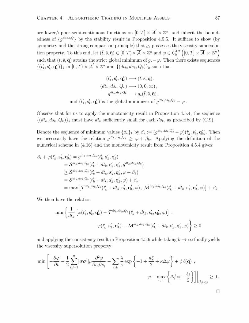
Chapter 4. Algorithmic Trading in Multiple Assets 87
are lower/upper semi-continuous functions on [0, T ] × A′ × Zn, and inherit the bound-
edness of gdt,ds,Q by the stability result in Proposition 4.5.5. It suffices to show (by
symmetry and the strong comparison principle) that g∗ possesses the viscosity supersolu-
tion property. To this end, let (t, s, q) ∈ [0, T )×A′×Zn and ϕ ∈ C1,2b
([0, T ]×A′ × Zn
)such that (t, s, q) attains the strict global minimum of g∗−ϕ. Then there exists sequences
(t′k, s′k,q′k)k in [0, T )×A′ × Zn and (dtk, dsk, Qk)k such that
(t′k, s′k,q
′k) −→ (t, s, q) ,
(dtk, dsk, Qk) −→ (0, 0,∞) ,
gdtk,dsk,Qk −→ g∗(t, s, q) ,
and (t′k, s′k,q
′k) is the global minimizer of gdtk,dsk,Qk − ϕ .
Observe that for us to apply the monotonicity result in Proposition 4.5.4, the sequence
(dtk, dsk, Qk)k must have dtk sufficiently small for each dsk, as prescribed by (C.9).
Denote the sequence of minimum values βkk by βk := (gdtk,dsk,Qk −ϕ)(t′k, s′k,q
′k). Then
we necessarily have the relation gdtk,dsk,Qk ≥ ϕ + βk. Applying the definition of the
numerical scheme in (4.16) and the monotonicity result from Proposition 4.5.4 gives:
βk + ϕ(t′k, s′k,q
′k) = gdtk,dsk,Qk(t′k, s
′k,q
′k)
= Sdtk,dsk,Qk(t′k + dtk, s′k,q
′k, g
dtk,dsk,Qk)
≥ Sdtk,dsk,Qk(t′k + dtk, s′k,q
′k, ϕ+ βk)
= Sdtk,dsk,Qk(t′k + dtk, s′k,q
′k, ϕ) + βk
= max[T dtk,dsk,Qk(t′k + dtk, s
′k,q
′k, ϕ) ,Mdtk,dsk,Qk(t′k + dtk, s
′k,q
′k, ϕ)
]+ βk .
We then have the relation
min
1
dtk
[ϕ(t′k, s
′k,q
′k)− T dtk,dsk,Qk(t′k + dtk, s
′k,q
′k, ϕ)
],
ϕ(t′k, s′k,q
′k)−Mdtk,dsk,Qk(t′k + dtk, s
′k,q
′k, ϕ)
≥ 0
and applying the consistency result in Proposition 4.5.6 while taking k →∞ finally yields
the viscosity supersolution property
min
[−∂ϕ∂t− 1
2
n∑i,j=1
[σσ′]ij∂2ϕ
∂si∂sj−∑i,±
λ
κexp
−1 +
κξ
2+ κ∆ϕ
+ φ `(q) ,
ϕ−maxi ,±
∆±i ϕ−
ξi2
]∣∣∣∣(t,s,q)
≥ 0 .

Chapter 4. Algorithmic Trading in Multiple Assets 88
4.6 Conclusions
This chapter establishes a rigorous framework for a multiple asset economy that exhibits
a specific type of structural dependence, defined as being over-complete. A parsimonious
model is then built upon this framework that adheres to the strict no arbitrage bounds
dictated by the construction of these assets. It is shown that when these assets have non-
zero bid/offer spreads, the economy no longer contains redundant assets; a fundamental
difference between this framework and classical quantitative finance.
An HFT strategy is developed for the investor that both passively submits LOs and
aggressively executes MOs. The corresponding stochastic optimal control problem is
solved when maximizing expected terminal wealth while penalizing open positions via
the investor’s total portfolio risk at each point in time; the multivariate extension to
penalizing via the squared position in one asset at each point in time. Qualitative features
of the optimal trading strategy are investigated and inventory management is, once again,
demontrated to play a key role in the success of the HFT strategy. More specifically,
the investor actively submits her LO quotes in such a way to manage her inventory and
utilize the instantaneous correlation between multiple assets to partially hedge away the
inventory risk associated with a large open position in a less liquid asset.
Through the use of a simulation study and a 2-dimensional illustrative example, we show
the positive effect that trading multiple assets together, rather than trading each one
seperately, has on the investor’s PnL. By using more liquid assets to partially hedge
away risk, the investor can better manage her inventory risk when market making in a
less liquid asset allowing her to be more aggressive, generate more trade flow and hence,
increase her mean PnL for a fixed level of risk. This tradeoff between mean PnL and
risk, whether it be standard deviation of PnL or mean inventory risk, is highlighted by
varying the inventory aversion parameter φ and constructing the corresponding efficient
frontier.
Moreover, the investor can further enhance profits (or reduce risk for a given level of
mean PnL) when her strategy considers where the midprice process, St, is in the no-
arbitrage region. That is, when she considers the structural dependence in addition to
just considering the multiple assets as correlated Brownian Motions. More specifically,
she adjusts her LO quotes and may submit MOs when the midprice process approaches
the boundary of the no-arbitrage region in an attempt to acquire a directional position
in some particular combination of the assets.
An explicit numerical scheme is provided to solve the derived HJBQVI and convergence
results are discussed to ensure that the given discretization scheme converges to the true

Chapter 4. Algorithmic Trading in Multiple Assets 89
viscosity solution. Lastly, we derive a dimensional reduction in the spatial variable for the
midprice which significantly reduces the computational time of the numerical solution,
thus making it viable for practical application.

Chapter 5
The Generalized Latent Hawkes
Process
When analyzing event data, many natural systems exhibit large amounts of clustering.
Although there are cases when such behaviour can be explained by poisson clustering49,
there are several others where self-excitation effects are more pronounced and quiet pe-
riods persist far longer. The modeling of self-exciting event data has been attempted in
a variety of disciplines. Notable applications include seismology (see Ogata (1988) and
Vere-Jones (1995) for the modeling of earthquake data), neuroscience (see Chornoboy
et al. (1988) for the modeling of neural activity), genetics and molecular biology (see
Gusto and Schbath (2005) for the analysis of motif occurrences in DNA sequences via
Hawkes processes), and the social sciences (see Mohler et al. (2011) for the modeling of
criminal activity).
As stated earlier, the classical multivariate Hawkes process (Hawkes (1971)) has recently
been used in the financial econometrics literature to model clustering in trade arrival and
changes in the limit order book (LOB), see Large (2007), Bowsher (2007), Shek (2011),
and Toke (2011). Embrechts et al. (2011) improve upon the classical Hawkes model by
introducing dependency in the marks (in the context marked point processes) via copulas.
However, the fact is that most applications of such a process for modeling purposes do
not have marks that are useful for estimating the jump size in intensity as a part of the
observable data. This is the first work to provide statistical estimation methodologies
for a Hawkes model with a random, unobservable, jump size in the intensity process
(or, more precisely, a marked Hawkes process with unobservable marks). The fact that
49Poisson clustering refers to the fact that clusters of events are likely to occur simply by chance, evenwhen the underlying event arrival rate is constant.
90

Chapter 5. The Generalized Latent Hawkes Process 91
these random jump sizes are latent makes classical likelihood methods computationally
prohibitive.
This chapter is outlined as follows: Section 5.1 motivates this work in the context of
financial microstructure. Section 5.2 presents the model, the form of the data, and some
other probabilistic quantities of interest. Section 5.3 details the first calibration algorithm
which focuses on renewal points (defined in Section 5.2.4) and the isolated likelihood
function (defined in Section 5.3.1). Both asymptotic and sharp analytic bounds on this
pseudo-likelihood function are also provided, as well as a simulation study. Section 5.4
outlines the second calibration algorithm which involves a Sequential Monte Carlo (SMC)
particle filter. Section 5.5 is concerned with the construction of adapted estimators for
the latent intensity process, λt. Finally, Section 5.6 surveys other real-world applications
of the Generalized Hawkes Model within the context of quantitative finance.
Many of the methods derived in this chapter will be put to use on real data in Sections 6.1
and 6.2, and are critical components in the real-world application of the high frequency
trading (HFT) strategy derived in Chapter 3, as will also be applied to real data in Secton
6.3.
5.1 Motivation
As previously eluded to, self-exciting point processes arise in many financial and biological
applications. A point process Mtt≥0 is typically referred to as self-exciting if C[Mt+s−Mt,Mt+s+u−Mt+s] > 0 for all t ≥ 0 and s, u > 0. A particular example of such a process
is the (classical) Hawkes Process where the arrival of each point induces a (constant)
jump in the process’s intensity rate. In many real world applications, the conjecture is
that some points should induce such a (potentially random) jump, while others do not.
In this chapter, we propose such a model and give an efficient calibration algorithm when
the jump indicators are latent.
The main motivation for this work is for application in high frequency trading algorithms.
In particular, the optimal trading strategy derived and discussed in Chapter 3 assumes
that the arrival process of market orders (trades) follows this generalized Hawkes process
with the jump indicator being interpreted as the trade being an influential one. Stated
another way, the jump size random variable is a multiple of a binary random variable.
Observe the fitted intensity in Figure 5.1 (same as Figure 3.1, repeated here for conve-
nience) to Level I financial data50. Notice how the generalized model drastically improves
50Level I data contains event data that corresponds to executed trades with their timestamps and

Chapter 5. The Generalized Latent Hawkes Process 92
0 20 40 60 80 100 1200
5
10
15
20
25
30
Time (seconds)
Inte
nsity
rat
e
Fitted: Full ModelFitted: ρ=1Historical
(a) Arrival of IBM market buy orders
0 20 40 60 80 100 1200
5
10
15
20
25
30
Time (seconds)
Inte
nsity
rat
e
Fitted: Full ModelFitted: ρ=1Historical
(b) Arrival of IBM market sell orders
Figure 5.1: IBM market orders. Historical running intensity versus smoothed fitted in-tensity using a 1 second sliding window for IBM for a 2 minute period, between 3:30pmand 3:32pm, February 1, 2008.
the fitted intensity and hence, the need to extend the model beyond the classical Hawkes
model. One key feature is that the generalized model is better at capturing the sharp
spikes in activity that is present in the data. The extremely low values of the historical
intensities are due to the absence of points in the moving window (something that does
not exist in any model with a baseline rate). The key feature that the full model is
attempting to capture is the extreme clustering of events. As you can see in Figure 5.1,
the full model more closely resembles the data generating process in large clusters; this
will be supported with statistical evidence in Section 6.1.
The estimated parameters for the 30 minute window that contains the data in Figure
5.1 can be found in Table 5.1. The larger estimated jump sizes in the full model are
compensated by the probability that not all points induce a jump in the intensity. This
is what creates the sharper peaks when many points are clustered together while still
preserving the overall mean activity rate. By construction of the calibration algorithm in
Section 5.3.2, both methods produce the same fitted value of the long run mean activity
rate limu→∞
E[λu|Ft], where the filtration Ft is defined in Section 5.2.2.
volumes.

Chapter 5. The Generalized Latent Hawkes Process 93
Classical Model Full Model
ρ 1 0.6520
β1 = β2 180.05 195.15η11 = η22 64.1589 111.4633η12 = η21 55.7357 103.8997
θ1 = θ2 2.1616 1.8148
A−1ζ 6.4695 6.4695
Table 5.1: Parameter estimates used for constructing the plots in Figure 5.1.
5.2 The Generalized Hawkes Process
5.2.1 The Model
Let Nt0≤t≤T be a n-dimensional vector of counting processes with intensity process
λt0≤t≤T satisfying
dλt = β(θ − λt)dt+ η∑Ni,t−dNt (5.1)
and initial condition λ0 ≥ 0. For any fixed t, assume η∑Ni,t− is an n × n random
matrix selected from a finite distribution (independent of t), with each possible matrix
having non-negative entries. From this point forward, we will use the short hand ηt when
referring to η∑Ni,t− and η when referring to a random matrix with the same distribution
(since the distribution is independent of t).
Let p denote the size of the codomain of η and denote each element of η as ηij ≥ 0.
Also, denote the probability weights as ρ =
(1−
p−1∑i=1
ρi, ρ1, . . . , ρp−1
)′. We also have the
constraints θ ∈ Rn has positive entries, β is an invertible n × n matrix with positive
entries, ρ ∈ (0, 1]p with ρ · 1n = 1, and β − E[η] has strictly positive eigenvalues. When
p = 2, we will use ρ when referring to ρ1 as there is only one degree of freedom in the ρ
vector.
The terms in the SDE (5.1) can be interpreted as follows: θ is the baseline intensity
that λt mean-reverts to, and the speed of this mean reversion is dictated by the decay
matrix β. Hence, the term β(θ − λt)dt is responsible for exponential decay to level θ.
The factor ηt is the random jump matrix associated with the event at time t that causes
jump in the intensity process λt and may induce subsequent event arrivals (thus creating
a self-excitation effect).
For each entry ηij of the random matrix, we denote its possible values as ηij(k) for
k = 0, 1, . . . , p − 1 (and the full matrix denoted similarly as η(k)) which has associated

Chapter 5. The Generalized Latent Hawkes Process 94
probability ρk or, in the case of k = 0, has probability 1−p−1∑i=1
ρi. It typically makes sense
to force ηij(k) to be monotonic non-decreasing in k, but we do not require this as there
may be some practical applications where having the reversed order for some i, j makes
sense. Finally, observe that since the process Nt ∈ Zn, we only require a countable
number of each of the ηij,· random variables and therefore have no technical issues in
constructing such a well defined probability space.
Observe that if ρ = 1 (and ηij(0) = 0 for all i, j), then the model reduces to a poisson
process. In particular, if λ0 = θ, then the corresponding poisson process is homogeneous.
If ρ = 1 with non-zero η(0), then the model reduces to the Classical Hawkes process where
every event induces a constant jump in λt. Note the self-excitation effect of a jump of
size ηii, as well as the cross-excitation effect of a jump of size ηij (i 6= j) in the other
intensity processes. This simpler model is referred to as the Classical Hawkes Model (or
the ρ = 1 model).
In real world applications, the random matrix η is typically unobservable. However, since
it has a direct effect on the distribution of the point process Nt, we can use statistical
inference to aid in parameter estimation and the likelihood of potential paths of λt.
5.2.2 The Data
We will assume that data (which we aim to calibrate the generalized Hawkes model to)
is provided in the following form: Let T1, . . . , TN denote the inter-arrival times of the
data points. More precisely, each Ti is an element of [0, T ] × 1, . . . , n, with the first
component being the inter-arrival time of the ith event and the second representing to
which element of the process Nt the arrival point corresponds. Let ti ∈ [0, T ] be the
corresponding ith event time, with the second component being the same as that of Ti.
Define the (completed, right-continuous) filtrations:
F t = σ (Nu0≤u≤t) , (5.2)
Ft = F t ∨ σ (ηu0≤u≤t) . (5.3)
F t is the natural filtration generated by Nt (i.e. it only contains information about the
arrival of points in Nt), while Ft also contains information about the jump sizes ηt in
the intensity process λt. Conditional on F t, it is not possible to determine the intensity
process on the interval [0, t]; however, expanding the filtration to Ft allows one to extract
the exact intensity path.

Chapter 5. The Generalized Latent Hawkes Process 95
Note that the random jump size ηti is not included in the observable data (that is, we
observe the filtration F t, not Ft). This detail is what sets this work apart from previously
published estimation techniques. Although we do not observe ηti , we can still make
inference about it by observing the effect it has on future event arrivals of the process
Nt for t > ti.
5.2.3 Probabilistic Quantities of Interest
Observation 5.2.1. The solution to (5.1) is given by
λt = θ + e−βt(λ0 − θ) +
t∫0
e−β(t−u)ηudNu (5.4)
where ηt is shorthand for η∑Ni,t−.
Applying Ito’s Lemma for jump processes to (5.4) gives Equation (5.1) directly. Also
notice that since Nt is a simple function on compact sets (P - a.s.), the above integral
collapses to a finite sum containing Nt · 1n terms (where 1n denotes the n-dimensional
vector of 1’s), of which only those that have positive jump size are non-zero.
Observation 5.2.2. The long run mean (LRM) activity rate can be computed and is
independent of the current level of intensities:
limu→∞
E[λu|Ft] =(In − β−1E[η]
)−1θ . (5.5)
There are also probabilistic quantities that are not only interesting in their own right,
but also will be of use in particle filtering methods to be discussed in Section 5.5.2.
Observation 5.2.3. The function g(t, l | y) := P[Tk(1) ∈ dt, Tk(2) = l |λtk−1= y] admits
the representation
g(t, l | y) = exp−(θt+ β−1(In − e−βt)(y − θ)
)· 1n·[e−βt(y − θ) · el + θl
]dt (5.6)
for t ≥ 0 and l ∈ 1, . . . , n, where ei is the n-dimensional unit vector with 1 in the ith
component. The survival analogue gsurv.(t | y) := P[Tk(1) > t |λtk−1= y] is given by
gsurv.(t | y) = exp−(θt+ β−1(In − e−βt)(y − θ)
)· 1n. (5.7)
The function g(t, l | y) in Equation (5.6) represents the probability density of observing

Chapter 5. The Generalized Latent Hawkes Process 96
the event Tk = (t, l), given the value of λt at the (k− 1)th event. The function gsurv.(t | y)
in Equation (5.7) is the survivor analogue of this quantity representing the probability
that the kth interarrival time is greater than t.
Observation 5.2.4. The function l(q | y, S1, S2) := P[ηtk = ηS1(1)(q) |λtk−1= y, Tk =
S1, Tk+1 = S2], for q ∈ 0, 1, . . . , p− 1 and y ∈ Rn, admits the representation
l(q | y, S1, S2) =ρq · g (S2 | zq(y))
p−1∑r=0
ρr · g (S2 | zr(y))
(5.8)
with zr(y) = θ + e−βs1(1)(y − θ) + ηS1(1)(r)eS1(2). The survival analogue l(q | y, S1, S2) :=
P[ηtk = ηS1(1)(q) |λtk−1= y, Tk = S1, Tk+1(1) > S2(1)] is obtained by simply replacing
g(·) with gsurv.(·) in Equation (5.8).
The function l(q | y, S1, S2) in Equation (5.8) represents the posterior probability that the
jump induced by the kth event is of type q, given the intensity at tk−1, and the interarrival
times Tk and Tk+1.
5.2.4 Renewal Points
Definition 5.2.5. A data point tk is said to be an ε-renewal point ifn∑i=1
λi,tk−−θiθi
< ε,
where ε > 0 is a free parameter.
Observe that if tk is an ε-renewal point, then λt, for t ≥ tk, is approximately (for all
numerical intents and purposes) independent of Ftk−1(and hence, F tk−1
as well by con-
tainment). This approximation is used in Section 5.3 to efficiently compute likelihoods.
We will also drop the dependence on ε when referring to renewal points as we will fix
ε > 0 at the beginning of the calibration.
Definition 5.2.6. A cluster of events, denoted Cmk , is the set of consecutive points
tk, tk+1, . . . , tk+m with the property that tk is a renewal point. Although (with prob-
ability one) there is no point at t = 0, we define t0 = 0 (so that the set Cm0 makes
sense).

Chapter 5. The Generalized Latent Hawkes Process 97
ηt1
?
ηt2
?
λ0 -
?
λt1 -
?
λt2 -
?
T1
T2
T3
. . .
Figure 5.2: A graphical model representation of dependencies in our self-exciting processwith random jump sizes ηtk .
5.3 Calibration Algorithm I: Isolated Likelihood
Finding traditional maximum likelihood estimators (MLEs) is not numerically feasible
due to the large number of possible sequences ηtkk∈N. For a graphical model representa-
tion of dependencies, see Figure 5.2. The exact likelihood function has computation time
O(pN). For numerical computations, the run time can be reduced to 1m(N)
pm(N) (up to
a multiplicative constant), where m(N) is the size of the largest cluster of points, where
ε is taken to reflect floating point precision, with only the first point being a renewal
point. Although this is still too slow for applications in high freqeuency finance, where
N can easily be 104 and m(104) can still be far too large for practical implementations,
this discussion serves as a motivation for the algorithm developed in Section 5.3.2.
The goal of this calibration algorithm is as follows: We want to find the maximizer x
of a function f(x). Unfortunately, f has exponential computational time (in the total
number of data points, N). We wish to find a function g(x) that has P -time computation
and the same maximizer as f . Such a problem, in general, is extremly difficult to solve.
However, we exploit the structure of the function f to construct g quickly and efficiently
without the need to compute f even once. In particular, we exploit the probabilistic
structure of the model that generates the likelihood function f .
In what follows, we propose an efficient method for calibration to medium to large
datasets via maximizing a pseudo-likelihood function and provide an analytic bound
on how close this function is to the true likelihood function.
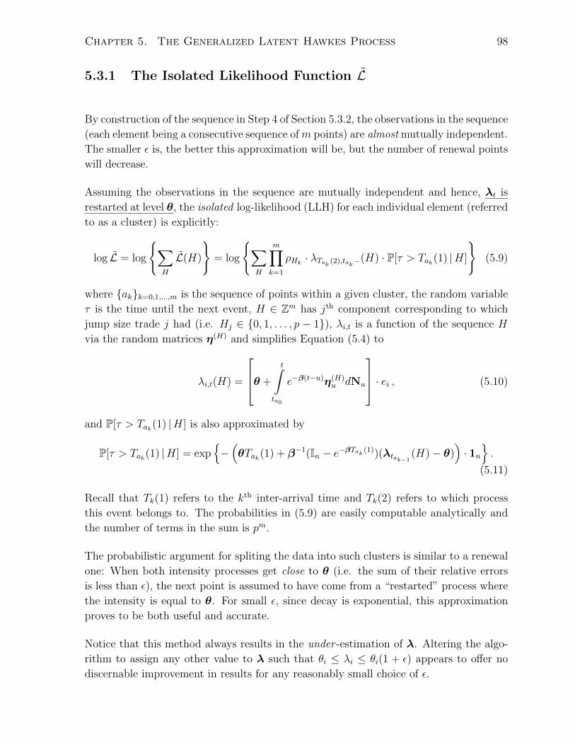
Chapter 5. The Generalized Latent Hawkes Process 98
5.3.1 The Isolated Likelihood Function L
By construction of the sequence in Step 4 of Section 5.3.2, the observations in the sequence
(each element being a consecutive sequence ofm points) are almost mutually independent.
The smaller ε is, the better this approximation will be, but the number of renewal points
will decrease.
Assuming the observations in the sequence are mutually independent and hence, λt is
restarted at level θ, the isolated log-likelihood (LLH) for each individual element (referred
to as a cluster) is explicitly:
log L = log
∑H
L(H)
= log
∑H
m∏k=1
ρHk · λTak (2),tak−(H) · P[τ > Tak(1) |H]
(5.9)
where akk=0,1,...,m is the sequence of points within a given cluster, the random variable
τ is the time until the next event, H ∈ Zm has jth component corresponding to which
jump size trade j had (i.e. Hj ∈ 0, 1, . . . , p − 1), λi,t is a function of the sequence H
via the random matrices η(H) and simplifies Equation (5.4) to
λi,t(H) =
θ +
t∫ta0
e−β(t−u)η(H)u dNu
· ei , (5.10)
and P[τ > Tak(1) |H] is also approximated by
P[τ > Tak(1) |H] = exp−(θTak(1) + β−1(In − e−βTak (1))(λtak−1
(H)− θ))· 1n.
(5.11)
Recall that Tk(1) refers to the kth inter-arrival time and Tk(2) refers to which process
this event belongs to. The probabilities in (5.9) are easily computable analytically and
the number of terms in the sum is pm.
The probabilistic argument for spliting the data into such clusters is similar to a renewal
one: When both intensity processes get close to θ (i.e. the sum of their relative errors
is less than ε), the next point is assumed to have come from a “restarted” process where
the intensity is equal to θ. For small ε, since decay is exponential, this approximation
proves to be both useful and accurate.
Notice that this method always results in the under -estimation of λ. Altering the algo-
rithm to assign any other value to λ such that θi ≤ λi ≤ θi(1 + ε) appears to offer no
discernable improvement in results for any reasonably small choice of ε.

Chapter 5. The Generalized Latent Hawkes Process 99
5.3.2 The Calibration Algorithm
The calibration of the Generalized Hawkes process to data can be perfomed efficiently via
the following fixed-point seeking algorithm. To ensure we have a unique MLE, we impose
the condition that ηij(k), for fixed i, j, is a strictly monotonic function in k. To increase
numerical stability in some datasets, as well as maintain identifiability51, one may want
additional constraints of the form |ηij(k)− ηij(k − 1)| > δij > 0 and ρi > δi > 0.
The calibration methodology can be described as seeking the fixed point of
Q(ξ∣∣T1, · · · , TN
)= ξ with Q
(ξ∣∣Y ) = argsup
ζL(ζ; ξ, Y ), (5.12)
where L is a pseudo-likelihood function that is the product of isolated likelihood functions
of the form of (5.9). The following algorithm provides an efficient way to do this.
1. Fit the data Tjj via maximum likelihood restricting the maximizer to be on
the ρ = 1, 0, 0, . . . , 0 slice of the parameter space. This can be done easily
as the likelihood can be efficiently computed since the intensity path is uniquely
determined given the data Tjj. Appendix E.1 outlines this procedure for the
model described in Section 3.2.2 and is easily generalized.
2. Select free parameters ε = 1100
, and initial guess for ρ which we take to be ρ0 = 1p1p.
With some abuse of notation, compute initial estimate of the codomain of η, namely
η0 which is composed of η0(0),η0(1), . . . ,η0(p−1), by taking η0(j) = 2jp(p−1)
ν where
ν is the ρ = 1 estimate of η from step 1. Take β0 and θ0 as in step 1. Finally, set
k = 0.
3. Compute the upper bound of the intensity path, i.e. the path when ηij,tq =
maxlηij(l) for all q using the current parameter estimates. Observe that this
intensity function dominates all potential intensity functions based on some jumps
being potentially less than the maximum used in the computation (for the fixed
parameter set used).
4. Select the likelihood cluster size m ∈ N and Construct a set of clusters of size m,
Cjkj∈I, where I ⊂ 0, 1, 2, . . . , n is defined by the following recursive criterion:
0 ∈ I, 1, 2, 3, . . . , (m − 1) /∈ I, and j ∈ I (for j > m − 1) whenever tj is a renewal
point and (j −m+ 1), . . . , (j − 1) /∈ I.
5. Due to the condition in step 4, likelihood maximization can now be performed in
a rather efficient way. We want to maximize the isolated likelihood function over
51A family of models is identifiable if for any arbitrary h, EΘ1 [h(·)] = EΘ2 [h(·)] implies Θ1 = Θ2. (i.e.no two distinct models produce the same finite dimensional distributions).

Chapter 5. The Generalized Latent Hawkes Process 100
a specific(n2 − 1 + (n2 + 1)p
)-dimensional subset of the parameter space. If ρ,
β, and (the possible values of) η are free parameters in the isolated likelihood
function (given by Equation (5.9) in Section 5.3.1), then, by using Observation
5.2.2, we constrain the long run mean to remain unchanged by setting
θ =(In − β−1E[η |Θ]
) (In − β−1
k E[η |Θk])−1
θk
where we use Θ to denote an element of the parameter space.
After optimization, set k = k + 1, set ρk, βk, and ηk to the maximizers of the
isolated likelihood function, and
θk =(In − β−1
k E[η |Θk]) (
In − β−1k−1E[η |Θk−1]
)−1θk−1.
6. If ‖ρk−ρk−j‖2 is less than some tolerance (denoted ρ-tolerance) for j = 1, 2, 3, and
if ‖βk−βk−j‖ is less than some other tolerance (denoted β-tolerance) for j = 1, 2, 3,
then break the sequence. We take these tolerances to be 0.001 and 0.1, respectively.
If k reaches an upper bound (we use 9), then break the sequence.
Otherwise, go to step 3.
The constraints in Step 5 are to improve the stability and speed of the algorithm as the
long run mean is fixed in Step 1. As it turns out, and will be confirmed numerically,
the ρ = 1 initial calibration does very well in identifying the correct long run mean of
the model, and we leave the rest of the algorithm to identify where on this subset of the
parameter space the true model resides.
The checks for convergence to a fixed point in Step 6 can be modified to the reader’s
content, as well as the choice of which matrix norm to use. In the simulation study in
Section 5.3.5, we actually consider each component of β seperately for convenience. We
will report the distribution of the break time for simulated data in Section 5.3.5, which
confirms that 9 iterations is sufficient. One thing to keep in mind is that the function
in (5.12) is not continuous in ξ, so a fixed point within the specified tolerances may not
always exist. However, as will be numerically demonstrated later on in this chapter, such
cases result in oscillation between a few values that are quite close together. This case
corresponds to when the true MLE is close to a point that causes as event to switch
between being a renewal point and not being one.

Chapter 5. The Generalized Latent Hawkes Process 101
5.3.3 Bounding the Error of the Isolated Likelihood Function
The renewal point argument given in Section 5.3.1 deserves some technical justification.
We wish to investigate the difference between the approximation of the likelihood of such
a cluster, L, and its true likelihood, L.
Theorem 5.3.1. Asymptotic Bound. The absolute error of the mis-specified (isolated)
likelihood function is
|L − L| = O(ε) (5.13)
for small ε > 0.
Proof. See Appendix C.9.
Theorem 5.3.2. Absolute Error Bound. If β is a diagonal matrix, then we also have
explicit absolute bounds
−m log(1 + ε) < log L − logL < mε‖θ‖n∑j=1
β−1jj . (5.14)
Proof. See Appendix C.10.
For general distribution of η, the bounds in Equation (5.14) are sharp. However, it is
worthy to note that for a pre-specified distribution of η, these bounds can be improved
upon.
5.3.4 Link to Composite Likelihood Methods
Motivated by composite likelihood functions52 associated with Gaussian random fields,
which uses the big blocks method (see Caragea and Smith (2007)), the data is split into
approximately independent blocks.
The Composite Marginal Likelihood (see Chandler and Bate (2007)) formed by the prod-
uct of densities for all the observations in each block and is given by
LMC(Θ; y) =B∏b=1
f(zb; Θ) (5.15)
52For a general survey of composite likelihood functions, see Varin et al. (2011).

Chapter 5. The Generalized Latent Hawkes Process 102
where z1, . . . , zB are B blocks of data and f(z; Θ) is the marginal density of the block z.
In our framework, we choose the blocks of the form tl, . . . , tl+s via the following criteria:
(i) tl and tl+s are renewal points and (ii) tl+1, . . . , tl+s−1 are not renewal points.
In the calibration algorithm described in Section 5.3.2, we have approximated f(zb; Θ) by
f(z′b; Θ), where z′b contains only the firstm interarrival times of zb (or all of zb ifm ≥ s−1).
In the setup of this calibration algorithm, this density can be computed exactly with
reasonable computational time and provides a stable large sample calibration.
5.3.5 Numerical Results on Simulated Data
We find that this calibration algorithm works remarkably well (and efficiently) when
p = 2 and η(0) = 0. It is worthy to note that the generalized Hawkes model proposed
here is already more general than the model posed in Section 3.2.2 since it does not
assume symmetry of the parameters between the two components of Nt, not to mention
that the algorithm is for general dimension n. This section only reports results for n = 2
as that was our motivating example. We restrict β to be diagonal in the calibration
to maintain the bounds in Equation (5.13), and further take β to be a multiple of the
identity matrix for simulation speed (note that this restriction is not imposed on β in
the calibration).
We first present calibration results for the symmetric model posed in Section 3.2.2 of the
single asset market making problem. See Table 5.2 for means and standard deviations
of our estimators using the calibration algorithm outlined in Section 5.3.2. Estimates for
the mean jump size and long run mean are also reported. Notice that as we increase
the sample size N from 500 to 2,000 to 10,000, we get a rapid reduction in the variance
of each estimator. The histograms in Figure 5.3 show the empirical distribution of the
parameter estimates for simulated data for m = 3 on 2,000 data points.
Also notice that as we increase m from 1 to 4, we attain both a reduction in bias and in
the variance of each estimator in larger datasets (N > 2, 000) – although this is at the
expense of runtime. An additional benefit of using a larger cluster size m comes by way
of a more stable fixed-point search, as will be discussed later in this section.
See Table 5.3 for means and standard deviations of our estimators when we do not
assume symmetry (which yields 9 free parameters). Observe that the standard errors of
the estimators has increased slightly over the symmetric case as a result of the increase
in the number of parameters being estimated. The histograms in Figure 5.4 show the
empirical distribution of estimators on simulated data for m = 3 on 2,000 data points.

Chapter 5. The Generalized Latent Hawkes Process 103
N = 500
true m = 1 m = 2 m = 3 m = 4
mean (std) mean (std) mean (std) mean (std)
ρ 0.7 0.753 (0.190) 0.736 (0.177) 0.729 (0.177) 0.729 (0.168)
β 50 52.13 (10.99) 50.86 ( 9.05) 50.30 ( 8.15) 50.63 ( 7.53)η11(1) 25 25.59 ( 9.07) 25.36 ( 7.93) 25.46 ( 7.37) 25.15 ( 6.63)η12(1) 15 15.26 ( 5.91) 15.18 ( 5.18) 15.05 ( 4.61) 15.23 ( 4.22)
θ 1 1.008 (0.153) 1.003 (0.146) 1.016 (0.137) 1.012 (0.141)
E[η11|Θ] 17.5 18.06 ( 4.27) 17.67 ( 3.64) 17.60 ( 3.26) 17.53 ( 3.18)LRM 2.273 2.291 (0.278) 2.287 (0.295) 2.319 (0.289) 2.305 (0.283)
runtime 1.55 ( 0.79) 1.44 ( 0.79) 1.52 ( 0.87) 1.86 ( 1.15)
N = 2,000
ρ 0.7 0.720 (0.113) 0.714 (0.104) 0.709 (0.093) 0.716 (0.097)
β 50 50.28 ( 5.65) 50.28 ( 4.52) 50.28 ( 4.05) 50.27 ( 3.69)η11(1) 25 24.97 ( 4.83) 25.14 ( 4.02) 25.04 ( 3.61) 24.91 ( 3.54)η12(1) 15 14.97 ( 3.07) 14.97 ( 2.49) 15.09 ( 2.36) 14.96 ( 2.26)
θ 1 0.999 (0.078) 1.001 (0.073) 1.006 (0.069) 1.002 (0.068)
E[η11|Θ] 17.5 17.58 ( 2.16) 17.64 ( 1.80) 17.50 ( 1.65) 17.56 ( 1.54)LRM 2.273 2.276 (0.138) 2.281 (0.139) 2.281 (0.136) 2.276 (0.137)
runtime 2.51 ( 0.91) 2.50 ( 1.03) 3.57 ( 1.47) 5.41 ( 2.17)
N = 10,000
ρ 0.7 0.705 (0.049) 0.704 (0.044) 0.703 (0.044) 0.703 (0.043)
β 50 50.21 ( 2.37) 50.10 ( 2.00) 50.12 ( 1.82) 50.00 ( 1.63)η11(1) 25 25.03 ( 2.15) 25.01 ( 1.71) 25.02 ( 1.63) 24.98 ( 1.62)η12(1) 15 15.03 ( 1.34) 14.93 ( 1.09) 15.02 ( 0.98) 14.96 ( 0.98)
θ 1 1.000 (0.034) 1.001 (0.032) 1.002 (0.030) 1.000 (0.031)
E[η11|Θ] 17.5 17.55 ( 0.92) 17.55 ( 0.77) 17.52 ( 0.71) 17.49 ( 0.66)LRM 2.273 2.272 (0.063) 2.272 (0.063) 2.276 (0.063) 2.272 (0.064)
runtime 5.18 ( 1.64) 5.76 ( 1.77) 10.03 ( 3.68) 18.98 ( 7.86)
Table 5.2: Mean and standard deviations of estimators (1,000 simulations) when n =p = 2, η(0) = 0, η11(1) = η22(1), η12(1) = η21(1), β1 = β2, θ1 = θ2, and using AlgorithmI. Total number of free parameters is 5. LRM refers to the long run mean of activityrate of any component of Nt and runtime is in seconds.

Chapter 5. The Generalized Latent Hawkes Process 104
0.4 0.5 0.6 0.7 0.8 0.9 10
20
40
60
80
100
120
ρ
Fre
quen
cy
(a) Frequency of ρ
30 40 50 60 700
20
40
60
80
100
120
β
Fre
quen
cy
(b) Frequency of β
10 15 20 25 30 35 400
20
40
60
80
100
120
η11(1)
Fre
quen
cy
(c) Frequency of η11(1)
0.8 0.9 1 1.1 1.20
20
40
60
80
100
120
θ
Fre
quen
cy
(d) Frequency of θ
10 15 20 250
20
40
60
80
100
120
140
E[η11|Θ]
Fre
quen
cy
(e) Frequency of E(η11|Θ)
1.8 2 2.2 2.4 2.6 2.80
20
40
60
80
100
120
LRM
Fre
quen
cy
(f) Frequency of long run mean
Figure 5.3: Distribution of estimators (1,000 simulations of 2,000 data points) whenn = p = 2, η(0) = 0, η11(1) = η22(1), η12(1) = η21(1), β1 = β2, θ1 = θ2, and usingAlgorithm I with m = 3.

Chapter 5. The Generalized Latent Hawkes Process 105
N = 500
true m = 1 m = 2 m = 3 m = 4
mean (std) mean (std) mean (std) mean (std)
ρ 0.7 0.768 (0.184) 0.748 (0.179) 0.748 (0.179) 0.739 (0.172)
β1 50 52.78 (20.95) 51.88 (14.30) 51.26 (11.98) 51.40 (11.16)
β2 50 53.27 (17.96) 51.21 (13.75) 51.76 (12.33) 50.93 (10.62)η11(1) 25 25.10 (12.02) 25.63 (10.20) 25.05 ( 9.01) 25.30 ( 8.37)η12(1) 15 14.91 ( 7.88) 15.34 ( 6.84) 15.51 ( 6.79) 15.35 ( 5.70)η21(1) 15 15.09 ( 8.22) 15.26 ( 6.47) 15.35 ( 6.14) 15.37 ( 5.76)η22(1) 15 25.60 (12.65) 25.05 ( 9.50) 25.07 ( 8.64) 25.26 ( 8.15)
θ1 1 0.998 (0.175) 0.998 (0.147) 1.008 (0.138) 0.999 (0.133)
θ2 1 1.001 (0.166) 0.992 (0.147) 1.007 (0.134) 0.997 (0.126)
E[η11|Θ] 17.5 18.08 ( 6.98) 18.09 ( 5.60) 17.75 ( 4.88) 17.85 ( 4.61)LRM1 2.273 2.289 (0.277) 2.310 (0.287) 2.324 (0.288) 2.300 (0.289)
runtime 2.26 ( 1.13) 1.98 ( 1.13) 2.10 ( 1.28) 2.50 ( 1.64)
N = 2,000
ρ 0.7 0.720 (0.115) 0.721 (0.105) 0.712 (0.098) 0.717 (0.095)
β1 50 50.30 ( 8.00) 50.52 ( 6.50) 50.53 ( 5.75) 50.52 ( 5.33)
β2 50 50.72 ( 7.80) 50.52 ( 6.48) 50.37 ( 5.72) 50.07 ( 5.18)η11(1) 25 24.96 ( 5.89) 24.86 ( 4.83) 25.21 ( 4.37) 24.92 ( 3.99)η12(1) 15 15.01 ( 3.87) 15.05 ( 3.16) 15.13 ( 2.94) 15.05 ( 2.79)η21(1) 15 15.12 ( 3.87) 14.95 ( 3.22) 15.07 ( 2.81) 14.92 ( 2.73)η22(1) 15 25.17 ( 5.82) 24.83 ( 4.91) 25.01 ( 4.31) 24.77 ( 4.08)
θ1 1 0.999 (0.083) 0.996 (0.071) 0.998 (0.066) 1.000 (0.066)
θ2 1 1.003 (0.081) 1.002 (0.071) 1.001 (0.066) 1.001 (0.066)
E[η11|Θ] 17.5 17.55 ( 3.09) 17.60 ( 2.56) 17.68 ( 2.32) 17.63 ( 2.19)LRM1 2.273 2.281 (0.140) 2.273 (0.135) 2.277 (0.134) 2.281 (0.135)
runtime 3.25 ( 1.29) 3.34 ( 1.48) 4.73 ( 2.09) 7.66 ( 3.34)
N = 10,000
ρ 0.7 0.706 (0.051) 0.704 (0.045) 0.703 (0.044) 0.703 (0.040)
β1 50 50.11 ( 3.28) 50.26 ( 2.75) 49.98 ( 2.59) 50.15 ( 2.29)
β2 50 49.84 ( 3.34) 50.02 ( 2.67) 50.06 ( 2.51) 50.10 ( 2.30)η11(1) 25 24.86 ( 2.53) 25.06 ( 2.08) 24.94 ( 1.88) 25.02 ( 1.82)η12(1) 15 15.02 ( 1.61) 15.05 ( 1.43) 15.00 ( 1.28) 14.99 ( 1.21)η21(1) 15 14.86 ( 1.64) 15.00 ( 1.43) 15.00 ( 1.29) 14.99 ( 1.22)η22(1) 15 24.86 ( 2.60) 24.90 ( 2.07) 25.00 ( 2.02) 24.99 ( 1.76)
θ1 1 1.001 (0.037) 1.000 (0.031) 0.999 (0.031) 1.000 (0.029)
θ2 1 1.000 (0.037) 1.001 (0.033) 1.000 (0.030) 1.000 (0.029)
E[η11|Θ] 17.5 17.46 ( 1.33) 17.58 ( 1.08) 17.47 ( 0.99) 17.54 ( 0.94)LRM1 2.273 2.274 (0.062) 2.273 (0.059) 2.272 (0.060) 2.271 (0.062)
runtime 7.21 ( 2.62) 7.67 ( 2.82) 13.60 ( 5.59) 25.12 (11.20)
Table 5.3: Mean and standard deviations of estimators (1,000 simulations) when n =p = 2 and η(0) = 0 and using Algorithm I. Total number of free parameters is 9.

Chapter 5. The Generalized Latent Hawkes Process 106
0.4 0.5 0.6 0.7 0.8 0.9 10
20
40
60
80
100
ρ
Fre
quen
cy
(a) Frequency of ρ
30 40 50 60 700
20
40
60
80
100
120
β1
Fre
quen
cy
(b) Frequency of β1
10 15 20 25 30 35 400
20
40
60
80
100
120
140
η11(1)
Fre
quen
cy
(c) Frequency of η11(1)
0.8 0.9 1 1.1 1.20
20
40
60
80
100
120
θ1
Fre
quen
cy
(d) Frequency of θ1
10 15 20 250
20
40
60
80
100
120
E[η11|Θ]
Fre
quen
cy
(e) Frequency of E(η11|Θ)
1.8 2 2.2 2.4 2.6 2.80
20
40
60
80
100
120
LRM1
Fre
quen
cy
(f) Frequency of long run mean
Figure 5.4: Distribution of estimators (1,000 simulations of 2,000 data points) whenn = p = 2, η(0) = 0, and using Algorithm I with m = 3. This is the non-symmetriccase.

Chapter 5. The Generalized Latent Hawkes Process 107
It is worthy to point out two things when considering the stated runtimes (which are
stated in seconds). First, the machine that was used to perform these simulations is
considerably old and is considered, by today’s standards, obsolete.53 With this in mind,
it is still useful for comparable relative performance between separate simulations. Sec-
ondly, the code is written in great generality, and can be optimized for specific cases
by hardcoding dimensions and array sizes manually when speed is a priority (i.e. when
deploying such an algorithm in practice). In terms of implementation specifics, MATLAB
is the front end used for all calibrations with specific computations such as computing
likelihood functions or simulating sample paths done in C++ code compiled by MATLAB
into .mexw64 files. If one is truely concerned with speed, making use of a numerical
optimizer in C (or C++) will offer a massive speed advantage over the MATLAB optimizer
that is currently implemented.
To judge the stability of the fixed point search, we look at the tail of the distribution of
the divergence difference of ρ and β, denoted ρdiv and βdiv, respectively. If the algorithm
breaks before the maximum number of iterations is reached, then ρdiv and βdiv are both
set to 0. Otherwise, they are set to the maximum absolute difference between the fitted
value and the value at the last 4 iterations. The 99th percentile and the maximum value
for 2,000 and 10,000 simulations are provided in Tables 5.4 and 5.5, respectively, for
the symmetric case and Tables 5.6 and 5.7 for the non-symmetric case. Notice that
increasing m from 1 to 4 offers a reduction in size of the repeated oscillations of the
diverging sequences ρk and βk constructed in Section 5.3.2. Notice also that increasing
the cluster size m causes the algorithm to exit before the iteration count upper bound on
more sample paths by observing the frequency at iteration count 29 in Figure 5.5. Both
of these features suggest an increase in stability in the fixed point search.
Lastly, consulting Figure 5.5 justifies our choice of an upper bound of 9 iterations, as
enforced in Step 6 of the calibration algorithm.
53Exact specifications include an Intel Pentium E5200 dual-core CPU (2 MB cache, 2.50 GHz) and 8GB DDR3-1,066 MHz RAM.

Chapter 5. The Generalized Latent Hawkes Process 108
m = 1 m = 2 m = 3 m = 4
99th perc. of ρdiv 0.0342 0.0199 0.0163 0.0129maximum of ρdiv 0.0732 0.0399 0.0332 0.0264
99th perc. of β1,div 1.6740 1.2490 0.8702 0.7803maximum of β1,div 3.5301 2.2900 2.1060 1.199099th perc. of β2,div 1.6740 1.2490 0.8702 0.7803maximum of β2,div 3.5301 2.2900 2.1060 1.1990
Table 5.4: Quantities associated with judging fixed point stability. 1,000 simulations of2,000 points when n = p = 2, η(0) = 0, η11(1) = η22(1), η12(1) = η21(1), β1 = β2, θ1 = θ2,and using Algorithm I.
m = 1 m = 2 m = 3 m = 4
99th perc. of ρdiv 0.0049 0.0042 0.0032 0.0026maximum of ρdiv 0.0091 0.0064 0.0057 0.0045
99th perc. of β1,div 0.3137 0.1939 0.1989 0.1574maximum of β1,div 0.8332 0.3935 0.3799 0.278199th perc. of β2,div 0.3137 0.1939 0.1989 0.1574maximum of β2,div 0.8332 0.3935 0.3799 0.2781
Table 5.5: Quantities associated with judging fixed point stability. 1,000 simulations of10,000 points when n = p = 2, η(0) = 0, η11(1) = η22(1), η12(1) = η21(1), β1 = β2,θ1 = θ2, and using Algorithm I.
m = 1 m = 2 m = 3 m = 4
99th perc. of ρdiv 0.0342 0.0244 0.0160 0.0139maximum of ρdiv 0.0575 0.0439 0.0375 0.0282
99th perc. of β1,div 1.9714 1.7593 1.3430 1.4206maximum of β1,div 4.6900 2.9871 2.3766 3.423299th perc. of β2,div 1.8483 1.4009 1.2609 1.1082maximum of β2,div 6.9472 3.4182 2.0013 2.7650
Table 5.6: Quantities associated with judging fixed point stability. 1,000 simulations of2,000 points when n = p = 2, η(0) = 0, and using Algorithm I. This is the non-symmetriccase.

Chapter 5. The Generalized Latent Hawkes Process 109
m = 1 m = 2 m = 3 m = 4
99th perc. of ρdiv 0.0055 0.0041 0.0036 0.0032maximum of ρdiv 0.0099 0.0057 0.0064 0.0058
99th perc. of β1,div 0.3590 0.2643 0.2293 0.2200maximum of β1,div 0.6788 0.4690 0.6056 0.453499th perc. of β2,div 0.3935 0.2902 0.2974 0.2382maximum of β2,div 0.6788 0.5223 0.7381 0.3585
Table 5.7: Quantities associated with judging fixed point stability. 1,000 simulations of10,000 points when n = p = 2, η(0) = 0, and using Algorithm I. This is the non-symmetric case.
0 10 20 30 400
50
100
150
200
250
300
350
Iteration count
Fre
quen
cy
(a) m = 1
0 10 20 30 400
50
100
150
200
250
300
350
Iteration count
Fre
quen
cy
(b) m = 2
0 10 20 30 400
100
200
300
400
500
Iteration count
Fre
quen
cy
(c) m = 3
0 10 20 30 400
100
200
300
400
500
Iteration count
Fre
quen
cy
(d) m = 4
Figure 5.5: Distribution for the number of iterations of the calibration algorithm on 1,000simulations of 2,000 points in the symmetric model.

Chapter 5. The Generalized Latent Hawkes Process 110
5.4 Calibration Algorithm II: Sequential Monte Carlo
Calibration Algorithm I excels when p = 2 and η(0) = 0 with superior speed, but is
not robust and fails to provide meaningful estimators when either η(0) ≥ 0 (interpreted
element-wise) or p > 2. To this end, we introduce a slower, yet more robust method of
calibration that utilizes Sequential Monte Carlo particle filtering (see, e.g., Gordon et al.
(1993), Pitt and Shephard (1999), and Doucet et al. (2000)) . These techniques will also
provide a more reliable method to estimate λt online in Section 5.5.2.
5.4.1 Sequential Monte Carlo & Particle Filtering – Classical
Method
Here we briefly describe the SMC particle filtering algorithm for estimating the distribu-
tion of the hidden states λt1 , . . . ,λtN−1, beginning with M particles at λ0 = θ.
At step k ∈ 2, 3, . . . , N, we have λtk−2and wish to propagate particles i = 1, . . . ,M
forward to get λtk−1.
1. Draw M samples of λtk−1from the posterior distribution
λ(i)tk−1∼ P
[λtk−1
|λtk−2, Tk−1 , Tk
].
(a) compute lk−1(q) := l(q |λtk−2, Tk−1, Tk) (i.e. probability that Hk−1 = q, for
q = 1, . . . , p− 1, given λtn−2 , Tn−1, and Tn) where l(q | y, S1, S2) is provided in
Observation 5.2.4.
(b) Draw iid uniforms u(i) ∼ U(0, 1) for each i = 1, . . . ,M
(c) Use the uniform u(i) to simulate and set H(i)k−1 = q ∈ 0, 1, . . . , p − 1 with
corresponding probability lk−1(q). That is, set
H(i)k−1 = sup
q ∈ 0, 1, . . . , p− 1 :
q−1∑z=0
lk−1(z) ≤ u(i)
(d) Set
λ(i)tk−1
= θ + e−βTk−1(1)(λ(i)tk−2− θ) + η(H
(i)k−1) eTk−1(2)

Chapter 5. The Generalized Latent Hawkes Process 111
2. Compute the un-normalized weights, given the observation Tk
α(i)k =
P[Tk |λtk−1
= λ(i)tk−1
]P[Hk−1 = H
(i)k−1 |λtk−2
= λ(i)tk−2
, Tk−1
]P[Hk−1 = H
(i)k−1 |λtk−2
= λ(i)tk−2
, Tk−1 , Tk
] (5.16)
= g(Tk , H(i)k−1 |λ
(i)tk−1
)×ρH
(i)k−1
lk−1(H(i)k−1)
(5.17)
where g(t, l | y) is provided by Equation (5.6) in Observation 5.2.3.
3. Compute and resample from the normalized weights.
(a) W(i)k = α
(i)k /∑
j α(j)k
(b) Draw a single uniform u ∼ U(0, 1) and define ui = u+i−1M
, i = 1, . . . ,M
(c) Find Ni such that∑Ni−1
j=1 W(j)k ≤ ui ≤
∑Nij=1W
(j)k . The number of “offspring”
for particle i is given by Mi = Ni −Ni−1 (with N0 = 0)
(d) For each λ(i)tk−1
, create Mi offspring and call these λ(i)
tk−1
(e) The updated equally weighted paths of the particles are λ(i)
t1, . . . ,λ
(i)
tk−1
5.4.2 The Calibration Algorithm
Similar to the composite likelihood framework of Section 5.3.4, we split up the density
into the product of conditional densities54 (instead of marginal densities as was done
previously) via
L(Θ; y) = f(z1; Θ)∏k≥2
f(zk; z1, . . . , zk−1,Θ) , (5.18)
where f(zk; ·,Θ) is the conditional density of the kth block of data.
As done in Algorithm I, the simpler ρ = 1 model is calibrated first. While constraining
the long run mean to remain unchanged, we proceed to approximate each factor in
f(z1; Θ)N∏k=2
f(zk; z1, . . . , zk−1,Θ) by particle propagation to estimate the distribution of
λtk−1. More specifically,
1. Propagate the particles to tk−2 as outlined in Section 5.4.1.
2. Decay λt by rate matrix β to tk−1.
54For composite conditional likelihood methods, see Stein et al. (2004).

Chapter 5. The Generalized Latent Hawkes Process 112
3. Add a randomly generated jump η from the prior jump distribution (i.e. the
distribution with probabilities given by ρ).
The explicit details for estimating λt for all t (i.e. not just at event times tk) are given
in Section 5.5.2.
5.4.3 Numerical Results on Simulated Data: η(0) = 0
See Table 5.8 and 5.9 for the means and standard deviations of the estimators using
Algorithm II performed on the two models that were calibrated in Section 5.3.5. Observe
that there is a noticable increase in accuracy at the cost of runtime, especially for N = 500
data points. Notice that the reduction in the estimators’ standard errors over Algorithm
I (across all cluster sizes m = 1, 2, 3, 4) exists even for as few as 10 particles. Figures
5.6 and 5.7 depict the distributions of the aforementioned estimators for N = 2,000 data
points and using 20 particles.

Chapter 5. The Generalized Latent Hawkes Process 113
N = 500
true 10 particles 20 particles 50 particles
mean (std) mean (std) mean (std)
ρ 0.7 0.690 (0.153) 0.690 (0.155) 0.684 (0.157)
β 50 51.93 ( 5.49) 51.76 ( 5.45) 51.38 ( 5.46)η11(1) 25 27.25 ( 6.15) 27.06 ( 6.05) 27.36 ( 6.40)η12(1) 15 16.32 ( 3.99) 16.25 ( 3.85) 16.28 ( 4.03)
θ 1 1.016 (0.131) 1.015 (0.124) 1.019 (0.128)
E[η11|Θ] 17.5 18.07 ( 2.51) 17.91 ( 2.46) 17.90 ( 2.41)LRM 2.273 2.310 (0.287) 2.299 (0.282) 2.312 (0.287)
runtime 4.42 ( 2.72) 8.68 ( 6.88) 21.45 (14.98)
N = 2,000
ρ 0.7 0.717 (0.087) 0.706 (0.089) 0.710 (0.090)
β 50 50.84 ( 2.73) 50.66 ( 2.79) 50.64 ( 2.72)η11(1) 25 24.96 ( 2.86) 25.39 ( 3.08) 25.24 ( 3.12)η12(1) 15 15.04 ( 1.82) 15.19 ( 1.85) 15.18 ( 1.91)
θ 1 1.004 (0.066) 1.006 (0.064) 1.004 (0.061)
E[η11|Θ] 17.5 17.70 ( 1.22) 17.69 ( 1.24) 17.69 ( 1.24)LRM 2.273 2.277 (0.139) 2.279 (0.139) 2.283 (0.140)
runtime 17.64 (31.90) 31.20 (23.78) 89.48 (115.73)
Table 5.8: Mean and standard deviations of estimators (1,000 simulations) when n =p = 2, η(0) = 0, η11(1) = η22(1), η12(1) = η21(1), β1 = β2, θ1 = θ2, and using AlgorithmII. Total number of free parameters is 5.

Chapter 5. The Generalized Latent Hawkes Process 114
N = 500
true 10 particles 20 particles 50 particles
mean (std) mean (std) mean (std)
ρ 0.7 0.667 (0.154) 0.676 (0.159) 0.689 (0.168)
β1 50 52.20 ( 7.71) 52.07 ( 7.40) 52.22 ( 7.79)
β2 50 52.13 ( 7.73) 52.01 ( 7.99) 51.97 ( 7.54)η11(1) 25 28.17 ( 7.46) 27.94 ( 7.53) 27.41 ( 7.72)η12(1) 15 17.11 ( 5.12) 16.90 ( 5.22) 16.80 ( 5.14)η21(1) 15 17.30 ( 5.16) 16.96 ( 4.98) 16.99 ( 5.16)η22(1) 15 28.04 ( 7.36) 27.75 ( 7.44) 27.39 ( 7.60)
θ1 1 1.011 (0.103) 1.011 (0.107) 1.009 (0.110)
θ2 1 1.011 (0.106) 1.012 (0.111) 1.011 (0.104)
E[η11|Θ] 17.5 17.99 ( 3.53) 18.05 ( 3.38) 17.97 ( 3.48)LRM1 2.273 2.293 (0.277) 2.303 (0.283) 2.303 (0.288)
runtime 4.48 ( 3.10) 8.26 ( 5.30) 21.39 (13.68)
N = 2,000
ρ 0.7 0.714 (0.090) 0.707 (0.088) 0.705 (0.089)
β1 50 50.95 ( 3.96) 50.33 ( 3.72) 50.56 ( 4.00)
β2 50 51.06 ( 3.92) 50.67 ( 3.85) 50.58 ( 3.90)η11(1) 25 25.21 ( 3.67) 25.16 ( 3.49) 25.34 ( 3.43)η12(1) 15 15.17 ( 2.31) 15.12 ( 2.18) 15.18 ( 2.19)η21(1) 15 15.28 ( 2.37) 15.21 ( 2.28) 15.14 ( 2.19)η22(1) 15 25.30 ( 3.62) 25.41 ( 3.53) 25.40 ( 3.43)
θ1 1 1.004 (0.054) 0.999 (0.054) 1.002 (0.053)
θ2 1 1.003 (0.053) 1.002 (0.052) 1.002 (0.055)
E[η11|Θ] 17.5 17.75 ( 1.78) 17.57 ( 1.67) 17.65 ( 1.73)LRM1 2.273 2.281 (0.141) 2.275 (0.140) 2.276 (0.140)
runtime 15.79 (14.56) 30.19 (23.03) 75.56 (56.66)
Table 5.9: Mean and standard deviations of estimators (1,000 simulations) when n =p = 2, η(0) = 0, and using Algorithm II. Total number of free parameters is 9.

Chapter 5. The Generalized Latent Hawkes Process 115
0.4 0.5 0.6 0.7 0.8 0.9 10
20
40
60
80
100
120
ρ
Fre
quen
cy
(a) Frequency of ρ
30 40 50 60 700
20
40
60
80
100
120
β
Fre
quen
cy
(b) Frequency of β
10 15 20 25 30 35 400
20
40
60
80
100
120
η11(1)
Fre
quen
cy
(c) Frequency of η11(1)
0.8 0.9 1 1.1 1.20
20
40
60
80
100
120
θ
Fre
quen
cy
(d) Frequency of θ
10 15 20 250
20
40
60
80
100
120
E[η11|Θ]
Fre
quen
cy
(e) Frequency of E(η11|Θ)
1.8 2 2.2 2.4 2.6 2.80
50
100
150
200
LRM
Fre
quen
cy
(f) Frequency of long run mean
Figure 5.6: Distribution of estimators (1,000 simulations of 2,000 data points) whenn = p = 2, η(0) = 0, η11(1) = η22(1), η12(1) = η21(1), β1 = β2, θ1 = θ2, and usingAlgorithm II with 20 particles.

Chapter 5. The Generalized Latent Hawkes Process 116
0.4 0.5 0.6 0.7 0.8 0.9 10
20
40
60
80
100
120
ρ
Fre
quen
cy
(a) Frequency of ρ
30 40 50 60 700
20
40
60
80
100
120
β1
Fre
quen
cy
(b) Frequency of β1
10 15 20 25 30 35 400
20
40
60
80
100
120
140
η11(1)
Fre
quen
cy
(c) Frequency of η11(1)
0.8 0.9 1 1.1 1.20
20
40
60
80
100
120
θ1
Fre
quen
cy
(d) Frequency of θ1
10 15 20 250
20
40
60
80
100
120
E[η11|Θ]
Fre
quen
cy
(e) Frequency of E(η11|Θ)
1.8 2 2.2 2.4 2.6 2.80
20
40
60
80
100
120
LRM1
Fre
quen
cy
(f) Frequency of long run mean
Figure 5.7: Distribution of estimators (1,000 simulations of 2,000 data points) whenn = p = 2, η(0) = 0, and using Algorithm II with 20 particles. This is the non-symmetriccase.

Chapter 5. The Generalized Latent Hawkes Process 117
5.4.4 Numerical Results on Simulated Data: η(0) ≥ 0
As previously mentioned, Algorithm I breaks down when the η(0) = 0 constraint is
relaxed to η(0) ≥ 0 and does not yield meaningful parameter estimates. This simula-
tion study reveals that Algorithm II is robust enough to provide reasonable parameter
estimates in this more generalized setting. Although the runtime is significantly longer
than its η(0) = 0 counterpart (due to the fact that more particles are required to better
approximate the posterior distribution of λt), it is still far faster than currently known
Monte Carle Expectation Maximization (MCEM) algorithms. In terms of running this in
a high frequency trading framework, one can run the calibration in a parallel process and
rely on real-time online updating as discussed in Section 5.5. The observed runtime can
allow re-calibration of parameters as often as every few minutes on a reasonably powered
machine and is a feasable solution in a variety of practical settings.
See Tables 5.10 and 5.11 for means and standard errors of estimators and other quantities
of interest. Figures 5.8 and 5.9 also provide the histograms of the distributions of some
of these statistics. Observe that there is much more variability in the estimators of η(0)
and η(1) (and ρ as well). However, in spite of this, the estimates of the mean jump size
E[η] still have relatively low standard deviation. The algorithm also detects the long run
mean with reasonable accuracy. It is difficult to differentiate two points in the parameter
space that have equal long run mean and mean jump size as the difference between the
likelihood function is extremely small and influenced by noise.
Given this algorithm’s ability to identify long run mean, mean jump size, and extract
reasonable and meaningful parameter estimates while keeping run-time down to a few
minutes, it is clear that it is a useful complimentary method to Algorithm I that performs
well for small samples and/or when η(0) ≥ 0.

Chapter 5. The Generalized Latent Hawkes Process 118
N = 2,000
true 50 particles 200 particles
mean (std) mean (std)
ρ 0.7 0.572 (0.147) 0.592 (0.136)
β 50 49.81 ( 2.70) 49.91 ( 2.76)η11(0) 5 8.07 ( 3.77) 7.06 ( 3.34)η11(1) 25 27.64 ( 5.10) 27.41 ( 4.67)η12(0) 5 7.03 ( 2.54) 6.65 ( 2.43)η12(1) 15 16.20 ( 2.96) 16.19 ( 2.84)
θ 1 1.007 (0.057) 0.997 (0.061)
E[η11|Θ] 19 18.82 ( 1.43) 18.88 ( 1.30)
E[η12|Θ] 12 11.99 ( 0.91) 12.03 ( 1.04)LRM 2.632 2.643 (0.175) 2.630 (0.191)
runtime 72.49 (48.96) 382.85 (317.60)
Table 5.10: Mean and standard deviations of estimators (250 simulations) when n =p = 2, η11(1) = η22(1), η12(1) = η21(1), β1 = β2, θ1 = θ2, and using Algorithm II. Totalnumber of free parameters is 7.

Chapter 5. The Generalized Latent Hawkes Process 119
N = 2,000
true 50 particles 200 particles
mean (std) mean (std)
ρ 0.7 0.589 (0.101) 0.595 (0.102)
β1 50 49.86 ( 3.21) 49.95 ( 3.62)
β2 50 50.24 ( 3.47) 49.83 ( 3.59)η11(0) 5 7.79 ( 3.20) 7.34 ( 3.54)η11(1) 25 27.22 ( 4.26) 27.18 ( 4.44)η12(0) 5 7.11 ( 2.67) 6.16 ( 2.71)η12(1) 15 15.81 ( 3.22) 16.60 ( 3.58)η21(0) 5 6.78 ( 2.91) 5.93 ( 2.74)η21(1) 15 16.06 ( 3.45) 16.47 ( 3.05)η22(0) 5 8.27 ( 3.63) 7.20 ( 3.18)η22(1) 25 27.01 ( 4.34) 27.22 ( 4.23)
θ1 1 1.000 (0.057) 1.005 (0.056)
θ2 1 1.008 (0.061) 1.001 (0.056)
E[η11|Θ] 19 18.96 ( 1.66) 18.87 ( 1.65)
E[η12|Θ] 12 12.03 ( 1.41) 12.12 ( 1.36)
E[η21|Θ] 12 12.10 ( 1.38) 12.05 ( 1.32)
E[η22|Θ] 19 19.03 ( 1.75) 18.86 ( 1.70)LRM1 2.632 2.652 (0.172) 2.654 (0.184)LRM2 2.632 2.656 (0.175) 2.648 (0.175)
runtime 75.79 (61.95) 369.75 (329.47)
Table 5.11: Mean and standard deviations of estimators (250 simulations) when n = p =2 and using Algorithm II. Total number of free parameters is 13.

Chapter 5. The Generalized Latent Hawkes Process 120
0.2 0.4 0.6 0.8 10
10
20
30
40
50
ρ
Fre
quen
cy
(a) Frequency of ρ
30 40 50 60 700
5
10
15
20
25
β1
Fre
quen
cy
(b) Frequency of β1
0 5 10 15 200
5
10
15
20
25
30
η11(0)
Fre
quen
cy
(c) Frequency of η11(0)
10 15 20 25 30 35 400
5
10
15
20
25
30
η11(1)
Fre
quen
cy
(d) Frequency of η11(1)
0 5 10 15 200
5
10
15
20
25
30
η12(0)
Fre
quen
cy
(e) Frequency of η12(0)
10 15 20 25 300
5
10
15
20
25
30
35
η12(1)
Fre
quen
cy
(f) Frequency of η11(2)
Figure 5.8: Distribution of estimators (250 simulations of 2,000 data points) when n =p = 2 and using Algorithm II with 50 particles. This is the non-symmetric case.

Chapter 5. The Generalized Latent Hawkes Process 121
12 14 16 18 20 22 24 260
5
10
15
20
25
E[η11|Θ]
Fre
quen
cy
(a) Frequency of E(η11|Θ)
8 10 12 14 160
5
10
15
20
25
30
E[η12|Θ]F
requ
ency
(b) Frequency of E(η12|Θ)
0.8 0.9 1 1.1 1.20
5
10
15
20
25
30
35
θ1
Fre
quen
cy
(c) Frequency of θ1
2 2.2 2.4 2.6 2.8 3 3.20
5
10
15
20
25
30
35
LRM1
Fre
quen
cy
(d) Frequency of long run mean
Figure 5.9: Distribution of estimators (250 simulations of 2,000 data points) when n =p = 2 and using Algorithm II with 50 particles. This is the non-symmetric case.

Chapter 5. The Generalized Latent Hawkes Process 122
5.5 F t - Adapted Estimators for λt
Sections 5.3 and 5.4 are useful in generating pseudo-likelihood estimators of Θ. However,
even with knowledge of the true value of Θ, it is still no trivial task to recover the latent
process λt. This section provides two methods for real-time estimation of λt.
5.5.1 Via Renewal Points
In this section, we propose a method to estimate the current value of λt after the cali-
bration has been performed. Motivated by the subsequence selection criteria explained
in Step 4 of Section 5.3.2, we compute an estimator for λt as follows: Suppose you want
to compute λt with t ∈ [tk, tk+1).
1. Find k0 ≤ k such that tk0 is a renewal point, but tk0+1, . . . , tk are not renewal points.
2. Assume λtk0− = θ. Compute the pk−k0+1 possible values of λtk (and hence, λt as
well). Denote the possible values of λt as λ(i).
3. Compute the posterior probability of each value of λ(i) in Step 2 using the approx-
imation
P[λt = λ(i) | F t
]≈ P
[λt = λ(i)
∣∣σ (Nuu∈[tk0 ,t]
), λtk0 = θ
]. (5.19)
The details of this computation can be found in Appendix E.4.
4. Take the estimator λt to be the posterior mean. More generally, one could take
λt such that h(λt) is (conditional on the observed data) unbiased for h(λt), where
h : Rn+ → Rn.
Observe that the simplifying approximation in Step 2 becomes more accurate as ε ↓ 0.
However, the smaller ε is, the more inefficient this algorithm becomes since (for a fixed t)
k0 decreases as ε decreases. Hence, the number of total paths can quickly become quite
large if ε is unreasonably small.
5.5.2 Via Sequential Monte Carlo
This method was used in producing this chapter’s motivating plots in Figure 5.1. Fur-
thermore, we propose this to be the method used in constructing on-the-fly estimators

Chapter 5. The Generalized Latent Hawkes Process 123
for λt for use in the optimal HFT strategy in the setting of Chapter 3.
Section 5.4.1 outlines the classical method for particle filtering using Sequential Monte
Carlo. However, we need a way to estimate λtk that is F tk measurable. Unfortunately,
classical SMC methods do not address this issue, nor do they provide a way to estimate
λt when t is not the arrival time of an event. That is, we seek an estimator λt such
that: If G is a σ-algebra on Ω with λt ∈ G, then for any event time tk ≤ t, we must have
G ⊆ F tk if and only if t = tk.
To this end, we first consider the state of the particles at tk−1 via classical SMC methods
(as in Section 5.4.1). We can then use the survival probability (no event yet after the kth
event) to find the posterior probability that the kth event induced a particular jump ηk,
propagate the particles forward to get an estimate of the posterior distribution of λtk ,
and exponentially decay this value forward to find λt. The full details of this modified
SMC particle filter are given as follows:
Let t ∈ [tk, tk+1) for some k ∈ N and denote Tk+1,surv. as the observation that the inter-
arrival time of the (k + 1)th event is right truncated at t− tk.
1. Using the method in Section 5.4.1, propagate the particles to tk−1.
2. Draw M samples of λtk from the posterior distribution
λ(i)tk∼ P
[λtk |λtk−1
, Tk , Tk+1,surv.
].
(a) Compute lk,surv.(q) := lsurv.(q |λtk−1, Tk, Tk+1,surv.) (i.e. probability thatHn−1 =
q, for q = 1, . . . , p− 1, given λtk−1, Tk, and Tk+1,surv.) where lsurv.(q | y, S1, S2)
is provided in Observation 5.2.4.
(b) Draw iid uniforms u(i) ∼ U(0, 1) for each i = 1, . . . ,M
(c) Use the uniform u(i) to simulate and set H(i)k = q ∈ 0, 1, . . . , p − 1 with
corresponding probability lk,surv.(q). That is, set
H(i)k−1 = sup
q ∈ 0, 1, . . . , p− 1 :
q−1∑z=0
lk,surv.(z) ≤ u(i)
(d) Set
λ(i)tk
= θ + e−βTk(1)(λ(i)tk−1− θ) + η(H
(i)k ) eTk(2)

Chapter 5. The Generalized Latent Hawkes Process 124
3. Compute the un-normalized weights, given the observation Tk+1,surv.
α(i) =P[Tk+1,surv. |λtk = λ
(i)tk
]P[Hk = H
(i)k |λtk−1
= λ(i)tk−1
, Tk
]P[Hk = H
(i)k |λtk−1
= λ(i)tk−1
, Tk , Tk+1,surv.
] (5.20)
= gsurv.(Tk+1,surv. |λ(i)tk
)×ρH
(i)k
lk,surv.(H(i)k )
(5.21)
where g(t, l | y) is provided by Equation (5.7) in Observation 5.2.3.
4. Compute and resample from the normalized weights.
(a) W (i) = α(i)/∑
j α(j)
(b) Draw a single uniform u ∼ U(0, 1) and define ui = u+i−1M
, i = 1, . . . ,M
(c) Find Ni such that∑Ni−1
j=1 W (j) ≤ ui ≤∑Ni
j=1W(j). The number of “offspring”
for particle i is given by Mi = Ni −Ni−1 (with N0 = 0)
(d) For each λ(i)tk
, create Mi offspring and call these λ(i)
tk
(e) The updated equally weighted paths of the particles are λ(i)
t1, . . . ,λ
(i)
tk−1
5. Decay the resulting particles at tk exponentially with decay rate matrix β to get
λ(i)
t = θ + e−β(t−tk)(λ
(i)
tk− θ
). (5.22)
Note that we have already resampled under the posterior probabilities given this
survival event. Hence, the particles at time t still have uniform probability.
See Figure 5.10 for a visual depiction of the mean of 3 particles propagating through
time. At any time t, the value of the particle is conditional on F t, not F tk . Observe how
in some instances the particles experience sudden drops during exponential decay. This
is due to the fact that just after the arrival of an event, there is little information about
whether or not the event induced a jump in the particle. However, as time evolves with
the absence of the arrival of the next event, the posterior probability that the previous
event induced a large jump decreases and eventually some particles now do not experience
the aforementioned jump. Hence, there is a downwards jump in the adapted propagation
of such particles. This is easy to visualize due to the small number of particles used in
the SMC particle filter (only 3 in this plot). As the number of particles becomes large,
this effect will be smoothed out and will cause the mean of all the particles to decay
faster than rate β (the decay may no longer be exponential, but the resulting intensity
is less than that if it decayed exponentially with rate β).

Chapter 5. The Generalized Latent Hawkes Process 125
3.5 3.55 3.6 3.65 3.7 3.750
10
20
30
40
t
λ−
t
λ+
t
Figure 5.10: Propagation of the progressively measureable particle filter using the meanof 3 particles via SMC with simulated data.
Furthermore, the mean jump size in the particles at the next event will be at least
E[η]. If the next event occurs shortly after the previous one, then some of the particles
may exhibit an additional jump due to the fact that the previous event may now be
considered to be one that induces a large jump in λt. Such behaviour is a byproduct
of the posterior probability of the previous point causing a large jump in λt being high
when the next event occurs very shortly thereafter. Because the particle propagation
must be F t-adapted, this posterior probability does not increase until the time of the
next event.
To get the point estimator λt, first notice that conditional on F t, the posterior probability
of each particle is equal. With a slight abuse of notation, denote the ith particle as
λ(i)t . Observe that the estimators λt = 1
M
M∑i=1
λ(i)t are approximately unbiased for λt
(given the calibrated parameters are correct), where M is the number of particles. The
approximation is due to the left limit of λ at renewal points being very close to θ, but not
actually equal to θ. Since the conditional distribution of λt is uniform over the particles,
computing unbiased estimators for a given function of λt is a trivial numerical task.
5.6 Other Applications
Within the context of quantitative finance, self-exciting latent processes can be used to
model the default times of corporate bonds in multiple sectors. This has been studied
in Azizpour and Giesecke (2008), where the classical Hawkes process is applied to such
data. The authors also provide filtering methods when the intensity process is masked by
a latent diffusion process. The extension to the case where the jump size for each event

Chapter 5. The Generalized Latent Hawkes Process 126
is both latent and random is a natural one as the default of a large cap corporate bond
would have a very different effect on a macroscopic level than that of a start-up firm.
The use of the multivariate Hakwes model in market microstructure has been studied in
a variety of flavours. Large (2007) explores a stylized framework where he distinguishes
between market orders (MOs) and limit orders (LOs) based on whether or not they cause
a change in the market price. Bacry and Muzy (2013) jointly model the arrival of MOs
and the up/down ticks in a 4-dimensional Hawkes process.
Continuing with this theme, one could attempt to (exogenously) model just the tick
movements in a way that also distinguishes between an uptick due to the bid price
increasing versus the ask price increasing for the purposes of price and liquidity prediction.
These two events are fundamentally different as the former results in a tighter bid/offer
spread, whereas the latter results in a wider spread. This subtle distinction is typically
lost in the modelling choice (although it is recoverable in the framework that Large (2007)
poses).
To this end, one could classify market movements as one of four types: the best bid
price moves up or down, and the best offer price moves up or down. The cause of
such movements can be one of three basic types (MO submission, LO cancellation, LO
submitted inside the spread). It is observed that certain movements in the BBO tend
to cluster together and cross-excite other movements of a particular type. For example,
an increase in the best offer price may be likely to induce the arrival of LOs to the offer
side causing the next event to be a reduction in the best offer price. Or perhaps the data
suggests that an increase in the best offer will self-excite more increases of the same type,
but will also cross-excite increases in the best bid price. This will ultimately create a
short term upward pressure on the price for this asset.
Finally, as eluded to at the beginning of this chapter, there are several cross-disciplinary
applications of the Classical Hawkes Model that the author feels are also worth exploring
in the context of the more generalized process presented in Section 5.2.1.

Chapter 6
Application to Real Data
This chapter applies some of the theoretical results developed throughout previous chap-
ters of this thesis to real tick-by-tick event data for two equities trading on the NASDAQ
exchange and one equity on the NYSE. Sections 6.1 and 6.2 apply the calibration method-
ologies of Sections 5.3 (Algorithm I) and 5.4 (Algorithm II), respectively, where parameter
estimates and some model adequacy diagnostics are reported. Section 6.3 discusses the
performance of the single asset market making strategy derived in Chapter 3 (with a
slight modification for market orders, described in Section 6.3.1). Parameter estimates
from Section 6.1.1, combined with the modified on-the-fly particle filtering method devel-
oped in Section 5.5.2, are the tools used to construct on-the-fly estimates of λt (adapted
to the smaller, observable filtration F t).
6.1 Statistical Results: Generalized Latent Hawkes
Process when η(0) = 0
In this section, we apply Algorithm I with cluster size m = 4, as described in Section
5.3.2, to the symmetric 2-dimensional Hawkes model used in Chapter 3, as well as the
non-symmetric case. For this entire section, we impose the constraint that η(0) = 0.
6.1.1 Parameter Estimates
The raw data is comprised of LOB events which classifies all events as executed market
orders (MOs), limit order (LO) submissions, and LO cancellations. A typical trading day
127

Chapter 6. Application to Real Data 128
BBBY MSFT TEVA
mean (std) mean (std) mean (std)
ρ 0.776 (0.171) 0.412 (0.087) 0.766 (0.171)
β 97.42 (27.13) 105.35 (27.13) 115.64 (33.01)η11(1) 49.16 (16.05) 125.76 (31.53) 61.57 (18.59)η12(1) 6.57 ( 2.37) 19.39 ( 6.62) 11.88 ( 4.16)
θ 0.085 (0.041) 0.157 (0.075) 0.105 (0.054)
E[η11|Θ] 36.80 (10.87) 51.53 (15.75) 45.89 (13.46)
E[η12|Θ] 4.95 ( 1.72) 7.92 ( 2.89) 8.97 ( 3.44)LRM 0.151 (0.076) 0.371 (0.240) 0.206 (0.117)
Table 6.1: Mean and standard deviations of estimators on historical data when n = p = 2,η(0) = 0, η11(1) = η22(1), η12(1) = η21(1), β1 = β2, θ1 = θ2, and using Algorithm I with acluster size of m = 4. Total number of free parameters is 5. LRM refers to the long runmean of activity rate of any component of Nt, given by Lemma 3.2.2. Sample consistsof disjoint 60-minute windows between 10:00am and 4:00pm from Jan-May 2011.
could have anywhere from 200,000 to 1,000,000 total events per equity, of which contain
5,000 to 50,000 market orders (after amalgamation – the exchange records a separate
entry when a MO fills multiple LO quotes; partial fills are also treated as a single MO).
The LOB must be reconstucted from this raw data by keeping track of all existing LO
quotes and updating it with submissions, cancellations, and executions.
We perform a calibration to disjoint 60 minute windows between 10:00am and 4:00pm,
for the months January to May of 2011. Although each window is treated equally in the
sample, this could be refined by considering different periods throughout the trading day
(morning, afternoon, and close). The analysis is performed for the three tickers BBBY (Bed
Bath and Beyond Inc.), MSFT (Microsoft Corporation), and TEVA (Teva Pharmaceutical
Industries Ltd). See Tables 6.1 and 6.2 for results for the symmetric model (as described
in Chapter 3) and its non-symmetric version, respectively. We also provide histograms
of the fitted parameters for the symmetric model in Figure 6.1.
Observe from Table 6.2 that even if we do not impose the symmetry conditions in the
calibration, that the maximum likelihood estimators (MLEs) still produce symmetric
estimates of the parameters (in mean). A simple check to see if there is negative correla-
tion between these parameters (they can still be equal in mean, but be heavily negatively
correlated) is to check their empirical correlation. Table 6.3 shows that the empirical cor-
relations for all the quantities in question are positive. In favour of sparsity, we continue
the analysis in this section only focusing on the symmetric model.

Chapter 6. Application to Real Data 129
BBBY MSFT TEVA
mean (std) mean (std) mean (std)
ρ 0.789 (0.168) 0.419 (0.088) 0.777 (0.168)
β1 99.43 (36.79) 107.07 (33.61) 119.01 (44.02)
β2 100.60 (37.12) 107.74 (32.74) 117.37 (38.16)η11(1) 49.95 (20.49) 124.87 (38.22) 63.32 (23.13)η12(1) 6.91 ( 3.14) 20.85 ( 8.73) 12.47 ( 5.58)η21(1) 6.35 ( 3.26) 19.23 ( 8.69) 11.74 ( 5.53)η22(1) 49.61 (20.95) 129.48 (39.37) 60.63 (22.37)
θ1 0.085 (0.042) 0.163 (0.084) 0.104 (0.056)
θ2 0.084 (0.044) 0.149 (0.082) 0.105 (0.057)
E[η11|Θ] 38.16 (14.57) 51.99 (18.03) 48.05 (17.43)
E[η12|Θ] 5.31 ( 2.40) 8.59 ( 3.60) 9.57 ( 4.65)
E[η21|Θ] 4.85 ( 2.31) 7.95 ( 3.57) 8.93 ( 4.15)
E[η22|Θ] 37.72 (14.43) 53.49 (17.50) 45.70 (15.77)LRM1 0.155 (0.079) 0.389 (0.257) 0.209 (0.123)LRM2 0.150 (0.078) 0.364 (0.244) 0.204 (0.117)
Table 6.2: Mean and standard deviations of estimators on historical data when n = p = 2,η(0) = 0, and using Algorithm I with a cluster size of m = 4. LRM refers to the long runmean of activity rate of Nt, given by Lemma 3.2.2. Sample consists of disjoint 60-minutewindows between 10:00am and 4:00pm from Jan-May 2011.
BBBY MSFT TEVA
corr(β1, β2) 0.074 0.208 0.267corr(η11(1), η22(1)) 0.220 0.206 0.294corr(η12(1), η21(1)) 0.186 0.234 0.176
corr(θ1, θ2) 0.812 0.618 0.828
Table 6.3: Sample correlation of selected pairs of estimators when the calibration doesnot impose symmetry.

Chapter 6. Application to Real Data 130
0 0.2 0.4 0.6 0.8 10
50
100
150
200
ρ
Fre
quen
cy
BBBYMSFTTEVA
(a) Frequency of ρ
0 50 100 150 2000
50
100
150
200
β
Fre
quen
cy
BBBYMSFTTEVA
(b) Frequency of β
0 50 100 150 2000
50
100
150
200
250
300
η11(1)
Fre
quen
cy
BBBYMSFTTEVA
(c) Frequency of η11(1)
0 0.1 0.2 0.3 0.40
50
100
150
200
250
θ
Fre
quen
cy
BBBYMSFTTEVA
(d) Frequency of θ
0 20 40 60 80 1000
50
100
150
200
E[η11|Θ]
Fre
quen
cy
BBBYMSFTTEVA
(e) Frequency of E(η11|Θ)
0 0.2 0.4 0.6 0.8 10
100
200
300
400
LRM
Fre
quen
cy
BBBYMSFTTEVA
(f) Frequency of LRM
Figure 6.1: Frequency of parameter estimates when constrained to n = p = 2, η(0) = 0,η11(1) = η22(1), η12(1) = η21(1), β1 = β2, θ1 = θ2, and using Algorithm I. Sample consistsof disjoint 60-minute windows between 10:00am and 4:00pm from Jan-May 2011.

Chapter 6. Application to Real Data 131
BBBY MSFT TEVA
N 546 1347 1286ρ 0.701 0.331 0.564
β 118.34 66.94 103.37η11(1) 69.17 103.56 82.60η12(1) 10.60 10.24 17.39
θ 0.041 0.084 0.082
Table 6.4: Parameter estimates used for PIT and P-P model diagnotics for the 2:00-3:00window of May 31, 2011.
BBBY MSFT TEVA
N 1526 2898 1738ρ 0.482 0.373 0.605
β 90.93 80.02 100.63η11(1) 69.54 91.83 59.72η12(1) 8.42 14.66 11.63
θ 0.126 0.176 0.137
Table 6.5: Parameter estimates used for PIT and P-P model diagnotics for the 3:00-4:00window of May 31, 2011.
6.1.2 Model Validation: Probability Integral Transform
All model diagnostics performed in this section are done with isolated likelihood cluster
size m equal to 4 for Algorithm I from Section 5.3.2. We use data from the last two
60-minute windows (2:00-3:00 and 3:00-4:00) of the last day in the period used in Section
6.1 (May 31, 2011). The parameter estimates for these 60-minute windows can be found
in Tables 6.4 and 6.5, respectively.
The Probability Integral Transform (PIT; see Thorarinsdottir (2013)) is a transformation
of each interarrival time into a random variable supported on the unit interval. Under
the true model, this is an iid sequence of uniform random variables on [0, 1]. Exact PIT
quantites can be computed using the following decomposition:
P[Tk(1) > Tk,obs(1) |F tk−1
]=∑
i
P[Tk(1) > Tk,obs(1) |λtk−1
= λ(i)]P[λtk−1
= λ(i) |F tk−1
].
(6.1)

Chapter 6. Application to Real Data 132
&%'$λ
(i)
tk−2-
expdecay&%'$λ
(i)
tk−1−-
jumpfromprior&%'$λ
(i)
tk−1=⇒ distribution of Tk
Figure 6.2: A workflow diagram representing the PIT calculation of the ith particle forthe kth interarrival time Tk.
Further notice that the last probability is a posterior probability of a particular value of
λ given the data. The details regarding the computation of this quantity can be found
in Appendix E.4. Since we are conditioning on F tk−1(the filtration at the time of an
event), we do not need to include a survival probability since the last event.
Note that time to compute the posterior distribution of λt at the end of a cluster of
size n is O(2n). Due to this computational complexity, we use Sequential Monte Carlo
(SMC) with 100 particles to efficiently approximate the PIT quantities. To calculate
the survival probability associated with the kth interarrival time, we first propagate the
particles to tk−2, then decay them exponentially to tk−1 and add a jump with probability
ρ. A workflow diagram of this method is given in Figure 6.2. As discussed in Section
5.5.2, the state of the particle at tk−1 must be F tk−1measurable and, as described there,
this induces some subtlety in its simulation.
Figures 6.3 and 6.4 show the distribution of the PIT quantities (for comparison purposes,
the Poisson case is also shown). If the model is correct, then the PIT should produce
iid uniform-(0, 1) random variables. A higher order test for uncorrelated uniforms is to
look at the sample auto-correlation function. Figures 6.5 and 6.6 show the corresponding
auto-correlation functions.
Observe the drastic improvement over the poisson case (the constant mean of the poisson
case is taken to be equal to the long run mean in the full model). The autocorrelation at
several lags is also statistically significantly positive when the poisson model is assumed,
which is consistent with the notion of self-excitation of event arrivals. Although there are
some lags for the Generalized Hawkes model that are statistically significantly different
from zero, the deviation from zero autocorrelation and level of significance is far more
prominent in the case of the Poisson process. Some deviation is expected since we
acknowledge that the parsimonious model we are fitting is not 100% perfect.

Chapter 6. Application to Real Data 133
0 0.2 0.4 0.6 0.8 10
10
20
30
40
50
60
PIT quantity
Fre
quen
cy
(a) Generalized Hawkes: BBBY
0 0.2 0.4 0.6 0.8 10
50
100
150
200
250
300
PIT quantity
Fre
quen
cy
(b) Poisson: BBBY
0 0.2 0.4 0.6 0.8 10
20
40
60
80
100
PIT quantity
Fre
quen
cy
(c) Generalized Hawkes: MSFT
0 0.2 0.4 0.6 0.8 10
100
200
300
400
500
PIT quantity
Fre
quen
cy
(d) Poisson: MSFT
0 0.2 0.4 0.6 0.8 10
20
40
60
80
100
PIT quantity
Fre
quen
cy
(e) Generalized Hawkes: TEVA
0 0.2 0.4 0.6 0.8 10
100
200
300
400
500
PIT quantity
Fre
quen
cy
(f) Poisson: TEVA
Figure 6.3: Distribution of the PIT quantities when constrained to n = p = 2, η(0) = 0,η11(1) = η22(1), η12(1) = η21(1), β1 = β2, θ1 = θ2, and using Algorithm I for the 2:00-3:00window.

Chapter 6. Application to Real Data 134
0 0.2 0.4 0.6 0.8 10
50
100
150
200
PIT quantity
Fre
quen
cy
(a) Generalized Hawkes: BBBY
0 0.2 0.4 0.6 0.8 10
100
200
300
400
500
600
PIT quantity
Fre
quen
cy
(b) Poisson: BBBY
0 0.2 0.4 0.6 0.8 10
50
100
150
200
250
PIT quantity
Fre
quen
cy
(c) Generalized Hawkes: MSFT
0 0.2 0.4 0.6 0.8 10
200
400
600
800
1000
1200
PIT quantity
Fre
quen
cy
(d) Poisson: MSFT
0 0.2 0.4 0.6 0.8 10
20
40
60
80
100
120
140
PIT quantity
Fre
quen
cy
(e) Generalized Hawkes: TEVA
0 0.2 0.4 0.6 0.8 10
100
200
300
400
500
600
700
PIT quantity
Fre
quen
cy
(f) Poisson: TEVA
Figure 6.4: Distribution of the PIT quantities when constrained to n = p = 2, η(0) = 0,η11(1) = η22(1), η12(1) = η21(1), β1 = β2, θ1 = θ2, and using Algorithm I for the 3:00-4:00window.

Chapter 6. Application to Real Data 135
0 2 4 6 8 10−0.2
0
0.2
0.4
0.6
0.8
1
Lag
Sam
ple
Aut
ocor
rela
tion
Sample Autocorrelation Function
(a) Generalized Hawkes: BBBY
0 2 4 6 8 10−0.2
0
0.2
0.4
0.6
0.8
1
Lag
Sam
ple
Aut
ocor
rela
tion
Sample Autocorrelation Function
(b) Poisson: BBBY
0 2 4 6 8 10−0.2
0
0.2
0.4
0.6
0.8
1
Lag
Sam
ple
Aut
ocor
rela
tion
Sample Autocorrelation Function
(c) Generalized Hawkes: MSFT
0 2 4 6 8 10−0.2
0
0.2
0.4
0.6
0.8
1
Lag
Sam
ple
Aut
ocor
rela
tion
Sample Autocorrelation Function
(d) Poisson: MSFT
0 2 4 6 8 10−0.2
0
0.2
0.4
0.6
0.8
1
Lag
Sam
ple
Aut
ocor
rela
tion
Sample Autocorrelation Function
(e) Generalized Hawkes: TEVA
0 2 4 6 8 10−0.2
0
0.2
0.4
0.6
0.8
1
Lag
Sam
ple
Aut
ocor
rela
tion
Sample Autocorrelation Function
(f) Poisson: TEVA
Figure 6.5: Autocorrelation function of the PIT quantities when constrained to n = p = 2,η(0) = 0, η11(1) = η22(1), η12(1) = η21(1), β1 = β2, θ1 = θ2, and using Algorithm I forthe 2:00-3:00 window. The blue lines indicate 95% confidence intervals.

Chapter 6. Application to Real Data 136
0 2 4 6 8 10−0.2
0
0.2
0.4
0.6
0.8
1
Lag
Sam
ple
Aut
ocor
rela
tion
Sample Autocorrelation Function
(a) Generalized Hawkes: BBBY
0 2 4 6 8 10−0.2
0
0.2
0.4
0.6
0.8
1
Lag
Sam
ple
Aut
ocor
rela
tion
Sample Autocorrelation Function
(b) Poisson: BBBY
0 2 4 6 8 10−0.2
0
0.2
0.4
0.6
0.8
1
Lag
Sam
ple
Aut
ocor
rela
tion
Sample Autocorrelation Function
(c) Generalized Hawkes: MSFT
0 2 4 6 8 10−0.2
0
0.2
0.4
0.6
0.8
1
Lag
Sam
ple
Aut
ocor
rela
tion
Sample Autocorrelation Function
(d) Poisson: MSFT
0 2 4 6 8 10−0.2
0
0.2
0.4
0.6
0.8
1
Lag
Sam
ple
Aut
ocor
rela
tion
Sample Autocorrelation Function
(e) Generalized Hawkes: TEVA
0 2 4 6 8 10−0.2
0
0.2
0.4
0.6
0.8
1
Lag
Sam
ple
Aut
ocor
rela
tion
Sample Autocorrelation Function
(f) Poisson: TEVA
Figure 6.6: Autocorrelation function of the PIT quantities when constrained to n = p = 2,η(0) = 0, η11(1) = η22(1), η12(1) = η21(1), β1 = β2, θ1 = θ2, and using Algorithm I forthe 3:00-4:00 window. The blue lines indicate 95% confidence intervals.

Chapter 6. Application to Real Data 137
6.1.3 Model Validation: Probability-Probability Plots
By the theory of point processes, it is well known that for any point process Ptt≥0 with
unique points and limt→∞
Pt = ∞, there exists a random time change t 7−→ τ(t) such that
Pτ(t)t∈R+ is a Poisson Process with unit intensity (see Daley and Vere-Jones (2007)). In
this section, we will perform a random time-change and construct probability-probability
(P-P) plots55 for the time-changed process as a diagnostic for model appropriateness.
In the classical ρ = 1 case, the intensity process λt is observable. In this case, to convert
N−t + N+t t into a Poisson Process, we know exactly what this random time change
should be and is given by
Ti 7−→Ti∫
0
(λ−s + λ+s )ds. (6.2)
However, for the full model, λt is not F t measurable. So we must estimate it given the
data. We propose the following random time change for the purpose of generating a P-P
plot:
Ti 7−→Ti∫
0
(λ−s + λ+
s
)ds (6.3)
where λt is taken to be the mean of the F ti−1measurable particles at time t (propagated
forward with exponential decay). The reason that we do not want to take λt as the mean
of the F t-measurable particles is because we do not want λt, for t ∈ (ti−1, ti), to contain
any information about Ti.
Figure 6.7 is a comparison of P-P plots between the classical Hawkes model (ρ = 1),
the full model, and the Poisson model. The jump sizes in the classical Hawkes case are
scaled down to reflect the increase in ρ to ρ = 1 (the mean jump size and long run mean
activity rates are both preserved).
Notice how the time changed quantiles of the full model better track the exponential
quantiles. Divergence of dense clusters of points in the P-P plot from the 45-line can
be interpreted as model inadequacy, and even more so when the P-P plot possesses
discernable curvature. Such patterns are experienced throughout the collected data.
These plots continue to expose the drastic inadequacy of the Poisson model over the
classical Hawkes model, and further supports the choice for a model that is more general
than the classical Hawkes.
55A P-P plot compares the empirical cumulative distribution function (CDF) of a dataset with aspecified theoretical CDF.

Chapter 6. Application to Real Data 138
0 0.2 0.4 0.6 0.8 10
0.2
0.4
0.6
0.8
1
Observed Exponential Percentile
The
oret
ical
Exp
onen
tial P
erce
ntile
Perfect FitGeneralized HawkesClassical HawkesPoisson
(a) BBBY – 2:00-3:00
0 0.2 0.4 0.6 0.8 10
0.2
0.4
0.6
0.8
1
Observed Exponential Percentile
The
oret
ical
Exp
onen
tial P
erce
ntile
Perfect FitGeneralized HawkesClassical HawkesPoisson
(b) BBBY – 3:00-4:00
0 0.2 0.4 0.6 0.8 10
0.2
0.4
0.6
0.8
1
Observed Exponential Percentile
The
oret
ical
Exp
onen
tial P
erce
ntile
Perfect FitGeneralized HawkesClassical HawkesPoisson
(c) MSFT – 2:00-3:00
0 0.2 0.4 0.6 0.8 10
0.2
0.4
0.6
0.8
1
Observed Exponential Percentile
The
oret
ical
Exp
onen
tial P
erce
ntile
Perfect FitGeneralized HawkesClassical HawkesPoisson
(d) MSFT – 3:00-4:00
0 0.2 0.4 0.6 0.8 10
0.2
0.4
0.6
0.8
1
Observed Exponential Percentile
The
oret
ical
Exp
onen
tial P
erce
ntile
Perfect FitGeneralized HawkesClassical HawkesPoisson
(e) TEVA – 2:00-3:00
0 0.2 0.4 0.6 0.8 10
0.2
0.4
0.6
0.8
1
Observed Exponential Percentile
The
oret
ical
Exp
onen
tial P
erce
ntile
Perfect FitGeneralized HawkesClassical HawkesPoisson
(f) TEVA – 3:00-4:00
Figure 6.7: Exponential P-P plots when constrained to n = p = 2, η(0) = 0, η11(1) =η22(1), η12(1) = η21(1), β1 = β2, θ1 = θ2, and using Algorithm I.

Chapter 6. Application to Real Data 139
6.2 Statistical Results: Generalized Latent Hawkes
Process when η(0) ≥ 0
In this section, we apply Algorithm II, as described in Section 5.4.2, to the symmetric
and non-symmetric 2-dimensional Generalized Latent Hawkes model. This differs from
the statistical analysis in Section 6.1 in that we do not impose the constraint η(0) = 0
(recall that the inequality η(0) ≥ 0 should be interpreted element-wise). To ensure
identifiability and numerical stability (as discussed in Section 5.3.2), we also impose that
each element of |η(1)−η(0)|, as well as ρ and 1−ρ, are larger than some positive constant
(0.01 in this case).56
As in Section 6.1.1, we perform a calibration to disjoint 60 minute windows between
10:00am and 4:00pm for each day in May 2011. The analysis is performed for the three
tickers BBBY, MSFT, and TEVA. See Tables 6.6 and 6.7 for the means and standard de-
viations (taken over all 60-minute windows) of parameter estimates. Notice that the
elements of η(0) not being statistically different from zero, in addition to the elements of
η(0) being small relative to η(1), suggests that the constraint η(0) = 0 imposed on the
data in Section 6.1 may in fact be a valid one. Although one can compute p-values to
test such a hypothesis, the fact that the true model is not an element of the parameter
space will certainly skew the results of such a test.
Again, there is little qualitative difference between the pairs of parameters associated
with symmetry (i.e. (β1, β2), (η12, η21), etc). As a parallel to the analysis in Section
6.1.1, Table 6.8 provides the relevant empirical correlations for confirming that these
pairs of estimators are not negatively correlated.
Finally, to investigate the stability of the parameter estimates, histograms depicting their
empirical distributions are provided in Figure 6.8. As the purpose of this section is simply
to display Algorithm II producing meaningful estimators on real data (where Algorithm
I would fail to do so), goodness of fit analysis has been omitted.
56The additional constraint on |η(1)−η(0)| is to avoid the case where they are equal and ρ would notbe unique. The additional constraint on ρ is to avoid the case when η(k) has zero probability for somek. Both of these scenarios would result in a non-identifiable model.

Chapter 6. Application to Real Data 140
BBBY MSFT TEVA
mean (std) mean (std) mean (std)
ρ 0.755 (0.205) 0.451 (0.102) 0.747 (0.236)
β 96.69 (23.56) 85.58 (27.04) 107.49 (26.56)η11(0) 7.96 ( 7.97) 2.81 ( 3.59) 8.67 ( 9.85)η11(1) 44.81 (16.44) 86.67 (24.47) 55.54 (18.08)η12(0) 3.05 ( 2.27) 2.20 ( 2.66) 4.58 ( 3.85)η12(1) 5.48 ( 2.25) 12.60 ( 4.53) 9.52 ( 3.78)
θ 0.081 (0.034) 0.156 (0.061) 0.107 (0.050)
E[η11|Θ] 31.89 ( 8.62) 39.12 (14.12) 39.19 (12.76)
E[η12|Θ] 4.04 ( 1.64) 5.60 ( 2.12) 6.72 ( 2.52)LRM 0.136 (0.056) 0.356 (0.151) 0.203 (0.098)
Table 6.6: Mean and standard deviations of estimators on historical data when n = p = 2,η11(1) = η22(1), η12(1) = η21(1), β1 = β2, θ1 = θ2, and using Algorithm II with 200particles. Total number of free parameters is 7. LRM refers to the long run mean ofactivity rate of any component of Nt. Sample consists of disjoint 60-minute windowsbetween 10:00am and 4:00pm from May 2011.

Chapter 6. Application to Real Data 141
BBBY MSFT TEVA
mean (std) mean (std) mean (std)
ρ 0.769 (0.201) 0.460 (0.085) 0.749 (0.211)
β1 94.71 (30.13) 87.24 (30.07) 106.18 (29.35)
β2 102.50 (30.76) 88.43 (31.67) 113.54 (33.37)η11(0) 6.42 ( 5.99) 2.19 ( 2.60) 5.65 ( 6.89)η11(1) 43.47 (16.41) 87.01 (27.78) 57.19 (20.27)η12(0) 2.38 ( 1.84) 1.20 ( 1.65) 3.67 ( 3.28)η12(1) 5.70 ( 2.87) 13.88 ( 5.81) 9.63 ( 4.12)η21(0) 2.57 ( 1.56) 1.23 ( 1.82) 3.94 ( 3.31)η21(1) 5.35 ( 2.39) 12.68 ( 5.32) 9.39 ( 4.46)η22(0) 5.61 ( 6.02) 3.14 ( 3.48) 5.82 ( 6.17)η22(1) 46.41 (20.27) 86.51 (27.75) 55.12 (20.67)
θ1 0.083 (0.035) 0.166 (0.080) 0.112 (0.055)
θ2 0.082 (0.034) 0.151 (0.057) 0.109 (0.051)
E[η11|Θ] 31.79 (10.11) 40.07 (15.02) 40.44 (11.98)
E[η12|Θ] 4.32 ( 2.33) 6.33 ( 2.74) 7.02 ( 3.27)
E[η21|Θ] 4.05 ( 1.86) 5.73 ( 2.38) 6.79 ( 3.12)
E[η22|Θ] 33.08 (10.77) 39.73 (14.74) 38.95 (12.18)LRM1 0.139 (0.060) 0.373 (0.183) 0.211 (0.105)LRM2 0.134 (0.056) 0.347 (0.144) 0.197 (0.096)
Table 6.7: Mean and standard deviations of estimators on historical data when n = p = 2and using Algorithm II with 200 particles. Total number of free parameters is 13. Sampleconsists of disjoint 60-minute windows between 10:00am and 4:00pm from May 2011.
BBBY MSFT TEVA
corr(β1, β2) 0.184 0.518 0.264corr(η11(0), η22(0)) 0.510 0.018 0.291corr(η11(1), η22(1)) 0.399 0.554 0.411corr(η12(0), η21(0)) 0.147 0.250 0.294corr(η12(1), η21(1)) 0.161 0.476 0.310
corr(θ1, θ2) 0.844 0.663 0.791
Table 6.8: Sample correlation of seletced pairs of estimators when the calibration doesnot impose symmetry for general η(0) ≥ 0.

Chapter 6. Application to Real Data 142
0 0.2 0.4 0.6 0.8 10
10
20
30
40
ρ
Fre
quen
cy
BBBYMSFTTEVA
(a) Frequency of ρ
0 50 100 150 2000
5
10
15
20
25
30
35
β
Fre
quen
cy
BBBYMSFTTEVA
(b) Frequency of β
0 10 20 30 400
20
40
60
80
100
η11(0)
Fre
quen
cy
BBBYMSFTTEVA
(c) Frequency of η11(0)
0 50 100 1500
5
10
15
20
25
30
35
η11(1)
Fre
quen
cy
BBBYMSFTTEVA
(d) Frequency of η11(1)
0 20 40 60 80 1000
10
20
30
40
E[η11|Θ]
Fre
quen
cy
BBBYMSFTTEVA
(e) Frequency of E(η11|Θ)
0 0.2 0.4 0.6 0.8 10
20
40
60
80
100
LRM
Fre
quen
cy
BBBYMSFTTEVA
(f) Frequency of LRM
Figure 6.8: Frequency of parameter estimates when constrained to n = p = 2, η11 = η22,η12 = η21, β1 = β2, θ1 = θ2, and using Algorithm II.

Chapter 6. Application to Real Data 143
6.3 Algorithmic Trading in a Single Asset
Recall that the market maker in Chapter 3 solves the stochastic control problem
Φ(t, x, s, q, α,λ,κ) = sup(δ−u ,δ
+u )t≤u≤T∈A
E(t,x,s,q,α,λ,κ)
[XT + qTST − φ
∫ T
t
q2s ds
], (6.4)
where x is her cash reserve, s is the asset’s midprice, q is her current inventory, α is the
short-term drift in the asset’s midprice, λ is the MO intensity function, κ is the shape
parameter for the depth of the LOB, and we are optimizing over LO quote depths δ±.
The optimal market making strategy, as stated in Corollary 3.5.3, is given by
δ±∗ = δ±0 +B(δ±0 ;κ±)
±S±λ
(Et[∫ T
t
αu du
])+ φ
(±S±λ bφ + (1∓ 2q)(T − t)
)(6.5)
with explicit expressions given for each term in Section 3.5.3. Recall that, in addition
to the risk-neutral LO quote δ±0 , the optimal spreads have explicit dependence on the
expected integrated drift Et[∫ T
tαu du
], the imbalance in the rates of incoming MOs via
φbφ, and the inventory control term φ(1∓ 2q).
We use the parameter estimates from Table 6.9 (Sample period is Jan-Apr 2011), in
conjunction with our SMC particle filtering methods of Section 5.5.2, to test the effec-
tiveness of this single asset marking making strategy on real data57 from May 2011. The
per-second sample standard deviation (using all daily price differences for the stated cali-
bration period and rescaling appropriately) is also reported.58 Observe that if were to use
the parameter estimates from Table 6.1 in this strategy, then this would be considered in
sample testing and would violate the condition that any strategy should be adapted to
F t. This distinction (between using the mean of Jan-May versus Jan-Apr estimators),
however, does not have any material impact on results (compare Tables 6.1 and 6.9).
The high frequency trader (HFT) will make markets in 3 different equities (BBBY, MSFT,
and TEVA – treated individually)59 between 10:00am and 3:30pm on each business day.
She will also be required to be flat (q = 0) at each 5 minute interval. Because of this
condition, the HFT sets T = 300 seconds as the trading horizon in the optimal strategy
57The backtesting of this strategy requires Level II financial data because we require knowledge of theentire limit order book.
58Because using an incorrect value for σ is equivalent to using a different inventory-aversion level φ,we only seek an approximate estimate of σ. In fact, recall that the optimal limit quote posting depthδ±t is free of σ (see Corollary 3.5.3). Hence, σ is only used when calculating mean inventory risk.
59Backtesting for BBBY and MSFT was performed on data from the NASDAQ exchange. Backtestingfor TEVA was performed on data from the NYSE exchange.

Chapter 6. Application to Real Data 144
BBBY MSFT TEVA
mean (std) mean (std) mean (std)
ρ 0.768 (0.173) 0.410 (0.089) 0.770 (0.167)
β 94.41 (26.99) 106.27 (26.90) 115.20 (34.39)η11(1) 49.09 (16.51) 127.33 (31.13) 61.35 (19.28)η12(1) 6.63 ( 2.36) 19.68 ( 6.63) 12.12 ( 4.35)
θ 0.086 (0.043) 0.158 (0.078) 0.104 (0.055)σ 0.0039 – 0.0018 – 0.0036 –
Table 6.9: Fitted parameters to be used in the backtesting of our single asset marketmaking strategy. Sample period is Jan-Apr 2011.
Parameter Value
κβ 10κη 10κν 25κθ 50ζ 2σα 0.01ε 0.04T 300
lot size 100 shares
Table 6.10: Other model parameters to be used in the backtesting of the single assetmarket making strategy.
given in Corollary 3.5.3. The other parameters in the model are given in Table 6.10.60
Note that one unit of inventory will correspond to 100 shares of the equity. Although
we simply use the estimators in Table 6.9 over the entire month of May, in practice one
would periodically update these estimates using the data from the previous 30-60 minute
window. With such a continuous calibration procedure, the strategy’s performance may
be significantly improved.
60These are taken to be the same as in the simulation study of Section 3.6 as they provide reasonableestimates for LOB volume and suspected short-term drift behaviour.

Chapter 6. Application to Real Data 145
6.3.1 The Inclusion of Market Orders
As demonstrated in Section 2.4, the ability for the HFT to execute market orders is
valuable. This effect is accentuated when the investor faces the strong adverse selection
effects present in real financial markets and aggressively wants to take liquidity from the
market to acquire a favourable position (or liquidate an unfavourable one).
However, the inclusion of market orders turns this problem into a combined impulse
stochastic control problem. The corresponding Hamilton-Jacobi-Bellman equation will
then be a Hamilton-Jacobi-Bellman quasi-variational inequality (HJBQVI) of the form
of (2.13) and we lose analytic tractability in the asymptotic regime that the problem in
Chapter 3 was solved in. Instead of resorting to a numerical scheme to solve the problem
(with 5 continuous spatial dimensions in addition to inventory and time), we impose a
specific ad-hoc criteria of when to execute market orders to combat adverse selection, as
described below.
The investor submits a market buy order at time t whenever the following two conditions
are met: E[t+1∫t
αudu
∣∣∣∣ F t] > α (the existence of a sufficiently strong directional signal),
where α > 0 is some prespecified threshold and referred to as the investor’s MO aggression
level, and δ−t = 0 (which represents the HFT’s willingness to trade that way as it jointly
incorporates information about qt, λt, κt, and αt). The financial intuition behind the first
condition is that it represents the expected change in the midprice over the next 1 second.
The threshold α can depend on many things, but it should at least be large enough to
cover fees, the bid/offer spread incurred for market order submission, etc. The conditions
are similar for the submission of a market sell order with E[t+1∫t
αudu
∣∣∣∣ F t] < −α and
δ+t = 0.
The quantity E[t+1∫t
αudu
∣∣∣∣ F t] is the expected change in the midprice over the next 1
second and is exactly what the model predicts the mean profit and loss (PnL) of holding
one unit of the asset (and liquidating at the midprice) to be. The fact that we use 1
second is not particularly important here. The only requirement is that it should be
larger than the 1/4-life61 of the effect of any individual event to ensure the horizon is
long enough for the investor to realize a large proportion of expected profits by holding
an open position. The lifetime of any single instance of the signal will be dictated by
β and ζ, and once (αt, λt, κt) returns close to its mean-reversion state, the quantity
61The choice of 1/4 here is an arbitrary one. It is close enough to 0 so that the investor holds the assetlong enough to accumulate this non-zero drift, but not so close to 0 such that the investor is holdingthis risky position long after the directional movements have dissipated.

Chapter 6. Application to Real Data 146
E[t+u∫t
αsds
∣∣∣∣ F t] will (effectively) be 0 for all u ≥ 0, ensuring that the MO aggression
signal only depends on evolution until the first reset to (αt, λt, κt) ≈ (0, θ, θκ).
6.3.2 Performace of the Strategy
Daily PnL results are reported for inventory-aversion levels φ = 10−8, 10−7, 10−6, 10−5,
and MO aggression levels α = 0.02, 0.05, 0.10, 0.20 for each of the three equities BBBY,
MSFT, and TEVA, in Tables 6.11, 6.12, and 6.13, respectively. The results presented are
on a per day basis and are consistent with those in Section 3.6. That is, increasing the
investor’s inventory aversion parameter decreases her mean PnL, standard deviation of
PnL, and also mean inventory risk62 (i.e. she holds less risk throughout the strategy).
To give some perspective into the mean inventory risk (MIR) risk metric, note that the
strategy that holds q units for the entire strategy would have an MIR of 3000 q2, 670 q2,
and 2600 q2 for each of the three equities, respectively.
Furthermore, the more aggressive the investor is to submit MOs in an attempt to capture
short term alpha (i.e. when α is small), the greater her mean PnL will be. Again, this
is at the expense of having larger variance and holding more risk throughout the day.
Similar to the analysis of inventory aversion level φ, the MO aggression level α will
ultimately depend on the risk profile of the investor.
To put the results of Tables 6.11 - 6.13 into perspective, we look at the distribution of the
maximum inventory held by the investor (for each value of α) for each 5-minute interval
in Figure 6.9. This will give some insight into capital and margin requirements. There
is also a maximum inventory level of 20 units (long or short) being imposed to prevent
the HFT’s inventory from becoming too large (in absolute value). The more frequent
occurrence of attaining this maximum inventory constraint for MSFT (relative to BBBY
and TEVA) is due to the smaller fitted volatility σ, as reported in Table 6.9.
It is clear that the less aggressive the investor is to submit MOs (larger α), the smaller her
maximum inventory level is. Conversely, the more aggressively the investor submits MOs
to capture small deviations of αt from 0, the larger her maximum inventory level is, which
may require more capital to fund such a strategy. In the most conservative case where
the investor must fund the entire position without leverage, each of the three strategies
would require approximately $55,000 in capital.63 Given that the capital requirements
62Recall that inventory risk in the single asset case is defined as σ2T∫0
q2sds.
63This is calculated as the cost to fund either 900 shares in BBBY, 2000 shares in MSFT, or 1000 sharesin TEVA, as required by the strategy’s accumulated inventory (the distribution of this quantity is shown

Chapter 6. Application to Real Data 147
BBBY
α 0.02 0.05 0.10 0.20
φ = 10−8
mean 79.64 73.55 12.10 -2.08
(std) (137.82) (135.16) (80.20) (56.76)
(MIR) (23,741) (19,884) (6,112) (1,293)
φ = 10−7
mean 79.30 72.78 12.01 -2.18
(std) (136.83) (134.55) (80.04) (56.59)
(MIR) (23,604) (19,781) (6,070) (1,253)
φ = 10−6
mean 69.70 65.23 10.13 -3.46
(std) (131.70) (131.21) (80.07) (55.90)
(MIR) (22,125) (18,746) (5,850) (1,240)
φ = 10−5
mean 45.69 46.85 10.87 -4.42
(std) (124.11) (118.57) (76.31) (59.12)
(MIR) (12,154) (12,304) (3,971) (670)
Table 6.11: Daily PnL results for BBBY. The asset’s daily closing price ranged fromapproximately $45 to $58 throughout the trading period.
are more or less equal, it is clear that market making on MSFT was the most profitable,
followed by TEVA and BBBY.
The HFT strategy also performs the best for MSFT when looking at the strategy’s Sharpe
Ratio64. Furthermore, it is also the most profitable when considering how much PnL
is generated for each unit of MIR held by the investor. For every thousand units of
mean inventory risk, the HFT earns approximately $7 in mean PnL. Compare this with
BBBY and TEVA where this ratio is only about $3 and $4 per thousand units of MIR,
respectively.
in Figure 6.9) when the spot prices were at their maximum values of $58, $29, and $57, respectively.64The Sharpe Ratio is defined as a trading strategy’s mean return above a benchmack (we take zero in
this thesis because we are concerned with intraday trading) divided by the standard deviation of return.

Chapter 6. Application to Real Data 148
MSFT
α 0.02 0.05 0.10 0.20
φ = 10−8
mean 521.46 445.13 217.40 -0.62
(std) (232.65) (231.84) (189.90) (101.18)
(MIR) (71,320) (62,864) (36,402) (10,657)
φ = 10−7
mean 520.03 444.98 217.69 -0.14
(std) (231.88) (231.18) (190.04) (101.30)
(MIR) (70,351) (62,466) (36,388) (10,636)
φ = 10−6
mean 493.63 432.08 217.45 -0.85
(std) (238.28) (237.31) (192.24) (101.35)
(MIR) (64,475) (60,334) (36,048) (10,410)
φ = 10−5
mean 260.70 220.48 104.38 -22.85
(std) (175.17) (170.66) (156.67) (93.84)
(MIR) (34,677) (35,995) (22,830) (6,608)
Table 6.12: Daily PnL results for MSFT. The asset’s daily closing price ranged fromapproximately $25 to $29 throughout the trading period.

Chapter 6. Application to Real Data 149
TEVA
α 0.02 0.05 0.10 0.20
φ = 10−8
mean 194.53 188.90 13.39 -44.76
(std) (390.24) (372.03) (245.26) (171.54)
(MIR) (49,303) (42,950) (16,378) (4,609)
φ = 10−7
mean 192.29 186.87 13.39 -44.76
(std) (388.34) (368.79) (245.26) (171.54)
(MIR) (49,122) (42,872) (16,378) (4,609)
φ = 10−6
mean 186.89 183.91 10.39 -45.19
(std) (373.56) (361.22) (246.54) (166.90)
(MIR) (46,390) (41,065) (16,181) (4,331)
φ = 10−5
mean 60.48 68.16 -34.20 -53.94
(std) (250.02) (254.07) (225.55) (151.91)
(MIR) (22,245) (23,406) (9,649) (2,431)
Table 6.13: Daily PnL results for TEVA. The asset’s daily closing price ranged fromapproximately $45 to $57 throughout the trading period.

Chapter 6. Application to Real Data 150
0 2 4 6 8 10 12 14 16 18 200
200
400
600
800
1000
1200
1400
Maximum Inventory
Frequency
α = 0.02α = 0.05α = 0.10α = 0.20
(a) BBBY
0 2 4 6 8 10 12 14 16 18 200
100
200
300
400
500
600
700
Maximum InventoryFrequency
α = 0.02α = 0.05α = 0.10α = 0.20
(b) MSFT
0 2 4 6 8 10 12 14 16 18 200
200
400
600
800
1000
1200
1400
Maximum Inventory
Frequency
α = 0.02α = 0.05α = 0.10α = 0.20
(c) TEVA
Figure 6.9: Distribution of max0≤t≤T
|qt| for various MO aggression levels, α. The inventory
aversion level is fixed at φ = 10−7. There are 1,386 5-minute trading intervals in thissample.

Chapter 7
Final Conclusions
7.1 Summary of Contributions
This thesis derives optimal high frequency trading strategies for a variety of asset classes
via stochastic optimal control theory. It is complete in the regard that calibration and
estimation methodologies are provided and practical, numerical considerations are ad-
dressed, where appropriate. The major contributions to current academic literature are
summarized below.
• Market making in a single asset
Chapter 3 addresses the problem of market making in a single asset in the presence
of adverse selection and trade clustering. It is the first piece to explicitly derive an
optimal market making strategy while accounting for asymmetric information in
the market. The arrival of market orders is modeled as a bivariate Hawkes process,
where the distinction is made between an MO being executed by an informed agent
versus an uninformed one. Equipped with the tools presented in Chapter 5, the
strategy is backtested on real data and yields positive results for each of the three
considered stocks. The addition of a provision for the market maker to be aggressive
and submit MOs when she detects trading from informed agents further illustrates
the need to incorporate adverse selection in market microstructure models.
• Algorithmic trading in multiple assets
Chapter 4 develops a mathematical framework for an economy with multiple as-
sets. Furthermore, these assets are permitted to have a structural dependence and
bid/offer spreads that yields a non-trivial no-arbitrage region for their midprices.
151

Chapter 7. Final Conclusions 152
An optimal HFT strategy is derived for a profit maximizing agent that is inventory
averse. We show that this strategy consists of two main components, a market
making component and a statistical arbitrage component, that contribute to the
strategy at complimentary times. This strategy appears to be the first to exploit
the specific structure that is present in overcomplete markets. The added value
to the investor is shown to be substantial when considering the over-completeness
of the market versus treating the assets as simply correlated. Finally, numeri-
cal considerations are made and a dimensional reduction to the explicit numerical
discretization scheme is also provided.
• The Generalized Latent Hawkes process
In response to the novel, yet seemingly complex, model presented in Chapter 3,
two effecient, complimentary calibration methodologies are supplied. By utilizing
Sequential Monte Carlo methods, a stepwise algorithm to construct on the fly
estimators of the latent intensity process is also provided. The results developed in
Chapter 5 provide the necessary bridge for the real-time application of the single
asset market making strategy derived in Chapter 3. Furthermore, the generalization
to allow for random, unobservable jumps is a feature that is a currently unexplored
area in current literature and, as outlined in Chapter 5, has practical application
in a variety of disciplines.
7.2 Future Directions
Although there are several directions upon which the research presented in this thesis
can be further explored, the author would like to highlight some that he feels will be of
the greatest impact on both the academic community and industry. Namely, extensions
to other markets that do not operate through a centralized exchange with price-time
priority, further developing the multiple asset framework described in Chapter 4, and
making use of the Generalized Latent Hawkes model presented in Chapter 5 to better
analyze and describe event data65. Each of these are summarized below.
• Stylized adverse selection models
The models for short-term alpha presented in Sections 3.4 and 4.4.1 are just two
ways to directly incorporate adverse selection into a microstructure model. Al-
though these models offer qualititative features that are currently consistent with
65Although this thesis primarily focuses on high frequency trading and quantitative finance, the authoracknowledges the vast application of Hawkes processes in other disciplines and encourages academics inthese fields to explore.

Chapter 7. Final Conclusions 153
what is observed in real data, it is quite possible that a shift in agent behaviour will
prompt the development of more stylized and involved models of adverse selection.
• Exotic multiple asset frameworks
Multiple asset economies in many asset classes have inherent structure different
from being overcomplete, as was explored in Chapter 4. A prominent example is in
foreign exchange (FX) where the product (as opposed to the linear combination in
the overcomplete setting) of three traded assets is a constant.66 Whether it be in
the context of optimal liquidation, hedging, or simply profit/utility maximization,
HFT in economies with exotic constraints on their midprices continues to be an
interesting and impactful area of research.
• HFT with throttled activity
In an active effort to thwart the ongoing technological arms race, some exchanges
(e.g., EBS and Reuters) have begun to throttle activity. All activity sent to this
exchange during the throttling window is amalgamated (according to some rules
specific to each exchange) and then executed all at once at the end of the window.
Typical lengths of of throttling windows are of the order of 100ms, but this varies
according to the exchange.
As one might expect, this complicates the continuous time framework that most
models are based on. In fact, even if one poses a model in event-space, where each
discrete time step corresponds to a single market order submission or a limit order
submission or cancellation, throttling will entail many trades occuring within the
same event. The lack of event time granularity of individual event data, since all
data is time stamped at the end of the throttling window, is also a major technical
complication. This appears to a be a completely unexplored area of research that
would be applicable in FX markets.
• HFT without a centralized exchange
Most microstructure models and HFT strategies are hinged on the idea of a single
centralized exchange with a limit order book that all trades pass through, thus
promoting transparancy in market activity. However, some asset classes (e.g., FX)
do not trade on a single centralized exchange.67 Furthermore, a large portion of the
traded volume can come from proprietary platforms supplied by large firms, thus
making trade data inaccessible by anyone outside that firm.
Statistical complications arise when attempting to use trade data provided by an
exchange as a proxy for the entire market. From a financial point of view, there is
66Consider the three traded currency pairs GBPUSD, EURUSD, and EURGBP as an example of such aneconomy where the relation EURUSD = EURGBP× GBPUSD holds true up to the assets’ bid/offer spreads.
67Although there are exchanges that amalgamate limit quotes and execute MOs in this way, issuessuch as latency and throttling cause complications when attempting to amalgamate them into one LOB.

Chapter 7. Final Conclusions 154
also a lack of transparency in what prices other market making firms are providing
their clients through their own platforms making it difficult to determine another
firm’s fill probabilities when sending a particular set of quotes to a client. Acknowl-
edging these market intricacies in a microstructure model and accounting for them
in an HFT strategy has immediate industrial application and is ripe for academic
development.
• The Generalized Latent Hawkes model
Chapter 5 outlines the various applications of the Hawkes process in seismology,
neuroscience, genetics and molecular biology, and the social sciences. Section 5.6
details some other applications of the Generalized Latent Hawkes process within
the context of quantitative finance. Although this thesis takes great strides to
improve the practicality and efficiency of standard likelihood estimation methods
within this class of models, it is believed that the derived methods can be further
developed on both an efficiency and stability basis.

Appendix A
Acronyms and Notation
A.1 Acronyms
AT Algorithmic trading
BBO Best bid and offer
bp Basis point
CDF Cumulative distribution function
DGP Data generating process
DPE Dynamic programming equation
DPP Dynamic programming principle
F-K Feynman-Kac
FP Fill probability
FX Foreign exchange
HF High frequency
HFT High frequency trading/trader
HJB Hamilton-Jacobi-Bellman
iid Independent and identically distributed
K-S Kolmogorov-Smirnov
LCRL Left continuous with right limits
LO Limit order
LOB Limit order book
LLH Log-likelihood
155

Appendix A. Acronyms and Notation 156
LRM Long run mean
MCEM Monte Carlo expectation maximization
MIR Mean inventory risk
MLE Maximum likelihood estimation/estimator
MM Market maker
MO Market order
ODE Ordinary differential equation
P-P Probability-probability
PDE Partial differential equation
PIDE Partial integro-differential equation
PIT Probability integral transform
PnL Profit and loss
QVI Quasi-variational inequality
RCLL Right continuous with left limits
SDE Stochastic differential equation
SMC Sequential Monte Carlo

Appendix A. Acronyms and Notation 157
A.2 Notation for Chapter 3
Stochastic Processes:
αt Drift process of St
Bt Standard Brownian Motion
δ−t , δ+t Limit buy/sell order quote depth as measured from St
ε−k , ε+k , ε
−k , ε
+k iid sequences of exponential RV’s
κt = (κ−t , κ+t ) Parameter describing the shape of the limit buy/sell side of the LOB
λt = (λ−t , λ+t ) Intensity of total market orders (M
−t + M−
t , M+
t + M+t )
Λ−t , Λ+t Limit buy/sell fill rate facing the trader
m±t (u) Mean of λ±u conditional on Ftm±t (u) Mean of κ±u conditional on FtM−t , M
+
t Counting process for influential market sell/buy orders
M−t , M
+t Counting process for non-influential market sell/buy orders
N−t , N+t Counting process for filled limit buy/sell orders
qt Inventory process
St Midprice process
Wt Standard Brownian Motion
Xt Cash process
Z±t Poisson processes with intensity µ± that cause jumps in λt and κt
Functions/Random Variables:
a·, b·, c· Functions in the exact expansions of g·
B(δ;κ) Function that appears in the expansion of the optimal control
δ±∗ Asymptotic optimal control
δ±0 , δ±· Functions in the linear expansion of δ±∗
δ±∗opt Exact optimal control
ε±, ε± Shorthand for ε±k , ε±k
g Part of the value function that is in excess of x+ qs
g0, g· Functions in the linear expansion of g
h±(δ;κ) Fill probability function on the limit buy/sell side of the LOB
Φ Value function

Appendix A. Acronyms and Notation 158
Constants:
a± Scaled versions of E[ε±] with scale parameter ε
a± Scaled versions of E[ε±] with scale parameter ε
A
(β − ηρ −νρ−νρ β − ηρ
)β Mean reversion rate of λ±t
βκ Mean reversion rate of κ±t
ctrans Multiplicative liquidation transaction cost at time T
d± Shift parameter in the exponential and power FP functions
ε Multiplicative scale parameter of E[ε±],E[ε±]
η Jump size of λ±t due to arrival of M±t
η Jump size of λ±t due to arrival of Z±t
ηκ Jump size of κ±t due to arrival of M±t
ηκ Jump size of κ±t due to arrival of Z±t
γ± Parameter in the power FP function
µ± Intensity of Z±t
ν Jump size of λ±t due to arrival of M∓t
ν Jump size of λ±t due to arrival of Z∓t
νκ Jump size of κ±t due to arrival of M∓t
νκ Jump size of κ±t due to arrival of Z∓t
φ Inventory-aversion parameter
ρ Probability that any market order is influential
σ Volatility of St
σα Volatility of αt
ς max(φ, |α|,E[ε±])
θ Mean reversion level of λ±t
θκ Mean reversion level of κ±t
T Trading time horizon (seconds)
υ Constant term in the drift of St
ζ Mean reversion rate of αt
ζ
(βθ + ηµ− + νµ+
βθ + νµ− + ηµ+
)

Appendix A. Acronyms and Notation 159
Other:
A Set of all bounded Ft-previsible functions
Ck Set of k-times continuously differentiable functions
Ft Element of the natural filtration generated by all processes
F t Element of the natural filtration generated bySt, ε
±M±t
, M±t , N
±t
F The filtration Ft0≤t≤T
L The part of the generator of the processes αt,λt,κt, and Z±t that does not
depend on δ±t
Ω Sample space
P Probability measure on (Ω,FT ) equipped with filtration FS±· , S±· Mean shift operators
S±· Shift operators

Appendix A. Acronyms and Notation 160
A.3 Notation for Chapter 4
Stochastic Processes:
αt Drift process of St
Bt Standard Brownian Motion in n dimensions
δt = (δ−t , δ+t ) Vector of LO quote depths with components δ±i,t
d(k) Sequence of random variables representing immediate market impact
e(k) iid sequence of exponential random variables with mean 1
M−t , M+
t Vector of counting processes for the investor’s filled buy/sell LOs
Nt Total number of MOs from other market participants
N t Total number of MOs from all market participants
N−t , N+t Vectors of counting processes for MOs from other market participants
with components N±i,t
N−t , N
+
t Vectors of counting processes for MOs from all market participants
with components N±i,t
N−t , N+t Vectors of counting processes for MOs from informed agents
qt Inventory process
St Midprice process with component Sit
St Unreflected version of St
ς Sequence represnting the investor’s MO buy/sell indicator with element ςi
τ Sequence of stopping times representing MO submissions with element τi
Xt Cash process
Functions/Random Variables:
g Part of the value function that is in excess of x+ q · sgdt,ds,Q Discrete approximation of g
Γ Function related to dimensional reduction in spatial variable s
h−i (δ), h+i (δ) Fill probability function on the limit buy/sell side of the LOB for asset i
`(q) Penalty function
Φ Value function

Appendix A. Acronyms and Notation 161
Constants:
0 (n− n′)-dimensional vector of 0’s
b Element of Rn used in the condition in definition of over-complete market
ei Vector with 1 in the ith position and 0 elsewhere
ε Scale factor for Ψ
γ Terminal liquidation market impact parameter
κ−i , κ+i Scale parameters in exponential fill rate functions
λ−i , λ+i Intensity of market orders counting processes N−t , N
+t
n Number of risky assets
n′ Dimensionality after reduction
n Normal vector
φ Inventory penalty parameter
Ψ Mean jump size matrix for αt
Q Upper limit on inventory for each asset
ρ Probability an MO is influential
σ Volatility matrix
T Trading horizon
T Investment horizon in the condition in definition of over-complete market
T1, T2 Maturity of first and second nearby futures contracts in examples
ξ Vector of spreads with component ξi
ζ Mean reversion rate matrix for αt
Other:
A No-arbitrage region
∂A Boundary of the set AA Closure of the set AA′ Dimensionally reduced no-arbitrage region
A′ Closure of A′
B Subspace containing all vectors b from definition of over-complete market
B⊥ Orthogonal compliment of B
Ck Set of k-times continuously differentiable functions
Ckb Set of k-times continuously differentiable functions with bounded derivatives
∆±i Difference operator associated with a filled LO

Appendix A. Acronyms and Notation 162
Ft Element of the natural filtration generated by (St, M±t , N±t , N
±t )
F The filtration Ft0≤t≤T
L2 Set of all square-integrable functions on (Ω,FT ,P)
L Infinitesimal generator of St under Assumption 4.2.4
Mdt,ds,Q Discrete dynamic evolution operator for the impulse region
Ω Sample space
P Probability measure on (Ω,FT ) equipped with filtration FSds n-dimensional regular partition of the dimensionally reduced s-grid
Sdt,ds,Q Discrete combined dynamic evolution operator
Tdt Regular time partition
T dt,ds,Q Discrete dynamic evolution operator for the continuation region
T dt,ds,Q Discrete second order central difference operator
X Set of all admissible strategies
YQ Subset of Zn that corresponds to inventory with maximum Q
∇ Gradient operator in the s component
〈 · 〉t Quadratic variation operator

Appendix A. Acronyms and Notation 163
A.4 Notation for Chapter 5
Stochastic Processes:
ηk iid sequence of random matrices
ηt Shorthand for η∑Ni,t−
λt Intensity process of Nt
Nt Vector of counting processes with ith component Ni,t
Functions/Random Variables:
ηij (i, j) element of η
η Random matrix with the same distribution as any element of η1
f(x | y) P[λtk ∈ dx |λtk−1= y]
g(t, l | y) P[Tk(1) ∈ dt, Tk(2) = l |λtk−1= y]
l(q | y, S1, S2) P[ηtk = ηS1(1)(q) |λtk−1= y, Tk = S1, Tk+1 = S2]
L Likelihood function
L Pseudo-likelihood function used in Algorithm I
L Isolated likelihood function used in Algorithm I
LMC(Θ; y) Composite marginal likelihood function
m(N) Size of the largest cluster in a data set of size N
ν ρ = 1 MLE of η
Q(ξ∣∣Y ) Maximizer of L
ρk, βk, θk, ηk Parameter estimates after k iterations of Algorithm I
ρdiv, βi,div Divergence difference of ρ, βi
ti Time of the ith event with component label
Ti Inter-arrival time of the ith event with component label
Constants:
0 n× n matrix of zeros
1n n-dimensional vector of 1’s
δij Suggested minimum difference in the possible values of ηij
ei n-dimensional unit vector with 1 in the ith component

Appendix A. Acronyms and Notation 164
ε Tolerance used in renewal point identification
β Mean reversion rate matrix of λt
η(k), ηij(k) kth possible value of η, ηij
In n-dimensional identity matrix
m Cluster size in Algorithm I
M Number of particles in SMC particle filter
n Dimension of Nt
N Total number of points
p Size of the support of η
ρi (i+ 1)th element of ρ
ρ Shorthand for ρ1 when p = 2
ρ Vector of probability weights on the distribution of η
θi, βi ith element of θ, β (when β is diagonal)
θ Mean reversion level of λt
T Upper time limit of sample period
Θ Element of the parameter space
Other:
Cmk A cluster of m+ 1 points beginning with tk
Ft Element of the natural filtration generated by Nt, ηtF t Element of the natural filtration generated by NtΩ Sample space
P Probability measure on (Ω,FT )

Appendix B
Supplementary Background Material
This Appendix provides some supplementary material related to results that are used
throughout the body of this thesis.
B.1 Hamilton-Jacobi-Bellman Equations
This section states the Hamilton-Jacobi-Bellman equations for a stochastic control prob-
lem and a combined stochastic control and impulse control problem. For detailed deriva-
tions of these equations, please refer to Øksendal and Sulem (2007).
Define S ⊆ Rk and let Ytt≥0 be a (“well-defined”) jump diffusion where the drift,
volatility, and jump measure can be controlled by some other process ut that is assumed
to be RCLL and adapted to Ft. Hence, Yt (or more specifically, Y(u)t ) is a controlled
jump diffusion.
The performance criterion is given by
J (u)(t, y) = E(t,y)
τ∫t
f(Ys, us)ds+ g(Yτ )1τ<∞
where τ = inft ≥ 0 : Y
(u)t /∈ S and E(t,y)[ · ] is shorthand for E[ · |Yt = y].
Define the value function by
Φ(t, y) = supu∈U
J (u)(t, y) (B.1)
165

Appendix B. Supplementary Background Material 166
where U is the set of admissible controls.
For any (admissible) Markov control ut, denote the generator of Yt by L(u).
Through a dynamic programming argument analogous to that of Section 2.2, the HJB
equation for the value function in (B.1) is:∂tΦ + sup
u
f(y, u) + L(u)Φ
= 0 y ∈ S
Φ(t, y) = g y /∈ S(B.2)
Now suppose that we are able to intervene with impulse controls. More precisely, define
the impulse control as the following double sequence:
v = (τ1, τ2, . . . ; ς1, ς2, . . . )
where 0 ≤ τ1 ≤ τ2 ≤ . . . are Ft stopping times, and Fτj measurable impulses ςj (j ∈ N).
For a given v, the impulse control affects the controlled process Yt at the impulse times
via
Y (u,v)τj
= Γ(Yτj− + ∆NYτj , ςj)
for some function Γ, where ∆NYt is the jump in Yt due to a jump in the jump diffusion
component of Yt.
One may also impose a cost function associated with such impulses. This is done by
adding an extra term in the performance criterion:
J (u,v)(t, y) = E(t,y)
τ∫t
f(Ys, us)ds+ g(Yτ )1τ<∞ +∑τj≤τ
K(Yτj− + ∆NYτj , ςj)
.Now define the value function as
Φ(t, y) = sup(u,v)
J (u,v)(t, y) . (B.3)
Through a dynamic programming argument analogous to that of Section 2.4, the HJB

Appendix B. Supplementary Background Material 167
quasi-variational inequality (QVI) for the value function in (B.3) is then max
[supu
f(y, u) + (∂t + L(u))Φ
; supv∈Z
Φ(Γ(y, ς))− Φ +K(y, ς)
]= 0 y ∈ S
Φ = g y /∈ S(B.4)
where Z is the set of admissible impulse controls.
B.2 Viscosity Solutions
The results in Appendix B.1 are extremely convenient when the value function Φ is
suffieciently smooth on S (i.e. Φ is C2 on the interior of S and C1 at the boundary).
However, this need not be the case. In such scenarios, the expression LΦ does not make
sense. To this end, we define the notion of viscosity solutions.
Definition B.2.1. Let Φ ∈ C(S).
(i) We say that Φ is a viscosity subsolution of (B.4) if for any t0 ≥ 0, x0 ∈ int(S),
and h(t, x) ∈ C1(R+) ∩C2(Rk) such that h(t0, x0) = Φ(t0, x0) and h(t, x) ≤ Φ(t, x)
on S, we then have h(t, x) satisfying (B.4).
(ii) We say that Φ is a viscosity supersolution of (B.4) if for any t0 ≥ 0, x0 ∈ int(S),
and h(t, x) ∈ C1(R+) ∩C2(Rk) such that h(t0, x0) = Φ(t0, x0) and h(t, x) ≥ Φ(t, x)
on S, we then have h(t, x) satisfying (B.4).
(iii) We say that Φ is a viscosity solution of (B.4) if it is both a viscosity subsolution
and supersolution.
B.3 Feynman-Kac Forumla for Jump Diffusions
Let Xt0≤t≤T be a jump diffusion on Rk with P-generator L. Suppose that some function
u(t, x) satisfies the following partial integro-differential equation (PIDE) with boundary
condition: (∂t + L)u(t, x) + f(t, x) = V (t, x)u(t, x)
u(x, T ) = ϕ(x)(B.5)

Appendix B. Supplementary Background Material 168
Lemma B.3.1. Feynman-Kac Formula. The solution to (B.5) has the following
stochastic representation:
u(t, x) = EP
T∫t
e−
s∫tV (z,Xz)dz
f(s,Xs)ds+ e−T∫tV (z,Xz)dz
ϕ(XT )
∣∣∣∣∣∣Xt = x
(B.6)
Proof. Suppose u(t, x) is a solution to (B.5) and consider the process
Y (r,Xr) :=
r∫t
e−
s∫tV (z,Xz)dz
f(s,Xs)ds+ e−
r∫tV (z,Xz)dz
u(r,Xr) .
It then follows that
Et,x [Y (T,XT )− Y (t,Xt)] = Et,x
T∫t
e−
r∫tVf + (∂r + L)u− V u dr
= 0 .
The first equality is true by Dynkin’s Formula. The second equality is due to the condition
in (B.5). Hence, we have
u(t, x) = Y (t, x) = Et,x [Y (t,Xt)] = Et,x [Y (T,XT )]
= Et,x
T∫t
e−
s∫tV (z,Xz)dz
f(s,Xs)ds+ e−T∫tV (z,Xz)dz
u(T,XT )
= Et,x
T∫t
e−
s∫tV (z,Xz)dz
f(s,Xs)ds+ e−T∫tV (z,Xz)dz
ϕ(XT )
.
It is interesting to note that Lemma B.3.1 is a special case of the result presented in
Equation (B.2) of Appendix B.1 where the set of admissible controls U contains exactly
one element.

Appendix C
Proofs
C.1 Proof of Lemma 3.2.2
Integrating both sides of (3.2), taking conditional expectation, applying Fubini’s Theo-
rem, and then taking derivative gives the following coupled system of ODEs for m±t (u):
d
du
(m−t (u)
m+t (u)
)+
(β − ηρ −νρ−νρ β − ηρ
)(m−t (u)
m+t (u)
)−(βθ + ηµ− + νµ+
βθ + νµ− + ηµ+
)=
(0
0
)(C.1)
with initial conditions m±t (t) = λ±t . This is a standard matrix equation, and, if A is
invertible, it admits the unique solution(m−t (u)
m+t (u)
)= e−A(u−t)
[(λ−tλ+t
)−A−1ζ
]+ A−1ζ . (C.2)
Since A is symmetric, it is diagonalizable by an orthonormal matrix U. Furthermore,
its eigenvalues are β − (η ± ν)ρ. Clearly, the limit u → ∞, mt(u) converges if and only
if β − (η ± ν)ρ > 0, which implies β > (η + ν)ρ since η, ν, ρ ≥ 0.
The remaining case is if A has is not invertivle (i.e. has at least one zero eigenvalue).
However, it is easy to see that in this case, the solution to (C.1) has at least one of m±t (u)
growing linearly as a function of u. Furthermore, if at least one eigenvalue is zero, then
either β = (η − ν)ρ or β = (η + ν)ρ, which lie outside the stated bounds.
169

Appendix C. Proofs 170
C.2 Proof of Proposition 3.5.1
Applying the ansatz of the form on Φ, differentiating inside the supremum in Equation
(3.7) with respect to δ±, expanding g using the specified ansatz, writing δ±∗ = δ±0 +αδ±α +
εδ±ε + φδ±φ + o(ς), and setting the resulting equation to 0 gives our first-order optimality
condition. To this order, the first-order conditions imply that
h±(δ±0 ) + δ±0 h′±(δ±0 ) + α
δα(h′′±(δ±0 ) + 2h′±(δ±0 )
)+ h′(δ±0 )
(S±qλgα − S±λ gα
)+εδε(h′′±(δ±0 ) + 2h′±(δ±0 )
)+ h′±(δ±0 )
(S±qλgε − S±λ gε +±ρ a± S±qλgα
)+φδφ(h′′±(δ±0 ) + 2h′±(δ±0 )
)+ h′±(δ±0 )
(S±qλgφ − S±λ gφ
)= o(ς) .
(C.3)
Observe that the Taylor expansion of h(δ) about δ0 requires the C2 regularity condition
to keep the error of the correct order. The C1 regularity condition ensures that the
global maximizer satisfies (C.3). Setting the constant term in (C.3) to zero yields (3.13).
Setting the coefficients of α, ε, and φ each separately to zero and solving for δα, δε, and
δφ results in (3.11). The finiteness of the optimal control correct to this order is ensured
by the last condition in Assumption 3.3.1.
The existence of a solution to (3.13) is clear by noticing that the solution is a critical point
of the continuous function δh(δ). The critical point exists since δh(δ) is non-positive for
δ ≤ 0, is strictly positive on an open interval of the form (0, d) due to h ∈ C1 (since
h > 0 in an open neighbourhood of δ = 0), and goes to 0 in the limit (when δ →∞) by
Assumption 3.3.1.
To see that the exact values of the optimal controls are non-negative, observe that the
value function is increasing in x. Therefore, Φ(t, x+ δ, ·) < Φ(t, x, ·) for any δ < 0. Since
the shift operators appearing in the argument of the supremum are linear operators, and
h(δ;κ) is bounded above by 1 and attains this maxima at δ = 0, the δ = 0 strategy
dominates all strategies which have δ < 0.
C.3 Proof of Theorem 3.5.2
Inserting the expansion for g and the feedback controls (3.11) for δ into the HJB equation
in (3.7), and carrying out tedious but ultimately straightforward expansions, to order ς,

Appendix C. Proofs 171
Equation (3.7) reduces to
o(ς) = Dg0 + (λ+δ+0 h+(δ+
0 ) + λ−δ−0 h−(δ−0 ))
+ αq + (D − ζ) gα + λ+ h+(δ0)
[S+qλ − S+
λ
]gα + λ− h−(δ0)
[S−qλ − S−λ
]gα
+ εDgε + λ+ h+(δ0)
([S+qλ − S+
λ
]gε + ρ a+ S+
qλgα)
+λ− h−(δ0)([S−qλ − S−λ
]gε − ρ a− S−qλgα
)+ φ
−q2 +Dgφ + λ+ h+(δ0)
[S+qλ − S+
λ
]gφ + λ− h−(δ0)
[S−qλ − S−λ
]gφ
(C.4)
where D = ∂t+L and the boundary conditions g0(T, ·) = gα(T, ·) = gε(T, ·) = gφ(T, ·) = 0
apply. Clearly, g0 is independent of q and, as seen in Proposition 3.5.1, does not affect
the optimal strategy. Next, perform the following steps: (i) set the coefficients of α, ε,
and φ to zero separately; (ii) write gα, gε, and gφ as in (3.14); and (iii) collect powers
of q, and set them individually to zero.68 Then one finds the following equations for the
functions bα(t), bε(t,λ), bφ(t,λ,κ), and cφ(t):
0 = Dbα − ζ bα + λ+[S+λ − 1
]bα + λ−
[S−λ − 1
]bα + 1 , (C.5a)
0 = Dbε + λ+[S+λ − 1
]bε + λ−
[S−λ − 1
]bε +
ρ(λ+a+ − λ−a−
)+(µ+a+ − µ−a−
)bα,
(C.5b)
0 = Dbφ + λ+[S+λ − 1
]bφ + λ−
[S−λ − 1
]bφ − 2h(δ0) (λ+ − λ−) cφ , (C.5c)
0 = Dcφ + λ+[S+λ − 1
]cφ + λ−
[S−λ − 1
]cφ − 1 . (C.5d)
These equations, together with the boundary conditions bα(T, ·) = bε(T, ·) = bφ(T, ·) =
cφ(T, ·) = 0, admit, through a Feynman-Kac argument, the solutions presented in (3.15).
More specifically, we apply the Feynman-Kac formula in Lemma B.3.1 to link the solution
of the derived PIDE back to its stochastic representation, as presented in (3.15).
The functions aα, aε and aφ are independent of q and, since the optimal spreads given
in (3.12) contain difference operators in q which vanish when they act on functions
independent of q, do not influence the optimal strategy.
C.4 Proof of Corollary 3.5.3
By applying Equation (3.14) for gα, gε and gφ in Theorem 3.5.2 to Equations (3.11)
and (3.12) of Proposition 3.5.1 and using the fact that the a, b and c functions are all
68Note that this step is not an asymptotic expansion in q. Rather, it is exact given the prescribedexpansion in the other parameters.

Appendix C. Proofs 172
independent of q, δ∗± reduces, after some tedious computations, to
δ±∗ = δ±0 +B(δ±0 ;κ±)±α bα + ε
(±S±λ bε + ρ a± bα
)+ φ
(±S±λ bφ + (1∓ 2q)(T − t)
).
Next, observing that ±α bα + ε(±S±λ bε + ρ a± bα
)= ±S±λ
(E[∫ T
tαu du
])gives (3.16).
Finally, let δ±opt denote the exact optimal controls. Using Proposition 3.5.1, we obtain
that δ±opt is non-negative and |δ∗ − δ±opt| = o(ς). Therefore,∣∣maxδ±∗, 0 − δ±opt
∣∣ ≤ ∣∣δ±∗ − δ±opt
∣∣ = o(ς)
completes the proof.
C.5 Proof of Lemma 4.5.1:
Define m := dimB. Then B = spanb1, . . . , bm, where b1, . . . , bm is an orthogonal basis,
and for each i = 1, . . . ,m we have (wlog) P[bi · ST = 0] = 1. No arbitrage (i.e. s ∈ A) is
equivalent to the system of inequalities
y · s +n∑j=1
|yj|ξj2> 0 for y = ±b1, . . . ,±bm
which simplifies to
−n∑j=1
|yj|ξj2< y · s <
n∑j=1
|yj|ξj2
for y = b1, . . . , bm. (C.6)
Because the bi’s are linearly independent, one can see that (C.6) is equivalent to Γ(s)
being inside some rectangular subset of Rm for the function Γ(s) = [bj · s]j, which is also
clearly C2. At this point, (II) should be obvious from (C.6) and the definition of Γ,
(III) is proven, and linear independence of the basis vectors gives (IV ).
To prove (I), we must appeal to some invariance properties of g. Notice that A can
now be reparametrized to the product spacem∏i=1
[−
n∑j=1
|bi · ej| ξj2 ,n∑j=1
|bi · ej| ξj2
]× Rn−m.
Looking at (4.10) and the Neumann boundary condition (only depends on s via the
direction of the normal vector, which only depends on which piece of the boundary s
is on; this can be determined uniquely via Γ(s) by taking a limiting sequence in s to
the boundary), we can see that under this new parametrization, g only depends on s

Appendix C. Proofs 173
through the first m components. Hence, if s1, s2 ∈ A are such that Γ(s1) = Γ(s2), then
g(s1) = g(s2) and (I) is proved.
C.6 Proof of Lemma 4.5.3:
The lower bound is attained by the strategy that immediately liquidates and then does
nothing until time T . For the upper bound we have
Φ ≤ sup(δ,τ )∈U
Et
XT + qT · ST − φT∫t
`(qu)du
∣∣∣∣∣∣q=0
+ q · s + ‖q‖1
∑i
ξi
≤ sup(δ,τ )∈U ′
Et
XT + qT · ST − φT∫t
`(qu)du
∣∣∣∣∣∣q=0
+ q · s
+ (T − t)
(∑i
ξi + supδ , i ,±
δh(δ)
)+ ‖q‖1
∑i
ξi
= x+∑i
ξi supω , t , i
(qt · ei)c3(σ)√T − tE [χ1] + (T − t)
∑i
ξi supδ , i ,±
δh(δ)
+ q · s + (T − t)
(∑i
ξi + supδ , i ,±
δh(δ)
)+ ‖q‖1
∑i
ξi
where χu is the maximum (in absolute value) of a standard n-dimensional Brownian
motion up to time u and U ′ ⊂ U is the subset of admissible controls with δ = ∞whenever ‖q‖ = 0. Finally, the result follows from Assumption 4.2.5.
Although this upper bound is crude, it is all that is necessary to continue. We now turn
our attention to each term in the upper bound in this proof. The terms q · s + ‖q‖1
∑i
ξi
correspond to free liquidation to q = 0 with an added bonus of∑i
ξi for unit of each
open position. There is no way for the HFT to do better than this (or even come close)
on an expected value basis. The term (T − t)(∑
i
ξi + supω , t , i ,±
δh(δ)
)is an upper bound
on the profit of all future open positions that use filled limit orders. Lastly, we must
consider all market order initiated open positions (for the case where q = 0 is not an
element of the continuation region). If these positions are aided with filled limit orders,
then we have already accounted for such events. Otherwise, in order to produce a profit,
the brownian motion must travel a certain distance from where the open position was
initiated. The total number of times this happens is proportional to√T − t, and φ > 0
guarantees that qt(ω) is uniformly bounded. We are able to bound the expected round

Appendix C. Proofs 174
trip profit because the dimensionally reduced no-arbitrage region is bounded.
C.7 Proof of Proposition 4.5.4 (Monotonicity):
Let ϕ1 ≤ ϕ2, Q ∈ N, and ds > 0. Monotonicity of the operator M is obvious. Because
ϕ and its derivatives are continuous, and the domain of ϕ is compact, there exists finite
constants A1, A2 > 0 such that
eκ∆ϕ2 − eκ∆ϕ1 ≥ (e−κϕ2 − e−κϕ1)eκSϕ1 = (e−κ(ϕ2−ϕ1) − 1)eκ∆ϕ1 ≥ −A1(ϕ2 − ϕ1) (C.7)
where A1 does not depend on ϕ1 or ϕ2, S is the shift operator associated with ∆, and
T dt,ds,Qij (t, s,q, ϕ2)− T dt,ds,Qij (t, s,q, ϕ1) ≥ −A2(ϕ2 − ϕ1) (C.8)
where A2 only depends on ds.
Using (C.7) and (C.8) gives
T dt,ds,Q(t, s,q,ϕ2)− T dt,ds,Q(t, s,q, ϕ1)
= ϕ2 − ϕ1 + dt1
2
n∑i,j=1
[σσ′]ij
(T dt,ds,Qij (·, ϕ2)− T dt,ds,Qij (·, ϕ1)
)+ dt
∑i,±
λ
κe−1+κξ/2
(eκ∆ϕ2 − eκ∆ϕ1
)≥ (ϕ2 − ϕ1)
[1− dt
A1
∑i,±
λ
κe−1+κξ/2 +
A2
2
n∑i,j=1
[σσ′]ij
].
Taking
dt <
(A1
∑i,±
λ
κe−1+κξ/2 +
A2
2
n∑i,j=1
[σσ′]ij
)−1
(C.9)
gives monotonicity of T .

Appendix C. Proofs 175
C.8 Proof of Proposition 4.5.6 (Consistency):
Equation (4.20) follows by continuity of ϕ. To prove (4.19), let (t′, s′,q) ∈ [0, T )×A′×Znand observe:
1
dt
[T dt,ds,Q(t′ + dt, s′,q, ϕ)− ϕ(t′, s′,q)
]=
1
dt[ϕ(t′ + dt, s′,q)− ϕ(t′, s′,q)]− φ `(q)
+1
2
n∑i,j=1
[σσ′]ijT dt,ds,Qij (t′ + dt, s′,q, ϕ)
+∑i,±
λ
κexp
−1 +
κξ
2+ κ∆ϕ(t′ + dt, s′,q)
.
The only term that does not trivially converge is ∆ϕ(t′+dt, s′,q) (the other terms clearly
converge since ϕ ∈ C1,2b ). But ∆ϕ(t′ + dt, s′,q) is also continuous in (t, s) whenever
Q ≥ ‖q‖∞ + 1, thus proving (4.19).
Observe that we do not need to include a sequence of inventory levels due to the fact
that q resides on the sparse grid Zn. More formally, one could only consider the limiting
sequence (t′ + dt, s′,q′)→ (t, s,q) sufficiently far in the tail when q′ = q onwards.
C.9 Proof of Theorem 5.3.1
Suppose λi,ta0− = θi(1 + δi) with δ ∈ Rn, 0 ≤ ‖δ‖∞ < ε. Defining δ ∈ Rn by δi = δiθi,
we have the exact value of the intensity given by
λi,t(H) =
θ + e−β(t−ta0 )δ +
t∫ta0
e−β(t−u)ηudNu(H)
· Ei (C.10)
which is the approximated value plus a linear term in δ.
Similarly, the log of the true probability P[τ > Tak(1) |H] also differs from the approxi-
mated probability, as given in Equation (5.11), by a term that is also linear in δ. We can,
however, make use of this linearity to justify the asymptotic behaviour of the isolated
likelihood function.

Appendix C. Proofs 176
In particular, the probability in (5.11) is off by a multiplicative factor of
exp−β−1
(In − e−β(tak−ta0 )
)δ · 1n
= 1− β−1
(In − e−β(tak−ta0 )
)δ · 1n + o
(‖δ‖∞
)(C.11)
= 1 +O(‖δ‖∞
)(C.12)
Denote λt as the approximated value of λt. Combining (C.10) and (C.12), we have
L =∑H
m∏k=1
ρHk ·[λ· +O
(‖δ‖∞
)]· P[τ > Tak(1) | λ·]
[1 +O
(‖δ‖∞
)]=∑H
m∏k=1
ρHk · λ· · P[τ > Tak(1) | λ·][1 +O
(‖δ‖∞
)]= L ·
[1 +O
(‖δ‖∞
)]m= L · [1 +O (ε)]
C.10 Proof of Theorem 5.3.2
Suppose λi,ta0− = θi(1 + δi) with δ ∈ Rn, 0 ≤ ‖δ‖∞ < ε. Then, for t > ta0 , the true
value of λi,t is at most the approximated value, λi,t, multiplied by (1 + δi) (since β is
diagonal with positive elements, we also have the necessary fact that λi,t ≥ λi,t). That
is, λi,t ≤ λi,t ≤ λi,t(1 + δi). Using this knowledge, we have
LL
=L∑
H
m∏k=1
ρHk · λTak (2),tak−(H) · P[τ > Tak(1) |H,λtao−]
≥ L∑H
m∏k=1
ρHk · λTak (2),tak−(H)(1 + δTak (2)) · P[τ > Tak(1) |H,λtao−]
≥ L∑H
m∏k=1
ρHk · λTak (2),tak−(H)(1 + δTak (2)) · P[τ > Tak(1) |H, λtao−]

Appendix C. Proofs 177
>L∑
H
m∏k=1
ρHk · λTak (2),tak−(H)(1 + ε) · P[τ > Tak(1) |H, λtao−]
= (1 + ε)−m
where the second inequality is due the fact that β−1(In − e−βt)δ · 1n > 0 when β is
diagonal.
Similarly,
LL
=L∑
H
m∏k=1
ρHk · λTak (2),tak−(H) · P[τ > Tak(1) |H,λtao−]
≤ L∑H
m∏k=1
ρHk · λTak (2),tak−(H) · P[τ > Tak(1) |H,λtao−]
<L∑
H
m∏k=1
ρHk · λTak (2),tak−(H)P[τ > Tak(1)|H, λtao−] exp−β−1(In − e−βTak (1))1n · 1n‖θ‖ε
<L∑
H
m∏k=1
ρHk · λTak (2),tak−(H) · P[τ > Tak(1) |H, λtao−] · exp−β−11n · 1n‖θ‖ε
= exp
mε‖θ‖n∑j=1
β−1jj
Taking the logarithm of both inequalities yields the result.

Appendix D
Some Explicit Formulae
D.1 Exact Optimal Trading Strategy in the Single
Asset Hawkes Framework
Although an exact optimal control is not analytically tractable in general, the feedback
control form for the cases of exponential and power-law FPs can be obtained within our
modeling framework.
Proposition D.1.1. Exact Optimal Controls for Exponential and Power-Law.
Suppose that the scale parameter process κ±t is bounded away from zero almost surely.
More specifically, assume that P[inft∈[0,T ] κ
±t > 0
]= 1.
1. If h±(δ;κ) = e−κ±δ for δ > 0, then the feedback control of the optimal trading
strategy for the HJB equation (3.7) is given by
δ±t = max
1
κ±−S±qλg − S±λ g
, 0
. (D.1a)
2. If h±(δ;κ) = (1+κ±δ)γ±
for δ > 0, then the feedback control of the optimal trading
strategy for the HJB equation (3.7) is given by
δ±t = max
α
α− 1
(1
κ±−S±qλg − S±λ g
), 0
. (D.1b)
178

Appendix D. Some Explicit Formulae 179
Here, the ansatz Φ = x + q s + g(t, q, α,λ,κ) with boundary condition g(T, ·) = 0 has
been applied. Furthermore, the solutions in (D.1a) and (D.1b) are unique.
Proof. Applying the first order conditions to the supremum terms and using the specified
ansatz leads, after some simplifications, to the stated result. We show this in detail for
δ− in (D.1a) only as the other cases are analogous. The relevant supremum term in the
HJB equation in (3.7) simplifies to, after applying the ansatz Φ = x+q s+g(t, q, α,λ,κ),
e−δ−κ−
[S−λ g − g + δ−
]+ (1− e−δ−κ−)
[S−λ g − g
]. (D.2)
Differentiating (D.2) with respect to δ− and setting the resulting expression equal to zero
yields (D.1a). Checking the second derivative of (D.2) verifies that this point is in fact a
local maximum. If this point is negative, then the optimal δ− is δ− = 0 by Assumption
3.3.1.
Uniqueness is trivial.
D.2 Explicit Computation of bε
Rather than computing bε directly, it is more convenient to compute the expected inte-
grated drift and then identify the appropriate terms. To this end we have the following
result.
Proposition D.2.1. Expected Integrated Drift. The expected integrated drift is
given by the expression
E[∫ T
t
αs ds
∣∣∣∣λt = λ, αt = α
]= ε bε(t,λ) + α bα(t) (D.3)
where ε bε(t,λ) = A(t) + λ ·C(t) and
A(t) = εζ(µ+a+ − µ−a−) ((T − t)− bα(t)) + ζ ′ ·B(t) , (D.4a)
B(t) =ρ
ζ
A−1
((T − t) I−A−1
(I− e−A(T−t)))
−(A− ζ I)−1(bα(t) I−A−1
(I− e−A(T−t))) εa , (D.4b)
C(t) =ρ
ζ
A−1
(I− e−A(T−t))− (A− ζ I)−1
(e−ζ(T−t) I− e−A(T−t)) εa . (D.4c)
Lastly, a = (−a−, a+)′ and ζ = (βθ + µ+ν + µ−η, βθ + µ+η + µ−ν)′.

Appendix D. Some Explicit Formulae 180
Proof. Denoting f(t, α,λ) = E[∫ T
tαs ds
∣∣∣λt = λ, αt = α], we have, through a Feynman-
Kac argument, that f satisfies the PDE
(∂t + L)f + λ+(S+λ f − f
)+ λ−
(S−λ f − f
)+ α = 0 , (D.5)
where the infinitesimal generator of α and λ is
L = β(θ − λ−)∂λ− + β(θ − λ+)∂λ+ − ζ α∂α + 12σ2∂αα + µ−
(S−λ − 1
)+ µ+
(S+λ − 1
).
Substituting the affine ansatz f = A(t) + λC(t) + α bα(t) into the PDE, subject to the
boundary conditions A(T ) = C(T ) = 0, leads to the system of coupled ODEs:∂tA(t) + ε(µ+a+ − µ−a−) bα(t) + ζ ′ ·C(t) = 0 ,
∂tC(t)−AC(t) + ρ bα(t) εa = 0 .(D.6)
The solution of this coupled system is given by (D.4). The assertion that A(t)+λ·C(t) =
ε bε with bε provided in (3.15b) can be confirmed by (i) writing down the PDE which the
function bε satisfies, (ii) noting that it admits an affine ansatz Aε(t) +λ ·Cε(t), and (iii)
noting that the ODEs that Aε(t) and Cε(t) satisfy are the same ODEs as A(t) and C(t)
with the same boundary conditions. Uniqueness then implies that they are equal.
D.3 Conditional Mean of LOB Depth Process
Lemma D.3.1. Conditional Mean of κt. Under the dynamics given in (3.3), the
conditional mean m±t (u) := E[κ±u |Ft] is
m±t (u) = θκ+ρ
βκ
[ηκm
±t (u) + νκm
∓t (u)
]+
[κ±t − θκ −
ρ
βκ(ηκλ
±t + νκλ
∓t )
]e−βκ(u−t) (D.7)
where m±t (u) are given in Equation (C.2).
Proof. Proceeding as in the proof of Lemma 3.2.2 in Appendix C.1, m±t (u) satisfies the
(uncoupled) system of ODEs
dm±t (u)
du+ βκm
±t (u) = βκθκ + ρ
[ηκm
±t (u) + νκm
∓t (u)
](D.8)
where m±t (u) is given by Equation (C.2). Solving (D.8) with the initial condition m±t (t) =
κ±t gives the stated result.

Appendix E
Numerical Procedures
E.1 Fitting the Classical Hawkes Model to Level I
Trade Data
When all market orders are influential (i.e. when ρ = 1), the path of the intensity
process is fully specified. Consequently, the likelihood can be written explicitly and a
straightforward maximum likelihood estimation can be used (albeit it must be maxi-
mized numerically). We appeal to Ogata (1978) for results concerning consistency and
asymptotic convexity of the likelihood function.
Suppose t1, t2, . . . , tn is a set of observed trade times (with tn ≤ T representing the
time of the last trade) and B1, B2, . . . , Bn are buy/sell indicators (i.e. 0 if the trade
is a market sell and 1 if the trade is a market buy). Then the hazard rates and their
integrals at an arbitrary time t can be found by integrating (3.2) and are explicitly given
by
λ±t = θ +n∑i=1
H±i e−β(t−ti) and
∫ t
0
λ±u du = θ t+n∑i=1
H±i1− e−β(t−ti)
β(E.1)
where H±i = (Bi η + (1−Bi) ν, Bi ν + (1−Bi) η). Finally, the log-likelihood
L = −2θ T +n∑i=1
Bi log(λ+
ti) + (1−Bi) log(λ−ti)− (η + ν)
1− e−β(T−ti)
β
. (E.2)
Maximizing this log-likelihood results in the MLEs of the model parameters, and substi-
181

Appendix E. Numerical Procedures 182
tution back into Equation (E.1) provides the estimated path of activity. Integrating this
activity over the last second, i.e.,∫ tt−1
λ±u du, provides us with a smoothed version of the
intensity and shown in Figure 3.1 as the path labeled “Fitted.” In turn, this is directly
comparable to the one second historical intensity in Figure 3.1 labeled as “Historical.”
For the time window 3:30pm to 4:00pm on Feb 1, 2008 for IBM, the estimated parameters
are as follows:
β = 180.05, θ = 2.16, η = 64.16, and ν = 55.74 .
Notice that the spikes in the historical intensity are often above the fitted intensities. The
reason for this difference is that, in this calibration, the fitted intensities assume that all
trades are influential (i.e. ρ = 1). Consequently, the size of the jump in intensities must
be smaller than the true jump size to preserve total mean activity of trades. When a full
calibration is carried out, in which ρ is not necessarily 1 and the influential/non-influential
nature of the event must be filtered, the jump sizes are indeed larger.
E.2 Simulation Procedure for Section 3.6
Here we describe in more detail the approach to simulating the PnL distribution of the
HF strategy. Note that this method produces an exact simulation; specifically, there are
no discretization errors that would be associated with approximating a continuous time
process by a discrete one (i.e., simulated interarrival times are correct up to machine
precision).
1. Generate the duration until the next market order given the current level of activity
λ±tn .
• In between orders, the total rate of order arrival is λt = 2θ + (λ+tn + λ−tn −
2θ)e−β(t−tn). To obtain a random draw of the time of the next trade, draw a
uniform u ∼ U(0, 1) and find the root of the equation τeτ = 12θ
(λtn − 2θ) eς where
ς = λtn−2θ2θ
+ β2θ
lnu.69 Then, Tn+1 = 1β(τ − ς) is a sample for the next duration and
tn+1 = tn + Tn+1.
2. Decide if the trade is a buy or sell market order.
• The probability that the MO is a buy order is pbuy =θ+(λ+tn−θ) e
−β Tn+1
2θ+(λ+tn+λ−tn−2θ) e−β Tn+1.
Therefore, draw a uniform u ∼ U(0, 1), and if u < pbuy, the order is a buy order;
otherwise it is a sell order.69This can be efficiently computed using the Lambert-W function.

Appendix E. Numerical Procedures 183
• Set the buy/sell indicator Bn+1 = 1 if it is a buy market order and Bn+1 = −1
if it is a sell market order.
3. Decide whether the market order filled the agent’s posted limit order.
• Compute the posted limit order at the time of the market order λ±tn+1= θ +
(λ±tn − θ) e−β Tn+1 .
• Draw a uniform u ∼ U(0, 1).
• If the market order was a sell (buy) order, then if u < e−κ−t δ−t (u < e−κ
+t δ
+t ) the
agent’s buy (sell) limit order was lifted (hit).
4. Update the midprice and drift of the asset.
• Generate two correlated normals Z1 and Z2 with zero mean and covariances:
C(Z1, Z1) = σ2
ζ2
(Tn+1 − 21−e−ζTn+1
ζ+ 1−e−2ζTn+1
2ζ
),
C(Z2, Z2) = σ2
2ζ(1− e−2ζTn+1) ,
C(Z1, Z2) = σ2
2ζ2
(1− 2e−ζTn+1 + e−2ζTn+1
).
Generate a third independent standard normal Z.
• Update price and drift. Stn+1 = Stn + αtn1ζ(1 − e−ζn+1) + Z1 + σ
√Tn+1 Z and
αtn+1 = e−ζTn+1αtn + Z2.
5. Update the inventory and agent’s cash:
Xtn+1 = Xtn +Bn+1Stn+1 + δ+tn+1· 1Bn+1=1 + δ−tn+1
· 1Bn+1=−1
and qtn+1 = qtn −Bn+1.
6. Decide if the trade is influential, and update activities, FPs, and drift.
• Draw a uniform u ∼ (0, 1); if u < ρ, the trade is influential, so set Hn+1 = 1;
otherwise set Hn+1 = 0. Finally,
λ±tn+1= θ + (λ±tn − θ) e
−β Tn+1 +(
12(1±Bn+1)ν + 1
2(1∓Bn+1)η
)Hn+1 ,
κ±tn+1= θκ + (κ±tn − θκ) e
−βκ Tn+1 +(
12(1±Bn+1)νκ + 1
2(1∓Bn+1)ηκ
)Hn+1 ,
αtn+1 = 12(1 +Bn+1)ε+ − 1
2(1−Bn+1)ε− + αtn+1 ,
7. Repeat from Step 1 until tn+1 ≥ T .
8. Evolve the diffusion from the last time prior to maturity until maturity using Step
4 with tn+1 = T .

Appendix E. Numerical Procedures 184
9. Compute the terminal PnL = XT + qT ST [1− ctrans · sign(qT )], where ctrans is the
terminal liquidation cost.
The PnLs for the other types of HFTs employed in the simulation are obtained similarly.
E.3 Evaluating Non-Trivial Terms in the Numerical
Scheme of Section 4.5.2
This section illustrates how to apply the dimensional reduction to terms where the result
is non-trivial. All expressions are given explicitly for the n = 2 example. In what follows,
all functions are evaluated at a fixed inventory level, q, and this dependence is supressed.
E.3.1 The Mixed Partial Term
For i 6= j, we numerically approximate the following term that appears in (4.12):
∂2g
∂si∂sj≈ g(si + ds, sj + ds, ·)− g(si + ds, ·)− g(sj + ds, ·) + g(·)
ds2(E.3)
where ds is the step size of the finite difference approximation. Note that if we want the
grids to line up in our n = 2 example, we require ds = ds where ds is the step size on
the dimensionally reduced grid given in Appendix E.3.3.
E.3.2 Dimensional Reduction
Recall that Corollary 4.5.2 states that there exists v ∈ Rn \ 0 such that Dvg = 0. In
our example, v = 1, so we take s := s1 − s2.
Continuing from (E.3), we then have
∂2g
∂s1∂s2
≈ 2g(·)− g(s− ds, ·)− g(s + ds, ·)ds2
(E.4)
where the right hand side is defined on the dimensionally reduced grid and taken at the
previous time step (t+ dt).

Appendix E. Numerical Procedures 185
For the 2-dimensional illustrative example studied in Chapter 4, the full numerical ap-
proximation for the diffusive term in Lg is then given by
g(s + ds, t+ dt) + g(s− ds, t+ dt)− 2g(s, t+ dt)
2ds2([σσ′]11 + [σσ′]22 − 2[σσ′]12) . (E.5)
E.3.3 The Neumann Condition
For s ∈ ∂A, numerically impose (q +∇g) ·n = 0. Take ds = c0ds so the grids match up,
where c0 depends only on the choice of orthogonal basis of B.
In our n = 2 example, we have the normal vector n = (1 , −1) and c0 = 1 resulting
in ∇g ≈ ∓(g(s)−g(s±ds)
ds, g(s±ds)−g(s)
ds
)with the upper (lower) symbol for reflection on
the upper (lower) boundary when viewed graphically. The relation is only approximate
because we are using a finite difference method. Finally, for s ∈ ∂A, we have
g(s) ≈ g(s± ds)± (q1 − q2)ds
2. (E.6)
E.3.4 Explicit Example when n = 3
The analogue of the right-most coefficient in (E.5) is given by
[σσ′]11 + [σσ′]22 + [σσ′]33 − 2[σσ′]12 − 2[σσ′]13 + 2[σσ′]23 (E.7)
and, for s ∈ ∂A, we have
g(s) ≈ g(s± ds)± (q1 − q2 − q3)ds
3. (E.8)
E.4 Computing the Posterior Distribution of λt
To compute the posterior probabilities in a cluster of size m, we simply apply the Bayes
Rule since we know the prior probability of each possible intensity path. In particular,
for each potential path, we compute the likelihood of the data given an H (jump type
indicator) sequence, multiply the likelihood by the prior probability for Hi (denoted qi

Appendix E. Numerical Procedures 186
for the ith path), and then normalize these quantities so that they sum to 1. That is,
P[λt = λ(i) | F t
]≈ P
[λt = λ(i) |σ
(Nuu∈[tk0 ,t]
), λtk0 = θ
]=
qiLi∑j
qjLj(E.9)
with Li = L(Hi) · P[T > Tam+1(1)|Hi] (E.10)
and L(H) given by Equation (5.9). This is analogous to the Isolated Likelihood function
given in (5.9), except it contains an extra survival probability term to account for no
events since the last arrival.

Bibliography
Alfonsi, A. and A. Fruth (2010). Optimal execution strategies in limit order books with
general shape function. Journal of Quantitative Finance 10(2), 143–157.
Alfonsi, A., A. Schied, and A. Slynko (2012). Order book resilience, price manipulation,
and the positive portfolio problem. SIAM Journal on Financial Mathematics 3, 511–
533.
Almgren, R. (2003, January). Optimal execution with nonlinear impact functions and
trading-enhanced risk. Applied Mathematical Finance 10 (1), 1–18.
Almgren, R. (2012). Optimal trading with stochastic liquidity and volatility. SIAM
Journal on Financial Mathematics 3, 163–181.
Almgren, R. and N. Chriss (2000). Optimal execution of portfolio transactions. Journal
of Risk 3.
Avellaneda, M. and S. Stoikov (2008, November). High-frequency trading in a limit order
book. Quantitative Finance 8, 217–224.
Azizpour, S. and K. Giesecke (2008). Self-exciting corporate defaults: Contagion vs.
frailty. Available at http://arxiv.org/pdf/1104.1773 .
Bacry, E. and J. F. Muzy (2013). Hawkes model for price and trades high-frequency
dynamics. Available at http://arxiv.org/pdf/1301.1135v1 .
Barles, G. and P. Souganidis (1991). Convergence of approximation schemes for fully
nonlinear second order equations. Asymptotic Analysis 4, 271–283.
Bauerle, N. and U. Rieder (2009). MDP algorithms for portfolio optimization problems
in pure jump markets. Finance and Stochastics 13, 591–611.
Bayraktar, E. and M. Ludkovski (2012). Liquidation in limit order books with controlled
intensity. Mathematical Finance, http://dx.doi.org/10.1111/j.1467–9965.2012.00529.x.
Bertsekas, D. P. and S. Shreve (1978). Stochastic Optimal Control, Volume 139 of Math-
ematics in Science and Engineering. New York: Academic Press.
187

BIBLIOGRAPHY 188
Bertsimas, D. and A. W. Lo (1998, April). Optimal control of execution costs. Journal
of Financial Markets 1 (1), 1–50.
Bouchard, B., N.-M. Dang, and C.-A. Lehalle (2011). Optimal control of trading algo-
rithms: A general impulse control approach. SIAM Journal on Financial Mathemat-
ics 2, 404–438.
Bowsher, C. G. (2007). Modelling security market events in continuous time: Intensity
based, multivariate point process models. Journal of Econometrics 141 (2), 876 – 912.
Caragea, P. and R. L. Smith (2007). Asymptotic properties of computationally efficient
alternative estimators for a class of multivariate normal models. Journal of Multivariate
Analysis 98, 1417–1440.
Carmona, R. and K. Webster (2012a). A belief-driven order book model. Available at
http://citeseerx.ist.psu.edu/viewdoc/summary?doi=10.1.1.380.1304 .
Carmona, R. and K. Webster (2012b). High frequency market making. Available at
http://arxiv.org/abs/1210.5781 .
Carr, P., H. Geman, D. B. Madan, and M. Yor (2003). Stochastic volatility for Levy
processes. Mathematical Finance 13(3), 345–382.
Cartea, A. and S. Jaimungal (2013a). Modeling asset prices for algorithmic and high
frequency trading. Applied Mathematical Finance, Forthcoming.
Cartea, A. and S. Jaimungal (2013b). Risk metrics and fine tuning of high-frequency
trading strategies. Mathematical Finance, http://dx.doi.org/10.1111/mafi.12023.
Cartea, A. and S. Jaimungal (2014). Optimal execution with limit and market orders.
Working Paper. Available at http://www.ssrn.com/abstract=2397805 .
Cartea, A., S. Jaimungal, and R. Donnelly (2013). Robust market making. SSRN:
http://ssrn.com/abstract=2310645 .
Cartea, A., S. Jaimungal, and D. Kinzebulatov (2013). Algorithmic trading with learning.
Working Paper. Available at http://www.ssrn.com/abstract=2373196 .
Cartea, A., S. Jaimungal, and J. Ricci (2014). Buy low, sell high: A high-frequency
trading perspective. SIAM Journal of Financial Mathematics , Forthcoming.
Cartea, A. and J. Penalva (2012). Where is the value in high frequency trading? Quarterly
Journal of Finance 2 (3), 1–46.
Cebiroglu, G. and U. Horst (2013). Optimal order exposure and the market impact of
limit orders. SSRN: http://ssrn.com/abstract=1997092 .

BIBLIOGRAPHY 189
CFTC and SEC (2010, September). Findings regarding the market events of May 6,
2010. Report, SEC.
Chandler, R. E. and S. Bate (2007). Inference for clustered data using the independence
loglikelihood. Biometrika 94, 167–183.
Chornoboy, E. S., L. P. Schramm, and A. F. Karr (1988). Maximum likelihood identifi-
cation of neural point process systems. Biological Cybernetics 59, 265–275.
Cont, R., S. Stoikov, and R. Talreja (2010). A stochastic model for order book dynamics.
Operations Research 58, 217–224.
Cvitanic, J. and A. A. Kirilenko (2010). High Frequency Traders and Asset Prices. SSRN
eLibrary .
Daley, D. and D. Vere-Jones (2007). An Introduction to the Theory of Point Processes:
Volume II: General Theory and Structure. Springer.
Doucet, A., S. Godsill, and C. Andrieu (2000). On sequential Monte Carlo sampling
methods for Bayesian filtering. Statistics and Computing 10, 197–208.
Easley, D. and M. O’Hara (1992, June). Time and the process of security price adjust-
ment. The Journal of Finance XLVII (2), 577–605.
Embrechts, P., T. Liniger, and L. Lin (2011). Multivariate Hawkes processes: an appli-
cation to financial data. Journal of Applied Probability 48A, 367–378.
European Commission (2010). Public consultation: Review of the markets in financial
instruments directive (MiFID).
Forsyth, P., S. Kennedy, J. Tse, , and H. Windcliff (2012). Optimal trade execution: a
mean-quadratic-variation approach. Journal of Economic Dynamics and Control 36,
1971–1991.
Frei, C. and N. Westray (2013). Optimal execution of a VWAP order: A stochastic control
approach. Mathematical Finance, available at http://dx.doi.org/10.1111/mafi.12048 .
Gordon, N. J., D. J. Salmond, and A. F. M. Smith (1993). Novel approach to
nonlinear/non-Gaussian Bayesian state estimation. IEEE Proceedings F on Radar
and Signal Processing 140(2), 107–113.
Gueant, O., C.-A. Lehalle, and J. Fernandez Tapia (2012). Optimal portfolio liquidation
with limit orders. SIAM Journal on Financial Mathematics 3(1), 740–764.
Gueant, O., C.-A. Lehalle, and J. Fernandez Tapia (2013). Dealing with the inventory
risk: a solution to the market making problem. Mathematics and Financial Eco-
nomics 7(4), 477–507.

BIBLIOGRAPHY 190
Gueant, O. and G. Royer (2014). VWAP execution and guaranteed VWAP. SIAM
Journal of Financial Mathematics 5(1), 445–471.
Guilbaud, F. and H. Pham (2013a). Optimal high-frequency trading in a pro rata mi-
crostructure with predictive information. Mathematical Finance (forthcoming), avail-
able at http://arxiv.org/pdf/1205.3051v1 .
Guilbaud, F. and H. Pham (2013b). Optimal high frequency trading with limit and
market orders. Quantitative Finance 13(1), 79–94.
Gusto, G. and S. Schbath (2005). Fado: A statistical method to detect favored or
avoided distances between occurrences of motifs using the Hawkes’ model. Statistical
Applications in Genetics and Molecular Biology 4(1).
Hasbrouck, J. and G. Saar (2013). Low-latency trading. Journal of Financial Markets .
Hawkes, A. (1971). Spectra of some self-exciting and mutually exciting point processes.
Biometrika 58(1), 83–90.
Heston, S. L. (1993). A closed-form solution for options with stochastic volatility with
applications to bond and currency options. The Review of Financial Studies 6(2),
327–343.
Ho, T. and H. R. Stoll (1981). Optimal dealer pricing under transactions and return
uncertainty. Journal of Financial Economics 9, 47–73.
Horst, U. and F. Naujokat (2014). When to cross the spread: Trading in two-side limit
order books. SIAM Journal of Financial Mathematics 5(1), 278–315.
Horst, U. and C. Rothe (2008). Queuing, social interactions and the microstructure of
financial markets. Macroeconomic Dynamics 12, 211–233.
Hull, J. C. (2014). Options, Futures, and Other Derivatives (9 ed.). Pearson. ISBN:
978-0132164948.
Jaimungal, S. and D. Kinzebulatov (2014, July). Optimal execution with a price limiter.
RISK .
Jaimungal, S., D. Kinzebulatov, and D. Rubisov (2013). Optimal accelerated share
repurchase. Working Paper. Available at http://www.ssrn.com/abstract=2360394 .
Kharroubi, I. and H. Pham (2010). Optimal portfolio liquidation with execution cost
and risk. SIAM Journal on Financial Mathematics 1, 897–931.
Kirilenko, A. A., A. P. S. Kyle, M. Samadi, and T. Tuzun (2010). The Flash Crash: The
Impact of High Frequency Trading on an Electronic Market. SSRN eLibrary .

BIBLIOGRAPHY 191
Kou, S. G. (2002). A jump-diffusion model for option pricing. Management Science 48(8),
1086–1101.
Large, J. (2007). Measuring the resiliency of an electronic limit order book. Journal of
Financial Markets 10 (1), 1–25.
Madhavan, A. (2000). Market microstructure: A survey. Available at SSRN:
http://ssrn.com/abstract=218180 .
Mohler, G. O., M. B. Short, P. J. Brantingham, F. P. Schoenberg, and G. E. Tita (2011).
Self-exciting point process modeling of crime. Journal of the Americal Statistical As-
sociation 106, 100–108.
Obizhaeva, A. A. and J. Wang (2013). Optimal trading strategy and supply/demand
dynamics. Journal of Financial Markets 16(1), 1–32.
Ogata, Y. (1978). The asymptotic behaviour of maximum likelihood estimators for sta-
tionary point processes. Ann. Inst. Statist. Math. 30, 243–261.
Ogata, Y. (1988). Statistical models for earthquake occurrences and residual analysis for
point processes. Journal of the Americal Statistical Association 83, 9–27.
O’Hara, M. (1998). Market Microstructure Theory. Wiley. ISBN: 978-0631207610.
Øksendal, B. and A. Sulem (2007). Applied Stochastic Control of Jump Diffusions, Vol-
ume 2. Berlin, Heidelberg, New York: Universitext, Springer Verlag.
Pitt, M. K. and N. Shephard (1999). Filtering via simulation: Auxiliary particle filters.
Journal of the American Statistical Association 94(446), 590–599.
Rosu, I. (2009). A dynamic model of the limit oder book. Review of Financial Studies 22,
4601–4641.
Sarkar, A. and R. A. Schwartz (2009). Market sidedness: Insights into motives for trade
initiation. The Journal of Finance 64 (1), 375–423.
Shek, H. H. S. (2011). Modeling high frequency market order dynamics using self-excited
point process. Available at SSRN: http://ssrn.com/abstract=1668160 .
Stein, M., Z. Chi, and L. Welty (2004). Approximating likelihoods for large spatial data
sets. Journal of the Royal Statistical Society 66(2), 275–296.
The Government Office for Science, London (2012). Foresight: The future of computer
trading in financial markets.
Thorarinsdottir, T. L. (2013). Calibration diagnostics for point process models via the
probability integral transform. Available at http://arxiv.org/pdf/1305.3409v1 .

BIBLIOGRAPHY 192
Toke, I. (2011). Market making in an order book model and its impact on the spread.
In F. Abergel, B. Chakrabarti, A. Chakraborti, and M. Mitra (Eds.), Econophysics of
Order-driven Markets, New Economic Windows, pp. 49–64. Springer Milan.
Varin, C., N. Reid, and D. Firth (2011). An overview of composite likelihood methods.
Statistica Sinica 21, 5–42.
Vere-Jones, D. (1995). Forecasting earthquakes and earthquake risk. International Jour-
nal of Forecasting 11, 503–538.