Appropriate flow forecasting for reservoir operation

Promotion committee:

prof. dr. ir. H.J. Grootenboer University of Twente, chairman/secretary prof. dr. S.J.M.H. Hulscher University of Twente, promotor dr. ir. C.M. Dohmen-Janssen University of Twente, assistant promotor dr. ir. M.J. Booij University of Twente, assistant promotor prof. dr. Y. Chen SunYat-Sen University prof. dr.ir. A.Y. Hoekstra University of Twente prof. dr. ir. A.E. Mynett UNESCO-IHE / WL | Delft Hydraulics prof. dr. ir. C.B. Vreugdenhil University of Twente prof. dr. Z. Su ITC / University of Twente Cover: Part of the Geheyan Reservoir on Qingjiang River in China (used as a case study in Chapter 2 in this dissertation), by courtesy of Xinyu Lu.

ISBN 90-365-2226-9

Copyright © 2005 by Xiaohua Dong

All rights reserved. No part of this publication may be reproduced, stored in a retrieval system, or transmitted in any form by any means, electronic, mechanical, photocopying, recording or otherwise, without the written permission of the author.

Printed by PrintPartners Ipskamp BV, Enschede, the Netherlands

APPROPRIATE FLOW FORECASTING FOR RESERVOIR OPERATION

DISSERTATION

to obtain the doctor’s degree at the University of Twente,

on the authority of the rector magnificus, prof.dr. W.H.M. Zijm,

on account of the decision of the graduation committee, to be publicly defended

on Wednesday 24 August 2005 at 15.00

by

Xiaohua Dong

born on 7 January, 1972 in Zigui county, China

This dissertation has been approved by the promotor

prof. dr. S.J.M.H. Hulscher and the assistant promotors dr. ir. C.M. Dohmen-Janssen dr. ir. M.J. Booij

To Dongfang

Table of Contents

1 Introduction................................................................................................................1 1.1 General introduction and background.................................................................1 1.2 Flow forecasting for reservoir operation.............................................................2

1.2.1 Physics-based models…………………………………….…………..3 1.2.2 Data-driven models…………………………………………………...4

1.3 Appropriate modeling………………………………………………………….5 1.3.1 Appropriate selection of models……………………………………...5 1.3.2 Appropriate model structure and parameters…………………………6 1.3.3 Appropriate scales of model and data………………………………...7 1.3.4 Elements of appropriate modelling and research gap………………...7

1.4 Research objective and research questions…………………………………….9 1.5 Approach, research steps and thesis outline…………………………………..10

2 Benefits of flow forecasting for reservoir operation………………………………13 2.1 Introduction…………………………………………………………………...14 2.2 Methodology………………………………………………………………….17

2.2.1 Theory of dynamic programming…………………………………...18 2.2.2 The hierarchical structure for optimization of reservoir operation….19

2.3 Implementation………………………………………………………………..23 2.3.1 Description of the case study reservoir……………………………...23 2.3.2 Deterministic dynamic programming models for a single reservoir

operation……………………………………………………………..27 2.3.3 The data……………………………………………………………...33

2.4 Results and discussion……………………………………………………..….35 2.4.1 Benchmark and actual operation benefits…………………………...35 2.4.2 Benefits obtained from flow forecasting with different accuracies…40 2.4.3 The expected benefit-lead time-accuracy relationships……………..42

2.5 Conclusions…………………………………………………………………...43

3 Appropriate spatial sampling of rainfall for flow simulation……………………...45 3.1 Introduction…………………………………………………………………...45 3.2 Study area and data description ………………………………………………49 3.3 Methodology………………………………………………………………….50 3.4 Statistical analysis…………………………………………………………….51

3.4.1 Variance reduction due to the increase in the number of raingauges.51 3.4.2 From variance reduction to cross-correlation ……………………....52 3.4.3 Criterion for appropriateness………………………………………..55

3.5 Hydrological modeling………………………………………………………..55 3.6 Results………………………………………………………………………...56 3.7 Discussion....………………………………………………………………….61

3.8 Conclusions…………………………………………………………………...63

4 Appropriate application of artificial neural networks for flow forecasting………..65 4.1 Introduction…………………………………………………………………...66

4.1.1 The principle of artificial neural networks………………………….66 4.1.2 The structure of artificial neural networks…………………………..66 4.1.3 Training artificial neural networks………………………………….67 4.1.4 Overfitting and generalization………………………………………68 4.1.5 Appropriate modelling in the context of applying ANNs in flow

forecasting…………………………………………………………...70 4.1.6 Research questions…………………………………………………..70 4.1.7 Research approach and outline of this chapter……………………...71

4.2 Case study area and data……………………………………………………...71 4.3 Prototype model………………………………………………………………73

4.3.1 Model architecture and number of layers…………………………...74 4.3.2 Input, output variables and transfer functions ………………………74 4.3.3 Training algorithm…………………………………………………..75

4.4 Appropriate number of neurons in input and hidden layers…………………..76 4.5 Weight decay………………………………………………………………….80 4.6 Appropriate number of training epochs………………………………………83 4.7 Discussion…………………………………………………………………….88

4.7.1 The effectiveness of model complexity, weight decay and training epochs in preventing overfitting……………………………………..88

4.7.2 The simplicity of discovered appropriate structure of ANN model...88 4.8 Conclusions…………………………………………………………………...88

5 Discussion, conclusions and recommendations…………………………………...91 5.1 Discussion…………………………………………………………………….91

5.1.1 Objective-oriented approach………………………………………...91 5.1.2 Gains obtained from applying appropriate modelling concept in

reservoir operation…………………………………………………..93 5.1.3 Lead time……………………………………………………………93 5.1.4 Accuracy and criteria………………………………………………..95 5.1.5 Model structure……………………………………………………...95 5.1.6 The optimization period and reservoir………………………………96 5.1.7 The studied basins…………………………………………………...97

5.2 Conclusions…………………………………………………………………...97 5.3 Recommendations…………………………………………………………...100

5.3.1 Input to the long-term optimization model………………………...100 5.3.2 Optimization algorithm…………………………………………….100 5.3.3 Appropriate temporal sampling of rainfall for flow simulation…...101 5.3.4 Relationship between rainfall sampling and model complexity…...101

References…………………………………………………………………………….103 List of symbols………………………………………………………………………..111 Appendix……….……………………………………………………………………..117

Summary………………………………………………………………………………119 Samenvatting (Summary in Dutch)…………………………………………………...123 内容提要(Summary in Chinese)……………………………………………………...128 Acknowledgements…………………………………………………………………...131 About the author……………………………………………………………………...133

Chapter 1

Introduction

1.1 General introduction and background Flow forecasting plays an important role in managing water resources systems. This is especially the case for reservoirs because of the following two facts. First, among all man-made hydraulic structures in river basins, reservoirs take a key role in re-distributing water more evenly both in space and time to prevent damage and increase benefits, either in an economical or in ecological and societal manner. All over the world, huge reservoirs have been constructed. In China alone, there are 47 reservoirs of which storage capacities exceed 2×108 m3. In total, they can store one third of the average annual runoff volume (9.6×1011m3; http://www.irn.org/) of the Changjiang River (Yangtze, the world’s third largest river). An example of such a reservoir is the Geheyan Reservoir on the Qingjiang River in central China (shown in Figure 1.1), which was adopted as case study in this PhD research. Second, streamflows are the major inputs into the reservoirs. Obtaining high-quality forecasts and making efficient use of streamflow forecasts makes it possible to obtain maximum benefit from the forthcoming water. There is no direct report on how much reservoir operation in general will benefit from streamflow forecasting. Still, Stallings and Fread (1998) presented an estimate of the average annual benefit associated with flow forecasting in the United States. They considered the period from 1977 to 1996. The benefits result from the fact that the negative effects of floods are reduced and were estimated at 1.4 billion US dollars (indexed to 1996 cost levels).

It is intuitive that higher-quality flow forecasting yields higher benefits for reservoir operation. For example, with more accurate flow forecasting, the operations can be more precise and can be taken with higher confidence, which increases the benefits and avoids potential damage resulting from responding to incorrect forecasts. Hydrologists therefore always pursue flow forecasts of higher quality. It can also be intuitively foreseen that the increase of the quality of flow forecasting will never be unlimited. This may be because of technical limitations or because the costs arising from improving the forecasts exceed the benefits obtained from the improvements. Therefore, the question emerges:

What is the appropriate flow forecasting for operating a reservoir?

Determining what is appropriate for whatever problem we are facing is a challenge. However, this is an issue that is often dealt with in real life. Whatever the purpose, what we want tends to be unlimited, whereas what we can do is always limited. In most cases, a compromise is unavoidable. Keeping a balance between what we spend and what we gain is always wise. The research described in this thesis implements the concept of appropriateness in flow forecasting for reservoir operation.

Chapter1 2

The following section of this chapter (Section 1.2) describes different existing models for flow forecasting. The concept of appropriate modelling is discussed in Section 1.3. The research objective is identified and the research questions are defined in Section 1.4. The research approach, research steps and thesis outline are described in Section 1.5.

Figure 1.1 The Geheyan Reservoir on the main channel of the Qingjiang River, Yichang, Hubei province, China. The image is reproduced by courtesy of Xinyu Lu.

1.2 Flow forecasting for reservoir operation Flow forecasting deals with the estimation of flow regimes in the river channel at a specific future time or during a specific time interval. In this PhD project, flow forecasting is the forecasting obtained from rainfall-runoff modelling. Flow forecasts are used for different purposes (Maidment, 1992): for warning of extreme events (e.g., floods and droughts), for the operation of water resources systems (e.g., reservoirs, diversions, hydroplants), or for contract negotiation (e.g., for hydropower sales, water distributions, etc.). Different end-user objectives will lead to different requirements on the performance of flow forecasting. In this PhD research, the purpose of flow forecasting is reservoir operation.

Many different flood forecasting models exist. They can be classified according to different characteristics, such as modelling approaches used, the purpose of the forecast, forecasting variables, and lead time. In the present PhD project, the models are categorized on the basis of modelling approach: the degree to which the models consider the physics of the modelled system. Two groups of models can then be distinguished: physics-based models and data-driven models. They are discussed in the following two subsections.

Introduction 3

Another modelling approach - in between physics-based and data-driven models - is data assimilation. The essence of data assimilation is first to estimate the errors between the model outputs and the observations and secondly to use these estimated errors to influence the model dynamics, for example by adjusting the model parameters continuously. As the purpose of this PhD project is to demonstrate the applicability of the concept of appropriateness for different types of models, only two “extreme” model types are selected, i.e. physics-based models and data-driven models.

1.2.1 Physics-based models In general, physics-based models are specifically designed to mathematically simulate the physical processes and mechanisms that govern the behaviour of the studied physical system. Physics-based hydrological models are designed to simulate hydrological processes in the hydrological cycle and are usually reliable in forecasting the most important features of the future hydrograph. Compared with data-driven models (described in following subsection), the implementation and calibration of hydrological models are difficult, and sophisticated mathematical tools and some degree of expertise and experience with the models are required.

Depending on the level of spatial variability considered in model components like input, hydrological processes, boundary conditions and basin geometric characteristics, the existing hydrological models can be categorized as lumped or distributed models. In general, a lumped model takes no account of spatial variability of these model components. An example of a lumped hydrological model is the University of British Columbia Watershed Model (Quick, 1995). Distributed models, on the contrary, take explicit account of the spatial variability of the different model components. Examples of this type of model are the Système Hydrologique Européen (SHE) (Abbott et al., 1986) and the Institute of Hydrology Distributed Model (IHDM) (Morris, 1980).

'Lumped' and 'distributed' are relative concepts and many hydrological models are hybrids. Considering the spatial variability of basin characteristics, if the whole modelled basin is considered homogenous, the model is lumped. If the basin is subdivided into multiple sub-basins, the model starts to become 'semi-distributed'. If a very fine spatial variability is considered, the model is a distributed model. Many models are semi-distributed, such as the HEC-1 flood hydrograph package (HEC = Hydrologic Engineering Centre) (Feldman, 1995), hydrograph synthesis by runoff routing (RORB) (Laurenson and Mein, 1995), the Tank model (Sugawara, 1995), the Xinanjiang model (Zhao and Liu, 1995), the Precipitation-Runoff Modelling System (PRMS) (Leavesley and Stannard, 1995), the Streamflow Synthesis and Reservoir Regulation (SSARR) model (Speers, 1995), and the HBV model (Hydrologiska Byråns Vattenbalansavdelning - Hydrological Bureau Waterbalance-section. This was the former section at SMHI, the Swedish Meteorological and Hydrological Institute, where the model was originally developed.) (Bergström, 1995; http://www.smhi.se/).

It is clear that many different physics-based models exist that provide flow forecasts. Passchier (1996) evaluated fifteen hydrological models on two criteria: (1) their general model performance, and (2) their suitability of being applied to four aims: modelling the effects of land use change, modelling the effects of climate change, design discharge evaluation, and flood forecasting.

Chapter1 4

Ten criteria were used to evaluate the general model performance: reliability of the model, scientific basis, versatility of the model, scale of applications, effort for calibration, number of parameters, complexity of the model, input parameter demand, possibility to include complete river basins, and availability. All criteria were ranked from 0 to 3. The average was taken to score the performance of each individual model.

The criteria for assessing the suitability of a model for one of the four aims were designed according to the type of the evaluated model (e.g., distributed, lumped or semi-distributed, etc.). The suitability was ranked from 0 to 3, too.

Of the four model aims listed above, flood forecasting is best comparable to the present study, i.e. flow forecasting for reservoir operation. Of the models that are suitable for flood forecasting, the top three models – according to their general model performances – were PRMS/MMS (Precipitation-Runoff Modelling System/Modular Modelling System), HEC-1/WMS (Hydrologic Engineering Centre/ Watershed Modelling System) and HBV and Passchier (1996) recommended these three models for flood forecasting.

1.2.2 Data-driven models Data-driven models are models whose structure and parameters are only constructed and calibrated on the basis of input-output data series. This type of model is also called 'black box' model, in the sense that the physical meaning implied within the input-output data series is not explicitly explored. It is not strictly required to understand the physical processes that take place in the system being modelled. Only historical information is incorporated in the models. Therefore, it is very hard for these models to capture changes in physical characteristics of river basins (Zealand et al., 1999). These methods can be split into two classes: time series models and methods based on artificial intelligence.

Most of the time series modelling procedures fall within the framework of Multivariate Autoregressive Moving Average (ARMA) models (Raman and Sunilkumar, 1995; Kraijenhoff van de Leur, 1986). In streamflow forecasting, time series models are used to describe the stochastic structure of the time sequence of streamflows measured over time. Time series models are more practical than conceptual models because one is not required to understand the internal physical structures and processes of the system being modelled. The limitation of univariate time series methods in streamflow forecasting, as with other data-driven methods, is that the only information incorporated is that which is contained in past flows. In addition, many of the available techniques are not good at representing the non-linearity inherent in the rainfall-runoff transformation.

Many newly developed artificial intelligence techniques have been adopted and applied to perform flow forecasting, such as Artificial Neural Networks (ANNs), genetic algorithms, fuzzy theory (Stüber et al., 2000; Bárdossy, 2000), and chaos theory (Abarbanel, 1996). Among these techniques, ANN (Zealand et al., 1999; Sajikumar and Thandaveswara, 1999; Imrie et al., 2000; Anmala et al., 2000; Jain et al., 1999) is the most popular one.

An Artificial Neural Network is a man-made parallel distributed processor, either in software or hardware format, that recognizes hidden patterns or relationships in data in a similar way to that of a human brain. It resembles the functions of human brains in two

Introduction 5

aspects (Haykin, 1999): (1) knowledge is acquired by the network through a learning process; (2) interneuron connection strengths, known as synaptic weights, are used to store the knowledge. The advantage of such an approach is that a network with a sufficient degree of complexity is able to approximate any continuous function to any degree of accuracy, if enough training (or 'learning') is performed (Coulibaly et al., 2000). In the hydrological forecasting context, recent experiments have reported that ANNs may offer a promising alternative for rainfall-runoff modelling (Sajikumar and Thandaveswara, 1999; Minns and Hall, 1996; Tokar and Johnson, 1999), flow prediction (Zealand et al., 1999; Campolo et al., 1999), and reservoir inflow forecasting (Jain et al., 1999; Coulibaly et al., 2000).

1.3 Appropriate modelling The idea of seeking for an 'appropriate model' was first put forward at the end of the 1970s (Rogers, 1978), when the rapid progress of computational power enabled modellers to develop more complex and ambitious models. Rogers (1978) outlined a preliminary method for comparing models with different levels of complexity with regard to the possibility of inaccurate parameter estimation. Two types of models were used: linear and non-linear programming models. Owing to a lack of concrete evidence, Rogers (1978) concluded that the possibility existed that simpler models were more appropriate than complex models. Therefore, Rogers (1978) called for a more elaborate investigation on this research topic. Also, at the same time, various researchers (Lee, 1973; Robinson, 1976; Geoffrion, 1976) started doubting the advisability of constructing large-scale and complex models for resource planning.

From then on, various research projects on determining model appropriateness were carried out. The following subsections review the methodologies and the results of these studies. The scope of this review is restricted to the application of the appropriate modelling concept in water resources management. Research on determining model appropriateness has also been carried out in other disciplines; an example is the research done by Ette et al. (2003) in the field of clinical pharmacology.

The following modelling aspects in water resources have been considered: appropriate selection of models (1.3.1), appropriate model structure and parameters (1.3.2), appropriate scales of the model and data (1.3.3) and elements of appropriate modelling (1.3.4).

1.3.1 Appropriate selection of models An example of a study on the selection of hydrological models is the one by Passchier (1996). Passchier used a series of qualitative criteria to select appropriate hydrological models and ranked their suitability for four modelling aims. The methodology has been described in detail in subsection 1.2.1.

Saloranta et al. (2003) proposed so-called 'benchmark criteria' for selecting models in water management. These benchmark criteria are qualitative criteria consisting of a number of questions for model evaluation. The questions can be divided into three groups: (1) model applicability and relevance for the management task (eight questions); (2) model uncertainty and sensitivity (one question); (3) model transparency, ease of understanding, and ease of use (five questions). In total, there are fourteen

Chapter1 6

questions. Each of the fourteen questions is scored from 0 to 2. Each score, 0, 1 and 2 corresponds to 'inadequate', 'adequate' and 'good'. The 'benchmark criteria' simply gave a checklist with a similar score method as Passchier (1995) used. This checklist did not indicate explicitly which models are appropriate for which applications, as Passchier (1996) did.

1.3.2 Appropriate model structure and parameters Wagener and Wheater (2001) and Wagener et al. (2001; 2003) proposed a methodology – a so-called Dynamic Identifiability Analysis (DYNIA) – to identify the suitability of the model structure and to estimate the parameters through calibration against observed data. DYNIA – which was based on the well-known Regional Sensitivity Analysis (RSA) (Hornberger and Spear, 1980; Hornberger and Spear, 1981) – attempts to avoid losing information through aggregation of the model residuals in time. This additional information was used to assess the identifiability of parameters, or to detect failures of underlying model assumptions in order to assess the adequacy of a selected model structure. The approach is applied to a conceptual model containing two typical conceptual model structures: a Penman-type soil water accounting component (Penman, 1949) and a parallel routing structure consisting of two linear conceptual reservoirs to represent the quick and slow catchment response (Jolley, 1995). In total, it consists of five parameters. The method was considered to be an objective way to evaluate the appropriateness of a model structure for hydrological modelling.

Jakeman and Hornberger (1993) tried time series techniques for estimating transfer functions to determine the appropriate model structure (and consequentially, the appropriate number of parameters) to describe the rainfall-runoff relationship in the case that only rainfall, temperature and flow data are available. Two quantitative indices were used to measure the appropriate model structures: the coefficient of determination and the Average Relative Parameter Error (ARPE). The results revealed that the rainfall-runoff relationship could be well represented by a two-component linear model with four parameters. This agrees with other research results on this subject, e.g., by Loague and Freeze (1985) and Beven (1989).

Vreugdenhil (2002) compared a range of models with different levels of complexity to determine if a more sophisticated model would do better than a simpler one. The models were designed to simulate the flow in a schematic river with flood plains. More sophisticated models involved more and finer physical processes. The criterion to judge the performance of these models was the reliability (or uncertainty) of the model output, instead of the commonly used similarity between computed and observed output. The author’s idea behind this was that with large-scale river problems, people are rarely interested in detailed flow patterns, but rather in some integral properties. Vreugdenhil defined an appropriate model as:

(1) the one that produces results with an uncertainty that is small enough to enable a distinction between different management options; and

(2) the one for which the output uncertainty is not dominated by a single source of uncertainty, so that the contributions of the uncertainty sources to output uncertainties are balanced.

Introduction 7

The conclusion was that the simplest model should be used that would produce output to the required accuracy, taking into account uncertainties in the data. Vreugdenhil’s definition of an “appropriate model” emphasizes a balance inside the model. However, the driving force for appropriate modelling should not come from inside the model, but from outside the model: the requirements on the model output should be determined by the management objective. Therefore, the approach of Vreugdenhil will not be used in this study.

1.3.3 Appropriate scales of model and data The selection of appropriate scales takes an important role in modelling hydrological processes and has received considerable research attention. The identification of the appropriate scale in hydrological modelling has been carried out in three ways:

(1) simulation with a specific model (Bear, 1972; Wood et al., 1988; Beven and Kirkby, 1979; Booij, 2002) (one example of this method is the research done by Wood et al. (1988) who introduced the term Representative Elementary Area (REA) as an appropriate scale at the catchment scale);

(2) without simulating with a specific model (Kite and Kouwen, 1992); and

(3) with no simulation at all (Lovejoy and Schertzer, 1985; Nikora, 1994; Moussa and Bocquillon, 1996; Sivapalan et al., 1990; Western and Blöschl, 1999).

Smith (1996) described a qualitative procedure to either incorporate additional or omit abundant processes based on the scale of the data and the required results. Depending on the type of measurements available, Smith (1996) used various indices to evaluate the accuracy of the simulation. Relatively well-known examples are the Root Mean Square Error (RMSE) and the coefficient of determination. The methodology was applied to model the dynamics of nitrogen and carbon behaviour of the soil/crop system.

1.3.4 Elements of appropriate modelling and research gap From the literature described in the preceding sections, it has become clear that seeking an appropriate model is related (1) to the appropriate selection of a model and (2) to the appropriate application of the selected model, including determination of the appropriate model complexity and calibrating the model appropriately. In this PhD project, the emphasis was on the appropriate application of selected models. The selection of an appropriate model was based on model evaluation results being available in the literature, and on the model's availability in the Water Engineering and Management Group at the University of Twente. Whether a model is or is not appropriate is determined on the basis of the model's performance. The model performance, complexity and calibration, are explained in somewhat more detail below.

The performance of the model refers to the indices used to measure how close the model output can meet the requirements from the management objective. The performance of a flow forecast is assessed by the following three indices:

● forecasted variables;

Chapter1 8

● lead time of forecasting;

● accuracy of forecasting.

For the first index, the type of output variables is closely related to the objective of the modelling process: the objective usually determines what kinds of output variables are necessary. It is also related to the complexity of the model: more complex models usually yield more diverse outputs than less complex ones.

For the second index, the lead time of flow forecasting is the time interval between the issuing of the forecast and the occurrence of the forecasted hydrological event.

For the third one, the accuracy of flow forecasting is the similarity between the forecasted and observed flow series at a certain outlet point of the basin (Maidment, 1992). It is generally recognized that forecasts with longer lead times and higher accuracies are better because they provide more accurate and timely future flow information for management, and potentially lead to greater benefits.

The complexity of a model refers both to the complexity of the input data and to the complexity of the model itself. The complexity of a model is determined by the following three modelling aspects:

● level of detail of the physical processes in the model;

● complexities of the input data;

● relationship between above two aspects.

For the first modelling aspect (level of detail of the physical processes in the model), different contexts are considered for different types of model. For a physics-based hydrological model, the number and type of hydrological processes need to be considered, as well as the spatial and temporal resolution of these processes. For a data-driven model, the structure of the model plays a key role in considering the complexity of the model. Because of the powerful calibration capability of data-driven models – e.g., that of an ANN-based model – an appropriate calibration (in the case of ANN-based models, it is called 'training') of the model is also essential to enable an appropriate output.

For the second modelling aspect (complexities of the input data), the following factors need to be considered: type of data (mainly hydrological data like precipitation, temperature, and discharge) and the spatial and temporal resolution of the data.

For the third modelling aspect, the relationship between the first two aspects, it means that they have to match each other in terms of, e.g., temporal and spatial scales. A sophisticated model or a model including abundant physical processes will need to be fed with more detailed data. Also, a detailed data set will require a compatible model to fully exploit its potential advantages.

The calibration of a model is a process of adjusting the parameters inside the model, so that the model behaviour matches a set of real-world data. The calibration can be carried out either manually or automatically. For a physics-based model, manual calibration is

Introduction 9

normally used. In this case, the parameters are adjusted by trial-and-error. This is a time-consuming process, and moreover, a rich knowledge of the physical meaning of the parameters is required. There are automatic calibration methods for physics-based models, but very few. For a data-driven model, automatic calibration is normally used. The reason is that, normally, data-driven models are made up of unified, simple building units, which makes it possible to standardize the calibration process. This automatic way of calibration is especially suitable for artificial neural networks, which are formed by simple building units (neurons) that are all of similar type. For an artificial neural network, the automatic calibration is called “training”.

1.4 Research objective and research questions It is clear from Section 1.3 that in the past, for appropriate application of a selected model, the appropriate complexity and performance have been investigated to a certain extent. These two modelling elements are related in the sense that, normally, the predefined requirements on model performances will act as criteria to determine the model complexity. The required model performance can be either in terms of the accuracy of the output (compared with the observed values, as most modellers do) or the uncertainties of the output (Vreugdenhil, 2002).

However, one question remains to be answered:

How to determine the required model performance, so that the appropriate model complexity and calibration can be identified?

It is actually the objective of modelling that is the driving force behind the appropriate modelling process. The modelling objective determines how good a model should be (model performance), and the required model performance will then guide the procedure in seeking for an appropriate complexity of models. This relationship is illustrated in Figure 1.2 and this way of searching for appropriate models is termed here 'objective-oriented approach'.

Figure 1.2 General steps for determining appropriate models by using 'objective-oriented approach'.

There are two reasons for including the objective in the modelling process. First, the modelling objective has received less research attention according to the literature, although most researchers agree that the selected model should be appropriate 'for a specific modelling objective' (Booij, 2002, page 4), that 'model appropriateness…involves stating the intended use of the model' (Ette et al., 2003, page 618), that the model structure is a function of 'the modelling purpose…' (Wagener et al.,

Chapter1 10

2001, page 15) and that setting the modelling objective was also one of the stages in the modelling process (Saloranta et al., 2003, page 324). Secondly, the objective has not been linked explicitly to the other two modelling aspects: complexity and performance.

The objective of this PhD project is to develop and apply a methodology to determine the appropriate model application, e.g. model complexity and calibration, by including the water management objective explicitly, and to demonstrate its benefits. The methodology is developed on the basis of a case study of flow forecasting for reservoir operation. The water management objective (maximizing hydropower generated from reservoir operation) is included explicitly in the methodology by performing a benefit analysis that specifies the required performance on flow forecasting. The 'benefit' in this case is the extra electricity obtained from implementing the flow forecasting for reservoir operation.

In accordance with the research objective stated above, the following research questions are identified:

(1) How can a benefit analysis for reservoir operation be carried out in such a way that it provides requirements for the performance of flow forecasting?

(2) For a physics-based model used for flow forecasting in a specific area, what is the appropriate spatial sampling of rainfall, which is an important aspect of model complexity, to fulfil the required performance?

(3) For a data-driven model used for flow forecasting in a specific area, what is the appropriate model structure, as it is one important aspect of model complexity, and what is the appropriate training method, which is an example of model calibration, to fulfil the required performance?

(4) Which generic steps can be taken to apply a selected model appropriately for a specific water management objective?

(5) What can be gained from applying the appropriate modelling concept in reservoir operation?

1.5 Approach, research steps and thesis outline In order to answer the first research question, a benefit analysis is carried out. This will be done by simulating the reservoir operation and optimizing the benefits (in terms of generated electricity) using an optimization technique, namely dynamic programming. Based on the optimization results, the relationship between the benefits and model performance (forecasting lead time and accuracy) is identified, and the required modelling performance is determined (described in Chapter 2).

Once the required performance of the flow forecasting has been determined, the question of how to apply a physics-based model to fulfil the required performance (second research question) can be dealt with (Chapter 3). Based on the evaluation of existing hydrological models carried out by Passchier (1996) (described in subsection 1.2.1), and on the fact that the Water Engineering and Management Group of the University of Twente has applied the HBV model in related research fields (e.g. Booij,

Introduction 11

2002), the HBV model was selected as the representative of the physics-based models to apply the 'appropriate modelling' concept in the context of flow forecasting for reservoir operation. For the HBV model, only the spatial sampling of rainfall for flow forecasting is addressed as an example of how to determine one aspect of the appropriate model complexity. The appropriate spatial sampling of rainfall is first deduced by using a statistical method. Next, the results are verified by applying the HBV model.

The research on appropriate application of a data-driven model (research question 3) is described in Chapter 4. According to the literature review described in subsection 1.2.2, ANNs have been applied successfully in many cases to the model rainfall-runoff process. Therefore, in this thesis research, an ANN is selected as a representative of data-driven models to apply the concept of appropriate modelling for this type of models. A prototype model is first set up to investigate the effect of model complexity and calibration methods on the performance of flow forecasting. Then, the complexity of the model structure is varied to determine its effect on flow forecasting performance, based on which, the appropriate model complexity is identified. After that, the appropriate calibration of the ANN-based model is addressed in order to improve model’s generalization ability to new, unknown situations. Two methods are used in calibration process – weight decay and early stopping – to investigate their effects on improving the model’s generalization ability.

The answer to research question 4 – the generic steps for appropriate application of a model – is generated in the discussion (subsection 5.1.1). An 'objective-oriented approach' is used in this study. Based on the results obtained for the specific objective of maximizing hydropower from reservoir operation and based on a discussion on 'what if' a different management objective were taken, generic steps on appropriate application of models are drawn.

Research question 5 – what can be gained from applying the appropriate modelling concept in reservoir operation – is also answered by discussing the results and conclusions of Chapter 2, 3 and 4, and is presented in subsection 5.1.2. First explored is the question of how to implement the benefit-performance relationship, discovered in Chapter 2, in determining the required performance on flow forecasting models. Second, how the determined requirements on performance guide the appropriate model application process is clarified. Finally, based on the preceding discussions, the potential unnecessary work excluded by applying this appropriate modelling approach is clarified, and the validity of this approach is reasoned.

Chapter1 12

Part of this chapter has been published as: Dong, X., Dohmen-Janssen, C.M., Booij, M.J. & Hulscher, S.J.M.H., 2005. Requirements and benefits of flow forecasting for improving hydropower generation. Proceedings of International Symposium of Stochastic Hydraulics, Nijmegen, the Netherlands, 2005.

Chapter 2

Benefits of flow forecasting for reservoir operation

Abstract This chapter presents a methodology to identify the required performance of a flow forecasting model in terms of the required lead time and the required accuracy. The Qingjiang River in China and a reservoir on its main channel were taken as case study. The objective of the flow forecasting is to improve hydropower generation of the reservoir. Therefore the required model performance is determined by simulating the benefits (in terms of electricity generated) obtained from the forecasting with varying lead times and accuracies. Synthesized flow forecasting series served as input into an optimization model to simulate the benefits. The optimization model consists of two Discretized Deterministic Dynamic Programming (DDDP) models, one for long-term (monthly) and one for short-term (daily) optimization. A methodology was developed to couple these two models, so that both short-term benefits (time scale in the order of the flow forecasting lead time) and long-term benefits (one year) were considered and balanced.

The benefit-lead time relationship was investigated for perfect inflow forecasts only, with a few selected forecasting lead times: 4 days, 10 days and 1 year. The water level and the release from the reservoir were then optimized. Based on the optimization results, a “threshold” lead time of 33 days was identified, beyond which further extension of the forecasting lead time will not lead to a significant increase in benefits. A perfect inflow forecasting with 4 days lead time will realize 86% of the theoretical maximum electricity generated in one year.

In order to investigate the benefit-accuracy relationship, the forecasting lead time was fixed at 4 days, and the stochastic nature of the inflow was considered by means of generating noised synthesized inflow series for optimization. Noised inflow series were generated to mimic the flow forecasts with different levels of accuracy. For inflow forecasting with a fixed lead time of 4 days and different forecasting accuracies, the benefits can increase by 5 to 9% (which is quite substantial) compared to the actual operation benefits.

It is concluded that the definition of the appropriate lead time will depend mainly on the physical conditions of the basin and on the characteristics of the reservoir. The derived threshold lead time (33 days) is not feasible with the present flow forecasting techniques, but gives a theoretical upper limit for the extension of forecasting lead time. Criteria for the appropriate forecasting accuracy for a specific feasible lead-time should be defined from the benefit-accuracy relationship, starting from setting a preferred benefit level, in terms of percentage of the theoretical

Chapter2 14

maximum. Inflow forecasting with a higher accuracy does not always increase the benefits, because these also depend on the operation strategies of the reservoir.

2.1 Introduction A reservoir is a man-made body of water that forms after a dam is built in a river. It is used for the collection and storage of water, and replenished by rain and (or) stream flow. In most cases, reservoirs are constructed and operated for multiple objectives, such as municipal water supply, recreation, irrigation, hydropower generation, and flood control. The basic function of reservoir operation is to satisfy these potentially conflicting objectives, and maximize the gross benefit that can be obtained from the operation. A reservoir can be conceptualized as a system with flow as its input, the pool level (or storage) as its state, and the total release from the reservoir as the output. The total release can be divided by hydraulic structures and directed to different users.

In order to maximize the gross benefit, the pool level and release should be optimized according to the amount of flow into to the reservoir for a certain time period. Therefore, high-quality flow forecasting is essential. Although empirical operation functions drawn statistically from historical records can be used, a real-time optimization based on real-time flow forecasts is preferred for it reduces the uncertainty by utilizing the most updated flow information.

The quality of flow forecasting can be measured in terms of lead time and accuracy. The lead time of flow forecasting is the time interval between the issuing of the forecast and the occurrence of the forecasted flow event (Maidment, 1992). The accuracy of flow forecasting can be defined as the difference between the forecasted and the actual flow (Maidment, 1992).

Because of the intrinsic forward-looking characteristics of reservoir operation, flow forecasts with longer lead times enable optimizations over longer time periods. This leads to a better balance between the immediate benefits and the potential future benefits, thereby increasing the total benefit. Also, more accurate flow forecasting reduces the possibility of mal-operation and thereby of potential damages. Reservoir operators always appreciate improved flow forecasts with longer lead times and higher accuracies.

However, one has to be aware of the following:

(1) There is a limit to such improvements; a flow forecasting with infinitely long lead times and 100% accuracy will never exist.

(2) Any extension of lead time and increase of accuracy is costly (e.g. because of the introduction of higher quality of data and new models). Therefore, an evaluation of the benefits arising from improved flow forecasting is necessary to indicate whether and how much improvement is worth the effort. In other words, if a flow forecasting model needs to be improved, it should be improved to an appropriate level.

Benefits of flow forecasting for reservoir operation 15

The objective of the research described in this chapter is to determine how a benefit analysis for reservoir operation can be carried out in such a way that it provides requirements for the performance of flow forecasting.

The resulting benefit-lead time-accuracy relationships establish the foundation for determining the appropriate flow forecasting (appropriate lead time and accuracy) for reservoir operation. Within this context, the purpose of flow forecasting is oriented towards improving the operation of a reservoir for a specific objective: that is to maximize hydropower generation, under the constraints arising from the requirements of flood defence and navigation.

A number of researchers have evaluated the benefits of flow forecasting for reservoir operation. Yeh et al. (1978) used a daily optimization model to determine the benefits from improved short-term flow forecasting to reservoir operation. In order to relieve the computational burden, a hybrid of linear programming and dynamic programming (LP-DP) (Becker et al., 1976) was used. The historical flows were varied and used as input to the LP-DP model to investigate the effect of flow forecasting with varying lead times (from 1 to 7 days) and varying forecasting accuracies (of up to 100%) on the resulting benefits. The results revealed a hydropower output increment of several percent of the average annual generation. Yeh et al. (1980, 1982) also assessed the benefits that might be gained additionally from long-term flow forecasts in the operation of a multipurpose reservoir. Only a simulation model was used in this case. The lead time ranged from one month to one year. The historical average monthly flows were perturbed by adding random, normally distributed noise to mimic forecasting errors. The results revealed significant benefits obtained by monthly and seasonal flow prediction: with the implementation of monthly flow forecasting with a forecasting error of 0.5 (assumed standard deviation normalized to observed flows), the generated hydropower can be increased by 4% compared with the operation without this forecasting.

Burgers and Hoshi (1978) evaluated the benefits of forecasting the total seasonal runoff volume for reservoir operation. The total seasonal runoff volume was estimated from the meltable snow pack, and disaggregated to obtain conditional monthly flows in the melt period. Instead of a real reservoir, a hypothetic multiple-purpose reservoir was examined. A so-called Linear Decision Rule (LDR) (ReVelle et al., 1969) – imbedded with linear programming as its optimization technique – was used to simulate the operation of two hypothetic reservoirs. An increase in the total benefit was also observed, and the increase was higher when higher flow volumes were anticipated. Smaller reservoirs (with a capacity of 20% of the mean annual flow (MAF) volume) benefited more (double) than large reservoirs (with a capacity equal to MAF).

Hamlet et al. (2002) evaluated the economic value (in terms of hydropower generated) of monthly streamflow forecasts with a lead time up to one year. The use of ENSO (El Niño/Southern Oscillation) and PDO (Pacific Decadal Oscillation) climate signals made forecasts with such long lead times possible. A modified heuristic reservoir operation model based on rule curves was used to assess the benefit (Hamlet and Lettenmaier, 1999). The results showed that the use of long-lead time forecast information increased the non-firm energy production (that is the production of the “extra” electricity, i.e. in addition to the required electricity that has to be delivered/produced as specified/agreed in purchase contracts) from the major Columbia river hydropower dams in the United States by as much as 5.5 million MW.h per year.

Chapter2 16

Georgakakos (1989) assessed the benefits of streamflow forecasting for three reservoir systems. Four statistical streamflow models of increasing forecasting ability were used and coupled with a stochastic control method (Georgakakos and Marks, 1987; Georgakakos, 1989) to optimize reservoir operation. The forecasting ability of the models was simulated by using different values for the variance of the forecasting error in the models: the lower the variance, the better the model. The benefits for the systems were evaluated in terms of energy generation and flood and drought prevention. The results indicated that better forecasting models (smaller variance) did improve the reservoir operation, but this effect differed for different reservoir systems, and ranged from quite substantial to minimal.

With regard to the above-mentioned methods used to analyse the benefits of improved reservoir operation by improved flow forecasting, a new survey was needed for the following five reasons:

(1) A more powerful optimization method is necessary to make full use of the improved forecasting information. Reservoir operation models used so far were either semi-optimal (e.g., LP-DP hybrid, in which LP is not a good measure to handle non-linear problems) or empirical (rule curves).

(2) The relationship between long-term and short-term optimization models has not yet been considered. The aforementioned studies conducted the long-term and short-term optimizations separately to estimate the benefits from flow forecasting. However, the clarification of this relationship is especially important for reservoir operation because the choice of operation strategy should be based not only upon the short-term benefit but also the potential (possibly greater) benefits obtained in the long term.

(3) Longer lead times in flow forecasting generally bring greater benefits. As the benefit will never grow infinitely with the extension of lead time, an interesting question still remained to be answered: what is the upper limit of the extension of the lead time, beyond which the obtained extra benefit will no longer be worth the effort?

(4) It is also generally recognized that flow forecasting with higher accuracy will result in greater benefits. The aforementioned studies, however, did not conduct the evaluation in a statistical manner, and the uncertainty of this benefit-accuracy relationship had not yet been estimated. Therefore, another remaining question was: does a more accurate flow forecasting certainly lead to a greater benefit?

(5) An important statistic, the auto-correlation coefficient of flows, is missing in the models used to synthesize the forecasted flow series in the previous studies. This results in unrealistic synthesized flow series because the variation of the forecasted flow time series will never be completely random.

Therefore, three major research questions were formulated, meant to mend these research gaps:

(1) How to couple the long-term and short-term optimization models so that their benefits are well balanced and fully assessed?

Benefits of flow forecasting for reservoir operation 17

(2) What is the limit of the extension of the lead time of flow forecasting from the viewpoint of the extra benefit obtained?

(3) What is the relationship between benefit and accuracy of flow forecasting? Does a more accurate forecasting certainly lead to a higher benefit?

The chapter is arranged as follows. The Section 2.2 describes the methodology used in this research. Then the principle of dynamic programming is introduced, followed by a description of the long-term and short-term DDDP models and how they are coupled. The Section 2.3, 'implementation', starts with a description of the studied objective: a reservoir on the Qingjiang River, a tributary of China’s Changjiang (Yangtze) River. Next, the technical details of the optimization models are described: the parameters, the algorithms and the data they use. Section 2.4 presents the results and a discussion of these results, and the chapter ends with the conclusions in Section 2.5.

2.2 Methodology The aim was to develop a coupled Discretized Deterministic Dynamic Programming (DDDP) model to simulate the forecasting benefits. This coupled DDDP model consists of both a long-term (monthly) and a short-term (daily) optimization model, which use discretized deterministic dynamic programming as their optimization technique. The stochastic nature of the flow is considered by means of generating noised synthesized flow series for optimization.

The long-term optimization model proposes a monthly water level trajectory. This output is not used as direct input for the short-term optimization model, it is interpolated into daily water level series and used as the terminal states for each short-term optimization cycle. The length of each short-term optimization cycle is equal to the flow forecasting lead time. This way, the long-term optimization results will guide the short-term optimization, and a balance will be achieved between the short-term benefit (from the short-term optimization) and the potential long-term future benefit (proposed by the long-term optimization results).

In order to determine the relationship between lead time and benefit, perfect flow forecasts with varying lead times were input into the above-mentioned coupled DDDP model to simulate the benefits. The observed flow data of one complete hydrological year were used for these simulations. The hydrological year consists of a complete hydrological cycle – one dry season and one wet season. It also covers a complete reservoir operation cycle: the pool level starts from the dead-water level, and ends again at the dead-water level after one year of operation. From these simulations, a threshold lead time was identified. A further extension of the lead time beyond the threshold lead time will yield negligible additional benefit.

In order to investigate the relationship between benefit and flow forecasting accuracies, a maximum feasible lead time was selected to demonstrate the methodology. The same methodology can be applied to study the benefit-accuracy relationship with lead times shorter than this maximal lead time. Longer lead times will not be feasible (or quite unreliable) in reality and therefore, were not dealt with. Different levels of noise were added to the observed flow series to mimic different levels of accuracy of the forecasted series (which will be called synthesized flow series from now on). A new flow

Chapter2 18

generation model was used, in which three statistics are kept stable (mean, standard deviation and lag-one auto-correlation coefficient of forecasting errors), compared with the observed flow series. All synthesized flow series were input into the coupled DDDP model to simulate the corresponding benefits and, therefore, to determine the benefit-accuracy relationship.

2.2.1 Theory of dynamic programming The operation of reservoirs is typically a multi-stage decision process. For operating a reservoir over one year (one operation cycle), one month is normally defined as one stage in this multi-stage decision process. During each stage, a decision on the release or the output power from the reservoir has to be made. The stage decision is related to the water level at the beginning of the stage and the anticipated flow during the stage. The stage decision will influence the decisions of following stages. The decision of one stage results in a certain benefit, and a compromise has to be reached between current and expected future benefits. In addition, during this multi-stage decision process, the uncertainty of the anticipated flow has to be taken into account. Hall and Dracup (1970) stated that Dynamic Programming (DP), a method that breaks down a multi-decision problem into a sequence of sub-problems with few decisions, is ideally suited for sequential decision problems such as deriving optimal operation policies for reservoirs.

The theory of dynamic programming rests in the intuitive concept of Bellman’s principle of optimality: 'An optimal policy has the property that whatever the initial state and initial decision are, the remaining decisions must constitute an optimal policy with regard to the state resulting from the first decision' (Bellman, 1957). This principle tells us that an optimum decision policy (which consists of a series of stage decisions) has the property that any portion of an optimal trajectory from an intermediate state to the final state is itself the optimal trajectory from that intermediate state (Larson and Casti, 1978). This allows us to determine an overall optimum decision policy and the corresponding optimum benefit by starting at the end of the process and working backward one stage at a time, considering only the state at that stage. To be able to make this stage decision, we must consider both the short-term benefit at that stage and the long-term consequences of having to follow the optimal policy from the next stage. After having made this backward sweep through the stages, we can determine the optimum decision sequence and optimal trajectory in state space for any initial state by sweeping forward with the system equations (state transition equations), using the optimum decision at each stage to determine the next decision.

The search for the optimal decision series (the optimal policy) begins with finding the optimal decision for each possible state in the last stage (called the backward recursive) or in the first stage (called the forward recursive). Whether the backward or forward recursion is chosen depends on the available boundary condition: backward recursion is chosen when the terminal state is given, whereas forward recursion is chosen when the initial state is given. A backward recursive algorithm was used in this research, because the terminal state is given: the water level at the end of one hydrological year has to be equal to the dead-water level. The initial state is the actual water level at the beginning of one hydrological year, which depends on the actual operation result. A backward algorithm can identify the optimal policy for each state at any stage t, given the optimal sub-policy for each state at the next stage, t+1. This backward recursive equation can be written as:

Benefits of flow forecasting for reservoir operation 19

0)(

1...,,1,,)}(),({)(

11

11

=

−=+=

++

++∈

TT

tttttRspaceR

tt

HB

TTtHBRHboptHBtt (2.1)

Here, is the benefit obtained from executing the optimal policy from stage t to final stage T, with H

)( tt HBt being the initial state; is the immediate stage benefit

obtained from making decision at stage t. The variable denotes the optimal sub-policy benefit obtained from a series of decisions starting from stage t+1 and ending at the final stage T. The variable is the terminal benefit obtained after the application of the last decision, when the terminal state at the end of the last stage is reached.

),( ttt RHb

tR )( 11 ++ tt HB

)( 11 ++ TT HB

In implementing Equation 2.1 at stage t, first, the stage benefit is computed. consists of a set of benefits for all possible combinations of states and

decisions at stage t. For each state at the beginning of stage t, m possible decisions lead to n states at the beginning of stage t+1 (m is not necessarily equal to n because several decisions may lead to the same state). Therefore, there are n stage benefits if m decisions are taken at stage t. Next, the optimization operation 'opt' will find the maximum benefit for each state starting at stage t. The corresponding optimal decisions for different states at stage t will also be found and the optimal sub-policy will be extended from t+1 to t. So at the end of the optimization at stage t, there is one optimal sub-policy for each state. This process is repeated to the first stage, at the beginning of which only one state exists, and at this point, the unique overall optimal policy can be identified.

),( ttt RHb),( ttt RHb

2.2.2 The hierarchical structure for optimization of reservoir operation If flow forecasting is available, extra benefits may be obtained by taking operational measures such as temporal over-storage and pre-releasing. Temporal over-storage is applicable in the case that the water level is already at normal pool level in non-flooding seasons or at flood control level in flooding seasons. Pre-releasing can be applied in any season by using stored water to generate extra electricity and make space for impending flood water. The realization of both measures needs, first, an appropriate forecasting of future flows, and secondly, an optimization technique to determine when to start the operation and how much to store or release. Traditional rule curve methods cannot take full advantage of the flow forecasting results. Therefore, and in relation to the limitations arising in the implementation of linear programming (like being unable to deal with nonlinear problems), dynamic programming is used as the optimization technology in benefit analysis. Having to compromise between the long-term and short-term benefits of reservoir operation necessitates the implementation of both long-term and short-term optimization. That is, the operational decision should not only be based on the short-term optimization results, but also on the long-term optimization results. A time-decomposition method is used to couple these two models in a hierarchical structure.

Hydropower optimization is conducted by a trade-off evaluation of the benefits derived from releasing water in the current period and the benefits derived from storing the water for future use. The optimization of the current period has to be carried out under

Chapter2 20

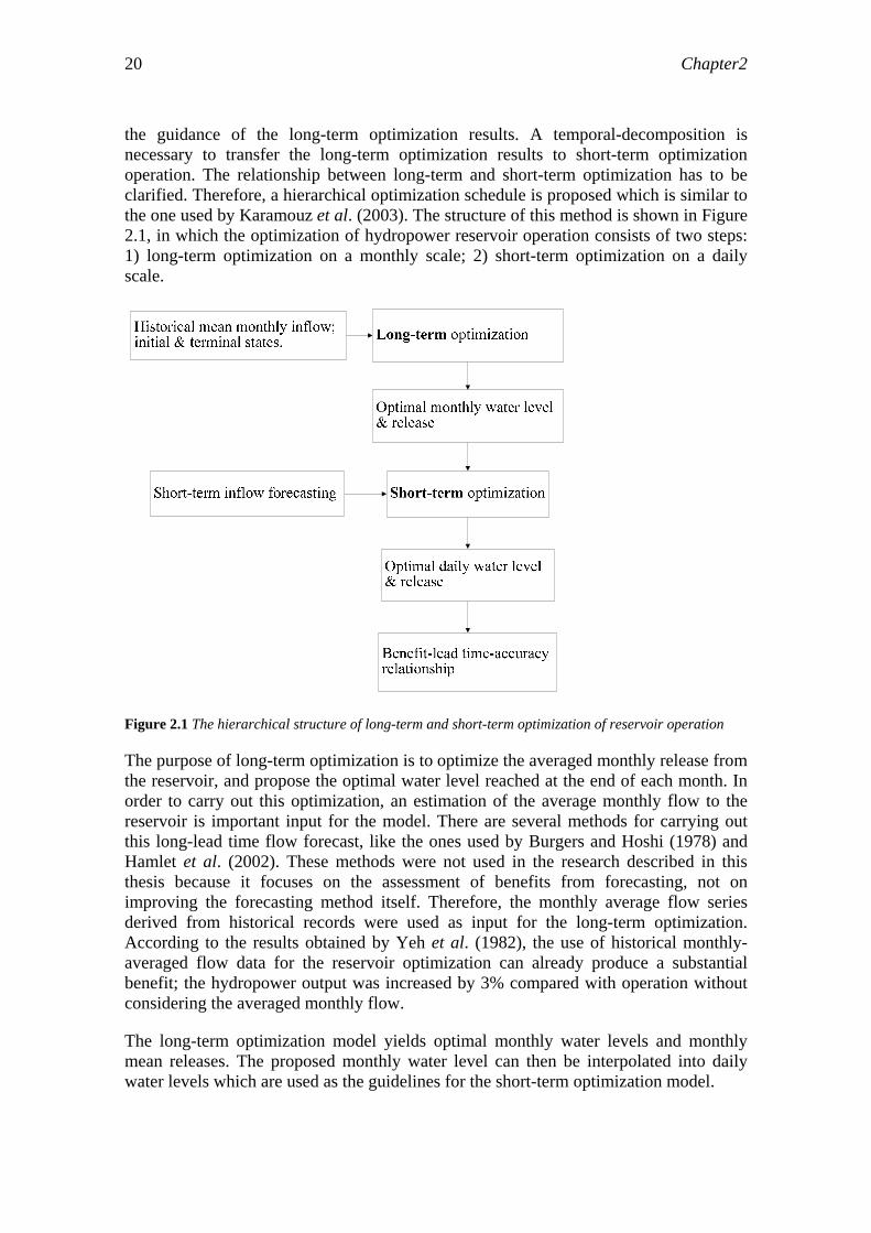
the guidance of the long-term optimization results. A temporal-decomposition is necessary to transfer the long-term optimization results to short-term optimization operation. The relationship between long-term and short-term optimization has to be clarified. Therefore, a hierarchical optimization schedule is proposed which is similar to the one used by Karamouz et al. (2003). The structure of this method is shown in Figure 2.1, in which the optimization of hydropower reservoir operation consists of two steps: 1) long-term optimization on a monthly scale; 2) short-term optimization on a daily scale.

Figure 2.1 The hierarchical structure of long-term and short-term optimization of reservoir operation

The purpose of long-term optimization is to optimize the averaged monthly release from the reservoir, and propose the optimal water level reached at the end of each month. In order to carry out this optimization, an estimation of the average monthly flow to the reservoir is important input for the model. There are several methods for carrying out this long-lead time flow forecast, like the ones used by Burgers and Hoshi (1978) and Hamlet et al. (2002). These methods were not used in the research described in this thesis because it focuses on the assessment of benefits from forecasting, not on improving the forecasting method itself. Therefore, the monthly average flow series derived from historical records were used as input for the long-term optimization. According to the results obtained by Yeh et al. (1982), the use of historical monthly-averaged flow data for the reservoir optimization can already produce a substantial benefit; the hydropower output was increased by 3% compared with operation without considering the averaged monthly flow.

The long-term optimization model yields optimal monthly water levels and monthly mean releases. The proposed monthly water level can then be interpolated into daily water levels which are used as the guidelines for the short-term optimization model.

Benefits of flow forecasting for reservoir operation 21

The short-term optimization model optimizes the daily reservoir release based on short-term flow forecasting, guided by the long-term optimization results. The resulting daily releases and water levels enable us to calculate the benefit obtained from short-term flow forecasting with different levels of forecasting capabilities (lead time and accuracies). A few representative lead times were selected to determine the relationship between benefit and lead time. The accuracy of the forecasting ranges from 40% of normalized deviation from the observed flows (ϕ , definition is given below) to zero, which implies a perfect forecasting of the flow series.

The synthesization of forecasted flow series considers the autocorrelation of the flows (De Kok et al., 2004):

1

'

−+=+=

tttt

ttt

QQQ

αβϕεδββ

(2.2)

'tQ is the synthesized flow at stage t; is the observed flow at stage t; tQ tβ is the noise

added to the observed flow series; tδ is a scaling factor drawn from a random uniform distribution in the interval [-1, +1]; ϕ is an assumed absolute deviation from ,

normalized with respect to , i.e., tQ

tQ ttt QQQ /' −=ϕ ; α is the autocorrelation

coefficient of the difference . The difference measures the accuracy of the forecasting at time t. The coefficient

tt QQ −'tt QQ −'

α is included to represent the fact that the forecasting error at a certain time is not completely random. It is partly related to the error in the forecast of the previous time step. As a rule of thumb (De Kok et al., 2004),

αϕ + is less than 1. Compared with the method used by Yeh et al. (1980, 1982), in which the forecasting errors were introduced into the synthesized flow series simply by adding random noise to the observed flow series, this flow synthesization model considers the autocorrelation of the successive forecasting errors: . Therefore, the resulting artificial flow series are closer to the real situation.

tt QQ −'

The assumed absolute deviation ϕ is an index of the local deviation from the observed discharge, which was used to generate the hypothetic forecasted flow series. However, ϕ is not the appropriate indicator to quantify the forecasting accuracy because it is the deviation of the individual forecasted flow with regard to the observed flow. A universal indicator for forecasting errors is necessary to measure the forecasting accuracies. The commonly used Nash-Sutcliffe coefficient (R2), originally proposed by Nash and Sutcliffe (1970), was adopted here. Once the forecasted series are synthesized by using Equation 2.2, their R2 values can be calculated. Next, the synthesized forecasting series can be used as input for the short-term optimization model to calculate the benefits.

Figure 2.2 shows the coupling of the long-term and short-term optimization models. Figure 2.2(a) presents the monthly water levels optimized from the long-term DDDP model and the actual water levels optimized by the coupled long-term and short-term DDDP models. Figure 2.2(b) is zoomed in from Figure 2.2(a) which demonstrates how this coupling works. At stage t=1, the initial state Hinit(1) is the actual water level at the beginning of a hydrological year (the first of May). If the lead time of the short-term flow forecasting is set to Tl, the terminal state of the first cycle of the short-term

Chapter2 22

optimization (Hterm(1)) is picked up from the long-term optimization results at stage Tl. Then the forecasted flow series is introduced into the short-term optimization model, and the optimal releases and water levels from stage 1 to stage Tl are calculated. Only the proposed optimal release of the first stage is used to calculate the actual water level at the end of the first stage based on the real flow ( ). The actual water level at the end of the first stage will be different from the water level obtained from the long-term optimization. The benefit obtained from the operation during the first stage can be calculated based on the optimal releasing policy and the actual water levels at the beginning and at the end of the stage. The actual water level at the end of the first stage is also the initial state of the second optimization cycle, which is marked as Hinit(2) in Figure 2.2(b). The optimization cycle will proceed iteratively to the end of the optimization horizon: one hydrological year (from the first of May to the end of April of the following year).

tQ

For each optimization cycle, the initial state is the actual water level, and the terminal water level is the water level interpolated from the monthly optimization result. This implies that after the operation of one optimization cycle, the water level should be able to fall back to the water level proposed by the long-term optimization model. This way, the results of the long-term optimization model form the basis and guidelines for the short-term optimization model, and both long-term and short-term benefits are considered simultaneously.

Benefits of flow forecasting for reservoir operation 23

50 100 150 200 250 300 350160

180

200

day

wat

er le

vel (

m)

(a)

water levels from long-term DDP model: Hterm(t)actual water level trajectory: Hinit(t)

Figure 2.2 The coupling of long-term and short-term optimization models. Hinit(t) are actual water levels which also serve as the initial conditions of every short-term optimization cycle; Hterm(t) are long-term optimization results, interpolated into daily water levels, serving as terminal conditions for each short-term optimization cycle.

2.3 Implementation

2.3.1 Description of the case study reservoir The Geheyan Reservoir used for applying the methodology proposed in the previous section is located on one of the tributaries of the Changjiang River (Yangtze): the Qingjiang River. Its geographic location in China is shown in Figure 2.3.

Chapter2 24

Figure 2.3 The geographic location of Qingjiang River basin and the Geheyan Reservoir (the tail of the reservoir reaches Yuxiakou)

The Geheyan Reservoir is a comprehensive multipurpose water resources development project planned to utilize potential benefits for hydropower, flood defence, navigation and so on, with hydropower generation as its main purpose. The reservoir started storing water on 10 April 1993 and on 30 November 1994, all four generators started generating electricity. Table 2.1 (QHDC and CWRC, 1998) lists the main features of the catchment area upstream of the reservoir, the reservoir itself, and the power plant. Figure 2.4 shows the major characteristic water levels and storage zones of the Geheyan Reservoir.

Benefits of flow forecasting for reservoir operation 25

Table 2.1 Principal features of the catchment, the Geheyan Reservoir and power plant

Characteristics Unit Value Catchment catchment area Km2 14430 average annual flow volume 109 m3 12.65 average annual precipitation mm 1400 average annual discharge at the dam site m3/s 400 Reservoir dam crest m 206 normal pool level (HN) m 200 spillway crest m 181.8 dead water level (HD) m 160 minimum elevation of foundation m 55 total storage (ST) 109 m3 3.431 flood control storage (SFC) 109 m3 0.72 beneficial storage (SB) 109 m3 1.975 effective storage (SE) 109 m3 2.286 reservoir capacity factor * % 15.6 Power plant average head m 108.9 maximum head m 121.4 minimum head m 80.7 maximum discharge through one turbine m3/s 325 number of power units 4 total installed capacity MW (Megawatt) 1200 firm output MW 180 average annual power output kWh 30.4

* Reservoir capacity factor = beneficial storage / average annual flow.

(206 m) dam crest(204.4 m) pool level during check flood(200 m) normal pool level(192.2 m) flood control level (1 May)

(181.8 m) spillway crest

(160 m) dead water level

(147.25 m) central line of intake tunnel

(74 m) central line of turbines

(55 m) minimum elevation of foundation

∨

∨ ∨

∧

∧

∧be

nefic

ial s

tora

ge(1

.975

×109 m

3 )de

ad s

tora

ge(1

.145

×109 m

3 )

tota

l sto

rage

(3.4

31×1

09 m3 )

Figure 2.4 Characteristics water levels and storage zones of the Geheyan Reservoir

Chapter2 26

The Qingjiang River is a mountainous river, with steep slopes flanking the stream. The valley is 200 to 1000 metres deep and forms a canyon-type reservoir, the length of which is about 90 km. However, the surface average area is only 55 km2. Figure 2.5 shows the elevation-storage relationship. The relationship between the release to downstream and the tail water level is important for calculating the generated electricity. Figure 2.6 presents the relationship between tail water level and release.

160 170 180 190 200

1.5

2

2.5

3

3.5

pool level (m) (above sea level)

wat

er s

tora

ge ( ×

109 m

3 )

Figure 2.5 Storage-pool level relationship of Geheyan Reservoir

80 85 90 95 1000

0.5

1

1.5

2

x 104

tail water level (m) (above sea level)

rele

ase

to d

owns

tream

(m3 /s

)

Figure 2.6 Relationship between release and tail water level of Geheyan Reservoir

Benefits of flow forecasting for reservoir operation 27

Rainfall in the Qingjiang River basin is very seasonal. Usually, the rain season extends from May to October and most big flooding events take place during this period. Therefore, the local water authority defined the first of May as the start of the hydrological year. Ideally, the reservoir is depleted from the beginning of the dry season (the first of November) to the dead-water level (the minimum endurable water level of the reservoir under normal hydrological and operational conditions) before the first of May, and from then on, refilled to the normal pool level at the end of the flooding season.

2.3.2 Deterministic dynamic programming models for a single reservoir operation

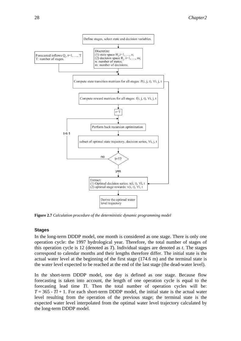
Calculation procedure of the model The structure of the DDDP model is defined by stages, states, decision variables, an objective function, constraints, and a recursive equation (their definitions are given in the following paragraphs). Optimal operation policies are obtained by iterating the recursive equation for each stage in one operation cycle. Here, the data of the 1997 hydrological year (from the first of May 1997 to the end of April 1998) are defined as one operation cycle and applied to demonstrate the methodology. The initial state of this operation cycle is the actual water level at the beginning of this hydrological year – 174.6 m – and the terminal state is the dead-water level (160 m). The Geheyan Reservoir is designed for intra-annual regulation. According to its regulation rules, the water level of the reservoir should fall back to the dead-water level at the end of a hydrological year, to make full use of the beneficial storage capacity of the reservoir. Figure 2.7 illustrates the calculation procedure of the DDDP model. The following subsections explain the steps used in the calculation procedure.

Chapter2 28

Figure 2.7 Calculation procedure of the deterministic dynamic programming model

Stages In the long-term DDDP model, one month is considered as one stage. There is only one operation cycle: the 1997 hydrological year. Therefore, the total number of stages of this operation cycle is 12 (denoted as T). Individual stages are denoted as t. The stages correspond to calendar months and their lengths therefore differ. The initial state is the actual water level at the beginning of the first stage (174.6 m) and the terminal state is the water level expected to be reached at the end of the last stage (the dead-water level).

In the short-term DDDP model, one day is defined as one stage. Because flow forecasting is taken into account, the length of one operation cycle is equal to the forecasting lead time Tl. Then the total number of operation cycles will be: T = 365 - Tl + 1. For each short-term DDDP model, the initial state is the actual water level resulting from the operation of the previous stage; the terminal state is the expected water level interpolated from the optimal water level trajectory calculated by the long-term DDDP model.

Benefits of flow forecasting for reservoir operation 29

State and decision variables The water level in the reservoir at the beginning of stage t is defined as the state of the system, for it is a natural index of marking the changes of the reservoir conditions. The total release during stage t is defined as the only decision variable, as it is the most influential way through which the reservoir operators can change the reservoir conditions. The definitions of the state and decision variables are the same for both short-term and long-term models.

tH

tR

Discretization of state and decision variables The water level between the normal pool level (200 m) and dead-water level (160 m) is taken as the space of the state. The normal pool level is the maximum elevation to which the reservoir surface will rise during ordinary operation conditions (Linsley et al., 1992). The pool level can be temporarily higher than the normal pool level during big flooding events. A higher than normal pool level is not the favourite state for reservoir operation. Keeping the water level higher than the normal pool level may lead to damage to the spillway gates. Therefore, the normal pool level is defined as the maximum feasible state of the operation. The storage volume difference between the normal pool level and dead-water level is defined as the beneficial storage ( ). The state space is equally divided into states spaced at 0.08 meter’s intervals. The total of the discretized states forms the feasible state space, which is denoted as S

3910975.1 m×

space.

The range of release volumes is also divided into equally spaced intervals. This range is from the minimum up to the maximum allowable downstream water release, constrained either by flood defence requirements, hydro-turbine discharge limits, and other factors. The total of the discretized decisions forms the feasible decision space, and is denoted as Rspace.

State transformation equation The state transformation equation is formulated according to the water balance: the storage at the end of one stage is equal to the initial storage at the beginning of the stage augmented with the stage's flow volume and minus the total released volume during the stage. It is expressed by the following equation:

tRQSS tttt ∆×−+=+ )(1 (2.3)

where is the reservoir storage at the beginning of stage t (mtS 3). It is derived from the water level and the storage-pool level relationship as shown in Figure 2.4. is the forecasted flow to the reservoir during stage t (m

tQ3/s). is the total release from the

reservoir during stage t (mtR

3/s). is the length of the stage. For the short-term DDDP models . For the long-term DDDP models, it varies depending on the stage (month). In this case, is equal to the number of days of the month multiplied by .

t∆st 41064.8 ×=∆

t∆s41064.8 ×

Chapter2 30

The state transformation relationship at one stage is stored as a two-dimensional matrix. The combination of all the two-dimensional state transformation matrices forms a three-dimensional state transformation matrix, denoted as P. The individual elements of the matrix are denoted as TtmjniwhereP tji ...,,2,1;...,,2,1;...,,2,1,,,, === , which means at stage t, starting with state i, after the implementation of decision j, the state will reach the value saved in . The constants n, m and T are the total number of states, decisions and stages respectively.

tjiP ,,

Physical constraints of the reservoir The spaces of the states and the decisions are limited by the physical conditions of the reservoir and the up- and down-stream areas. The following three types of constraints should be considered in the reservoir optimal operation:

(1) The storage-water level relationship:

tHfS tSHt ∀= ),( (2.4)

where is the reservoir storage-water level relationship shown in Figure 2.4. )(HfSH

(2) Maximum release ( ) defined by flood defence requirements and minimum release ( ) required by navigation, irrigation, water supply, creation, fishing, wild life protection, etc.:

maxR

minR

tRRR t ∀≤≤ ,maxmin (2.5)

(3) Maximum ( ) and minimum ( ) discharge through the turbines: maxRe minRe

tt ∀≤≤ ,ReReRe maxmin (2.6)

The water level inside the reservoir is defined as the state variable. The state transformation is realized by calculating the total volume of the water flowing into or released from the reservoir. The above storage-water level relationship (2.4) is used for converting the water levels into corresponding storage volumes. After the application of the state transformation equation (Equation 2.3), the same relationship is used to convert the calculated storages back to corresponding water levels. The constraints introduced by Equation 2.5 and 2.6 are used to set the upper and lower limits of the feasible decision space (R

tt HS ~

space), where, , , , .

smR /150 3min = smR /13000 3

max =

sm /100Re 3min = sm /1300Re 3

max =

Objective function The objective of this reservoir is to generate maximum electricity with firm power equal to 180 MW under a design guarantee rate of 92%. The design guarantee rate of the power plant is the percentage of the time (92%), that the generated power has to be higher than 180 MW. The firm power is the average power output during dry season (i.e.

Benefits of flow forecasting for reservoir operation 31

a kind of minimum output). The values of firm power (180 MW) and design guarantee rate (92%) are stipulated by QHDC and CWRC (1998). In addition, the downstream flood control requirements have to be satisfied.

Therefore, the objective function can be formulized as:

( ) ( )[ ]tttt

T

ttftt

T

ttt

hHgE

EEHeEHBB

−=⎭⎬⎫

⎩⎨⎧

−⋅−=⎭⎬⎫

⎩⎨⎧

= ∑∑==

Re

maxmax11

max

η

ν (2.7)

where B is the same benefit function as given by Equation 2.1;

tft EEHe −ν is a penalty function embedded in the objective function to force the system to produce power greater than the firm power;

is electric energy produced during stage t; tE

ν is the penalty factor, ν = 0.4, the selection of this value is given in the next paragraph;

is a unit step function, ;

is the power output at stage t, kW;

is the firm power, ;

is the firm energy,

tHe ⎪⎩

⎪⎨⎧

<

≥=

ft

ftt NN

NNHe

,1

,0

tN

fN MWN f 180=

fE tNE ff ∆= ;

is the length of the stage;

g is the acceleration of gravity, ;

t∆

2/81.9 smg =

η is the acceleration the effici cy of the hydropower plant, 866.0321 =××en = ηηηη (Zhou et al. 997); where 1, 1 η is the efficiency of turbines; 2η is th efficiency of generators; 3

eη is the efficiency of transmission mechanisms; η is a varying

coefficient according to the net water head and the discharge through the turbine. Here a constant empirical value (0.866) is taken for such a large-scale hydropower plant (total installed capacity greater than 250 MW), according to the recommendation of Zhou et al. (1997).

is the release through turbines during stage t; tRe

tH is the average reservoir water level during stage t; and

Chapter2 32

th is the average tail-water level during stage t.

The flood control requirements are imposed in physical constraints stated in the previous subsection.

The choice for the value of the penalty factor ν will remarkably influence the final annual electricity output and the design guarantee rate. In order to determine the value of ν that leads to the required design guarantee rate (92%), an investigation of the influence of different values of ν on the resulting design guarantee rates was carried out. The flow forecasting is assum d to be perfect and the lead time is set to 4 days. The results are shown in Table 2.2 d indicate that

e an ν =0.4 is the correct value for the

Ta ce na cto e ltin r ra

penalty factor.

ble 2.2 The influen of pe lty fa r on th resu g gua antee te

ν 0.1 0.2 0.3 0.4 0.5 0.6 0.7 0.8 0.9 1 guarantee rate (%) 82.7 86.3 88.8 91.5 94.5 94.5 94.5 95.6 95.9 95.9

The recursive equation The backward recursive algorithm was used to find the optimal policies and the corresponding optimal states. The recursive equation is:

),,(

,,)},,,(),,({max),,( 1111

−⋅−=

∀∀∀+=

0),,( 1111 =++++ TTTT RQHB

All variables and parameters have the same meanings as in the previous equations. This recursive equation is applied iteratively from the final stage back until the first stage as shown in Figure 2.7. For each feasible state of an intermediate stage, one optimal sub-policy is memorized for the next backward optimization operation. The overall optimal policy is identified when the first stage is reached because only one state can exist (the actual water level from which the optimization cycle starts). The optimal state trajec

++++∈

tftttttt

tttttttttttRspaceRtttt

EEHeERQHb

RQHRQHBRQHbRQHBtt

ν (2.8)

tory (water level) and the maximum benefit can be consequently identified by applying the

the beginning to the end of the process.

nthly flow series are determined from the recorded monthly flow series from 1951 to 1990. They are shown in Figure 2.8, together with the corresponding standard deviations.

state transformation equation forward from

2.3.3 The data The monthly reservoir operation is optimized by using the long-term optimization model, based on the average monthly flow series. The average mo

Benefits of flow forecasting for reservoir operation 33

Figure 2.8 Average monthly discharge (solid symbols) and corresponding standard deviation (error bars) recorded at the dam site of Geheyan Reservoir

Figure 2.9 shows an example of one series of synthesized flow data for the short-term optimization, together with the original data. The statistics of both observed and synthesized series are given in Table 2.3. The mean and the lag-one autocorrelation coefficient of the observed series are duplicated closely by the method represented by Equation 2.2. The standard deviation increases slightly for increasing ϕ , which is understandable because a higher ϕ corresponds to more noise and thus a greater standard deviation.

0 10 20 30 40 50 600

500

1000

1500

2000

2500

3000

days

inflo

w (m

3 /s)

observed seriessynthesized: φ=0.1synthesized: φ=0.4

Figure 2.9 Observed and synthesized data with different levels of added noise: ϕ =0.1 and 0.4 (ϕ is the assumed absolute deviation from recorded discharge).

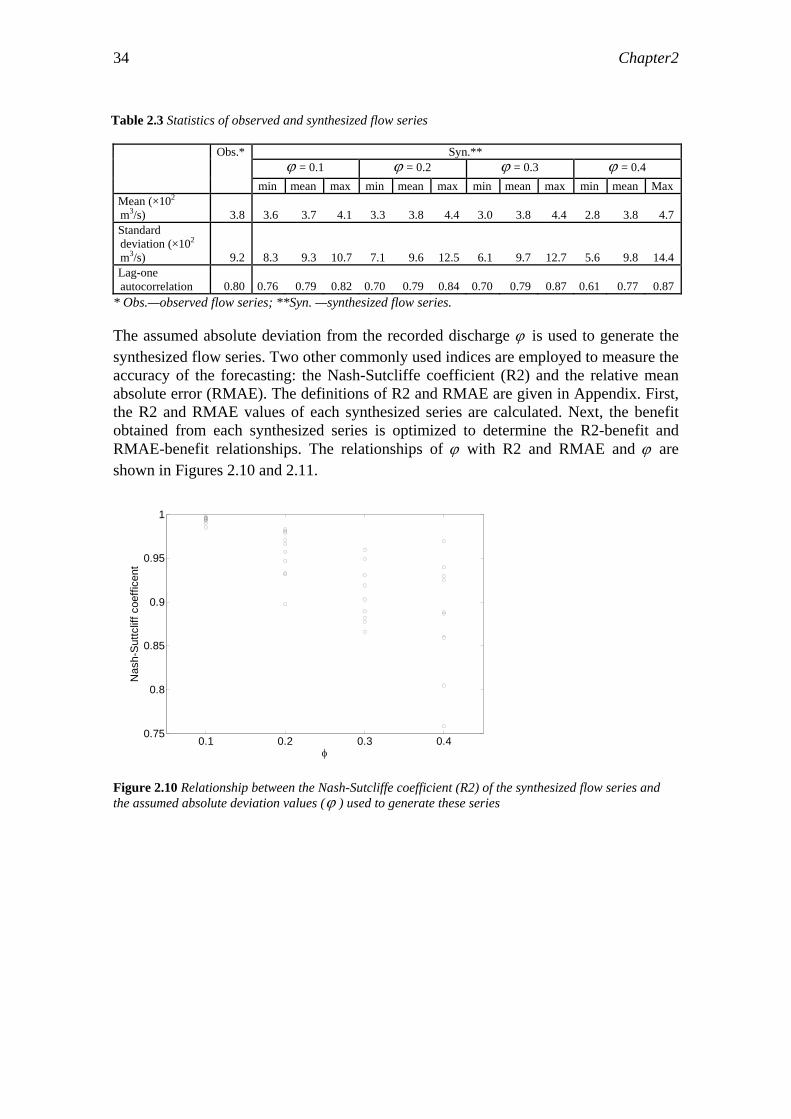
Chapter2 34

Table 2.3 Statistics of observed and synthesized flow series

Obs.* Syn.** ϕ = 0.1 ϕ = 0.2 ϕ = 0.3 ϕ = 0.4 min mean max min mean max min mean max min mean Max Mean (×102 m3/s) 3.8 3.6 3.7 4.1 3.3 3.8 4.4 3.0 3.8 4.4 2.8 3.8 4.7 Standard deviation (×102 m3/s) 9.2 8.3 9.3 10.7 7.1 9.6 12.5 6.1 9.7 12.7 5.6 9.8 14.4 Lag-one autocorrelation 0.80 0.76 0.79 0.82 0.70 0.79 0.84 0.70 0.79 0.87 0.61 0.77 0.87

* Obs.—observed flow series; **Syn. —synthesized flow series.

The assumed absolute deviation from the recorded discharge ϕ is used to generate the synthesized flow series. Two other commonly used indices are employed to measure the accuracy of the forecasting: the Nash-Sutcliffe coefficient (R2) and the relative mean absolute error (RMAE). The definitions of R2 and RMAE are given in Appendix. First, the R2 and RMAE values of each synthesized series are calculated. Next, the benefit obtained from each synthesized series is optimized to determine the R2-benefit and RMAE-benefit relationships. The relationships of ϕ with R2 and RMAE and ϕ are shown in Figures 2.10 and 2.11.

0.1 0.2 0.3 0.40.75

0.8

0.85

0.9

0.95

1

φ

Nas

h-S

uttc

liff c

oeffi

cent

Figure 2.10 Relationship between the Nash-Sutcliffe coefficient (R2) of the synthesized flow series and the assumed absolute deviation values (ϕ ) used to generate these series

Benefits of flow forecasting for reservoir operation 35

0.1 0.2 0.3 0.40.05

0.1

0.15

0.2

0.25

0.3

0.35

0.4

φ

rela

tive

mea

n ab

solu

te e

rror

Figure 2.11 Relationship between the Relative Mean Absolute Error (RMAE) of the synthesized flow series and the assumed absolute deviation values (ϕ ) used to generate these series

R2 defines the efficiency of a hydrological model. It ranges from minus infinity to one, with higher values indicating better agreement between forecasted and observed discharges. RMAE measures the relative absolute error of forecasted series. It ranges from zero to positive infinity, with lower values indicating better forecasting performance. It provides a different way of evaluating the forecasting accuracy, other than correlation-based measures like R2. Legates and McCabe (1999) recommended the simultaneous utilization of these two types of measures for evaluating flow forecasting performance. No in-depth analyses were made of these measures within the present research, for this was outside its scope. Both Figure 2.10 and Figure 2.11 indicate that higher ϕ values lead to a deterioration of the agreement between observed and forecasted (synthesized) series. This is understandable because higher ϕ values mean synthesized discharges with a higher probability of a greater deviation from the observed discharge.

2.4 Results and discussion

2.4.1 Benchmark and actual operation benefits The actual electricity generated during the hydrological year 1997 is 2.2×109 KWh according to the reports provided by the Reservoir Regulation Centre of the Qingjiang Hydropower Development Cooperation (QHDC and CWRC, 1998). In order to compare the benefits obtained from forecasts with varying levels of accuracy, a benchmark benefit needs to be set; it was defined as the benefit obtained from a perfect flow forecast 1 year ahead. It represents the theoretical maximum benefit that can be obtained from forecasting and optimization. In addition to the benchmark benefit, the benefits obtained from a perfect flow forecast with a lead time of 4 days and a lead time of 10 days are also studied, to deduce the effect of the lead time of flow forecasting on power benefit. The results are presented in Figure 2.12. Figure 2.12(a) shows the observed flow series of the Geheyan Reservoir in the 1997 hydrological year. The optimized release, water level and power output trajectories are presented in Figures 2.12(b), (c)

Chapter2 36

and (d), respectively. The optimal results for 10 and 4 days perfect flow forecasts were also calculated and are included in the corresponding sub-figures. In Figure 2.12(c), the monthly water levels proposed by the long-term optimization model are also presented.

As shown in Figure 2.12(a), there was only one large flooding event in the flooding season of the 1997 hydrological year. The maximum 72 hours’ flood is 2.32×109 m3, which corresponds to a flood with a frequency of occurrence of about 4% according to QHDC and CWRC (1998). There were two successive discharge peaks during this flooding event; the second started 2 days after the first.

Figure 2.12(b) presents the optimized releases from the reservoir. Releases less than 1300 m3/s (the maximum release via turbines) are released through the turbines to generate electricity. For releases higher than that, the surpluses are released through flood-releasing works (spill gates, spillways or bypass conduits). The total wasted volume can be calculated by integrating the releases through the flood-releasing works over time. The total wasted volumes under flow forecasts with a lead time of 1 year, 10 and 4 days are 0.8×109, 2.0×109 and 2.5×109 m3 respectively, corresponding to 6, 16 and 20% of the average annual flow volume (see Table 2.1). Therefore, for increasing lead times, the volume of water that will be spilled decreases. For the situation before the arrival of the flood of July 1997, flow forecasts with longer lead times resulted in earlier full-load operation of the generators, in order to generate more electricity by decreasing the volume of the spilled water.

This pre-releasing (before the arrival of the flood) can also be identified easily from Fig 2.11(c): for flow forecasts with longer lead times, the water level starts to decrease earlier, relative to the arrival of the flood event as a result of optimization. Another factor revealed by Figure 2.12(c) is that although the flood event in July 1997 lasted only 10 days, the reservoir needed to start depleting the storage about 30 days before the beginning of the flood in order to generate maximum electricity. However, if the major operational purpose of the reservoir were not power generation, but for instance flood defence, pre-releasing would be able to start much later because the releasing capacity of the flood sluices is much bigger than that of the turbines.

Figure 2.12(d) shows the optimized power output in the hydrological year 1997. Table 2.4 lists the corresponding total benefits (in term of electricity generated) as well as the benefit obtained from the actual operation. As shown in Table 2.4, the benchmark benefit (3.0×109 kWh) is 35% higher than the actually obtained benefit (2.2×109 kWh). Perfect flow forecasts with a lead time of 10 days and 4 days can realize 93% and 87% of the maximum benefit respectively.

Table 2.4 Expected benefits under perfect flow forecasting and actual benefit obtained from real operation.

Lead time (days) Benefits (×109 kWh) % of benchmark benefit 365 3.0 100 10 2.8 93 Perfect flow forecasts 4 2.6 87

Actual operation unclear 2.2 73

Benefits of flow forecasting for reservoir operation 37

According to Fig 2.11(c), because of the flood event in July, the reservoir started to pre-release the storage prior to the arrival of the flood. In order to identify when pre-releasing the storage has to start, the optimization results during, before and after the flood event are sampled from Fig 2.11, enlarged and displayed in Fig 2.12. The sampling duration is from 11 June to 26 July 1997.

According to Fig 2.12(c), in order to maximize the benefit, the reservoir operation related to the flood event consists of two successive stages: pre-releasing and refilling. The refilling always starts (or the pre-releasing always ends) at the beginning of the flood event: 14 July, to make maximum use of the flooding water. From that time, the refilling will continue until the maximum water level is reached. The duration of the refilling depends on the volume emptied by the pre-releasing operation. Notice that, for flow forecasts with a lead time equal to 4 and 10 days, the refilling durations are 2 days shorter (from 14/7 to 16/7) than when the lead time of the flow forecast is 1 year (from 14/7 to 18/7). The duration of the pre-releasing increases for increasing lead times of flow forecast: 2 and 8 days for forecast lead times of 4 and 10 days respectively. For flow forecasting with a lead time of 4 and 10 days, the total duration of the pre-releasing and refilling periods (Td) is equal to the lead time.

For lead times smaller than 33 days (the threshold lead time; this will be explained immediately below), Td increases with the increase of Tl, and Td= Tl. However, Figure 2.13 (c) shows that it will not always increase with the increase of Tl. For Tl equal to 1 year, Td is 33 days (the water level starts to decrease on 15 June, and fills up again on 18 July). It is anticipated that for Tl greater than 33 days, Td will not be more than 33 days, because the dead-water level has already been reached: no more space can be made available under forecasts with longer lead times. Therefore, 33 days is identified as the maximum Td. Also, it is the maximum required lead time of the flow forecast (Tl) in order to reach the maximum (benchmark) benefit. Therefore, it is denoted as the threshold lead time (Tlthreshold). Further extension of the forecasting lead time beyond Tlthreshold will not lead to a significant increase in benefit. Although a lead time of 33 days is not realistic, the Tlthreshold gives the upper limit of an appropriate flow forecasting in terms of lead time. The value of the threshold lead time depends on:

(1) the physical features of the reservoir, such as the storage volume and the releasing capacity of the turbines and the flood-releasing works; and

(2) the character of the impending flooding events: larger flooding events (either larger volumes or higher peak discharges) will lead to longer threshold lead times.

As a lead time of 33 days is infeasible in reality, the feasible lead time of a flow forecasting can be determined by calculating the hydrological response time of the basin. In this case, it solely depends on the hydrological conditions of the river basin. In order to investigate the influence of the forecasting accuracies on the benefits, a feasible lead time of 4 days (1 day hydrological response time plus 3 days rainfall forecast) will be chosen to simulate the benefits.

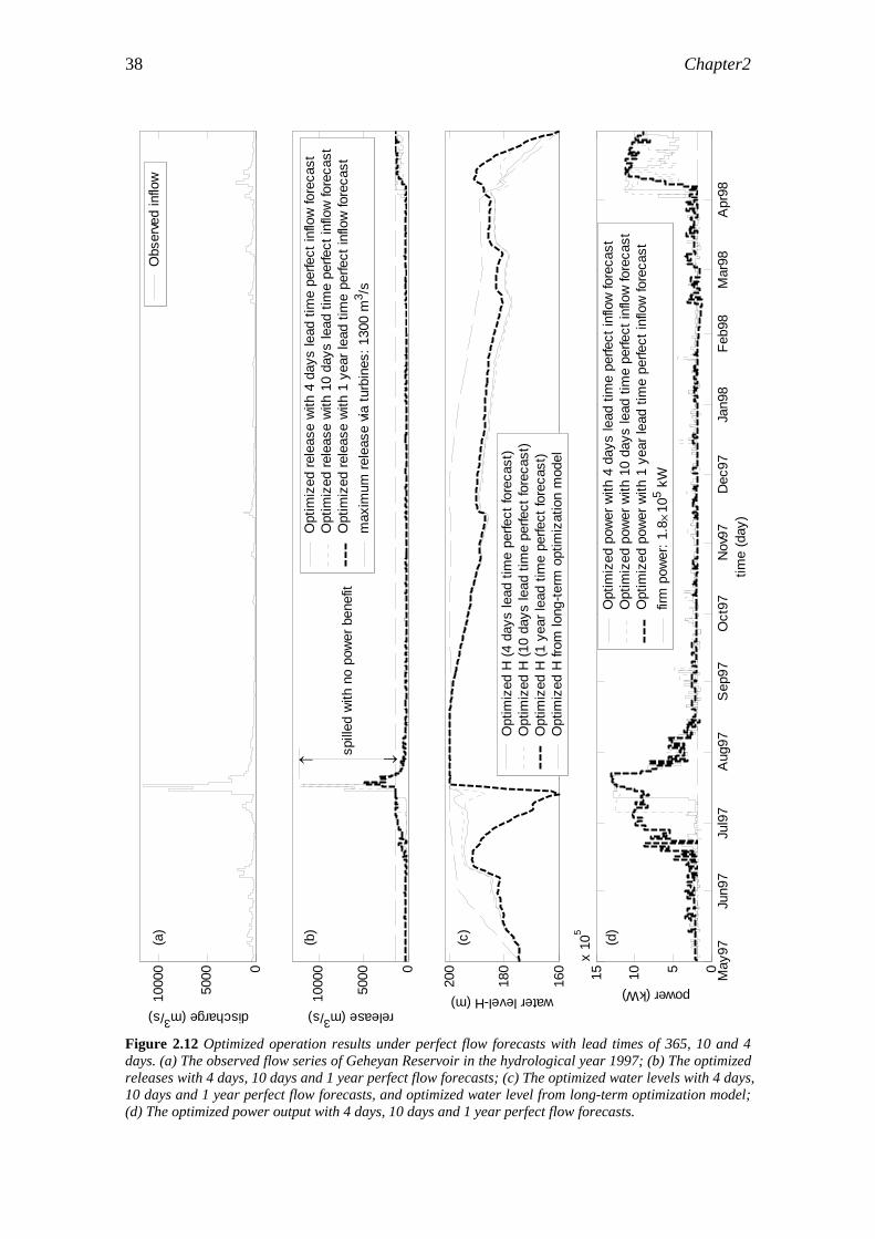
Chapter2 38

Figure 2.12 Optimized operation results under perfect flow forecasts with lead times of 365, 10 and 4 days. (a) The observed flow series of Geheyan Reservoir in the hydrological year 1997; (b) The optimized releases with 4 days, 10 days and 1 year perfect flow forecasts; (c) The optimized water levels with 4 days, 10 days and 1 year perfect flow forecasts, and optimized water level from long-term optimization model; (d) The optimized power output with 4 days, 10 days and 1 year perfect flow forecasts.

0

5000

1000

0

discharge (m3/s)

(a)

Obs

erve

d in

flow

0

5000

1000

0

release (m3/s)

(b)

↑ ↓spill

ed w

ith n

o po

wer

ben

efit

Opt

imiz

ed re

leas

e w

ith 4

day

s le

ad ti

me

perfe

ct in

flow

fore

cast

Opt

imiz

ed re

leas

e w

ith 1

0 da

ys le

ad ti

me

perfe

ct in

flow

fore

cast

Opt

imiz

ed re

leas

e w

ith 1

yea

r lea

d tim

e pe

rfect

inflo

w fo

reca

stm

axim

um re

leas

e via

turb

ines

: 130

0 m

3 /s

160

180

200

water level-H (m)

(c)

Opt

imiz

ed H

(4 d

ays

lead

tim

e pe

rfect

fore

cast

)O

ptim

ized

H (1

0 da

ys le

ad ti

me

perfe

ct fo

reca

st)

Opt

imiz

ed H

(1 y

ear l

ead

time

perfe

ct fo

reca

st)

Opt

imiz

ed H

from

long

-term

opt

imiz

atio

n m

odel

May

97Ju

n97

Jul9

7A

ug97

Sep

97O

ct97

Nov

97D

ec97

Jan9

8Fe

b98

Mar

98A

pr98

051015x

105

power (kW)

time

(day

)

(d)

Opt

imiz

ed p

ower

with

4 d

ays

lead

tim

e pe

rfect

inflo

w fo

reca

stO

ptim

ized

pow

er w

ith 1

0 da

ys le

ad ti

me

perfe

ct in

flow

fore

cast

Opt

imiz

ed p

ower

with

1 y

ear l

ead

time

perfe

ct in

flow

fore

cast

firm

pow

er: 1

.8×1

05 kW

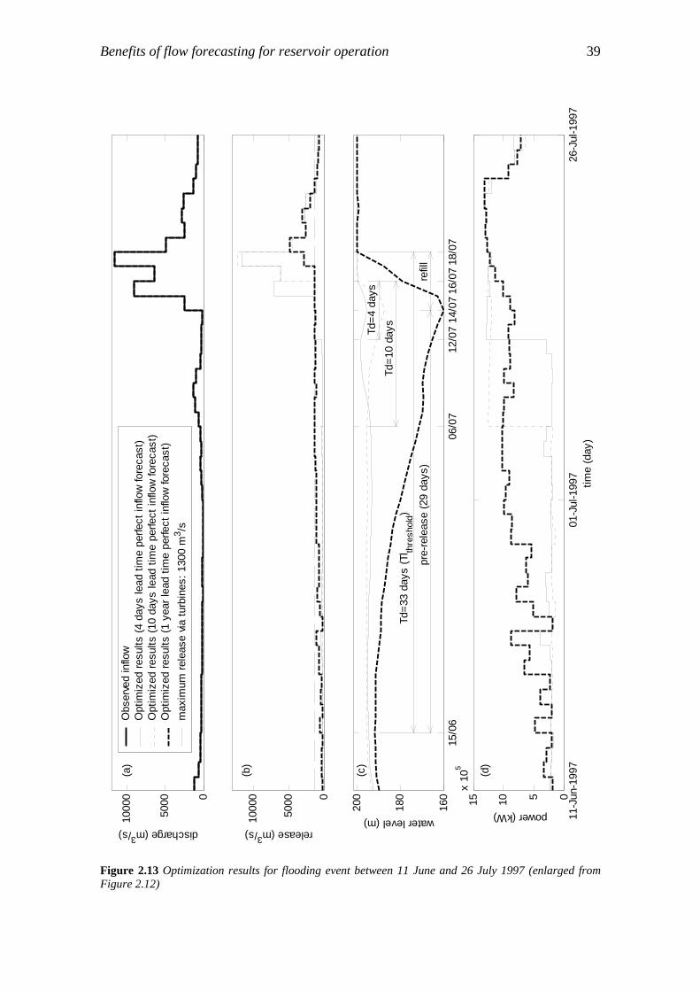
Benefits of flow forecasting for reservoir operation 39

0

5000

1000

0

discharge (m3/s)

(a)

Obs

erve

d in

flow

Opt

imiz

ed re

sults

(4 d

ays

lead

tim

e pe

rfect

inflo

w fo

reca

st)

Opt

imiz

ed re

sults

(10

days

lead

tim

e pe

rfect

inflo

w fo

reca

st)

Opt

imiz

ed re

sults

(1 y

ear l

ead

time

perfe

ct in

flow

fore

cast

)m

axim

um re

leas

e via

turb

ines

: 130

0 m

3 /s

0

5000

1000

0

release (m3/s)

(b)

15/0

606

/07

12/0

714

/07

16/0

718

/07

160

180

200

water level (m)

Td=1

0 da

ysTd=4

day

s

Td=3

3 da

ys (T

l thre

shol

d)

pre-

rele

ase

(29

days

)re

fill

(c)

11-J

un-1

997

01-J

ul-1

997

26-J

ul-1

997

051015x

105

power (kW)

time

(day

)

(d)

Figure 2.13 Optimization results for flooding event between 11 June and 26 July 1997 (enlarged from Figure 2.12)

Chapter2 40

2.4.2 Benefits obtained from flow forecasting with different accuracies Figures 2.14 and 2.15 present the optimized benefits calculated from the synthesized flow series with different forecasting accuracies. The lead time of the forecasting is fixed at 4 days to illustrate the implementation of the method. In these two figures, the trends of electricity – forecasting performances are illuminated by adding curves fitted to the data pairs. A linear equation is used for both figures. As can be seen from these two figures, the benefits increase generally with increasing model performances (either in R2 or in RMAE terms). In order to prove that there exists an increasing (or decreasing) trend in the data presented in Figures 2.14 and 2.15, a mean line (the dashed lines), which represents the mean value of the benefits, is added to both figures. The Mean Squared Errors (MSE) of both fitted lines (solid lines) and mean lines (dashed lines) with respect to the data (the dots) are calculated to shown their goodness-of-fit to the data. The definition of MSE is given in Appendix. The MSE values are shown in both figures. As can be seen, the MSE values for the fitted lines in both figures are higher than the MSE values for the mean lines. This means that the solid lines fit the data better than the dashed lines. This proves that the increasing or decreasing trends discovered in Figures 2.14 and 2.15 by the fitted curves are correct. This way of detecting the existence of the trend in a data set implies a hypothesis that, if the MSE of the fitted line is smaller than the MSE of the mean line, there is always a trend. Further research on testing the truth of this hypothesis may be necessary. It can be intuitively known at the moment that, the truth of this hypothesis relates to the number of data pairs, and the significance level pre-determined for this hypothesis test.

The actual total electricity generated from the real operation is 2.2×109 kWh. According to the fitted curves in Figures 2.13 and 2.14, any 4-day ahead flow forecasting with R2 greater than 0.70 (or RMAE less than 0.40) can at least obtain electricity of 2.31×109 KWh, an increase of 5% compared to the actual operation. If we assume an R2 value of 0.90 (or an RMAE value of 0.25) to be feasible for a 4-day ahead flow forecasting, then electricity of 2.40×109 KWh can be obtained, an increase of 9% compared to the actual operation. Thus, the benefit can vary from 5% to 9% increase compared with the real operation benefit.

Figures 2.14 and 2.15 also indicate that high-accuracy flow forecasts do not always lead to large benefits. The relationships between benefit and forecasting accuracies are quite dispersed. This scatter of the data points can be explained by the following three reasons:

(1) A sub-optimal decision (because of mis-estimation of the flow) made at a certain stage will yield losses in the future. For example, an overestimation of the flow at the end of a flood season will lead to the decision to lower the water level. Because of a lack of flow water during the following dry season, the water level will remain low for a long period, during which the power output will be lower. This effect will be smaller in the flooding season, because the extra released volume can be easily replaced by abundant flooding water in the flooding season. Because of the randomness in generating the forecasting errors for the synthesized flow series, the chance of over-depletion of the storage and the long-term consequences of benefit losses are also random. Therefore, even if the overall R2 values of flow forecasts are satisfactory, the variation in the benefits are still high.

Benefits of flow forecasting for reservoir operation 41

(2) Both R2 and RMAE are criteria designed for measuring the difference between the forecasted and observed flow series (forecasting errors), not for measuring the increased electricity obtained from better flow forecasting. As seen from Equation 2.7, the forecasting errors do not play an explicit role in determining the amount of electricity generated. Their influence on benefit will have to be taken in consideration through reservoir operation practices and will either depress or enhance the benefit to some degree (a random process, as explained). A new, more effective measure of flow forecasting accuracy for improving power generation may be more appropriate for identifying this benefit-forecasting accuracy relationship.

(3) Flow forecasting is not the only factor which has a fundamental influence on the improvement of power generation; the operation strategies also play an important role. The question which one (forecasting or operation) dominates remains a problem to be solved.

An appropriately accurate flow forecast can be defined as a forecast that leads to a certain benefit, expressed as a percentage of the benchmark, the theoretical maximum benefit. For example, if a benefit of 80% of the benchmark benefit (which is 2.40×109 kWh) is required, a flow forecasting with accuracy in terms of an R2 value of 0.88 is necessary. The choice for the criterion depends not only on the reservoir operator’s preference, but also on the physical reality of the studied river basin. In general, a basin with a larger area, a longer river channel and more stable climate conditions generally leads to more reliable flow forecasting.

MSE = 2.15E+15

MSE = 2.63E+15

2.30E+09

2.35E+09

2.40E+09

2.45E+09

2.50E+09

2.55E+09

0.7 0.75 0.8 0.85 0.9 0.95 1

R2

tota

l ele

ctri

city

gen

erat

ed (k

Wh)

Figure 2.14 The relationship between the benefits and the Nash-Sutcliffe coefficient of the forecasted flow series. The straight line is the line fitted to the data (dots) by using a linear equation; the dashed line represents the mean of the data; The MSEs attached are the Mean Squared Errors of these two lines to the data.

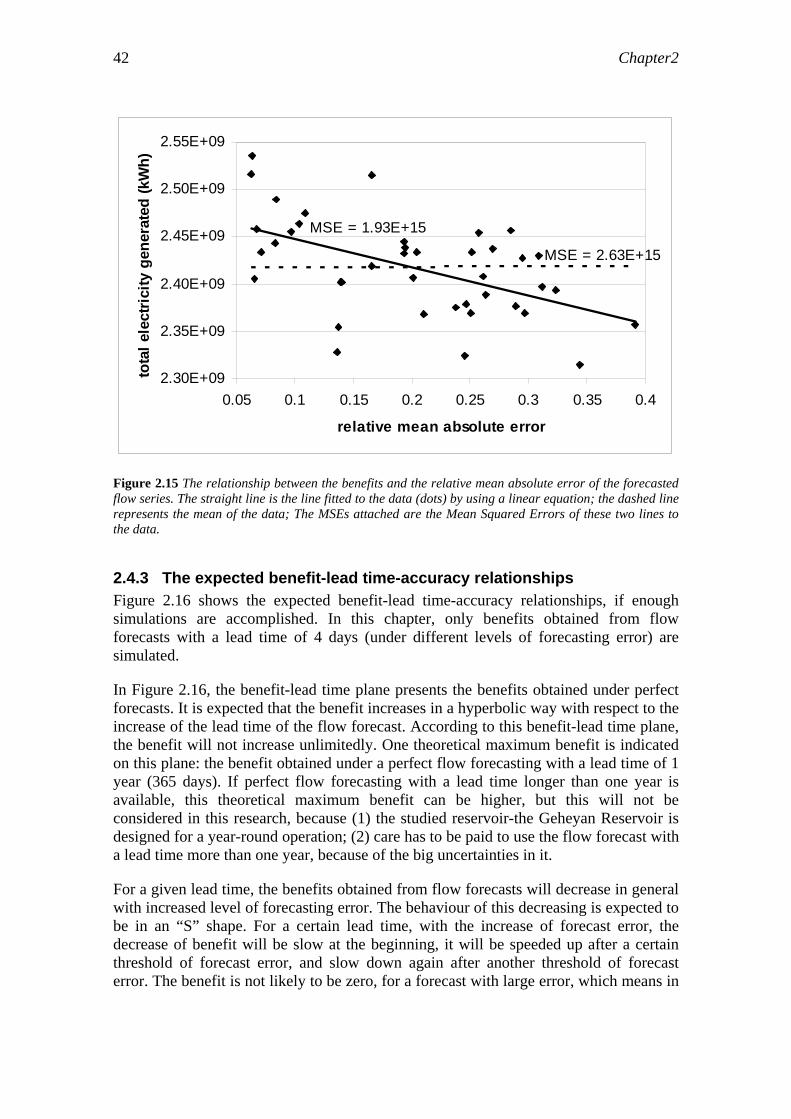
Chapter2 42

MSE = 1.93E+15

MSE = 2.63E+15

2.30E+09

2.35E+09

2.40E+09

2.45E+09

2.50E+09

2.55E+09

0.05 0.1 0.15 0.2 0.25 0.3 0.35 0.4

relative mean absolute error

tota

l ele

ctri

city

gen

erat

ed (k

Wh)

Figure 2.15 The relationship between the benefits and the relative mean absolute error of the forecasted flow series. The straight line is the line fitted to the data (dots) by using a linear equation; the dashed line represents the mean of the data; The MSEs attached are the Mean Squared Errors of these two lines to the data.

2.4.3 The expected benefit-lead time-accuracy relationships Figure 2.16 shows the expected benefit-lead time-accuracy relationships, if enough simulations are accomplished. In this chapter, only benefits obtained from flow forecasts with a lead time of 4 days (under different levels of forecasting error) are simulated.

In Figure 2.16, the benefit-lead time plane presents the benefits obtained under perfect forecasts. It is expected that the benefit increases in a hyperbolic way with respect to the increase of the lead time of the flow forecast. According to this benefit-lead time plane, the benefit will not increase unlimitedly. One theoretical maximum benefit is indicated on this plane: the benefit obtained under a perfect flow forecasting with a lead time of 1 year (365 days). If perfect flow forecasting with a lead time longer than one year is available, this theoretical maximum benefit can be higher, but this will not be considered in this research, because (1) the studied reservoir-the Geheyan Reservoir is designed for a year-round operation; (2) care has to be paid to use the flow forecast with a lead time more than one year, because of the big uncertainties in it.

For a given lead time, the benefits obtained from flow forecasts will decrease in general with increased level of forecasting error. The behaviour of this decreasing is expected to be in an “S” shape. For a certain lead time, with the increase of forecast error, the decrease of benefit will be slow at the beginning, it will be speeded up after a certain threshold of forecast error, and slow down again after another threshold of forecast error. The benefit is not likely to be zero, for a forecast with large error, which means in

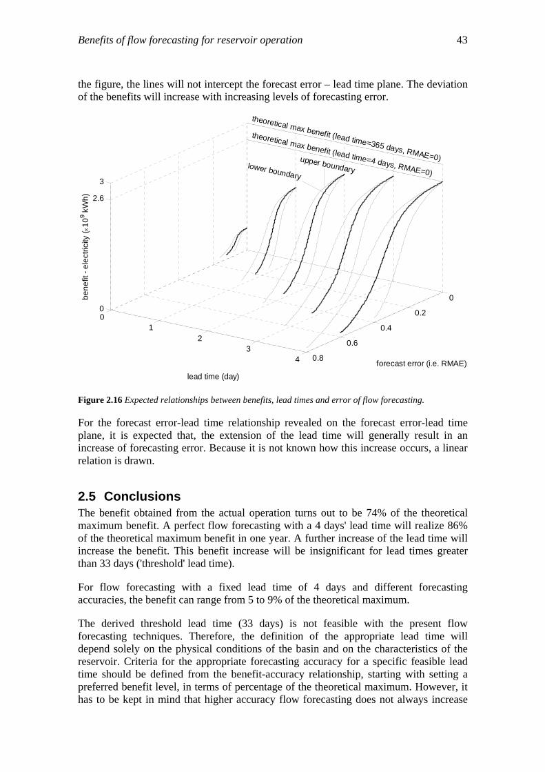
Benefits of flow forecasting for reservoir operation 43

the figure, the lines will not intercept the forecast error – lead time plane. The deviation of the benefits will increase with increasing levels of forecasting error.

01

23

4 0.8

0.6

0.4

0.2

00

2.6

3

forecast error (i.e. RMAE)

upper boundary

theoretical max benefit (lead time=4 days, RMAE=0)

theoretical max benefit (lead time=365 days, RMAE=0)lower boundary

lead time (day)

bene

fit -

elec

trici

ty ( ×

109 k

Wh)

Figure 2.16 Expected relationships between benefits, lead times and error of flow forecasting.

For the forecast error-lead time relationship revealed on the forecast error-lead time plane, it is expected that, the extension of the lead time will generally result in an increase of forecasting error. Because it is not known how this increase occurs, a linear relation is drawn.

2.5 Conclusions The benefit obtained from the actual operation turns out to be 74% of the theoretical maximum benefit. A perfect flow forecasting with a 4 days' lead time will realize 86% of the theoretical maximum benefit in one year. A further increase of the lead time will increase the benefit. This benefit increase will be insignificant for lead times greater than 33 days ('threshold' lead time).

For flow forecasting with a fixed lead time of 4 days and different forecasting accuracies, the benefit can range from 5 to 9% of the theoretical maximum.

The derived threshold lead time (33 days) is not feasible with the present flow forecasting techniques. Therefore, the definition of the appropriate lead time will depend solely on the physical conditions of the basin and on the characteristics of the reservoir. Criteria for the appropriate forecasting accuracy for a specific feasible lead time should be defined from the benefit-accuracy relationship, starting with setting a preferred benefit level, in terms of percentage of the theoretical maximum. However, it has to be kept in mind that higher accuracy flow forecasting does not always increase

Chapter2 44

the benefit (this can be observed form the scattering of the benefit values presented in Figure 2.14 and 2.15), although in general it does. The obtained benefit also depends on the operation strategies of the reservoir. The effect of the interaction between the flow forecasting and the reservoir operation strategies on the benefit needs to be further explored.

This chapter has been published as: Dong, X., Dohmen-Janssen, C.M. and Booij, M.J., 2005. Appropriate spatial sampling of rainfall for flow simulation. Hydrological Sciences Journal, 50(2), 279-298.

Chapter 3

Appropriate spatial sampling of rainfall for flow simulation

Abstract The objective of this chapter is to find the appropriate number and location of raingauges for a river basin for flow simulation by using statistical analyses and hydrological modelling. First, a statistical method is used to identify the appropriate number of raingauges. Herein the effect of the number of raingauges on the cross-correlation coefficient between areally averaged rainfall and discharge is investigated. Second, a lumped HBV model is used to investigate the effect of the number of raingauges on hydrological modelling performance. The Qingjiang River basin with 26 raingauges in China is used for a case study. The results show that both cross-correlation coefficient and modelling performance increase hyperbolically, and level off after five raingauges (therefore identified to be the appropriate number of raingauges) for this basin. The geographical locations of raingauges which give the best and worst hydrological modelling performance are identified, which shows that there is a strong dependence on the local geographical and climatic patterns.

3.1 Introduction As the understanding of the physical principles behind the hydrological processes related to flow simulation practices goes deeper and becomes more thorough, hydro-logical models become even more sophisticated and therefore demand large rainfall data sets as input. New technologies are developed in order to obtain more distributed data (both spatially and temporarily), such as satellite imaging and weather radar remote sensing, to meet the requirements of these advanced hydrological models. But the question remains: does one really need such complicated models? As a consequence of using these models, is it really necessary to set up expensive data acquisition systems to obtain more detailed data to feed them? Even though these models possibly improve the flow simulation results, one may still doubt if it is worth the expense. In practical hydrological applications, compromises have to be made to the existing model and data collection system. The reality is that most rainfall recording systems in use are still point-measuring raingauges. This limits the river basin manager’s choice of models, and the lumped and semi-distributed models are still the most prevailing ones. Therefore, it is still useful to know what are the appropriate rainfall data for such a model. In this study, the appropriate number and location of raingauges for a lumped HBV model (SMHI, 2003) is investigated.

Chapter3 46

The methodology for determining the appropriate spatial sampling strategy of rainfall depends on pre-existing conditions of raingauge network in the river basin: (a) ungauged, (b) gauged with not enough raingauges, and (c) a dense network exceeding the requirement. The methodology presented here deals with the third condition where rational network reduction is necessary. This is achieved in two steps. The first step is based solely on the statistical analysis of recorded rainfall and discharge data. The statistical characteristics analysed here are: (a) variance of areally averaged rainfall and (b) cross-correlation of areally averaged rainfall and discharge. Their relationships to the number of raingauges are explored. The studying of the variance of areally averaged rainfall refers to the “variance reduction” phenomenon reported by Yevjevich (1972). The authors extended the idea to study the effect of the number of raingauges on the cross-correlation between areally averaged rainfall and discharge, deduced the theoretical relationship between the cross-correlation coefficient and the number of raingauges, and expected that the increased cross-correlation coefficient between areally averaged rainfall and discharge will improve the performance of hydrological model for flow simulation. Therefore, the second step is to verify the idea obtained in the previous step by applying the HBV physics-based hydrological model.

The objective of spatial rainfall network design for flow simulation is to determine the effect of spatial rainfall sampling (both the number and locations) on the uncertainty of estimated precipitation or on hydrological variables computed from estimated precipitation series (Bras et al., 1988). So far, this objective has been mainly achieved through one of two approaches: (a) theoretical modelling of rainfall processes, or (b) use of real rainfall data observed from raingauge networks or weather radar.

The general idea of the first approach is, first of all, to derive the statistical charac-teristics of rainfall patterns of the river basin studied. Then, a stochastic rainfall model is constructed based on the derived statistics to create synthesized stochastic rainfall series retaining the same statistical features as the real rainfall regime. Finally, different raingauge network scenarios are used to sample the synthesized rainfall fields to investigate the sampling effects on the uncertainty of rainfall estimates and hydrological variables (usually flow rates) computed from the rainfall estimates.

Here, some examples of the first approach are presented. Krajewski et al. (1991) and Azimi-Zonooz et al. (1989) used a Monte Carlo method to study the rainfall sampling effect on the basin response using a distributed catchment model. A space–time stochastic model was built to generate synthetic rainfall data, which were consequently sampled by synthetic raingauge networks at varying densities. Rainfall data sampled from a hypothetical scenario with high resolution were regarded as the “ground truth” and used as a benchmark for comparison with other sampling schemes. The results indicate higher sensitivity of basin response with respect to the temporal resolution than to the spatial resolution of the rainfall data. However, in this study, attention is paid only to the spatial sampling of rainfall on flow simulation. St-Hilaire et al. (2003) used a rainfall interpolation method (kriging) as a means to estimate the spatial distribution and variance of rainfall. The results revealed a more refined spatial distribution of rainfall during important rainfall events, and the variance was reduced with a denser network. Tarboton et al. (1987) and Bras et al. (1988) investigated the effect of rainfall sampling strategy on the basin response. The index of the effectiveness of the sampling strategies is defined as the variance of the error of estimated streamflows. This was related to the physical properties of the basin through parameterization. Two stochastic rainfall

Appropriate spatial sampling of rainfall for flow simulation 47

models were used to generate rainfall, and a state space approach was used to provide a minimum variance linear estimate of flow from a rainfall event, using rainfall and runoff measurements combined. The results obtained related the variance of the estimation error to the measurement strategy and basin (and rainfall) parameters, which is useful in the design of measurement networks.

For the methods used by Krajewski et al. (1991) and Azimi-Zonooz et al. (1989), discharge data corresponding to the synthesized rainfall data are clearly not available and, hence, it is impossible to investigate the rainfall sampling effect on flow forecasting results from the model. Therefore, this method is not applicable to the present research. If there are very few raingauges, the kriging methods mentioned above (St-Hilaire et al., 2003) are useful to position the sites of new additional raingauges. As stated above, the purpose of this study is the opposite, that is to reduce the density of the existing raingauge network to an appropriate degree, which makes the kriging approach inapplicable. The method developed by Tarboton et al. (1987) and Bras et al. (1988) is promising for the network design as they defined the sampling strategy as the triplet of (a) number of raingauges, (b) rainfall measurement interval and (c) discharge measurement interval, which is very practical in real network design. They used stochastic rainfall generators to create synthetic rainfall series, and a linear model to estimate the runoff from synthesized rainfall. Also, a hypothetical river basin was used to check the effectiveness of the sampling strategies. However, their method is not used here for two reasons. First, observed rainfall and runoff data will be used, because the method will be applied to a real river basin. Second, in the works of Tarboton et al. (1987) and Bras et al. (1988), the rainfall was sampled randomly without taking into account the geographical influence on the sampling results, which is one of the purposes of this research.

The second approach, which uses high resolution rainfall data to determine the appropriate spatial sampling scheme of rainfall, is realized under the pre-condition that a dense raingauge network or weather radar, which can provide high resolution precipitation data, already exists. These dense data are used as the representative of the “ground truth”. This “ground truth” precipitation field is re-sampled and these precipitation estimates are compared to the “ground truth” situation to investigate the sampling effect on precipitation estimates or hydrological variables derived from precipitation estimates.

Tsintikidis et al. (2002) applied statistical methods to quantify the uncertainty associated with the estimation of precipitation for an existing raingauge network and, furthermore, tried to identify the possible sites of additional gauges to reduce the precipitation interpolation errors. Kriging is also used to interpolate the point rainfall measurements to grid-averaged rainfall series over the catchment. The locations of the additional raingauges are selected such that the greatest reduction in estimation error is obtained. In contrast to the work carried out by Krajewski et al. (1991), the analysis of Tsintikidis et al. (2002) was based on real observations with an hourly time interval, and the proposed gauge network is appropriate for short-time flood forecasting applications. Duncan et al. (1993) used radar-measured rainfall data with a half-hour temporal resolution to study the effect of gauge sampling density on the accuracy of streamflow predictions. Ten sampling densities were used. For each density, hydrographs were computed for a large number of randomly sampled spots (spatially). The results show that, for increased gauge density, the standard deviation of the predicted hydrograph

Chapter3 48

falls off as a power law. Bradley et al. (2002) followed a similar method of using radar-estimated precipitation to design raingauge networks. Their approach differs from that of Duncan et al. (1993) in that, instead of using the hypothetical sampling point rainfall directly, they used a stochastic model to simulate gauge observations based on the areal-average precipitation for each radar grid cell. The stochastic model accounts for sub-grid variability of precipitation within the cell and gauge measurement errors. The results indicate that errors of network estimation for hourly precipitation are extremely sensitive to the uncertainty in sub-grid spatial variability. Georgakakos et al. (1995) studied the effect of the number of raingauges (from 1 to 11) on the simulation performance (cross-correlation coefficient between observed and simulated flow) in two American river basins with an area of about 2000 km2. The results revealed that the cross-correlation coefficient increased considerably until five raingauges were reached. Therefore they concluded that 11 raingauges are more than adequate to represent mean areal precipitation over the catchments for their research purpose (the linkage of catchment climatology and hydrology to time scale).

The approach used by Tsintikidis et al. (2002) is not applicable to the present study because a dense raingauge network is already available in the study area; therefore, adding new gauges and identifying their locations is not expected to be necessary. The methodologies used by Duncan et al. (1993) and Bradley et al. (2002) are not applicable either, due to the lack of radar-measured rainfall data in this case. The present research will be similar to the method used by Georgakakos et al. (1995) in the sense that the relationship between the number of raingauges and the performance of flow simulation is to be explored. It is different from their work in the sense that: (a) the effect of the spatial sampling on the cross-correlation coefficient between mean areal precipitation (not the simulated flow) and the observed flow is studied; and (b) the geographical location of the raingauges is taken into account.

The results are presented of raingauge network rationalization (discarding the redundant gauges and positioning the remaining ones) for application in flow simulation in the mountainous Qingjiang River basin in China, using data collected from an existing dense raingauge network. The essential elements of this approach are the computation of the sampling effect on the variance of precipitation estimation and on the correlation between estimated rainfall and discharge at the outlet of the area of interest. The validation of the results from the statistical analyses is done by applying a lumped HBV model. The sampling effect on the variance of precipitation is originally formulated by Yevjevich (1972), and has been used by Krajewski et al. (1991) and Tsintikidis et al. (2002). The present research extends the idea to investigate the sampling effect of precipitation on streamflow simulation. The next section describes the region of interest and the data used in the study; “Methodology” gives the outline of the methods which are used; “Statistical analysis” describes the theory behind the variance reduction effect of the estimated rainfall and the increase in the correlation between rainfall and discharge time series, caused by an increasing number of raingauges; and “Hydrological modelling” explains how the HBV model is applied to validate the results from the statistical analysis. The results of these approaches are presented followed by discussion of the results and, finally, conclusions drawn.

Appropriate spatial sampling of rainfall for flow simulation 49

3.2 Study area and data description The study area is the area upstream of Yuxiakou in the Qingjiang River basin in China as shown in Figure 3.1. The whole basin is located in the south of the Three Gorges area of the Changjiang (Yangtze) River. The Qingjiang River joins the Changjiang about 100 km downstream of the Three Gorges Dam (which is still under construction). The length of the main river channel is 423 km, with an overall head difference of 1439 m. The basin area is 17 000 km2 (the study area upstream of Yuxiakou, indicated in grey in Figure 3.1, is 12 209 km2), of which 34% is forested and 13% is agricultural land. It is a mountainous river basin, with an average altitude of about 1500 m. Most of the river channel is banked with steep valleys (depths ranging from 200 to 1000 m), with narrow river widths and steep slopes, leading to very quick hydrological responses to rainfall events. The basin is located in the subtropical zone. The local climate is heavily influenced by monsoon winds blowing from the south, bringing heavy rainfall in the summer. The annual mean precipitation reaches 1400 mm and the annual mean discharge at the outlet of the basin is 464 m3 s-1. The annual mean temperature is 16°C, the annual mean relative humidity 70–80% and the annual mean evaporation 820 mm. There is a remarkable difference in runoff among different seasons: 76% of the total runoff volume occurs during the flood season (April–September) and 63% of the flooding events occur in June and July (QHDC and CWRC, 1998). To summarize, the Qingjiang River is a well forested and quickly responding mountainous river.

Figure 3.1 Qingjiang River basin in the midstream area of Changjiang River, China.

Two types of data are used in this study: (a) hydrological data, including precipitation, discharge and evaporation; and (b) land-use data. In total, 10 years of hydrological data are used, from 1989 to 1995, and from 1997 to 1999. The data from 1996 are missing. The precipitation data were obtained from a network consisting of 26 raingauges as shown in Figure 3.1, and were measured with an interval of 6 hours. Of these 26 raingauges, only half operate all year round, while the other half only operate in the flood season (April–September). To create continuous records for all raingauges, the 13 all-year-round raingauges are used as reference gauges. The raingauges with missing data in winter will use the data measured at the nearest reference gauge. This replacement of data is assumed to be reasonable on the condition that, first of all, a

Chapter3 50

spatially lumped HBV model will be used to simulate the streamflow. Therefore, this nearest neighbour approach for the winter season will not have substantial effects on the results. Secondly, the average runoff in winter contributes only 24% to the annual runoff at the outlet of the basin. Therefore it is assumed that adopting the neighbouring measurements will have a minor influence on the overall simulation results. Evaporation data measured using evaporation pans (type E-601) located at Yuxiakou were used as one of the inputs. The measuring interval of evaporation data is one day and data are downscaled to 6 h in order to be consistent with those of the rainfall data. Although there are several flow gauges in the study area, only the data from Yuxiakou are used here. Its measuring interval is also 6 h. The area is categorized into only two types of land use: forest (4089 km2) and field (8120 km2), because the study area will be treated as one sub-basin in the HBV model.

3.3 Methodology The identification of the appropriate spatial sampling method of rainfall for flow simulation is carried out using both statistical analyses and a specific hydrological model. The most common way of performing flow simulation is by running a model (most models are physics-based). The design of such a model consists of different steps: (a) identification of possible physical processes taking place in the rainfall–runoff transformation, and mathematical description of these processes; (b) use of input–output data pairs to adjust the parameters in the model to reduce the discrepancy between computed and recorded output time series (calibration); (c) use of new input–output data series in the calibrated model to see if the model performs well in a new situation (validation); and (d) operational use of the calibrated and validated model, in which the previous forecasting results are sometimes updated (either continuously or irregularly) with new data.

For appropriate flow simulation, the appropriate resolutions of input data have to be known. The spatial and temporal resolutions of rainfall data are closely related, mutually affected and both have a large influence on flow simulation results. Here, the effect of temporal resolution of rainfall is not considered and the full focus is on the spatial sampling effect. The appropriate spatial sampling of rainfall could be determined by the application of a physics-based model, that is, by simply enumerating all the possible combinations of raingauges, aggregating their rainfall time series into areal averages time series, which are subsequently fed into the model to see which combination gives good enough simulation of the rainfall–runoff relationship. This method is conceptually straightforward, but practically very difficult to implement, because calibrating and running a physics-based hydrological model is very time-consuming, and the number of possible combinations of raingauges may be enormous.

Fortunately, the range of raingauge combinations which are most likely to lead to appropriate rainfall–runoff modelling can be narrowed down, by looking at the statistical characteristics of rainfall and discharge time series. Then, a physics-based model (HBV) can be used to test if the statistically superior combinations of raingauges can give better flow simulation results than other combinations. The statistical methods proposed in this section are initiated by two research questions: (a) what is the effect of an increasing number of raingauges on the statistics of areally-averaged rainfall time series, i.e. what is the effect on the variance of the areally-averaged rainfall? Since what

Appropriate spatial sampling of rainfall for flow simulation 51

is really of interest is the discharge time series in the river channel, this leads to the next question: (b) how does the change in the statistics of areally averaged rainfall influence the relationship between rainfall and discharge time series if the number of raingauges increases? i.e. what is the effect on the cross-correlation value between areally averaged rainfall and discharge?

3.4 Statistical analysis

3.4.1 Variance reduction due to the increase in the number of raingauges The most distinct effect of the increase in the number of raingauges on the areally averaged rainfall series is the reduction of its variance. Variance in the rainfall time series provides one estimate of the variability of the rainfall at a location or of a region. It is probably neither the only nor even the most useful indicator of variability because of the skewness of the distribution of the precipitation records. If more raingauges are averaged together, the skewness of the areally averaged rainfall time series decreases. Therefore, the effect of skewness on the derived information about variability (variance) decreases with an increasing number of raingauges. First, the relationship between the variance of station measurements and that of areally averaged rainfall is established, using the method adapted from Yevjevich (1972). Then, this methodology is extended to study the effect of an increasing number of raingauges on the rainfall–runoff cause–effect relationship, because all the methodologies used in this study are oriented towards flow simulation as the final objective. The variance considered here is derived from full time series, in which dry days are not removed.

Assume rainfall is gauged at n points in an area, and the length of the records is N (with whatever measuring interval). Under the assumption that the rainfall process recorded in the area is ergodic and homogeneous in space, the variance of the areally averaged rainfall can be formulated as (after Yevjevich, 1972):

)]1(1[2

2 −+= nrns

s j

(3.1)

where:

⎟⎟⎠

⎞⎜⎜⎝

⎛= ∑

=

n

jjj sns

1

22 /1 (3.2)

N

xxs

N

ijij

j

∑=

−= 1

2

2)(

(3.3)

N

xx

N

iij

j

∑== 1 (3.4)

Chapter3 52

)1(

21

1 12

1

1 1

−==∑∑∑∑−

= +=

−

= +=

nn

r

C

rr

n

j

n

jiij

n

n

j

n

jiij

(3.5)

where 2js is the mean of the station variance; is the variance of the j-th raingauge;

is the rainfall data recorded at the ith time point and the jth raingauge;

2js

ijx jx is the mean of the jth raingauge; is the sample product–moment correlation coefficient

between rainfall series of gauges i and j; and ijr

r is the arithmetic mean of the correlation coefficients of all bi-combinations of the raingauges.

According to Equation 3.1, it is expected that the variance of the areally averaged rainfall will decrease hyperbolically with an increasing number of raingauges n as shown in Figure 3.2. For n approaching infinity, Equation 3.1 shows that the variance of areally averaged rainfall is a linear function of the average point variance and the average correlation coefficient in the area. Rodriguez-Iturbe & Mejia (1974) showed that, for a stationary isotropic spatial random field, the average correlation coefficient can be calculated using a distribution function for the distance between any two points randomly chosen in the area. This can be used to calculate, for any area, the variance of areally averaged rainfall based on the average point variance and the correlation length for rainfall (see e.g. Booij, 2002).

3.4.2 From variance reduction to cross-correlation For a better understanding of how raingauge density affects the flow simulation accuracy, it is necessary to establish how the different number of raingauges influences the relationship between the areally averaged rainfall series and the discharge series. Therefore, this section will contribute to establishing the relationship between the number of raingauges and the rainfall–runoff correlation coefficient. Then, this will be further tested by a hydrological model (HBV).

The effect of the number of raingauges on rainfall–runoff modelling will be investigated without running a hydrological model, but will solely be based on input–output data series. With more raingauges, the variance of the resulting areally averaged rainfall series will decrease. As the output (discharge) series remains the same, the interrelationship between the areally averaged rainfall series and the discharge series will also be influenced by increasing the number of raingauges. The cross-correlation coefficient is used here as an indicator of the relationship between the areally averaged rainfall series and the discharge series, and the effect of the number of raingauges on the cross-correlation coefficient will be investigated. The time lag between the areally averaged rainfall and discharge is considered when calculating the cross-correlation coefficients. Results will be shown for the time lag that corresponds to the maximum cross-correlation value. The selected time lag reflects the hydrological response time between the commencement of the rainfall event and the corresponding discharge at the outlet of the area.

The expected cross-correlation between the areally averaged rainfall series xi and discharge series yi at the outlet of the area with time lag k can be formulated as:

Appropriate spatial sampling of rainfall for flow simulation 53

2/122/121 1

2/122/121 11

2/1

])[(])[(

)()(

])[(])[(

)1)(1(

)var(var),cov(

yx

kN

i

kN

ikiiki

yx

kN

i

kN

ikiki

kN

iii

kii

kiik

skNskN

yyxxyy

skNskN

ykN

yxkN

x

yxyxR

−−

−−−=

−−−

−−

−=

=

∑ ∑∑ ∑∑−

=

−

=++

−

=

−

=++

−

=

+

+

(3.6)

where Rk is the expected cross-correlation coefficient for lag time k, cov(xi, yi+k) is the covariance between xi and yi for lag time k, var xi and var yi+k are the variance for series xi and yi+k, respectively. Because the term ∑ −

= + −kN

i ki yy1

)( in the numerator of Equation

3.6 equals 0)()(1

=−−∑ −

= + ykNykN

i ki , it can be omitted from Equation 3.6, leading to:

yx

kN

iiki

k sskN

xyyR

)(

)(1

−

−=∑−

=+

(3.7)

Because the discharge series at the outlet of the area remains the same, no matter how many raingauges are involved, the standard deviation of the discharge series sy is constant, and the same with the term )( yy ki −+ in the summation of the numerator. The areally averaged precipitation, xi, does not stay constant, but will change randomly for different combinations of raingauges. However, with the increase in the number of raingauges, the areally averaged rainfall series produced from these raingauges will converge gradually to the real situation of the rainfall event. For an individual rainfall event at a certain moment in time, the variance of its areally averaged value will decrease with increasing number of raingauges and converge to the ground truth when the number of raingauges approaches infinity. When the number of raingauges approaches infinity, the summation term ∑ −

= + −kN

i iki xyy1

)( in the numerator of Equation 3.7 converges to a certain constant. To clarify the relationship between Rk and n represented by Equation 3.7, the summation term is calculated by using the mean value of xi, which is actually the areally averaged rainfall series aggregated from the

observations of the total 26 raingauges in the area. In this case, yi

kN

iki skNxyy )/()(

1−⎥

⎦

⎤⎢⎣

⎡−∑

−

=+

is regarded as a constant and denoted as A. According to the observed rainfall and runoff data, A = 2. Therefore, the value of Rk depends solely on sx which decreases hyperbolically with an increasing number of raingauges, as revealed by Equation 3.1.

Substituting AskNxyy yi

kN

iki =−⎥

⎦

⎤⎢⎣

⎡−∑

−

=+ )/()(

1

together with Equation 3.1 (where s = sx)

into Equation 3.7, the relationship between Rk and the number of raingauges n can be expressed as:

2/1

2 ))1(1( ⎥⎥⎦

⎤

⎢⎢⎣

⎡

−+==

rnsnA

sAR

jxk

(3.8)

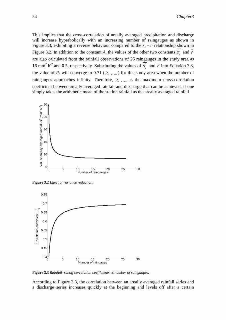
Chapter3 54

This implies that the cross-correlation of areally averaged precipitation and discharge will increase hyperbolically with an increasing number of raingauges as shown in Figure 3.3, exhibiting a reverse behaviour compared to the sx – n relationship shown in Figure 3.2. In addition to the constant A, the values of the other two constants 2

js and r are also calculated from the rainfall observations of 26 raingauges in the study area as 16 mm2 h-2 and 0.5, respectively. Substituting the values of 2

js and r into Equation 3.8, the value of Rk will converge to 0.71 ( ∞→nkR ) for this study area when the number of raingauges approaches infinity. Therefore, ∞→nkR is the maximum cross-correlation coefficient between areally averaged rainfall and discharge that can be achieved, if one simply takes the arithmetic mean of the station rainfall as the areally averaged rainfall.

0 5 10 15 20 25 305

10

15

20

25

30

Number of raingauges

Var

. of a

real

ly a

vera

ged

rain

fall,

s2 (m

m2 h

-2)

Figure 3.2 Effect of variance reduction.

0 5 10 15 20 25 300.4

0.45

0.5

0.55

0.6

0.65

0.7

0.75

Number of raingages

Cor

rela

tion

coef

ficie

nt, R

k

Figure 3.3 Rainfall–runoff correlation coefficients vs number of raingauges.

According to Figure 3.3, the correlation between an areally averaged rainfall series and a discharge series increases quickly at the beginning and levels off after a certain

Appropriate spatial sampling of rainfall for flow simulation 55

threshold. This implies that the similarity between the areally averaged rainfall and discharge series will also increase hyperbolically if one regards Rk as the indicator of the similarity, leading to the expectation that the mathematical mapping between the input and the output can be established more easily. This inference will be tested by a physics-based hydrological model (HBV).

3.4.3 Criterion for appropriateness As shown in Figure 3.3, the increase in the correlation coefficient is no longer significant beyond a certain critical number of raingauges. The improvement in the performance of hydrological modelling is expected to act in a similar way. Therefore, it is concluded that the spatial sampling density of rainfall is already “good enough” for flow simulation, if the number of raingauges is larger than this critical number. This critical number of raingauges is identified as the appropriate number of raingauges, if the first derivative of Rk with respect to n is smaller than or equal to a threshold value, chosen arbitrarily to be 0.01. Therefore, the criterion to find the appropriate number of raingauges is defined as:

( )( ) [ ] 01.0

)1(1

1

2

1d 2/32/12/1

2≤

−+×

−=

rnns

rAn

dR

j

k (3.9)

where A=2 (see page 53). This leads to n ≥ 5 and five is identified as the appropriate number of raingauges for this study area.

3.5 Hydrological modelling It is generally recognized that a simultaneous use of both statistic and physics-based (or deterministic) methods of analysis of hydrological processes is necessary to produce the best scientific and practical information for hydrology (Yevjevich, 1972). Using a statistical method independently of the physics-based one may lead to an analysis of data without a sound theoretical background. Therefore, the conceptual hydrological model HBV is used here to verify the results from the statistical analysis.

The HBV model is a conceptual, semi-distributed hydrological model developed by SMHI (Swedish Meteorological and Hydrological Institute) which is used for continuous computation of discharges at the outlet of a river basin. The model has proven to be a rather robust tool for the assessment of the basin-scale runoff dynamics in various parts of the world (e.g. Bergström, 1995; Zhang and Lindström, 1996; Lindström et al., 1997). Time series data including precipitation, air temperature and estimated potential evapotranspiration are used as inputs to calculate the river discharge (output). Observed discharge series can be used to calibrate the model. In the implementation of the model, the whole considered river basin can be divided into a number of sub-basins. Information about geographical features of the sub-basins is also needed to assemble the model, namely, the area, mean elevation and type of vegetation zones (forest, field, etc.). Each sub-basin can be calibrated separately provided that discharge data at the outlet of the sub-basin are available. The outflow of each sub-basin will be routed to the outlet of the whole basin using the Muskingum method (Linsley et al., 1988) and combined with outflows from other sub-basins, taking into account delaying and damping effects. Each sub-basin model consists of six subroutines: a snow

Chapter3 56

and rainfall routine, a soil routine, a fast flow routine, a slow flow routine, a transformation routine and a routing routine. These sequential subroutines simulate the complete hydrological process from the commencement of precipitation to the formation of discharge at the outlet. Detailed descriptions can be found in SMHI (2003) and Bergström (1995).

For the application of the HBV model to check the results of the statistical analyses, the study area needs to be subdivided into a number of sub-basins. Here, the whole area upstream of Yuxiakou was treated as one sub-basin. Seven years (1989–1995) of hydrological data (precipitation, evaporation and discharge) were used to calibrate the HBV model. Precipitation and evaporation were used as input, and discharge as output. All 26 raingauges available in the area were used to obtain areally averaged rainfall for calibration. The calibrated model was used for validation. During the validation, areally averaged rainfall series were obtained from different numbers (from 1 to 26) of raingauges, and for a specific number of raingauges for different combinations of raingauges, to compare the effect of different spatial sampling strategies on the performance of the calibrated HBV model. Three years (1997–1999) of hydrological data were used for the validation (data of 1996 are missing). The evaporation and discharge data remained the same during the whole validation procedure.

Two statistical criteria are used to judge the performance of the HBV model: the coefficient of efficiency (R2) (Nash & Sutcliffe, 1970) and relative accumulated difference between computed and observed discharge. Their definitions are given in Appendix.

3.6 Results The effects of the number of raingauges on the variance of areally averaged rainfall series and on the cross-correlation between areally averaged rainfall and the discharge are shown in Figures 4 and 5, respectively. To illustrate how the variance decreases as more time series are aggregated, (the variance of n-station averaged time series), is computed for the station data that fall into the area under consideration (Figure 3.1). To obtain the true value of , the variances of every combination of n stations chosen from the N available stations should be computed and their mean, maximum and minimum values taken. For some combinations, such a calculation is not computationally feasible (e.g. there are such combinations when choosing n = 13 from 26 stations available). Therefore, when choosing n ranging from 1 to 7 and 20 to 26, all possible combinations are enumerated, and the combinations which give the maximum and minimum value of variance are selected to draw the boundary lines as shown in Figure 3.4. To present the mean variance, the combination with a variance nearest to the mean variance is taken. For n ranging from 8 to 19, up to 5000 combinations are selected randomly in each case. In order to show that 5000 randomly selected combinations is already enough to produce unbiased means and most of the range (minimum to maximum) of variance and cross-correlation coefficients, the statistics calculated from 10 000 and 15 000 combinations are shown together with the 5000 combinations in Table 3.1. Two numbers of raingauges are chosen to do this analysis. The results revealed that the means and ranges remain essentially the same.

2ns

2ns

710)!13!13/(!26 ≈

Appropriate spatial sampling of rainfall for flow simulation 57

0 5 10 15 20 25 305

10

15

20

25

30

Number of raingauges

Var

ianc

e (m

m2 h

-2)

MeanMaximumMinimum

Figure 3.4 Effect of the number of raingauges on the variance of areally averaged rainfall

0 5 10 15 20 25 300.4

0.45

0.5

0.55

0.6

0.65

0.7

0.75

Number of raingauges

Cro

ss-c

orre

latio

n co

effic

ient

MaximumMeanMinimum

Figure 3.5 Effect of the number of raingauges on the cross-correlation between areally averaged rainfall and discharge.

Table 3.1 The effect of the number of combinations on the statistics of areally averaged rainfall and lagged cross-correlation between areally averaged rainfall and discharge

Variance of areally averaged rainfall (mm2 h-2)

Lagged cross-correlation between areally averaged rainfall and discharge

Number of raingauges

Number of combinations

Min. Mean Max. Min. Mean Max.

5000 6.8 8.5 10.5 0.63 0.66 0.68 10000 6.7 8.5 10.7 0.63 0.66 0.68

12

15000 6.6 8.5 10.7 0.63 0.66 0.68 5000 7.1 8.3 9.7 0.64 0.66 0.68 10000 7.0 8.3 9.9 0.64 0.66 0.68

16

15000 7.1 8.3 10.0 0.64 0.66 0.68

Chapter3 58

As can be seen from Figure 3.4, the variance decreases hyperbolically with an increase in the number of raingauges n. This confirms the expected variance reduction pheno-menon of the areally averaged rainfall series as indicated in Equation 3.1 and Figure 3.2. After a certain threshold, the variance levels off to a final value , which implies that the effect of the variance reduction of areally averaged rainfall series is no longer significant when n is greater than a certain threshold number. As expected, the relationship between the cross-correlation of areally averaged rainfall and discharge and the number of rain stations behaves similarly to the variance reduction effect but in a reverse way (as shown in Figure 3.5): the value of the cross-correlation increases hyperbolically, and levels off after the same threshold, for example, five, as suggested in the previous section. The precise selection of this threshold number of raingauges has to be done together with hydrological modelling results, which are presented below.

2∞s

The HBV modelling results are shown in Figures 6 and 7. The specific combination of rainfall stations was used that gave the maximum, mean and minimum correlation values as shown in Figure 3.5, and the corresponding areally averaged rainfall series was created. These areally averaged rainfall series were used in the simulation with the calibrated HBV model under the expectation that the higher the correlation value, the easier for the model to simulate the rainfall–runoff relationship. Figure 3.6 confirms this expectation because: (a) the combinations which give the maximum correlation values lead to better model performance as indicated by a higher R2 value, compared to the lines which represent the mean and minimum correlation values; and (b) the increase of the R2 value behaves very similarly to the increase in correlation values shown in Figure 3.5; both increase hyperbolically, but level off after a certain threshold. This threshold number of raingauges can be spotted from Figure 3.6, to be five. Beyond this number, a further increase in the number of raingauges will not largely improve the model performance. This confirms the finding in the previous section. Figure 3.7 shows the effect of the number of raingauges on the absolute value of the relative accumulated difference of the discharge. Although the three lines do not decline in parallel as in Figure 3.6, their decrease does exhibit a hyperbolic trend as does the variance reduction behaviour. The fact that the decreasing trend is much more diverse than the lines shown in Figure 3.6 can be explained as follows:

(a) The relative accumulated difference (RD) emphasizes the capability of the model to fulfil the water balance. When the number of raingauges is small and they are selected randomly in the basin, the chance of missing certain rainfall event(s) is quite high, which then leads to big RD values. This is especially the case for small-scale rainfall events.

(b) The specific combination of raingauges used to carry out hydrological simulation is selected by a linear method, whereas the hydrological modelling is a nonlinear process. This discrepancy implies that the minimum and maximum calculations alluded to in Figures 6 and 7 do not fully reflect the minimum and maximum of model performance, and may be part of the reason of the poor behaviour found in Figure 3.7.

Appropriate spatial sampling of rainfall for flow simulation 59

0 5 10 15 20 25 300.2

0.3

0.4

0.5

0.6

0.7

0.8

0.9

1

Number of raingauges

R2

MaximumMeanMinimum

Figure 3.6 Nash-Sutcliffe coefficient vs the number of raingauges.

0 5 10 15 20 25 300

0.02

0.04

0.06

0.08

0.1

0.12

Number of raingauges

Rel

ativ

e A

ccum

ulat

ed D

iffer

ence

MaximumMeanMinimum

Figure 3.7 Absolute value of relative accumulated difference vs the number of raingauges.

Figure 3.8 gives an example of the geographical locations of the combinations of raingauges (from 3 to 7) which give the minimum, mean and maximum cross-correlation between areally averaged rainfall and discharge. Two characteristics of geographical distribution can be detected from the combinations that yield maximum and minimum correlation values: (a) a strong effect of the geographical location: raingauges which yield a maximum correlation value are all located at the centre of the area, whereas the ones that yield the minimum correlation are located in the most remote places; and (b) the addition of new raingauges to the existing raingauges (which give maximum and minimum correlation coefficients) show a successive property. The old ones remain; the new raingauges added are generally based on the existing network for combinations which give the maximum correlation values. So for the combinations that yield minimum and maximum correlation values, the expansion of the network is based on the old raingauges. However, for the combination of raingauges which give

Chapter3 60

the mean correlation value, this is not the case. They are more evenly distributed than the other two cases.

(a) (b) (c)

Figure 3.8 Geographical locations of three combinations of 3–7 raingauges: (a) minimum correlation value, (b) mean correlation value, and (c) maximum correlation value.

3.7 Discussion After superimposing Figure 3.8(c) on the DEM (Digital Elevation Model) map of Figure 3.1, it can be seen that most of the raingauges which yield maximum correlation

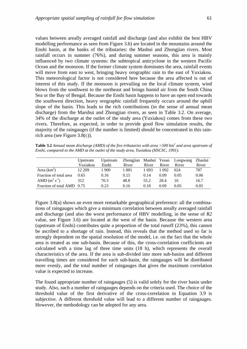
Appropriate spatial sampling of rainfall for flow simulation 61

values between areally averaged rainfall and discharge (and also exhibit the best HBV modelling performance as seen from Figure 3.6) are located in the mountains around the Enshi basin, at the banks of the tributaries: the Mashui and Zhongjian rivers. Most rainfall occurs in summer (76%), and during summer seasons, this area is mainly influenced by two climate systems: the subtropical anticyclone in the western Pacific Ocean and the monsoon. If the former climate system dominates the area, rainfall events will move from east to west, bringing heavy orographic rain to the east of Yuxiakou. This meteorological factor is not considered here because the area affected is out of interest of this study. If the monsoon is prevailing on the local climate system, wind blows from the southwest to the northeast and brings humid air from the South China Sea or the Bay of Bengal. Because the Enshi basin happens to have an open end towards the southwest direction, heavy orographic rainfall frequently occurs around the uphill slope of the basin. This leads to the rich contributions (in the sense of annual mean discharge) from the Marshui and Zhongjian rivers, as seen in Table 3.2. On average, 34% of the discharge at the outlet of the study area (Yuxiakou) comes from these two rivers. Therefore, as expected, in order to provide good flow simulation results, the majority of the raingauges (if the number is limited) should be concentrated in this rain-rich area (see Figure 3.8(c)).

Table 3.2 Annual mean discharge (AMD) of the five tributaries with area >500 km2 and area upstream of Enshi, compared to the AMD at the outlet of the study area, Yuxiakou (HSCSC, 1991).

Upstream Yuxiakou

Upstream Enshi

Zhongjian River

Mashui River

Yesan River

Longwang River

Zhaolai River

Area (km2) 12 209 1 900 1 881 1 693 1 092 624 787 Fraction of total area 0.65 0.16 0.15 0.14 0.09 0.05 0.06 AMD (m3 s-1) 312 70.3 48.8 55.2 28.4 16 16.7 Fraction of total AMD 0.75 0.23 0.16 0.18 0.09 0.05 0.05

Figure 3.8(a) shows an even more remarkable geographical preference: all the combina-tions of raingauges which give a minimum correlation between areally averaged rainfall and discharge (and also the worst performance of HBV modelling, in the sense of R2 value, see Figure 3.6) are located at the west of the basin. Because the western area (upstream of Enshi) contributes quite a proportion of the total runoff (23%), this cannot be ascribed to a shortage of rain. Instead, this reveals that the method used so far is strongly dependent on the spatial resolution of the model, i.e. on the fact that the whole area is treated as one sub-basin. Because of this, the cross-correlation coefficients are calculated with a time lag of three time units (18 h), which represents the overall characteristics of the area. If the area is sub-divided into more sub-basins and different travelling times are considered for each sub-basin, the raingauges will be distributed more evenly, and the total number of raingauges that gives the maximum correlation value is expected to increase.

The found appropriate number of raingauges (5) is valid solely for the river basin under study. Also, such a number of raingauges depends on the criteria used. The choice of the threshold value of the first derivative of the cross-correlation in Equation 3.9 is subjective. A different threshold value will lead to a different number of raingauges. However, the methodology can be adopted for any area.

Chapter3 62

The method used in this study is valid in river basins where a large number of raingauges already exist, and the problem of rational network reduction comes about. If there are very few raingauges, and the river basin manager wants to find out the appropriate number of raingauges, this method will be difficult to implement, because it will be difficult to find out the final value of (Osborn and Hulme, 1997). The methodology used here shows that by looking only at the rainfall–runoff data, one can re-evaluate the efficiency of the network and determine a subset of the most important raingauges, so that the rainfall information provided by these gauges is sufficient for obtaining good flow simulation results.

2∞s

A lumped HBV model was used, which treats the whole study area as one sub-basin, to check the results from the statistical analyses. Therefore, the resulting appropriate number of five raingauges, and their locations will not necessarily stay the same if this HBV model is further developed into a distributed model, i.e. more sub-basins are involved. More rainfall gauges are expected to be necessary in this case. However, the same method can be implemented in each sub-basin to determine the appropriate number of raingauges. The subdivision of the whole basin should be in accordance with the number of discharge gauges in the basin; the outlet of each sub-basin should have at least one flow gauge which observes discharge records. If the parameters in one sub-basin cannot be calibrated according to the observed discharge data, regionalization methods can be used (Seibert, 1999).

The number of raingauges found by this study provides a lower limit of the number of raingauges to be chosen. However, a certain number of additional raingauges should be considered to cope with the possible malfunctioning of the network, and to provide a certain degree of redundant rainfall information for flow simulation. The choice of additional raingauges depends on how the river management authority handles the malfunctioning of the raingauge network.

3.8 Conclusions The effect of an increase in the number of raingauges on the variance reduction of mean areal precipitation and on the increase of the cross-correlation coefficient between mean areal precipitation and discharge was investigated. The aim was to identify the appropriate number of raingauges and their geographical locations for improved flow simulation using a spatially lumped HBV model. The results reveal that the correlation coefficient increases hyperbolically with an increase in the number of raingauges but levels off after a critical number of raingauges, which for this study area turns out to be five. The performance of the lumped HBV model (in terms of coefficient of efficiency, R2) increases in a similar way with the increase in the number of raingauges. Therefore, five was identified to be the sufficient number of raingauges in the study area (for the satisfactory performance of the lumped HBV model). The geographical locations of the raingauge combinations which give the maximum value of correlation coefficient and R2 are strongly correlated with local climatic and geographical conditions. Most of them are located in an area where heavy orographic rainfall is the dominant form of the local precipitation pattern. The combinations of raingauges which gave the worst performance of HBV modelling (and also gave the minimum correlation value) are located in the west of the study area (the farthest from the outlet of the area). This is understandable, because the farthest raingauges will have the least influence on the

Appropriate spatial sampling of rainfall for flow simulation 63

runoff at the outlet if one treats the whole area as only one sub-basin in the HBV model. However, if the study area is divided into multiple sub-basins, the raingauges which give the worst performance of the HBV model may be located elsewhere. One can conclude that the methodology introduced herein is dependent on the spatial resolution of the model.

Chapter3 64

Chapter 4

Appropriate application of artificial neural networks for flow forecasting

Abstract In this chapter the appropriate complexity and appropriate training of an Artificial Neural Network (ANN) are determined. For an ANN, ‘complexity’ refers to the network structure and thus to the number of neurons in the network. The ANN is used for one-day ahead forecasting of the discharge in the river Meuse (western Europe) at Borgharen (in the south of the Netherlands), based on the recorded precipitation upstream of Borgharen. The forecasting performance is measured with the Nash-Sutcliffe coefficient R2 and the Relative Mean Absolute Error RMAE, the applied training algorithm is the Levenberg-Marquardt (LM) algorithm and the applied performance function is the Mean Square Error (MSE). All networks are trained multiple times, so that not only the mean of the R2 and the RMAE values are calculated, but also the standard deviations to evaluate their uncertainties.

First, the numbers of input and hidden neurons are varied to determine the effect of network complexity on the forecasting performance. Secondly, the influence of weight decay on the forecasting performance is determined for different network complexities. Weight decay is a method used to train an ANN with a modified performance function, which normally is MSE. For weight decay, a penalty term is added to the performance function to prevent the values of the weights and biases becoming too large during the training to enable a smoother network response. Different degrees of weight decay influence are introduced by varying the value of the “decay coefficient” from 0.1 to 1, with higher values corresponding to a smaller influence of weight decay. Network complexity is now expressed in terms of the total number of neurons in the network. Thirdly, the effect of the number of training epochs (or iterations) on the forecasting performance is determined, again for different network complexities in terms of total number of neurons in the network.

The network structure (or complexity) has the largest influence on the flow forecasting performance. The influence of the number of training epochs is somewhat smaller, and weight decay has the smallest influence on the flow forecasting performance. An 8-4-1 network (8 neurons in the input layer, 4 in the hidden layer and 1 in the output layer) trained for 11 epochs with no weight decaying being applied was identified as an appropriate network. Networks simpler than an 8-4-1 network should be trained more than 13 epochs. For networks more complex than an 8-4-1 network, the appropriate training epochs range between 8 and 11. For a simple network, weight decay is not a useful method to improve the network’s generalization ability. For a complex network, weight decay can help to prevent overfitting, by compensating for the negative influence of a greater network complexity on network performance.

Chapter4 66

4.1 Introduction

4.1.1 The principle of artificial neural networks An Artificial Neural Network (ANN) is 'a massively parallel distributed processor made up of simple processing units, which has a natural propensity for storing experimental knowledge and making it available for use' (Haykin, 1999).

ANNs consist of a number of hierarchical layers. Each layer consists of a number of simple artificial processing units, artificial neurons; in this study, the artificial neurons will simply be termed neurons. They are placed parallel to each other, and are connected by links in which knowledge is stored. Obtaining and updating knowledge are accomplished by a process called training (or learning). Training can strengthen the links among neurons, similar to how human brains strengthen their memories: the more times the learning process is repeated, the stronger linkages will be established among the neurons that are responsible for storing this knowledge. Strong links will lead to a quick recall of the knowledge when information similar to what has been used in training is fed into the network as input.

4.1.2 The structure of artificial neural networks Figure 4.1 shows a simple ANN. It consists of an input layer, a hidden layer and an output layer. In this example, these layers have one, two and one neurons, respectively. An ANN with such a structure is called a 1-2-1 ANN. Neurons in different layers are 'one-way connected' in this example, which for this type of ANN means that information flows only from the input to output layer, not the other way around. The input neuron receives input data or information (shown in Figure 4.1 as p) from outside, then passes it on to all the neurons in the hidden layer multiplied by w1 and w2. Next, the hidden neurons receive and transform (explained in next paragraph) the received information to the output neuron. The output neuron also transforms the received information. Its output a will be the network’s output. Because the input neuron does not change the input information (as a normal biological neuron would do) and simply re-distributes the received information, some researchers call it 'input node' (Haykin, 1999). In this research, for the sake of uniformity (and simplicity), it is still called 'input neuron'.

Figure 4.1 An ANN with one input neuron, two hidden neurons and one output neuron.

The information transformation process in the hidden and output neurons is performed in three steps:

Appropriate application of artificial neural networks for flow forecasting 67

(1) Each piece of information is multiplied by a 'weight' (like the parameter w4 shown in Figure 4.1, which is the weight connecting hidden neuron 2 with output neuron 1), and then summed.

(2) An externally applied 'bias' (denoted as, e.g. b3, in Figure 4.1) is added to the weighted summation. Biases have the effect of increasing or lowering the output of the neurons, depending on whether the bias is positive or negative, respectively.

(3) Once the inputs are weighted, summed, and biased, a so-called 'transfer function' is applied to transform the information. The transfer function can be either linear or non-linear.

Normally, the transfer functions for neurons in the same layer are the same, but they can also be different. If the transfer functions in the hidden and output layers are denoted as f1 and f2 respectively, the output a of the network shown in Figure 4.1 can be written as:

[ ] [ ]{ 3221411132 bbpwfwbpwfwfa }++++= (4.1)

4.1.3 Training artificial neural networks Once the ANN has been constructed, the parameters (the weights and biases) inside the network need to be adjusted so that the calculated output (a) can match the real output (or response) of the modelled physical system, with the same input (p) presented to both the network and the physical system. The ANN’s approach to adjust the parameters is:

(1) Give its parameters random values in a process called initialization.

(2) Transfer the inputs from the input to output neurons and calculate the network outputs.

(3) Calculate the error between the network output and observed output (of the real physical system) with a so-called performance function, which normally is the Mean Square Error (MSE) between the network and observed output.

(4) Adjust the parameters to minimize the error - MSE. First, gradients are calculated, which are the derivatives of MSE with respect to the network weights and biases. Then, the weights and biases are adjusted in a direction negative to the gradients so as to enable a decrease in MSE.

(5) The parameters will be adjusted again and again, until the calculated network output matches the real observed output according to a certain criterion. This process is called training. The data used to train an ANN are called training data sets. A number of algorithms have been developed to train ANNs efficiently.

(6) After training, use a different data set to measure the network’s capability to estimate the output in case that different input is fed into the network. This process is called testing, and the data sets used are called testing data sets.

Chapter4 68

The advantage of such an approach is that an ANN with a sufficient number of hidden neurons (which implies that the structure of the ANN is complex enough) is able to approximate any continuous function to any degree of accuracy, if enough training is performed (Coulibaly et al., 2000). The risk of this approach is that the network may be too complex and be trained too much, that it overfits the input-output relation. This is discussed in the next section.

There are two modes of training for updating the parameters during the training process. One is called incremental training mode. In this style of training, the weights and biases of the network are updated each time after an input is applied to the network. The second one is batch mode. In this case, the weights and biases are only updated after the entire training set (inputs and observed outputs) has been applied to the network. The gradients calculated at each training example are averaged to produce a more accurate estimation of the gradient. The Levenberg-Marquardt algorithm (Hagan et al., 1996) used in this study uses a batch mode to update the parameters of the network. One round of training – which includes (1) presenting the whole training set to a network, (2) calculating the gradient, and (3) updating the weights and biases – is called one training epoch. The number of training epochs should be appropriately selected to prevent overfitting.

4.1.4 Overfitting and generalization If an ANN is very complex and trained too much, the error (difference between the network output and the observed output) may be driven to a too small value. Then, in the testing phase, when new data are presented to the network, the error may be much larger than the error in the training process. This implies that the network fits the training data so closely, that it has not learned to generalize to new situations. This phenomenon is called overfitting. The studied data set may also be underfitted, if the ANN is not sufficiently complex and has not been trained enough to detect the signals within the data set fully.

Figure 4.2 shows the response of a 1-20-1 ANN to a noisy sine function as input. The ANN has been trained 1000 times to approximate the underlying sine function. It is seen from the figure that the ANN is trying to catch all the details of the input data, but misses the more important, general information. In other words, it shows a lack of generalization. For comparison, Figure 4.2 also displays the output of a 1-5-1 network trained 10 times with the same input data set. It matches the underlying sine function much better than the output from the overfitted network.

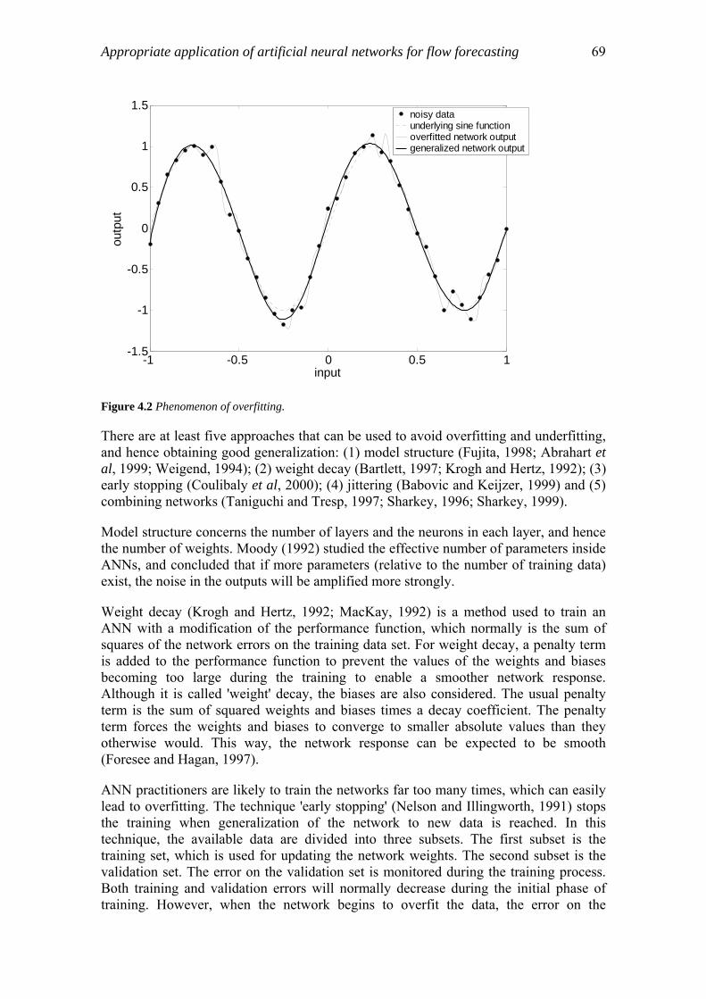
Appropriate application of artificial neural networks for flow forecasting 69

-1 -0.5 0 0.5 1-1.5

-1

-0.5

0

0.5

1

1.5

input

outp

utnoisy dataunderlying sine functionoverfitted network outputgeneralized network output

Figure 4.2 Phenomenon of overfitting.

There are at least five approaches that can be used to avoid overfitting and underfitting, and hence obtaining good generalization: (1) model structure (Fujita, 1998; Abrahart et al, 1999; Weigend, 1994); (2) weight decay (Bartlett, 1997; Krogh and Hertz, 1992); (3) early stopping (Coulibaly et al, 2000); (4) jittering (Babovic and Keijzer, 1999) and (5) combining networks (Taniguchi and Tresp, 1997; Sharkey, 1996; Sharkey, 1999).

Model structure concerns the number of layers and the neurons in each layer, and hence the number of weights. Moody (1992) studied the effective number of parameters inside ANNs, and concluded that if more parameters (relative to the number of training data) exist, the noise in the outputs will be amplified more strongly.

Weight decay (Krogh and Hertz, 1992; MacKay, 1992) is a method used to train an ANN with a modification of the performance function, which normally is the sum of squares of the network errors on the training data set. For weight decay, a penalty term is added to the performance function to prevent the values of the weights and biases becoming too large during the training to enable a smoother network response. Although it is called 'weight' decay, the biases are also considered. The usual penalty term is the sum of squared weights and biases times a decay coefficient. The penalty term forces the weights and biases to converge to smaller absolute values than they otherwise would. This way, the network response can be expected to be smooth (Foresee and Hagan, 1997).

ANN practitioners are likely to train the networks far too many times, which can easily lead to overfitting. The technique 'early stopping' (Nelson and Illingworth, 1991) stops the training when generalization of the network to new data is reached. In this technique, the available data are divided into three subsets. The first subset is the training set, which is used for updating the network weights. The second subset is the validation set. The error on the validation set is monitored during the training process. Both training and validation errors will normally decrease during the initial phase of training. However, when the network begins to overfit the data, the error on the

Chapter4 70

validation set will typically begin to rise. When the validation error starts to increase, the training is stopped. The so-derived weights and biases will be used for testing. The testing set error is not used during the training, but used to compare different models.

There are other techniques to help and improve the generalization of ANNs, like jittering (training network with noise) (Holmströn and Koistinen, 1992; Koistinen and Holmströn, 1992; An, 1996), Bayesian learning (an efficient way to estimate the value of the constant to adjust the penalty strength when performance function modification is used to prevent overfitting) (Foresee and Hagan, 1997), and combining networks (Sharkey, 1996; Sharkey, 1999). They will not be considered in detail in this study. Only weight decay and early stopping are taken as examples to study the effects of these two measures on improving the network performance.

4.1.5 Appropriate modelling in the context of applying ANNs in flow forecasting

In the above-mentioned three methods, model structure is important, in the sense that it has to be appropriate for the modelled system, for the available data, and for the objective of modelling. Weight decay and early stopping are related to the training of the model (that is, the process of adjusting model parameters). Note that in case of physics-based models, this is called calibration.

Both the structure and the training of ANN models should be appropriate: the structure has to be appropriately complex and the strength of the training of the network has to be appropriate. Losing control on both issues will lead to overfitting or underfitting to the data.

For the research carried out in applying ANNs in flow forecasting, the following two research gaps are identified:

(1) So far, most research into applying ANNs in flow forecasting has been performed in a single-training way (Govindaraju and Ramachandra Rao, 2000; Dong and Vreugdenhil, 2002). That means the ANN is trained once, and one flow forecasting performance value is obtained. The disadvantage of this method is that each time the network is re-trained, the forecasting performance will be different (no matter how slightly). This is because before each training, all parameters are re-initialized randomly. For different trainings, the final values of parameters are different each time. So what is the uncertainty of the obtained forecasting performance?

(2) The methods used to prevent overfitting are applied individually. However, they are actually correlated, so what is their collective effect on flow forecasting performance? More specifically, how do the appropriate model structure and training process influence model performance?

4.1.6 Research questions The following research questions are addressed in this chapter:

(1) Because of the stochastic nature of the initialization and training process, how should the forecasting performance be evaluated statistically?

Appropriate application of artificial neural networks for flow forecasting 71

(2) What is the appropriate structure of an ANN-based model for flow forecasting?

(3) As a remedy to overfitting, how can weight decay improve the generalization capability of ANNs for flow forecasting?

(4) For a certain training algorithm, how many training epochs are appropriate, beyond which further training is deleterious?

(5) Which one is more influential on improving flow forecasting performance: an appropriate model structure, applying weight decay or early stopping in training?

4.1.7 Research approach and outline of this chapter The remainder of this chapter is arranged according to the logic of applying an ANN model. In Section 4.2, the physical conditions of the studied area are introduced; followed by a description of the data that are selected for training, validation and testing purposes and a description of how this selection is made. In Section 4.3, a prototype ANN model is constructed, and applied for flow forecasting. In Section 4.4, the appropriate model complexity is studied with regard to its influence on the flow forecasting performance. After determining the appropriate model structure, the appropriate training method is investigated in Section 4.5 and 4.6. Here, two methods to prevent overfitting are considered: weight decay (in Section 4.5) and training the network with an appropriate number of epochs (in section 4.6). For all the methods used, the networks are trained multiple times, so that not only the mean values but also the standard deviations of the network performances are evaluated. In all of these sections, the methodologies will be presented first, followed by the results. The discussion of these results follows in Section 4.7. Finally, conclusions are drawn in Section 4.8.

4.2 Case study area and data The Meuse River in Western Europe is taken as case study in this chapter, because of the following three reasons:

(1) The current PhD-project is a joint Chinese-Dutch research project. In Chapters 2 and 3 a Chinese river has been used as case study. In order to promote the knowledge exchange between China and the Netherlands, it is preferred to also use a Dutch river as case study in this project.

(2) by the time this study was being carried out, hydrological data from the Meuse River were the most easily accessible ones;

(3) The main objective of this study is to develop a methodology to apply flow forecasting models (in this case an ANN) appropriately. This is not dependent on the specific river being studied. In fact, using a different river as case study shows the general applicability of the methodology.

The Meuse River originates in France, flows to the north, through Belgium and joins the North Sea in The Netherlands. The river is 878 km long and has a catchment of about

Chapter4 72

33,000 km2 (Figure 4.3). For this research, only the part of the Meuse upstream of Borgharen (in the south-east of The Netherlands, near Maastricht) is taken into account.

Figure 4.3 The Meuse River basin (Berger, 1992).

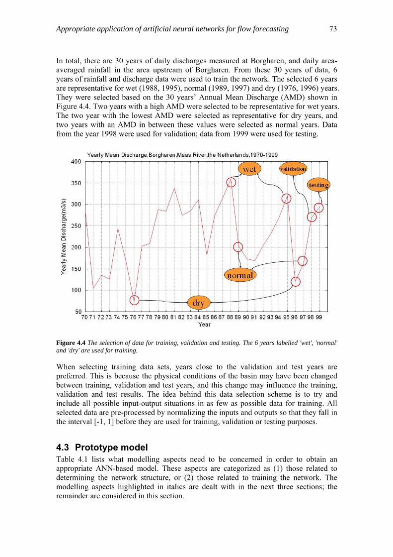
Appropriate application of artificial neural networks for flow forecasting 73

In total, there are 30 years of daily discharges measured at Borgharen, and daily area-averaged rainfall in the area upstream of Borgharen. From these 30 years of data, 6 years of rainfall and discharge data were used to train the network. The selected 6 years are representative for wet (1988, 1995), normal (1989, 1997) and dry (1976, 1996) years. They were selected based on the 30 years’ Annual Mean Discharge (AMD) shown in Figure 4.4. Two years with a high AMD were selected to be representative for wet years. The two year with the lowest AMD were selected as representative for dry years, and two years with an AMD in between these values were selected as normal years. Data from the year 1998 were used for validation; data from 1999 were used for testing.

Figure 4.4 The selection of data for training, validation and testing. The 6 years labelled 'wet', 'normal' and 'dry' are used for training.

When selecting training data sets, years close to the validation and test years are preferred. This is because the physical conditions of the basin may have been changed between training, validation and test years, and this change may influence the training, validation and test results. The idea behind this data selection scheme is to try and include all possible input-output situations in as few as possible data for training. All selected data are pre-processed by normalizing the inputs and outputs so that they fall in the interval [-1, 1] before they are used for training, validation or testing purposes.

4.3 Prototype model Table 4.1 lists what modelling aspects need to be concerned in order to obtain an appropriate ANN-based model. These aspects are categorized as (1) those related to determining the network structure, or (2) those related to training the network. The modelling aspects highlighted in italics are dealt with in the next three sections; the remainder are considered in this section.

Chapter4 74

Table 4.1 Aspects that need to be considered to determine the appropriate ANN-based model.

network architecture

number of layers

number of neurons in each layer *

type of input variables

type of output variables

Mod

el s

truct

ure

type of transfer functions

training algorithm

appropriate performance function-weight decay *

appropriate training epochs-early stopping *

appropriate amount of training data sets

Tra

inin

g pr

oces

s

the validation and testing data sets * Dealt with in this research; the rest is addressed in this section.

4.3.1 Model architecture and number of layers There are three fundamentally different classes of ANN architecture: single-layer feed-forward networks, multi-layer feed-forward (MLFF), and recurrent networks (Haykin, 1999). The network architecture of the ANNs used in this study is MLFF. MLFF was chosen because theoretically, it is capable of approximating complicated nonlinear (differential and bounded) functions to arbitrary accuracy (Funahashi, 1989; Hornik et al., 1989; Hornik, 1991). In practice, a three-layer MLFF network that contains one input layer (with no transfer function), one hidden layer with nonlinear transfer functions, and one output layer with linear transfer functions is usually sophisticated enough to approximate any nonlinear function as long as sufficient neurons in the hidden layer are available (Haykin, 1999). The input layer does not change the input information, but receives it and passes it to all hidden neurons. Therefore, the basic configuration of the model used is a three-layer MLFF network.

4.3.2 Input, output variables and transfer functions In this research, the modelling goal of ANNs is to use daily rainfall and discharge data to forecast discharges with a lead time of one day. So the type of output variable is discharge, and correspondingly, there is only one neuron in the output layer. There are two types of input variables: rainfall and discharge. The number of neurons in the input layer depends on how many days of data prior to the forecasting will be used. How many days of data prior to the forecasting should be used is, in turn, related to the hydrological response time of the river basin. For example, if a basin is a 'slow-response' basin, then more days of data prior to the forecasting are needed because the rainfall and discharge from a long time ago can still influence the discharge at the time of the forecast.

Figure 4.5(a) shows the lagged auto-correlation coefficient of the discharge at Borgharen. It reveals that the correlations between the lagged discharges are strong (e.g., the correlation coefficient between discharges with a time lag of 30 days is still as

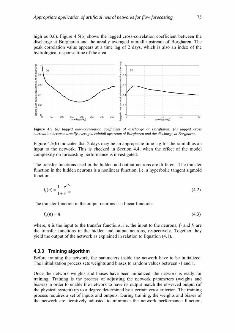
Appropriate application of artificial neural networks for flow forecasting 75

high as 0.6). Figure 4.5(b) shows the lagged cross-correlation coefficient between the discharge at Borgharen and the areally averaged rainfall upstream of Borgharen. The peak correlation value appears at a time lag of 2 days, which is also an index of the hydrological response time of the area.

0 50 100 150 200 250 300 3500

0.2

0.4

0.6

0.8

1

(a)

time lag (day)

lagg

ed a

uto-

corre

latio

n co

effic

ient

of d

isch

arge

0 5 10 15 200

0.2

0.4

0.6

0.8

1

(b)

time lag (day)lagg

ed c

ross

cor

rela

tion

betw

een

rain

fall

and

disc

harg

e

Figure 4.5 (a) lagged auto-correlation coefficient of discharge at Borgharen; (b) lagged cross correlation between areally averaged rainfall upstream of Borgharen and the discharge at Borgharen.

Figure 4.5(b) indicates that 2 days may be an appropriate time lag for the rainfall as an input to the network. This is checked in Section 4.4, when the effect of the model complexity on forecasting performance is investigated.

The transfer functions used in the hidden and output neurons are different. The transfer function in the hidden neurons is a nonlinear function, i.e. a hyperbolic tangent sigmoid function:

n

n

eenf 2

2

1 11)( −

−

+−

= (4.2)

The transfer function in the output neurons is a linear function:

nnf =)(2 (4.3)

where, n is the input to the transfer functions, i.e. the input to the neurons; f1 and f2 are the transfer functions in the hidden and output neurons, respectively. Together they yield the output of the network as explained in relation to Equation (4.1).

4.3.3 Training algorithm Before training the network, the parameters inside the network have to be initialized. The initialization process sets weights and biases to random values between -1 and 1.

Once the network weights and biases have been initialized, the network is ready for training. Training is the process of adjusting the network parameters (weights and biases) in order to enable the network to have its output match the observed output (of the physical system) up to a degree determined by a certain error criterion. The training process requires a set of inputs and outputs. During training, the weights and biases of the network are iteratively adjusted to minimize the network performance function,

Chapter4 76

which is normally the Mean Square Error (MSE). The training algorithm has to determine how to use the gradient of the performance function to adjust the weights and biases. The best-known method is the back-propagation (BP) algorithm.

The simplest implementation of back-propagation training updates the network weights and biases in the direction in which the performance function decreases most rapidly (that is, at the greatest negative gradient). One iteration of this algorithm can be written as:

kkkk gxx α−=+1 (4.4)

where is a vector of current weights and biases, is the current gradient, and kx kg kα is the learning rate.

The disadvantage of the original version of the BP algorithm is that its convergence process is very slow. In order to increase the efficiency of the training process, many new training algorithms have been developed. The one used in this research is the so-called Levenberg-Marquardt (LM) algorithm (Hagan et al., 1996). The LM algorithm updates the value of weights and biases in the following way:

[ ] eJIJJxx TTkk

11

−

+ +−= µ (4.5)

where J is the Jacobian matrix that contains the first derivatives of the network errors with respect to the weights and biases; e is a vector of network errors; I is the identity matrix. µ is a changeable coefficient called the Marquardt parameter. It is introduced to adjust the convergence rate. The algorithm begins with µ set to a small value (e.g., 0.01). If one training iteration does not yield a smaller value of the performance function (MSE), this means that the training is not in the right direction. Then the next training iteration will be performed with a larger value of µ to guarantee the decrease of the performance function in the steepest direction. If a training iteration does produce a smaller value of the performance function, the value of µ will be decreased so that the next searching step will be smaller to enable a robust searching process. In this manner, the algorithm provides a good compromise between the training speed and the guaranteed convergence of the steepest descent.

The selection of training, validation and testing data sets has been described in Section 4.2.

4.4 Appropriate number of neurons in input and hidden layers In this research, an MLFF with 3 layers was set up for one-day-ahead flow forecasting. This one-day-ahead flow forecasting was accomplished under the assumption that the flow observed at time t – – can be forecasted by using observed rainfall )(tQ )( itP − and discharge )( itQ − data from preceding days, according to the general relationship:

( ) )()(...,),1(),(...,),1()( teitPtPitQtQftQ pq +−−−−= (4.6)

Appropriate application of artificial neural networks for flow forecasting 77

where f is the assumed input-output function (or relationship), iq and ip are the number of past inputs and outputs, respectively, contributing to the present output, and e(t) is the unknown forecasting error.

The aim of this section is to determine the appropriate combinations of number of neurons in the input and the hidden layers.

Two types of input, rainfall and discharge, are considered here, therefore, the minimum number of input neurons is 2. The number of data from the past used as input determines the total number of input neurons. For example, if 5 days of rainfall and discharge data are used as input, there will be 2 × 5 = 10 input neurons. In this research, the number of input neurons is varied from 2 to 20. The number of hidden neurons ranges from 1 to 10. More tests showed that further increase of the input (and hidden) neurons was not necessary, because it would lead to a decrease in the forecasting performance (measured with the Nash-Sutcliffe coefficient (R2) and the Relative Mean Absolute Error (RMAE)), which implied that the network was too complex to generalize to the testing data set. The definitions of R2 and RMAE are given in Appendix.

For each number of input neurons and number of hidden neurons, the network is trained and tested 40 times, so that not only the mean, but also the variations of the forecasting performance indices (R2 and RMAE) are obtained. Further research might be necessary to determine how many times of this training and testing process are necessary to reach a certain confidence level of the results.

Each time, the training stops when the performance function (MSE, the Mean Square Error between network output and observed output) reaches 0.001. The stop training criterion (MSE=0.001) was obtained by trial and error, when the trained network generalizes well to the testing data set. Then, the mean values of the 40 forecasting performance indices (R2 and RMAE) are calculated to determine the effect of the network complexity (the number of input and hidden neurons) on the forecasting performance. Also, the standard deviations of the 40 R2 and RMAE values are calculated to measure the uncertainty behind this relationship. Figure 4.6 gives an overview of these results.

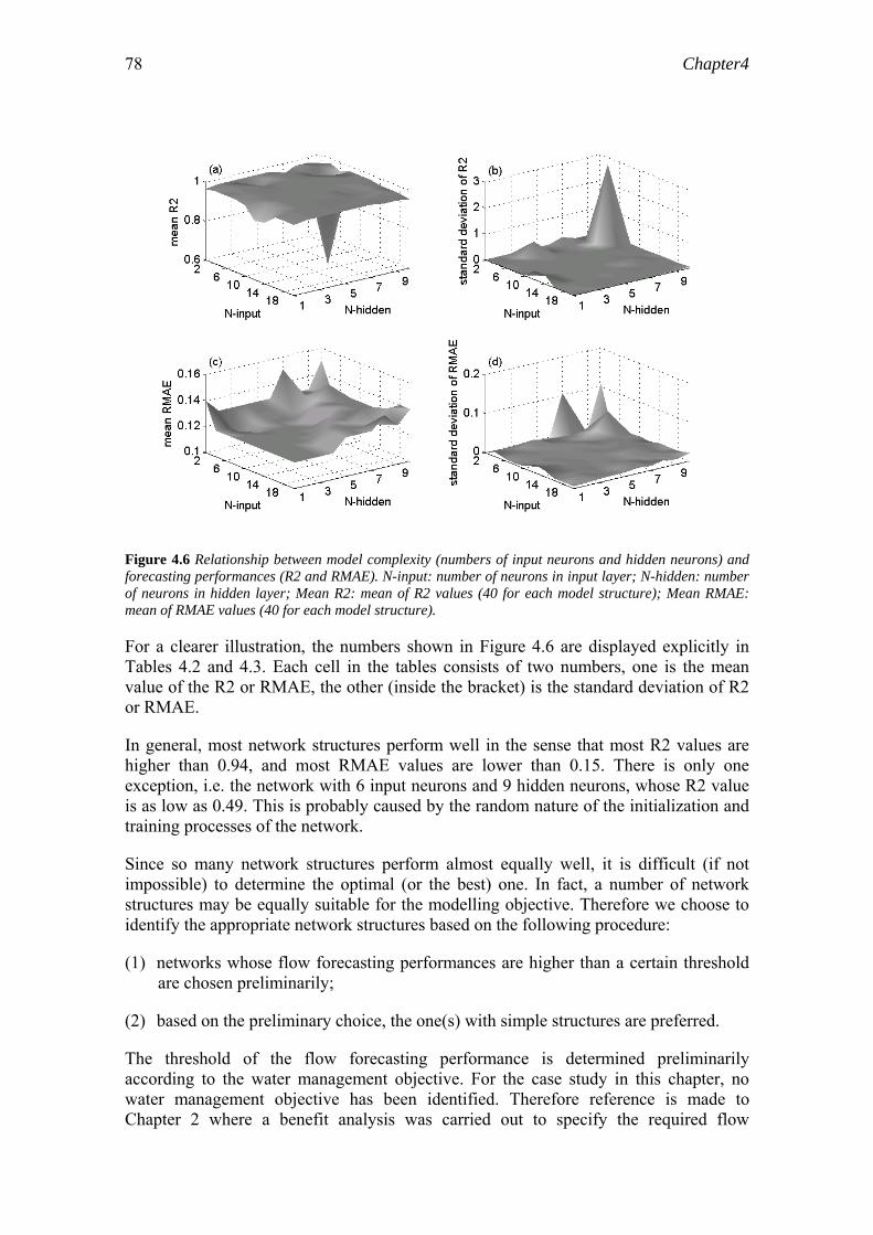
Chapter4 78

Figure 4.6 Relationship between model complexity (numbers of input neurons and hidden neurons) and forecasting performances (R2 and RMAE). N-input: number of neurons in input layer; N-hidden: number of neurons in hidden layer; Mean R2: mean of R2 values (40 for each model structure); Mean RMAE: mean of RMAE values (40 for each model structure).

For a clearer illustration, the numbers shown in Figure 4.6 are displayed explicitly in Tables 4.2 and 4.3. Each cell in the tables consists of two numbers, one is the mean value of the R2 or RMAE, the other (inside the bracket) is the standard deviation of R2 or RMAE.

In general, most network structures perform well in the sense that most R2 values are higher than 0.94, and most RMAE values are lower than 0.15. There is only one exception, i.e. the network with 6 input neurons and 9 hidden neurons, whose R2 value is as low as 0.49. This is probably caused by the random nature of the initialization and training processes of the network.

Since so many network structures perform almost equally well, it is difficult (if not impossible) to determine the optimal (or the best) one. In fact, a number of network structures may be equally suitable for the modelling objective. Therefore we choose to identify the appropriate network structures based on the following procedure:

(1) networks whose flow forecasting performances are higher than a certain threshold are chosen preliminarily;

(2) based on the preliminary choice, the one(s) with simple structures are preferred.

The threshold of the flow forecasting performance is determined preliminarily according to the water management objective. For the case study in this chapter, no water management objective has been identified. Therefore reference is made to Chapter 2 where a benefit analysis was carried out to specify the required flow

Appropriate application of artificial neural networks for flow forecasting 79

forecasting performance in terms of required R2 and RMAE values. For the case studied in chapter 2, if an 80% benchmark benefit (theoretical maximum benefit) is desired, then a 4-day ahead flow forecasting with a performance of 0.90 (in terms of R2 values; or 0.25 in terms of RMAE values) is necessary to meet the desired benefits. The same methodology could be applied to derive the required values of R2 and RMAE for a one-day ahead flow forecasting for the Meuse River. For now, we just assume that an R2 value of 0.98 is the determined threshold value.

There are 5 network structures whose R2 values are higher than 0.98. They are networks with 4, 6 and 8 input neurons combined with 2 or 3 hidden neurons. They are highlighted in Table 4.2 with a black background. The second step in the procedure to determine the appropriate network(s) can be considered as the application of the “principle of parsimony”. The “principle of parsimony”, which is also called “Ockham's Razor”, is a principle attributed to the 14th century English logician and Franciscan friar, William of Ockham that forms the basis of methodological reductionism. William wrote, in Latin, “Pluralitas non est ponenda sine necessitate”, which translates literally into English as “Plurality should not be posited without necessity” (Thorburn, 1915; Thorburn, 1918). To be applied in the context of appropriate modelling in this study, this principle can be translated as “the simplest model (or network) is preferred, as long as the objective is met”. Therefore, the network with a structure of 4-2-1 is selected as the appropriate network. Note that the appropriate training method has not yet been considered in determining the appropriate network.

Table 4.2 Values of mean R2 and standard deviation of R2 (in the brackets) for different values of N-input (number of input neurons) and N-hidden (number of hidden neurons). The highlighted mean R2 values are values higher than or equal to 0.98.Some standard deviations of mean R2 are rounded to be 0.00, for the number of significant digits is taken to be 2.

→ Number of hidden neurons ↓ 1 2 3 4 5 6 7 8 9 10

2 0.96 (0.00)

0.97 (0.00)

0.97 (0.00)

0.97 (0.00)

0.97 (0.00)

0.97 (0.00)

0.94 (0.17)

0.97 (0.00)

0.97 (0.00)

0.94 (0.17)

4 0.97 (0.02)

0.98 (0.01)

0.98 (0.01)

0.90 (0.49)

0.97 (0.01)

0.97 (0.03)

0.97 (0.01)

0.96 (0.03)

0.97 (0.01)

0.97 (0.01)

6 0.97 (0.00)

0.97 (0.02)

0.98 (0.00)

0.97 (0.01)

0.97 (0.04)

0.97 (0.01)

0.97 (0.01)

0.96 (0.09)

0.49 (3.01)

0.95 (0.10)

8 0.97 (0.00)

0.98 (0.00)

0.98 (0.00)

0.97 (0.01)

0.97 (0.01)

0.97 (0.02)

0.97 (0.01)

0.97 (0.01)

0.97 (0.01)

0.97 (0.02)

10 0.96 (0.03)

0.97 (0.01)

0.97 (0.02)

0.97 (0.00)

0.97 (0.01)

0.97 (0.01)

0.97 (0.01)

0.97 (0.01)

0.97 (0.01)

0.97 (0.01)

12 0.90 (0.34)

0.97 (0.00)

0.97 (0.01)

0.97 (0.01)

0.97 (0.01)

0.97 (0.01)

0.97 (0.01)

0.97 (0.01)

0.97 (0.01)

0.97 (0.01)

14 0.91 (0.35)

0.97 (0.01)

0.97 (0.01)

0.97 (0.01)

0.97 (0.01)

0.97 (0.01)

0.97 (0.01)

0.94 (0.14)

0.96 (0.03)

0.96 (0.03)

16 0.96 (0.01)

0.97 (0.01)

0.97 (0.01)

0.97 (0.01)

0.97 (0.01)

0.96 (0.05)

0.96 (0.02)

0.95 (0.03)

0.97 (0.01)

0.96 (0.02)

18 0.96 (0.02)

0.97 (0.03)

0.97 (0.04)

0.97 (0.01)

0.97 (0.01)

0.96 (0.03)

0.97 (0.01)

0.96 (0.02)

0.96 (0.02)

0.96 (0.02)

Num

ber o

f inp

ut n

euro

ns

20 0.96 (0.02)

0.97 (0.01)

0.97 (0.01)

0.97 (0.01)

0.97 (0.01)

0.97 (0.01)

0.97 (0.01)

0.96 (0.02)

0.96 (0.01)

0.95 (0.06)

Chapter4 80

Table 4.3 Values of mean RMAE and standard deviation of RMAE (in the brackets) for different values of N-input (number of input neurons) and N-hidden (number of hidden neurons). The highlighted RMAE values are values higher than or equal to 0.11. Some standard deviations of mean RMAE are rounded to be 0.00, for the number of significant digits is taken to be 2.

→ Number of hidden neurons ↓ 1 2 3 4 5 6 7 8 9 10

2 0.14 (0.00)

0.13 (0.00)

0.13 (0.00)

0.13 (0.00)

0.13 (0.00)

0.13 (0.00)

0.15 (0.11)

0.13 (0.00)

0.13 (0.00)

0.15 (0.11)

4 0.12 (0.01)

0.12 (0.01)

0.11 (0.01)

0.12 (0.02)

0.12 (0.01)

0.12 (0.01)

0.12 (0.01)

0.13 (0.01)

0.13 (0.01)

0.13 (0.01)

6 0.12 (0.01)

0.12 (0.01)

0.11 (0.01)

0.12 (0.01)

0.12 (0.01)

0.12 (0.01)

0.12 (0.01)

0.13 (0.02)

0.14 (0.06)

0.13 (0.02)

8 0.12 (0.00)

0.12 (0.00)

0.12 (0.01)

0.12 (0.01)

0.12 (0.01)

0.12 (0.01)

0.13 (0.01)

0.13 (0.01)

0.13 (0.01)

0.13 (0.01)

10 0.12 (0.01)

0.12 (0.01)

0.12 (0.01)

0.12 (0.01)

0.12 (0.01)

0.12 (0.01)

0.12 (0.01)

0.13 (0.01)

0.13 (0.01)

0.13 (0.01)

12 0.12 (0.02)

0.12 (0.01)

0.12 (0.01)

0.12 (0.01)

0.12 (0.01)

0.12 (0.01)

0.13 (0.01)

0.13 (0.01)

0.13 (0.01)

0.13 (0.01)

14 0.12 (0.02)

0.12 (0.01)

0.12 (0.01)

0.12 (0.01)

0.12 (0.01)

0.13 (0.01)

0.13 (0.01)

0.13 (0.02)

0.13 (0.01)

0.13 (0.01)

16 0.12 (0.01)

0.12 (0.01)

0.12 (0.01)

0.12 (0.01)

0.13 (0.01)

0.13 (0.01)

0.13 (0.01)

0.14 (0.02)

0.13 (0.01)

0.13 (0.01)

18 0.12 (0.01)

0.12 (0.01)

0.12 (0.01)

0.12 (0.01)

0.13 (0.01)

0.13 (0.02)

0.13 (0.01)

0.13 (0.01)

0.14 (0.02)

0.14 (0.02)

Num

ber o

f inp

ut n

euro

ns

20 0.12 (0.01)

0.12 (0.01)

0.12 (0.01)

0.12 (0.01)

0.13 (0.01)

0.13 (0.01)

0.13 (0.01)

0.14 (0.02)

0.13 (0.01)

0.14 (0.02)

Another important aspect in ANN-based modelling, the training of the ANNs, has not been considered so far. As being stated in Sub-section 4.1.4, a network being trained too much can also lead to overfitting to the training data set, therefore deteriorate the network performance on testing data set. The following two sections, Section 4.5 and 4.6, will determine what is the appropriate training process and its relationship with the network structure.

4.5 Weight decay Weight decay is a way of improving the network’s generalization ability by modifying its performance function (MSE), which was proposed by MacKay (1992). The idea is to try and keep the absolute values of weights (and biases, although it is called 'weight decay') in a network small. In that case, the network response should be smooth. Thus, even if the network is slightly oversized, it should be able to represent the underlying true function, rather than capture the noise. The typical performance function that is used for training MLFF is the Mean Square Error (MSE): the average squared error between the network outputs and the observed outputs : '

tQ tQ

( ) NQQEN

tttD /

1

2' ⎟⎠

⎞⎜⎝

⎛−= ∑

=

(4.7)

Here, is the MSE; is the total number of training data sets; is the t-th observed output; is the network output with the t-th training set as input. For weight decay, an extra term is added to the performance function:

DE N tQ'tQ

WE

WD EEF )1( γγ −+= (4.8)

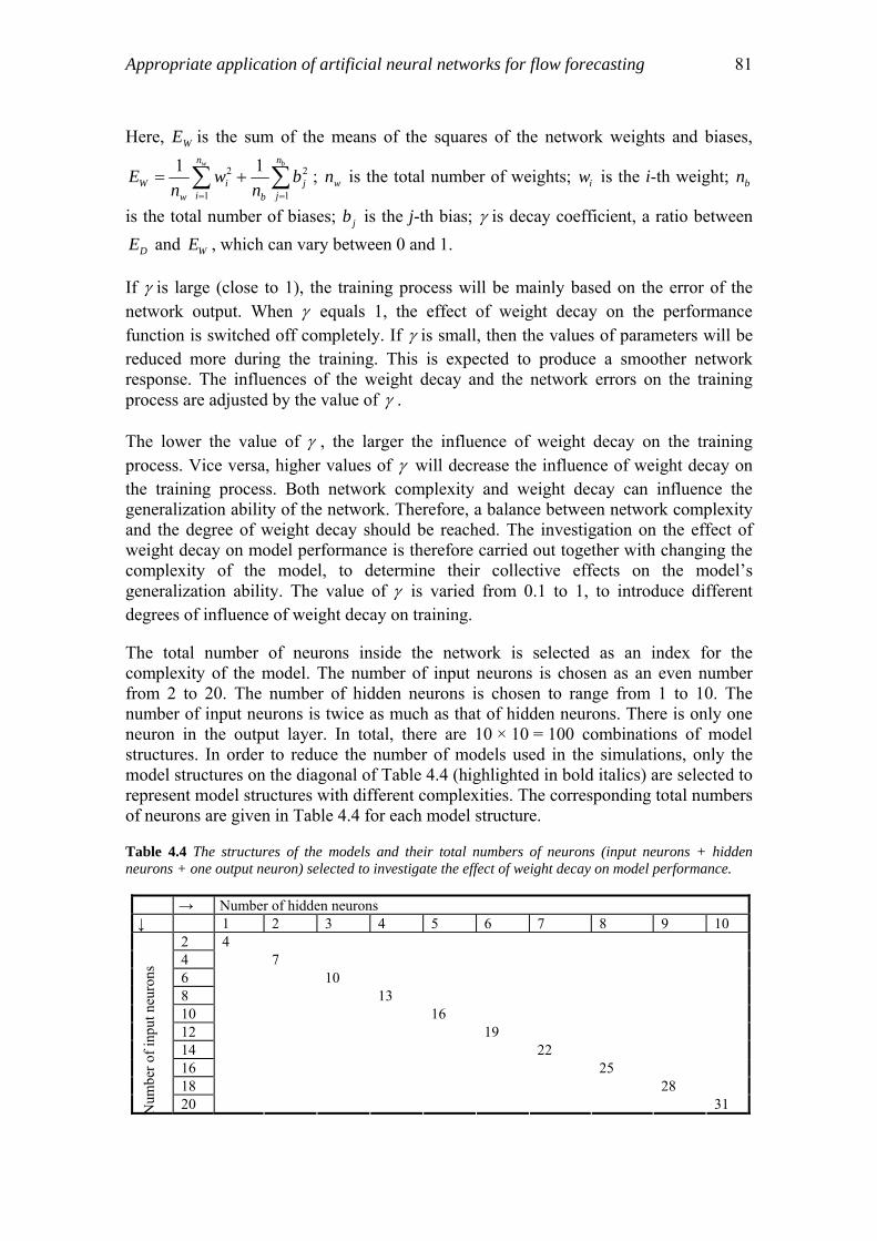
Appropriate application of artificial neural networks for flow forecasting 81

Here, is the sum of the means of the squares of the network weights and biases, WE

∑∑==

+=bw n

jj

b

n

ii

wW b

nw

nE

1

2

1

2 11 ; is the total number of weights; is the i-th weight;

is the total number of biases; is the j-th bias;

wn iw bn

jb γ is decay coefficient, a ratio between and , which can vary between 0 and 1. DE WE

If γ is large (close to 1), the training process will be mainly based on the error of the network output. When γ equals 1, the effect of weight decay on the performance function is switched off completely. If γ is small, then the values of parameters will be reduced more during the training. This is expected to produce a smoother network response. The influences of the weight decay and the network errors on the training process are adjusted by the value of γ .

The lower the value of γ , the larger the influence of weight decay on the training process. Vice versa, higher values of γ will decrease the influence of weight decay on the training process. Both network complexity and weight decay can influence the generalization ability of the network. Therefore, a balance between network complexity and the degree of weight decay should be reached. The investigation on the effect of weight decay on model performance is therefore carried out together with changing the complexity of the model, to determine their collective effects on the model’s generalization ability. The value of γ is varied from 0.1 to 1, to introduce different degrees of influence of weight decay on training.

The total number of neurons inside the network is selected as an index for the complexity of the model. The number of input neurons is chosen as an even number from 2 to 20. The number of hidden neurons is chosen to range from 1 to 10. The number of input neurons is twice as much as that of hidden neurons. There is only one neuron in the output layer. In total, there are 10 × 10 = 100 combinations of model structures. In order to reduce the number of models used in the simulations, only the model structures on the diagonal of Table 4.4 (highlighted in bold italics) are selected to represent model structures with different complexities. The corresponding total numbers of neurons are given in Table 4.4 for each model structure.

Table 4.4 The structures of the models and their total numbers of neurons (input neurons + hidden neurons + one output neuron) selected to investigate the effect of weight decay on model performance.

→ Number of hidden neurons ↓ 1 2 3 4 5 6 7 8 9 10

2 4 4 7 6 10 8 13 10 16 12 19 14 22 16 25 18 28

Num

ber o

f inp

ut n

euro

ns

20 31

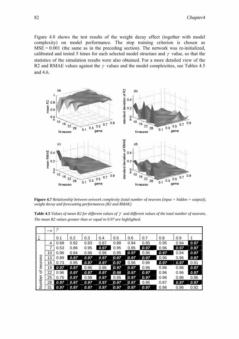
Chapter4 82

Figure 4.8 shows the test results of the weight decay effect (together with model complexity) on model performance. The stop training criterion is chosen as MSE = 0.001 (the same as in the preceding section). The network was re-initialized, calibrated and tested 5 times for each selected model structure and γ value, so that the statistics of the simulation results were also obtained. For a more detailed view of the R2 and RMAE values against the γ values and the model complexities, see Tables 4.5 and 4.6.

Figure 4.7 Relationship between network complexity (total number of neurons (input + hidden + output)), weight decay and forecasting performances (R2 and RMAE)

Table 4.5 Values of mean R2 for different values of γ and different values of the total number of neurons. The mean R2 values greater than or equal to 0.97 are highlighted.

→ γ

↓ 0.1 0.2 0.3 0.4 0.5 0.6 0.7 0.8 0.9 1 4 0.68 0.92 0.83 0.87 0.88 0.94 0.95 0.95 0.94 0.97 7 0.53 0.86 0.95 0.97 0.95 0.95 0.97 0.96 0.97 0.97

10 0.96 0.94 0.96 0.96 0.95 0.97 0.96 0.97 0.94 0.97 13 0.89 0.97 0.97 0.97 0.97 0.97 0.97 0.96 0.96 0.97 16 0.73 0.95 0.97 0.97 0.97 0.96 0.96 0.97 0.97 0.91 19 0.97 0.97 0.96 0.96 0.97 0.97 0.96 0.96 0.96 0.97 22 0.96 0.97 0.97 0.97 0.98 0.97 0.97 0.96 0.96 0.97 25 0.75 0.97 0.98 0.97 0.95 0.97 0.97 0.96 0.96 0.96 28 0.97 0.97 0.97 0.97 0.97 0.97 0.95 0.87 0.97 0.97

Num

ber o

f neu

rons

31 0.97 0.97 0.97 0.97 0.97 0.97 0.97 0.96 0.96 0.92

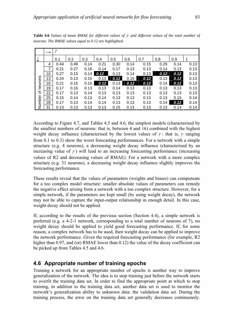
Appropriate application of artificial neural networks for flow forecasting 83

Table 4.6 Values of mean RMAE for different values of γ and different values of the total number of neurons. The RMAE values equal to 0.12 are highlighted.

→ γ

↓ 0.1 0.2 0.3 0.4 0.5 0.6 0.7 0.8 0.9 1 4 0.44 0.49 0.14 0.21 0.30 0.14 0.15 0.29 0.14 0.137 0.21 0.27 0.18 0.14 0.17 0.13 0.13 0.14 0.13 0.13

10 0.27 0.15 0.14 0.12 0.13 0.14 0.13 0.12 0.12 0.1313 0.24 0.13 0.15 0.13 0.12 0.15 0.12 0.13 0.12 0.1316 0.21 0.15 0.16 0.12 0.13 0.12 0.12 0.14 0.12 0.1319 0.17 0.16 0.13 0.13 0.14 0.13 0.13 0.13 0.13 0.1322 0.17 0.13 0.14 0.13 0.13 0.13 0.13 0.13 0.13 0.1325 0.15 0.14 0.13 0.14 0.13 0.13 0.13 0.13 0.15 0.1428 0.17 0.13 0.14 0.14 0.13 0.13 0.13 0.14 0.12 0.14

Num

ber o

f neu

rons

31 0.13 0.13 0.13 0.13 0.15 0.13 0.13 0.13 0.13 0.14

According to Figure 4.7, and Tables 4.5 and 4.6, the simplest models (characterised by the smallest numbers of neurons: that is, between 4 and 16) combined with the highest weight decay influence (characterised by the lowest values of γ : that is, γ ranging from 0.1 to 0.3) show the worst forecasting performances. For a network with a simple structure (e.g. 4 neurons), a decreasing weight decay influence (characterised by an increasing value of γ ) will lead to an increasing forecasting performance (increasing values of R2 and decreasing values of RMAE). For a network with a more complex structure (e.g. 31 neurons), a decreasing weight decay influence slightly improves the forecasting performance.

These results reveal that the values of parameters (weights and biases) can compensate for a too complex model structure: smaller absolute values of parameters can remedy the negative effect arising from a network with a too complex structure. However, for a simple network, if the parameters are kept small (by using weight decay), the network may not be able to capture the input-output relationship in enough detail. In this case, weight decay should not be applied.

If, according to the results of the previous section (Section 4.4), a simple network is preferred (e.g. a 4-2-1 network, corresponding to a total number of neurons of 7), no weight decay should be applied to yield good forecasting performance. If, for some reason, a complex network has to be used, then weight decay can be applied to improve the network performance. Given the required forecasting performance (for example, R2 higher than 0.97, and (or) RMAE lower than 0.12) the value of the decay coefficient can be picked up from Tables 4.5 and 4.6.

4.6 Appropriate number of training epochs Training a network for an appropriate number of epochs is another way to improve generalization of the network. The idea is to stop training just before the network starts to overfit the training data set. In order to find the appropriate point at which to stop training, in addition to the training data set, another data set is used to monitor the network’s generalization ability to unknown data: the validation data set. During the training process, the error on the training data set generally decreases continuously.

Chapter4 84

During the initial stage, the error on the validation data set will decrease too. When overfitting occurs, the training error will continue to decrease, but the validation error will start to increase. This point of change is a signal that the network starts to overfit. Therefore, as soon as the validation error starts to increase, the training of the network should stop. The aim of this section is to determine the effect of the number of training epochs on the forecasting performance. In addition to the training and validation data sets, a testing data set is used to test the final performance of the network.

Searching for an appropriate number of training epochs has to be done in combination with consideration of the network complexity. This can be explained as follows: for a simple network with very few neurons, training for many epochs may still not lead to overfitting, but for a complex network with many neurons, a low number of training epochs may already be enough to result in overfitting. Therefore, the effect of varying training epochs on forecasting performance is investigated in conjunction with varying model complexity, in terms of varying the total number of neurons. The number of training epochs ranges from 1 to 25. The network complexity is changed in a same way as that in the previous section (Section 4.5). Here, no weight decay is applied. Therefore, the performance function is MSE (or the value of γ is set to be 1) For each network structure, the training is repeated 10 times so as to obtain the mean of the model performance (mean R2 and mean RMAE). The effects of the training epochs and the model complexity on the forecasting performance are shown in Figure 4.8.

Appropriate application of artificial neural networks for flow forecasting 85

Figure 4.8 Effects of training epochs and model complexity on forecasting performance. 'N-neuron' is the total number of neurons in the network. 'Mean-R2' and 'mean RMAE' are the mean values of the two performance indices: Nash-Sutcliffe coefficient R2 and Relative Mean Absolute Error RMAE. 'Mean R2-train' is the mean R2 value calculated from the training data set; 'mean R2-validation' is the mean R2 value calculated from the validation data set; 'mean R2-test' is the mean R2 value calculated from the testing data set. The same idea applies to 'mean RMAE-train', 'mean RMAE-validation' and 'mean RMAE-test'.

In Figure 4.8, there are abnormally large (absolute) values of R2 and RMAE created from too simple network structures (with too few neurons). In order to exclude the influence of these large (absolute) values, two-dimensional plots are drawn from Figure 4.8 and shown in Figure 4.9 and 4.11. The R2 values shown are in the range from 0.6 to 1 and RMAE values in the range 0.1 to 0.3.

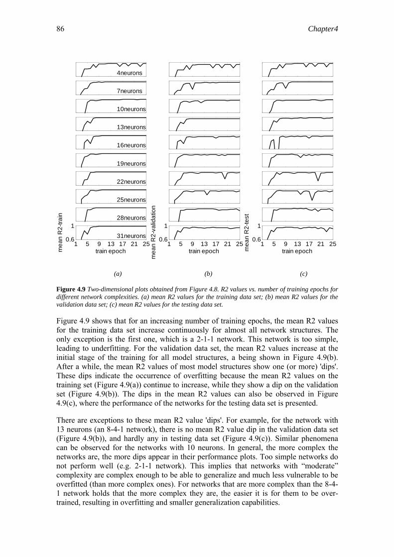
Chapter4 86

4neurons

7neurons

10neurons

13neurons

16neurons

19neurons

22neurons

25neurons

28neurons

1 5 9 13 17 21 250.6

131neurons

train epochmea

n R

2-tra

in

1 5 9 13 17 21 250.6

1

train epoch

mea

n R

2-va

lidat

ion

1 5 9 13 17 21 250.6

1

train epochmea

n R

2-te

st

(a) (b) (c)

Figure 4.9 Two-dimensional plots obtained from Figure 4.8. R2 values vs. number of training epochs for different network complexities. (a) mean R2 values for the training data set; (b) mean R2 values for the validation data set; (c) mean R2 values for the testing data set.

Figure 4.9 shows that for an increasing number of training epochs, the mean R2 values for the training data set increase continuously for almost all network structures. The only exception is the first one, which is a 2-1-1 network. This network is too simple, leading to underfitting. For the validation data set, the mean R2 values increase at the initial stage of the training for all model structures, a being shown in Figure 4.9(b). After a while, the mean R2 values of most model structures show one (or more) 'dips'. These dips indicate the occurrence of overfitting because the mean R2 values on the training set (Figure 4.9(a)) continue to increase, while they show a dip on the validation set (Figure 4.9(b)). The dips in the mean R2 values can also be observed in Figure 4.9(c), where the performance of the networks for the testing data set is presented.

There are exceptions to these mean R2 value 'dips'. For example, for the network with 13 neurons (an 8-4-1 network), there is no mean R2 value dip in the validation data set (Figure 4.9(b)), and hardly any in testing data set (Figure 4.9(c)). Similar phenomena can be observed for the networks with 10 neurons. In general, the more complex the networks are, the more dips appear in their performance plots. Too simple networks do not perform well (e.g. 2-1-1 network). This implies that networks with “moderate” complexity are complex enough to be able to generalize and much less vulnerable to be overfitted (than more complex ones). For networks that are more complex than the 8-4-1 network holds that the more complex they are, the easier it is for them to be over-trained, resulting in overfitting and smaller generalization capabilities.

Appropriate application of artificial neural networks for flow forecasting 87

4neurons

7neurons

10neurons

13neurons

16neurons

19neurons

22neurons

25neurons

28neurons

1 5 9 13 17 21 250.1

0.3 31neurons

train epochmea

n R

MA

E-tr

ain

1 5 9 13 17 21 250.1

0.3

train epoch

mea

n R

MA

E-v

alid

atio

n

1 5 9 13 17 21 250.1

0.3

train epochmea

n R

MA

E-te

st

(a) (b) (c)

Figure 4.10 Two-dimensional plots obtained from Figure 4.8. RMAE values vs. number of training epochs for different model complexities. (a) Mean RMAE values for the training data set; (b) mean RMAE values for the validation data set; (c) mean RMAE values for the testing data set.

Figure 4.10 reveals the effect of the number of training epochs on the mean RMAE values of the training, the validation and the testing data sets. Similar to the mean R2 values, the mean RMAE values for the training data set decrease continuously for an increasing number of training epochs. There are some disturbances on the mean RMAE values in the testing data set (Figure 4.10(c)) when the model becomes more and more complex (for a total number of neurons equal to 22, 25, 28 and 31).

According to the results shown in Figure 4.9 and 4.11, an 8-4-1 network (total number of neurons equal to 13) is selected as the appropriate network structure. The number of training epochs should be equal to or higher than 11 with MSE as its training performance function. Networks simpler than an 8-4-1network will lead to underfitting. The simpler the structure, the more likely underfitting is to happen. For the 4-2-1 network (7 neurons) and the 6-3-1 network (10 neurons), the number of training epochs should be equal to or higher than 13 to obtain a good forecasting performance. A too simple network (2-1-1) should not be used for its bad performance shown in Figure 4.9 and 4.11. Networks more complex than 8-4-1 will gradually lead to overfittting. More complex network will be overfitted earlier. For networks more complex than 8-4-1, a good performance can still be obtained if the number of training epochs is chosen carefully. According to Figures 4.10 and 4.11, a number of training epochs ranging from 8 to 11 results in good forecasting performance for these complex networks.

Chapter4 88

In Section 4.4, the 4-2-1 network was selected as the appropriate network structure under the condition that the effect of the training method on the network performance was not yet considered. Here, the 8-4-1 network is selected as the final appropriate network structure after an investigation of the combined effect of both network structure and training method on the network performance. According to the results presented in this section, both network structure and training method influence the network performance and they are mutually related. Therefore, they should be considered in combination with each other.

4.7 Discussion

4.7.1 The effectiveness of model complexity, weight decay and training epochs in preventing overfitting

Among the three measures used in this research to prevent overfitting in flow forecasting, choosing the appropriate network complexity is the most important, influential measure. According to Figure 4.9, the 8-4-1 network was considered to be the appropriate model structure among others investigated. This agrees roughly with the results presented in Table 4.2 where the appropriate training was not considered. The application of a validation data set to monitor the change of its model performance during the training course proves to be an effective way to determine the appropriate number of training epochs. Weight decay should be applied with caution: only in case the network is too complex.

4.7.2 The simplicity of discovered appropriate structure of ANN model According to Table 4.2, very simple networks perform very well. For example, a 4-2-1 network has only 2 non-linear and 1 linear equations, and has in total 13 parameters (10 weights and 3 biases) to model the rainfall-runoff process. The performance of this network stays high when trained with many epochs (up to 25, according to Figures 4.10(b) and (c)). The reasons why simple ANNs are able to model the rainfall-runoff process are: (1) the rainfall information is lumped for the whole study area, and (2) both rainfall and runoff information are lumped temporally to one day. Both lead to a significant depression of the variation of the rainfall-runoff process. In addition, consider the simplicity of the physics-based HBV model used in Chapter 3. The ANNs used here are reasonably simple and comparable to the HBV model.

4.8 Conclusions Over the past decade ANN-based flow forecasting models have been widely used because of their excellent representation in complex and non-linear function approximation. That does not mean that whenever an ANN model is set up and fed with training data sets, a perfect output will result automatically. Particular attention should be paid to maintain its generalization ability, and to prevent overfitting, which is likely to happen for such a modelling approach. This is usually done by trial-and-error which is fairly time-consuming and unreliable. Although overfitting is likely to take place, it can be restrained by careful selection of the model structure and control of the training procedures. This chapter recommends a systematic methodology to tackle this issue. During the implementation of the methodology the generalization capability of the

Appropriate application of artificial neural networks for flow forecasting 89

network is improved step by step. The methodology consists of three techniques: selecting the appropriate network structure, applying weight decay, and determining the appropriate number of training epochs. With regard to these three techniques used to prevent overfitting, the following conclusions can be drawn:

(1) Because of the random nature of the initialization, the network performance should be evaluated statistically. This can be done by training and testing the networks multiple times. This yields not only the means, but also the standard deviations of the performance indices (R2 and RMAE). The latter gives an indication of the uncertainties in the performance indices.

(2) Networks with moderate complexity (e.g. a network with an 8-4-1 structure) are robust in the sense that they are much less vulnerable to being overfitted (than both too complex ones and too simple ones).

(3) The values of parameters can compensate for the network complexity. For a simple network, weight decay is not a useful method to improve the network’s generalization ability. For a complex network, weight decay can help to prevent overfitting, by compensating the negative influence of a greater network complexity on the network performance.

(4) The appropriate number of training epochs is closely related to the network complexity. For the case studied here an 8-4-1 network trained for at least 11 epochs was identified as an appropriate network (with LM training algorithm, and no weight decaying being applied). Networks simpler than 8-4-1 should be trained more than 13 epochs. For networks more complex than 8-4-1, the appropriate number of training epochs ranges between 8 and 11.

(5) The network structure (or complexity) has the largest influence on the flow forecasting performance. The influence of the number of training epochs is somewhat smaller, and weight decay has the smallest influence on the flow forecasting performance.

Chapter4 90

Chapter 5

Discussion, conclusions and recommendations

5.1 Discussion

5.1.1 Objective-oriented approach The identification of the operational objective in a water resources project is important, because it guides the appropriate modelling process. For the water resources project studied here – the Geheyan Reservoir on the Qingjiang River – the main operational objective is maximum power generation. In order to maximize the power generated, forecasting of streamflow into the reservoir is necessary to optimize the water level and release. This optimization should be executed continuously and over a hydrological year (for large reservoirs, even for longer periods), so that the current and future benefits can be balanced to obtain maximum output. The lead time and indices to measure the forecasting accuracy on the long term (i.e., a hydrological year) are then appropriate measures of forecasting performance. The research described in this thesis used the Nash-Sutcliffe coefficient (R2), Relative Mean Absolute Errors (RMAE) and relative accumulated errors (RD) as (long-term) accuracy indices. A benefit analysis was used to determine explicitly the appropriate lead time and required values of R2 and RMAE.

If the main operational objective is not power generation, the modelling process will be oriented differently, resulting in different appropriate models. For example, if the main objective is flood defence, then forecasting of streamflow will not have to be continuous over a whole hydrological year, but can cover shorter periods during flooding seasons (seasonal or monthly forecasts). In that case, the streamflow forecasting becomes 'flood forecasting'. The peak discharge and the time-to-peak will be important variables to be forecasted. The index to measure the accuracy of peak discharge forecasting should be a short-term criterion, like the relative difference between forecasted and observed peak discharge. Another important quantity to forecast may be the volume of the peak for a certain duration (i.e., the 24 hours flooding volume), to help decide on the exact moment and quantity of storage water to be sluiced out, but forecasting the shape of the hydrograph will not be so important. If the specific flood defence objective is to minimize the flood damage related to the peak discharge at important cross sections of the river channel, then a 'flood damage evaluation' should be used to estimate the damage-forecasting performance relationships. Based on these relationships, the appropriate forecasting performance can be further identified.

In transforming the objective into required performance of streamflow forecasting, the potential benefits obtained from forecasting were analyzed. According to the results in chapter 2, if streamflow forecasting with a 4 days' lead time and an accuracy represented by an R2 value of 0.73 can be applied to optimize the reservoir operation, a 3% increase of the generated electricity with respect to what current actual operations

Chapter5 92

obtain (2.2×109 kW.h) can be achieved. To put the 3% into perspective, the increased amount of generated electricity is 6.6×107 kW.h, which equals 2.6 million euros on a yearly basis if the local price of electricity is about 0.04€/kW.h (Yu and An, 1999). If existing flow forecasting system cannot provide the required flow forecasting information, an improvement on the existing system will be necessary. This improvement will of course create financial costs. Therefore a cost analysis would be necessary to determine if the aforementioned benefits can balance the costs. For example, the costs arising from upgrading the data collection system, from adopting new models, etc. Because of a lack of information of the costs related to these issues, this cost analysis has not been performed in this study.

Based on the discussion in the previous paragraphs in this sub-section and the results obtained from chapter 2, 3 and 4, generic steps were formulated for the appropriate application of a model for a specific water management objective:

Figure 5.1 Generic steps taken to apply a selected model appropriately for a specific water management objective.

In applying these generic steps searching for appropriate models, three principles should be followed:

(1) An objective-oriented approach;

Discussion, conclusions and recommendations 93

(2) Follow the “principle of parsimony”: the model should be kept as simple as possible and extra components should be added only when necessary;

(3) The modelling steps should be consistent with each other.

5.1.2 Gains obtained from applying appropriate modelling concept in reservoir operation

Section 2.4 showed that if a perfect flow forecasting with zero forecasting error and a lead time of one year could be achieved, 3.0×109 kWh electricity could be generated in the hydrological year 1997, using the optimization method introduced in this study. This is regarded as the theoretical maximum benefit that could be obtained. In reality, 2.2×109 kWh electricity was actually generated in this hydrological year, i.e. 74% of the theoretical maximum benefit. The amount of generated electricity can be significantly increased, if a flow forecasting model is applied appropriately in optimizing the reservoir operation. For example, for flow forecasting with a lead time of 4 days, and an accuracy of 0.90 (in terms of the R2 value), 2.4×109 kWh electricity can be generated, an increase of 9% compared to the actual electricity generated. For the hydrological year 1997, a threshold lead time (33 days) was identified. Although this threshold lead time is not feasible with present flow forecasting technology, it is an indication of the theoretical upper limit of the extension of lead time of flow forecasting.

In applying a lumped HBV model, a very dense raingauge network may not be necessary. Chapter 3 showed that when five raingauges (out of the 26 existing raingauges in the study area) are used to perform flow simulation, the same model performance is achieved as for all 26 raingauges (i.e. a performance of 0.92 in terms of R2, see Figure 3.6). This implies that a reduction of the number of raingauges is possible, which will consequently result in a reduction of measurement costs and maintenance costs of the existing raingauge network.

In the application of ANNs for flow forecasting, overfitting and underfitting can be prevented by applying ANNs appropriately, i.e., by considering the modelling steps in combination and by making them consistent with each other.

5.1.3 Lead time This subsection explains why the lead times used in chapters 2, 3 and 4 are different.

In chapter 2, a 'threshold lead time' of 33 days was identified, which means that a further extension of the lead time beyond 33 days will not lead to significant further benefits. As a 33 days' lead time is not feasible for present streamflow forecasting techniques, a lead time of 4 days was selected to investigate the relationship between benefits and streamflow forecasting accuracy. The 4 days' lead time was calculated by summating the hydrological response time upstream of the Geheyan dam and the rainfall forecasting lead time in this area. As shown in chapter 3, the hydrological response time upstream of Yuxiakou is 18 hours. To estimate the hydrological response time upstream of Geheyan, which is 90 km downstream from Yuxiakou, the flood travelling time of this segment of the channel has to be added. According to Dai (2000, page 87), it is 4.5 hours; the hydrological response time upstream of the Geheyan dam then becomes 22.5 hours. For easy application of benefit analysis, it can be taken as 1

Chapter5 94

day. The lead time of the 'reliable' areally averaged rainfall provided by the local meteorological institute (Yichang Meteorological Observatory) is 3 days according to technicians at the Reservoir Regulation Center of the Qingjiang Hydropower Development Cooperation (pers. comm.). Therefore, a total of 4 days was taken as the feasible lead time for investigating the benefit-streamflow forecasting accuracy relationship in chapter 2.

If the ideal numbers of raingauges (five on certain locations) are used for real streamflow forecasting, the extension of the lead time of flow forecasting will not influence that number of raingauges much. This is because the appropriate setup of raingauges only influences the rainfall-runoff transformation process, which last for only 1 day. If the lead time of streamflow forecasting is more than 1 day, the error of the rainfall forecasting will be the dominant source of the error of the streamflow forecasting.

In chapter 3, instead of using forecasted rainfall series, observed rainfall series were used as input to the HBV model, which implies that there was no lead time at all. Instead of forecasting, the discharges were simulated with observed rainfall series in this case. The reason for that is to limit the source of error on the approximated areally averaged rainfall series to the spatial sampling strategy. The approximated areally averaged rainfall data were used to simulate the runoff; afterwards, the effects of the spatial sampling strategy on the rainfall-runoff transformation were identified. If forecasted rainfall series had been used, then – in addition to the error introduced by a less optimal spatial sampling strategy (fewer raingauges and at the wrong locations) – the forecasting error would also be introduced into the approximated areally averaged rainfalls. After the rainfall-runoff simulation, the effect of the spatial sampling strategy on the rainfall-runoff transformation will be blurred, because of the introduction of the un-related error – the forecasting error. Besides the errors introduced by different spatial sampling strategies and forecasting errors, there are other types of errors like measurement errors at raingauges and errors arising from the approximation method used to estimate the averaged rainfall. They are regarded as random and small errors, therefore were negligible.

In Chapter 4, a lead time of one day was chosen to study the appropriate application of a model based on an artificial neural network (ANN) for streamflow forecasting. This one day lead time is different form the lead time proposed in Chapter 2 (4 days). This is because a different river basin is used as case study in Chapter 4 (the Meuse River). Therefore, the lead time of flow forecasting is not necessarily the same as that in Chapter 2 (where Qingjiang River was taken as case study). However, the inconsistency of lead times could easily be removed by increasing the number of neurons in the output layer of the ANN model from 1 to 4, with the output of the first, second, third and fourth neuron representing the 1-, 2-, 3- and 4-days ahead forecasted discharge, respectively. The main structure of the model may have to be altered (e.g. by increasing the number of hidden neurons), because in this case the input-output relationship becomes more complex. The appropriate number of training iterations may also increase accordingly. Next, the required forecasting accuracy, derived - for example - from a benefit analysis (see Chapter 2), can be used to guide the appropriate application of ANN-based models.

Discussion, conclusions and recommendations 95

5.1.4 Accuracy and criteria The benefits obtained from streamflow forecasting generally increase with more accurate streamflow forecasting. No threshold like in the benefit-lead time relationship can be identified. Therefore, the identification of the appropriate accuracy of streamflow forecasting will depend on the managers’ preference on how much benefit they like to obtain, considering the costs and physical possibilities (of river basin and reservoirs) as well. This also applies to the identification of the appropriate lead time of streamflow forecasting. For the latter, the 'threshold lead time' first sets the upper limit of the range of the appropriate lead time. It is then further reduced by the physical constraints from rainfall forecasting and hydrological response time. Finally, the reservoir managers have to bring in their preference on appropriate lead time based on balance cost-benefit analysis.

A compromise also has to be reached between the extension of lead time and the increase of accuracy. Both lead to higher benefits. A careful evaluation of the benefits arising from these two indices of forecasting performance is necessary to determine which one is preferable. The relationship between the lead time and accuracy is also interesting. As can be intuitively foreseen, longer lead times will lead to a reduction in accuracy. Therefore, although streamflow forecasting with longer lead times will lead to higher benefits, the decreasing forecasting accuracy will have a negative effect on the benefits as well.

5.1.5 Model structure There are common issues to be considered when applying both the HBV and the ANN-based model for streamflow forecasting. Their data input should be appropriate, in terms of type of data, appropriate resolution of data, and the relationship between spatial and temporal resolution of the input data. For both models, the appropriate complexity should be determined. For the HBV model, aspects related to the model structure should be determined like the physical processes to be modelled, and the spatial and temporal resolution of these processes. For the ANN model, especially the 3-layer feed forward model used in this study, the model complexity was interpreted as the number of hidden neurons.

Calibration is also important for appropriate model performance. Model calibration is 'the procedure of adjustment of parameter values of a model to reproduce the response of reality within the range of accuracy specified in the performance criteria'. In most cases, models are calibrated based on historical data; therefore, the possibility exists that it might not be general enough for a new, unknown situation. This problem is less serious for physics-based models for the following two reasons. First, the generalization of unknown physical conditions (not being implied in historical data used for calibration) is considered in the embedded equations in the models. Secondly, most physics-based models are currently calibrated manually; the expertise used in the manual calibration will somehow prevent the model from being over-calibrated. For an ANN-based model, the over-calibration is so prone to happen that specific attention has to be paid to prevent it (like the measures described in chapter 4). This is because, first of all, very little physics was considered in the calibration, i.e., the calibration only depends on historical data. In the situation of extreme flooding beyond the range of historical records, the model functions like an extrapolation model to give the

Chapter5 96

corresponding response. As the physics behind extreme flooding events is different from that of normal hydrological conditions, this extrapolation does not match the real input-output transformation process. In this case, the physics-based model will give a more reasonable forecasting. Secondly, for the simplicity of ANN models, standard automatic calibration algorithms can be applied iteratively until the predefined accuracy criteria reached. For an ANN model, this is termed 'training'.

Automatic calibration methods are being developed for physics-based models (e.g., Zhang and Lindström, 1997). Because of the more complex structure of physics-based models (compared with ANN models), their application is still limited. With further development of automatic calibration methods for physics-based models, over-calibration may also start to become a problem. However, it may not be as serious a problem as with the ANN-based models, because the physics embedded in the model should be able to make the model more general.

5.1.6 The optimization period and reservoir Only one hydrological year (1997) was chosen for the benefit analysis, for the following reasons:

(1) Geheyan is designed as an annually operated reservoir. It is designed to complete a regulation cycle in a hydrological year: the water level starts to rise (from dead level) at the beginning of flooding season, should be at a maximum level at the beginning of the dry season and fall back to the dead level at the end of the dry season.

(2) It is possible that if the operation is optimized for periods longer than a year, higher benefits can be obtained, but it may neither affect the benefit-lead time relationship nor the benefit-accuracy relationship.

(3) There are risks associated with optimization for periods longer than a year. For example, the water level is kept too high at the beginning of the flooding season if the forecasting of the inflow in the forthcoming flooding season is underestimated. This can threaten the safety of the dam itself, which will never be made up by the extra benefits obtained from power generation. It is not likely that the reservoir operator would like to take this kind of risk.

If a different hydrological year is chosen to analyse the benefits obtained from streamflow forecasting, different amounts of benefit will be obtained. There was only one big flooding event in 1997. If a flooding event is larger in total volume and smaller in peak discharge – in other words, it is flatter than the 1997 one – more electricity will be generated. The 'threshold lead time' will also be different if the studied flooding event is different. Bigger floods (mainly in terms of total volume) will lead to longer 'threshold lead times'. If the flood is too big, the 'threshold lead time' will not extend any further because of the constraints of the beneficial (or active) storage of the reservoir, as shown in table 2.1.

Discussion, conclusions and recommendations 97

5.1.7 The studied basins Two river basins were used in this research: the Qingjiang River in China and the Meuse River in western Europe. The two basins were used for different types of models and different aspects in the modelling process. As the main purpose of the research described in this thesis is to demonstrate the methodology, not to identify the appropriate model for a specific basin, using different basins proves that the concept of appropriateness in model application is applicable to different river basins.

Table 5.1 lists the characteristics of the two river basins. Both river basins are rain-fed and fall into the same size category (although the Meuse basin is twice as big as Qingjiang) (Berger, 1992), but are very different in nature. Qingjiang is a mountainous basin, with steep river channel slopes and the hydrological response time is short. The temporal distribution of rainfall is very uneven: 76% of the rainfall is in its flood season (summer). In contrast, the Meuse River flows through a calm, relatively flat basin and the rainfall is more evenly distributed over the year. More importantly, because of these natural characteristics, these two rivers also have different functions. The main goals of managing the Qingjiang River are, in order of priority, power generation, flood defence, navigation, recreation, fishery, etc. For the Meuse River, they are water supply, navigation, ecology preservation, recreation, etc. (Booij, 2002, page 11). As a consequence, in contrast to the Qingjiang River, the Meuse River does not have many large reservoirs. The objective-oriented approach for finding the appropriate modelling approach for river basin management will lead to different appropriate models because of the different management objectives of these two basins, but the generic steps illustrated in Figure 5.1 apply to both basins.

Table 5.1 Comparison of the characteristics of the Qingjiang and Meuse Rivers

Characteristics Unit Qingjiang (upstream of Geheyan dam) (QHDC and CWRC, 1998)

Meuse (upstream of Borgharen) (Berger, 1992)

Source of runoff / Rain-fed Rain-fed Area km2 14 430 (page 33) 21 260 (page 118) Length of main channel km 361 (Dai, 2000, page 3) 631 (page 118) Average annual discharge at the interested cross-section m3/s 401 (page 33) 231 (page 118)

Average annual precipitation mm 1336 (page 22) 940 (page 118) Runoff coefficient / 0.62 (page 22) 0.43 (page 118) Mean slope of the river bed / 0.0018 (page 21) 0.00056 (page 16) Flooding (wet) season / summer winter Temporal variation of rainfall / 76% concentrated in wet

season (page 22) Evenly distributed in a year

Function of the river (in priority order) /

Power generation, flood defence, navigation, recreation, aqua production, etc.

water supply, navigation, ecology reservation, recreation, etc.

Chapter5 98

5.2 Conclusions How can benefit analysis for reservoir operation be carried out such that it produces performance requirements for streamflow forecasting?

The required lead time and accuracy of flow forecasting for improving hydropower generation of a reservoir were derived by simulating the benefits (in terms of electricity generated) obtained from forecasting with varying lead times and accuracies. The benefit-lead time relationship was investigated for perfect inflow forecasts only, with a few selected forecasting lead times: 4 days, 10 days and 1 year. The water level and release from the reservoir were then optimized. Based on the optimization results, a 'threshold' lead time (33 days) was identified, beyond which further extension of the forecasting lead time will not lead to significant further benefits. As the identified threshold lead time is not feasible for present streamflow forecasting techniques, a feasible lead time of 4 days was used to investigate the benefit-accuracy relationship. The 4 days' lead time was found by summing the hydrological response time (about 1 day) and the lead time of rainfall forecasting (3 days).

For streamflow forecasting with 4 days' lead time, the appropriate accuracy depends on the managers’ preference with regard to the benefit they intend to obtain from the streamflow forecasting. This is because the benefit obtained increases generally linearly with increasing level of accuracies, no threshold was identified like that in the benefit-lead time relationship. Therefore, for example, if an increase (of electricity generation) of 9% compared to the actual electricity (2.2×109 kWh) generated is expected, according to Figure 2.13, a flow forecasting with an accuracy of R2 value equal to 0.90 is required.

In addition, the linearly incremental relationship between the benefit and accuracy was very much dispersed. This implies that besides the quality of streamflow forecasting, there are other factors that also influence the benefits that can be obtained from streamflow forecasting.

For a physics-based model used for streamflow forecasting in a specific area, what is the appropriate spatial sampling of rainfall, which is an important aspect of model complexity, to fulfil the performance requirements?

Among all 26 raingauges existing in the studied area (the area upstream of the Yuxiakou of the Qingjiang River), 5 was proved to be enough to produce the same forecasting accuracy (in terms of e.g. R2 values) as that by using all 26 raingauges.

The geographical locations of these 5 raingauges were also identified. Most of them, 4 out of 5, are located in two tributaries (the Mashui and Zhongjian rivers), which contribute most (34%) of the discharge at the outlet of the studied area.

For a data-driven model used for streamflow forecasting in a specific area, what is the appropriate model structure, as it is one important aspect of model complexity, and the appropriate training method, as it is an example of model calibration, to produce the required performance?

As artificial neural networks are powerful tools for mapping the non-linear causal input-output relationships, the issue of preventing over-fitting (to the training data) and

Discussion, conclusions and recommendations 99

maintaining its generalization ability for new data is important and was selected as the topic for applying the appropriate modelling concept in ANN-based models. The selection of the number of input and hidden neurons, and the calibration (for ANN, termed 'training') are regarded as important modelling processes in tackling the problem of overfitting.

For the studied area (the area upstream of Borgharen of the Meuse River), and for a 1-day ahead flow forecasting, a 8-4-1 network was identified as an appropriate network structure. The 8 input neurons receive two types of inputs: 4-day ahead areally averaged rainfall records and 4-day ahead runoff records.

For the training algorithm used (Levenberg-Marquardt algorithm), the appropriate training epoch is 11 epochs (or more than that), without weight decay item in its performance function (for training).

Which generic steps can be taken to apply a selected model appropriately for a specific water management objective?

(1) Identify the water management objective explicitly. In this PhD project, the objective was defined as maximizing the hydropower generated from the reservoir.

(2) Select appropriate models. In this PhD project, they are the HBV model and an ANN-based model.

(3) Determine the required performance of the selected models for the specific water management objective. In this project, the appropriate lead time of flow forecasting is 4 days. The appropriate accuracy of this 4-day ahead flow forecasting depends on the manager’s preference on how much benefits do they intended to obtain: if an increase of electricity of 9% compared to the actual electricity (2.20×109 kWh) is favored, a 4-day ahead flow forecasting with an accuracy of R2 value equals to 0.90 will be required.

(4) Determine appropriate model complexity. The input, the structure of the model and the performance of the model output should be considered. As an example, in this project, the appropriate input data for a lumped HBV model was considered in chapter 3. In addition, the appropriate model complexity of ANN-based model was dealt with in chapter 4.

(5) Appropriate calibration of the model. The calibration process should be consistent with the complexity of the model. This was illustrated in chapter 4: the complexity of the network and the training of the network can be mutually compensated. For example, too simple networks will prone to be underfitted, this can be remedied by increase the training epochs, vice versa, too complex networks should not be training too much (the number of training epochs should be relatively smaller).

What can be gained from applying the appropriate modelling concept in water management?

The key idea of the appropriate model is that the complexity of the model should be just enough for its modelling objective. By applying the appropriate modelling concept in water management, no money will be spent on increasing the complexity when the complexity of the running model is already adequate or on increasing the complexity

Chapter5 100

beyond what is necessary. In this PhD research, although not all aspects of appropriate modelling process have been tackled, the following was gained:

(1) Extra electricity can be obtained. For example, if a 4 days ahead flow forecasting with an accuracy of R2 values equal to 0.90 is obtained and applied by using the optimization method introduced in this study, an increase of 9% electricity can be gained compared to the actual electricity (2.4×109 kWh) generated in the hydrological year 1997.

(2) For applying a lumped HBV model, a very dense raingauge network may not be necessary. For the partial area of the Qingjinag river basin studied in this research, 5 (among 26) raingauges are already enough to produce flow simulation as good as that with all raingauges being used. This has the potential to reduce the maintenance costs of the redundant raingauges.

(3) For the application of ANNs for flow forecasting, overfitting and underfitting can be prevented by applying them appropriately, e.g., by considering the modelling steps in combination with each other.

5.3 Recommendations

5.3.1 Input to the long-term optimization model The input for the long-term optimization model in this PhD research was the average monthly discharge as calculated from historical data. However, peak flooding events last only for about 10 days (see Figure 2.8(a)) and after having been averaged over a month, the peak discharge events will be smoothed out. Because of this smoothing out effect on the input, the long-term optimization model was unable to capture the biggest flood event in July of the year 1997 (as can be seen from Figure 2.8(c)), and no pre-releasing measure was taken to optimize the outcome. The benefits would be increased if the water level trajectory from the long-term optimization (which was used for guiding the short-term optimization procedure) could follow the optimal water level trajectory more closely. One possible way for this improvement, without any new information, is to use the 'annual hydrograph of daily observed discharge'. This hydrograph can be obtained by averaging the historical daily discharge on the same day over multiple years, with as many years of records involved as possible. In this case, the length of the optimization stage will be one day, but the optimization time horizon will be one year for the long-term optimization. The major point of introducing the 'annual hydrograph of daily observed discharge' is to estimate the magnitude and the timing of the hydrograph for every year. The benefit is that pre-releasing measures will also be taking place in the long-term optimization results, which should be able to guide the short-term optimization better.

5.3.2 Optimization algorithm The DP algorithm used in this PhD research discretized the whole state and decision spaces evenly and all states and decisions were considered in the backward recursion procedure to search the optimal decision series. This computation is time-consuming (one run of short-term optimization over one year takes about 50 minutes for an

Discussion, conclusions and recommendations 101

computer mounted with an Intel Pentium 4 CPU (2.66 GHz) and 1 GB RAM) and memory-consuming. A more efficient DP algorithm is recommended, so that the benefits-lead time-accuracy relationships (as shown in Figure 5.2) can be fully depicted. Examples of more efficient DP algorithms are: Incremental Dynamic Programming (IDP) (Nopmongcol and Askew, 1976), Discrete Differential Dynamic Programming (DDDP) (Nopmongcol and Askew, 1976) and Incremental Dynamic Programming with Successive Approximation (IDPSA) (Yakowitz, 1983). By using these algorithms, the same optimization results will be obtained, but the optimization procedure will be more efficient.

5.3.3 Appropriate temporal sampling of rainfall for flow simulation The relationship between the spatial and temporal sampling of rainfall remains to be identified, so that a balance between them can (and should) be reached. The following two aspects need to be considered in order to achieve such a balanced relationship (there are probably more):

(1) Which is more important in simulating the rainfall-runoff process, the temporal or the spatial sampling density?

(2) A balance between the spatial and temporal densities needs to be reached. If the improvement of one sampling density is not possible (or too costly), and if the rainfall-runoff simulation performance has to be improved, can we compensate by improving the other one?

Before identifying the spatial and temporal relationship of rainfall sampling, the appropriate temporal sampling of rainfall for flow simulation should be clarified. It is actually a problem of identifying the appropriate temporal sampling interval of rainfall. In order to be in line with the methodology used in chapter 3, the identification of the appropriate temporal sampling interval can also be carried out in two steps. First, the effect of the temporal sampling interval on the statistics of areally-averaged rainfall series will be identified. It can be expected that, by aggregating the rainfall over longer time intervals, the variability of the resulting areally-averaged rainfall series will be smoothed out. Secondly, the effect of the temporal sampling interval on the rainfall-runoff relationship will be identified. This effect can also be explored by using statistical methods and running a hydrological model. The appropriate temporal sampling of rainfall is also related to the spatial scale of the studied area, this will be discussed in following sub-section (5.1.4).

5.3.4 Relationship between rainfall sampling and model complexity The complexity of rainfall sampling (as input to the model) and the model itself should be compatible with each other, in order to diminish unnecessary costs and improve the performance of the model. In implementing the HBV model, the spatial resolution of the model, as one aspect of the model complexity, can be interpreted as the number of sub-basins to be divided for the studies area. The following aspects can be addressed in order to identify the relationship between the rainfall sampling complexity and the model complexity:

Chapter5 102

(1) The relationship between the spatial sampling density of rainfall and the model complexity (as discussed in section 3.8, more raingauges are necessary if the river basin is divided into multiple sub-basins);

(2) The relationship between the temporal sampling density of rainfall and the temporal resolution of model; normally they are unified to keep a consistency on the measuring interval of the input and output data;

(3) The relationship between the temporal sampling density of rainfall and the spatial resolution of model; for example, if the studied area is divided into sub-basins with large area, a dense temporal sampling on rainfall will not help to increase the modelled runoff, because of the big damping effect of the big sub-basin on the input – rainfall;

(4) A balance between the rainfall sampling complexity and the required quality of the runoff forecasting in the channel; the objective of using the runoff forecasting determines the quality of the runoff forecasting need to be reached, different objectives have different quality requirements; for a certain management objective which does not need high quality runoff forecasting, correspondingly, the rainfall sampling will not need to be complex.

The river basin, as a physical system, has a damping and filtering effect on the input (rainfall). Therefore, the variability of the runoff series is smaller than that of the rainfall series. Because of the damping and filtering effect, a very detailed sampling of rainfall may not have a recognizable effect on the runoff. Therefore, it is important to keep in mind that all the efforts are paid to improve the flow forecasting performance, not to master the rainfall regime. Any effort that cannot improve the flow forecasting performance is regarded as unnecessary extra work.

References

Abarbanel, H.D.I. (1996) Analysis of Observed Chaotic Data. Institute for Non-linear Science. New York, Springer-Verlag.

Abbott, M.B., Bathurst, J.C., Cunge, J.A., O’Connell, P.E. and Rasmussen, J. (1986) An introduction to the European Hydrological System- Système Hydrologique European, 'SHE.' 1: History and philosophy of a physically based distributed modeling system. J. Hydrol. 87, 45-59.

Abrahart, R.J., See, L. and Kneale, P.E. (1999) Using pruning algorithms and genetic algorithms to optimise network architectures and forecasting inputs in a neural network rainfall-runoff model. Journal of Hydroinformatics 1(2), 103-114.

An, G. (1996) The effects of adding noise during backpropagation training on a generalization performance. Neural Comput.8, 643-674.

Anmala, J., Zhang, B. and Govindaraju, R.S. (2000) Comparison of ANNs and Empirical Approaches for Predicting Watershed Runoff. J. Water Res. Plan. Manag. 126(3), 156-166.

Azimi-Zonooz, A., Krajewski, W. F., Bowles, D. S. and Seo, D. J. (1989) Spatial rainfall estimation by linear and non-linear co-kriging of radar-rainfall and raingauge data. Stochast. Hydrol. Hydraul. 3, 51–67.

Babovic, V. and Keijzer, M. (1999) Forecasting of river discharges in the presence of chaos and noise. In: Marsalek, J. (ed.), Coping with Floods: Lessons Learned from Recent Experiences. Kluwer, Dordrecht, The Netherlands.

Bárdossy, A. (2000) Fuzzy rule based flood forecasting, In: Bronstert, A., Bismuth, C. and Menzel, L. (eds.), European conference on advances in flood research. PIK report No.65, Postdam Institute of Climate Impact Research (PIK), 494-503.

Bartlett, P.L. (1997) For valid generalization, the size of the weights is more important than the size of the network. In: Mozer, M.C., Jordan, M.I. and Petsche, T. (eds.) Advances in Neural Information Processing Systems 9. MIT Press Cambridge, MA, USA, 134-140.

Bear, J. (1972) Dynamics of fluids in porous media. Dover Publications (Elsevier), New York, USA.

Becker, L. Yeh, W.W.-G., Fults, D. and Sparks, D. (1976) Operations models for central valley project, J. Water Res. Plan. Manag. April 1976, 101-115.

Bellman, B. (1957) Dynamic programming. Princeton University Press, Princeton, New Jersey, USA.

Berger, H.E.J. (1992) Flow forecasting for the river Meuse. PhD thesis. Delft University of Technology, Delft, The Netherlands.

Bergström, S. (1995) The HBV model. In: Singh, V.P. (ed.). Computer Models of Watershed Hydrology. Water Resources Publications, Colorado, USA, 443-476.

Beven, K. J. and Kirkby, M. J. (1979) A physically based, variable contributing area model of basin hydrology. Hydrolog. Sci. B. 24, 43-69.

Beven, K. (1989) Changing ideas in hydrology-the case of physically based models. J. Hydrol 105, 157-172.

Booij, M. J. (2002) Appropriate modeling of climate change impacts on river flooding. Ph.D thesis. University of Twente, Enschede, The Netherlands.

References 104

Bradley, A. A., Peters-Lidard, C., Nelson, B. R., Smith, J. A. and Young, C. B. (2002) Raingauge network design using Nexrad precipitation estimates. J. Am. Water Resour. Assoc. 38(5), 1393–1407.

Bras, R. L., Tarboton, D. G. and Puente, C. (1988) Hydrologic sampling—a characterization in terms of rainfall and basin properties. J. Hydrol. 102, 113–135.

Burgers, S.J., and Hoshi, K. (1978) Incorporation of forecasted seasonal runoff volumes into reservoir management. Water Resources Series Technical Report No. 58, 1978 November. Department of Civil and Environmental Engineering, University of Washington, Seattle, Washington, USA.

Campolo, M., Andreussi, P. and Soldati, A. (1999) River flood forecasting with a neural network model. Water Resour. Res. 35(4), 1191-1197.

Coulibaly, P., Andtil, F. and Bobée, B. (2000) Daily reservoir inflow forecasting using artificial neural networks with stopped training approach. J. Hydrol. 230, 244-257.

Dai, G. (2000) Hydraulic structures and reservoir operation: series of training textbooks of Geheyan hydropower plant. Press of Wuhan University of hydraulic and electric engineering, Wuhan, China (in Chinese).

De Kok, J.L., Van der Wal, K. and Booij, M.J. (2004) Appropriate accuracy of models for decision support systems: Case example for the Elbe River basin. In: Pahl-Wostl, C., Schmidt, S., Rizzoli, A.E. and Jakeman, A.J. (eds) Complexity and Integrated Resources Management, Transactions of the 2nd Biennial Meeting of the International Environmental Modelling and Software Society, Volume 2, 1021-1026.

Dong, X. and Vreugdenhil, C.B. (2002) Balancing between generalization and over-fitting: ANN-based modelling for flow forecasting. Proceedings of second international symposium on flood defence (ISFD’2002), Beijing, China, 892-900.

Duncan, M. R., Austin, B., Fabry, F. and Austin, G. L. (1993) The effect of gauge sampling density on the accuracy of streamflow prediction for rural catchments. J. Hydrol. 142, 445–476.

Ette, E.I., Williams, P.J., Kim, Y.H., Lane, J.R., Liu, M.J. and Capparelli, E.V. (2003) Model appropriateness and population pharmacokinetic modeling. J Clin.Pharmacol. 43(6), 610-623.

Feldman, A.D. (1995) HEC-1 flood hydrograph package. In: Singh, V.P. (ed.). Computer Models of Watershed Hydrology. Water Resources Publications, Colorado, USA, 119-150.

Foresee, F.D., and Hagan, M.T. (1997) Gauss-Newton approximation to Bayesian regularization. Proceedings of the 1997 International Joint Conference on Neural Networks, 1930-1935.

Fujita, O. (1998). Statistical estimation of the number of hidden units for feedforward neural networks. Neural Networks 11, 851-859.

Funahashi, K.I. (1989) On the approximate realization of continuous mappings by neural networks. Neural Networks 2, 183-192.

Geoffrion, A.M. (1976) The purpose of mathematical programming is insight, not numbers. Interfaces 7(1), 81-92

Georgakakos, A.P. and Marks, D.H. (1987) A new method for the real-time operation of reservoir systems. Water Resour. Res. 23(7), 1376-1390.

References 105

Georgakakos, A.P. (1989) The value of streamflow forecasting in reservoir operation. Water Resour. Bull. 25(4): 789-800.

Georgakakos, K. P., Bae, D. H. and Cayan, D. R. (1995) Hydroclimatology of continental watersheds: 1. temporal analyses. Water Resour. Res. 31(3), 655–675.

Govindaraju, R.S. and Ramachandra Rao, A. (eds.) (2000) Artificial neural networks in hydrology. Water Science and Technology Library, Vol. 36 Kluwer Academic Publishers, Dordrecht, The Netherlands.

Hagan, M.T., Demuth, H.B. and Beale, M. (1996) Neural Network Design. PWS Publishing Company, Boston, MA, USA.

Hall, W.A. and Dracup, J.A. (1970) Water Resources Systems Engineering. McGraw Hill, New York, USA.

Hamlet, A.F. and Lettenmaier, D.P. (1999) Columbia river streamflow forecasting based on ENSO and PDO climate signals. J. Water Resour. Plan. Management 125(6), 333-341.

Hamlet, A.F., Huppert, D. and Lettenmaier, D.P. (2002) Economic value of long-lead streamflow forecasts for Columbia river hydropower. J. Water Resour. Plan. Management 128(2), 91-101.

Haykin, S. (1999) Neural Networks: a Comprehensive Foundation. 2nd ed., Prentice Hall, Inc., New Jersey, USA.

Holmströn, L. and Koistinen, P. (1992) Using additive noise in back-propagation training. IEEE T. Neural Network. (3) 24-38.

Hornberger, G.M and Spear, R.C. (1980) Eutrophication in peel inlet, П, identification of critical uncertainties via generalised sensitivity analysis. Water Res., 14, 43-49.

Hornberger, G.M. and Spear, R.C. (1981) An approach to the preliminary analysis of environmental systems. J. Environ. Management 12, 7-18.

Hornik, K. (1991) Approximation capabilities of multilayer feedforward networks. Neural Networks 4(2), 251-257.

Hornik, K., Stinchcombe, M., and White, H. (1989) Multilayer feedforward networks are universal approximators. Neural Networks 2, 359-366.

HSCSC (Hubei Science Consultant Service Centre) (1991) The Consultant Report for the Development of Qingjiang River Basin. Hubei, China (in Chinese).

http://www.irn.org/programs/china/. International Rivers Network. Accessed on 9 May 2005.

http://www.smhi.se/foretag/m/hbv_demo/html/welcome.html. Swedish Meteorological and Hydrological Institute. Accessed on 3 May 2005.

Imrie, C.E., Durucan, S. and Korre, A. (2000) River flow prediction using artificial neural networks: generalisation beyond the calibration range. J. Hydrol. 233, 138-153.

Jain, S.K., Das, A. and Srivastava, D.K. (1999) Application of ANN for Reservoir Inflow Prediction and Operation. J. Water Resour. Plan. Management 125(5), 263-271.

Jakeman, A.J. and Hornberger, G.M. (1993) How much complexity is warranted in a rainfall-runoff model? Water Resour. Res. 29, 2637-2649.

Jolley, T.J. (1995) Large-scale hydrological modelling - the development and application of improved land-surface parameterisations for meteorological models. PhD thesis, Imperial College of Science, Technology and Medicine, London, UK.

References 106

Karamouz, M., Szidarovszky, F. and Zahraie, B. (2003) Water Resources Systems Analysis. Lewis Publishers, USA.

Kite, G. W. and Kouwen, N. (1992) Watershed modelling using land classifications. Water Resour. Res. 28, 3193-3200.

Koistinen, P. and Holmströn, L. (1992) Kernel regression and backpropagation training with noise. NIPS4 1033-1039.

Kraijenhoff van de Leur, D.A. (ed). (1986) River flow modeling and forecasting. D. Reidel Publishing Company, Dordrecht, The Netherlands.

Krajewski, W. F., Lakshmi, V., Georgakakos, K. P. and Jain, S. C. (1991) A Monte Carlo study of rainfall sampling effect on a distributed catchment model. Water Resour. Res. 27(1), 119–128.

Krogh, A. and Hertz, J.A. (1992) A simple weight decay can improve generalization. In: Moody, J.E., Hanson, S.J. and Lippmann, R.P. (eds.) Advances in Neural Information Processing Systems 4. Morgan Kaufmann Publishers Inc., San Mateo, CA, USA, 950-957

Larson, R.E. and Casti, J.L. (1978) Principles of Dynamic Programming, Part 1: Basic Analytic and Computational Methods. Marcel Dekker Inc., New York and Basel.

Laurenson, E.M. and Mein, R.G. (1995) RORB: hydrograph synthesis by runoff routing. In: Singh, V.P. (ed.) Computer Models of Watershed Hydrology, Water Resources Publications, Colorado, 151-164.

Leavesley, G.H. and Stannard, L.G. (1995) The precipitation-runoff modelling system-PRMS. In: Singh, V.P. (ed.). Computer Models of Watershed Hydrology. Water Resources Publications, Colorado, USA, 281-310.

Lee, B.L. (1973) Requiem for large-scale models. J. Amer. Inst. Planners 39, 163-178. Legates, D.R. and McCabe Jr., G.J. (1999) Evaluating the use of 'goodness-of-fit'

measures in hydrologic and hydroclimatic model validation. Water Resour. Res. 35(1), 233-241.

Lindström, G., Johansson, B., Persson, M., Gardelin, M. and Bergström, S. (1997) Development and test of the distributed HBV-96 hydrological model. J. Hydrol. 201, 272–288.

Linsley, R. K., Kohler, M. A. and Paulhus, J. L. H. (1988) Hydrology for Engineers. McGraw-Hill, London, UK.

Linsley, R.K., Franzini, J.B., Freyberg, D.L. and Tchobanoglous, G. (1992) Water-resources Engineering, McGraw-Hill Inc., New York, USA.

Loague, K.M. and Freeze, R.A. (1985) A comparison of rainfall-runoff modelling techniques on small upland catchments. Water Resour. Res. 21(2), 229-248.

Lovejoy, S. and Schertzer, D. (1985) Generalized scale invariance in the atmosphere and fractal models of rain. Water Resour. Res. 21, 1233-1250.

MacKay, D.J.C. (1992) Bayesian interpolation. Neural Comput.4(3), 415-447. Maidment, D.R. (1992) Handbook of Hydrology. McGraw-Hill Inc., New York, USA. Minns, A.W., and Hall, M.J. (1996) Artificial neural networks as rainfall-runoff models.

Hydrol. Sci. J. 41(3), 399-417. Moody, J.E. (1992) The effective number of parameters: an analysis of generalization

and regularization in nonlinear learning systems. In: Moody, J.E., Hanson, S.J. and Lippmann, R.P. (eds.) Advances in Neural Information Processing Systems 4. Morgan Kaufmann Publishers Inc., San Mateo, CA, USA, 847-854.

References 107

Morris, E.M. (1980) Forecasting flood flows in grassy and forested basins using a deterministic distributed mathematical model. IAHS Publication 129, Wallingford, UK, 247-255.

Moussa, R. and Bocquillon, C. (1996) Criteria for the choice of flood-routing methods in natural channels. J. Hydrol. 186, 1-30.

Nash, J. E. and Sutcliffe, J. V. (1970) River flow forecasting through conceptual models, Part 1-A discussion of principles. J. Hydrol. 10, 282-290.

Nelson, M.C. and Illingworth, W.T. (1991) A Practical Guide to Neural Nets. Addison-Wesley, Reading, MA, USA.

Nikora, V. I. (1994) Self-similarity and self-affinity of drainage basins. Water Resour. Res. 30, 133-137.

Nopmongcol, P. and Askew, A.J. (1976) Multilevel incremental dynamic programming. Water Resour. Res. 12(6), 1291-1297.

Osborn, T. J. and Hulme, M. (1997) Development of a relationship between station and grid-box rain day frequencies for climate model evaluation. J. Climate 10, 1885–1908.

Passchier, R.H. (1996) Evaluation hydrologic model packages, Q2044. WL|Delft Hydraulics, Delft.

Penman, H.L. (1949) The dependence of transpiration on weather and soil conditions. J. Soil Sci. 1, 74–89.

QHDC (Qingjiang Hydropower Development Corporation-Reservoir Regulation Center) and CWRC (Changjiang Water Resources Committee-Department of Planning) (eds.), 1998. Regulation rules of Geheyan reservoir-Qingjiang, Hubei, China. (in Chinese).

Quick, M.C. (1995) The UBC watershed model. In: Singh, V.P. (ed.) Computer Models of Watershed Hydrology. Water Resources Publications, Colorado, USA, pp.233-280.

Raman, H., Sunilkumar, N. (1995) Multivariate modeling of water resources time series using artificial neural networks. J. Hydrol. Sci. 40 (2), 145-163.

ReVelle, C., Joeres, E. and Kirby, W. (1969) The linear decision rule in reservoir management and design: 1. Development of the stochastic model. Water Resour. Res. 5(4), 767-777.

Robinson, J. (1976) Useless for any practical purpose, Econ. Polit. Weekly XI(9), 361-363.

Rodriguez-Iturbe, I. and Mejia, J. M. (1974) On the transformation from point rainfall to areal rainfall. Water Resour. Res. 10, 729–735.

Rogers, P. (1978) On the choice of the 'appropriate model' for water resources planning and management. Water Resour. Res. 14(6), 1003-1010.

Sajikumar, N. and Thandaveswara, B.S. (1999). A non-linear rainfall-runoff model using an artificial neural network, J. Hydrol. 216, 32-55.

Saloranta, T.M., Kämäri, J., Rekolainen, S. and Malve, O. (2003) Benchmark Criteria: A Tool for Selecting Appropriate Models in the Field of Water Management. Environ. Management 32(3), 322 – 333.

Seibert, J. (1999) Regionalisation of parameters for a conceptual rainfall–runoff model. Agric. For. Met. 98–99, 279–293.

Sharkey, A.J.C. (1996) On Combining Artificial Neural Nets. Connect. Sci.8(3-4), 299-314.

Sharkey, A.J.C. (1999) Combining Artificial Neural Nets: Ensemble and Modular Multi-Net Systems. Springer, London, UK.

References 108

Sivapalan, M., Beven, K. J. and Wood, E. F. (1990) On hydrologic similarity: 3. A dimensionless flood frequency model using a generalized geomorphologic unit hydrograph and partial area runoff generation. Water Resour. Res. 26, 43-58.

SMHI (2003) Integrated hydrological modelling system (IHMS) HBV Manual Version 4.5. Swedish Hydrological and Hydrological Institute, Norrköping, Sweden.

Smith, J. (1996) Models and scale: up- and downscaling. In: Stein, A., Penning de Vries, F. W. T. and Schotma, P. J. (eds.), Models in Action, Proceedings of a seminar series 1995-1996, Wageningen, 25-41.

Speers, D.D. (1995) SSARR model. In: Singh, V.P. (ed.). Computer Models of Watershed Hydrology. Water Resources Publications, Colorado, USA, 367-394.

Stallings, E.A. and Fread, D.L. (1998) The benefit of hydrological forecasting. WMO bulletin 47 (1), 61-63.

St-Hilaire, A., Ouarda, T. B. M. J., Lachance, M., Bobée, B., Gaudet, J. and Gignac, C. (2003) Assessment of the impact of meteorological network density on the estimation of basin precipitation and runoff: a case study. Hydrol. Processes 17(18), 3561–3580.

Stüber, M., Gemmar, P. and Greving, M. (2000) Machine supported development of fuzzy-flood forecast systems. In: Bronstert, A., Bismuth, C. and Menzel, L. (eds.) European conference on advances in flood research. PIK report No.65, Postdam Institute of Climate Impact Research, 504-515.

Sugawara, M. (1995) Tank model. In: Singh, V.P. (eds.). Computer Models of Watershed Hydrology. Water Resources Publications, Colorado, USA, 165-214.

Taniguchi, M., and Tresp, V. (1997) Averaging regularized estimators. Neural Comput.9, 1163-1178.

Tarboton, D. G., Bras, R. L. and Puente, C. E. (1987) Combined hydrologic sampling criteria for rainfall and streamflow. J. Hydrol. 95, 323–339.

Thorburn, W.M. (1915) Occam’s razor. Mind 24(94), 287-288. Thorburn, W.M. (1918) The myth of Occam’s razor. Mind 27(107), 345-353. Tokar, A.S. and Johnson, P.A. (1999) Rainfall-runoff modeling using artificial neural

networks. J. Hydrol. Engng. 4(3), 232-239. Tsintikidis, D., Georgakakos, K. P., Sperfslage, J. A., Smith, D. E. and Carpenter, T. M.

(2002) Precipitation uncertainty and raingauge network design within Folsom Lake watershed. J. Hydrol. Engng. 7(2), 175–184.

Vreugdenhil, C.B. (2002) Accuracy and Reliability of Numerical River Models J. Am. Water Resour. As. 38(4), 1083-1095.

Wagener, T. and Wheater, H. S. (2001) A generic framework for the identification of parsimonious rainfall-runoff models. In: Rizzoli, A.E. and Jakeman, A.J. (eds.) Integrated Assessment and Decision Support, Proceedings of the 1st Biennial Meeting of the iEMS.

Wagener, T., Boyle, D. P. Lees, M. J. Wheater, H. S., Gupta, H. V. and Sorooshian, S. (2001) A framework for development and application of hydrological models. Hydrol. Earth System Sci. 5(1), 13–26.

Wagener, T., McIntyre, N., Lees, M. J., Wheater, H. S. and Gupta, H. V. (2003) Towards reduced uncertainty in conceptual rainfall-runoff modelling: Dynamic identifiability analysis. Hydrol. Process. 17, 455–476.

Weigend, A. (1994) On overfitting and the effective number of hidden units. Proceedings of the 1993 Connectionist Models Summer School, 335-342.

Western, A. W. and Blöschl, G. (1999) On the spatial scaling of soil moisture. J. Hydrol. 217, 203–224.

References 109

Wood, E. F., Sivapalan, M., Beven, K. and Band, L. (1988) Effects of spatial variability and scale with implications to hydrologic modelling. J. Hydrol. 102, 29-47.

Yakowitz, S.J. (1983) Convergence rate analysis of the state increment dynamic programming method. Automatica 19(1), 53-60.

Yeh, W.W.G., Becker, L., Cohn, M.J. and Zettlemoyer, R. (1980) Benefits of long-range streamflow prediction. Contribution No. 181, California Water Resources Center, University of California, Davis, CA, USA.

Yeh, W.W-G., Becker, L. and Zettlemoyer, R. (1982) Worth of flow forecast for reservoir operation. J. Water Res. Plan. Manag. 108, 257-269.

Yeh, W.W-G., Sohn, R.L. and Becker, L. (1978) Information requirements for improving hydropower. J. Water Res. Plan. Manag. 104(1), 139-156.

Yevjevich, V. (1972) Probability and Statistics in Hydrology. Water Resources Publications, Littleton, Colorado, USA.

Yu, W. and An, Y. (1999) Rolling development of Qingjiang basin. China Three Gorges Construction 7(48) (in Chinese).

Zealand, C.M., Burn, D.H, Simonovic, S.P. (1999) Short term streamflow forecasting using artificial neural networks. J. Hydrol. 214, 32–48.

Zhang, X. and Lindström, G. (1996) A comparative study of a Swedish and a Chinese hydrological model. Water Resour. Bull. 32(5), 985–994.

Zhang, X. and Lindström, G. (1997) Development of an automatic calibration scheme for the HBV hydrological model. Hydrol. Processes 11(12), 1671-1682.

Zhao, R.J. and Liu, X.R. (1995) The Xinanjiang model. In: Singh, V.P. (eds.). Computer Models of Watershed Hydrology, Water Resources Publications, Colorado, USA, 215-232.

Zhou, Z., Shen, Z., Shi, X. and Li, T. (1997) Water Resources and Hydropower Planning, second edition, China Water Power Press, Beijing, China (in Chinese).

References 110

List of symbols

jb the j-th bias

),( ttt RHb the immediate stage benefit obtained from releasing discharge from reservoir at stage t, with reservoir water level being

tR

tH

),,( tttt RQHb the immediate stage benefit obtained at stage t, when inflow to the reservoir is , release from the reservoir is , and the reservoir water level is

tQ tR

tH

),( ttt xsb the immediate stage benefit obtained from making decision at stage t tx

B benefit matrix

maxB maximum overall benefit

)( tt HB the benefit obtained from executing the optimal policy from stage t to final stage T, with Ht being the initial state

)( 11 ++ tt HB the optimal sub-policy benefit obtained from a series of decisions starting from stage t+1 and ending at the final stage T

)( 11 ++ TT HB the terminal benefit obtained after the application of the last decision, when the terminal state at the end of the last stage is reached

),( ,11,1 tt PSB sub-policy benefit accumulated over stages from the first stage up to stage t, with as the initial stage, and the decision series (sub-policy)

1s tp ,1

),( ,11,1∗TT PSB optimal policy benefit accumulated over all stages from the first stage up

to the final stage T, based on the initial stage and optimal policy 1s∗

Tp ,1

cov(xi, yi+k) the covariance between time series xi and yi for lag time k

2nC the number of combinations of 2 raingauges among n

e a vector of network errors

DE mean square error

fE firm energy, tNE ff ∆⋅=

List of symbols 112

tE electricity generated at time t (kWh)

WE the sum of the means of the squares of the network weights and biases

f the underlying input-output function of a system

)(HfSH reservoir storage-water level relationship

1f hyperbolic tangent sigmoid transfer functions

2f linear transfer functions

g acceleration of gravity, g = 9.81m/s2

kg the gradient at iteration k

th tail-water level during stage t

th average tail-water level during stage t

tH reservoir water level at the beginning of stage t

tH average reservoir water level during stage t

tHe Heaviside unit step function, ⎩⎨⎧

<≥

=NfNNfN

Het

tt ,1

,0

Hinit(t) initial state (water level) of one short-term optimization cycle t

Hterm(t) terminal conditions for each short-term optimization cycle, interpolated from long-term optimization results

ip the number of past outputs

iq the number of past inputs

I the identity matrix

J the Jacobian matrix that contains the first derivatives of the network errors with respect to the weights and biases

TJ transferred Jacobian matrix

k time lag for calculating the lagged cross-correlation coefficient

MSE mean squared error

n number of raingauges

List of symbols 113

bn the total number of biases

wn the total number of weights

N the total number of training data sets

fN firm power, MWN f 180=

tN power output at stage t, kW

p input to artificial neural networks

)(tP rainfall measured at time t

tjiP ,, an individual element of a three-dimensional state transformation matrix, which means that, at stage t, starting with state i, after the implementation of decision j, the state will reach the value saved in tjiP ,,

tP the state transfer function of stage t

tP ,1 a sub-policy including a series of decisions made from stage 1 to t

*,1 tP optimal policy benefit

tPspace +1 the decision space from stage 1 to t

tQ recorded flow to at time t (m3/s)

'tQ modelled flow to the reservoir during stage t (m3/s)

tQ the mean of observed flow series

ijr the sample product–moment correlation coefficient between rainfall series of gauges i and j

r the arithmetic mean of the correlation coefficients of all bi-combinations of the raingauges

Rk the expected cross-correlation coefficient for lag time k

maxR maximum release permitted to the downstream of the reservoir (m3/s)

minR minimum release to the downstream required by navigation, irrigation, water supply, creation, fishing, wild life protection, etc.

List of symbols 114

spaceR decision space of reservoir

Rt total release from the reservoir at time t (m3/s)

RD relative accumulated difference between computed and observed discharge

Remax maximum release permitted through turbine (m3/s)

Remin minimum release permitted through turbine (m3/s)

tRe release through turbine at time t (m3/s)

RMAE relative mean absolute error

R2 Nash-Sutcliffe coefficient

2s the variance of the areally averaged rainfall

2js the variance of the j-th raingauge

2xs the variance of the areally averaged rainfall series x

2ys the variance of the discharge series y

2js the mean of the station variance

spaceS feasible state space

tS the state of the system at stage t, also referred as the reservoir storage at stage t (m3)

t time or stage

T state transition matrix

Td the total duration of the pre-releasing and refilling periods

Tl lead time of flow forecasting

Tlthreshold the threshold lead time

var xi the variance for series xi

var yi+k the variance for series yi+k

iw the i-th weight

List of symbols 115

ix areally averaged rainfall measured at time i

ijx the rainfall recorded at the i-th time point and the j-th raingauge

x mean areally averaged rainfall

jx the mean of the j-th raingauge

kx vector of weights and biases of the training iteration k

tXspace feasible decision space of stage t

tX decision made at stage t

iy discharge measured at time i

y mean discharge

α autocorrelation coefficient of the forecasting error series: tt QQ −'

kα the learning rate

tβ noise added to the observed flow series

γ decay coefficient used ot modify the performance function in training ANNs; it is a ratio between and , which can vary between 0 and 1 DE WE

tδ scaling factor drawn from a random uniform distribution in the interval [-1, +1]

t∆ length of the stage

tε random number, normally distributed with zero mean and unit variance

η the efficiency of the hydropower plant, 866.0321 == ηηηη ; 1η is the efficiency of turbines; 2η is the efficiency of generators; 3η is the efficiency of transmission mechanisms; η is a varying efficient according to the net water head and the discharge through the turbine,

[ tRhHf ),( −= ]η . Here a constant empirical value (0.866) is taken for such a large-scale (total installed capacity greater than 250MW) hydropower plant, according to the recommendation of Zhou et al. (1997, p106)

µ the Marquardt parameter introduced to adjust the convergence rate

List of symbols 116

ν penalty factor, ν = 0.4

ϕ an assumed absolute deviation from as normalized with respect to , tQ tQ

ttt QQQ /' −=ϕ

Appendix

Indices to measure the accuracy of flow forecasting

Nash-Sutcliffe coefficient-R2

( )

( )∑

∑

=

=

−

−−= N

ttt

N

ttt

QQ

QQR

1

2

1

2'

12 (A.1)

where is the synthesized flow at time t; is the observed flow at time t; N is the

total number of observations;

'tQ tQ

tQ is the mean of observed flow series. (Nash and Sutcliffe, 1970). The value of R2 ranges from –∞ to 1, the higher the value, the better the agreement between computed and observed discharges.

Relative Mean Absolute Error-RMAE

∑

∑

=

=

−= N

tt

N

ttt

Q

QQRMAE

1

1

'

(A.2)

The meaning of the symbols is the same as that of the definition of R2 (Maidment, 1992).

Relative accumulated difference between computed and observed discharge-RD

( )

∑

∑

=

=

−= N

tt

N

ttt

Q

QQRD

1

1

'

(A.3)

The meaning of the symbols is the same as that of the definition of R2 (Maidment, 1992). The relative accumulated difference, RD is used to identify any bias in the water balance, which is particularly useful in the initial stage of the calibration.

Appendix 118

Mean Squared Error-MSE

(∑=

−=N

ttt QQ

NMSE

1

2'1 ) (A.4)

The meaning of the symbols is the same as that of the definition of R2 (Maidment, 1992).

Summary

Stream flows are major inputs into reservoirs in a river basin. Forecasting stream flows plays an important role in optimizing reservoir operation in order to obtain maximum benefit from the forthcoming water. Intuitively, one expects that higher-quality flow forecasting yields higher benefits. Therefore, higher-quality flow forecasting is always pursued by reservoir operators. However, the possibility to increase the quality of flow forecasting is limited, because of technical limitations or because at some point the costs arising from improving the forecasting exceed the benefits. Therefore, an appropriate flow forecasting model has to be determined, for which the required model performance and the corresponding appropriate model application (i.e. the appropriate model complexity and the appropriate model calibration) are based on the desired benefits.

The aim of the study presented in this thesis is to develop and apply a methodology to determine the appropriate model application by including the water management objective explicitly, and to demonstrate its benefits. The methodology includes two main steps. First, the required model performance is determined explicitly. This is carried out by analysing the benefits of flow forecasting for reservoir operation and is presented in Chapter 2 of this thesis. Secondly, a methodology has been developed that determines how different types of models can be applied appropriately, according to the required model performance. This includes the determination of the appropriate complexity of a model and the appropriate calibration of a model. This research step was accomplished in Chapters 3 and 4 for two distinct flow forecasting models, i.e., the hydrological model HBV as a representative of physics-based models (Chapter 3) and an artificial neural network as a representative of data-driven models (Chapter 4).

The water management objective is included explicitly in the methodology, because it determines the required model performance and thereby, the appropriate model complexity and calibration. In addition, the benefits of applying this methodology are demonstrated. This shows the need to apply a model appropriately, which means that the simplest model is used that yields the required benefits.

Benefits of flow forecasting for reservoir operation In Chapter 2, the benefits obtained from different levels of flow forecasting performances have been calculated. The study area considered in this chapter is the area upstream of the Geheyan Reservoir in the Qingjiang River, China. For this case, the benefits refer to the electricity generated in the reservoir. The performance of the flow forecasting models is expressed in terms of lead time and accuracy of the flow forecasting (with the accuracy given in terms of the value of the Nash-Sutcliffe coefficient and the relative mean absolute error). Dynamic programming is used as technique to maximize the amount of electricity generated, which specifies the desired benefits. A methodology has been developed to couple the long-term (one year) and short-term (several days) optimization models, so that both long-term and short-term benefits are considered.

From the benefit analysis, a “threshold” lead time of 33 days has been deduced. The threshold lead time is the lead time beyond which further extension of the lead time will

Summary 120

yield negligible benefits. Therefore, 33 days can be regarded as a theoretical appropriate lead time with respect to the benefit-lead time relationship.

As a forecasting lead time of 33 days is not feasible with present flow forecasting techniques, a more realistic lead time of four days is used to investigate the relationship between the benefits and the accuracy of flow forecasting. This lead time is the summation of the hydrological response time of the study area (about one day) and a reliable lead time of the rainfall forecasting applied in the study area (three days). For the range of accuracies investigated the benefits increase linearly with increasing levels of accuracy. This means that this relationship does not yield a reason to select a certain benefit. Therefore, the desired benefits (in this case: desired amount of generated electricity) should be specified by the reservoir operators. Next, the required accuracy of the flow forecasting can be identified according to the obtained benefit-accuracy relationship.

Appropriate spatial sampling of rainfall for flow simulation In Chapter 3, a new methodology has been developed to identify the appropriate spatial sampling of rainfall for flow simulation. The study is carried out in two steps.

First, a statistical method has been developed to establish a relationship between the cross-correlation coefficients (between the areally averaged rainfall and discharge) and the number of raingauges. The results show that the value of the cross-correlation coefficient increases hyperbolically with an increasing number of raingauges. A threshold number of raingauges (five), among all existing raingauges (26) in the study area (the area upstream of Yuxiakou of Qingjiang River, China), has been identified. A further increase of the number of raingauges does not increase the cross-correlation coefficient significantly. Therefore, five has been identified as the appropriate number of raingauges for the study area. The geographical locations of these five raingauges are also identified. Most of them are located in two tributaries having the highest annual mean discharges in the study area.

Secondly, the results obtained by the statistical method are verified by running a lumped HBV model. In this case, the Nash-Sutcliffe coefficient is used to measure the flow simulation performance. The relationship between the Nash-Sutcliffe coefficient and the number of raingauges has been identified. The value of the Nash-Sutcliffe coefficient also increases hyperbolically with increasing number of raingauges, similar to the relationship between the cross-correlation and the number of raingauges. This proves the validity of the statistical method, and implies that for this study area, the non-linear rainfall-runoff relationship can be mapped by a simple linear indicator, i.e., the cross-correlation coefficient between the areally averaged rainfall and discharge.

Appropriate application of artificial neural networks for flow forecasting For flow forecasting models based on Artificial Neural Networks (ANNs), a methodology has been developed to determine the appropriate model structure and the appropriate training method (Chapter 4). The study area considered in this chapter is the catchment of the river Meuse (Western Europe), upstream of Borgharen (in the south of the Netherlands). The output of the ANN is the one day ahead forecasted discharge. The input to the network consists of the areally averaged rainfall and discharges from the previous four days. The methodology consists of two steps. First, networks with different structures are trained and tested multiple times. The mean and the standard deviation of the network performances (the Nash-Sutcliffe coefficient and the relative mean absolute error) are calculated to identify the relationship between the network

Summary 121

performance, the network complexity and the complexity of the training process (i.e., the number of training iterations). Secondly, the appropriate complexity of the network structure and the training are determined based on the required network performance and by following the principle of parsimony (for networks that perform equally well, the simplest network is preferred).

For the studied area, an 8-4-1 network (eight neurons in the input layer, four in the hidden layer and one in the output layer) has been identified as an appropriate network structure, since more complex networks do not yield better forecasting results. For the studied area, the appropriate number of training iterations has been identified to be 11. In addition, it was found that the complexity of the network structure and the amount of training can compensate each other. For a network structure that is less complex than the 8-4-1 network, more training iterations should be applied to prevent underfitting of the network. Underfitting means that the network is not able to predict the signal in the data well enough; either because the network is not sufficiently complex or because it has not been trained enough. On the other hand, for a network structure that is more complex than the 8-4-1 network, less training iterations should be applied to prevent overfitting of the network. Overfitting means that the network fits the training data too closely and that it has not learned to generalize to new situations. In other words: it predicts the noise of the signal rather than the signal itself. This is caused either because of a too complex structure or because the network is trained too much.

General steps for appropriately applying a flow forecasting model In order to judge if a flow forecasting model is applied appropriately, the required model performance has to be used as a criterion. In this study, the required model performance was deduced from the operational objective of the studied water system (generation of energy from the Geheyan Reservoir) by a benefit analysis, as presented in Chapter 2. Once the required model performance has been determined, a flow forecasting model can then be applied appropriately according to the required model performance. This way of applying a flow forecasting model is called “objective-oriented approach” here. During the appropriate application of a model, the steps in the modelling process should be applied appropriately. Two principles should be considered and applied in all steps: (1) the principle of parsimony (also known as Occam’s razor); (2) consistency between steps. The application of the first principle implies that as long as the required model performance is met, the simplest model is preferred (as shown in Chapters 3 and 4). For the second principle, the interrelationship between two model steps (the determination of model structure and the model calibration) has been investigated in Chapter 4. The results show that the model structure and calibration should be considered collectively, and that they should be consistent with each other to yield the required model performance.

Based on the results of this thesis, the following five generic steps can be identified that should be taken to apply a flow forecasting model appropriately for a specific water management objective.

1. Identify the water management objective explicitly.

2. Select appropriate model. In this study, this was done by literature review.

Summary 122

3. Determine the required performance of the model for the specific water management objective: In this study, this was accomplished by a benefit analysis of reservoir operation.

4. Determine the appropriate model complexity based on the required performance. This was accomplished by varying the model complexity, and determining its effect on the model performance.

5. Calibrate the model appropriately such that the model calibration is consistent with the model complexity.

Gains obtained from applying the appropriate modelling concept By applying a flow forecasting model for reservoir operation appropriately, the following gains can be obtained:

1. An appropriate model leads to higher benefits. For example, for the Geheyan Reservoir, applying an appropriate flow forecasting model leads to an increase of 9% in the generated electricity, compared to the actual generated electricity in the hydrological year 1997 (2.4×109 kWh).

2. For the lumped HBV model applied in this study area, a very dense raingauge network is not necessary. Among all 26 existing raingauges in the study area, five is enough for flow simulation.

3. In the application of ANNs for flow forecasting, overfitting and underfitting can be prevented by applying ANNs appropriately, i.e., by considering the modelling steps in combination and by making them consistent with each other.

Samenvatting (Summary in Dutch)

Stuwmeren worden voornamelijk gevoed door rivierafvoeren. Het voorspellen van deze rivierafvoeren speelt een belangrijke rol in de optimalisatie van stuwmeerbeheer met als doel maximaal profijt van de verwachte rivierafvoer. Intuïtief verwacht men dat een toename van de kwaliteit van de afvoervoorspelling leidt tot hogere baten. Dat is ook de reden waarom beheerders van stuwmeren geneigd zijn de meest geavanceerde modellen te gebruiken. De mogelijkheden om de kwaliteit van de voorspelling te verbeteren zijn echter beperkt, bijvoorbeeld vanwege technische beperkingen of omdat op een bepaald punt de kosten, gemoeid met het verbeteren van de voorspelling, de baten overschrijden. Om die reden is het van belang te bepalen wat een geschikt model is, waarvoor geldt dat de vereiste modelprestatie en de bijbehorende geschikte modeltoepassing (d.w.z. een model met de geschikte complexiteit wat bovendien op een geschikte manier gekalibreerd is) gebaseerd zijn op de gewenste baten.

Het doel van het onderzoek in dit proefschrift kan omschreven worden als:

1. het ontwikkelen van een methodologie waarmee bepaald kan worden hoe een model op een geschikte manier toegepast kan worden.

2. het expliciet betrekken van het waterbeheerdoel in deze methodologie.

3. het toepassen van deze methodologie op een casus.

4. het aantonen van de voordelen van deze methodologie

De methodologie behelst twee stappen. Ten eerste wordt de vereiste modelprestatie expliciet bepaald. Dit is gedaan door de baten van stuwmeerbeheer die voortvloeien uit voorspellingen van de rivierafvoer te analyseren. Dit onderzoek is beschreven in Hoofdstuk 2 van dit proefschrift. Ten tweede is een methodologie ontwikkeld die aangeeft hoe verschillende typen modellen op een geschikte manier toegepast kunnen worden, zoals afgeleid uit de vereiste modelprestatie. Dit behelst de bepaling van de geschikte modelcomplexiteit en de geschikte modelcalibratie. Dit onderzoek is beschreven in de hoofdstukken 3 en 4 voor twee verschillende typen modellen voor afvoervoorspelling, nl. het hydrologische model HBV als voorbeeld van een fysisch-gebaseerd model (Hoofdstuk 3) en een Artificieel Neuraal Netwerk als voorbeeld van een data-gestuurd model (Hoofdstuk 4).

Het waterbeheerdoel is een expliciet onderdeel van de methodologie, omdat het de vereiste modelprestatie bepaalt en daarmee de geschikte modelcomplexiteit en geschikte modelcalibratie. Daarnaast wordt geïllustreerd wat de baten zijn van het toepassen van deze methodologie. Dit toont de noodzaak aan voor het toepassen van een model op een geschikte manier, wat inhoudt dat het simpelste model gebruikt wordt dat de vereiste baten oplevert.

Baten van afvoervoorspellingen voor stuwmeerbeheer In Hoofdstuk 2 zijn de baten voor verschillende prestatieniveaus van afvoervoorspellingen berekend. Het studiegebied in dit hoofdstuk is het gebied

124 Samenvatting

bovenstrooms van het Geheyan stuwmeer in de Qingjiang rivier in China. Voor deze casus worden de baten gevormd door de hoeveelheid elektriciteit die opgewekt wordt in het stuwmeer. De prestatie van de modellen voor afvoervoorspelling is uitgedrukt in termen van voorspeltijd en nauwkeurigheid van de afvoervoorspelling (met de nauwkeurigheid gegeven in termen van de waarde van de Nash-Sutcliffe-coëfficiënt en de relatieve gemiddelde absolute fout). Dynamisch programmeren is als techniek gebruikt om de hoeveelheid opgewekte elektriciteit te maximaliseren. Hieruit kunnen de gewenste baten worden afgeleid. Als onderdeel van deze baten-analyse is een methodologie ontwikkeld om lange-termijn (één jaar) en korte-termijn (enkele dagen) optimalisatiemodellen te koppelen, zodat zowel de lange- als de korte-termijn baten in beschouwing kunnen worden genomen.

De baten-analyse heeft een ‘limiet-voorspeltijd’ van 33 dagen opgeleverd. Een langere voorspeltijd levert een verwaarloosbaar kleine toename van de baten op. Daarom kan in dit geval 33 dagen beschouwd worden als de theoretische geschikte voorspeltijd met betrekking tot de relatie tussen de baten en de voorspeltijd.

Omdat, met de huidige technieken voor afvoervoorspelling, een voorspeltijd van 33 dagen niet haalbaar is, is een meer realistische voorspeltijd van vier dagen gebruikt om de relatie tussen de baten en de nauwkeurigheid van de afvoervoorspelling te onderzoeken. Deze voorspeltijd is bepaald aan de hand van de hydrologische responstijd van het stroomgebied (ongeveer één dag) en een betrouwbare voorspeltijd van de neerslagvoorspelling in het studiegebied. Voor de range van onderzochte nauwkeurigheden nemen de baten lineair toe met toenemende nauwkeurigheid. Dit betekent dat de relatie zelf geen criterium oplevert op basis waarvan de hoogte van de gewenste baten bepaald kan worden. Om die reden moeten de stuwmeerbeheerders de gewenste hoogte van de baten (in dit geval de gewenste hoeveelheid opgewekte elektriciteit) specificeren. Vervolgens kan de vereiste nauwkeurigheid van de afvoervoorspelling afgeleid worden uit de afgeleide relatie tussen de baten en de nauwkeurigheid van de afvoervoorspelling.

Geschikte ruimtelijke schaal van neerslagmetingen ten behoeve van afvoersimulaties In Hoofdstuk 3 is een methodologie ontwikkeld waarmee de geschikte ruimtelijke schaal van neerslagmetingen ten behoeve van afvoersimulaties bepaald kan worden. Het onderzoek is uitgevoerd in twee stappen.

Ten eerste is een statistische methode ontwikkeld waarmee de relatie tussen de kruiscorrelatiecoëfficiënt (tussen de gebiedsgemiddelde neerslag en de afvoer) en het aantal neerslagstations bepaald kan worden. De resultaten laten zien dat de waarde van de kruiscorrelatiecoëfficiënt hyperbolisch toeneemt voor een toenemend aantal neerslagstations. Het bleek dat van alle bestaande neerslagstations (26) in het studiegebied (het gebied bovenstrooms van Yuxiakou in de Qingjiang rivier in China) vijf neerslagstations een geschikt aantal was. Dit is gebaseerd op het feit dat een verdere toename van het aantal neerslagstations niet leidt tot een significante toename van de kruiscorrelatiecoëfficiënt. De geografische locaties van deze vijf neerslagstations zijn ook bepaald. Het blijkt dat de meeste zich bevinden in de twee riviertakken van het studiegebied met de hoogste jaarlijkse gemiddelde afvoer.

Ten tweede zijn de resultaten van de statistische methode geverifieerd aan de hand van simulaties m.b.v. een geaggregeerd HBV model. Voor deze situatie is de Nash-Sutcliffe-coëfficiënt gebruikt als maatstaf voor de prestatie van de afvoersimulatie en is de relatie tussen de Nash-Sutcliffe-coëfficiënt en het aantal neerslagstations bepaald. De waarde van de Nash-Sutcliffe-coëfficiënt blijkt eveneens hyperbolisch toe

Samenvatting

125

te nemen voor een toenemend aantal neerslagstations, vergelijkbaar met de relatie tussen de kruiscorrelatiecoëfficiënt en het aantal neerslagstations. Dit toont de geldigheid aan van de statistische methode en impliceert dat, voor dit studiegebied, de niet-lineaire neerslag-afvoer relatie weergegeven kan worden met behulp van een simpele lineaire indicator, nl. de kruiscorrelatiecoëfficiënt tussen de gebiedsgemiddelde neerslag en de afvoer.

Geschikte toepassing van een Artificieel Neuraal Netwerk voor afvoervoorspelling Voor afvoermodellen gebaseerd op een Artificieel Neuraal Netwerk (ANN) is een methodologie ontwikkeld om de geschikte modelstructuur en de geschikte trainingsmethode te bepalen (Hoofdstuk 4). Het beschouwde studiegebied in dit hoofdstuk is het stroomgebied van de rivier de Maas (in West-Europa), bovenstrooms van Borgharen in Zuid-Nederland. De uitvoer van het ANN bestaat uit de één dag vooruit voorspelde afvoer. De invoer voor het netwerk bestaat uit de gebiedsgemiddelde neerslag en de afvoer; beide van de vier voorafgaande dagen. De methodologie bestaat uit twee stappen. Ten eerste zijn netwerken met verschillende structuren meerdere malen getraind en getest. Het gemiddelde en de standaard afwijking van de netwerkprestatie (uitgedrukt in de Nash-Sutcliffe-coëfficiënt en in de relatieve gemiddelde absolute fout) zijn berekend om de relaties tussen de netwerkprestatie, de complexiteit van het netwerk en de complexiteit van het trainingsproces (d.w.z. het aantal trainingsiteraties) te bepalen. Ten tweede zijn de geschikte complexiteit van de netwerkstructuur en van de training bepaald, gebaseerd op de vereiste netwerkprestatie en door het principe van beperktheid toe te passen (d.w.z. voor netwerken die evengoed presteren, geniet het simpelste netwerk de voorkeur).

Voor het beschouwde studiegebied blijkt een 8-4-1 netwerk (acht neuronen in de invoerlaag, vier in de verborgen laag en één in de uitvoerlaag) een geschikte netwerkstructuur te zijn, aangezien complexere netwerken niet tot betere voorspellingen blijken te leiden. Voor het beschouwde gebied blijkt het geschikte aantal trainingsiteraties gelijk te zijn aan 11. Verder is gebleken dat de complexiteit van de netwerkstructuur en de hoeveelheid training elkaar kunnen compenseren: voor een netwerkstructuur die minder complex is dan het 8-4-1 netwerk, kunnen meer trainingsiteraties gebruikt worden om zo ‘underfitting’ te voorkomen. ‘Underfitting’ wil zeggen dat het model onvoldoende in staat is het signaal in de gegevens te voorspellen; ofwel doordat het netwerk niet complex genoeg is ofwel doordat het netwerk niet genoeg getraind is. Aan de andere kant moeten voor een netwerkstructuur die complexer is dan het 8-4-1 netwerk, minder trainingsiteraties gebruikt worden om zo ‘overfitting’ te voorkomen. ‘Overfitting’ wil zeggen dat het netwerk de trainingsdata te nauwkeurig volgt en niet geleerd heeft te generaliseren naar nieuwe situaties. Met andere woorden: het netwerk voorspelt de ruis in het signaal in plaats van het signaal zelf. Dit wordt veroorzaakt door ofwel een te complexe structuur ofwel teveel training van het netwerk.

Algemene stappen voor het geschikt toepassen van een afvoermodel Om te beoordelen of een afvoermodel op een geschikte manier wordt toegepast, moet de vereiste modelprestatie gebruikt worden als criterium. In dit onderzoek is de vereiste modelprestatie afgeleid uit het waterbeheerdoel in het bestudeerde watersysteem (het Geheyan stuwmeer in de Qingjiang rivier in China) door een baten-analyse uit te voeren, zoals gepresenteerd in Hoofdstuk 2. Wanneer de vereiste modelprestatie eenmaal bepaald is, kan een afvoermodel op een geschikte manier worden toegepast,

126 Samenvatting

zodat aan de vereiste modelprestatie wordt voldaan. Deze manier van toepassen van een afvoermodel wordt hier de ‘doel-gestuurde benadering’ genoemd. Bij het geschikt toepassen van een model, moeten de verschillende stappen in het modelleringsproces ook op een geschikte manier toegepast worden. Hierbij moeten twee principes beschouwd en toegepast worden:

1. het principe van beperktheid (ook bekend onder de naam ‘Occams scheermes’)

2. onderlinge consistentie tussen de stappen

Toepassing van het eerste principe houdt in dat, zolang er aan de vereiste modelprestatie wordt voldaan, het simpelste model de voorkeur geniet (zoals aangetoond in de Hoofdstukken 3 en 4). Voor wat betreft het tweede principe is in Hoofdstuk 4 de onderlinge relatie tussen twee modelstappen onderzocht (nl. tussen het bepalen van de geschikte modelstructuur en het uitvoeren van een geschikte modelcalibratie). De resultaten laten zien dat deze twee stappen gezamenlijk beschouwd moeten worden en dat ze onderling consistent moeten zijn om tot de vereiste modelprestatie te leiden.

Gebaseerd op de resultaten van dit proefschrift kunnen de volgende vijf algemene stappen geïdentificeerd worden, die genomen zouden moeten worden om een afvoermodel op een geschikte manier toe te passen voor een specifiek waterbeheerdoel:

1. Identificeer het waterbeheerdoel expliciet.

2. Selecteer een geschikt model. In deze studie is dit gedaan aan de hand van literatuuronderzoek.

3. Bepaal de vereiste modelprestatie voor het specifieke waterbeheerdoel. In deze studie is dit gerealiseerd met behulp van een baten-analyse voor stuwmeerbeheer.

4. Bepaal de geschikte modelcomplexiteit, gebaseerd op de vereiste modelprestatie. Dit is gerealiseerd door de modelcomplexiteit te varieren en het effect op de modelprestatie te bepalen.

5. Kalibreer het model op geschikte wijze; op zo’n manier dat de modelkalibratie consistent is met de modelcomplexiteit.

Profijt van de toepassing van het concept van geschikt modelleren Bij stuwmeerbeheer kan men veel profijt hebben van het geschikt toepassen van een afvoermodel, namelijk:

1. Een geschikt model leidt tot hogere baten (meer elektriciteit). Voor het Geheyan stuwmeer bijvoorbeeld, leidt het gebruik van een geschikt model tot een toename van 9% in de opgewekte elektriciteit, in vergelijking met de hoeveelheid elektriciteit die opgewekt is in het hydrologisch jaar 1997 (2.4×109 kWh).

2. Voor het geaggregeerde HBV model, toegepast in deze studie, is een zeer dicht netwerk van neerslagstations niet nodig. Van alle 26 bestaande neerslagstations in het studiegebied zijn vijf stations voldoende om de rivierafver te kunnen simuleren.

Samenvatting

127

3. Wanneer een ANN gebruikt wordt om de afvoer te voorspellen kunnen underfitting en overfitting voorkomen worden door het ANN op een geschikte manier toe te passen, d.w.z. door de verschillende modelstappen gezamenlijk te beschouwen en consistent met elkaar te laten zijn.

内容提要 (Summary in Chinese)

河道径流是流域中水库的主要输入。为从面临入流中获得最大效益，径流预报在

水库优化调度中扮演着一个重要角色。一般来说，高质量的径流预报将产生高的

水库调度效益。因而，提高径流预报的质量一直是水库调度者不断追求的目标。

但同样显而易见的是，径流预报的质量的提高不可能是没有限制的。这一方面是

由于技术水平的限制。另一方面是由于当为提高预报质量而产生的费用超过由此

预报而产生的效益时，再进一步地追求提高径流预报的质量将不再有意义。所

以，有必要寻找一个适当的径流预报的模型，以使模型的预报性能和模型的应用

(即确定模型的复杂度和率定模型)基于所期望的水库调度效益之上。

本论文的研究目标是，通过分析某一水资源项目的管理目标，和确定径流预报模

型的效益，开发并应用一种适当应用径流预报模型的的方法，以达到此水资源项

目的管理目标。本方法包括两个主要步骤。第一步，明确对模型的预报性能的要

求。这一步骤是通过分析流量预报对水库调度的效益来实现的。对这一步骤的具

体描述将展示在第二章。第二步，根据对模型的预报性能的要求，研究怎样适当

地应用不同种类的模型，以达到对它们所要求的预报性能。这一步骤包括确定模

型的复杂度和率定模型两个内容。这一研究步骤将在第三，四章中分别针对两种

截然不同的径流预报模型来完成。在第三章中，将描述 HBV 模型(作为基于物理

概念的模型的一个典型)的应用。在第四章中，将描述人工神经网络模型(作为基

于数据驱动的模型的一个典型)的应用。

水资源管理的目标将被明确地包括在本方法中。这是因为水资源管理的目标将决

定所期望要求的模型的性能，并由此决定模型的复杂度和率定方法。另外，本论

文也展示了应用本方法的效益，以突显适当地应用模型的必要性。适当地应用模

型在此意味着，只要预期效益能被满足，将优先采用最简单的模型。

径流预报对水库调度的效益 第二章将计算由不同性能的径流预报所产生的效益。在这一章中用作案例分析的

是中国清江的隔河岩水库。对于这一水库，水库调度的效益是发电量。径流预报

的性能指预报的预见期和精度(表达为 Nash-Sutcliffe 系数和相对平均绝对误

差)。动态规划法将被用来优化水库调度，以获得最大的发电量。这一章将展示

一个用以耦合长期(一年)和短期(几天)优化模型的方法，以综合考虑长期和短期

调度的效益。

通过效益分析，发现了一个临界预见期(33 天)。预见期长于此临界预见期的径流

预报所带来的效益几乎可以忽略不计。因此，33 天可以认为是基于效益-预见期

关系的理论适当预见期。

在目前的径流预报的技术水平下，要达到 33 天的预见期并无可能。因

而，一个更为现实的预见期，4 天，被用来调查效益和径流预报精度之间的关

系。此预见期是所研究流域的水文反映时间(约 1 天)和此流域目前采用的可靠的

降雨预报的预见期(3 天)之和。研究结果显示，对于所研究的精度范围，效益(发

内容提要

129

电量)随预报精度的提高线性增加。这意味着此种关系并不能成为选择某一期望

效益的理由。因而，期望效益(所期望的发电量)应该由水库调度者指定。然后，

相应的期望预报精度才能从所获得的效益-预报精度关系中辨别出来。

针对流量模拟的适当的降雨空间采样方法 第三章开发了一种新方法，用来识别针对流量模拟的适当的降雨空间采样方法。

此研究分两个步骤完成。

第一步开发了一种新的统计方法，以建立(面平均降雨量和径流量之间的) 互相关系数和雨量站数量之间的关系。结果显示此互相关系数的值随雨量站数量

的增加而呈双曲线型增加。在所有存在于被研究流域(中国清江的渔峡口以上流

域)的雨量站(26 个)中，一个临界雨量站数量(5 个)通过此统计方法被辨识出

来。再进一步增加雨量站的数量将不会显著增加此相关系数的值。因而，5 个被

认为是此流域的(用于流量模拟的)适当的雨量站数量。这 5 个雨量站的地理位置

也通过此数理统计方法被辨识出来，它们大部分位于年平均径流量最大(相对于

此流域内的其他支流)的两条支流的小流域内。

第二步,一个集总式的 HBV 模型被用来验证上述通过统计方法所获得的结

果。在此，Nash-Sutcliffe 系数被用来评估径流模拟的性能。Nash-Sutcliffe

系数和雨量站数量之间的关系也被辨识出来。结果显示，Nash-Sutcliffe 系数的

值也随雨量站数量的增加而呈双曲线型增加。这一结果与上述互相关系数和雨量

站数量之间的关系相似。这证明了上述统计方法的有效性；同时暗示了，对于此

被研究流域，非线性的降雨-径流关系能够用一个简单的线性指标来反映，即，

面平均降雨量和径流量之间的相关系数。

用于径流预报的人工神经网络的适当应用 对于那些基于人工神经网络的径流预报模型，第四章开发了一种用于确定适当的

网络结构和训练方法的方法。在此章中用作案例分析的流域是西欧 Meuse 河的

Borgharen(荷兰南部的一个城市)的上游地区。人工神经网络的输出是预见期为

一天的径流预报。人工神经网络的输入是 4 天以前的面平均降雨量和径流量。此

方法包括两个步骤。第一步，具有不同结构的网络被多次训练和检验。由此计算

出网络的预报性能的平均值和标准偏差。由此，网络的预报性能，网络结构的复

杂度和网络训练复杂度(即网络的训练次数)之间的关系被确定下来。第二步，确

定适当的网络结构和训练复杂度。这一步的完成是基于所要求的网络预报性能和

遵守节俭性原则(即对于一些预报性能相近的网络，最简单的网络将被优先采

用)。

对于所研究的流域，一个结构为 8-4-1(即输入层，隐含层和输出层的神经元数量

分别为 8，4 和 1)的网络被识别为适当的网络结构。因为更复杂的结构并不能产

生更好的预报结果。对于所研究的流域，适当的网络训练数量被识别为 11。研究

结果还发现，网络结构的复杂度和网络训练的次数能够互相补偿。对于网络结构

复杂度低于 8-4-1 的网络，应该应用更多的训练次数以防止网络的拟合不足。拟

合不足是指网络不能足够精确地预测数据中的信号。原因或者是由于网络复杂度

不够，或者是由于网络训练不足。另一方面，对于网络结构复杂度高于 8-4-1 的

网络，应该应用较少的训练次数以防止网络的过度拟合。过度拟合是指网络过于

精确地拟合用于训练的数据，以至于它不能泛化于新的数据，即不能对新的情况

内容提要

130

做出正确的预测。换句话说，过度拟合的网络预测的是数据中的噪音而不是信号

本身。产生过度拟合的原因或者是由于网络结构过于复杂，或者是由于网络被过

度训练。

适当应用径流预报模型的一般步骤 为判断一个径流预报模型是否被适当地应用，所要求的模型性能应被用作判据。

具体来说，在本研究中，正如在第二章所展示的，是应用一个效益分析方法，通

过所研究的水系统的运行目标(对于隔河岩水库来说是尽可能多地生产电能)，来

导出所要求的模型性能。一旦所要求的模型性能被确定，所选定的径流预报模型

就能够根据所要求的模型性能来决定应该如何被适当地应用。在本研究中，这种

应用径流预报模型的方法被命名为“目标导向方法”。在适当地应用模型的过程

中，各个模型应用的步骤应被适当地应用。在此过程中，两个原则应被贯彻始

终：(1)节俭性原则；(2)各步骤之间的协调性原则。第一个原则是指，只要所要

求的模型性能能够被满足，应优先选用最简单的模型(如在第三，四章中展示的

研究结果)。对于第二个原则，第四章调查了两个模型应用步骤(即确定模型的结

构和率定模型)之间的关系。结果显示，模型的结构和模型的率定应该被共同考

虑，并且它们之间的复杂度应该互相协调以使模型达到所要求的性能。

基于本论文的研究结果，针对某一特定的水管理目标，为适当应用径流预报模

型，以下 5个步骤被归纳为应该采用的的一般性步骤：

1．明确水管理的目标。

2．选择适当的模型。在本研究中，这一步是通过文献综述完成的。

3．针对某一特定水管理目标，确定所要求的模型性能。在本研究中，这一步是

通过对水库调度的效益分析完成的。

4．基于所要求的模型性能，确定模型的适当的复杂度。这一步是通过改变模型

的复杂度，然后确定它对模型性能的影响而完成的。

5．适当地率定模型以使模型的率定与模型的复杂度相协调。

应用“适当的模型”概念的效益 通过适当地应用针对水库调度的径流预报模型，可获得下述效益：

1．一个适当的模型将带来更高的效益。比如，对于隔河岩水库，在 1997 年，与

实际所发电量(2.4×109 kWh)相比，应用一个适当的径流预报模型将增加 9%

的发电量。

2．对于应用于所研究流域的集总式 HBV 模型，并没有必要使用特别密集的雨量

站网。在所有现有的 26 个雨量站中，5个已经足够用于流量模拟。

3．当应用人工神经网络于径流预报时，适当地应用人工神经网络可以避免过度

拟合和拟合不足，即综合考虑不同的模型应用步骤并使它们的复杂度相互协

调。

Acknowledgements

Many people have helped in this PhD-project. Therefore, I would like to take this chance to express my appreciation for their support.

I would like to thank my promoter Suzanne Hulscher. Her critical questions and constructive suggestions have helped fundamentally in carrying out the research and writing this thesis. I would like to thank Kees Vreugdenhil for his creative guiding in the first phase of this research. I am grateful to my assistant promoters, Marjolein Dohmen-Janssen and Martijn Booij. The discussions with them were always stimulating and inspiring. And thank you very much for the enormous efforts you have put in helping me to write this thesis.

The help from two external advisors, Matthijs Kok and Arthur Mynett, is greatly appreciated. Their expertises in dynamic programming and artificial neural networks have introduced new perspectives in this research. Thanks are expressed to Paul Torfs, from Wageningen University, for the inspiring discussion about artificial neural networks. Also, I would like to thank Ellen-Wien Augustijn, working at ITC, for the helpful discussions about the use of ArcView GIS.

I would like to thank the following institutes which have financed this research. The Royal Netherlands Academy of Arts and Sciences (KNAW) financed the first phase of this project under contract number 02CDP006. The University of Twente (UT) financed the second phase of this research. The China Three Gorges University (CTGU) financed the field trips in China to collect the data.

I would like to thank the Qingjiang Hydropower Development Cooperation (QHDC) in China, for providing the hydrological data of the Qingjiang River. The hydrological data of the Meuse River were provided by Rijkswaterstaat Limburg in the Netherlands. The help of colleagues working at both institutes in collecting the data is greatly appreciated.

I enjoyed the friendship of my colleagues at the UT. Therefore, I would like to thank the following people: Freedrik Huthoff, Nguyen Tien Giang, René Buijsrogge, Denie Augustijn, Govert Geldof, Astrid Blom, Daniëlle Noordam, Pieter van Oel and Jos Brouwers, for all the pleasant times we have shared. Special thanks are expressed to the other two Chinese colleagues in the Water Engineering and Management (WEM) group, Yueping Xu and Yan Huang, for all the pleasant parties and delicious dinners we have enjoyed together. I would like to thank the secretaries of the WEM group, Joke Meijer-Lentelink, Anke Wigger-Groothuijs and Ellen Reedijk, for their help in administrative issues. I would like to thank the secretaries of the Faculty of Engineering Technology, Sophie Vrielink-Witterick and Netty Kollen. Their help in applying for a new work permit, a resident permit or a visa is indispensable. Moreover, I would like to thank all the Chinese studying or working at the UT, for their support during my stay in the Netherlands.

I would like to thank my “paranimfen” Anne Wesselink and Joerg Krywkow for their help in preparing the draft of this thesis and their mental support during the defence. I

1 Acknowledgements 132

would like to thank all my family members. Without your unconditional support, this thesis would never have been finished.

Finally, I would like to thank my wife, Dongfang, for her love, which has been the source of my strength over the past years. With your company, life has become splendid!

Xiaohua Dong

Enschede, the Netherlands.

7 July 2005

About the author

Xiaohua Dong was born on 7 January 1972 in Zigui county, Hubei province, China. He grew up in this county and accomplished his primary and high school education in the capital of the county - Guizhou. In September 1989, he went to Wuhan, the capital city of Hubei province, for his higher education. He studied at the Hubei Institute of Technology (now the Hubei Polytechnic University) and obtained his bachelor degree in Mechanical Engineering in 1993. He continued studying as a graduate student at the same institute, but switched to a different field: Material Engineering. In 1996, he obtained his master degree with the MSc-thesis entitled “The effect of electro-superplasticity of 7475 aluminium alloy”. In July 1996, he started working at the China Three Gorges University, Yichang, first as an assistant teacher and later as a lecturer. In January 2001, the author came to the University of Twente, Enschede, the Netherlands, to work on his PhD-project about appropriate flow forecasting for reservoir operation. The project was originally funded by the Royal Netherlands Academy of Arts and Sciences to promote the knowledge exchange between China and the Netherlands. The University of Twente and the China Three Gorges University were involved in the project and financed the second phase of the project. After his PhD-defence, Xiaohua Dong will go back to the China Three Gorges University to continue working as a lecturer.

1 About the author 134