Environmental Advisors and Engineers, Inc. 1

WASTEWATER FLOW FORECASTING USING

POPULATION AND LAND USE

Seminar for Engineers and Technicians

by Alan W. Mitchell, P.E.

2

Overview of Forecasting Wastewater Flows

3

Why Forecast Wastewater Flows?

Predict and adapt to the future. Identify infrastructure capacity failure. Develop alternatives to the existing

infrastructure.

4

The Theory of Forecasting

5

The Basic Principal

Processes that operated in the past will continue to operate similarly in the future.

We attempt to determine past trends that we hope can be extended into the future.

6

How Are Wastewater Flows Forecast?

Flow monitoring/WWTP flow records.

Water use records. Population projections. Land use projections. Peaking Factor /

Design Curves.

7

Flow monitoring/WWTP Flow Records

Various mathematical extrapolation methods are used.

The advantages include: – Simpler, faster method than population or land use

projection. – More data available.

The disadvantages include: – May not be valid to apply data to other locations. – Wet weather effects randomize the data and are not easily

removed.

8

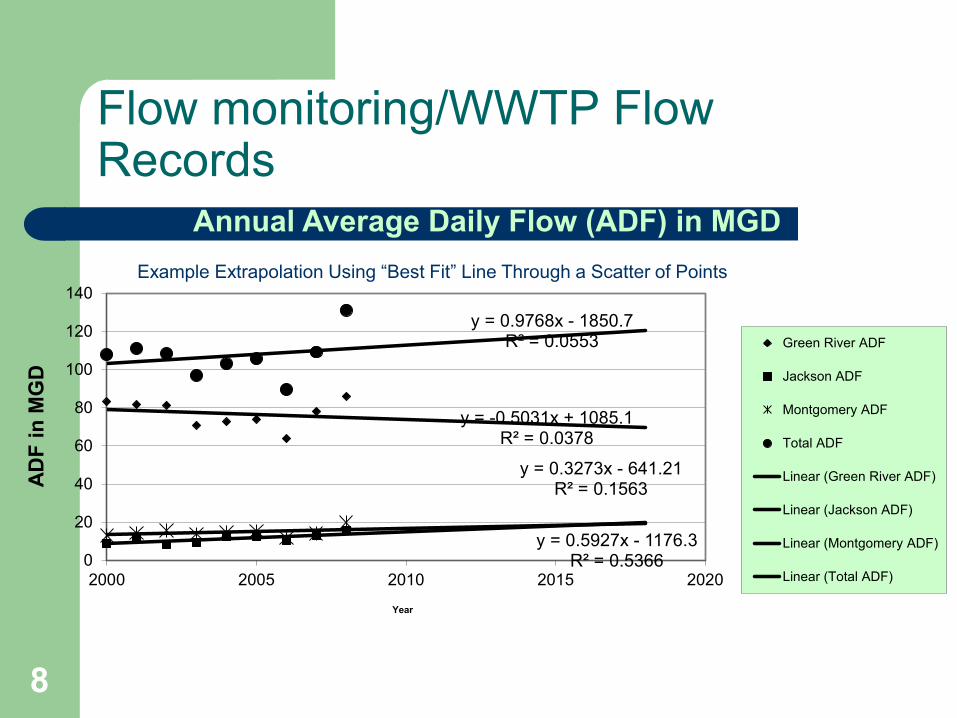
Flow monitoring/WWTP Flow Records

y = -0.5031x + 1085.1 R² = 0.0378

y = 0.5927x - 1176.3 R² = 0.5366

y = 0.3273x - 641.21 R² = 0.1563

y = 0.9768x - 1850.7 R² = 0.0553

0

20

40

60

80

100

120

140

2000 2005 2010 2015 2020

AD

F in

MG

D

Year

Annual Average Daily Flow (ADF) in MGD

Green River ADF

Jackson ADF

Montgomery ADF

Total ADF

Linear (Green River ADF)

Linear (Jackson ADF)

Linear (Montgomery ADF)

Linear (Total ADF)

Example Extrapolation Using “Best Fit” Line Through a Scatter of Points

9

Population Projections

Various mathematical extrapolation methods are used to obtain future population.

Historical water use or monitoring data provide per capita wastewater generation factors.

Base wastewater generation is the per capita rate multiplied by the population.

Infiltration/Inflow should be estimated and added. Peak flow must be estimated from historical diurnal

(24-hour) wastewater flow patterns.

10

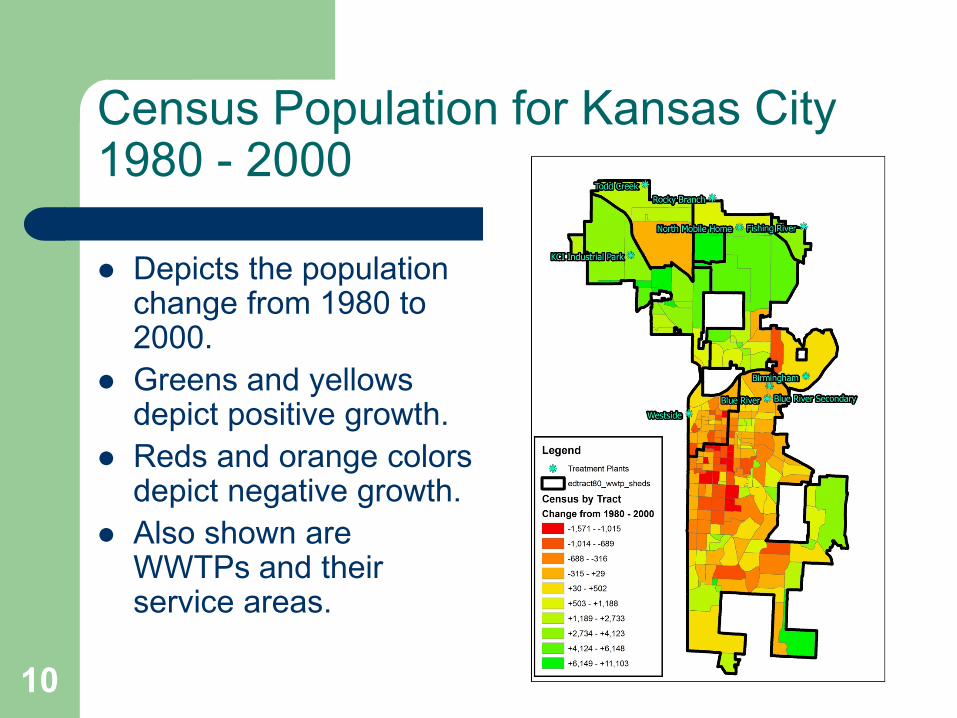
Census Population for Kansas City 1980 - 2000

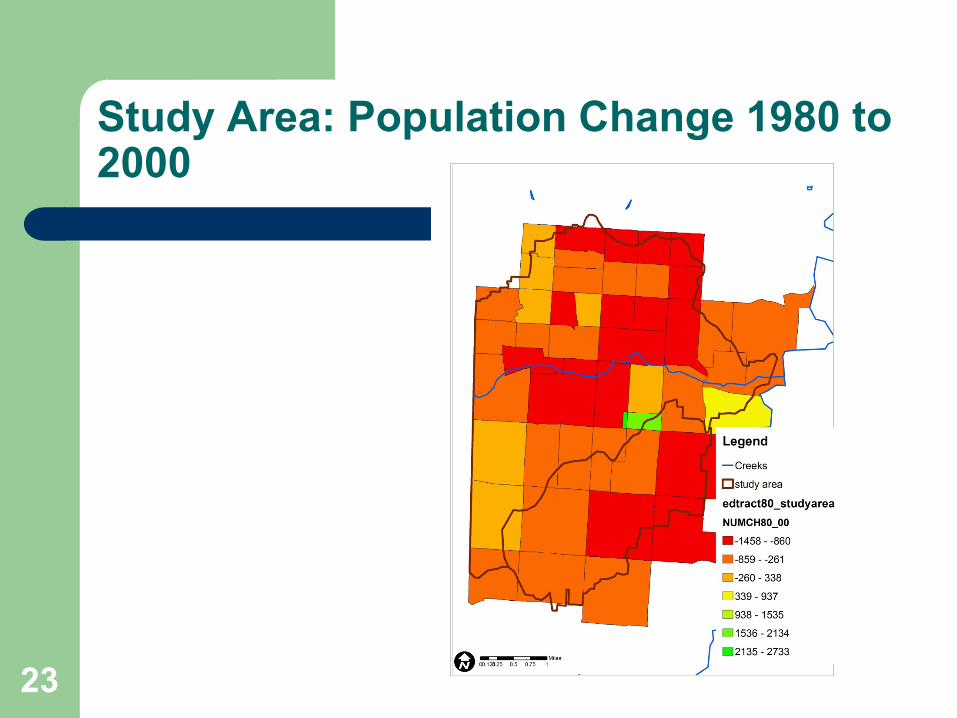
Depicts the population change from 1980 to 2000.

Greens and yellows depict positive growth.

Reds and orange colors depict negative growth.

Also shown are WWTPs and their service areas.

11

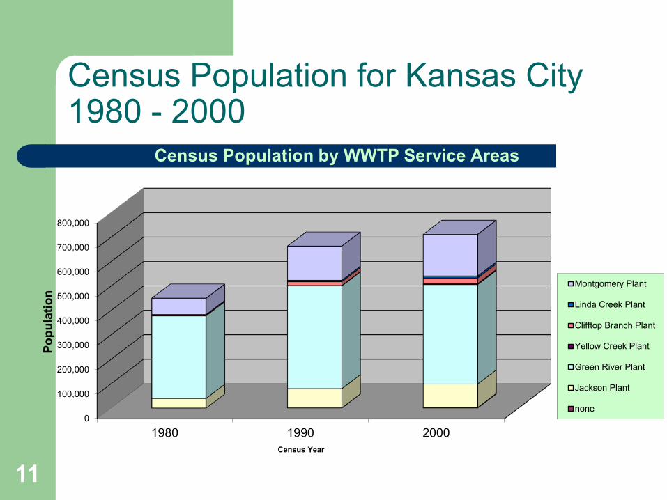
Census Population for Kansas City 1980 - 2000

0

100,000

200,000

300,000

400,000

500,000

600,000

700,000

800,000

1980 1990 2000

Popu

latio

n

Census Year

Census Population by WWTP Service Areas

Montgomery Plant

Linda Creek Plant

Clifftop Branch Plant

Yellow Creek Plant

Green River Plant

Jackson Plant

none

12

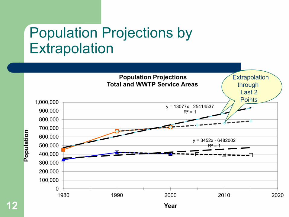
Population Projections by Extrapolation

y = 3452x - 6482002 R² = 1

y = 13077x - 25414537 R² = 1

0100,000200,000300,000400,000500,000600,000700,000800,000900,000

1,000,000

1980 1990 2000 2010 2020

Popu

latio

n

Year

Population Projections Total and WWTP Service Areas Best Fit

through 3

P

Extrapolation through

Last 2 Points

13

Wastewater Forecasts Based on Population Projections

Advantages: – Data is readily available for free. – Planning departments provide population

projections routinely. Disadvantages:

– Population projections do not accurately predict commercial and industrial wastewater generation.

14

Land use projections

Requires planning services to create future land use scenarios.

Historical water use or monitoring data provide per acre wastewater generation factors.

15

Wastewater Forecasts Based on Land Use Projections

Advantages: – Land use classes can account for any type of

generator and non-generator of wastewater. – Lends itself readily to digital GIS analysis.

Disadvantages: – Correlation of land area with wastewater

generation rates is not strong. – Predicting land use is more art than science. – Historical data is often hard to get.

16

Synchronize Data

Population, land use and wastewater generation rates are continuously changing.

As closely as possible, select billing data, land use and population from the same time period.

17

The Practice of Forecasting

18

Example Forecasting Using Actual Data

Demonstrate GIS techniques for forecasting wastewater using billing data, population and land use.

Derive unit rates of generation by exploiting the spatial relationships between billing data, population and land use.

19

Process Description

Identify the Study Area. Find the per capita water use. Multiply the projected population by the per

capita water use to estimate base flow. Use typical factors to account for

Infiltration/Inflow (I/I). Use peaking factors to find the typical peak

flow.

20

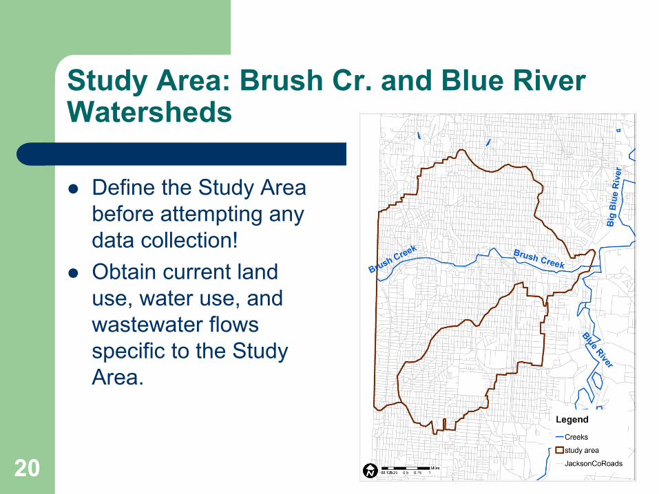
Study Area: Brush Cr. and Blue River Watersheds

Define the Study Area before attempting any data collection!

Obtain current land use, water use, and wastewater flows specific to the Study Area.

21

Data Collected

Population - Missouri Spatial Data Information Service (MSDIS) provided 1980, 1990, and 2000 Census data.

Land Use - Derived from City DMS Parcels GIS data. Annual and monthly wastewater Flows 2000 - 2008-

Provided by City staff. Water Meter Data – Obtained from the City.

22

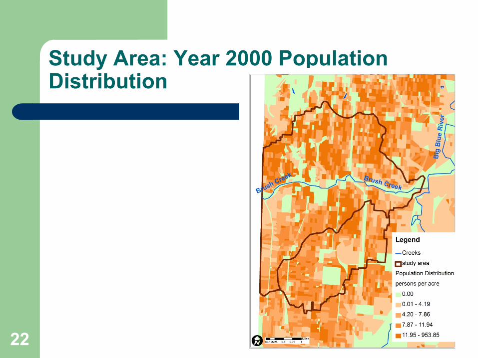
Study Area: Year 2000 Population Distribution

23

Study Area: Population Change 1980 to 2000

24

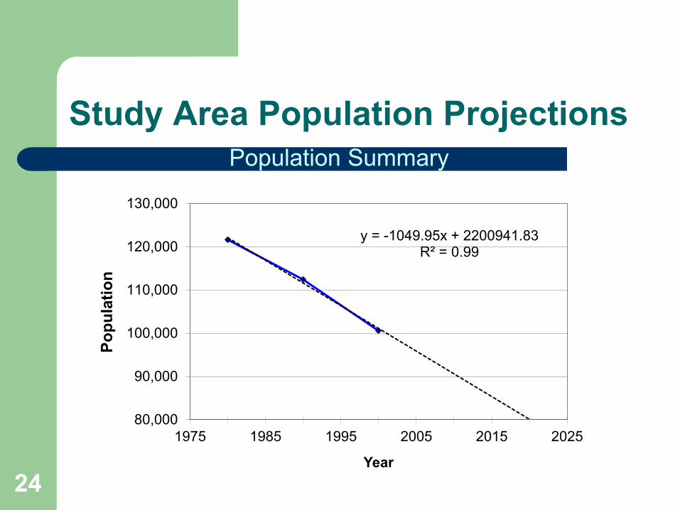
Study Area Population Projections

y = -1049.95x + 2200941.83 R² = 0.99

80,000

90,000

100,000

110,000

120,000

130,000

1975 1985 1995 2005 2015 2025

Popu

latio

n

Year

Population Summary

25

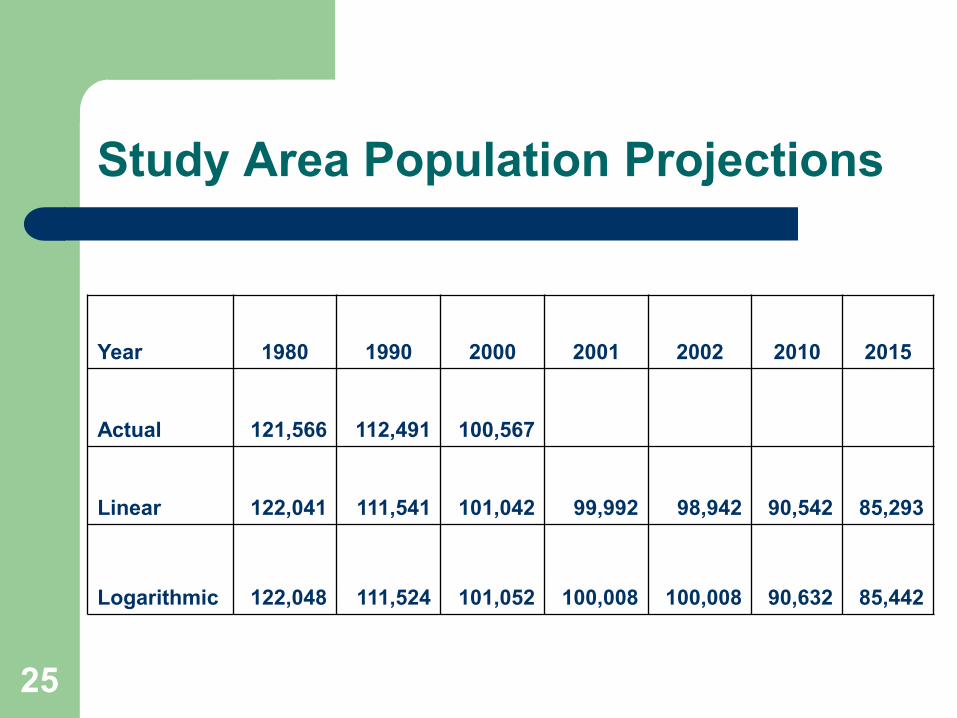
Study Area Population Projections

Year 1980 1990 2000 2001 2002 2010 2015

Actual 121,566 112,491 100,567

Linear 122,041 111,541 101,042 99,992 98,942 90,542 85,293

Logarithmic 122,048 111,524 101,052 100,008 100,008 90,632 85,442

26

City Water Use Data

Spreadsheet format exported from database Meter number Address of meter location Time period – November through January Metered water volume – 100 cubic feet units Use class: Commercial, Free water, Large

Commercial, Residential

27

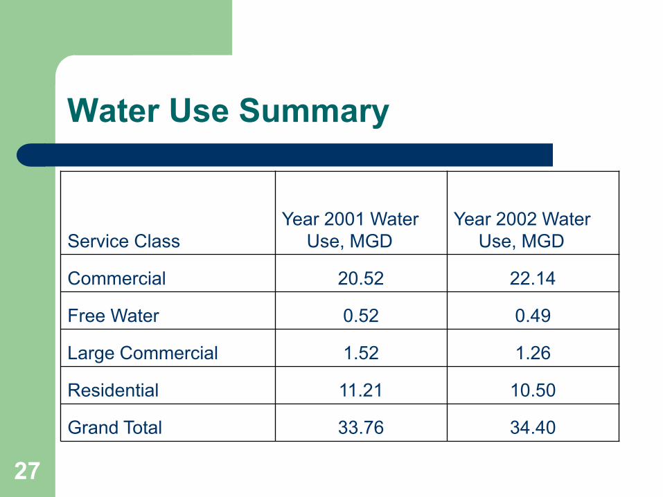
Water Use Summary

Service Class Year 2001 Water

Use, MGD Year 2002 Water

Use, MGD

Commercial 20.52 22.14

Free Water 0.52 0.49

Large Commercial 1.52 1.26

Residential 11.21 10.50

Grand Total 33.76 34.40

28

Forecasting Water Use Classes

Water is used by: – Residents. – Employees of commercial establishments. – Employees of factories and repair shops. – The City utilities

Each uses and disposes of water differently. Each has a different water use trend. We will assume that all these groups generally

follow the population trend.

29

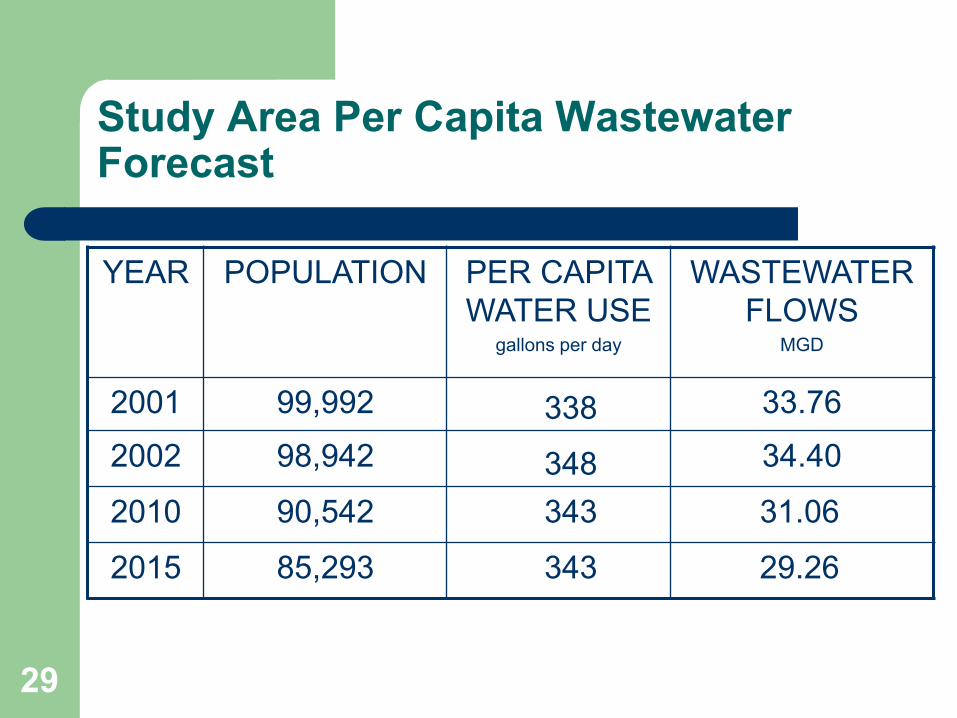
Study Area Per Capita Wastewater Forecast

YEAR POPULATION PER CAPITA WATER USE

gallons per day

WASTEWATER FLOWS

MGD

2001 99,992 33.76

2002 98,942 34.40

2010 90,542

2015 85,293

338

348 343

343

31.06

29.26

30

Accounting for I/I

Rigorous accounting for Infiltration/Inflow (I/I) requires flow monitoring studies, rainfall data collection and analysis.

Combined sewers behave more like storm sewers during wet weather.

Peak flows in combined sewer areas are limited by the capacity of the sanitary sewers.

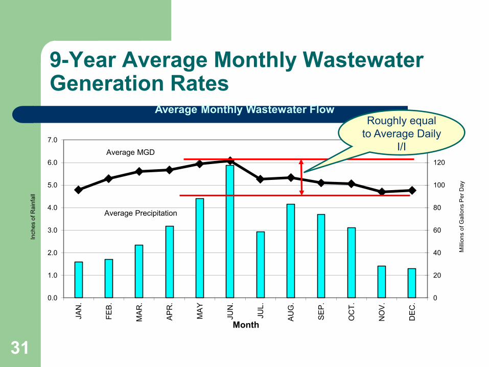
31

Average Precipitation

Average MGD

0

20

40

60

80

100

120

140

0.0

1.0

2.0

3.0

4.0

5.0

6.0

7.0

JAN

.

FEB

.

MA

R.

AP

R.

MA

Y

JUN

.

JUL.

AU

G.

SE

P.

OC

T.

NO

V.

DE

C.

Month

Average Monthly Wastewater Flow

Inch

es o

f Rai

nfal

l

Milli

ons

of G

allo

ns P

er D

ay

9-Year Average Monthly Wastewater Generation Rates

Roughly equal to Average Daily

I/I

32

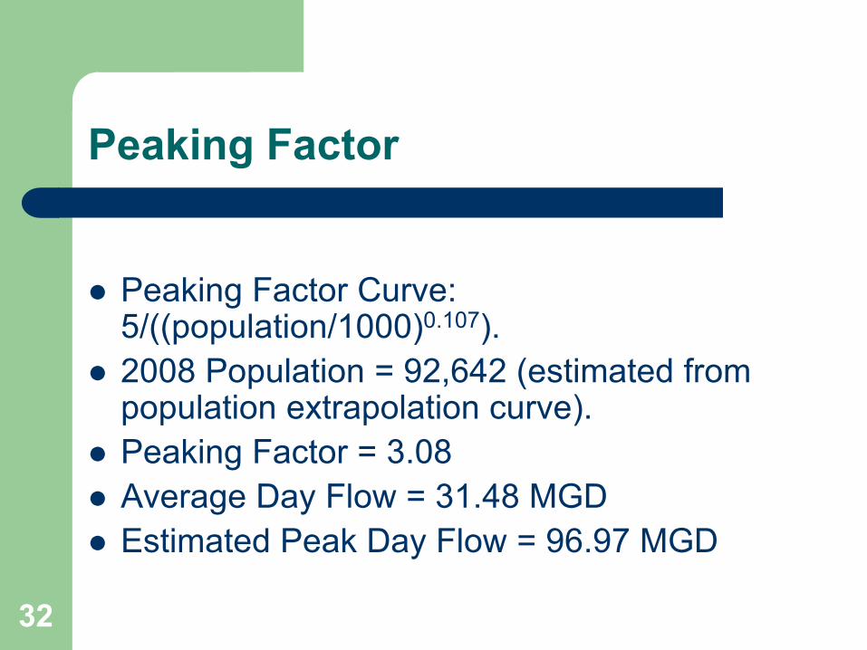
Peaking Factor

Peaking Factor Curve:

5/((population/1000)0.107). 2008 Population = 92,642 (estimated from

population extrapolation curve). Peaking Factor = 3.08 Average Day Flow = 31.48 MGD Estimated Peak Day Flow = 96.97 MGD

33

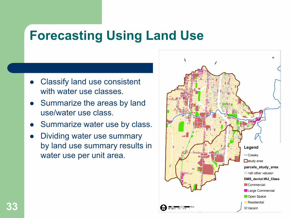
Forecasting Using Land Use

Classify land use consistent with water use classes.

Summarize the areas by land use/water use class.

Summarize water use by class. Dividing water use summary

by land use summary results in water use per unit area.

34

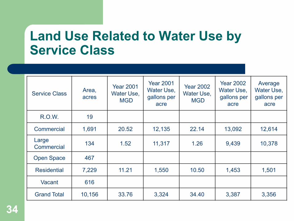
Land Use Related to Water Use by Service Class

Service Class Area, acres

Year 2001 Water Use,

MGD

Year 2001 Water Use, gallons per

acre

Year 2002 Water Use,

MGD

Year 2002 Water Use, gallons per

acre

Average Water Use, gallons per

acre

R.O.W. 19

Commercial 1,691 20.52 12,135 22.14 13,092 12,614

Large Commercial 134 1.52 11,317 1.26 9,439 10,378

Open Space 467

Residential 7,229 11.21 1,550 10.50 1,453 1,501

Vacant 616

Grand Total 10,156 33.76 3,324 34.40 3,387 3,356

35

A Teaching Moment

36

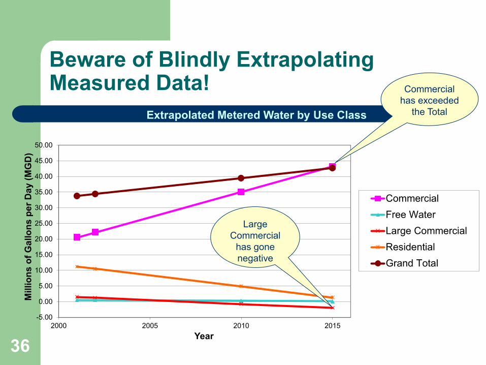
Beware of Blindly Extrapolating Measured Data!

-5.00

0.00

5.00

10.00

15.00

20.00

25.00

30.00

35.00

40.00

45.00

50.00

2000 2005 2010 2015

Mill

ions

of G

allo

ns p

er D

ay (M

GD

)

Year

Extrapolated Metered Water by Use Class

CommercialFree WaterLarge CommercialResidentialGrand Total

Commercial has exceeded

the Total

Large Commercial

has gone negative

37

Land Use Projection Assumptions

Loss of Residential Area is Proportional to Population Decrease – 79.2 acres per year.

Three-quarters of the Loss is Permanent – turns into Open Space or Vacant.

Quarter of the Loss becomes Commercial. Large Commercial is assumed constant.

38

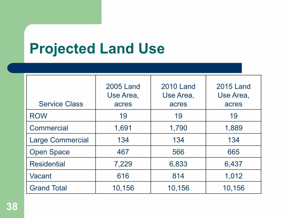
Projected Land Use

Service Class

2005 Land Use Area,

acres

2010 Land Use Area,

acres

2015 Land Use Area,

acres ROW 19 19 19 Commercial 1,691 1,790 1,889 Large Commercial 134 134 134 Open Space 467 566 665 Residential 7,229 6,833 6,437 Vacant 616 814 1,012 Grand Total 10,156 10,156 10,156

39

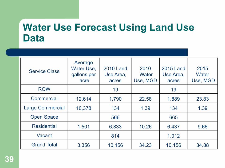
Water Use Forecast Using Land Use Data

Service Class

Average Water Use, gallons per

acre

2010 Land Use Area,

acres

2010 Water

Use, MGD

2015 Land Use Area,

acres

2015 Water

Use, MGD

ROW 19 19

Commercial 12,614 1,790 22.58 1,889 23.83

Large Commercial 10,378 134 1.39 134 1.39

Open Space 566 665

Residential 1,501 6,833 10.26 6,437 9.66

Vacant 814 1,012

Grand Total 3,356 10,156 34.23 10,156 34.88

40

Converting Water Use to Wastewater Flows

Not all Metered Water is delivered to the sewer. – Irrigation. – Exterior washing. – Sold as part of product.

The most rigorous forecasts account for “return water” and analyze flows for infiltration and inflow.

Losses often balance with infiltration and inflow in residential and commercial dominated areas.

This demonstration assumes Water Use = Wastewater Flow.

41

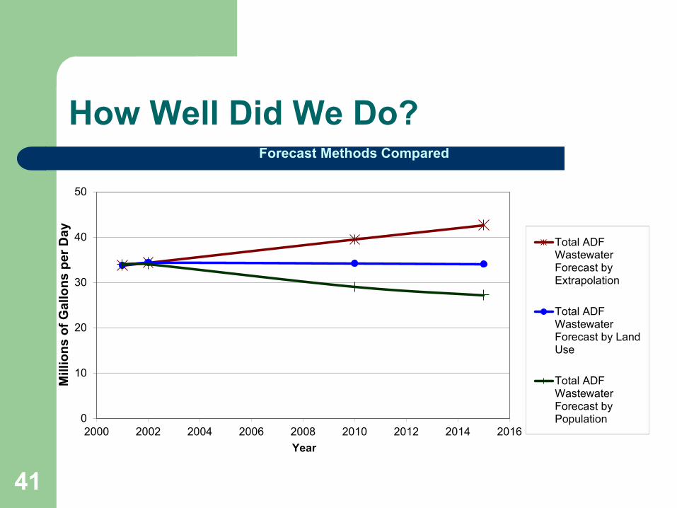
How Well Did We Do?

0

10

20

30

40

50

2000 2002 2004 2006 2008 2010 2012 2014 2016

Mill

ions

of G

allo

ns p

er D

ay

Year

Forecast Methods Compared

Total ADFWastewaterForecast byExtrapolation

Total ADFWastewaterForecast by LandUse

Total ADFWastewaterForecast byPopulation

42

Why the Differences?

The Extrapolation assumed that water usage for two years was sufficient to establish the overall trend.

The Land Use method respected differing trends between land use classes – some were upward, others downward.

The Population method assumed that all growth was proportional to the population trend, which was downward.

43

Process Review

Use GIS to establish the relationships among water use, land use, and population.

Summarize flows by population distribution and/or land use areas.

Calculate unit flow rates per person and/or per unit land area.

Extrapolate population and/or land areas into the future.

Multiply unit flow rates by the extrapolated future population and/or land areas.

44

Conclusion

Many methods exist for forecasting wastewater flows.

Each method has advantages and disadvantages.

Select the method best fitted for the purpose and the location.