Embed Size (px)
Citation preview
Approval Sheet
Title of Thesis: Performance Analysis of the IEEE 802.11 Wireless LAN Standard
Name of Candidate: Craig Sweet Master of Science, 1999
Thesis and Abstract Approved: _______________________________________
Dr. Deepinder Sidhu Professor Department of Computer Science and Electrical Engineering
Date Approved: _____________________________________________________

Curriculum Vitae
Name: Craig Sweet
Permanent Address: 2-I Quiet Stream Ct. Timonium, MD 21093
Degree and date to be conferred: Master of Science, 1999
Date of Birth: August 15, 1972
Place of Birth: Baltimore, MD
Education:
High School Diploma June 1990 Perry Hall High School, Perry Hall MD
A.A. June 1992 Essex Community College, General Studies
B.S. Dec. 1994 UMBC, Computer Science
M.S. May 1999 UMBC, Computer Science
Major: Computer Science
Professional Position: President - Microcomm Consulting, Inc.
PO Box 117
Kingsville, MD 21087

Abstract
Title of Thesis: Performance Analysis of the IEEE 802.11 Wireless LAN Standard
Thesis directed by: Dr. Deepinder Sidhu Professor Department of Computer Science and Electrical Engineering
IEEE 802.11 is a relatively new standard for communication in a wireless LAN. Its need
arose from the many differences between traditional wired and wireless LANs and the
increased need for interoperability among different vendors. The Medium Access
Control (MAC) portion of 802.11 uses collision avoidance since it cannot reliably detect
collisions, a major difference from Ethernet. As a result, the protocol is less efficient
than its wired counterpart. To date, detailed performance measures for this CSMA/CA
protocol are not known. In this thesis, we implemented a Discrete-Event Simulation to
model the Distributed Coordination Function (DCF) of the MAC sublayer. We model an
ideal LAN and describe the best case performance. The results of this work show how
the protocol performance is affected by fluctuations in the properties of the system. This
information is useful in determining the maximum performance that can be expected.

Performance Analysis of the IEEE 802.11 Wireless LAN
Standard
by Craig Sweet
Thesis Submitted to the Faculty of the Graduate School of the University of Maryland in partial fulfillment
of the requirements for the degree of Master of Science
1999


ii
To my Parents
Joseph and Elizabeth Carol Sweet

iii
Acknowledgements
I would like to express my sincere appreciation to my research advisor Dr. Deepinder
Sidhu for his guidance as well as patience during the course of preparing this thesis.
Additionally, I would like to thank Dr. Chein-I Chang, and Dr. Fow-Sen Choa for their
participation on my thesis committee.
Finally, I would like to thank the members of the Maryland Center for
Telecommunications Research (MCTR) for their support and guidance through this
research project.
iv
Table of Contents
1 Introduction..........................................................................................................................................1
2 The IEEE 802.11 Wireless LAN Standard .................................................................................3
2.1 Attributes of Wireless LAN's ............................................................................................................4 2.2 Physical Medium Specification.........................................................................................................5 2.3 Distributed Coordination Function ...................................................................................................6 2.4 Point Coordination Function...........................................................................................................11
3 Modeling & Simulation ..................................................................................................................13
3.1 Assumptions....................................................................................................................................13 3.2 Description of Simulation Model....................................................................................................14 3.3 Offered Load Computation .............................................................................................................15
4 Performance Analysis .....................................................................................................................16
4.1 Experiment 1: Variable Load ..........................................................................................................16 4.2 Experiment 2: Variable Stations .....................................................................................................18 4.3 Experiment 3: Variable Fragmentation ...........................................................................................21 4.4 Experiment 4: Variable Propagation Delay.....................................................................................23
5 Conclusion..........................................................................................................................................27
6 Future Work .......................................................................................................................................28
7. Bibliography ......................................................................................................................................29

v
List of Figures
Figure 2.1 : Inter-Frame Space and Backoff Window Relationship...........................................7
Figure 2.2 : Backoff Procedure Example ...........................................................................................8
Figure 2.3 : RTS Exchange Example.................................................................................................10
Figure 4.1 : Throughput vs. Offered Load at 1 Mbit/s .................................................................17
Figure 4.2 : Throughput vs. Number of Stations............................................................................19
Figure 4.3 : Throughput vs. Fragmentation Threshold.................................................................21
Figure 4.4 : Throughput vs. Propagation Delay (1 Mbit/s) .........................................................24
Figure 4.5 : Throughput vs. Propagation Delay (2 Mbit/s) .........................................................25
Figure 4.6 : Throughput vs. Propagation Delay (10 Mbit/s).......................................................26

vi
List of Tables
Table 4.1 : Simulation Results at 200% Load for Variable Packet Sizes................................18
Table 4.2 : Simulation Results at 100% Load for Variable Number of Stations ..................20
Table 4.3 : Simulation Results at 200% Load for Variable Fragmentation Threshold .......23

1
Chapter 1 Introduction
Over the last several years, we have witnessed widespread deployment of Wireless LANs
in virtually every industry. Increasingly, organizations are finding that wireless LANs
are an indispensable addition to their network infrastructure since they provide mobility,
and coverage of locations that are difficult to reach by wires. Manufacturing plants, stock
exchange floors, warehouses, historical buildings, and small offices are examples of
environments that are sometimes difficult to cable. Additionally, barriers such as high
prices and difficult licensing requirements have been overcome.
Until recently, there has been no agreed upon standard by which wireless stations
communicate. This lack of standardization usually results in decreased interoperability
since each vendor’s proprietary systems cannot communicate with one another. The
Industry for Electrical and Electronics Engineers (IEEE) has been working with leaders
from industry to develop a standard to which wireless stations from different vendors can
conform. In 1997, the IEEE finally ratified their standard 802.11, the Physical and MAC
specification for Wireless LANs [IEE97].
Since traditional Ethernet has been in existence for quite some time, much research has
been done studying its attributes under various conditions [BUX81, GON83, and
GON87]. A detailed study of the Carrier Sense Multiple Access with Collision Detection
scheme used in Ethernet can be found in [TOB80].

2
Since 802.11 is a recent development, not much is known about how the protocol
performs. The goal of this research is to better understand how this new protocol
performs under a variety of conditions.
We begin in chapter 2 by describing the features of the 802.11 Medium Access Control
(MAC) sublayer protocol. This includes a detailed description of the Distributed
Coordination function (DCF) and the Point Coordination Function (PCF). As with any
performance measure, a detailed description of the modeling techniques is necessary to
compare results from different experiments. Chapter 3 describes the computational
model used in this work and explains the assumptions and other pertinent information.
Chapter 4 is the heart of the thesis and describes the experiments that were run and
analyzes the results. It is here that we see the true performance metrics for the protocol
under ideal conditions. Chapter 5 adds some concluding remarks and chapter 6 suggests
some future work that could be done to extend this analysis.

3
Chapter 2 The IEEE 802.11 Wireless LAN Standard
Stations participating in a wireless LAN have fundamental differences from their
traditional wired counterparts. Despite these differences, 802.11 is required to appear to
higher layers (LLC) as a traditional 802 LAN. All issues concerning these differences
must be handled within the MAC layer. This chapter presents the concepts and
terminology used within an 802.11 implementation. For a more detailed description of
the 802.11 specification the reader is referred to [IEE97].
One major difference is the wireless station’s lack of a fixed location. In a wireless LAN,
a station is not assumed to be fixed to a given location. Users are grouped into two
classifications, mobile and portable. Portable users are those that move around while
disconnected from the network but are only connected while at a fixed location. Mobile
users are those users that remain connected to the LAN while they move. IEEE 802.11 is
required to handle both types of stations.
Due to differences in the physical medium, wireless LANs also employ a much different
physical layer. The physical medium has no fixed observable boundaries outside of
which the station cannot communicate. Outside signals are also a constant threat. The
end result is that the medium is considerably less reliable. Also, the assumption of full
connectivity will not always hold true. A station may come into or go out of contact with
other stations without leaving the coverage area of the physical layer.
4
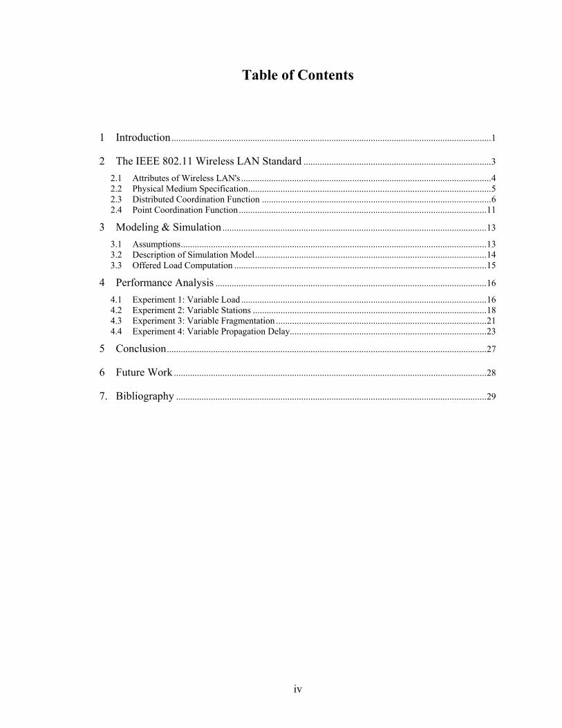
2.1 Attributes of Wireless LAN's
Wireless LANs must adhere to the many of the same rules as traditional wired LANs,
including full connectivity to stations, the ability to broadcast, high capacity, etc. In
addition, wireless LANs have some special requirements unique to their form of
communication [STA97]. A few of these follow:
• Throughput - Due to the decreased bandwidth of radio and IR channels, the Medium
Access Control (MAC) protocol should make as efficient use of this available
bandwidth as possible.
• Backbone Connectivity - In most cases, wireless LANs connect to some sort of
internal (wired) network. Therefore, facilities must be provided to make this
connection. This is usually one station that also serves as the Access Point (AP) to the
wired LAN for all stations
• Power Considerations - Often times, wireless stations are small battery powered
units. Algorithms that require the station to constantly check the medium or perform
other tasks frequently may be inappropriate.
• Roaming - Wireless stations should be able to move freely about their service area.

5
• Dynamic - The addition, deletion, or relocation of wireless stations should not affect
other users
• Licensing - In order to gain widespread popularity, it is preferred that FCC licenses
not be required to operate wireless LAN's.
2.2 Physical Medium Specification
As mentioned previously, the wireless physical medium is considerably different than
that of traditional wired LANs. Well-defined coverage areas do not exist. The
propagation characteristics between stations are dynamic and unpredictable and this
drastically influenced the design of the MAC layer. The Physical layer of the IEEE
802.11 specification provides for stations communicating via one of three methods:
• Infrared (IR) - Transmits the signal using near-visible light in the 850-nanometer to
950-nanometer range. This is similar to the spectral range of infrared remote
controls, but unlike these devices, wireless LAN IR transmitters are not directed.
• Direct Sequence Spread Spectrum (DSSS) - Transmits the signal simultaneously
over a broad range of frequencies.

6
• Frequency Hopping Spread Spectrum (FHSS) - Transmits the signal across a
group of frequency channels by hopping from frequency to frequency after a given
dwell-time. This form of Spread Spectrum is more immune to jamming.
2.3 Distributed Coordination Function
IEEE 802.11 uses a system known as Carrier Sense Multiple Access with Collision
Avoidance (CSMA/CA) as its Distributed Coordination Function (DCF). All stations
participating in the network use the same CSMA/CA system to coordinate access to the
shared communication medium.
A station that wishes to transmit must first listen to the medium to detect if another
station is using it. If so it must defer until the end of that transmission. If the medium is
free then that station may proceed.
Two mechanisms are included to provide two separate carrier sense mechanisms. The
traditional physical carrier sense mechanism is provided by the physical layer and is
based upon the characteristics of the medium. In addition, the Medium Access Control
(MAC) layer also provides a virtual mechanism to work in conjunction with the physical
one. This virtual mechanism is referred to as the Network Allocation Vector (NAV).
The NAV is a way of telling other stations the expected traffic of the transmitting station.

7
A station’s medium is considered busy if either its virtual or physical carrier sense
mechanisms indicate busy.
Before a station can transmit a frame, it must wait for the medium to have been free for
some minimum amount of time. This amount of time is called the Inter-frame Space
(IFS). This presents an opportunity to establish a priority mechanism for access to the
shared medium. Depending upon the state of the sending station, one of four Inter-Frame
spaces is selected. In ascending order, these spaces are the Short IFS (SIFS), PCF IFS
(PIFS), DCF IFS (DIFS), and Extended IFS (EIFS). The MAC protocol defines instances
where each IFS is used to support a given transmission priority.
A station wishing to transmit either a data or management frame shall first wait until its
carrier sense mechanism indicates a free medium. Then, a DCF Inter-Frame Space will
be observed. After this, the station shall then wait an additional random amount of time
before transmitting. This time period is known as the backoff interval. The purpose of
this additional deferral is to minimize collisions between stations that may be waiting to
transmit after the same event. This operation is called the Backoff Procedure and is
shown in figure 2.1 [IEE97]
DIFS
Busy Medium
DIFS
SIFS
PIFS
Next Frame Backoff-Window
Contention Window
Defer Access Select slot and Decrement Backoff as long as medium is idle
Immediate access when medium is free >= DIFS
Slot
Fig. 2.1. Inter-Frame Space and Backoff Window Relationship

8
Before a station can transmit a frame it must perform this backoff procedure. The station
first waits for a DIFS time upon noticing that the medium is free. If, after this time gap,
the medium is still free the station computes an additional random amount of time to wait
called the Backoff Timer. The station will wait either until this time has elapsed or until
the medium becomes busy, whichever comes first. If the medium is still free after the
random time period has elapsed, the station begins transmitting its message. If the
medium becomes busy at some point while the station is performing its backoff
procedure, it will temporarily suspend the backoff procedure. In this case, the station
must wait until the medium is free again, perform a DIFS again, and continue where it
left off in the backoff procedure. Note that in this case it is not necessary to re-compute a
new Backoff Timer. An example of the backoff procedure is shown in figure 2.2
[IEE97].
Frame
Frame
Frame
Frame
Frame
CWindow
CWindow
CWindow
Backoff
CWindow
Defer
Defer
Defer
Defer
DIFS CWindow = Contention Window
= Remaining Backoff = Backoff
Fig. 2.2. Backoff Procedure Example

9
Upon the reception of directed (not broadcast or multicast) frames with a valid CRC, the
receiving station will respond back to the sending station an indication of successful
reception, generally an acknowledgement (ACK). This process is known as positive
acknowledgement. A lack of reception of this acknowledgement indicates to the sending
station that an error has occurred. Of course, it is possible that the frame may have been
successfully delivered and the acknowledgement was unsuccessful. This is
indistinguishable from the case where the original frame itself is lost. As a result, it is
possible for a destination station to receive more than one copy of a frame. It is therefore
the responsibility of the destination to filter out all duplicate frames.
With the exception of positive acknowledgements, the mechanism described so far is
very similar to that of traditional Ethernet (802.3). Additionally, 802.11 provides a
request-to-send procedure which is intended to reduce collisions. Stations gain access to
the medium in the same way but instead of sending its first data frame, the station first
transmits a small Request-to-Send (RTS) frame. The destination replies with a Clear-to-
Send (CTS) frame. The NAV setting within both the RTS and CTS frames tell other
stations how long the transmission is expected to be. By seeing these frames, other
stations effectively turn on their virtual carrier sense mechanism for that period of time.
While there may be high contention for the medium while the RTS frame is attempted,
the remainder of the transmission should be relatively contention-free. This improves the
performance of the protocol because all collisions occur on the very small RTS frames
and not on the substantially larger data frames. The use of the RTS/CTS mechanism is

10
not mandatory and is activated via a Management Information Base (MIB) variable.
Figure 2.3 [IEE97] shows an example of an RTS exchange.
When beginning a transmission that will include more than one fragment, known as a
fragment burst, the rules change slightly. Initially it appears identical to a single
fragment transmission. The backoff and carrier sense procedures are the same. The
difference lies in the IFS used between fragments. Only a SIFS is required between
fragments during a fragment burst. The reason for this is to give the sender the highest
priority when transmitting a fragment burst. Consider two examples where this may
come into play. In the first example a station with no knowledge of the NAV, perhaps
having recently joined the network, must try to wait a DIFS before transmitting. After a
shorter SIFS the original station takes over the medium with its next fragment and this
other station, upon noticing a busy medium, must defer. As a second example a point
coordinator, described in the next section, which must wait a PIFS wants to take control
of the medium. Since the Point Coordinator observes a shorter IFS than other stations’
NAV (RTS)
Contention Window
Defer Access Backoff After Defer
DIFS
SIFS
DataRTS DIFS
SIFS CTS
SIFS
Sender
Receiver
Other
ACK
NAV (CTS)
Fig. 2.3. RTS Exchange Example

11
and a longer one than the station transmitting a fragment burst, it (the point coordinator)
must defer until after the fragment burst.
When transmitting broadcast or multicast frames, only the basic transfer mechanism is
used. No RTS/CTS mechanism is used regardless of the size of the frame. Additionally,
no receiving station will ever respond with an ACK to a broadcast or multicast frame.
2.4 Point Coordination Function
In addition to the DCF, an optional Point Coordination Function (PCF) is also provided.
The basic principles of the PCF work on top of the mechanisms already provided by the
DCF. Thus, all stations inherently coexist with other stations utilizing the PCF function,
whether or not they themselves utilize this optional function.
Under PCF, the Access Point (AP) to the wired network optionally chooses to become a
Point Coordinator (PC). In fact, only the AP can make the decision to become the PC.
The PC uses Beacon Management Frames to gain control of the medium by setting the
NAV in all stations to busy. Remember that the PC, using a PIFS, has a higher priority
than all other stations except one involved in a fragment burst. Since all stations must
observe the DCF access rules, they cannot transmit with a NAV value greater than 0.
This in effect gives control of the medium to the PC by turning off all other stations’
ability to transmit for a given amount of time.

12
Once the PC has taken control of the medium it can then poll each station, one at a time,
giving it an opportunity to transmit free of contention. The rules against transmitting
when your NAV indicates a busy medium are ignored only when responding to a poll
from a PC. The PC can therefore take control of the medium and allow each station to
transmit any data it may have in turn.
The period of time that a PC has control of the medium is called a Contention Free Period
(CFP). The PCF access rules state that a CFP must alternate with a Contention Period
(CP), where the DCF controls frame transfers. The AP can only schedule CFPs in
alternation with CPs. This is to allow fairness to stations that do not observe the PCF
access procedure.

13
Chapter 3 Modeling & Simulation
In our experiments, our goal was to explore the efficiency of the MAC protocol under
ideal conditions. While many of these conditions may be unrealistic, the end result is
useful in telling us the highest performance that can be expected from the protocol. This
section describes some of the assumptions and limitations assumed in our system. Also,
the simulation model and computation variables are described.
3.1 Assumptions
All stations are assumed to be using a Direct Sequence Spread Spectrum (DSSS) radio.
The operation of Frequency Hopping Spread Spectrum (FHSS) and Infrared (IR) radios
had too much of an impact on a given transmission to study the aspects of the protocol
itself. Additionally, it is assumed that there are no power considerations for either the
radios or the wireless stations that could interfere with the operation of the protocol.
All stations are assumed to be transmitting using the same data rate. In this analysis,
speeds of 1, 2, and 10 Megabits per Second (Mbit/s) are used. While only 1 and 2 Mbit/s
are listed in the 802.11 specification, 10 Mbit/s was included since current research is
aimed at providing radios that work at this and higher speeds.

14
A significant aspect of any transmission protocol is how it handles transmission errors.
In order to focus on the best case performance of the MAC protocol, we assumed error-
free channels. Additionally, all stations have unobstructed access to all other stations and
thus can hear all transmissions.
To minimize complexity, we chose to model our wireless LAN as an ad-hoc network,
also known as an Independent Basic Service Set (IBSS). This is the simplest type of
wireless LAN defined in the standard. There is no Access Point and therefore no tie to a
wired LAN.
Finally, we decided to only model the DCF portion of the protocol. The DCF forms the
heart of the MAC protocol. The PCF has been omitted in this simulation, as it is an
optional portion of the MAC protocol that works on top of the DCF and can significantly
alter its results.
3.2 Description of Simulation Model
To perform this analysis, we constructed a discrete-event simulation of the MAC portion
of the IEEE 802.11 protocol. A complete description of simulation techniques can be
found in [BAN84]. This simulation is software that has been tested to conform to all
aspects of the DCF portion of the protocol. To eliminate any initialization biases, we
allowed the simulation to run for various amounts of time before collecting data. After

15
initialization, we allowed the system to run for another 60 seconds. Our tests showed no
significant differences in runs longer than 60 seconds.
A MAC Service Data Unit (MSDU) is the basic unit delivered between two compatible
MAC sub-layers. For all experiments, each station is assumed to have a one MSDU
buffer. For uniformity all MSDUs transmitted are of equal size. Initially, each station is
given one MSDU to transmit. Upon completing the transmission attempt, another MSDU
is assigned for transmission after some exponentially distributed inter-arrival time. In
this manner, changing the mean inter-arrival time between MSDUs can be used to alter
system load.
3.3 Offered Load Computation
Upon transmitting a message, the station generates the next message with an inter-arrival
time exponentially distributed with mean θ. Additionally, each station is sending the
same size packets, in bytes P, for the duration of a run. The offered load of station i, Gi,
is defined as in [GON87] to be the throughput of station i if the network had infinite
capacity, i.e.,
Gi = Tp / θI
where Tp = P/C and C is the transmission speed in Mbit/s. The total offered load can thus
be computed to be:
∑=
N
iiG
1

16
Chapter 4 Performance Analysis
In this analysis, we performed four experiments measuring various aspects of the MAC
protocol. Each of these experiments was conducted at several transmission speeds. 1 and
2 Mbit/s were selected because they are explicitly supported in the specification. 10
Mbit/s was selected to provide a comparison at traditional LAN speeds. The results of
these experiments are the topic of this section. Current research is aimed at providing
802.11 operation at 10 and 20 Mbit/s.
4.1 Experiment 1: Variable Load
In our first experiment we wanted to see what effect the total load on the system played
on performance. This experiment is similar to one found in [GON87]. Figure 4.1 shows
the variation of total throughput with total offered load G for various message sizes P at 1
Mbit/s. In this experiment, the fragmentation threshold has been set to 2346 bytes and
the RTS threshold has been set to 3000 bytes.
We can see that with an offered load of about 80% or less virtually no collisions occur
and throughput and load are approximately equal. Once the system load increases
beyond 90-100% we see the impact of collisions. As can be expected, greater throughput
is achieved via a greater packet size. Due to the overhead present in the protocol,
acceptable throughput was not seen with packet sizes below 2000 bytes.

17
Packet sizes above and below the fragmentation threshold did not yield much difference.
Even then, it all but disappeared with loads in excess of 200%. While increasing the
number of packets per message produces more overhead, it also reduces the collision
probability.
In this example, the RTS threshold played a crucial role in the performance of the
protocol. The throughput peaked out at approx. 80% for all packet sizes below 3000
bytes. For packet sizes above the RTS threshold, noticeable performance gains were seen
and throughput peaked at 96%.
Fig. 4.1. Throughput vs. Offered Load at 1 Mbit/s, 32 stations, Parameter, P.
0
20
40
60
80
100
10 20 40 100 200 400 800 1000
Total Offered Load, %
Net
Thr
ough
put,
%
P=2347
P=4500
P=2800
P=3200
P=512
P=128

18
As explained earlier, the RTS threshold acts as a medium reservation mechanism.
Collisions, and subsequent retransmissions, can occur on the smaller RTS frames but not
normally on the longer data frames. The result is a better utilization of the bandwidth.
Our results were similar for transmission speeds of 2 and 10 Mbit/s. Table 4.1
summarizes some of these results. What we saw was that as the transmission speed
increased, the throughput dropped. This can be attributed to the fact that the inter-frame
spaces are independent of transmission speed. At higher speeds, since it takes less time
to send the same packet, an IFS of 50 µs has more of an impact than at lower speeds.
Table 4.1 Simulation Results at 200% Offered Load for Various
Packet Sizes and Transmission Speeds
Mbit/s
Packet Size
Throughput %
1
4500 2800 2347
96.61 76.54 71.52
2
4500 2800 2347
96.11 76.07 73.08
10
4500 2800 2347
91.80 73.17 68.87
4.2 Experiment 2: Variable Stations
In our second experiment, our goal was to determine how many stations would overload
a wireless network. Certainly the performance characteristics for 10 stations would be

19
different than for 20 stations, all contending for access to the medium. Figure 4.2 shows
the effect on throughput with an increasing number of stations and a constant Offered
Load of 100%.
Results are shown both with and without the RTS mechanism implemented. For all runs,
the message size was set to 3000 bytes and the fragmentation threshold was set to 2346
bytes.
Without RTS enabled, we can see that the maximum throughput reached was approx.
82% with 16 participating stations. In fact, with few stations (below 16), we see that
there is not much difference in performance with and without RTS enabled.
As more stations are added to the simulation the probability that two or more stations will
calculate the same backoff window is increased. Thus, the chance for collision increases.
Fig. 4.2. Throughput vs. Number of stations with packet size above and below RTS Threshold (1 Mbit/s)
0
10
20
30
40
50
60
70
80
90
100
2 4 8 16 32 64 128 256 512 1024
Number of Stations
Net
Thr
ough
put,
%
No RTS RTS

20
This can be seen by the large differences between the RTS and No-RTS runs with higher
station counts, above 64.
Since IEEE 802.11 uses CSMA/CA, collisions are expensive. The transmitting station
must continue to transmit the entire message and wait a minimum amount of time before
determining that the transmission was in error. With RTS enabled, the collisions occur
on smaller RTS frames, allowing for a quicker turn-around time. We can see that with
RTS enabled, the system stabilized to approx. 92% or higher with 128 or more stations.
As in the previous experiment, we saw similar results in our 2 and 10 Mbit/s experiments.
As the speed of the medium increased there was still the same pattern between RTS and
No RTS results. We can see that higher transmission speeds yielded lower average
throughput results. Table 4.2 summarizes some of the results from these experiments
with and without RTS enabled.
Table 4.2 Simulation Results at 100% Offered Load with Variable
Number of Stations
Mbit/s
# of
Stations
Throughput with RTS
Throughput without RTS
16 82.59 81.93 128 92.38 76.22
1
1024 94.81 46.13 16 82.83 82.98 128 93.04 73.28
2
1024 94.07 53.91 16 80.34 78.01 128 88.6 70.04
10
1024 89.95 57.84

21
4.3 Experiment 3: Variable Fragmentation
In our third experiment, our goal was to determine what effect the fragment size played
on system performance. The simulation was run with 32 stations at 200% load with
varying fragmentation thresholds. Each message sent was 3000 bytes long. Therefore,
the fragmentation threshold merely determined how many fragments the 3000 byte
messages were broken up into.
Intuitively, advantages can be gained by both increasing and decreasing the
fragmentation threshold. Smaller thresholds limit the loss of performance due to
retransmissions but come with an increase in overhead. This is important because we
have already shown that the 802.11 protocol has considerable overhead. On the other
hand large fragmentation thresholds, while limiting the overhead, become expensive in
the event of a collision.
Fig. 4.3 Throughput vs. Fragmentation Threshold with packet size above and below RTS Threshold (1 Mbit/s)
60
70
80
90
100
250 500 750 1000 1250 1500 1750 2000 2346 3000
Fragmentation Threshold
Net
Thr
ough
put,
%
No RTS RTS

22
Figure 4.3 shows the results of this experiment run at 1 Mbit/s. As predicted, the RTS
mechanism does a great deal to improve the performance of this aspect of the protocol.
The reason can be attributed to the reduction in collisions that it provides. At smaller
thresholds, there is little difference between the RTS and No RTS figures. There is
nearly a balance between three factors: the overhead provided by the RTS mechanism,
the smaller fragment sizes that are retransmitted in the event of a collision, and the
overhead provided by multiple smaller fragments.
It is not until the fragmentation threshold increases that we see the largest variation in
performance. As was expected, with larger fragments comes a decrease in performance.
Each collision requires retransmission of a much larger fragment. Since 802.11 does not
have a collision detection mechanism the entire fragment must be transmitted before
success or failure of that fragment can be determined.
This experiment has also shown that, in this specific case, little improvement can be seen
with fragments above 1000 bytes when the RTS mechanism is used. While this may be
true in this experiment, note that we are assuming that all fragments are transmitted error-
free. This assumption will certainly not hold in a real-world case. In fact, performance
may decrease as the bit-error rate increases. The probability of each fragment being
successfully delivered will decrease as the fragment size increases and results will most
certainly differ.

23
The results for 1, 2, and 10 Mbit/s experiments are summarized in Table 4.3. We can see
that the same pattern is exhibited regardless of the transmission speed. As we have seen
in the previous experiments, the constant inter-frame space times effectively reduce the
system performance at higher speeds.
Table 4.3 Simulation Results at 200% Offered Load with Variable
Fragmentation Threshold and Transmission Speed
Mbit/s
Frag. Threshold
Throughput with RTS
Throughput without RTS
1
250 1250 3000
79.61 93.46 94.96
78.93 83.90 73.89
2
250 1250 3000
78.44 92.68 94.27
77.72 83.49 73.38
10
250 1250 3000
70.47 88.79 89.45
70.09 80.56 70.50
4.4 Experiment 4: Variable Propagation Delay
In our previous experiments, we assumed a constant delay of 1 µs between stations. This
allowed us to measure the protocol performance without respect to the interoperability in
a real-life situation. In our fourth experiment, our goal was to determine how far apart
stations can be from one another, in terms of propagation delay, before system
throughput degrades. In a real-world wireless network, some stations may be constantly
moving while others are stationary for periods of time.
24
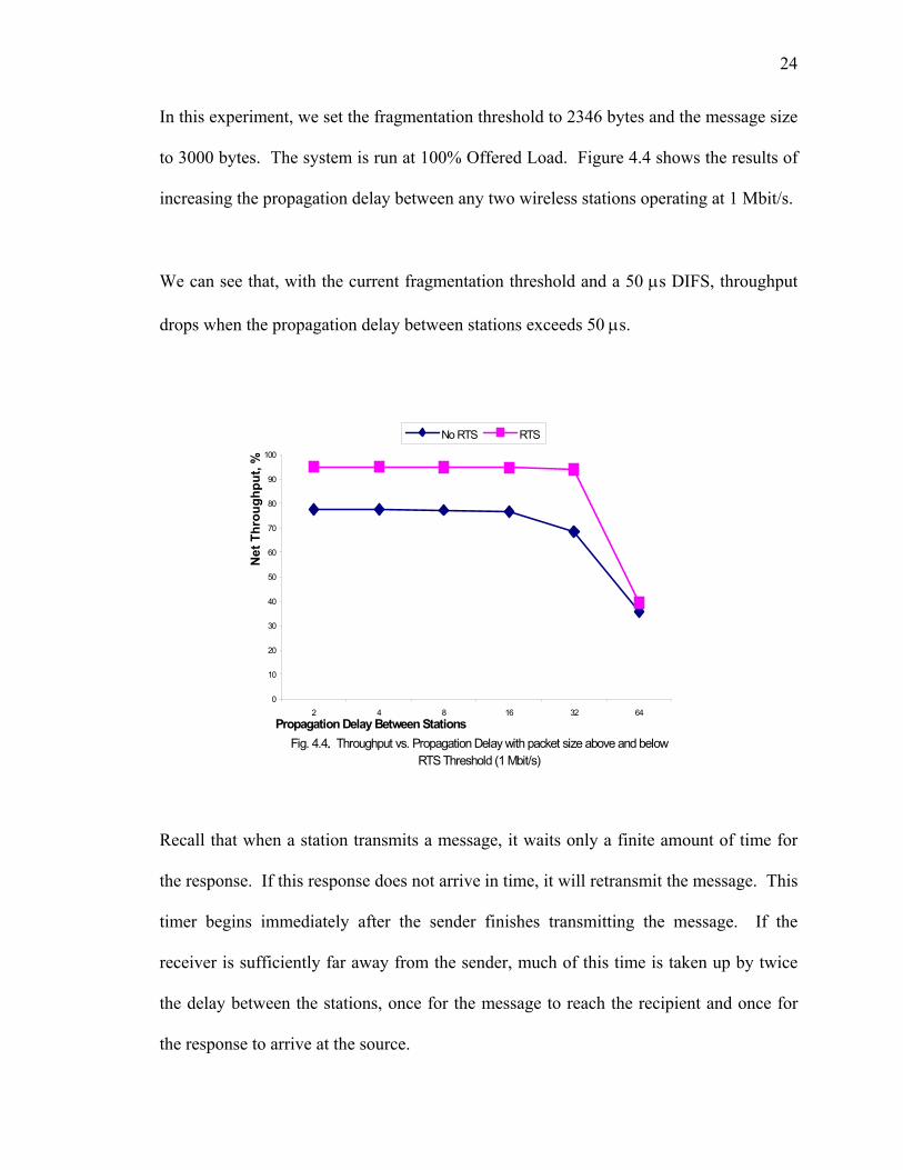
In this experiment, we set the fragmentation threshold to 2346 bytes and the message size
to 3000 bytes. The system is run at 100% Offered Load. Figure 4.4 shows the results of
increasing the propagation delay between any two wireless stations operating at 1 Mbit/s.
We can see that, with the current fragmentation threshold and a 50 µs DIFS, throughput
drops when the propagation delay between stations exceeds 50 µs.
Recall that when a station transmits a message, it waits only a finite amount of time for
the response. If this response does not arrive in time, it will retransmit the message. This
timer begins immediately after the sender finishes transmitting the message. If the
receiver is sufficiently far away from the sender, much of this time is taken up by twice
the delay between the stations, once for the message to reach the recipient and once for
the response to arrive at the source.
Fig. 4.4. Throughput vs. Propagation Delay with packet size above and below RTS Threshold (1 Mbit/s)
0
10
20
30
40
50
60
70
80
90
100
2 4 8 16 32 64Propagation Delay Between Stations
Net
Thr
ough
put,
%
No RTS RTS

25
If the distance between two stations becomes too large, it will be impossible for the
sender to hear the acknowledgement from the receiver. In this case, it becomes
increasingly difficult for messages to be received correctly. The result is increased
retransmissions and decreased throughput.
Unfortunately the problem only compounds itself as the transmission speed increases.
Figure 4.5 shows the same experiment run at 2 Mbit/s. Here we see that the same drop
off in throughput occurs with stations only 32 µs apart. The reason is that the initial
transmission is shorter at the higher speed, which forces the station to begin its waiting
period earlier. Therefore, this timer can expire with a shorter propagation delay.
Fig. 4.5. Throughput vs. Propagation Delay with packet size above and below RTS Threshold (2 Mbit/s)
0
10
20
30
40
50
60
70
80
90
100
2 4 8 16 32 64
Propagation Delay Between Stations
Net
Thr
ough
put,
%
No RTS RTS

26
As can be expected, the results are even worse for transmissions at 10 Mbit/s. These
results are shown in figure 4.6. An interesting point in all three graphs is that the RTS
mechanism can do little to improve this performance. This assures us that the loss in
throughput is not attributed to collisions but rather to too much distance between stations.
In fact, the added overhead of the RTS mechanism slightly reduces the performance once
this problem occurs.
It a reasonable assumption that there is a limit to the distance that any two
communicating stations can be from one another before system performance suffers.
This limit is based upon the attributes of the communication medium and the protocol.
From this experiment we can see that the transmission speed also plays a crucial role.
Fig. 4.6. Throughput vs. Propagation Delay with packet size above and below RTS Threshold (10 Mbit/s)
0
10
20
30
40
50
60
70
80
90
100
2 4 8 16 32 64
Propagation Delay Between Stations
Net
Thr
ough
put,
%
No RTS RTS

27
Chapter 5 Conclusion
While the experiments described in this paper do not reflect any real-life scenario, they
are useful in determining the maximum system performance under a variety of
conditions. Our goal has been to see what the maximum performance we can expect out
of the protocol is and what it takes to reach it.
We see from our experiments that Ethernet speeds are possible but only with the RTS
mechanism that is built into the 802.11 MAC protocol. This mechanism, while adding
some overhead, offers considerable improvement in most highly loaded systems.
We found that the best performance can only be achieved in systems with relatively slow
transmission speeds. Transmission speed and throughput were inversely proportional.
This is due to the constant delays and timers used in the protocol, which are not altered as
transmission speed increases.

28
Chapter 6 Future Work
Currently our research does not take into account the transmission errors that are inherent
in all forms of communication. One area of research will be to incorporate a bit-error
rate into the simulation, based upon the transmission device, and see how the system
performance is affected.
Our system did not allow for a subset of stations to be hidden from the others. We
assumed that all stations can hear all transmissions from all others. With this medium,
stations can be obstructed from some other stations in the network. This would prevent
them from reading all of the NAV values that are transmitted. Future research could take
this into account.
The aim of our research was focused on the DCF but completely ignored the optional
PCF. It is quite possible that some of the inefficiencies found in our experiments can be
overcome by the PCF.

29
Chapter 7 Bibliography
[BAN84] Banks, J. and J. S. Carson, “Discrete-Event System Simulation,” Prentice-Hall,
Englewood, NJ, 1984.
[BUX81] W. Bux, "Local-area subnetworks: A performance comparison," IEEE Trans.
Commun., vol COM-29, pp. 1465-1473, 1981.
[GON83] T. A. Gonsalves, "Performance characteristics of 2 Ethernets: An experimental
study," ACM SIGCOMM Symp. On Commun. Architectures and Protocols,
Austin, TX, Mar. 1983, pp. 178-185.
[GON87] T. A. Gonsalves, "Measured Performance of the Ethernet," in Advances in Local
Area Networks, Kummerle, K., Tobagi, F., and Limb, J.O. (Eds.), New York:
IEEE Press, 1987.
[IEE97] IEEE Std 802.11-1997, “IEEE Standard for Local and Metropolitan Area
Networks: Wireless LAN Medium Access Control (MAC) and Physical Layer
(PHY) Specification.”
[STA97] Stallings, W, "Data and Computer Communications, 5th Edition,” Prentice-Hall,
Upper Saddle River, NJ, 1997.
[TOB80] F. A. Tobagi and V. B. Hunt, "Performance analysis of carrier sense multiple
access with collision detection," Comput. Networks, vol. 4, Oct./Nov. 1980.