Approximate Verification of the Symbolic Dynamics of

HAL Id: hal-00920793https://hal.inria.fr/hal-00920793

Submitted on 18 Oct 2015

HAL is a multi-disciplinary open accessarchive for the deposit and dissemination of sci-entific research documents, whether they are pub-lished or not. The documents may come fromteaching and research institutions in France orabroad, or from public or private research centers.

L’archive ouverte pluridisciplinaire HAL, estdestinée au dépôt et à la diffusion de documentsscientifiques de niveau recherche, publiés ou non,émanant des établissements d’enseignement et derecherche français ou étrangers, des laboratoirespublics ou privés.

Approximate Verification of the Symbolic Dynamics ofMarkov Chains

Manindra Agrawal, Sundararaman Akshay, Blaise Genest, P.S. Thiagarajan

To cite this version:Manindra Agrawal, Sundararaman Akshay, Blaise Genest, P.S. Thiagarajan. Approximate Verificationof the Symbolic Dynamics of Markov Chains. Journal of the ACM (JACM), Association for ComputingMachinery, 2015, 62 (1), pp.34-65. �10.1145/2629417�. �hal-00920793�

https://hal.inria.fr/hal-00920793

https://hal.archives-ouvertes.fr

A

Approximate Verification of the Symbolic Dynamics of Markov Chains

MANINDRA AGRAWAL, Indian Institute of Technology, Kanpur, India

S. AKSHAY, Indian Institute of Technology Bombay, India

BLAISE GENEST, CNRS, UMR IRISA, Rennes, France

P. S. THIAGARAJAN, School of Computing, National University of Singapore, Singapore

A finite state Markov chain M can be regarded as a linear transform operating on the set of probability

distributions over its node set. The iterative applications of M to an initial probability distribution µ0will generate a trajectory of probability distributions. Thus a set of initial distributions will induce a set

of trajectories. It is an interesting and useful task to analyze the dynamics of M as defined by this set of

trajectories. The novel idea here is to carry out this task in a symbolic framework. Specifically, we discretizethe probability value space [0, 1] into a finite set of intervals I = {I1, I2, . . . , Im}. A concrete probability

distribution µ over the node set {1, 2, . . . , n} of M is then symbolically represented as D, a tuple of intervals

drawn from I where the ith component of D will be the interval in which µ(i) falls. The set of discretizeddistributions D is a finite alphabet. Hence the trajectory, generated by repeated applications of M to an

initial distribution, will induce an infinite string over this alphabet. Given a set of initial distributions, the

symbolic dynamics of M will then consist of an infinite language L over D.Our main goal is to verify whether L meets a specification given as a linear time temporal logic formula

ϕ. In our logic an atomic proposition will assert that the current probability of a node falls in the interval Ifrom I. Assuming L can be computed effectively, one can hope to solve our model checking problem (whether

L |= ϕ?) using standard techniques in case L is an ω-regular language. However we show that in general

this is not the case. Consequently, we develop the notion of an ε-approximation, based on the transient andlong term behaviors of the Markov chain M . Briefly, the symbolic trajectory ξ′ is an ε-approximation of the

symbolic trajectory ξ iff (1) ξ′ agrees with ξ during its transient phase; and (2) both ξ and ξ′ are within an

ε-neighborhood at all times after the transient phase. Our main results are that one can effectively checkwhether (i) for each infinite word in L, at least one of its ε-approximations satisfies the given specification;

(ii) for each infinite word in L, all its ε-approximations satisfy the specification. These verification results

are strong in that they apply to all finite state Markov chains.

Categories and Subject Descriptors: D.2.4 [Software Engineering]: Software/Program Verification—

Formal methods, Model checking; F.1.2 [Computation by Abstract Devices]: Modes of Computation—

Probabilistic computation

General Terms: Theory, Verification, Algorithms

Additional Key Words and Phrases: Markov chains, discretization, LTL logic, approximate model checking

ACM Reference Format:Agrawal, M., Akshay, S., Genest, B. and Thiagarajan, P.S. 2013. Approximate Verification of the Symbolic

Dynamics of Markov Chains J. ACM V, N, Article A (January YYYY), 32 pages.

DOI = 10.1145/0000000.0000000 http://doi.acm.org/10.1145/0000000.0000000

An extended abstract of this paper appeared at the conference Logic in Computer Science 2012.Authors’ addresses: M. Agrawal, Dept. of CSE, IIT Kanpur, India, [email protected]; S. Akshay, Dept.of CSE, IIT Bombay, Mumbai, India, [email protected]; B. Genest, CNRS, UMR IRISA, Campus deBeaulieu, Rennes, France, [email protected]; P.S.Thiagarajan, School of Computing, National University ofSingapore, Singapore, [email protected] to make digital or hard copies of part or all of this work for personal or classroom use isgranted without fee provided that copies are not made or distributed for profit or commercial advantageand that copies show this notice on the first page or initial screen of a display along with the full citation.Copyrights for components of this work owned by others than ACM must be honored. Abstracting withcredit is permitted. To copy otherwise, to republish, to post on servers, to redistribute to lists, or to use anycomponent of this work in other works requires prior specific permission and/or a fee. Permissions may berequested from Publications Dept., ACM, Inc., 2 Penn Plaza, Suite 701, New York, NY 10121-0701 USA,fax +1 (212) 869-0481, or [email protected]© YYYY ACM 0004-5411/YYYY/01-ARTA $15.00

DOI 10.1145/0000000.0000000 http://doi.acm.org/10.1145/0000000.0000000

Journal of the ACM, Vol. V, No. N, Article A, Publication date: January YYYY.

A:2

1

0.5

0 0.5 1z

y

x

Γ(.1, .6, .3)=(d1, d2, d1)

Γ(.7, .2, .1)= (d2, d1, d1)

Γ(.2, .1, .7)

= (d1, d1, d2)

Γ(.3, .3, .4)= (d1, d1, d1)

f

Fig. 1. A concrete and symbolic trajectory for a Markov chain with node set {x, y, z} projected onto thex, y plane. The discretization is {d1 = [0, 0.5), d2 = [0.5, 1]}. Here Γ is the map that sends a concretedistribution to the corresponding discretized distribution and f is the stationary distribution.

1. INTRODUCTION

Finite state Markov chains are a fundamental model of probabilistic dynamical systems.They have a rich theory [Norris 1997; Kemeny and Snell 1960] and techniques for specifyingand verifying their dynamical properties are well established [Hansson and Jonsson 1994;Baier et al. 1997; Baier et al. 2005; Baier et al. 2003; Kwiatkowska et al. 2011; Forejt et al.2011; Huth and Kwiatkowska 1997; Vardi 1999; Kwon and Agha 2004; 2011; Korthikantiet al. 2010; Chadha et al. 2011]. In a majority of the verification related studies, the Markovchain is viewed a probabilistic transition system. The paths of this transition system areviewed as computations and the goal is to use probabilistic temporal logics [Hansson andJonsson 1994; Baier et al. 2003; Huth and Kwiatkowska 1997] to reason about these com-putations.

An alternative approach -which this paper is based on- is to view the state space of theMarkov chain to be the set of probability distributions over the nodes of the chain. TheMarkov chain linearly transforms a given probability distribution into a new one. Startingfrom a distribution µ0 one iteratively applies the Markov chain M to generate a trajectoryconsisting of a sequence of distributions µ0, µ1, µ2 . . . with µk+1 = µk ·M . Given a set ofinitial distributions, the goal is to study the properties of the set of trajectories generated bythese distributions. Many interesting dynamical properties can be formulated in this settingregarding the transient and steady state behaviors of the chain. For instance one can say thatat no time will it be the case that the probability of being in the state i and the probabilityof being in the state j are both low. One can also say that starting from some stage thesystem is most likely to be in state i or state j. Additional examples of such properties arepresented in Section 3.1 for two realistic Markov chains. Such dynamical properties havealso been discussed in the literature [Kwon and Agha 2004; 2011; Korthikanti et al. 2010].

The novel idea we explore here is to study the symbolic dynamics of finite state Markovchains in this setting. We demonstrate that this is a fruitful line of enquiry by establishingan effective model checking procedure for the full class of Markov chains. Our specificationlanguage is a rich linear time temporal logic in which the atomic propositions consist ofconstraints over the intervals of probability values specified using the first order theory ofreals. Our decision procedure requires a detailed characterization of the symbolic dynam-icsby adapting and extending the existing theory of Markov chains. We expect this part ofthe work to have wider applicability.


A:3

The basic idea underlying the symbolic dynamics is the following. We discretize theprobability value space [0, 1] into a finite set of intervals I = {[0, p1), [p1, p2), . . . , [pm, 1]}.A probability distribution µ of M over its set of nodes {1, 2, . . . , n} is then representedsymbolically as a tuple of intervals (d1, d2, . . . , dn) with di ∈ I being the interval in whichµ(i) falls. Such a tuple of intervals which symbolically represents at least one probabilitydistribution is called a discretized distribution. In general, a discretized distribution willrepresent an infinite set of concrete distributions. A simple but crucial fact is that the set ofdiscretized distributions, denoted D, is a finite set. Consequently, each trajectory generatedby an initial probability distribution will induce a sequence over the finite alphabet D asillustrated in Figure 1. Hence, given a (possibly infinite) set of initial distributions IN , thesymbolic dynamics of M can be studied in terms of a language over the alphabet D. Ourfocus here is on infinite behaviors. Consequently, the main object of our study is LM,IN

(abbreviated for convenience as L), the ω-language induced by the set of distributions IN .Our main motivation for studying Markov chains in this fashion is that in many practical

applications such as biochemical networks, queuing systems or sensor networks, obtainingexact estimates of the probability distributions (including the initial distribution) may beneither feasible nor necessary. Indeed, one is often interested in properties stated in termsof probability ranges, such as “low, medium or high” or “above the threshold 0.8” ratherthan exact values. We note that the discretization of [0, 1] need not be the same alongeach dimension. Specifically, if a node is not relevant for the question at hand we canfilter it out by associating the “don’t care” discretization {[0, 1]} with it. This dimensionreduction technique can significantly reduce the practical complexity of analyzing highdimensional Markov chains. Last but not least, a variety of formal verification techniquesthat are available for studying languages over finite alphabets can be deployed. Indeed thiswill be the main technical focus of this paper.

In particular, we formulate a linear time temporal logic in which an atomic propositionwill assert that “the current probability of the node i lies in the interval d”. The rest of thelogic is obtained by closing under propositional connectives and the temporal modalitiesnext and until in the usual way. We have chosen this simple logic in order to highlight themain ideas. As pointed out in Section 3 this logic can be considerably enriched and ourtechniques will easily extend -albeit with additional computational costs- to this enrichedversion. Using results available in the literature [Beauquier et al. 2002; Korthikanti et al.2010] we also show that our logic’s expressive power is incomparable with logics such asPCTL interpreted over the paths of the Markov chain.

Based on our logic, the key model checking question we address is whether each sequencein L is a model of the specification ϕ. If L is an effectively computable ω-regular language,then standard model checking techniques can be applied to answer this question. Usingbasic results from complex analysis and algebraic number theory we show however that L isnot ω-regular in general. This turns out to be the case even if we restrict M to be irreducibleand aperiodic. This well-known structural restriction (defined in Section 2) guarantees thatthere is a unique probability distribution µf such that for every distribution µ, the trajectorystarting from µ will converge to µf .

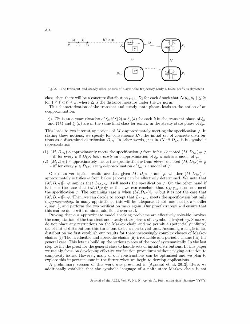
To get around this we construct two closely related approximate solutions to our verifi-cation problem. We fix an approximation factor ε > 0. We then show that each symbolictrajectory can be split into a transient phase and a steady state phase as illustrated inFigure 2. Further, if ξµ is the symbolic trajectory induced by the initial distribution µ, thenin the steady state phase, ξµ will cycle through a set of final classes {F0,F1, . . . ,Fθ−1}where each Fm is a set of discretized distributions. Intuitively, these final classes will eachcorrespond to the periodic components of the Markov chain with θ defining the period ofM as formalized later in the paper. Finally, the discretized distributions constituting a finalclass will be close to each other in the following sense: if F = {D1, D2, . . . , Dk} is a final


A:4

µ µ1

Mµ2

MM

MM

F0 F1

F2Fθ−1

Kǫ steps

ǫ

ǫ

Fig. 2. The transient and steady state phases of a symbolic trajectory (only a finite prefix is depicted)

class, then there will be a concrete distribution µ` ∈ D` for each ` such that ∆(µ`, µ`′) ≤ 2εfor 1 ≤ ` < `′ ≤ k, where ∆ is the distance measure under the L1 norm.

This characterization of the transient and steady state phases leads to the notion of anε-approximation:

— ξ ∈ Dω is an ε-approximation of ξµ if ξ(k) = ξµ(k) for each k in the transient phase of ξµ;and ξ(k) and ξµ(k) are in the same final class for each k in the steady state phase of ξµ.

This leads to two interesting notions of M ε-approximately meeting the specification ϕ. Instating these notions, we specify for convenience IN , the initial set of concrete distribu-tions as a discretized distribution DIN . In other words, µ is in IN iff DIN is its symbolicrepresentation.

(1) (M,DIN ) ε-approximately meets the specification ϕ from below - denoted (M,DIN )|=εϕ

- iff for every µ ∈ DIN , there exists an ε-approximation of ξµ which is a model of ϕ.

(2) (M,DIN ) ε-approximately meets the specification ϕ from above -denoted (M,DIN )|=ε ϕ- iff for every µ ∈ DIN , every ε-approximation of ξµ is a model of ϕ.

Our main verification results are that given M , DIN , ε and ϕ, whether (M,DIN ) ε-approximately satisfies ϕ from below (above) can be effectively determined. We note that(M,DIN )|=ε ϕ implies that LM,DIN

itself meets the specification ϕ. On the other hand ifit is not the case that (M,DIN )|=

εϕ then we can conclude that LM,DIN

does not meetthe specification ϕ. The remaining case is when (M,DIN )|=

εϕ but it is not the case that

(M,DIN )|=ε ϕ. Then, we can decide to accept that LM,DIN meets the specification but onlyε-approximately. In many applications, this will be adequate. If not, one can fix a smallerε, say, ε

2 , and perform the two verification tasks again. Our proof strategy will ensure thatthis can be done with minimal additional overhead.

Proving that our approximate model checking problems are effectively solvable involvesthe computation of the transient and steady state phases of a symbolic trajectory. Since wedo not place any restrictions on the Markov chain and we permit a (potentially infinite)set of initial distributions this turns out to be a non-trivial task. Assuming a single initialdistribution we first establish our results for three increasingly complex classes of Markovchains: (i) The irreducible and aperiodic chains (ii) irreducible and periodic chains (iii) thegeneral case. This lets us build up the various pieces of the proof systematically. In the laststep we lift the proof for the general class to handle sets of initial distributions. In this paperwe mainly focus on developing effective verification procedures without paying attention tocomplexity issues. However, many of our constructions can be optimized and we plan toexplore this important issue in the future when we begin to develop applications.

A preliminary version of this work was presented in [Agrawal et al. 2012]. Here, weadditionally establish that the symbolic language of a finite state Markov chain is not


A:5

always ω-regular by using basic algebraic number theory and complex analysis. We alsoformally extend our logic using the first order theory of reals and develop two detailedexamples to illustrate our approach.

1.1. Related work:

Symbolic dynamics is a classical topic in the theory of dynamical systems [Morse andHedlund 1938] with data storage, transmission and coding being the major applicationareas [Lind and Marcus 1995]. The basic idea is to partition the “smooth” state space intoa finite set of blocks and represent a trajectory as a sequence of such blocks. In terms offormal verification terminology a crucial assumption is that this set of partitions induces abisimulation equivalence over the dynamics in the sense that if two states s and s′ lie in thesame partition then T (s) and T (s′) will also lie in the same partition where T is the statetransformation function associated with the dynamical system. Consequently one can usethe notion of shift sequences and shifts of finite type to study the symbolic dynamics[Lindand Marcus 1995]. In our setting the partitioning induced by the discretization of [0, 1]will not be a bisimulation (except for the degenerate discretization {[0, 1]}). Consequentlythe resulting symbolic dynamics will be a lot more complicated. Indeed, the bulk of thetechnical aspects of our work is devoted to overcoming this hurdle.

Markov chains have been intensely studied (see for instance [Kemeny and Snell 1960;Norris 1997; Lalley 2010; Meyn and Tweedie 1993]). Among the main results are uniformconvergence theorems which describe how an irreducible and aperiodic chain converges to-wards a unique stationary distribution. However, general Markov chains do not always haveunique stationary distributions and other notions of convergence such as Cesaro convergencehave sometimes been used to study them. In our treatment of irreducible and aperiodicchains we do appeal to uniform convergence results taken from the literature. However ourfocus is decidability of the approximate model checking problem in the symbolic dynam-ics setting. Hence we work with weaker bounds on the rates of convergence, that can beextended to all Markov chains and which will in addition work for a (potentially infinite)set of initial distributions. To derive these bounds, we develop new techniques based on theexisting theory of Markov chains as well as the graph decomposition based model checkingtechniques described in [Baier and Katoen 2008].

Our discretization resembles the ones used in timed automata [Alur and Dill 1994] andhybrid automata [Henzinger 1996]. There are however two crucial differences. In our settingthere are no resets involved and there is just one mode, namely the linear transform M ,driving the dynamics. On the other hand, for timed automata and hybrid automata thegoal is to find a discretization that leads to a bisimulation of finite index over the set oftrajectories. Further, almost always this is obtained only in cases when the dynamics of thevariables are decoupled from each other. In our setting this will be an untenable restriction.Consequently we cannot readily use results concerning timed and hybrid automata to studyour symbolic dynamics.

Viewing a Markov chain as a transform of probability distributions and verifying theresulting dynamics has been explored previously [Kwon and Agha 2004; 2011; Korthikantiet al. 2010; Chadha et al. 2011]. To be precise, the work reported in [Korthikanti et al.2010; Chadha et al. 2011] deals with MDPs (Markov Decison Processes) instead of Markovchains. However by considering the case where the MDP accesses just one Markov chain wecan compare our work with theirs. Firstly [Kwon and Agha 2004; Korthikanti et al. 2010;Chadha et al. 2011] consider only one initial distribution and hence just one trajectoryneeds to be analyzed. It is difficult to see how their results can be extended to handlemultiple -and possibly infinitely many- initial distributions as we do. Secondly, they studyonly irreducible and aperiodic Markov chains. In contrast we consider the class of all Markovchains. Last but not least, they impose the drastic restriction that the unique fix point ofthe irreducible and aperiodic Markov chain is an interior point w.r.t. the discretization


A:6

induced by the specification. In [Chadha et al. 2011], a similar restriction is imposed in aslightly more general setting. Since the fix point is determined solely by the Markov chainand is unrelated to the specification, this is not a natural restriction. As we point out inSection 6 we can also easily obtain an exact solution to our model checking problem byimposing such a restriction.

Returning to the two approaches to studying Markov chains, a natural question to askis how they are related. It turns out that from a verification standpoint they are incom-parable and complementary (see [Beauquier et al. 2002; Korthikanti et al. 2010]). Further,solutions to model checking problems in one approach (e.g. the decidability of PCTL inthe probabilistic transition system setting) will not translate into the other. Finally, inter-vals of probability distributions have been considered previously in a number of settings[Weichselberger 2000; Skulj 2009; Kozine 2002; Jonsson and Larsen 1991; Delahaye et al.2011; Chatterjee et al. 2008; Haddad and Pekergin 2009]. In these studies the resultingobjects, often called interval Markov chains, use intervals of probability distributions tocapture uncertainties in the transition probabilities. One then essentially studies a convexset of Markov chains using an envelope of upper and lower probability distributions. In oursetting, we focus instead on uncertainties associated with the probability distributions overthe states of a Markov chain. Furthermore we use a fixed discretization over [0, 1] to modelthis and develop an approximate verification procedure for the resulting symbolic dynamics.It will however be interesting to extend our results and techniques to the setting of intervalMarkov chains.

We discovered recently (while preparing the final version of this manuscript) that thenon-regularity of languages associated with finite state Markov chains has been studiedpreviously in [Turakainen 1968] in the setting of languages of probabilistic automata overa single-letter alphabet. This study also uses algebraic techniques very similar to ours.However only languages over finite words are considered. More importantly, the dynamicsstudied consists of a language over a one letter alphabet that tracks the number of times thechain has been applied to an initial distribution to reach a final distribution in which theprobability mass of a designated subset of final nodes exceeds a fixed threshold value. Ourdynamics tracks the distribution itself in a symbolic manner using the notion of discretizeddistributions.

1.2. Plan of the paper:

In the next section, we define the notion of discretized distributions and the symbolicdynamics of Markov chains. In Section 3, we introduce our temporal logic, illustrate itsexpressiveness and show how it can be extended. In the subsequent section, we present aMarkov chain consisting of 3 nodes and prove that its symbolic dynamics is not ω-regular. InSection 5 we formulate our main approximate model checking results and then in the subse-quent sections establish these results systematically. In Section 6, we handle irreducible andaperiodic Markov chains and in Section 7 irreducible but periodic chains. In the subsequentsection general Markov chains are treated. In order to highlight the key technical issues, inthese sections we consider just one initial concrete distribution. In Section 9, we handle aset of initial concrete distributions. In the concluding section we summarize our results andpoint to future research directions.

2. SYMBOLIC DYNAMICS

We begin with Markov chains. Through the rest of the paper we fix a finite set of nodesX = {1, 2, . . . , n} and let i, j range over X . As usual a probability distribution over X ,is a map µ : X → [0, 1] such that

∑i µ(i) = 1. Henceforth we shall refer to such a µ

as a distribution and sometimes as a concrete distribution. We let µ, µ′ etc. range overdistributions. A Markov chain M over X will be represented as an n× n matrix with non-negative entries satisfying

∑jM(i, j) = 1 for each i. Thus, if the system is currently at


A:7

node i, then M(i, j) is the probability of it being at j in the next time instant. We will saythat M transforms µ into µ′, if µ ·M = µ′.

We will often appeal to basic notions and results about Markov chains without explicitreferences. They can be found in any of the standard references [Norris 1997; Kemenyand Snell 1960]. In particular we will need the notions of irreducibility, aperiodicity andperiodicity.

Let M be a Markov chain over X = {1, 2, . . . , n}. The graph of M is the directed graphGM = (X , E) with (i, j) ∈ E iff M(i, j) > 0. We say that M is irreducible in case GMis strongly connected. Assume M is irreducible. The period of the node i is the smallestinteger mi such that Mmi(i, i) > 0. The period of M is denoted as θM and it is the greatestcommon divisor of {mi}i∈X . The irreducible Markov chain M is said to be aperiodic ifθM = 1. Otherwise, it is periodic. While we will use these notions throughout the paper, wewish to emphasize that the model checking results of the paper will nevertheless apply forall Markov chains.

2.1. The discretization

We fix a partition of [0, 1] into a finite set I of intervals and call it a discretization. We letd, d′ etc. range over I. Suppose D : X → I. Then D is a discretized distribution iff thereexists a concrete distribution µ : X → [0, 1] such that µ(i) ∈ D(i) for every i. We denoteby D the set of discretized distributions, and let D, D′ etc. range over D. A discretizeddistribution will sometimes be referred to as a D-distribution. We often view D as an n-tuple D = (d1, d2, . . . , dn) ∈ In with D(i) = di.

Suppose n = 3 and I = {[0, 0.2), [0.2, 0.4), [0.4, 0.7), [0.7, 1]}. Then, the 3-tuple([0.2, 0.4), [0.2, 0.4), [0.4, 0.7)) is a D-distribution since for the concrete distribution(0.25, 0.30, 0.45), we have 0.25, 0.30 ∈ [0.2, 0.4) while 0.45 ∈ [0.4, 0.7). On the other hand,neither ([0, 0.2), [0, 0.2), [0.2, 0.4)) nor ([0.4, 0.7), [0.4, 0.7), [0.7, 1]) are D-distributions.

We have fixed a single discretization and applied it to each dimension to reduce notationalclutter. As stated in the introduction, in applications, it will be useful to fix a differentdiscretization Ii for each i. In this case one can set Ii = {[0, 1]} for each “don’t care” nodei. Our results will go through easily in such settings.

A concrete distribution µ can be abstracted as a D-distribution D via the map Γ givenby: Γ(µ) = D iff µ(i) ∈ D(i) for every i. Since I is a partition of [0, 1] we are assuredthat Γ is well-defined. Intuitively, we do not wish to distinguish between µ and µ′ in caseΓ(µ) = Γ(µ′). Note that D is a non-empty and finite set. By definition we also have thatΓ−1(D) is a non-empty set of distributions for each D. Abusing notation -as we have beendoing already- we will often view D as a set of concrete distributions and write µ ∈ D (orµ is in D etc.) instead of µ ∈ Γ−1(D).

We focus on infinite behaviors. With suitable modifications, all our results can be special-ized to finite behaviors. A trajectory of M is an infinite sequence of concrete distributionsµ0µ1 . . . such that µl ·M = µl+1 for every l ≥ 0. We let TRJM denote the set of trajectoriesof M (we will often drop the subscript M). As usual for ρ ∈ TRJ with ρ = µ0µ1 . . ., we shallview ρ as a map from {0, 1, . . .} into the set of distributions such that ρ(l) = µl for everyl. We will follow a similar convention for members of Dω, the set of infinite sequences overD. Each trajectory induces an infinite sequence of D-distributions via Γ. More precisely, wedefine Γω : TRJ → Dω as Γω(ρ) = ξ iff Γ(ρ(`)) = ξ(`) for every `. In what follows we willwrite Γω as just Γ.

Given an initial set of concrete distributions, we wish to study the symbolic dynamicsof M induced by this set of distributions. For convenience, we shall specify the set ofinitial distributions as a D-distribution DIN . In general, DIN will contain an infinite setof distributions. In the example introduced above, ([0.2, 0.4), [0.2, 0.4), [0.4, 0.7)) is such adistribution. Our results will at once extend to sets of D-distributions.


A:8

We now define LM,DIN = {ξ ∈ Dω | ∃ρ ∈ TRJ , ρ(0) ∈ DIN , Γ(ρ) = ξ}. We view LM,DIN

to be the symbolic dynamics of the system (M,DIN ) and refer to its members as symbolictrajectories. From now on, we will write LM instead of LM,DIN

since DIN will be clear fromthe context. Given (M,DIN ), our goal is to specify and verify properties of LM .

3. THE MODEL CHECKING PROBLEM

The properties of the symbolic dynamics of M will be formulated using probabilistic lin-ear time temporal logic LTLI . The set of atomic propositions is denoted AP and is given by:

AP = {〈i, d〉 | 1 ≤ i ≤ n, d ∈ I}.

The atomic proposition 〈i, d〉 asserts that D(i) = d where D is the current discretizeddistribution of M . The formulas of LTLI are:

— Every atomic proposition as well as the constants tt and ff are formulas.— If ϕ and ϕ′ are formulas then so are ¬ϕ and ϕ ∨ ϕ′.— If ϕ is a formula then Xϕ is a formula.— If ϕ and ϕ′ are formulas then ϕUϕ′ is a formula.

The propositional connectives such as ∧, → and ≡ are derived in the usual way as alsothe “future” modality 3ϕ = ttUϕ. This leads to the “always” modality 2ϕ = (¬3¬ϕ).

The semantics of the logic is given in terms of the satisfaction relation ξ, l |= ϕ, whereξ ∈ Dω, l ≥ 0 and ϕ is a formula. This relation is defined inductively via:

— ξ, l |= 〈i, d〉 iff ξ(l)(i) = d— The constants tt and ff as well as the connectives ¬ and ∨ are interpreted as usual.— ξ, l |= Xϕ iff ξ, (l + 1) |= ϕ— ξ, l |= ϕUϕ′ iff there exists k ≥ l such that ξ, k |= ϕ′ and ξ, l′ |= ϕ for l ≤ l′ < k.

We say that ξ is a model of ϕ iff ξ, 0 |= ϕ. In what follows, Lϕ will denote the set ofmodels of ϕ. Further, for a distribution µ we let ρµ denote the trajectory in TRJ whichsatisfies: ρ(0) = µ. Finally, we let ξµ = Γ(ρµ) be the symbolic trajectory generated by µ.M,DIN |= ϕ will denote that (M,DIN ) meets the specification ϕ and it holds iff ξµ ∈ Lϕ

for every µ ∈ DIN . In other words, LM ⊆ Lϕ. Given a finite state Markov chain M ,a discretization I, an initial set of concrete distributions DIN and a specification ϕ, themodel checking problem is to determine whether M,DIN |= ϕ.

Before proceeding to solve this model checking problem, we shall first consider what canbe specified in our logic.

3.1. Expressiveness issues

In our logic the formula∧i〈i, di〉 can be used to assert that the current D-distribution is

D = (d1, d2, . . . , dn). We can assertD will be encountered infinitely often via (23〈D〉) where〈D〉 is an abbreviation for

∧i〈i,D(i)〉. We can also assert that the set of D-distributions

that appear infinitely often is from a given subset D′ of D via 32∨D∈D′〈D〉. One can easily

strengthen this formula to assert that the set of D-distributions that appear infinitely oftenis exactly D′.

Next, we can classify members of I as representing “low” and “high” probabilities. Forexample, if I contains 10 intervals each of length 0.1, we can declare the first two intervals as“low” and the last two intervals as “high”. In this case 2(〈i, d9〉∨ 〈i, d10〉 → 〈j, d1〉∨ 〈j, d2〉)will say that “whenever the probability of i is high, the probability of j will be low”. Wenow exhibit two practical settings where our approach can lead to valuable insights.

3.1.1. Example 1: The PageRank algorithm. The Google PageRank algorithm runs on a sim-plified Markov chain model P of the web. As explained in Chapter 11.6 of [Mieghem 2006],


A:9

1

2

3

4

5

13

13

13

13

12

13

12 1

13

180

1960

340

1960

67240

180

120

41120

1960

67240

116

14

38

14

116

180

120

78

120

180

3380

920

340

120

180

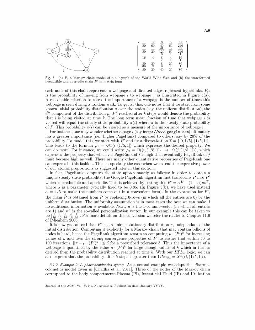
Fig. 3. (a) P , a Markov chain model of a subgraph of the World Wide Web and (b) the transformedirreducible and aperiodic chain P ′ in matrix form

each node of this chain represents a webpage and directed edges represent hyperlinks. Pijis the probability of moving from webpage i to webpage j as illustrated in Figure 3(a).A reasonable criterion to assess the importance of a webpage is the number of times thiswebpage is seen during a random walk. To get at this, one notes that if we start from someknown initial probability distribution µ over the nodes (say, the uniform distribution), theith component of the distribution µ ·P k reached after k steps would denote the probabilitythat i is being visited at time k. The long term mean fraction of time that webpage i isvisited will equal the steady-state probability π(i) where π is the steady-state probabilityof P . This probability π(i) can be viewed as a measure of the importance of webpage i.

For instance, one may wonder whether a page i (say http://www.google.com) ultimatelyhas a greater importance (i.e., higher PageRank) compared to others, say by 20% of theprobability. To model this, we start with P ′ and fix a discretization I = {[0, 1/5], (1/5, 1]}.This leads to the formula ϕ1 = 32〈i, (1/5, 1]〉 which expresses the desired property. Wecan do more. For instance, we could write ϕ2 = 2(〈i, (1/5, 1]〉 → 3〈j, (1/5, 1]〉), whichexpresses the property that whenever PageRank of i is high then eventually PageRank of jmust become high as well. There are many other quantitative properties of PageRank onecan express in this fashion. This is especially the case when we extend the expressive powerof our atomic propositions as suggested later in this section.

In fact, PageRank computes the state approximately as follows: in order to obtain aunique steady-state probability, the Google PageRank algorithm first transforms P into P ′

which is irreducible and aperiodic. This is achieved by setting this P ′ = αP + (1− α)uvT ,where α is a parameter typically fixed to be 0.85. (In Figure 3(b), we have used insteadα = 4/5 to make the numbers come out in a convenient form). In the expression for P ′,

the chain P is obtained from P by replacing 0-rows (in which all the entries are 0) by theuniform distribution. The uniformity assumption is in most cases the best we can make ifno additional information is available. Next, u is the 1-column-vector (in which all entriesare 1) and vT is the so-called personalization vector. In our example this can be taken tobe [ 1

16416

616

416

116 ]. For more details on this conversion we refer the reader to Chapter 11.6

of [Mieghem 2006].It is now guaranteed that P ′ has a unique stationary distribution π, independant of the

initial distribution. Computing it explicitly for a Markov chain that may contain billions ofnodes is hard, hence the PageRank algorithm resorts to computing µ · (P ′)k for increasingvalues of k and uses the strong convergence properties of P ′ to ensure that within 50 to100 iterations, ||π − µ · (P ′)k|| ≤ δ for a prescribed tolerance δ. Thus the importance of awebpage is quantified by the value µ · (P ′)k for large enough values of k which in turn isderived from the probability distribution reached at time k. With our LTLI logic, we canalso express that the probability after k steps is greater than 1/5: ϕ3 = Xk(〈i, (1/5, 1]〉).

3.1.2. Example 2: A pharmacokinetics system. As a second example we adapt the Pharma-cokinetics model given in [Chadha et al. 2011]. Three of the nodes of the Markov chaincorrespond to the body compartments Plasma (Pl), Intersticial Fluid (IF) and Utilization


A:10

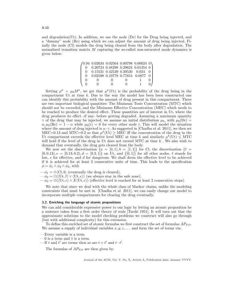
and degradation(Ut). In addition, we use the node (Dr) for the Drug being injected, anda “dummy” node (Re) using which we can adjust the amount of drug being injected. Fi-nally the node (Cl) models the drug being cleared from the body after degradation. Thenormalized transition matrix M capturing the so-called non-saturated mode dynamics isgiven below:

0.94 0.02634 0.02564 0.00798 0.00024 00 0.20724 0.48298 0.29624 0.01354 00 0.15531 0.42539 0.39530 0.024 00 0.02598 0.10778 0.77854 0.0877 00 0 0 0 1 00 0 0 0 1 0

Setting µk = µ0M

k, we get that µk(Ut) is the probability of the drug being in thecompartment Ut at time k. Due to the way the model has been been constructed onecan identify this probability with the amount of drug present in this compartment. Thereare two important biological quantities: The Minimum Toxic Concentration (MTC) whichshould not be exceeded, and the Minimum Effective Concentration (MEC) which needs tobe reached to produce the desired effect. These quantities are of interest in Ut, where thedrug produces its effect -if any- before getting degraded. Assuming a maximum quantityγ of the drug that may be injected, we assume an initial distribution µ0, with µ0(Dr) =α, µ0(Re) = 1 − α while µ0(i) = 0 for every other node i. This will model the situationwhere the amount of drug injected is α ·γ. As suggested in [Chadha et al. 2011], we then setMEC=0.13 and MTC=0.2 so that µk(Ut) ≥ MEC iff the concentration of the drug in theUt compartment exceeds the effective level MEC at time k and similarly µk(Ut) ≤ MTCwill hold if the level of the drug in Ut does not exceed MTC at time k . We also wish todemand that eventually, the drug gets cleared from the body.

We now set the discretization {a = [0, 1), b = [1, 1]} for Cl, the discretization {` =[0, 0.13), e = [0.13, 0.2), d = [0.2, 1]} on Ut, and {[0, 1]} for all other nodes. ` stands forlow, e for effective, and d for dangerous. We shall deem the effective level to be achievedif it is achieved for at least 2 consecutive units of time. This leads to the specificationφ = φ1 ∧ φ2 ∧ φ3, with

— φ1 = 3〈Cl, b〉 (eventually the drug is cleared),— φ2 = 2(〈Ut, `〉 ∨ 〈Ut, e〉) (we always stay in the safe zone),— φ3 = 3(〈Ut, e〉 ∧X〈Ut, e〉) (effective level is reached for at least 2 consecutive steps).

We note that since we deal with the whole class of Markov chains, unlike the modelingconstraints that must be met in [Chadha et al. 2011], we can easily change our model toincorporate multiple compartments for clearing the drug eventually.

3.2. Enriching the language of atomic propositions

We can add considerable expressive power to our logic by letting an atomic proposition bea sentence taken from a first order theory of reals [Tarski 1951]. It will turn out that theapproximate solutions to the model checking problems we construct will also go through(but with additional complexity) for this extension.

To define this enriched set of atomic formulas we first construct the set of formulas APFO.We assume a supply of individual variables x, y, z, . . . and form the set of terms via:

— Every variable is a term.— 0 is a term and 1 is a term.— If t and t′ are terms then so are t+ t′ and t · t′.

The formulas of APFO are then given by:


A:11

— If t is a term then 〈i, t〉 is a formula.— If t and t′ are terms then t ≤ t′ is an atomic formula.— If χ and χ′ are formulas then so are ¬χ and χ ∨ χ′.— If χ is a formula then (∃x)χ is a formula.

A structure for this language is a discretized distribution D = (d1, d2, . . . , dn). An in-terpretation is a function I which assigns a rational number to every variable while theconstant symbols 0 and 1 are assigned their standard interpretation. I extends uniquelyto the set of terms and by abuse of notation this extension will also be denoted as I. Thenotion of D being a model of the formula χ under the interpretation I is denoted D |=I

FO χand defined via:

—D |=IFO 〈i, t〉 iff I(t) ∈ D(i).

—D |=IFO t ≤ t′ iff I(t) ≤ I(t′).

—D |=IFO ¬χ iff D 6|=I

FO χ—D |=I

FO χ ∨ χ′ iff D |=IFO χ or D |=I

FO χ′

—D |=IFO (∃x)χ iff there exists a rational number c and an interpretation I′ such that

D |=I′

FO χ and I′ satisfies: I′(y) = c if y = x and I′(y) = I(y) otherwise.

The notions of free and bound occurrences of the variables in a formula are defined inthe usual way. A sentence is a formula which has no free occurrences of variables in it. If χis a sentence then we will write D |=FO χ to indicate that D is a model of χ.

In the extended logic, AP , the set of atomic propositions, is the set of sentences in theabove language. The other parts of the syntax remain unchanged. In this setting AP willbe an infinite set. However a specification can mention only a finite number of atomicpropositions and hence this will pose no problems. The semantics is given as follows. Letξ ∈ Dω, l ≥ 0 and ap be an atomic proposition. Then:

— ξ, l |= ap iff ξ(l) |=FO ap

All other cases are treated as in the original semantics. We can now formulate a muchricher variety of quantitative assertions. For instance we can assert that eventually morethan 90% of the probability mass will accumulate in the nodes 1 and 2 of the chain via:

32(∀x1∀x2 . . . ∀xn)(dist(x1, x2, . . . , xn)→ ((x1 + x2) > 0.9)).

Here dist(x1, x2, . . . , xn) is an abbreviation for the formula∧i〈i, xi〉∧(x1 +x2 + . . . xn = 1).

3.3. Relationship to other logics

A natural question that arises is how LTLI - interpreted over trajectories of probabilitydistributions - is related to logics interpreted over the paths of a Markov chain. As mentionedin the introduction, these two families of logics are incomparable. This follows from thereasoning as in [Beauquier et al. 2002]. Further our logic and the logic of probabilitiesdefined in [Beauquier et al. 2002] are incomparable by a similar reasoning as in [Korthikantiet al. 2010]. A detailed comparison between our work and that of [Korthikanti et al. 2010]has been given in Section 1.1, but we reiterate here that by fixing our discretization fromthe given formula we can express any property in their logic.

We now compare with PCTL∗, which cannot express properties which are defined acrossseveral paths of the same length in the execution of a Markov chain. For instance, inour setting, consider the formula ψ1 = 3〈i, [1, 1]〉 which says that there is future timepoint at which the probability of occupying node i is 1. Intuitively this will be impossibleto express in PCTL∗ since the probability of node i at time point t will be the sum ofprobabilities accumulated at i through several paths. For a formal proof that this statementcannot be expressed in PCTL∗, we refer the reader to [Beauquier et al. 2002]. However,


A:12

1

2

P

3

4

5

Q

1/2

1/2

1/4

1/4

3/4

3/4

1

1

Ma

1

2

P

3

4

5

Q

1/2

1/2

1

1

1

1

Mb

Fig. 4. Markov chains distinguishable by PCTL∗ formulas

to provide some intuition, notice for instance that the PCTL∗ (in fact PCTL) formulaψ2 = P≥1(tt U ati), where ati is an atomic proposition that holds only at i, does not modelthe property. Consider the Markov chain over three states i, j, k which has probability 1/3to go from any state to any state and define the discretization to be I = {d1 = [0, 1/2), d2 =[1/2, 1), d3 = [1, 1]}. Then starting from the discretized distribution (d1, d1, d1) (with e.g.concrete distribution (1/3, 1/3, 1/3)), the symbolic trajectory will be (d1, d1, d1)ω: one willnever reach (d3, ∗, ∗) (in fact, not even (d2, ∗, ∗) can be reached). That is, the LTLI formulaψ1 does not hold from (d1, d1, d1). However, the PCTL∗ (and PCTL) formula ψ2 holdsfrom each state i, j, k, hence it holds from every concrete distribution of (d1, d1, d1) (forinstance (1/3, 1/3, 1/3)). Note further that this discrepency is not restricted to singletonintervals, since by the same argument a property such as 3〈i, [1/2, 2/3]〉 cannot be expressedin PCTL∗.

On the other hand, there are properties expressible in PCTL∗ which cannot be expressedin our logic LTLI . This has been essentially established in the setting of [Korthikantiet al. 2010]. Consider the Markov chains Ma and Mb in Figure 4. Since they exhibit thesame infinite sequences of distributions they cannot be distinguished by our logic. However,consider the PCTL∗ (in fact, PCTL) formula ϕ1 = Prob≥1/8(X(P U Q)) where P,Q arepredicates that hold only at nodes 2 and 5 respectively, and the starting state is fixed tobe state 1. Then, Ma satisfies ϕ1 (the set of paths starting with the prefix 1, 2, 5 havemeasure 3/8) but Mb does not (no path visits 2 and then 5). Thus, ϕ1 is not expressible inLTLI . Intuitively, PCTL∗ formulas can describe the ‘branching’ nature of the paths baseddynamics which our logic cannot.

Next the logic of probabilities considered in [Beauquier et al. 2002] is incompara-ble with LTLI . If we consider the Markov chains in Figure 4 and the property ϕ2 =Prob>1/8(∃t, t′(t < t′) ∧ P (t) ∧ Q(t′)) in the logic of probabilities, this distinguishes Ma

from Mb and cannot be expressed in our logic. On the other hand our logic is at least asexpressive as the one used in [Korthikanti et al. 2010] as pointed out earlier. Hence itfollows from [Korthikanti et al. 2010] that there exists a formula in our logic which is notexpressible in the logic of probabilities studied in [Beauquier et al. 2002].

3.4. Discretizations based on specifications

In our logic we have fixed a discretization first and designed the set of atomic propositionsto be compatible with it. Alternatively we could have started with a temporal logic whichmentions point values of probabilities. It is then easy to fix all the probability values men-tioned in the formulas as interval end points to derive a discretization. This is similar tothe way regions and zones are derived in timed automata.

We however feel that fixing a discretization independent of specifications and studyingthe resulting symbolic dynamics is a fruitful approach. Indeed, the discretization will oftenbe a crucial part of the modeling phase. One can then, if necessary, further refine thediscretization in the verification phase.


A:13

1 2

3

0.1

0.3

0.3

0.10.1

0.3

0.6 0.6

0.6

M1 =

(

0.6 0.1 0.30.3 0.6 0.10.1 0.3 0.6

)

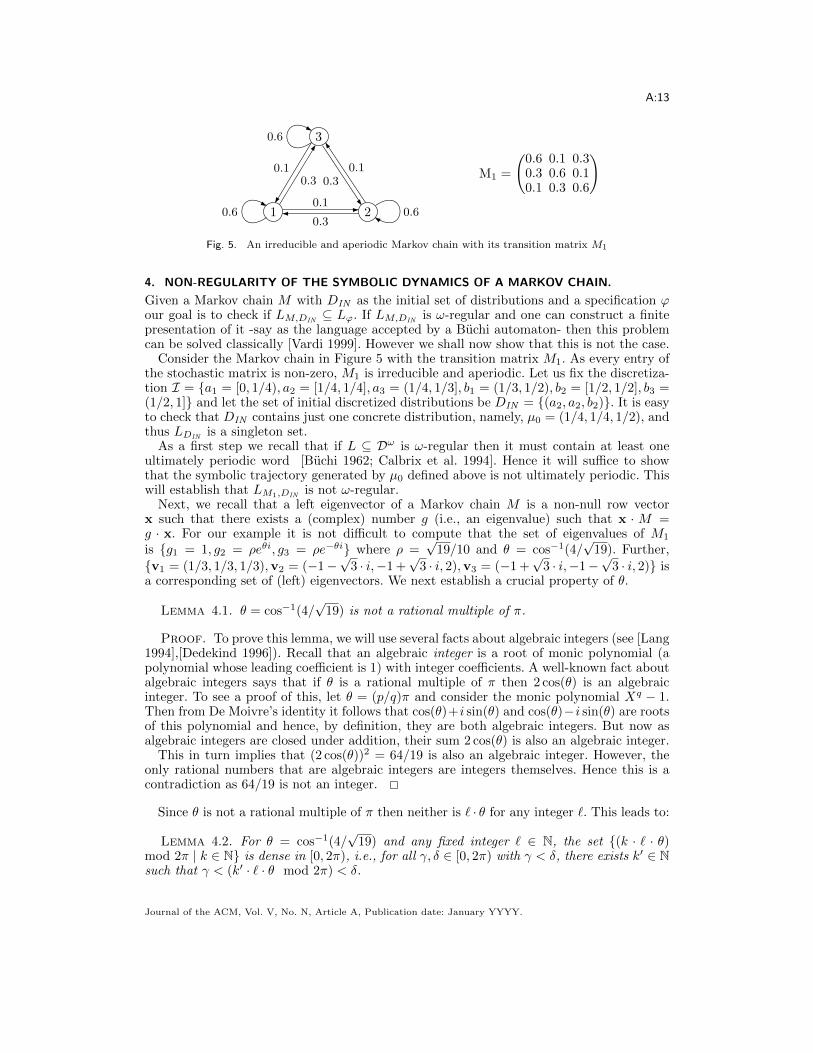
Fig. 5. An irreducible and aperiodic Markov chain with its transition matrix M1

4. NON-REGULARITY OF THE SYMBOLIC DYNAMICS OF A MARKOV CHAIN.

Given a Markov chain M with DIN as the initial set of distributions and a specification ϕour goal is to check if LM,DIN ⊆ Lϕ. If LM,DIN is ω-regular and one can construct a finitepresentation of it -say as the language accepted by a Buchi automaton- then this problemcan be solved classically [Vardi 1999]. However we shall now show that this is not the case.

Consider the Markov chain in Figure 5 with the transition matrix M1. As every entry ofthe stochastic matrix is non-zero, M1 is irreducible and aperiodic. Let us fix the discretiza-tion I = {a1 = [0, 1/4), a2 = [1/4, 1/4], a3 = (1/4, 1/3], b1 = (1/3, 1/2), b2 = [1/2, 1/2], b3 =(1/2, 1]} and let the set of initial discretized distributions be DIN = {(a2, a2, b2)}. It is easyto check that DIN contains just one concrete distribution, namely, µ0 = (1/4, 1/4, 1/2), andthus LDIN is a singleton set.

As a first step we recall that if L ⊆ Dω is ω-regular then it must contain at least oneultimately periodic word [Buchi 1962; Calbrix et al. 1994]. Hence it will suffice to showthat the symbolic trajectory generated by µ0 defined above is not ultimately periodic. Thiswill establish that LM1,DIN

is not ω-regular.Next, we recall that a left eigenvector of a Markov chain M is a non-null row vector

x such that there exists a (complex) number g (i.e., an eigenvalue) such that x · M =g · x. For our example it is not difficult to compute that the set of eigenvalues of M1

is {g1 = 1, g2 = ρeθi, g3 = ρe−θi} where ρ =√

19/10 and θ = cos−1(4/√

19). Further,

{v1 = (1/3, 1/3, 1/3),v2 = (−1−√

3 · i,−1 +√

3 · i, 2),v3 = (−1 +√

3 · i,−1−√

3 · i, 2)} isa corresponding set of (left) eigenvectors. We next establish a crucial property of θ.

Lemma 4.1. θ = cos−1(4/√

19) is not a rational multiple of π.

Proof. To prove this lemma, we will use several facts about algebraic integers (see [Lang1994],[Dedekind 1996]). Recall that an algebraic integer is a root of monic polynomial (apolynomial whose leading coefficient is 1) with integer coefficients. A well-known fact aboutalgebraic integers says that if θ is a rational multiple of π then 2 cos(θ) is an algebraicinteger. To see a proof of this, let θ = (p/q)π and consider the monic polynomial Xq − 1.Then from De Moivre’s identity it follows that cos(θ)+i sin(θ) and cos(θ)−i sin(θ) are rootsof this polynomial and hence, by definition, they are both algebraic integers. But now asalgebraic integers are closed under addition, their sum 2 cos(θ) is also an algebraic integer.

This in turn implies that (2 cos(θ))2 = 64/19 is also an algebraic integer. However, theonly rational numbers that are algebraic integers are integers themselves. Hence this is acontradiction as 64/19 is not an integer.

Since θ is not a rational multiple of π then neither is ` · θ for any integer `. This leads to:

Lemma 4.2. For θ = cos−1(4/√

19) and any fixed integer ` ∈ N, the set {(k · ` · θ)mod 2π | k ∈ N} is dense in [0, 2π), i.e., for all γ, δ ∈ [0, 2π) with γ < δ, there exists k′ ∈ Nsuch that γ < (k′ · ` · θ mod 2π) < δ.


A:14

Proof. According to Kronecker’s density theorem [Hardy and Wright 1960] if θ is not arational multiple of π, then the set {ei·n·θ | n ∈ N} is dense in the unit circle S1 ⊂ C (where

S1 = {x+ iy |√x2 + y2 = 1}). The required conclusion now follows immediately.

Next we note that the 3-dimensional M1 has 3 distinct eigenvalues g1, g2 and g3. Hencethe associated eigenvectors, v1,v2 and v3 form a basis of the 3-dimensional space. Thisimplies that given a distribution µ, we can write it as µ =

∑i αi · vi, with αi ∈ C. Further,

µ ·Mk1 =

∑i αi(vi ·Mk

1 ) =∑i αig

ki vi for every non-negative k. In particular, for µ0 defined

above we have µ0 = v1 + 124v2 + 1

24v3. Thus with (µ0 ·Mk1 )1 denoting the first component

of (µ0 ·Mk1 ) we will have:

(µ0 ·Mk1 )1 = 1/3 +

1

24ρkek·θ·i · (−1−

√3i) +

1

24ρke−k·θ·i · (−1 +

√3i)

= 1/3 + ρk/24(ek·θ·i · (−1−√

3i) + e−k·θ·i · (−1 +√

3i))

= 1/3 + ρk/12(√

3 sin(kθ)− cos(kθ)).

The last equality follows since for any η, we have eη·i + e−η·i = 2 cos(η) and eη·i − e−η·i =2 sin(η)i. This implies that for each k it will be the case that (µ0 ·Mk

1 )1 will be in (1/3, 1]

iff√

3 sin(kθ) > cos(kθ).Let ξ denote the symbolic trajectory generated by µ0 and ξ′ be the projection ξ onto

the first component. Recalling that the discretization we have imposed is I = {a1 =[0, 1/4), a2 = [1/4, 1/4], a3 = (1/4, 1/3], b1 = (1/3, 1/2), b2 = [1/2, 1/2], b3 = (1/2, 1]}, thisleads to:

∀k ∈ N, ξ′(k) ∈ {b1, b2, b3} ⇐⇒√

3 sin(kθ) > cos(kθ) (1)

Next we note that if ξ is ultimately periodic then ξ′ is also ultimately periodic. In orderto show a contradiction, let us assume that ξ′ is ultimately periodic. In particular, thereexists N, ` ∈ N such that ξ′((N + r) · `) = ξ′(N · `) for all r ∈ N.

By the above lemma, we have that the set {r · ` · θ mod 2π | r ∈ N} is dense in [0, 2π).Now, {r · ` · θ mod 2π | r ∈ N} \ {(N + r) · ` · θ mod 2π | r ∈ N} is a finite set. Hence{(N + r) · ` · θ mod 2π | r ∈ N} is also dense in [0, 2π]. Hence there exist r, r′ such that

(N+r)·` ∈ (0, π/6) and (N+r′)·` ∈ (π/3, π/2). That is,√

3 sin((N+r)·`θ) < cos((N+r)·`θ)and√

3 sin((N +r′) ·`θ) > cos((N +r′) ·`θ). By (1), we have ξ′((N +r) ·`) /∈ {b1, b2, b3} andξ′((N + r′) · `) ∈ {b1, b2, b3}. This contradicts ξ′((N + r) · `) = ξ′(N · `) = ξ′((N + r′) · `).

Thus LM1,DINis not ω-regular which at once establishes:

Theorem 4.3. There exists a Markov chain M , a discretization I and an initial set ofdistributions DIN such that the symbolic dynamics LM,DIN

is not ω-regular.

In the above argument, the initial set of distributions DIN happened to be a singletonset. The next result shows that this does not necessarily have to be the case.

Corollary 4.4. There exists a Markov chain M , a discretization I and an initial set ofdistributions DIN containing an infinite set of concrete distributions such that the symbolicdynamics LM,DIN

is not ω-regular.

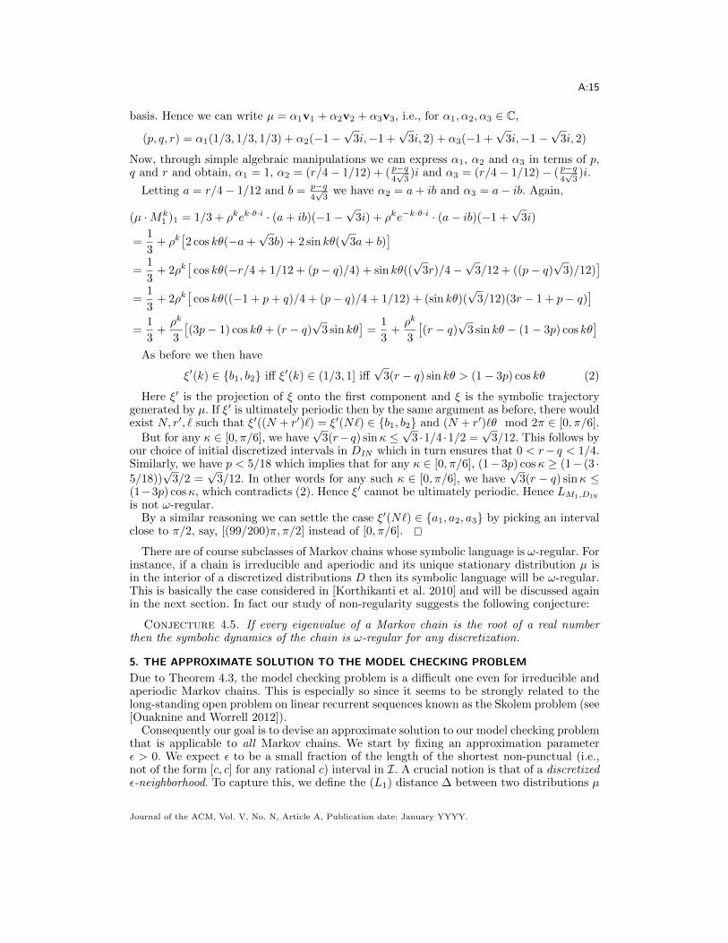
Proof. Consider M1 as above but fix a new discretization I = {a1 = [0, 1/4), a2 =[1/4, 5/18], a3 = (5/18, 1/3], b1 = (1/3, 1/2), b2 = [1/2, 1]}. Let DIN = (a2, a2, b1). Then,clearly DIN contains an infinite number of distributions. We will now show that no wordin LM1,DIN

is ultimately periodic which will establish the corollary.Let µ = (p, q, r) ∈ DIN . Then we have p ∈ [1/4, 5/18], q ∈ [1/4, 5/18] and r ∈ (1/3, 1/2).

From the proof of Theorem 4.3, we have that the eigenvectors v1,v2,v3 as before form a


A:15

basis. Hence we can write µ = α1v1 + α2v2 + α3v3, i.e., for α1, α2, α3 ∈ C,

(p, q, r) = α1(1/3, 1/3, 1/3) + α2(−1−√

3i,−1 +√

3i, 2) + α3(−1 +√

3i,−1−√

3i, 2)

Now, through simple algebraic manipulations we can express α1, α2 and α3 in terms of p,q and r and obtain, α1 = 1, α2 = (r/4− 1/12) + ( p−q

4√

3)i and α3 = (r/4− 1/12)− ( p−q

4√

3)i.

Letting a = r/4− 1/12 and b = p−q4√

3we have α2 = a+ ib and α3 = a− ib. Again,

(µ ·Mk1 )1 = 1/3 + ρkek·θ·i · (a+ ib)(−1−

√3i) + ρke−k·θ·i · (a− ib)(−1 +

√3i)

=1

3+ ρk

[2 cos kθ(−a+

√3b) + 2 sin kθ(

√3a+ b)

]=

1

3+ 2ρk

[cos kθ(−r/4 + 1/12 + (p− q)/4) + sin kθ((

√3r)/4−

√3/12 + ((p− q)

√3)/12)

]=

1

3+ 2ρk

[cos kθ((−1 + p+ q)/4 + (p− q)/4 + 1/12) + (sin kθ)(

√3/12)(3r − 1 + p− q)

]=

1

3+ρk

3

[(3p− 1) cos kθ + (r − q)

√3 sin kθ

]=

1

3+ρk

3

[(r − q)

√3 sin kθ − (1− 3p) cos kθ

]As before we then have

ξ′(k) ∈ {b1, b2} iff ξ′(k) ∈ (1/3, 1] iff√

3(r − q) sin kθ > (1− 3p) cos kθ (2)

Here ξ′ is the projection of ξ onto the first component and ξ is the symbolic trajectorygenerated by µ. If ξ′ is ultimately periodic then by the same argument as before, there wouldexist N, r′, ` such that ξ′((N + r′)`) = ξ′(N`) ∈ {b1, b2} and (N + r′)`θ mod 2π ∈ [0, π/6].

But for any κ ∈ [0, π/6], we have√

3(r−q) sinκ ≤√

3 ·1/4 ·1/2 =√

3/12. This follows byour choice of initial discretized intervals in DIN which in turn ensures that 0 < r− q < 1/4.Similarly, we have p < 5/18 which implies that for any κ ∈ [0, π/6], (1−3p) cosκ ≥ (1− (3 ·5/18))

√3/2 =

√3/12. In other words for any such κ ∈ [0, π/6], we have

√3(r − q) sinκ ≤

(1−3p) cosκ, which contradicts (2). Hence ξ′ cannot be ultimately periodic. Hence LM1,DIN

is not ω-regular.By a similar reasoning we can settle the case ξ′(N`) ∈ {a1, a2, a3} by picking an interval

close to π/2, say, [(99/200)π, π/2] instead of [0, π/6].

There are of course subclasses of Markov chains whose symbolic language is ω-regular. Forinstance, if a chain is irreducible and aperiodic and its unique stationary distribution µ isin the interior of a discretized distributions D then its symbolic language will be ω-regular.This is basically the case considered in [Korthikanti et al. 2010] and will be discussed againin the next section. In fact our study of non-regularity suggests the following conjecture:

Conjecture 4.5. If every eigenvalue of a Markov chain is the root of a real numberthen the symbolic dynamics of the chain is ω-regular for any discretization.

5. THE APPROXIMATE SOLUTION TO THE MODEL CHECKING PROBLEM

Due to Theorem 4.3, the model checking problem is a difficult one even for irreducible andaperiodic Markov chains. This is especially so since it seems to be strongly related to thelong-standing open problem on linear recurrent sequences known as the Skolem problem (see[Ouaknine and Worrell 2012]).

Consequently our goal is to devise an approximate solution to our model checking problemthat is applicable to all Markov chains. We start by fixing an approximation parameterε > 0. We expect ε to be a small fraction of the length of the shortest non-punctual (i.e.,not of the form [c, c] for any rational c) interval in I. A crucial notion is that of a discretizedε-neighborhood. To capture this, we define the (L1) distance ∆ between two distributions µ


A:16

and µ′ as: ∆(µ, µ′) =∑i |µ(i)−µ′(i)|. Clearly ∆ is a metric. The discretized ε-neighborhood

of µ is denoted as Nε(µ) and is the set of D-distributions given by:

D ∈ Nε(µ) iff there exists µ′ ∈ D such that ∆(µ, µ′) ≤ ε

We note that Nε(µ) is non-empty for every µ and ε since µ ∈ D implies D ∈ Nε.Finally F ⊆ D is a discretized ε-neighborhood iff there exists a distribution µ such that

Nε(µ) = F . For convenience, we will just say ε-neighborhood from now on.Suppose F is an ε-neighborhood and D1, D2 ∈ F . Then, by definition, there exists µ0

such that Nε(µ0) = F . Further there exist µ1 ∈ D1 and µ2 ∈ D2 such that ∆(µ1, µ0) ≤ εand ∆(µ2, µ0) ≤ ε. By the triangle inequality ∆(µ1, µ2) ≤ 2 · ε. In this sense, any twodiscretized distributions belonging to an ε-neighborhood will be close to each other.

5.1. The main verification results

The key to constructing an ε-approximate solution to our model checking problem is thefollowing insight. For any Markov chain M with discretization I and approximation factorε, every symbolic trajectory can be split into a transient and steady state phase. The lengthof the transient phase will depend only on M and ε and not on the initial distribution. Inthe steady state phase, the symbolic trajectory will simply cycle through a finite orderedfamily of ε-neighborhoods forever. The number of such neighborhoods will depend only onM. Consequently one can say that a symbolic trajectory ξ′ is an ε-approximation of thesymbolic trajectory ξ in case ξ′ agrees with ξ exactly during the transient phase while ξ′(k)and ξ(k) fall into the same ε-neighborhood for all k during the steady state phase. This willallow us to formulate our approximate solution to the model checking problem.

We now turn to a formalization of these ideas.

Proposition 5.1. Let M be a Markov chain, ε > 0 and ξµ the symbolic trajectorygenerated by the distribution µ. Then, there exists (i) a positive integer θ that dependsonly on M (ii) a positive integer Kε that depends only on M and ε and (iii) an orderedfamily of ε-neighborhoods {Fµ,0,Fµ,1, . . . ,Fµ,θ−1} - called the final classes of µ - such thatξµ(k) ∈ Fµ, k mod θ for every k > Kε. Further, θ, Kε and {Fµ,0,Fµ,1, . . . ,Fµ,θ−1} areeffectively computable.

The bulk of the technical work we carry out in the rest of the paper will be devoted toestablishing this result. We note that if Kε exists satisfying the requirements stated abovethen the result will also go through for any K > Kε. A basic component of the proof ofProp. 5.1 will consist of a deterministic algorithm to compute an adequate Kε. For now weassume Prop. 5.1 and and use it to define the notion of an ε-approximation of a symbolictrajectory.

Definition 5.2. Let µ be a distribution while θ, Kε and {Fµ,0,Fµ,1, . . . ,Fµ,θ−1} are asguaranteed by the above proposition. Then ξ′ ∈ Dω is an ε-approximation of ξµ iff thefollowing conditions hold:

— ξ′(k) = ξµ(k) for 0 ≤ k ≤ Kε.— For every k > Kε, ξ′(k) belongs to Fµ, k mod θ.

Clearly every ξµ is an ε-approximation of itself. We can formulate two closely relatedapproximate model checking problems as follows:

Definition 5.3. Let M be a Markov chain, DIN an initial distribution, ε > 0 an approx-imation factor and ϕ ∈ LTLI :

(1) (M,DIN ) ε-approximately meets the specification ϕ from below, denoted M,DIN |=ε ϕ,iff for every µ ∈ DIN , it is the case that ξ′ ∈ Lϕ for some ε-approximation ξ′ of ξµ.


A:17

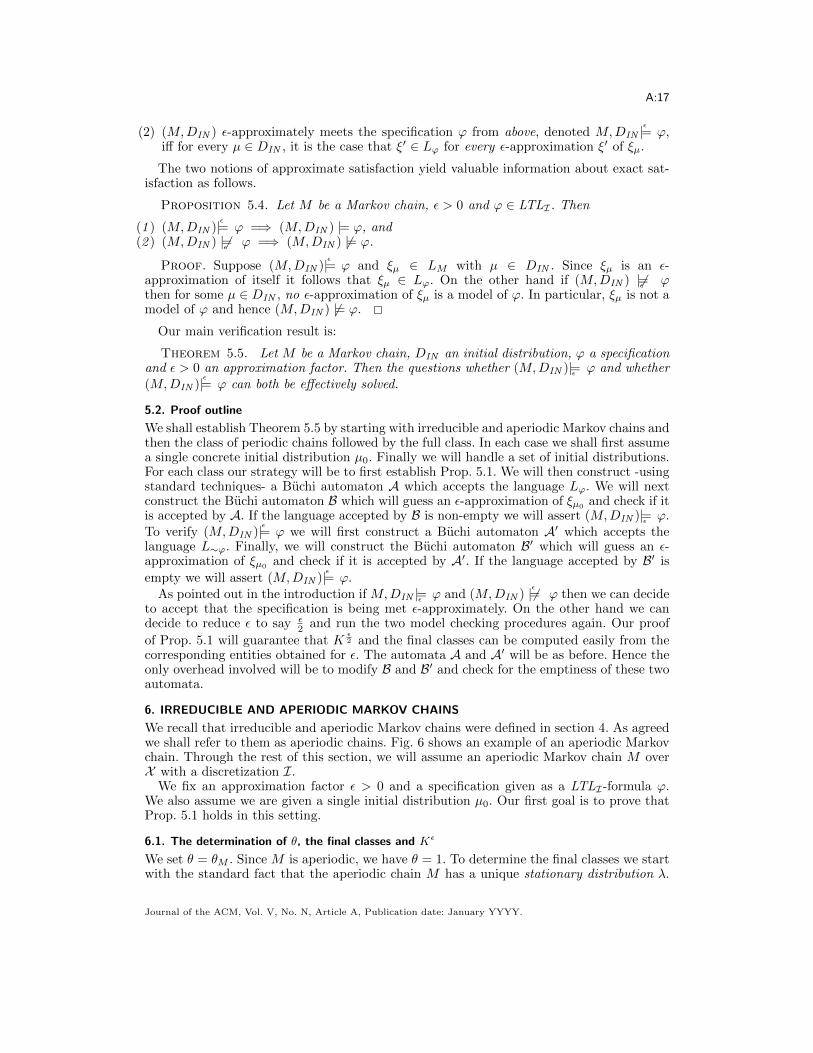
(2) (M,DIN ) ε-approximately meets the specification ϕ from above, denoted M,DIN |=ε

ϕ,iff for every µ ∈ DIN , it is the case that ξ′ ∈ Lϕ for every ε-approximation ξ′ of ξµ.

The two notions of approximate satisfaction yield valuable information about exact sat-isfaction as follows.

Proposition 5.4. Let M be a Markov chain, ε > 0 and ϕ ∈ LTLI . Then

(1 ) (M,DIN )|=ε ϕ =⇒ (M,DIN ) |= ϕ, and(2 ) (M,DIN ) 6|=

εϕ =⇒ (M,DIN ) 6|= ϕ.

Proof. Suppose (M,DIN )|=ε ϕ and ξµ ∈ LM with µ ∈ DIN . Since ξµ is an ε-approximation of itself it follows that ξµ ∈ Lϕ. On the other hand if (M,DIN ) 6|=ε ϕthen for some µ ∈ DIN , no ε-approximation of ξµ is a model of ϕ. In particular, ξµ is not amodel of ϕ and hence (M,DIN ) 6|= ϕ.

Our main verification result is:

Theorem 5.5. Let M be a Markov chain, DIN an initial distribution, ϕ a specificationand ε > 0 an approximation factor. Then the questions whether (M,DIN )|=

εϕ and whether

(M,DIN )|=ε ϕ can both be effectively solved.

5.2. Proof outline

We shall establish Theorem 5.5 by starting with irreducible and aperiodic Markov chains andthen the class of periodic chains followed by the full class. In each case we shall first assumea single concrete initial distribution µ0. Finally we will handle a set of initial distributions.For each class our strategy will be to first establish Prop. 5.1. We will then construct -usingstandard techniques- a Buchi automaton A which accepts the language Lϕ. We will nextconstruct the Buchi automaton B which will guess an ε-approximation of ξµ0

and check if itis accepted by A. If the language accepted by B is non-empty we will assert (M,DIN )|=

εϕ.

To verify (M,DIN )|=ε ϕ we will first construct a Buchi automaton A′ which accepts thelanguage L∼ϕ. Finally, we will construct the Buchi automaton B′ which will guess an ε-approximation of ξµ0 and check if it is accepted by A′. If the language accepted by B′ is

empty we will assert (M,DIN )|=ε ϕ.As pointed out in the introduction if M,DIN |=ε ϕ and (M,DIN ) 6|=ε ϕ then we can decide

to accept that the specification is being met ε-approximately. On the other hand we candecide to reduce ε to say ε

2 and run the two model checking procedures again. Our proof

of Prop. 5.1 will guarantee that Kε2 and the final classes can be computed easily from the

corresponding entities obtained for ε. The automata A and A′ will be as before. Hence theonly overhead involved will be to modify B and B′ and check for the emptiness of these twoautomata.

6. IRREDUCIBLE AND APERIODIC MARKOV CHAINS

We recall that irreducible and aperiodic Markov chains were defined in section 4. As agreedwe shall refer to them as aperiodic chains. Fig. 6 shows an example of an aperiodic Markovchain. Through the rest of this section, we will assume an aperiodic Markov chain M overX with a discretization I.

We fix an approximation factor ε > 0 and a specification given as a LTLI-formula ϕ.We also assume we are given a single initial distribution µ0. Our first goal is to prove thatProp. 5.1 holds in this setting.

6.1. The determination of θ, the final classes and Kε

We set θ = θM . Since M is aperiodic, we have θ = 1. To determine the final classes we startwith the standard fact that the aperiodic chain M has a unique stationary distribution λ.


A:18

1 2

25

710

35

310

Fixpoint= ( 711 ,

411 )

M =

35

25

710

310

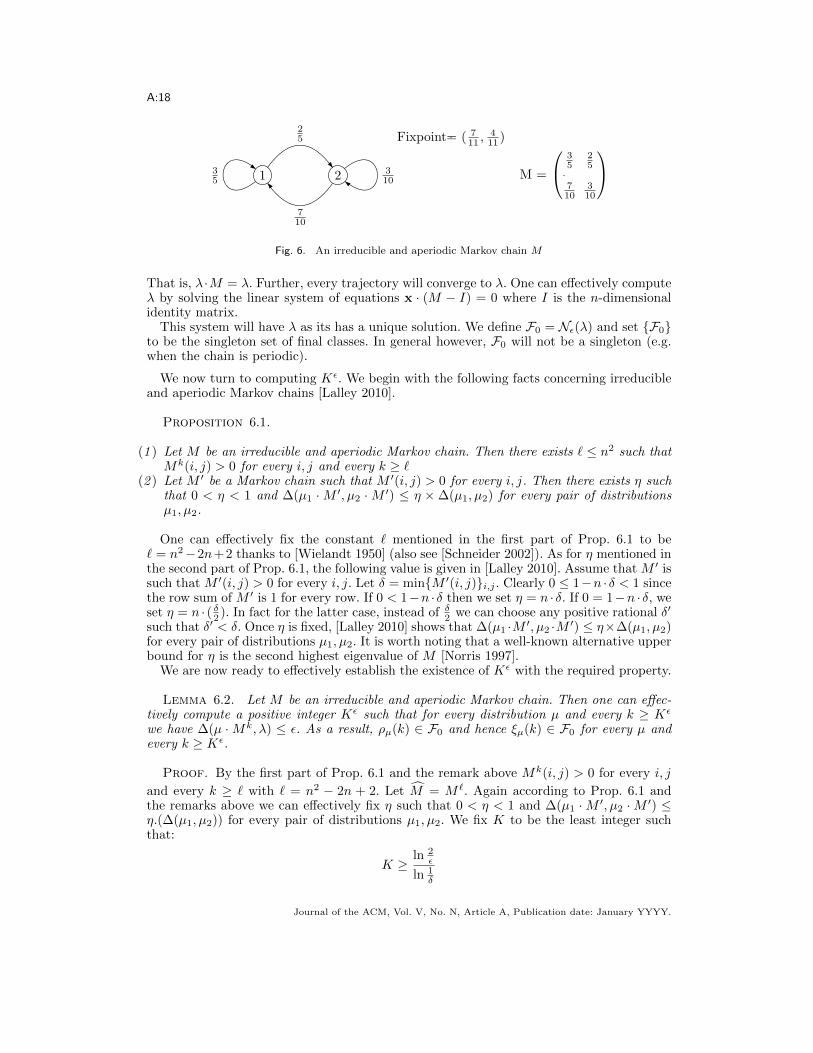
Fig. 6. An irreducible and aperiodic Markov chain M

That is, λ ·M = λ. Further, every trajectory will converge to λ. One can effectively computeλ by solving the linear system of equations x · (M − I) = 0 where I is the n-dimensionalidentity matrix.

This system will have λ as its has a unique solution. We define F0 = Nε(λ) and set {F0}to be the singleton set of final classes. In general however, F0 will not be a singleton (e.g.when the chain is periodic).

We now turn to computing Kε. We begin with the following facts concerning irreducibleand aperiodic Markov chains [Lalley 2010].

Proposition 6.1.

(1 ) Let M be an irreducible and aperiodic Markov chain. Then there exists ` ≤ n2 such thatMk(i, j) > 0 for every i, j and every k ≥ `

(2 ) Let M ′ be a Markov chain such that M ′(i, j) > 0 for every i, j. Then there exists η suchthat 0 < η < 1 and ∆(µ1 ·M ′, µ2 ·M ′) ≤ η × ∆(µ1, µ2) for every pair of distributionsµ1, µ2.

One can effectively fix the constant ` mentioned in the first part of Prop. 6.1 to be` = n2−2n+2 thanks to [Wielandt 1950] (also see [Schneider 2002]). As for η mentioned inthe second part of Prop. 6.1, the following value is given in [Lalley 2010]. Assume that M ′ issuch that M ′(i, j) > 0 for every i, j. Let δ = min{M ′(i, j)}i,j . Clearly 0 ≤ 1−n · δ < 1 sincethe row sum of M ′ is 1 for every row. If 0 < 1−n · δ then we set η = n · δ. If 0 = 1−n · δ, weset η = n · ( δ2 ). In fact for the latter case, instead of δ2 we can choose any positive rational δ′

such that δ′ < δ. Once η is fixed, [Lalley 2010] shows that ∆(µ1 ·M ′, µ2 ·M ′) ≤ η×∆(µ1, µ2)for every pair of distributions µ1, µ2. It is worth noting that a well-known alternative upperbound for η is the second highest eigenvalue of M [Norris 1997].

We are now ready to effectively establish the existence of Kε with the required property.

Lemma 6.2. Let M be an irreducible and aperiodic Markov chain. Then one can effec-tively compute a positive integer Kε such that for every distribution µ and every k ≥ Kε

we have ∆(µ ·Mk, λ) ≤ ε. As a result, ρµ(k) ∈ F0 and hence ξµ(k) ∈ F0 for every µ andevery k ≥ Kε.

Proof. By the first part of Prop. 6.1 and the remark above Mk(i, j) > 0 for every i, j

and every k ≥ ` with ` = n2 − 2n + 2. Let M = M `. Again according to Prop. 6.1 andthe remarks above we can effectively fix η such that 0 < η < 1 and ∆(µ1 ·M ′, µ2 ·M ′) ≤η.(∆(µ1, µ2)) for every pair of distributions µ1, µ2. We fix K to be the least integer suchthat:

K ≥ln 2

ε

ln 1δ


A:19

Then ηK · 2 ≤ ε. For any distribution µ we now have ∆(µ · Mk, λ · MK) = ∆(µ · MK , λ) ≤ηK ·∆(µ, λ) for every k ≥ K. But then ∆(µ, λ) ≤ 2 according to the definition of ∆. Hence

∆(µ · Mk, λ) ≤ ε for every µ and every k ≥ K.We now fix Kε = ` ·K. Consequently ∆(µ ·Mk, λ) ≤ ε for every µ and every k ≥ Kε.Since Nε(λ) = F0 we now have that ξµ(k) ∈ F0 for every µ and every k ≥ Kε as

required.

6.2. Solutions to the model checking problems

Recall that, in this section, we are assuming a single initial distribution µ0. To determinewhether (M,µ0)|=

εϕ we will construct a non-deterministic Buchi automaton B running over

sequences in Dω such that the language accepted by B is non-empty iff (M,µ0)|=εϕ. Since

the emptiness problem for Buchi automata is decidable, we will have an effective solutionto our model checking problem.

To start with, let Σ = 2APϕ with APϕ being the set of atomic propositions that appearin ϕ. Consider α ∈ Σω. As before, we will view α to be a map from {0, 1, 2, . . . } into Σ.The notion of α, k |=Σ ϕ is defined in the usual way:

— α, k |=Σ (i, d) iff (i, d) ∈ α(k).— The propositional connectives are interpreted in the standard way.— α, k |=Σ X(ϕ) iff α, k + 1 |=Σ ϕ.— α, k |=Σ ϕ1Uϕ2 iff there exists k′ ≥ k such that α, k′ |=Σ ϕ2 and α, k′′ |=Σ ϕ1 fork ≤ k′′ < k′.

We say that α is a Σ-model of ϕ iff α, 0 |=Σ ϕ. This leads to Lϕ = {α | α, 0 |= ϕ}.We next construct the non-deterministic Buchi automaton A = (Q,Qin,Σ,−→, A) run-

ning over infinite sequences in Σω such that the language accepted by A is exactly Lϕ. Thisis a standard construction [Vardi 1999] and here we shall recall just the basic details neededto establish Theorem 6.3 below.

We define CL(ϕ), (abbreviated as just CL) the (Fisher-Ladner) closure of ϕ to be theleast set of formulas containing ϕ and satisfying:

— ψ ∈ CL iff ¬ψ ∈ CL (with the convention ¬¬ψ is identified with ψ).— If ψ1 ∨ ψ2 ∈ CL then ψ1, ψ2 ∈ CL.— If X(ψ) ∈ CL then ψ ∈ CL.— If ψ1Uψ2 ∈ CL then ψ1, ψ2, X(ψ1Uψ2) ∈ CL.

We next define an atom to be a subset Z of CL satisfying the following conditions. Instating these conditions we assume the formulas mentioned are in CL.

— ψ ∈ Z iff ¬ψ /∈ Z.— ψ1 ∨ ψ2 ∈ Z iff ψ1 ∈ Z or ψ2 ∈ Z.— ψ1Uψ2 ∈ Z iff ψ2 ∈ Z or ψ1, X(ψ1Uψ2) ∈ Z.

Finally we define H = 2CLU where CLU is the until formulas contained in CL. This leadsto the Buchi automaton A = (Q,Qin,Σ,−→, A) given by:

—Q = AT ×H where AT is the set of atoms.— (Z,H) ∈ Qin iff ϕ ∈ Z. Further, ψ1Uψ2 ∈ H iff ψ1Uψ2 ∈ Z and ψ2 /∈ Z.—−→⊆ Q× Σ×Q is given by: ((Z1, H1), Y, (Z2, H2)) ∈−→ iff:

(1) (i, d) ∈ Y iff (i, d) ∈ Z1

(2)X(ψ) ∈ Z1 iff ψ ∈ Z2

(3) Suppose H1 is non-empty. Then ψ1Uψ2 ∈ H2 iff ψ1Uψ2 ∈ H1 and ψ2 /∈ Z2.(4) Suppose H1 = ∅. Then ψ1Uψ2 ∈ H2 iff ψ1Uψ2 ∈ Z2 and ψ2 /∈ Z2.

— (Z,H) ∈ A iff H = ∅


A:20

We can now define the Buchi automaton we seek. First let S = {(k, µ0 ·Mk) | 0 ≤ k ≤Kε}. Then our Buchi automaton is B = (R,Rin,Σ,⇒, B) defined via:

—R = (S ∪ F0)×Q is the set of states, where F0 = Nε(λ) as defined earlier.—Rin = {(0, µ0)} ×Qin is the set of initial states.— The transition relation⇒ is the least subset of R×Σ×R satisfying the following conditions

First, Suppose ((k, µ), q) and ((k′, µ′), q′) are in R and Y ⊆ APϕ. Then((k, µ), q), Y, (k′, µ′), q′)) ∈⇒ iff the following assertions hold:(1) k′ = k + 1 and µ ·M = µ′, and(2) Suppose (i, d) ∈ APϕ. Then µ(i) ∈ d iff (i, d) ∈ Y , and(3) (q, Y, q′) ∈−→.

Next, suppose ((k, µ), q)) and (D, q′) are in R with D ∈ F . Let Y ⊆ AP . Then((k, µ), q), Y, (D, q′) ∈⇒ iff k = Kε and (i, d) ∈ Y iff µ(i) ∈ d(i). Furthermore,(q, Y, q′) ∈−→.Finally, suppose (D, q) and (D′, q′) are in R and Y ⊆ APϕ. Then ((D, q), Y, (D′, q′)) ∈⇒iff for every (i, d) ∈ APϕ, D(i) = d iff (i, d) ∈ Y . Further, (q, Y, q′) ∈−→.

— The set of final states is B = F ×A.

We can now show:

Theorem 6.3. (M,µ0)|=ε ϕ iff the language accepted by B is non-empty.

Proof. Suppose (M,µ0)|=εϕ. Then there exists ξ′ such that ξ′ is an ε-approximation

of ξµ0and ξ′, 0 |= ϕ. For k ≥ 0, we set Zk = {ψ | ψ ∈ CL and ξ′, k |= ψ}. It is easy to

check that Zk is an atom for every k. Next we define {Hk} inductively via: ψ1Uψ2 ∈ H0

iff ψ1Uψ2 ∈ Z0 and ψ2 /∈ Z0. Next suppose Hk is defined. Then Hk+1 is given by: If Hk

is non-empty then ψ1Uψ2 ∈ Hk+1 iff ψ1Uψ2 ∈ Hk and ψ2 /∈ Zk+1. If Hk is empty thenψ1Uψ2 ∈ Hk+1 iff ψ1Uψ2 ∈ Hk+1 and ψ2 /∈ Zk+1.

We next define {sk}k≥0 via: For 0 ≤ k ≤ Kε, sk = µ0 ·Mk. And sk = ξ′(k) for k > Kε.Finally we define {Yk}k≥0 via: Yk = Zk ∩APϕ.

Let Υ : {0, 1, 2, . . .} → R via Υ(k) = (sk, (Zk, Hk)) for each k. It is now straightforwardto show that Υ is an accepting run of B over the infinite sequence α ∈ Σω with α(k) = Ykfor each k. Consequently the language accepted by B is non-empty as required.

Conversely, suppose the language accepted by B is non-empty. Then there exists α ∈ Σω

and an accepting run Υ : {0, 1, 2, . . .} → R of B over α. Let Υ(k) = ((sk, (Zk, Hk)) for eachk. We now define ξ′ as follows. (i) ξ′(k) = Γ(µk) for 0 ≤ k ≤ Kε where sk = (µk, k) for0 ≤ k ≤ Kε. (ii) ξ′(k) = sk for k > Kε. By structural induction on ψ we can now easilyshow that ξ′, k |= ψ iff ψ ∈ Zk for every k and every ψ ∈ CL. Since ϕ ∈ Z0 this willestablish that ξ′, 0 |= ϕ. By construction, ξ′ is an ε-approximation of ξµ0 . This completesthe proof.

To determine whether (M,µ0)|=ε ϕ, we first construct the non-deterministic Buchi au-tomaton A′ such that the language accepted by A′ is precisely L¬ϕ. We then repeat theabove construction using A′ in place of A to construct the automaton B′. It is then easy toshow that:

Theorem 6.4. M,µ0|=ε

ϕ iff the language accepted by B′ is empty.

Notice that transitions of B and B′ check whether the current distribution µ satisfies µ(i) ∈d, or D satisfies D(i) = d. Since the first order theory of reals is decidable, we can also decidewhether µ(i) or D(i) satisfies a sentence ψ in this theory. Hence our decision procedureseasily extend to the setting where atomic propositions consist of suitable sentences in thefirst order theory of reals (as discussed in Section 3).

We also note that if F0 itself is a singleton i.e. it consists of just one discretized distributionthen it is easy to show that the original model checking problem can be solved exactly. To


A:21

1

3 2

4

1

1

1

25

35

(a)

1 2

35

25

25

35

B0

3 41 1

B1 B2

(b)

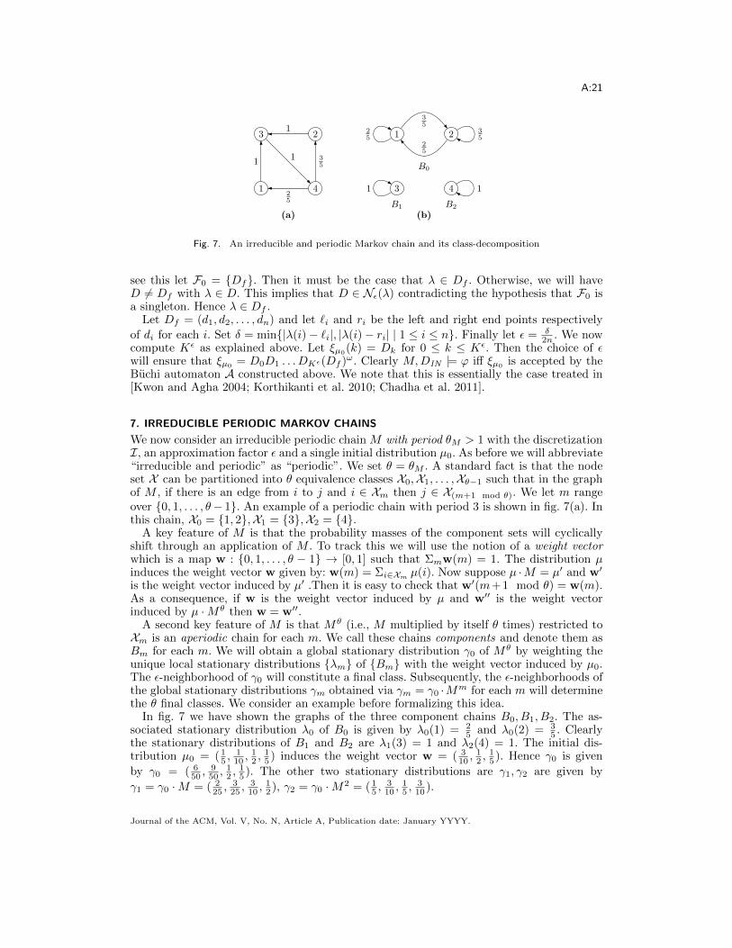
Fig. 7. An irreducible and periodic Markov chain and its class-decomposition

see this let F0 = {Df}. Then it must be the case that λ ∈ Df . Otherwise, we will haveD 6= Df with λ ∈ D. This implies that D ∈ Nε(λ) contradicting the hypothesis that F0 isa singleton. Hence λ ∈ Df .

Let Df = (d1, d2, . . . , dn) and let ì and ri be the left and right end points respectively

of di for each i. Set δ = min{|λ(i)− ì|, |λ(i)− ri| | 1 ≤ i ≤ n}. Finally let ε = δ2n . We now

compute Kε as explained above. Let ξµ0(k) = Dk for 0 ≤ k ≤ Kε. Then the choice of ε

will ensure that ξµ0= D0D1 . . . DKε(Df )ω. Clearly M,DIN |= ϕ iff ξµ0

is accepted by theBuchi automaton A constructed above. We note that this is essentially the case treated in[Kwon and Agha 2004; Korthikanti et al. 2010; Chadha et al. 2011].

7. IRREDUCIBLE PERIODIC MARKOV CHAINS

We now consider an irreducible periodic chain M with period θM > 1 with the discretizationI, an approximation factor ε and a single initial distribution µ0. As before we will abbreviate“irreducible and periodic” as “periodic”. We set θ = θM . A standard fact is that the nodeset X can be partitioned into θ equivalence classes X0,X1, . . . ,Xθ−1 such that in the graphof M , if there is an edge from i to j and i ∈ Xm then j ∈ X(m+1 mod θ). We let m rangeover {0, 1, . . . , θ− 1}. An example of a periodic chain with period 3 is shown in fig. 7(a). Inthis chain, X0 = {1, 2},X1 = {3},X2 = {4}.

A key feature of M is that the probability masses of the component sets will cyclicallyshift through an application of M . To track this we will use the notion of a weight vectorwhich is a map w : {0, 1, . . . , θ − 1} → [0, 1] such that Σmw(m) = 1. The distribution µinduces the weight vector w given by: w(m) = Σi∈Xm µ(i). Now suppose µ ·M = µ′ and w′

is the weight vector induced by µ′ .Then it is easy to check that w′(m+1 mod θ) = w(m).As a consequence, if w is the weight vector induced by µ and w′′ is the weight vectorinduced by µ ·Mθ then w = w′′.

A second key feature of M is that Mθ (i.e., M multiplied by itself θ times) restricted toXm is an aperiodic chain for each m. We call these chains components and denote them asBm for each m. We will obtain a global stationary distribution γ0 of Mθ by weighting theunique local stationary distributions {λm} of {Bm} with the weight vector induced by µ0.The ε-neighborhood of γ0 will constitute a final class. Subsequently, the ε-neighborhoods ofthe global stationary distributions γm obtained via γm = γ0 ·Mm for each m will determinethe θ final classes. We consider an example before formalizing this idea.

In fig. 7 we have shown the graphs of the three component chains B0, B1, B2. The as-sociated stationary distribution λ0 of B0 is given by λ0(1) = 2

5 and λ0(2) = 35 . Clearly

the stationary distributions of B1 and B2 are λ1(3) = 1 and λ2(4) = 1. The initial dis-tribution µ0 = ( 1

5 ,110 ,

12 ,

15 ) induces the weight vector w = ( 3

10 ,12 ,

15 ). Hence γ0 is given

by γ0 = ( 650 ,

950 ,

12 ,

15 ). The other two stationary distributions are γ1, γ2 are given by

γ1 = γ0 ·M = ( 225 ,

325 ,

310 ,

12 ), γ2 = γ0 ·M2 = ( 1

5 ,310 ,

15 ,

310 ).


A:22

7.1. The determination of Kε and the final classes

As fixed above, let θ = θM be the period of M . In constructing the final classes and Kε thebasic observation is that the infinite sequence of distributions (µ0·Mk)k≥0 can be analyzed in

terms of the θ subsequences (µm ·Mθ·k′)k′≥0 where µm = µ0 ·Mm for 0 ≤ m ≤ θ−1. Actually

one just needs to consider the first subsequence (µ0 ·Mθ·k′)k′≥0. The other subsequencescan be simply obtained by applying Mm (0 < m < θ) to each element of this subsequence.

Before proceeding it will be convenient to introduce some additional notations using whichwe can analyze the global behavior of Mθ in terms of the local behaviors of the components{Bm}. Let w be the weight vector induced by the distribution µ. Then ↓m (µ) = β is the

map β : Xm → [0, 1] given by: β(i) = µ(i)w(m) if w(m) 6= 0 and β(i) = 0 if w(m) = 0. It is

easy to see that β is a distribution over Xm in case w(m) 6= 0.Next let {βm} be such that for each m, either βm is a distribution over Xm or βm = 0m

(where 0m(i) = 0 for each i ∈ Xm). Suppose w is a weight vector. Then ↑w {βm} is themap µ : X → [0, 1] given by µ(i) = w(m) · βm(i) if i ∈ Xm. In the contexts in which we usethis map, it will turn out that µ is a distribution over X . In particular, if w is induced byµ then ↑w {↓m (µ)} = µ.

We are now prepared to define the final classes. Let λm be the unique stationary distri-bution of the component Bm for each m. Let u be the weight vector induced by µ0. Wenow define γ0 =↑u {λm}. It is not difficult to check that γ0 is a stationary distribution ofMθ. For each m < θ, we let γm = γ0 ·Mm. Finally, we define {Fm = Nε(γm)}0≤m<θ as theset of final classes.

To determine Kε we note that due to Lemma 6.2, for each component Bm we can ef-fectively determine an integer Kε,m such that for any distribution ν over Xm (in Bm),

∆(λm, ν ·BKε,mm ) ≤ ε. We now set Kε = θ ·maxm{Kε,m}.

To show that Kε has the required properties we begin with:

Lemma 7.1. Suppose µ is a distribution and w is the weight vector induced by µ. Letd ≥ 0 and µ ·Mθ·d = µ′. Then µ′ =↑w {Bdm(↓m (µ))}.

The proof follows easily from the definitions.

Lemma 7.2. ξµ0(k) ∈ F(k mod θ) for every k > Kε.

Proof. Let µ0 ·Mk = µ′ with k > Kε. We shall show that ∆(µ′, γ(k mod θ)) ≤ Kε. Thiswill imply that ξµ0

(k) ∈ F(k mod θ) as required.Let us consider first the case k mod θ = 0 with k′ = k · θ. Let ↓m (µ0) = βm for each m

and assume u is the weight vector induced by µ0. Set βm · Bk′

m = β′m for each m. For eachm, in case u(m) = 0, we have βm = 0m and hence β′m = 0m. In case u(m) > 0, by thechoice of Kε we are guaranteed ∆(β′m, λm) ≤ ε.

According to the previous lemma µ′ =↑u {β′m}. Hence ∆(µ′, γ0) = Σm cm where cm =Σi∈Xm |u(m) · β′m(i)− u(m) · λm| ≤ u(m) · ε. Since Σmu(m) = 1 we now have ∆(µ′, γ0) ≤ εas required. The other cases for k = k′θ + m for 0 < m < θ follow easily from: ∆(µ0 ·Mk, γm) = ∆(µ0 · Mk′θ · Mm, γ0 · Mm) ≤ ∆(µ0 · Mk′θ, γ0) ≤ ε, due to the fact that∆(µ ·M,µ′ ·M) ≤ ∆(µ, µ′) for any Markov chain M .

We have now established Prop. 5.1 for the class of periodic Markov chains.

7.2. Solutions to the approximate model checking problems

We next turn to the construction of a Buchi automaton B such that the language acceptedby this automaton B is non-empty if and only if M,µ0|=ε ϕ. As before, we let Σ = 2APϕ

and first construct the non-deterministic Buchi automaton A = (Q,Qin,Σ,−→, A) running


A:23

over infinite sequences in Σω such that LA, the language accepted by A is exactly Lϕ, theset of Σ-models of ϕ.

We let S = {(k, µ0 ·Mk) | 0 ≤ k ≤ Kε}. In addition, let F =⋃m Fm. The required

Buchi automaton B can now be constructed along the lines followed in the previous section.Intuitively, starting from µ0, B will iteratively apply M and simulate A on the resultingD-distributions. At the end of Kε steps the resulting discretized distribution is guaranteedto be in F0. Starting from here, if the current D-distribution is in Fm then the automatonwill non-deterministically move to a D-distribution in Fm+1 mod θ in the next step whilecontinuing to simulate the automaton A on the resulting D-distributions. The resulting runis accepted if A reports success. Otherwise it is rejected.

Formally, we define the Buchi automaton B = (R,Rin,Σ,=⇒, B) by:

—R = (S ∪ F )×Q is the set of states.—Rin = {(0, µ0)} ×Qin is the set of initial states.— The transition relation =⇒ is the least subset of R × Σ × R satisfying the following

conditions.Suppose ((k, µ), q) and ((k′, µ′), q′) are in R and Y ⊆ APϕ. Then((k, µ), q), Y, (k′, µ′), q′)) ∈=⇒ iff the following assertions hold:(1) k′ = k + 1 and µ ·M = µ′

(2) Suppose (i, d) ∈ APϕ. Then (i, d) ∈ Y iff µ(i) ∈ d(3) (q, Y, q′) ∈−→

Next suppose ((k, µ), q) and (D, q′) are in R with D ∈ F . Let Y ⊆ APϕ. Then((k, µ), q), Y, (D, q′) ∈=⇒ iff k = Kε and (i, d) ∈ Y iff µ(i) ∈ d(i) for every (i, d) ∈ AP .Furthermore, D ∈ Fµ0,1 and (q, Y, q′) ∈−→.Finally suppose (D, q) and (D′, q′) are in R and Y ⊆ APϕ. Then (D, q), Y, (D′, q′) ∈=⇒iff (q, Y, q′) ∈−→ and D ∈ Fµ0,m implies D′ ∈ Fµ0,m+1 mod θ. Moreover, (i, d) ∈ D iff(i, d) ∈ Y for every (i, d) ∈ APϕ

—B = F ×A.

By mildly modifying the arguments used to prove Theorem 6.3, we can now easily prove:

Theorem 7.3. M,µ0|=ε ϕ iff the language accepted by B is non-empty.

To determine whether M,µ0|=ε

ϕ we first construct the automaton A′ which accepts L¬ϕ.We then use it instead of the automaton A to construct a Buchi automaton B′ such thatM,µ0|=

ε


8. UNRESTRICTED MARKOV CHAINS

Let M be a Markov chain with the discretization I, an approximation factor ε and an initialdistribution µ0. We shall assume without loss of generality that for every node i if µ0(i) = 0then there exists a node j such that µ0(j) > 0 and there is a directed path from j to i.We can ensure this by removing all the nodes which don’t satisfy this condition and theiroutgoing edges.

In order to analyze general Markov chains, we will use the standard technique of de-composing them into strongly and bottom strongly connected components (see [Baier andKatoen 2008] for details). Y ⊆ X is a strongly connected component of M iff (i) there isa directed path of length ≥ 0 from i to j for every i, j in Y and (ii) if Y ⊆ Y ′ and Y ′ is astrongly connected component then Y = Y ′. Let {SC1, SC2, . . . , SCr} be the set of stronglyconnected components (SCCs) of GM . The relation � over the SCCs is given by: SC � SC ′iff there exists a node i in SC, a node j in SC ′ and a path from i to j in GM . Clearly �is a partial ordering relation and the maximal elements under � will be called the bottomstrongly connected components (BCCs). M restricted to a BCC is a Markov chain, and this


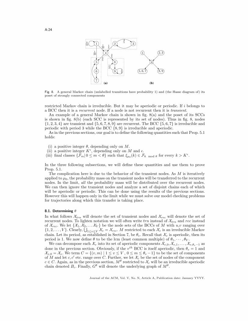
A:24

1 2 3

4

5

6

7

8

9

1

20

1

20

1

5

3

5

2

5

4

5

1

2

1

2

9

10

(a) (b)

1 2, 3

4

5, 6, 7 8, 9

Fig. 8. A general Markov chain (unlabelled transitions have probability 1) and (the Hasse diagram of) itsposet of strongly connected components

restricted Markov chain is irreducible. But it may be aperiodic or periodic. If i belongs toa BCC then it is a recurrent node. If a node is not recurrent then it is transient.

An example of a general Markov chain is shown in fig. 8(a) and the poset of its SCCsis shown in fig. 8(b) (each SCC is represented by its set of nodes). Thus in fig. 8, nodes{1, 2, 3, 4} are transient and {5, 6, 7, 8, 9} are recurrent. The BCC {5, 6, 7} is irreducible andperiodic with period 3 while the BCC {8, 9} is irreducible and aperiodic.

As in the previous sections, our goal is to define the following quantities such that Prop. 5.1holds:

(i) a positive integer θ, depending only on M .(ii) a positive integer Kε, depending only on M and ε.(iii) final classes {Fm| 0 ≤ m < θ} such that ξµ0(k) ∈ Fk mod θ for every k > Kε.

In the three following subsections, we will define these quantities and use them to proveProp. 5.1.

The complication here is due to the behavior of the transient nodes. As M is iterativelyapplied to µ0, the probability mass on the transient nodes will be transferred to the recurrentnodes. In the limit, all the probability mass will be distributed over the recurrent nodes.We can then ignore the transient nodes and analyze a set of disjoint chains each of whichwill be aperiodic or periodic. This can be done using the results of the previous sections.However this will happen only in the limit while we must solve our model checking problemsfor trajectories along which this transfer is taking place.

8.1. Determining θ

In what follows Xtrn will denote the set of transient nodes and Xrec will denote the set ofrecurrent nodes. To lighten notation we will often write trn instead of Xtrn and rec insteadof Xrec. We let {X1,X2, . . .XV } be the node sets of the BCCs of M with u,v ranging over{1, 2, . . . , V }. Clearly,

⋃1≤v≤V Xv = Xrec. M restricted to each Xv is an irreducible Markov

chain. Let its period, as established in Section 7, be θv. Recall that Xv is aperiodic, then itsperiod is 1. We now define θ to be the lcm (least common multiple) of θ1, · · · , θV .

We can decompose each Xv into its set of aperiodic components Xv,0,Xv,1, . . . ,Xv,θv−1 asdone in the previous section. Obviously, if the vth BCC is itself aperiodic, then θv = 1 andXv,0 = Xv. We term C = {(v,m) | 1 ≤ v ≤ V , 0 ≤ m ≤ θv−1} to be the set of componentsof M and let c, c′ etc. range over C. Further, we let Xc be the set of nodes of the componentc ∈ C. Again, as in the previous section, Mθ restricted to Xc will be an irreducible aperiodicchain denoted Bc. Finally, Gθ will denote the underlying graph of Mθ.


A:25

8.2. Determining the final classes

Let λc be the unique stationary distribution of Bc for each component c. A key entity thatwe wish to compute is a weight vector w : C → [0, 1] such that w(c) is the probability masstransferred to Xc in the limit. This will lead to the stationary distribution γ0 given by γ0 =∑cw(c)λc. As we shall argue below w(c) will turn out to be the limit of

∑j∈Xc(µ0 ·Mkθ)(j)

as k tends to infinity. In what follows, for the probability distribution µ we let µ(Xc) denote∑j∈Xc µ(j).

8.2.1. Computing the weight vector (the net probability mass transferred to Xc via Mθ in the limit).First we define πi to be the distribution given by πi(j) = 1 if j = i and πi(j) = 0 otherwise.Clearly µ0 can be expressed uniquely as a linear combination of the distributions (viewedas n-dimensional vectors) {π1, π2, . . . , πn}. Hence for the sake of convenience we will oftenwork with the distributions πi instead of µ0 and then use linearity to generalize. We arethus interested in the quantity (πi ·Mkθ)(Xc) for all i, c, k.

We compute w(c) by solving a system of linear equations using the machinery developedin [Baier and Katoen 2008]. Specifically, given the component c, we partition the set ofnodes X into three subsets S0

c , S1c and S?

c as follows. In doing so by a “path” we shall meana directed path in Gθ:

— S0c = {j ∈ X | there does not exist a path from j to any node in Xc in Gθ}.

— S1c = Xc.

— S?c ⊆ trn is the set of transient nodes from each of which there is a path to a node of Xc.

It is easy to check that {S0c , S

1c , S

?c} is indeed a partition of X . That is, S?

c = X−(S0c ∪S1

c ).Further, we observe that each i ∈ S0

c , we have (πi ·Mkθ)(Xc) = 0 for all k ∈ N. Moreover,for each i ∈ S1

c , we have (πi ·Mkθ)(Xc) = 1 for all k ∈ N. This follows easily by inductionon k since c is a BCC. It remains to compute (πi ·Mkθ)(Xc) for i ∈ S?

c and all k ∈ N.Now let Ac be the matrix Mθ restricted to S?

c ×S?c , and bc(i) =

∑j∈XcM

θ(i, j) for each

i in S?c . To capture the iterative transfer of probability mass from the transient nodes to

(the nodes in) c, we define a set of vectors {x(k)c } via:

x(0)c = 0 (where 0(i) = 0 for every i in S?

c ) and x(k+1)c = Acx

(k)c + bc

We now wish to prove some properties of x(k)c . First, notice that unfolding the recursive

definition of x(k)c , we get x

(k+1)c (i) = bc(i) +

∑1≤j≤k(Ajc ·bc)(i) for each i in S?

c and for all

k. We let µ denote the restriction of µ to S?c . We then have:

Lemma 8.1.

(1 ) Let c ∈ C, and i ∈ S?c and k ∈ N. Then x

(k)c (i) = (πi ·Mkθ)(Xc).

(2 ) Let µ be a distribution. Then (µ ·Mkθ)(Xc) = µ(Xc) + µ · x(k)c .

Proof. We will prove (1) by induction on k.

The case k = 1 is easy since x(1)c (i) = bc(i) = (

∑j∈XcM

θ)(i, j)) = (πi ·Mθ)(Xc)Now, assume (1) holds for k. Let ν = πi ·Mk·θ. We express ν as ν = ν0 + ν1 + ν?, where

ν0(j) = ν(j) for j ∈ S0c , ν0(j) = 0 else; ν1(j) = ν(j) for j ∈ S1

c , ν1(j) = 0 else; ν?(j) = ν(j)

for j ∈ S?c , ν?(j) = 0 else. By the induction hypothesis x

(k)c (i) = (πi ·Mkθ)(Xc) = ν(Xc) =

ν1(Xc). We thus get x(k+1)c (i) = ν1(Xc) + (Akc · bc)(i) (see the unrolling of the definition of

x(k+1)c (i) above).We have that (πi·M (k+1)θ)(Xc) = (ν·Mθ)(Xc) = (ν1Mθ)(Xc)+(ν0Mθ)(Xc)+(ν?Mθ)(Xc).

By the definition of S0c and S1

c , with k = 1, we immediately get (ν1 ·Mθ)(Xc) = ν1(Xc), andthat (ν0 ·Mθ)(Xc) = 0. Now, we notice that (ν?Mθ)(Xc) =

∑j∈Xc

∑k∈S?

cν?(k) ·M(k, j).


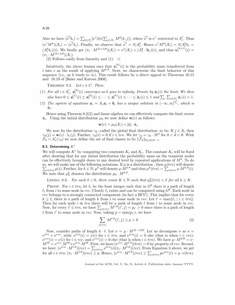
A:26

Also we have (ν?bc) =∑k∈S?

c[ν?(k)(

∑j∈XcM

θ(k, j)], where ν? is ν? restricted to S?c . Thus

(ν?Mθ)(Xc) = (ν?bc). Finally, we observe that ν? = πiAkc . Hence ν?Mθ(Xc) = πiA

kc bc =

(Akc bc)(i). We finally get (πi ·M (k+1)θ)(Xc) = ν1(Xc) + (Akc · bc)(i), and thus x(k+1)c (i) =

(πi ·M (k+1)θ)(Xc).(2) Follows easily from linearity and (1).

Intuitively, the above lemma says that x(k)c (i) is the probability mass transferred from

i into c as the result of applying Mk·θ. Next, we characterize the limit behavior of thissequence (i.e., as k tends to ∞). This result follows by a direct appeal to Theorems 10.15and 10.19 of [Baier and Katoen 2008].

Theorem 8.2. Let c ∈ C. Then:

(1 ) For all i ∈ S?c , x

(k)c (i) converges as k goes to infinity. Denote by xc(i) the limit. We then

also have 0 ≤ x(1)c (i) ≤ x

(2)c (i) ≤ · · · ≤ x

(k)c (i) ≤ · · · ≤ xc(i) ≤ 1 and

∑c

∑i∈S?

cxc(i) = 1.

(2 ) The system of equations xc = Acxc + bc has a unique solution in [−∞,∞]S?c , which is

xc.

Hence using Theorem 8.2(2) and linear algebra we can effectively compute the limit vectorxc. Using the initial distribution µ0 we now define w(c) as follows:

w(c) = µ0(Xc) + µ0 · xcWe now fix the distribution γ0 -called the global final distribution- to be: If j ∈ Xc then

γ0(j) = w(c) · λc(j). Further, γ0(i) = 0 if i ∈ trn. We let γd = γ0 ·Md for 0 < d < θ. WithFd = Nε(γd) we now define the set of final classes to be {Fd}0≤d≤θ−1.

8.3. Determining Kε

We will compute Kε by computing two constants Kt and Kr. The constant Kt will be fixedafter showing that for any initial distribution the probability mass on the transient nodescan be effectively brought down to any desired level by repeated applications of Mθ. To doso, we will make use of the following notations. If µ is a distribution , then µ(trn) will denote∑i∈trn µ(i). Further, for k ∈ N, µk will denote µ·Mk·θ and thus µk(trn) =

∑i∈trn µ·Mk·θ(i).

We note that µk0 denotes the distribution µ0 ·Mk·θ.

Lemma 8.3. For each δ > 0, there exists K ∈ N such that µk0(trn) < δ for all k ≥ K.

Proof. For i ∈ trn, let ì be the least integer such that in Gθ there is a path of lengthì from i to some node in rec. Clearly ì exists and can be computed using Gθ. Each node inrec belongs to a strongly connected component (in fact a BCC). This implies that for everyk ≥ li there is a path of length k from i to some node in rec. Let ` = max{ì | i ∈ trn}.Then for each node i in trn there will be a path of length ` from i to some node in rec.Now, for every i′ ∈ trn, we have

∑j∈recM

`·θ(i′, j) = pi′ > 0 since there is a path of length

` from i′ to some node in rec. Now, taking p = min(pi′), we have∑j∈rec

M `·θ(i′, j) ≥ p > 0 (3)

Now, consider paths of length k · `. Let ν = µ ·M (k−1)`θ. Let us decompose ν as ν =νtrn + νrec, with: νtrn(i) = ν(i) for i ∈ trn, and νtrn(i) = 0 else (that is when i ∈ rec).νrec(i) = ν(i) for i ∈ rec, and νrec(i) = 0 else (that is when i ∈ trn). We have µ ·Mk`θ = ν ·M `θ = νrec ·M `θ+νtrn ·M `θ. First, we have (νrec ·M `·θ)(trn) = 0 by property of rec. Second,we have: (νtrn ·M `·θ)(rec) =

∑i∈trn ν

trn(i)(πi ·M `·θ)(rec). From Equation 3 above, we get

for all i ∈ trn: (πi ·M `·θ)(rec) ≥ p. Hence, (νtrn ·M `·θ)(rec) ≥∑i∈trn pν

trn(i) = p · ν(trn).


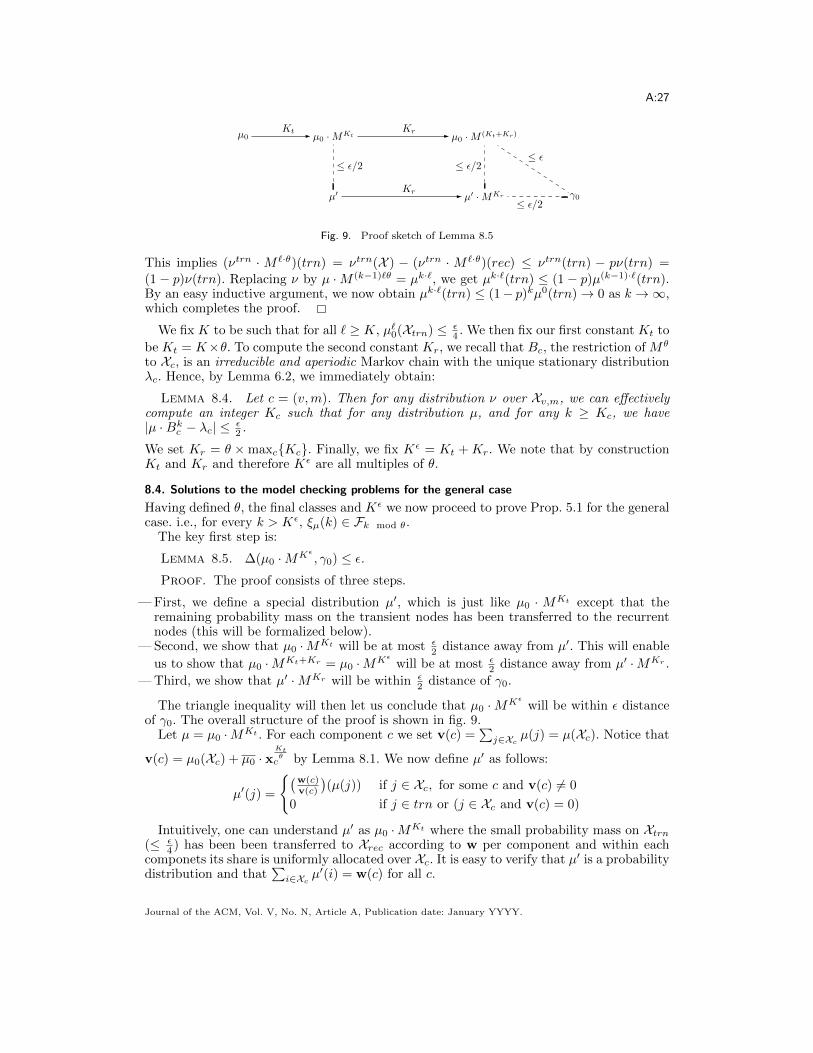
A:27

µ0 µ0 ·MKt µ0 ·M

(Kt+Kr)

µ′ µ′ ·MKr γ0

Kt Kr

Kr

≤ ǫ/2 ≤ ǫ/2

≤ ǫ/2

≤ ǫ

Fig. 9. Proof sketch of Lemma 8.5

This implies (νtrn · M `·θ)(trn) = νtrn(X ) − (νtrn · M `·θ)(rec) ≤ νtrn(trn) − pν(trn) =(1− p)ν(trn). Replacing ν by µ ·M (k−1)`θ = µk·`, we get µk·`(trn) ≤ (1− p)µ(k−1)·`(trn).By an easy inductive argument, we now obtain µk·`(trn) ≤ (1− p)kµ0(trn)→ 0 as k →∞,which completes the proof.

We fix K to be such that for all ` ≥ K, µ`0(Xtrn) ≤ ε4 . We then fix our first constant Kt to

be Kt = K×θ. To compute the second constant Kr, we recall that Bc, the restriction of Mθ

to Xc, is an irreducible and aperiodic Markov chain with the unique stationary distributionλc. Hence, by Lemma 6.2, we immediately obtain:

Lemma 8.4. Let c = (v,m). Then for any distribution ν over Xv,m, we can effectivelycompute an integer Kc such that for any distribution µ, and for any k ≥ Kc, we have|µ ·Bkc − λc| ≤ ε

2 .

We set Kr = θ ×maxc{Kc}. Finally, we fix Kε = Kt + Kr. We note that by constructionKt and Kr and therefore Kε are all multiples of θ.

8.4. Solutions to the model checking problems for the general case

Having defined θ, the final classes and Kε we now proceed to prove Prop. 5.1 for the generalcase. i.e., for every k > Kε, ξµ(k) ∈ Fk mod θ.

The key first step is:

Lemma 8.5. ∆(µ0 ·MKε

, γ0) ≤ ε.Proof. The proof consists of three steps.

— First, we define a special distribution µ′, which is just like µ0 · MKt except that theremaining probability mass on the transient nodes has been transferred to the recurrentnodes (this will be formalized below).

— Second, we show that µ0 ·MKt will be at most ε2 distance away from µ′. This will enable

us to show that µ0 ·MKt+Kr = µ0 ·MKε

will be at most ε2 distance away from µ′ ·MKr .

— Third, we show that µ′ ·MKr will be within ε2 distance of γ0.

The triangle inequality will then let us conclude that µ0 ·MKε

will be within ε distanceof γ0. The overall structure of the proof is shown in fig. 9.

Let µ = µ0 ·MKt . For each component c we set v(c) =∑j∈Xc µ(j) = µ(Xc). Notice that

v(c) = µ0(Xc) + µ0 · xKtθc by Lemma 8.1. We now define µ′ as follows:

µ′(j) =

{(w(c)v(c)

)(µ(j)) if j ∈ Xc, for some c and v(c) 6= 0

0 if j ∈ trn or (j ∈ Xc and v(c) = 0)

Intuitively, one can understand µ′ as µ0 ·MKt where the small probability mass on Xtrn(≤ ε

4 ) has been been transferred to Xrec according to w per component and within eachcomponets its share is uniformly allocated over Xc. It is easy to verify that µ′ is a probabilitydistribution and that

∑i∈Xc µ

′(i) = w(c) for all c.


A:28

First we wish to establish:

Claim 1. ∆(µ′, µ) ≤ ε2 .

Proof of claim. We have ∆(µ′, µ) =∑i∈trn |µ′(i)− µ(i)|+

∑j∈rec |µ′(j)− µ(j)|. We

have µ′(i) = 0 for i ∈ trn. Further µ = µ0 ·MKt . Hence from the choice of Kt, we have:∑i∈trn

|µ′(i)− µ(i)| =∑i∈trn

µ(i) ≤ ε

4(4)

We now wish to argue that∑j∈rec |µ′(j) − µ(j)| ≤ ε

4 as well. First we shall show that

µ′(j) ≥ µ(j) for every j ∈ rec. First consider the case v(c) = 0. Then µ(j) = 0 and wehave µ′(j) = 0 too which implies µ′(j) ≥ µ(j). Now suppose v(c) > 0. We have v(c) =

µ0(Xc)+µ0 ·xKt/θc by Lemma 8.1. Also, we have by definition w(c) = µ0(Xc)+µ0 · xc. Now,

x(k)c (j) ≤ xc(j) for all j and all k (Theorem 8.2(1)). Hence w(c) ≥ v(c) and consequentlyµ′(j) ≥ µ(j) for every j ∈ Xc.

Hence,∑j∈rec |µ′(j) − µ(j)| =

∑j∈rec(µ

′(j) − µ(j)). Clearly∑j∈rec(µ

′(j) − µ(j)) =∑c∈C

∑j∈Xc(µ

′(j)− µ(j)).

Now we note that∑j∈Xc(µ

′(j) − µ(j)) =∑j∈Xc µ(j) · (w(c)

v(c) − 1) =∑j∈Xc

w(c)−v(c)v(c) (µ(j)) = w(c)−v(c)

v(c)

∑j∈Xc µ(j) = w(c)− v(c). Thus, we have:

∑j∈rec

|µ′(j)− µ(j)| =∑c∈C

∑j∈Xc

|µ′(j)− µ(j)| =∑c∈C

(w(c)− v(c)) (5)

Next we wish to argue that∑c∈C w(c) = 1. We have

∑c∈C w(c) =

∑c∈C µ0(Xc) +∑

c∈C µ0 · xc = µ0(rec) +∑c∈C

∑i∈S?

cµ0(i)xc(i) Now, for all c, extending xc from S?

c to

trn by setting xc(i) = 0 for i ∈ trn \ S?c , we get

∑i∈S?

cµ0(i)xc(i) =

∑i∈trn µ0(i)xc(i).

Thus∑c∈C

∑i∈S?

cµ0(i)xc(i) =

∑i∈trn µ0(i)

∑c∈C xc(i). Now, as

∑c∈C xc(i) = 1 for all i

by theorem 8.2(1), we get∑c∈C w(c) = µ0(rec) +

∑i∈trn µ0(i) = µ0(rec) + µ0(trn) = 1 as

µ0 is a distribution.Next we note that

∑c∈C v(c) =

∑c∈C

∑j∈Xc µ(j) =

∑j∈rec µ(j) = 1−

∑i∈trn µ(i). We

now have∑c∈C(w(c)−v(c)) = 1− (1−

∑i∈trn(µ(i))) =

∑i∈trn µ(i). Due to the equations

(4) and (5) above, we now obtain ∆(µ′, µ) ≤ ε2 . [end of claim]

Now, for any pair of distributions ν, ν′ we have ∆(ν′ · M,ν · M) ≤ ∆(ν′, ν). Hence∆(µ′ ·MKr , µ ·MKr ) ≤ ∆(µ′, µ) ≤ ε

2 . Hence ∆(µ′ ·MKr , µ0 ·MKε

) ≤ ε2 .

Finally, we wish to prove that ∆(µ′ ·MKr , γ0) ≤ ε2 . We define µ′c via:

µ′c(j) =

{(1

w(c)

)(µ′(j)) if j ∈ Xc,w(c) 6= 0

0 if j /∈ Xc or (j ∈ Xc and w(c) = 0)

Now, either w(c) = 0 or µ′c is a distribution over Xc. The important point is that Bc is anirreducible Markov chain and hence the results of Section 7 become applicable. By the choiceof Kr (see Lemma 8.4), we are assured that ∆(µ′c ·MKr , λc) ≤ ε

2 for each c with w(c) 6= 0.By linearity, we get µ′ =

∑c∈C w(c)µ′c, and by definition γ0 =

∑c∈C w(c)λc. Applying the

triangle inequality, we get ∆(µ′ ·MKr , γ0) ≤∑c∈C w(c)∆(µ′c, λc) ≤ ε

2

∑c∈C w(c). As we

have already proved that∑c∈C w(c) ≤ 1 in the previous claim, we get: ∆(µ′ ·MKr , γ0) ≤ ε

2 .

We apply the triangle inequality a final time to obtain ∆(µ0 ·MKε

, γ0) ≤ ε.


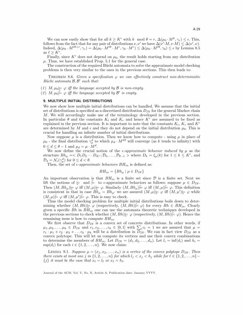
A:29

We can now easily show that for all k ≥ Kε with k mod θ = r, ∆(µ0 ·Mk, γr) ≤ ε. This,follows from the fact that for any pair of distributions ν, ν′ we have ∆(ν′·M,ν·M) ≤ ∆(ν′, ν).Indeed, ∆(µ0 ·M `θ+r, γr) = ∆(µ0 ·M `θ ·Mr, γ0 ·Mr) ≤ ∆(µ0 ·M `θ, γ0) ≤ ε by Lemma 8.5as ` ≥ Kε.

Finally, since Kε does not depend on µ0, the result holds starting from any distributionµ. Thus, we have established Prop. 5.1 for the general case.

The construction of the required Buchi automata to solve the approximate model checkingproblems is then very similar to the ones in the previous sections. This then leads to:

Theorem 8.6. Given a specification ϕ we can effectively construct non-deterministicBuchi automata B,B′ such that:

(1 ) M,µ0|=ε ϕ iff the language accepted by B is non-empty.(2 ) M,µ0|=

ε


9. MULTIPLE INITIAL DISTRIBUTIONS

We now show how multiple initial distributions can be handled. We assume that the initialset of distributions is specified as a discretized distribution DIN for the general Markov chainM . We will accordingly make use of the terminology developed in the previous section.In particular θ and the constants Kt and Kr and hence Kε are assumed to be fixed asexplained in the previous section. It is important to note that the constants Kt, Kr and Kε

are determined by M and ε and they do not depend on the initial distribution µ0. This iscrucial for handling an infinite number of initial distributions.

Now suppose µ is a distribution. Then we know how to compute - using µ in place ofµ0 - the final distribution γdµ to which µd ·Mkθ will converge (as k tends to infinity) with

0 ≤ d ≤ θ − 1 and µd = µ ·Md.We now define the crucial notion of the ε-approximate behavior induced by µ as the

structure Bhµ =< D1D2 · · ·DKε ;D0, . . . ,Dθ−1 > where Dk = ξµ(k) for 1 ≤ k ≤ Kε, andDd = Nε(γdµ) for 0 ≤ d < θ.

Then, the set of ε-approximate behaviors BHin is defined as:

BHin = {Bhµ | µ ∈ DIN }

An important observation is that BHin is a finite set since D is a finite set. Next welift the notions of |=ε and |=ε to ε-approximate behaviors as follows: suppose µ ∈ DIN .Then (M,Bhµ)|=

εϕ iff (M,µ)|=

εϕ. Similarly (M,Bhµ)|=ε ϕ iff (M,µ)|=ε ϕ. This definition

is consistent in that in case Bhµ = Bhµ′ we are assured (M,µ)|=εϕ iff (M,µ′)|=

εϕ while

(M,µ)|=ε ϕ iff (M,µ′)|=ε ϕ. This is easy to check.Thus the model checking problem for multiple initial distributions boils down to deter-

mining whether (M,Bh)|=εϕ (respectively, (M,Bh)|=ε ϕ) for every Bh ∈ BHin. Clearly

given a specific Bh in BHin one can use the automata theoretic techniques developed inthe previous sections to check whether (M,Bh)|=ε ϕ (respectively, (M,Bh)|=ε ϕ). Hence theremaining issue is how to compute BHin.

We first observe that DIN is a convex set of concrete distributions. In other words, ifµ1, µ2, . . . , µk ∈ DIN and c1, c2, . . . , ck ∈ [0, 1] with

∑l cl = 1 we are assured that µ =

c1 · µ1 + c2 · µ2 + . . . ck · µk will be a distribution in DIN . We can in fact view DIN as aconvex polytope. This will let us compute its vertices and use their convex combinationsto determine the members of BHin. Let DIN = (d1, d2, . . . , dn). Let li = inf(di) and hi =sup(di) for each i ∈ {1, 2, . . . , n}. We now claim:

Lemma 9.1. Suppose µ = (x1, x2, . . . , xn) is a vertex of the convex polytope DIN . Thenthere exists at most one j in {1, 2, . . . , n} for which lj < xj < hj while for ` ∈ {1, 2, . . . , n}−{j} it must be the case that x` = l` or x` = h`.


A:30

Proof. Suppose 1 ≤ j < k ≤ n, lj < xj < hj and lk < xk < hk. Let δ = min{xj −lj , hj − xj , xk − lk, hk − xk}. Let µ′ be given by µ′(i) = µ(i) if i ∈ {1, 2, . . . , n} − {j, k},µ′(j) = µ(j) − δ and µ′(k) = µ(k) + δ. Then it is easy to see that µ′ ∈ DIN and µ′ 6= µ.Next let µ′′ be given by µ′′(i) = µ(i) if i ∈ {1, 2, . . . , n} − {j, k}, µ′′(j) = µ(j) + δ andµ′′(k) = µ(k)−δ. Again it is easy to see that µ′′ ∈ DIN and µ′′ 6= µ. But then 1

2 ·µ′+ 1

2 ·µ′′ = µ

which contradicts the hypothesis that µ is a vertex.

Using the above lemma and the constraint x1 +x2 . . .+xn = 1 we can effectively computethe vertices of the polytope DIN . We let this set of vertices be V = {κ1, κ2, . . . , κJ} ⊆ DIN .We are assured that for each µ ∈ DIN there exist e1, e2, . . . , eJ ∈ [0, 1] such that

∑` e` = 1

and µ = e1 · κ1 + e2 · κ2 + . . .+ eJ · κJ .We next wish to show that the final distributions induced by a distribution µ ∈ DIN can

be represented as a convex combination of the final distributions induced by the vertices.To make this precise, for each µ ∈ DIN , let wµ be the weight vector induced by µ overthe components of M . Let γµ be the final distribution induced by µ as computed in theprevious section.

Proposition 9.2. Let ν =∑

1≤q≤J eqκq with eq ∈ [0, 1] and∑

1≤q≤J eu = 1. Then

γν =∑

1≤q≤J eqγκq .

Proof. This follows easily from the linearity of M , i.e, (aκ+ bκ′)M = aκM + bκ′M .

By linearity, we also have a similar property for γdµ = γµ ·Md, 0 ≤ d < θ. Hence, we onlyneed to explicitly compute γκ for every vertex κ ∈ V . Now, given a sequence D1 · · ·DKε ∈ Dand a θ-tuple of sets (D0,D1, . . . ,Dθ−1) with Di ⊆ D we can decide whether there existeq ∈ [0, 1] with 1 ≤ q ≤ J such that

—∑

1≤q≤J eq = 1,

— for all k < Kε,∑

1≤q≤J eqMk(κq) ∈ Dk, and

— for all 0 ≤ m ≤ θ − 1, Nε(∑

1≤q≤J eqγmκq ) = Dm.

We can decide this using the first order theory of reals. Consequently we can computethe finite set of ε-approximate behaviors of M generated by the distributions in DIN . Asnoted earlier, for each ε-approximate behavior in this set, we can decide if it meets thespecification ϕ and by taking the conjunction of all the outcomes we can decide whether(M,DIN )|=

εϕ and also whether (M,DIN )|=ε ϕ.

10. CONCLUSION

We have initiated here the study of the symbolic dynamics of finite state Markov chainsobtained by discretizing the probability value space [0, 1] into a finite set of intervals. Wehave shown that the symbolic dynamics of a Markov chain may not be ω-regular even if Mis irreducible and aperiodic.

We have designed a linear time temporal logic to reason about the symbolic dynamicsand have considered two variants of an approximate model checking problem in this setting.Our main result is that both the variants are decidable for the full class of Markov chains.

In the present study we have used a discretized distribution to specify the initial set ofdistributions. One can also use the convex hull of a finite set of rational valued concretedistributions to specify this set. Naturally one can then also allow a finite union of suchconvex polytopes to specify the set of initial distributions. With some additional work ourresults will easily extend to such sets of initial distributions. Further, as pointed out at theend of Section 6, we can also allow the atomic propositions to express polynomial constraintsover the components of the current distributions.

An interesting application to explore is the dynamics of biochemical networks modeledby the Chemical Master Equation [Wolf et al. 2010]. We feel that our symbolic dynamics


A:31

approach can bring considerable benefits in this setting. Further applications can openup by extending our results to the setting of Markov decision processes (MDPs). As anorthogonal extension, one can also explore the discretization of transition probabilities.This will involve working out the symbolic dynamics of interval Markov chains [Skulj 2009;Kozine 2002; Jonsson and Larsen 1991; Chatterjee et al. 2008; Benedikt et al. 2013] andperhaps even further generalizations such as constraint Markov chains [Caillaud et al. 2011].This would constitute an interesting and fruitful extension of the present work.

As mentioned in the introduction, our main goal has been to prove decidability in as simplea fashion as possible without paying much attention to complexity issues. We are howeverconfident that geometric representations and linear algebraic techniques can considerablylower the complexity of many of our constructions. In particular, a more careful computationof Kε for specific classes of Markov chains can be performed using results from the theory ofconvergence properties of Markov chains (e.g., from [Meyn and Tweedie 1993]). This couldlead to a significant improvement of our algorithm from a practical stand-point. We plan toaddress this issue in conjunction with an implementation of our model checking procedureand its applications in our future work.

Finally, in a number of settings one can generalize results from Markov chains to moregeneral linear operators [Seneta 1981]. It will be interesting to explore whether using suchtechniques our symbolic dynamics based verification techniques can be extended to moregeneral linear operators.

ACKNOWLEDGMENTS

We thank Joel Ouaknine and James Worrell for interesting and helpful discussions. Part of this work wasdone while Manindra Agrawal was visiting the IMS Workshop on Automata Theory at National University

of Singapore. Support from the workshop and J C Bose Fellowship is gratefully acknowledged. S. Akshay

would also like to acknowledge partial support from DST-INSPIRE faculty award [IFA12-MA-17] and ANRproject ImpRo (ANR-2010-BLAN-0317). Finally, Blaise Genest acknowledges partial support from ANR

projet STOCH-MC (ANR-13-BS02-0011-01) and EU project DISC and P.S. Thiagarajan acknowledges

partial support from the Singapore Ministry of Education grant MOE2011-T2-2-012.

REFERENCES

Agrawal, M., Akshay, S., Genest, B., and Thiagarajan, P. S. 2012. Approximate verification of thesymbolic dynamics of Markov chains. In LICS. IEEE Computer Society, 55–64.

Alur, R. and Dill, D. 1994. A theory of timed automata. TCS 126, 183–235.

Baier, C., Clarke, E., Hartonas-Garmhausen, V., Kwiatkowska, M., and Ryan, M. 1997. Symbolicmodel checking for probabilistic processes. In ICALP’97, LNCS. Vol. 1256. Springer, 430–440.

Baier, C., Haverkort, B., Hermanns, H., and Katoen, J.-P. 2005. Model checking meets performanceevaluation. ACM Performance Evaluation Review 32, 4, 10–15.

Baier, C., Hermanns, H., Katoen, J.-P., and Wolf, V. 2003. Comparative branching-time semantics forMarkov chains. In CONCUR’03. 482–497.

Baier, C. and Katoen, J.-P. 2008. Principles of Model Checking. MIT Press.

Beauquier, D., Rabinovich, A., and Slissenko, A. 2002. A logic of probability with decidable modelchecking. In CSL’02. 306–321.

Benedikt, M., Lenhardt, R., and Worrell, J. 2013. LTL model checking of interval Markov chains. InTACAS. 32–46.

Buchi, J. 1962. On a decision method in restricted second order arithmetic. In Int. Congress for Logic,Methodology and Philosophy of Science. Stanford University Press, 1–11.

Caillaud, B., Delahaye, B., Larsen, K. G., Legay, A., Pedersen, M. L., and Wasowski, A. 2011.Constraint Markov chains. Theor. Comput. Sci. 412, 34, 4373–4404.

Calbrix, H., Nivat, M., and Podelski, A. 1994. Ultimately periodic words of rational omega-languages.In Int. Conf. on Mathematical Foundations of Programming Semantics. Springer, 554–566.

Chadha, R., Korthikanti, V., Vishwanathan, M., Agha, G., and Kwon, Y. 2011. Model checking MDPswith a unique compact invariant set of distributions. In QEST’11.


A:32

Chatterjee, K., Sen, K., and Henzinger, T. A. 2008. Model-checking omega-regular properties of intervalMarkov chains. In FoSSaCS. 302–317.

Dedekind, R. 1996. Theory of Algebraic Integers. Cambridge Mathematical Library. Cambridge UniversityPress.

Delahaye, B., Larsen, K. G., Legay, A., Pedersen, M. L., and Wasowski, A. 2011. Decision problemsfor interval Markov chains. In LATA. 274–285.

Forejt, V., Kwiatkowska, M. Z., Norman, G., and Parker, D. 2011. Automated verification techniquesfor probabilistic systems. In SFM’11, LNCS. Vol. 6659. springer, 53–113.

Haddad, S. and Pekergin, N. 2009. Using stochastic comparison for efficient model checking of uncertainMarkov chains. In QEST. 177–186.

Hansson, H. and Jonsson, B. 1994. A logic for reasoning about time and reliability. Formal Asp. Com-put. 6, 5, 512–535.

Hardy, G. and Wright, E. 1960. An introduction to the Theory of Numbers. Clarendon Press, Oxford.

Henzinger, T. A. 1996. The theory of hybrid automata. In LICS. IEEE Computer Society, 278–292.

Huth, M. and Kwiatkowska, M. Z. 1997. Quantitative analysis and model checking. In LICS. IEEEComputer Society, 111–122.

Jonsson, B. and Larsen, K. G. 1991. Specification and refinement of probabilistic processes. In LICS.266–277.

Kemeny, J. G. and Snell, J. L. 1960. Finite Markov chains. Princeton university press.

Korthikanti, V. A., Viswanathan, M., Agha, G., and Kwon, Y. 2010. Reasoning about MDPs astransformers of probability distributions. In QEST. IEEE Computer Society, 199–208.

Kozine, I. O. 2002. Interval-valued Markov chains. Reliable Computing 8, 97– 113.

Kwiatkowska, M. Z., Norman, G., and Parker, D. 2011. Prism 4.0: Verification of probabilistic real-timesystems. In CAV. Lecture Notes in Computer Science Series, vol. 6806. Springer, 585–591.

Kwon, Y. and Agha, G. 2004. Linear inequality LTL (iLTL): A model checker for discrete time Markovchains. In ICFEM. Lecture Notes in Computer Science Series, vol. 3308. Springer, 194–208.

Kwon, Y. and Agha, G. 2011. Verifying the evolution of probability distributions governed by a DTMC.IEEE Trans. Software Eng. 37, 1, 126–141.

Lalley, S. 2010. Course notes: Basic Markov chain theory. website: http://galton.uchicago.edu/˜ lal-ley/Courses/312/MarkovChains.pdf.

Lang, S. 1994. Algebraic Number Theory (Graduate Texts in Mathematics). Springer.

Lind, D. and Marcus, B. 1995. An Introduction to Symbolic Dynamics and Coding. Cambridge UniversityPress, Cambridge.

Meyn, S. and Tweedie, R. 1993. Markov chains and stochastic stability. Springer-Verlag, London.

Mieghem, P. V. 2006. Performance Analysis of Communications Networks and Systems. Cambridge Uni-versity Press.

Morse, M. and Hedlund, G. A. 1938. Symbolic dynamics. American Journal of Mathematics 60, 815–866.

Norris, J. R. 1997. Markov chains. Cambridge series on statistical and probabilistic mathematics Series,vol. 2. Cambridge University Press, New York.

Ouaknine, J. and Worrell, J. 2012. Decision problems for linear recurrence sequences. In RP. 21–28.

Schneider, H. 2002. Wielandt’s proof of the exponent inequality for primitive nonnegative matrices. LinearAlgebra and its Applications 353, 5 – 10.

Seneta, E. 1981. Non-negative Matrices and Markov Chains. Springer series in Statistics. Springer.

Skulj, D. 2009. Discrete time Markov chains with interval probabilities. Int. J. Approx. Reasoning 50, 8,1314–1329.

Tarski, A. 1951. A Decision Method for Elementary Algebra and Geometry. Univ. of California Press.

Turakainen, P. 1968. On Stochastic Languagaes. Information and Control 12, 304–313.

Vardi, M. Y. 1999. Probabilistic linear-time model checking: An overview of the automata-theoretic ap-proach. In ARTS. Lecture Notes in Computer Science Series, vol. 1601. Springer, 265–276.

Weichselberger, K. 2000. The theory of interval-probability as a unifying concept for uncertainty. Int. J.Approx. Reasoning 24, 2-3, 149–170.

Wielandt, H. 1950. Unzerlegbare, nicht negative Matrizen, Math. Z. 52 (1950) 642-648 and MathematischeWerke/Mathematical Works, vol. 2, 100-106 de Gruyter, Berlin, 1996.

Wolf, V., Goel, R., and M. Mateescu, T. H. 2010. Solving the chemical master equation using slidingwindows. BMC Systems Biology 4:42.


Documents

Approximate Verification of the Symbolic Dynamics of