APPROXIMATION ALGORITHMS FOR NONUNIFORM BUY-AT

SIAM J. COMPUT. c© 2010 Society for Industrial and Applied MathematicsVol. 39, No. 5, pp. 1772–1798

APPROXIMATION ALGORITHMS FOR NONUNIFORMBUY-AT-BULK NETWORK DESIGN∗

C. CHEKURI† , M. T. HAJIAGHAYI‡ , G. KORTSARZ§ , AND M. R. SALAVATIPOUR¶

Abstract. Buy-at-bulk network design problems arise in settings where the costs for purchasingor installing equipment exhibit economies of scale. The objective is to build a network of cheapestcost to support a given multicommodity flow demand between node pairs. We present approximationalgorithms for buy-at-bulk network design problems with costs on both edges and nodes of an undi-rected graph. Our main result is the first poly-logarithmic approximation ratio for the non-uniformproblem that allows different cost functions on each edge and node; the ratio we achieve is O(log4 h),where h is the number of demand pairs. In addition we present an O(log h) approximation for thesingle sink problem. Poly-logarithmic ratios for some related problems are also obtained. Our algo-rithm for the multicommodity problem is obtained via a reduction to the single source problem usingthe notion of junction trees. We believe that this presents a simple yet useful general technique fornetwork design problems.

Key words. nonuniform buy-at-bulk, network design, approximation algorithm, concave cost,network flow, economies of scale

AMS subject classifications. 68Q25, 68W25, 90C27, 90C59

DOI. 10.1137/090750317

1. Introduction. Network design problems involve finding a minimum cost(sub) network that satisfies various properties, often involving connectivity and rout-ing between node pairs. Simple examples include spanning trees, Steiner trees, min-imum cost maximum flow, and k-connected subgraphs. These problems are of fun-damental importance in combinatorial optimization and also arise in a number ofapplications in computer science and operations research. Often, the cost in a typicalnetwork design problem is some function of the chosen edges or nodes.

Buy-at-bulk network design problems arise in settings where economies of scaleand the availability of capacity in discrete units result in concave or subadditive1 costfunctions on the edges or nodes. One of the main application areas is in the designof telecommunication networks. The typical scenario is that capacity (or bandwidth)on a link can be purchased in some discrete units u1 < u2 < · · · < ur with costsc1 < c2 < · · · < cr such that the cost per bandwidth decreases c1/u1 ≥ c2/u2 ≥ · · · ≥

∗Received by the editors February 20, 2008; accepted for publication (in revised form) September23, 2009; published electronically January 22, 2010. Most of the results of this paper appeared inpreliminary form in two extended abstracts [Proceedings of the IEEE Symposium on Foundations ofComputer Science, 2006] and [Proceedings of the ACM-SIAM Symposium on Discrete Algorithms,2007].

http://www.siam.org/journals/sicomp/39-5/75031.html†Department of Computer Science, University of Illinois, Urbana, IL 61801 ([email protected].

edu). This work was mostly done while the author was at Lucent Bell Labs. This author’s researchwas partly supported by NSF grant CCF-0728782.

‡AT&T Labs–Research, Florham Park, NJ 07932 ([email protected]). This work wasdone while the author was at the Department of Computer Science, Carnegie Mellon University,Pittsburgh, PA.

§Department of Computer Science, Rutgers University-Camden, Camden, NJ 08102 ([email protected]). This author’s reasearch was supported in part by NSF grant CCF-0829959.

¶Department of Computing Science, University of Alberta, Edmonton, AB T6G 2E8, Canada([email protected]). This author’s work was supported by NSERC grant G121210990 and afaculty start-up grant from the University of Alberta.

1A real-valued function f is subadditive if f(x) + f(y) ≥ f(x+ y) for all x, y ≥ 0.

1772

NONUNIFORM BUY-AT-BULK NETWORK DESIGN 1773

cr/ur. The capacity units are sometimes referred to as cables or pipes. The cablesinduce a monotone concave (or more generally a subadditive) function f : R+ → R

+,where f(b) is the minimum cost of cables of total capacity at least b. A basic problemthat needs to be solved in this setting is the following: given a set of bandwidthdemands, install sufficient capacity on the links of an underlying network topologyso as to be able to route the demands. Formally, we are given an undirected graphG = (V,E) on n nodes that represents the network topology and a set of h demandpairs T = {s1t1, s2t2, . . . , shth}. We refer to the end points of the pairs as terminals.Pair i has a nonnegative demand δ(i). Routing of the demands consists of findinga feasible multicommodity flow for the pairs in which δ(i) flow is sent from si to ti.The objective is to minimize the cost of the flow. The cost of the flow is given by∑

e∈E f(xe), where xe is the total flow on edge e. In this paper we consider a moregeneral problem where the function f can vary depending on the edge; that is, for eachedge e ∈ E there is a given monotone subadditive cost function fe : R+ → R

+. Thegoal is still to find a minimum cost feasible multicommodity flow for the demands; thecost of the flow in the more general setting is

∑e∈E fe(xe). We refer to this problem

as MC (multicommodity buy-at-bulk).We refer to the simpler case where the fe is the same for all edges as the uniform

problem and the general case as the nonuniform problem. An instance is called asingle-sink (or single-source) instance if all the pairs have a common sink (source) s;the pairs are of the form st1, st2, . . . , stk. We use SS to refer to this special case ofMC. A typical telecommunications problem with discrete capacity units gives rise to auniform problem. However, nonuniform cases arise often for several reasons, includingthe following: First, not all capacity units are available at all links, due to variousconstraints. Second, when designing networks incrementally, existing links can havedifferent unused capacity available, and this leads to nonuniformity.

Our discussion so far allowed costs on the edges of the network. A natural anduseful generalization is to allow costs (or weights) on both edges and nodes of thegraph. We are motivated to study this generalization by both theoretical as well aspractical considerations. For example, in telecommunications, expensive equipmentsuch as routers and switches are at the nodes of the underlying network, and itis natural to model some of these problems as node-weighted problems. Sometimes,costs on the nodes can be translated into costs on the edges in an approximate fashionto simplify the problems. However, this requires us to work with directed graphs, andproblems on directed graphs are typically more complex (harder to approximate forinstance) than the ones in undirected graphs, and hence it is desirable to work directlyon node-weighted problems in undirected graphs. For buy-at-bulk network design wecan easily reduce a problem in which both the nodes and edges have costs to theproblem in which only nodes have costs. In this paper we consider the buy-at-bulknetwork design problem with costs on the nodes. We formally define it now. The inputto the problem is the same as that for the edge-weighted case: an undirected graphG and a set T = {s1t1, s2t2, . . . , shth} of h node pairs with each pair siti specifying anonnegative demand δ(i). Each node v ∈ V has a monotone subadditive real-valuedfunction fv : R

+ → R+ associated with it. Again, a feasible solution consists of

finding a feasible multicommodity flow for the pairs in which δ(i) flow is sent from sito ti. As we will see later, by losing at most a ratio of 2 + ε (for any constant ε > 0)in the approximation, we may assume that the flow in the solution is unsplittable.Namely, the solution may be considered as a collection P1, P2, . . . , Ph of paths suchthat Pi connects si and ti and the demand δ(i) is routed along path Pi. The cost

1774 CHEKURI, HAJIAGHAYI, KORTSARZ, AND SALAVATIPOUR

of the flow is∑

v∈V fv(xv), where xv is the total flow that is routed through a nodev, namely, xv =

∑i|v∈Pi

δ(i). We assume that a flow that originates at a node v is

also routed through v. The objective is to find a feasible solution (or routing) for thepairs that minimizes the total cost. We refer to this problem as NMC (node-weightedmulticommodity buy-at-bulk). The single-sink version is referred to as NSS.

We focus for the most part on NMC and NSS, since they generalize MC and SS,respectively. Although there are many papers that have studied the edge-weightedversions of the problems, we are not aware of any result that studied the more generalversions NMC and NSS. Buy-at-bulk network design problems capture as special casesome classical NP-hard connectivity problems, such as minimum cost Steiner treeand Steiner forest problems; unlike these connectivity problems that admit constant-factor approximation ratios [32, 4], it was shown by Andrews [1] that unless NP ⊆ZTIME

(npolylog(n)

), MC does not admit a log

12−ε n-approximation for any fixed

ε > 0.Our main result is the following.Theorem 1.1. There is a polynomial time O(log4 h)-ratio approximation algo-

rithm for NMC, where h is the number of pairs.The algorithm of this theorem is based on rounding a solution to a linear program-

ming (LP) relaxation. We also present a greedy combinatorial algorithm for the edge-

weighted version, i.e., MC, that yields a ratio of O(log3 h logD); here D =∑h

i=1 δ(i)is the sum of the demands of the input pairs with mini δ(i) normalized to be 1. Thegreedy algorithm has the advantage of being simple and combinatorial and revealsuseful insights into the problem structure; it is also asymptotically more efficient thanthe LP-based algorithm.

Our algorithms for the multicommodity problems are built upon their single-sinkcounterparts. For the edge-cost SS problem an O(log h)-approximation was given by[30]. We give an algorithm for the node-cost version.

Theorem 1.2. There is a deterministic O(log h)-approximation algorithm forNSS, where h is the number of terminals. Furthermore, the integrality gap of a naturalLP relaxation for the problem is O(log h).

An easy reduction from the set cover problem shows that unless P = NP , thenode-weighted Steiner tree problem [25], a special case of NSS, cannot be approxi-mated to a ratio better than c log h for some universal constant c [28, 31]. Thus theratio guaranteed by Theorem 1.2 cannot be improved by more than a constant factorunless P = NP .

We also consider a variant of NMC and NSS that requires only a subset of pairsto be connected. Let T = {s1t1, s2t2, . . . , shth}. For a subset T ′ ⊆ T , we let opt(T ′)denote the cost of an optimum solution that connects the pairs in T ′. In the densityproblem, we seek to find a subset of pairs T ′ such that opt(T ′)/|T ′| is minimized.We use den-NMC and den-NSS to refer to the density versions of NMC and NSS;similarly den-MC and den-SS for the density versions of MC and SS. We prove thefollowing theorem, which in turn is used in the proof of Theorem 1.1.

Theorem 1.3. There is a polynomial time O(log2 h)-approximation for den-NSS.

1.1. Related work. Network design problems are of fundamental importancein combinatorial optimization, and there is a vast literature on problems and results.We refer the reader to [33] for classical results on polynomial time algorithms and to[19, 20, 36, 23, 12] for results and pointers on approximation algorithms. Here webriefly discuss the known results and techniques for some specific problems that areclosely related to the problems we consider.


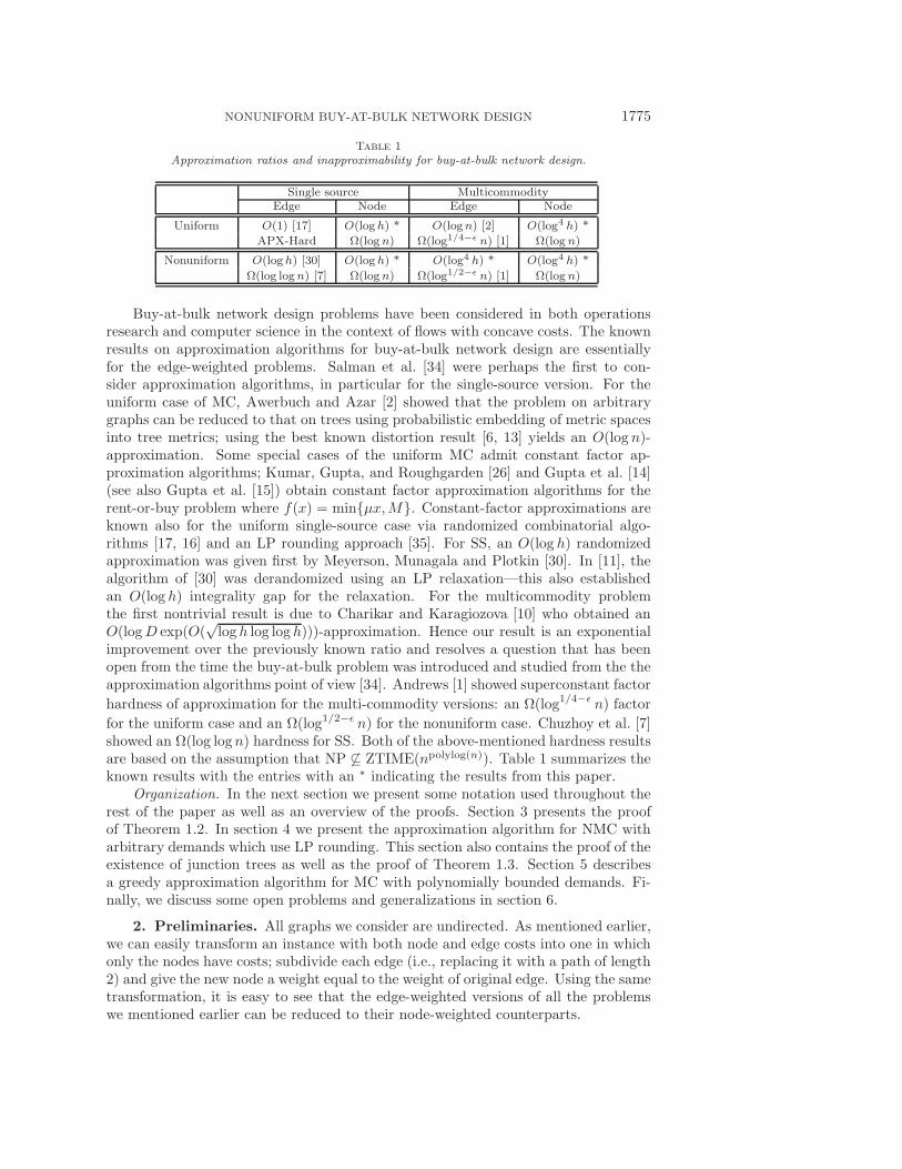
Table 1

Approximation ratios and inapproximability for buy-at-bulk network design.

Single source MulticommodityEdge Node Edge Node

Uniform O(1) [17] O(log h) * O(logn) [2] O(log4 h) *

APX-Hard Ω(logn) Ω(log1/4−ε n) [1] Ω(log n)

Nonuniform O(log h) [30] O(log h) * O(log4 h) * O(log4 h) *

Ω(log logn) [7] Ω(logn) Ω(log1/2−ε n) [1] Ω(log n)

Buy-at-bulk network design problems have been considered in both operationsresearch and computer science in the context of flows with concave costs. The knownresults on approximation algorithms for buy-at-bulk network design are essentiallyfor the edge-weighted problems. Salman et al. [34] were perhaps the first to con-sider approximation algorithms, in particular for the single-source version. For theuniform case of MC, Awerbuch and Azar [2] showed that the problem on arbitrarygraphs can be reduced to that on trees using probabilistic embedding of metric spacesinto tree metrics; using the best known distortion result [6, 13] yields an O(log n)-approximation. Some special cases of the uniform MC admit constant factor ap-proximation algorithms; Kumar, Gupta, and Roughgarden [26] and Gupta et al. [14](see also Gupta et al. [15]) obtain constant factor approximation algorithms for therent-or-buy problem where f(x) = min{μx,M}. Constant-factor approximations areknown also for the uniform single-source case via randomized combinatorial algo-rithms [17, 16] and an LP rounding approach [35]. For SS, an O(log h) randomizedapproximation was given first by Meyerson, Munagala and Plotkin [30]. In [11], thealgorithm of [30] was derandomized using an LP relaxation—this also establishedan O(log h) integrality gap for the relaxation. For the multicommodity problemthe first nontrivial result is due to Charikar and Karagiozova [10] who obtained anO(logD exp(O(

√log h log log h)))-approximation. Hence our result is an exponential

improvement over the previously known ratio and resolves a question that has beenopen from the time the buy-at-bulk problem was introduced and studied from the theapproximation algorithms point of view [34]. Andrews [1] showed superconstant factor

hardness of approximation for the multi-commodity versions: an Ω(log1/4−ε n) factor

for the uniform case and an Ω(log1/2−ε n) for the nonuniform case. Chuzhoy et al. [7]showed an Ω(log logn) hardness for SS. Both of the above-mentioned hardness resultsare based on the assumption that NP �⊆ ZTIME(npolylog(n)). Table 1 summarizes theknown results with the entries with an ∗ indicating the results from this paper.

Organization. In the next section we present some notation used throughout therest of the paper as well as an overview of the proofs. Section 3 presents the proofof Theorem 1.2. In section 4 we present the approximation algorithm for NMC witharbitrary demands which use LP rounding. This section also contains the proof of theexistence of junction trees as well as the proof of Theorem 1.3. Section 5 describesa greedy approximation algorithm for MC with polynomially bounded demands. Fi-nally, we discuss some open problems and generalizations in section 6.

2. Preliminaries. All graphs we consider are undirected. As mentioned earlier,we can easily transform an instance with both node and edge costs into one in whichonly the nodes have costs; subdivide each edge (i.e., replacing it with a path of length2) and give the new node a weight equal to the weight of original edge. Using the sametransformation, it is easy to see that the edge-weighted versions of all the problemswe mentioned earlier can be reduced to their node-weighted counterparts.


It is algorithmically convenient to reduce the buy-at-bulk problem to a two-costnetwork design problem [3, 30]. This involves approximating the monotone sub-additive cost function fv for each v by a collection of linear cost functions as fol-lows. We assume without loss of generality that the demand values δ(i) for eachpair siti are nonnegative integers. Let D =

∑i δ(i) be the total demand. Let

ε > 0 be any fixed constant. For 1 ≤ i ≤ logD we define f iv : R

+ → R+

as f iv(x) = fv((1 + ε)i)(1 + x/(1 + ε)i). We replace v by a collection of nodes

Sv = {vi : 1 ≤ i ≤ logD}, and the function associated with vi is f iv. If uv

was an edge in the original graph G, we add edges uivj for all pairs i, j. Note thatin the new instance each function is of the form a + bx. It can be verified that thistransformation loses at most a factor of 2 + ε in the approximation ratio. The linearfunctions allow us to reformulate the objective function of the buy-at-bulk networkdesign problem. In this setting, an instance of NMC consists of a graph G and de-mand pairs T = {s1t1, s2t2, . . . , shth}. Each si, ti ∈ V has a demand δ(i) ≥ 0. Weare given two separate functions c : V → R

+ and � : V → R+; we call c(v) and �(v)

the fixed-cost and length of v, respectively. We think of cv as the fixed-cost of buyingv to use it and �v as the incremental or flow-cost of v. The goal is to find a minimumtotal cost to refer to the solution where a feasible solution consists of a subset of nodesV ′ ⊆ V that include all the terminals. The subset V ′ implicitly specifies the inducedsubgraph G′ = G[V ′]. The total cost of the solution specified by V ′ is given as

(1) c(V ′) +h∑

i=1

δ(i) · �G′(si, ti),

where c(V ′) =∑

v∈V ′ cv and �G′(u, v) is the shortest �-node-weighted path distancebetween u and v in G′ (the length of the end points of a path are counted as well).2 Asjust shown, the two-cost formulation shows that the optimum cost for the unsplittableflow version of the problem is at most a constant factor more than the optimum costof a solution that allows the flow for each pair to be split among multiple paths. In therest of the paper, we restrict our attention to the two-cost network design formulationof NMC and NSS (and similarly for MC).

Let T denote the set of source-sink pairs in the given instance and h = |T |. Thevariable h′ is used to denote the number of uncovered pairs remaining at some stageof the algorithm. If all demands δ(i) are equal, then, by scaling down the demandsand the costs, we can assume all demands are equal to 1. For this reason we refer to itas a unit-demand instance. We assume without loss of generality that each terminalis a node of degree 1 and that exactly 1 pair contains each terminal. This can beachieved by hanging dummy terminals.

In the rest of the paper, when we refer to an optimum solution to a given instance,we assume some fixed optimum solution. We use opt to denote its (total) cost.The optimum solution’s fixed-cost (i.e., first term in (1)) and length (second termin (1)) are denoted by optc and opt�, respectively. Note that by definition opt =optc + opt�. If the graph G[V ′] contains an si to ti path, we say that V ′ routes orcovers the pair si, ti. The set of pairs routed in G[V ′] is denoted by T (V ′). AssumeT ′ = T (V ′) ⊂ T does not contain all the source-sink pairs and that G[V ′] routes allthe pairs of T ′ but no other pair. The fixed-cost and length (incremental cost) of V ′

are c(V ′) =∑

v∈V ′ cv and R(V ′) =∑

i:siti∈T ′ δ(i) · �G[V ′](si, ti), respectively. The

2We use the term fixed-cost in a consistent way to distinguish it from the total cost, whichincludes both the fixed-costs and the incremental costs.


total cost of the partial solution V ′ is ψ(V ′) = c(V ′) + R(V ′). The total density ofpartial solution V ′ is ψ(V ′)/|T ′|. We also define the fixed-cost density and length-density of solution V ′ as c(V ′)/|T ′| and R(V ′)/|T ′|, respectively.

We may drop some of the parameters in our notation if they can be deduced fromthe context. Unless specified differently all log’s are in base 2. Our algorithms forNMC and MC are greedy iterative algorithms. In each iteration the algorithm findsa partial solution (a solution that routes some of the remaining uncovered demands)at low density, where the density is the ratio of the cost of the partial solution to thenumber of new demands it connects. We will use the following basic lemma in theanalysis of these algorithms (see, e.g., [24]).

Lemma 2.1. Suppose that an algorithm works in iterations, and in iteration i itfinds a partial solution Vi ⊆ V that routes a new subset Ti of the demands. Let optbe the (total) cost of an optimum solution and ui be the number of unrouted demandsat the time Vi is found. If for every i the (total) cost of the partial solution G[Vi]over the number of pairs it routes is at most f(h) · optui

, then the cost of the solutionreturned by the algorithm is at most f(h) · (lnh+ 1) · opt.

2.1. Overview of algorithmic ideas. We briefly outline the high-level ideasbehind our algorithm for NMC. The algorithm follows a greedy scheme in an iterativefashion. In each iteration it finds a partial solution that connects a subset of theuncovered pairs. The connected pairs are then removed. Recall that the density ofa partial solution is the ratio of the total cost of the partial solution to the numberof pairs in the solution. For some fixed constant a, the algorithm guarantees thatthe density of the partial solution it computes is at most O(loga h) ·opt′/|T ′|, whereT ′ is the set of remaining terminals at the beginning of the iteration and opt

′ isthe cost of an optimum solution for T ′. Using Lemma 2.1, this scheme yields anO(loga+1 h)-approximation.

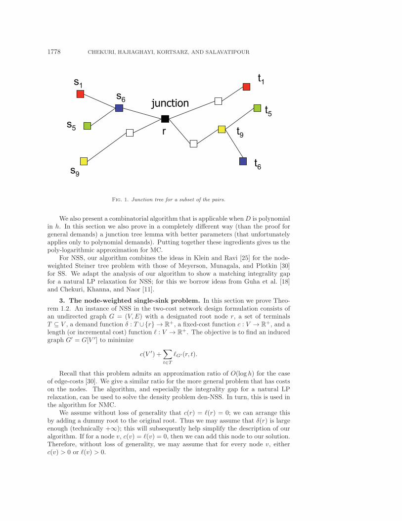
The key insight is to show the existence of a low-density partial solution that hasa restricted structure. This structure allows us to find a near-optimal partial solutionin polynomial time. The restricted structure of interest is what we call a junction tree(see Figure 1). Given a subset A of the pairs, a junction tree for A rooted at r is atree T containing the end points of all pairs in A such that for each pair in A, theunique path in T for the pair contains r. The cost of a junction tree T is

∑

v∈V (T )

cv +∑

siti∈A

δ(i) · (�T (r, si) + �T (r, ti)).

In other words, the pairs in A connect via the junction r. We prove that givenan instance of NMC, there is always a low-density partial solution that is a junction-tree. The problem of finding a low-density junction tree is closely related to thedensity variation of NSS, i.e., den-NSS. We use Theorem 1.2 and obtain an O(log2 h)-approximation for den-NSS and by a slight modification a similar ratio for finding aminimum-density junction tree. Putting together these ingredients give us the poly-logarithmic approximation for NMC. We observe that the above scheme effectivelyreduces the multicommodity problem to the single-sink problem, and this generalparadigm is of broader applicability.

The first method uses an LP relaxation to solve the problem approximately. ThisLP is similar to the LP relaxation for SS proposed in [11]. Using the O(log h) upperbound on its integrality gap, we obtain an O(log2 h)-approximation for den-SS andby a slight modification a similar ratio for finding the best-density junction tree.


junction

t1s

1

s5

t5

s6

t6

s9

t9

r

Fig. 1. Junction tree for a subset of the pairs.

We also present a combinatorial algorithm that is applicable whenD is polynomialin h. In this section we also prove in a completely different way (than the proof forgeneral demands) a junction tree lemma with better parameters (that unfortunatelyapplies only to polynomial demands). Putting together these ingredients gives us thepoly-logarithmic approximation for MC.

For NSS, our algorithm combines the ideas in Klein and Ravi [25] for the node-weighted Steiner tree problem with those of Meyerson, Munagala, and Plotkin [30]for SS. We adapt the analysis of our algorithm to show a matching integrality gapfor a natural LP relaxation for NSS; for this we borrow ideas from Guha et al. [18]and Chekuri, Khanna, and Naor [11].

3. The node-weighted single-sink problem. In this section we prove Theo-rem 1.2. An instance of NSS in the two-cost network design formulation consists ofan undirected graph G = (V,E) with a designated root node r, a set of terminalsT ⊆ V , a demand function δ : T ∪{r} → R

+, a fixed-cost function c : V → R+, and a

length (or incremental cost) function � : V → R+. The objective is to find an induced

graph G′ = G[V ′] to minimize

c(V ′) +∑

t∈T

�G′(r, t).

Recall that this problem admits an approximation ratio of O(log h) for the caseof edge-costs [30]. We give a similar ratio for the more general problem that has costson the nodes. The algorithm, and especially the integrality gap for a natural LPrelaxation, can be used to solve the density problem den-NSS. In turn, this is used inthe algorithm for NMC.

We assume without loss of generality that c(r) = �(r) = 0; we can arrange thisby adding a dummy root to the original root. Thus we may assume that δ(r) is largeenough (technically +∞); this will subsequently help simplify the description of ouralgorithm. If for a node v, c(v) = �(v) = 0, then we can add this node to our solution.Therefore, without loss of generality, we may assume that for every node v, eitherc(v) > 0 or �(v) > 0.


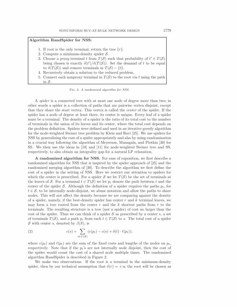
Algorithm RandSpider for NSS:

1. If root is the only terminal, return the tree {r}.2. Compute a minimum-density spider S.3. Choose a proxy terminal t from T (S) such that probability of t′ ∈ T (S)

being chosen is exactly δ(t′)/δ(T (S)). Set the demand of t to be equalto δ(T (S)) and remove terminals in T (S)− {t}.

4. Recursively obtain a solution to the reduced problem.5. Connect each nonproxy terminal in T (S) to the root via t using the path

in S.

Fig. 2. A randomized algorithm for NSS.

A spider is a connected tree with at most one node of degree more than two; inother words a spider is a collection of paths that are pairwise vertex disjoint, exceptthat they share the start vertex. This vertex is called the center of the spider. If thespider has a node of degree at least three, its center is unique. Every leaf of a spidermust be a terminal. The density of a spider is the ratio of its total cost to the numberof terminals in the union of its leaves and its center, where the total cost depends onthe problem definition. Spiders were defined and used in an iterative greedy algorithmfor the node-weighted Steiner tree problem by Klein and Ravi [25]. We use spiders forNSS by generalizing the cost of a spider appropriately and also by using randomizationin a crucial way following the algorithm of Meyerson, Munagala, and Plotkin [30] forSS. We then use the ideas in [18] and [11] for node-weighted Steiner tree and SS,respectively, to also obtain an integrality gap for a natural LP relaxation.

A randomized algorithm for NSS. For ease of exposition, we first describe arandomized algorithm for NSS that is inspired by the spider approach of [25] and therandomized merging algorithm of [30]. To describe the algorithm we first define thecost of a spider in the setting of NSS. Here we restrict our attention to spiders forwhich the center is prescribed. For a spider S we let T (S) be the set of terminals atthe leaves of S. For a terminal t ∈ T (S) we let pt denote the path between t and thecenter of the spider S. Although the definition of a spider requires the paths pt, fort ∈ S, to be internally node-disjoint, we abuse notation and allow the paths to sharenodes. This will not affect the density because we are comparing against the densityof a spider, namely, if the best-density spider has center r and k terminal leaves, wemay form a tree rooted from the center r and the k shortest paths from r to theterminals. The resulting structure is a tree (not a spider) of cost no larger than thecost of the spider. Thus we can think of a spider S as prescribed by a center s, a setof terminals T (S), and a path pt from each t ∈ T (S) to s. The total cost of a spiderS with center s, denoted by β(S), is

(2) c(s) +∑

t∈T (S)

(c(pt)− c(s) + δ(t) · �(pt)),

where c(pt) and �(pt) are the sum of the fixed costs and lengths of the nodes on pt,respectively. Note that if the pt’s are not internally node disjoint, then the cost ofthe spider would count the cost of a shared node multiple times. The randomizedalgorithm RandSpider is described in Figure 2.

We make two observations. If the root is a terminal in the minimum-densityspider, then by our technical assumption that δ(r) = +∞ the root will be chosen as


the proxy. In the last step, it is not necessary for a nonproxy terminal to connectto the proxy terminal using the path in spider S—there could be a cheaper directpath; however, the analysis carries through using the path in S. We can prove, usingideas similar to those in [30], that RandSpider yields a solution of expected costO(log h · opt), where opt is the cost of an optimum integral solution. We provea stronger theorem, which also yields a bound on the integrality gap of a naturalLP relaxation. First we show that a minimum density spider can be computed inpolynomial time.

For a terminal t and a node v we let dt(v) denote minp∈Ptv (c(p) + δ(t) · �(p)),where Ptv is the set of all paths between t and v. In other words dt(v) is the shortestpath distance between t and v with the weight of a node u set to c(u) + δ(t) · �(u).

Lemma 3.1. There is a polynomial time algorithm, that given an instance ofNSS, finds a minimum-density spider.

Proof. Let s be the center of a minimum-density spider. For each node v ∈ V werun an algorithm to be described below that computes a minimum-density spider withcenter v, and thus we can assume that we know s. For simplicity, we assume that s isnot a terminal—this can always be ensured by hanging dummy terminals. Withoutloss of generality assume that terminals are ordered such that dt1(s) ≤ dt2(s) ≤ · · · ≤dth(s). Let Pi be a path from ti to s that corresponds to distance dti(s). For 2 ≤ j ≤ h,let αj =

1j ·(c(s)+

∑1≤i≤j(dti(s)−c(s))) denote the density of a subgraph obtained by

connecting the first j terminals (in the ordering) to s. Let j∗ = argminjαj . We returnthe subgraph S obtained by the union of the paths P1, P2, . . . , Pj∗ . We show that thedensity of S is no more than the density of a minimum-density “real” spider (by realspider we mean a tree with internally disjoint nodes). Say that the best-density spiderhas j leaves. Note that j is one of the “guesses” of the number of terminals used bythe algorithm. The density of S is no larger than the density of the spider, as we takethe j shortest paths from s to the terminals.

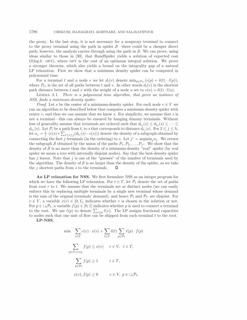
An LP relaxation for NSS. We first formulate NSS as an integer program forwhich we have the following LP relaxation. For t ∈ T , let Pt denote the set of pathsfrom root r to t. We assume that the terminals are at distinct nodes (we can easilyenforce this by replacing multiple terminals by a single new terminal whose demandis the sum of the original terminals’ demand), and hence Pt and Pt′ are disjoint. Forv ∈ V , a variable x(v) ∈ [0, 1], indicates whether v is chosen in the solution or not.For p ∈ ∪tPt, a variable f(p) ∈ [0, 1] indicates whether p is used to connect a terminalto the root. We use �(p) to denote

∑v∈p �(v). The LP assigns fractional capacities

to nodes such that one unit of flow can be shipped from each terminal t to the root.LP-NSS.

min∑

v∈V

c(v) · x(v) +∑

t∈T

δ(t)∑

p∈Pt

�(p) · f(p)

∑

p∈Pt|v∈p

f(p) ≤ x(v) v ∈ V, t ∈ T,

∑

p∈Pt

f(p) ≥ 1 t ∈ T ,

x(v), f(p) ≥ 0 v ∈ V, p ∈ ∪tPt.


Let optLP be the cost of an optimum solution to LP-NSS. We prove that Rand-Spider yields an integral solution of expected cost O(log h ·optLP ). The proof of thefollowing lemma uses ideas from [18] and is deferred to Appendix A.

Lemma 3.2. For any instance of NSS there is a spider of density at mostoptLP /h.

We assume the lemma and prove Theorem 1.2. We will show how to derandomizeRandSpider via the LP relaxation using ideas similar to [11]. Let I be the giveninstance, and let S be a minimum-density spider for I computed by RandSpider instep 2. Let I ′ be the reduced instance obtained after the proxy terminal from S ischosen in step 3 of the algorithm. Let optLP (I) and optLP (I

′) denote the optimumvalues of the linear program LP-NSS on instances I and I ′, respectively. Note thatoptLP (I

′) is a random variable.Lemma 3.3. E[optLP (I

′)] ≤ optLP (I).Proof. Let x∗, f∗ be an optimal feasible solution to the instance I. In the instance

I ′ we have essentially changed only the value of the demands; the proxy terminal getsa demand equal to δ(T (S)), while the removed terminals get demand 0. Thus thesolution x∗, f∗ is also a feasible solution to I ′. We show that the expected costof this solution for I ′ is the same as optLP (I). For terminal t ∈ Ti let α(t) =∑

p∈Pt�(p) · f∗(p). We have optLP (I) =

∑v∈V c(v) · x∗(v) +

∑t∈T δ(t) · α(t). For

every terminal t �∈ T (S), its contribution to the total cost remains unchanged in thesolution for I ′. On the other hand, the expected contribution of a terminal t ∈ T (S)in I ′ is exactly δ(t) · α(t) for the following reason; the probability that t is chosenas a proxy terminal is δ(t)/δ(T (S)), and if it is chosen, then the contribution isδ(T (S)) ·α(t). Thus it can be seen that the expected cost of the solution x∗, f∗ for I ′

is at most optLP (I).For a spider S let β(S) denote its cost as in (2).Lemma 3.4. In step 5 of RandSpider, the expected cost of routing nonproxy

terminals to the chosen proxy terminal is at most 2β(S).Proof. We can bound the expected cost as follows. The cost consists of two parts.

The first part accounts for the cost of each terminal t ∈ T (S) sending its demand to thecenter s of S. This cost is deterministically at most β(S), by definition. The secondpart accounts for the center sending the total demand δ(T (S)) to the chosen proxyterminal. The expected cost of this second part is seen to be

∑t∈T (S) at ·δ(T (S))·�(pt),

where at is the probability that t is chosen as the proxy terminal and pt is the pathfrom t to the center s in S. Since at = δ(t)/δ(T (S)), it follows that the expected costis

∑t∈T (S) δ(t)�(pt), which is at most β(S). Therefore the total expected cost is at

most 2β(S).Proof of Theorem 1.2. We first prove via induction on h that RandSpider yields

a solution of expected cost at most 3Hh · optLP , where Hh = 1 + 1/2 + · · · + 1/h isthe hth Harmonic number. This immediately proves that the integrality gap of LP-NSS is O(log h). We then sketch a way to derandomize RandSpider using pessimisticestimators.

Let I be the given instance of NSS. If h = 1, then it can be easily checked thatthe algorithm returns an optimum solution. This is because the case h = 1 is theproblem of finding a minimum node-cost path from the single terminal t to the rootr where the cost of a node v is defined to be c(v) + δ(t) · �(v); the algorithm for theminimum-density spider computes such a path correctly.

Consider the steps of RandSpider on I. Let S be the spider computed in step 2,and let k be the number of terminals in S. By Lemma 3.2, we have that β(S)/k ≤


optLP (I)/h. Let I ′ be the random problem that RandSpider generates in step 3.By induction, the expected cost of the solution produced by RandSpider to I ′ is atmost 3Hh′ · optLP (I

′), where h′ = h− k + 1 is the number of terminals in I ′. UsingLemma 3.3, this expected cost is at most 3Hh′ · optLP (I). The total cost of thesolution for I is the sum of two costs: (i) the cost of the solution to I ′ and (ii) the costof the routing of nonproxy terminals in S to the chosen proxy terminal. The expectedcost of (ii) is, by Lemma 3.4, bounded by 2β(S). Using Lemma 3.2 and the fact that Sis a minimum-density spider with k terminals, we have that 2β(S) ≤ 2koptLP (I)/h.Putting together these observations and using linearity of expectation, the expectedcost of the solution to I is at most

3Hh′ · optLP (I) + 2β(S) ≤ (3Hh′ + 2k/h)optLP (I)

≤ 3Hh · optLP (I).

The algorithm RandSpider can be derandomized using a solution to LP-NSS asdescribed below. The argument is essentially the same as the one in [11]. Let x∗, f∗

be a feasible solution to LP-NSS on I. In step 3 of the algorithm, instead of choosingthe proxy terminal in S at random, we can pick the terminal deterministically asfollows. For t ∈ T (S) let I ′t be the instance obtained if t is chosen as a proxy terminal,let βt be the cost of routing the terminals in T (S)−{t} to t using S, and let αt be thecost of the solution x∗, f∗ on I ′t. Note that αt and βt can be computed in polynomialtime from x∗, f∗ and S. Let t′ = argmint(3Hh′αt + 2βt). The above probabilisticanalysis shows that 3Hh′ · αt′ + 2βt′ ≤ 3Hh · optLP (I). We deterministically chooset′ to be the proxy terminal for S, solve the problem I ′t′ recursively, and connectthe terminals in T (S) − {t′} to the root via t′ using S. Inductively the cost ofthe solution on I ′t′ is at most 3Hh′ · αt′ . Therefore the total cost of the solution is3Hh′ · αt′ + 2βt′ ≤ 3Hh · optLP (I) as desired.

4. The node-weighted multicommodity problem. In this section we proveTheorems 1.1 and 1.3. The general structure of the algorithm of Theorem 1.1 fol-lows the outline described in section 2.1. We iteratively find a partial solution ofdensity that is comparable to that of an optimum solution on the remaining termi-nals. We prove that the density of the partial solution computed in each iteration isa poly-logarithmic (specifically O(log3 h)) factor away from the density of the opti-mum solution. By Lemma 2.1, an O(log4 h) ratio follows for the MC instance. Therest of this section is devoted to showing how to find a partial solution with densityO(log3 h) · opt/h.

As said earlier, a key ingredient in our proof is to show the existence of a gooddensity partial solution that is a junction tree. We first prove that given an instance ofNMC, there is always a junction tree of density O(log h) times the optimum density.Thus, to find a good density partial solution, it is sufficient to find a good densityjunction tree. If the root and the participating terminals in a junction tree are known,then a junction tree is essentially an instance of the single-sink problem NSS. There-fore, the problem of finding a low-density junction tree is closely related to the densityvariation of NSS, called den-NSS, in which we want to find a solution with minimumdensity, i.e., the ratio of total cost to the number of terminals spanned (versus thetotal value as in SS). We use Theorem 1.2 and obtain an O(log2 h)-approximation forden-NSS and by a slight modification a similar ratio for finding a minimum-densityjunction tree. Note that a difficulty we have to overcome (going from den-NSS to


computing a good density junction tree) is that we do not know the root and theparticipating pairs in the junction tree.

Note that in total we lose an O(log3 h) factor; an O(log2 h) loss is because thisis the approximation ratio for computing the density of a junction tree and a furtherO(log h) loss because the best-density junction tree may have density O(log h) worsethan the density of an optimum solution.

4.1. Junction tree lemma for general demands. We prove the followinglemma on the existence of a junction tree with low density.

Lemma 4.1. Given an instance of MC on h pairs, there exists a junction tree ofdensity O(log h) · opth .

The rest of this subsection is devoted to the proof of the above lemma. In [8]proofs are given for two lemmas with slightly weaker bounds, and a proof idea thatcombined aspects of both those lemmas was suggested by Harald Racke. We need thefollowing technical lemma first.

Lemma 4.2. Given an instance of NMC on G = (V,E) there is an optimumsolution G∗ = G[V ∗] such that the number of nodes in G∗ of degree more than 2 is atmost min(n, h2).

Proof. We have a trivial upper bound of n on the number of degree 2 nodes;thus we focus on proving the bound of h2. We assume without loss of generality thatthe terminals are all distinct; we can use dummy terminals as necessary. Consideran optimum solution G[V ∗]. Each pair siti uses a shortest �-node-weighted path Pi

in G[V ∗] to route its demand. We can assume that Pi is the unique shortest pathbetween si and ti; this can be arranged by considering a lexicographical ordering ofthe nodes and edges of G. Therefore, for any two distinct pairs siti and sjtj , Pi ∩ Pj

is connected.3 Thus the two paths may meet at some node, share a subpath for awhile, and then be separated and never meet again. Now consider inserting the pathsP1, P2, . . . , Ph in order. From the above observation, when Pi is inserted, for everyj < i, it can add at most two vertices of degree more than 2. Thus Pi can create atmost 2(i− 1) nodes of degree more than 2. Therefore, the total number of nodes with

degree strictly greater than 2 is bounded by∑h

i=1 2(i− 1) ≤ h2.Given an edge-weighted graphG = (V,E), let T = (VT , ET ) be a tree representing

a laminar family on V . We let dG(a, b) denote the distance in G between nodes a andb where the distance is defined with respect to the given edge-weights. For an internalnode u ∈ VT , let Tu be the subtree of T rooted at u. We denote by Gu the subgraphof G induced by the leaves in Tu. For a pair of nodes a, b ∈ V (G), let GT

a,b denotethe graph Gu, where u is the least common ancestor of a and b in T . We denote byΔT (a, b) the diameter of the graph GT

a,b. Note that, trivially, ΔT (a, b) ≥ dG(a, b),where dG(a, b) is the distance between a, b in G. Given G and a laminar family T , wesay that a pair of nodes a, b ∈ V (G) is α-good in T if and only if ΔT (a, b) ≤ α·dG(a, b).Before we can prove the junction tree lemma, we need to prove the following lemma.

Lemma 4.3. Given G and a set of node pairs A, there exists a laminar family Tand a constant c such that the number of pairs in A that are (2c logn)-good in T isat least |A|/4.

Now we prove the above lemma. Given an instance of NMC on a graph G =(V,E), let V ∗ ⊆ V induce an optimum solution for the given instance. UsingLemma 4.2, we can assume that G[V ∗] has O(min(n, h2)) nodes by suppressing non-terminals that have degree at most 2 in G∗. Recall that the cost of an optimum

3We thank Anupam Gupta for making this observation in answering a question about spanners.


solution, opt, is c(V ∗) +∑

i δi�G∗(si, ti), where �G∗(si, ti) is the �-node-weighteddistance between si and ti in G

∗.The crucial ingredient in the proof is the existence of a hierarchical decomposition

of an undirected edge-weighted graph that has certain useful properties to be describedbelow. Our focus is on node-weights, and we have two weight functions c and �. Inthe following we use � to define the edge-weights of G∗ by setting for each edgeuv ∈ E(G∗) a weight �(uv) = �(u)+ �(v). Note that for any x, y ∈ V (G∗) the distancein G∗ with �-edge-weights is within a factor of 2 of the distance with �-node-weights.The hierarchical decomposition of this edge-weighted graph will be used later. Wethink of the decomposition as induced by a laminar family of subsets of nodes ofthe graph; it is convenient to represent the laminar family by a rooted tree withthe leaves of the tree corresponding to the nodes of the graph. Although the proofof the required laminar family essentially follows from Bartal’s first construction ofmetric embedding of graphs into trees [5], we keep the discussion somewhat abstractto isolate the desired properties.

Lemma 4.4. Given an n-node edge-weighted graph G = (V,E), there is a prob-ability distribution on laminar families on G such that for a tree T picked from thedistribution, the following is true: there exists a universal constant c such that forany pair a, b ∈ V (G)

Pr[ΔT (a, b) ≤ c logn · dG(a, b)] ≥ 1/2.

Proof. In [5], Bartal created a distribution of laminar families that yields a prob-abilistic embedding of a graph metric into dominating trees with O(log2 n) distortion.The rest of the argument below shows that the same distribution satisfies the prop-erties that we desire.

We briefly sketch the construction in [5]. Given a graph G, a procedure is giventhat randomly partitions V (G) into V1, V2, . . . , Vk such that the following two prop-erties hold: (i) for 1 ≤ i ≤ k, the diameter of Gi = G[Vi] (also known as the strongdiameter) is at most Δ(G)/2 and (ii) there is a universal constant c′ > 0 such thatfor every pair of nodes a, b, the probability that a, b are in different parts is at mostmin{1, c logn ·dG(a, b)/Δ}. The laminar family for G is obtained by applying the par-titioning procedure recursively to the graphs G1, G2, . . . , Gk. Let T be the randomlaminar family produced by the process.

Consider a pair of nodes a, b ∈ V (G). We observe that ΔT (a, b) is the diam-eter of the smallest graph in the family with both a, b in the graph. We estimatethe probability, p, that this diameter is larger than c logn · dG(a, b). For simplicity,we assume that the diameter of the graphs decreases exactly by a factor of 2 as therecursion proceeds—this assumption can be easily dispensed with. Let pi be the prob-ability that a, b are separated at level i of the recursion conditioned on the fact thatthey are not separated in levels 1 to i− 1. From the random partitioning procedure,pi ≤ c′ logn · 2i−1dG(a, b)/Δ. We can therefore upper bound p by p1 + p2 + · · ·+ ph,where h is the largest integer such that Δ/2h ≤ c logn · dG(a, b). It can be seen thatp ≤ 1/2 for c ≥ 4c′.

Lemma 4.4 implies Lemma 4.3. Now we are ready to prove the junction treelemma.

Proof of Lemma 4.1. We assume without loss of generality that G∗ is connected;otherwise we can work with each connected component separately. We convert the�-node-weights into �-edge-weights in G∗ as described earlier. We apply Lemma 4.3 tothe edge-weighted graph G∗ and the set of input pairs T to obtain a tree T . Let T ′ be


the pairs that are O(log h)-good in T . Using T we create junction trees T1, T2, . . . , Tkwith roots r1, r2, . . . , rk that satisfy the following properties:

• Each node v ∈ V ∗ is in O(log h) junction trees.• For each siti ∈ T ′ there is some 1 ≤ j ≤ k such that �Tj (rj , si)+ �Tj (rj , ti) ≤O(log h)�G∗(si, ti).

Assuming the above properties, we claim that one of the junction trees has densityO(log h)opt/h. To prove the claim we assign each pair in T ′ to a unique tree thatsatisfies the second property above. Now we compute the total cost of all the junctiontrees which consists of the total fixed-costs and total incremental costs. From thefirst property, the total fixed-cost of all junction trees is at most O(log h)c(V ∗) ≤O(log h)·optc. From the second property and the assignment of each pair to a uniquetree, the total incremental cost of all junction trees is O(log h)

∑siti∈T ′ �G∗(si, ti) =

O(log h)opt�. Thus the total cost of all junction trees is O(log h)(optc + opt�) =O(log h)opt. Since |T ′| ≥ |T |/4, there is a junction tree in T1, T2, . . . , Tk of densityat most O(log h)opt/h. This finishes the proof of the claim.

To obtain the junction trees we do a path-decomposition of T as follows. Weobtain the first path P1 by walking from the root down to a leaf where, at each step,the walk chooses a child of the current node that has the largest number of leaves inits subtree. We then remove P1 from T and apply the same procedure recursively toeach of the trees in T \P1. Let P1, P2, . . . , Pk be the nonsingleton paths obtained fromthe procedure. We observe that the paths are node disjoint. Let uj and rj be theinternal node and the leaf end points of Pj , respectively. Let Hj = G∗

uj. We call each

Hj a cluster, and we call rj its center.We create a junction tree Tj in each cluster Hj

as follows. We let Tj be the shortest-path tree in Hj rooted at rj . We assign a pairsiti ∈ T ′ to Tj if and only if the least common ancestor of si and ti in T belongs toPj . We now prove that the junction trees satisfy the two desired properties.

Consider an arbitrary node a ∈ V ∗. For the first property, suppose a is in thetrees Tj1 , Tj2 , . . . , Tjm , where 1 = j1 < j2 < . . . jm. We observe that the number ofleaves in Tjc is no more than half the leaves in Tjc−1 because the path constructedfrom Tjc−1 starts at its root and picks the child with the heaviest number of leaves ateach step. Thus the number of trees containing a is O(log h), since the total numberof leaves in T is min{n, h2}.

For the second property, suppose we assign siti ∈ T ′ to Tj. Since siti is O(log h)-good, it follows that the diameter of Hj = G∗

ujis O(log h)dG∗(si, ti). Since rj ∈

V (G∗uj), dHj (rj , si) = O(log h) · dG∗(si, tj) and dHj (rj , ti) = O(log h) · dG∗(si, ti).

Since �H(a, b) ≤ dH(a, b) ≤ 2�H(a, b) for any two nodes a, b and any subgraph H , weobtain the desired property. This proves the lemma.

4.2. Finding an approximate minimum-density junction tree and proofof Theorem 1.3. In this subsection we prove Theorem 1.3 and also show how tofind an approximately good-density junction tree. Specifically, we give an O(log2 h)-approximation algorithm for den-NSS and minimum-density junction tree. We alsoshow how to obtain an O(log2 h · logD)-approximation for k-NSS. The algorithmsand analysis are built upon the LP relaxation and the proof of the integrality gapfor NSS shown in section 3. We restrict our attention to the rooted version, wherethe goal is to find a minimum-density junction tree rooted at a given node r. Theunrooted problem can be reduced to the rooted problem by trying each node as theroot and picking the best of the solutions. Consider the following LP relaxation ofden-NSS which modifies LP-NSS. For each terminal ti, we have an additional variableyi that indicates whether ti is chosen in the solution or not. We normalize

∑t yt to 1.


LP-NSSD.

min∑

v∈V

c(v) · x(v) +∑

t∈T

δ(t)∑

p∈Pt

�(p) · f(p)

∑

t∈T

yt = 1,

∑

p∈Pt|v∈p

f(p) ≤ x(v) v ∈ V, t ∈ T,

∑

p∈Pt

f(p) ≥ yt t ∈ T ,

x(v), f(p), yt ≥ 0 v ∈ V, p ∈ ∪tPt.

Proposition 4.5. For a given instance of den-NSS, let α∗ be the density of theminimum-density tree, and let α be the optimum cost of LP-NSSD. Then α ≤ α∗.

Proof. Let H be an optimum solution to the given instance of den-NSS, andlet T ′ ⊆ T be the terminals connected to r. For t ∈ T ′ let pt be the path in Hfrom t to r. The total cost of routing is c(V (H)) +

∑t∈T ′ δ(t)�H(r, t). Therefore

α∗ = 1k (c(V (H)) +

∑t∈T ′ δ(t)�H(r, t)), where k = |T ′|. We show a feasible solution

to LP-NSSD as follows. For each t ∈ T ′ we set yt = 1/k. For each v ∈ V (H) we setx(v) = 1/k. For each t we set f(pt) = 1/k. The other variables are set to 0. It iseasy to check that this yields a feasible solution to LP-NSSD of cost α∗, and henceα ≤ α∗.

Theorem 4.6. There is an O(log2 h)-approximation for den-NSS.Proof. Given an instance of den-NSS, obtain an optimum solution to LP-NSSD,

and let its cost be α. For p = 1+ 2log h we obtain disjoint subsets of the terminalsT1, T2, . . . , Tp as follows. Let ymax = maxt yt. For 0 ≤ a ≤ 2log h, let Ta ={t | ymax/2

a+1 < yt ≤ ymax/2a}. Since

∑t∈T yt = 1, there is an index b such that∑

t∈Tbyt ≥ 1/p. From this we also have that |Tb|ymax/2

b ≥ 1/p. We now solve an NSSinstance on Tb using the algorithm from Theorem 1.2. We claim that the resultingsolution is an O(log2 h)-approximation to den-NSS. To prove this, we observe thatscaling up, by a factor of 2b+1/ymax, the given optimum solution to LP-NSSD yieldsa feasible solution to LP-NSS on the terminal set Tb. The cost of this scaled solutionto LP-NSS is 2b+1 · α/ymax. Since the integrality gap of LP-NSS is O(log h) (byTheorem 1.2), we obtain an integral solution that connects each terminal in Tb tothe root such that value of the solution is O(log h) · 2b+1 · α/ymax. The densityof this solution is therefore O(log h) · 2b+1 · α/(ymax|Tb|), which is O(log h) · 2pα.Since p = O(log h), the density is O(log2 h) · α. Using Proposition 4.5, we obtain anO(log2 h)-approximation for den-NSS and also the same bound on the integrality gapof LP-NSSD.

Corollary 4.7. There is an O(log2 h)-approximation for computing the mini-mum-density junction tree.

Proof. Recall that we can transform a given instance of NMC into one in whicheach terminal participated in exactly one pair. We obtain an instance of rootedden-NSS by letting T = {s1, t1, s2, t2, . . . , sh, th} and guessing the root r of a minimum-density junction tree. If we simply use the O(log2 h)-approximation guaranteed byTheorem 4.6 on this instance of den-NSS, we may not even get a feasible junction tree;the solution may include only one of the end points for each pair. To overcome this wesolve LP-NSSD on the den-NSS instance on r and T with some additional constraints.


For each pair siti we add the constraint ysi = yti . The proof of Proposition 4.5 can beeasily extended to show that the linear program with these additional constraints isa valid relaxation for the minimum-density junction tree problem. We then apply thesame rounding procedure as the one in the proof of Theorem 4.6. It can be seen thatthe new constraints ensure that for each pair siti, either we connect both si and ti tor or neither of them. We can use essentially the same proof as that of Theorem 4.6to the new setting to show that the algorithm yields an O(log2 h)-approximation forthe minimum-density junction tree problem.

4.3. Proof of Theorem 1.1. We put together the necessary ingredients toprove Theorem 1.1. As described in section 2.1, the algorithm for NMC works initerations. At the beginning of iteration i there is a residual problem to route thepairs Ti ⊆ T with T1 = T . In iteration i the algorithm finds an approximation for theminimum-density junction tree for the pairs Ti using the algorithm from Corollary 4.7.Let T ′

i be the pairs routed by the tree returned by the junction tree algorithm. We setTi+1 = Ti \ T ′

i , and the algorithm stops when Ti+1 = ∅. Since the junction tree routesat least one pair, |T ′

i | > 0 in each iteration, and hence the algorithm terminates inat most h iterations. The total value of the solution can be bounded as follows. Initeration i there is a solution of value opt to route Ti, since Ti ⊆ T . From Lemma 4.1and Corollary 4.7, the density of the junction tree that routes the pairs in T ′

i isO(log3 h) · |T ′

i | · opt/|Ti|. Applying Lemma 2.1, the total value of all the junctiontrees is O(log4 h)opt.

In each iteration the algorithm finds an approximate junction tree. The runningtime for this is dominated by the time required to solve the linear program LP-NSSD.We solve this linear program n times, since we have to guess the root. Each solu-tion to the linear program is followed by a rounding phase which requires runningthe RandSpider algorithm. RandSpider requires h minimum-density spider calcula-tions, and each of those requires guessing the center of the spider and shortest pathcalculations. Let B(n, h) be the time to compute shortest path distances from anode to h given nodes. Thus, the running time in each iteration can be bounded asO(n(A(n, h) + nhB(n, h))), where A(n, h) is the worst-case time to solve LP-NSSDon a graph with n vertices and h pairs. The total number of iterations is O(h), andhence we obtain a running time of O(nhA(n, h) + n2h2B(n, h)). There are severalways to improve the running time both from a theoretical and practical point of view;however, we do not focus on these issues in this paper.

5. A greedy approximation algorithm. In this section we focus on the edge-weighted version of MC and describe a greedy combinatorial algorithm for MC thathas an approximation ratio of O(log3 h logD), where D is the total demands of allthe pairs.

The overall structure of the algorithm is similar to the one presented in section 4,i.e., it runs in iterations, and in each iteration it greedily finds a partial solution withgood density. The partial solution is a junction tree. Here, we give another junctiontree lemma. The proof of this lemma is different from that of Lemma 4.1; in fact itis based on elementary arguments and has the advantage of providing a more refinedguarantee than Lemma 4.1, which we explain in more detail below. This refinedguarantee plays a role in the analysis of the greedy algorithm that we present laterand has also led to an improved ratio in some subsequent work [27]. However, thedisadvantage is that the bound it guarantees depends on D, the total demand.

We now work in the edge-weighted setting, and in the two-cost formulation eachedge has a fixed-cost ce and a length �e. The objective is to find E′ ⊆ E with


G′ = G[E′] to minimize

(3) c(E′) +h∑

i=1

δ(i) · �G′(si, ti),

where c(E′) =∑

e∈E′ ce and �G′(u, v) is the shortest �-edge-weighted path distancebetween u and v in G′. As before, for an optimum solution to the given instance,the total cost of the solution, the fixed-cost, and the length (incremental cost) aredenoted by opt, optc, and opt�, respectively, and opt = optc + opt�.

5.1. An improved junction tree lemma for D polynomial in h. Recallthat the junction tree lemma (Lemma 4.1) from section 4 showed that there existsa junction tree of density O(log h)opt/h. Note that opt = optc + opt�. Below,we give a different lemma on the existence of a junction tree whose fixed-cost anddiameter are compared separately with optc and opt�. (Below, wherever we use theterms distance, length, or diameter, it is with respect to the length (incremental cost)function �.)

Lemma 5.1. Given an instance of MC with unit demands there is a junction treeof fixed-cost density O(optc/h) and diameter O(log h) · opt�

h . For the general case

with total demand D, there exists a junction tree with fixed-cost density O(log h)·optc

D

and diameter O(log h) · opt�

h .Note that the above lemma guarantees that the fixed-cost density of the junction

tree is within a constant factor of the fixed-cost density of an optimal solution, whilethe diameter guarantee is within a logarithmic factor. In this sense the lemma providesan improvement over Lemma 4.1 when D is polynomial in h. This improvement canbe exploited algorithmically.

Now we prove Lemma 5.1. The proof is based on a simple region growing argumentthat has been used in several previous works (and in fact also forms the basis of thehierarchical graph decompositions used in the proof of Lemma 4.1). We first restrictour attention to the case of unit demands. By reducing the general demand case tothe unit demand case by duplicating terminals, it follows that there is a junction-tree of density O(logD)optD . We later show that we can prove a stronger bound of

O(log h)optD .In the rest of this subsection we prove Lemma 5.1. Consider an optimum solution

E∗ to the given instance, and let G∗ = G[E∗]. Define L =∑

i �E∗(si, ti)/h = opt�/hto be the average length of the pairs in the optimum solution. In the following weassume the knowledge of E∗, and hence we prove only the existence of the junctiontree. We give an algorithm to decompose G∗ into connected node-disjoint inducedsubgraphs G1 = G[V1], . . . , Gk = G[Vk] and also associate with each Gi a subsetof pairs T ′

i with both end points in Gi. This decomposition has several propertiesthat we describe next. Let T ′ =

⋃i T ′

i be the set of pairs that are preserved in thedecomposition. Any other pair is lost.

Lemma 5.2. There is a decomposition of G∗ into connected node-disjoint inducedsubgraphs G1 = G[V1], . . . , Gk = G[Vk] and associated disjoint subsets of the pairsT ′1 , . . . , T ′

k such that1. the total number of preserved pairs |T ′| ≥ h/8;2. for 1 ≤ i ≤ k, the diameter of Gi is at most Δ = 2 log h · L;3. for each pair sjtj in T ′

i , �Gi(sj , tj) ≤ 2L;4. for 1 ≤ i ≤ h, Gi has low fixed-cost density, that is, c(Gi)/|T ′

i | ≤ 8optc/h.We prove Lemma 5.2 using several claims.


First, we prune the pairs whose shortest paths are large compared to L. Theclaim below follows from a simple averaging argument.

Claim 5.3. The number of pairs sjtj such that �E∗(sj , tj) ≥ 2L is at most h/2.We restrict attention to those h/2 pairs sjtj such that �E∗(sj , tj) ≤ 2L. For each

pair sjtj we fix a shortest �-path Qj in G∗. For a subgraph H of G and a nodeu ∈ V (H) we let BH(u, r) be the set of all nodes in H at �-distance at most r fromu; we call this the sphere with center u and radius r. We abuse notation and useBH(u, r) also to denote the graph induced by the nodes and the edges of the sphere.A pair sjtj is said to touch a sphere if some node of path Qj belongs to the sphere. Apair sjtj that touches the sphere is inside the sphere if all the nodes of Qj are in thesphere. Let gH(u, r) be the number of pairs that are inside BH(u, r), and let g′H(u, r)be the number of pairs that touch BH(u, r). We drop H when the graph in question isclear. We obtain the decomposition from G∗ as follows. For i ≥ 1 let ri = i · 4L. Pickan arbitrary source v and consider the graphs B(v, ri) for i ≥ 1. Let j be the leastindex such that g(u, rj) ≥ g′(u, rj) (note that a pair which touches sphere B(v, ri)will be inside of sphere B(v, ri+1)). We set G1 = B(u, j · 4L). We now recurse onthe graph G∗ −G1 after we remove all the pairs that touch G1. The recursion stopswhen there are no pairs left in the graph. Note that a pair that touches G1 but is notinside G1 is not retained in the decomposition. Such a pair is said to be lost.

Claim 5.4. The radius of G1 is at most (log h · L), so the diameter is at mostΔ = 2 logh · L.

Proof. Recall that G1 = B(u, rj); therefore it is sufficient to prove that j ≤ log h.From the choice of j, it follows that for each i < j, g(u, ri) < g′(u, ri). We notethat a pair that touches B(u, ri) is inside B(u, ri+1) because we assumed the distancebetween every pair is at most 2L; thus for i < j, g(u, ri+1) ≥ 2g(u, ri). The totalnumber of pairs is h/2, and hence j ≤ log h.

Claim 5.5. The number of lost pairs in the overall decomposition is at mosth/4.

Proof. When G1 is created, the pairs that are lost are those that touch G1 but arenot inside. By construction the number of these pairs is at most the number of pairsinside G1. Thus we can charge the lost pairs to those retained in G1. By Claim 5.3there were a total of at least h/2 pairs.

Now discard every subgraph (sphere) Gi for which the fixed-cost density is largerthan 8optc/h, and let S = {G1, . . . , Gk} be the set of remaining subgraphs; S ′ is theset of discarded subgraphs. Observe that

∑

Gj∈S′

8optc · T ′j

h≤

∑

Gj∈S′c(Gj) ≤ optc.

The last inequality follows, as the subgraphs are node-disjoint and therefore edge-disjoint. This implies that the number of pairs in the subgraphs discarded (i.e., in S ′)is at most h/8. We therefore obtain the following claim.

Claim 5.6. The number of pairs in the subgraphs in S is at least h/8.Claims 5.3–5.6 show the existence of the desired decomposition for Lemma 5.2.Using Lemma 5.2, we show that there is a junction tree of cost density O(optc

h )

and length density O(log h)opt�

h . In each Gi pick an arbitrary node vi, and let Tibe a shortest path tree in Gi rooted at vi. Let Ei be the edge-set of Ti. Note thatE′ = ∪iEi is a partial solution for the pairs in T ′ and E′ ⊆ E∗. By the diameterguarantee, the distance from any node in Gi to vi is at most Δ. Note that Ti is acandidate junction tree for the pairs in Gi. We claim that one of these junction trees


has the desired density. To prove this we compute the total cost of these k junction-trees. The sum of the fixed-costs is

∑ki=1 c(Ei) ≤ c(E∗), and the number of pairs in

T ′ is at least h/8 (by Lemma 5.2), and hence one of the trees has fixed-cost densityno more than O(optc

h ); also by the diameter guarantee in Lemma 5.2, this tree has

diameter at most Δ and hence its length density is O(log h) · opt�

h .We now consider the case of arbitrary D. Again, by averaging there exists a

junction tree of fixed-cost density O(optc

D ). However, we claim a diameter bound ofO(log h ·L) in each of the Gi instead of O(logD ·L). To obtain this bound we modifythe choice of v in creating each sphere Gi (see proof of Lemma 5.2). Instead of pickingan arbitrary source point, we pick a source v to be the one with the largest demand(that is largest demand before duplications) among the remaining pairs. This ensuresthat the index j in the proof of Claim 5.4 remains O(log h), since maxj dj/D ≥ 1/h.This finishes the proof of Lemma 5.1.

5.2. The greedy approximation algorithm. The overall structure of the al-gorithm is similar to the one presented for Theorem 1.1. It iteratively tries to finda good density partial solution, i.e., connect a subset of pairs that are not alreadyconnected. For that it tries to find a good density junction tree. Recall that weaccomplised this task in section 4.2 via the LP for the single-source problem. In thissecton we describe a combinatorial algorithm to find a good density junction tree.There are two main technical ingredients. First, we need a combinatorial algorithmfor the density version of the single-source problem. Second, we need to adapt it toensure that we either connect both the end points of a pair to the junction node orneither. Recall that the LP approach allowed us to handle the second issue quiteeasily; this turns out to be nontrivial for the greedy algorithm.

For the first issue above, we rely on a result of [21] regarding shallow-light trees(described below). The instance to the shallow-light k-Steiner problem is a graphG(V,E), with edge-cost function c : E → R

+ and edge-length function � : E → R+, a

collection T of terminals containing a root s, a positive integer k, and a diameter boundL. The goal is to find an s-rooted k-Steiner tree that has �-diameter at most L, andamong all such subtrees, find the one with minimum c-cost. A (ρ1, ρ2)-approximationalgorithm for the shallow-light k-Steiner problem finds an s-rooted k-Steiner tree withdiameter at most ρ1 · L and cost at most ρ2 · B, with B being the optimum cost fora k-Steiner tree of diameter L. The following theorem is from [21].

Theorem 5.7 (see [21]). There exist two universal constants c1, c2 and a poly-nomial time algorithm A for which the following holds. Consider an instance ofshallow-light k-Steiner problem, and let h = |T | be the number of terminals. Then Aproduces a Steiner tree rooted at s containing at least k/8 terminals with fixed-cost(with respect to c) at most c2 log

3 h · opt/h′ and diameter (with respect to �) at mostc1 log h ·L, where opt is the cost of an optimum k-Steiner tree with diameter boundedby L.

Since we use the algorithm of Theorem 5.7 frequently, we refer to it in this paperas the KSLT algorithm. The KSLT algorithm can be thought of as providing a com-binatorial algorithm for finding a good density solution to the single-source problem:one can guess k, the number of nodes in a good density solution, and then apply thealgorithm. Now our goal is to use the KSLT algorithm to find a low-density junc-tion tree. As we remarked, the technical difficulty here is to ensure that either bothend points of a pair are connected to the junction node or neither. We describe analgorithm Jnc-Tree below that does the following. Each pair siti is thought of asan ordered pair (si, ti) with si as the source and ti as the sink (arbitrarily chosen).


The procedure works in rounds, and every round is divided into two phases: thesources phase and the sinks phase. The sources phase gradually builds a tree Fs byattaching new sources into the tree at low density in iterations; this is done via theKSLT algorithm. After the sources phase ends, a single iteration of the sinks phasetakes place, in which we try to add to the tree, at low density, some of the sinkscorresponding to sources that belong to Fs. If the single iteration in the sinks phaseis a success, then Jnc-Tree finds a partial solution of low density, routing a subset ofthe pairs. Otherwise, part of the pairs are temporarily discarded, and a new round ofJnc-Tree is performed restricted to undiscarded pairs. We show that eventually wefind a low-density junction tree before all the pairs are discarded. For a subtree Fobtained by calling KSLT, T (F ) is the set of terminals in F . Let T ′ be the set ofremaining (unrouted) pairs of the original instance.

Procedure Jnc-Tree (T ′).1. Let T ′′ ← T ′ and h′ = |T ′|2. While T ′′ �= ∅ Do

(a) let s be an arbitrary source of a pair in T ′′. /* Phase 1: sourcesphase starts here*/

(b) LowDens← true; Fs ← s; ks ← 1; j ← 1 /* Fs is the Steiner treefound so far */

(c) repeati. j ← j + 1ii. Find a Steiner tree F j

s rooted at s by calling KSLT with parameterk = ks/200 and diameter bound L = 4 log h · opt�/h

′

/* By definition |T (F js )| ≥ ks/1600 */

iii. If c(F js )/|T (F j

s )| ≤ 32c2 ·log3 h·optc/h′, then /* A successful

iteration */Fs ← Fs ∪ F j

s

ks ← T (Fs) /* ks always counts the number ofsources in Fs */

Contract all of F js into s

iv. Else LowDens← False /* A failed iteration */(d) until LowDens = False(e) Let X(Fs) be the set of sources in Fs and Ys be their sinks

/* Phase 2: sinks phase starts here*/(f) Obtain Ft by calling KSLT with s as the root, Ys as terminals, k =ks/100, and L = 4opt�/h

′.(g) If c(Ft)/|T (Ft)| ≤ 16c2 · log3 h · optc/h

′, then return E(Fs) ∪ E(Ft) asthe junction tree and stop.

(h) Else, discard from T ′′ all the pairs whose sources are in X(Fs).

5.3. Analysis of the algorithm. We may assume (by duplicating nodes) thatall the sources are different and all sinks are different (hence h′ at the same time isthe number of uncovered pairs, the number of remaining sources, and the number ofremaining sinks). We show that every call to Jnc-Tree finds a low-density junctiontree. The analysis relies (unfortunately) on the details of the proof of Lemma 5.1instead of treating it as a black box. Consider one call to Jnc-Tree with parameterT ′ (and h′ = |T ′|). Assume that optc and opt� are the fixed-cost and length of theoptimal solution to the original instance, respectively. Let S be the set of spheres (i.e.,subgraphs G1, . . . , Gk) computed in the decomposition for the proof of Lemma 5.1.We call a sphere (subgraph) Gi good if at most a fraction 1/4 of the source-sink pairs


of Gi are discarded by the algorithm. A pair that belongs to a good sphere at thetime of being considered is called a good pair, and the rest are called bad. A sourceis good if it belongs to a good pair. Note that a good sphere may become bad duringthe course of the algorithm as some of its pairs are discarded. Accordingly, all itsremaining pairs become bad. One round of Jnc-Tree is one iteration of the whileloop. For every round of Jnc-Tree, trees Fs and Ft are the trees obtained at the endof the sources phase and sinks phase, respectively. We call a round of Jnc-Tree abad round if the number of good sources in Fs is at most �ks/50�. That is, at most�ks/50� of sources of Fs belong to good spheres of S. The rest of the rounds are calledgood rounds. A good sphere Gi ∈ S that intersects Fs is called sparse with respect toFs if Fs contains at most half of the original sources of Gi. A good round is a sparseround if among all good sources in Fs, at least half of them belong to good spheresthat are sparse with respect to Fs. Other good rounds are dense rounds. By thisdefinition, every round is either: (i) a bad round, (ii) a good sparse round, or (iii)good dense round. We later show that there are no good sparse rounds at all. Onlybad rounds or good dense rounds exist. We also show that if a round is good anddense, then the sinks phase cannot fail, and so Jnc-Tree finds a junction tree whosedensity is shown to be low. Thus, it remains to show that not all rounds of Jnc-Treeare bad. This is the first thing we prove. Note that as long as at least one sourceremains undiscarded, Jnc-Tree will start a new round. The only way for Jnc-Tree tofail is if all sources are discarded. The following is the main lemma we prove in thissection.

Lemma 5.8. Every call to Jnc-Tree finds a junction tree with density at mostO(log3 h · opt/h′).

Note that Lemma 5.8 bounds only the density of every subtree returned. Toget the final ratio we use Lemma 2.1. For general D, Lemma 2.1 implies that anadditional factor of O(logD) is incurred.

Corollary 5.9. The approximation ratio of the greedy algorithm is O(log3 h ·logD).

We now end this section by presenting the proof of Lemma 5.8. First, we need aseries of lemmas.

Lemma 5.10. In every call to Jnc-Tree, either the procedure finds a junction treeand returns or there is at least one good round before all the pairs are discarded fromT ′′.

Proof. Suppose by contradiction that all the rounds are bad, and we continueuntil all the pairs are discarded from T ′′. Let ki denote the number of pairs discardedin round i. This implies that

∑i ki = h′. By property 1 of Lemma 5.2, the number of

sources (pairs) in S is at least h′/8. Note that initially, all sources of S are good.Since we assumed each round is bad, in round i at most �ki/50� good sources arediscarded among the total of ki discarded sources. Recall (from proof of Lemma 5.1)that T ′

i is the number of pairs inside the sphere Gi. From each sphere Gi ∈ S, the firstT ′i /4 sources selected are good, and the remaining become bad (this happens when

the number of undiscarded pairs in Gi goes below (3T ′i )/4). That is, the number of

good pairs that become bad is at most 3 times the number of good pairs that arediscarded. Thus the total number of good pairs discarded and the number of goodpairs that become bad is at most

∑i 4� ki

50� ≤∑

i4ki

50 = 4h′50 < h′

10 . Therefore at leasth′/8 − h′/10 = h′/40 good pairs remain, and so the procedure Jnc-Tree could nothave removed all the sources, as some good sources remain. Hence, there must be agood round.

Lemma 5.11. There are no good and sparse rounds.


Proof. We proceed by contradiction. Consider the first good round, assume it isa sparse round, and let q be the last successful iteration at line 2(c) of procedure Jnc-Tree before the single failed (q + 1)st iteration. Therefore Fs =

⋃qi=1 F

is . Let S ′ ⊆ S

be the collection of all the good sparse (with respect to Fs) spheres that belong toS and remained after all the previous (bad) rounds. If some Gi has no intersectionwith Fs, then it is not included in S ′. Using property 2 of Lemma 5.2 and since eachof Gi ∈ S ′ intersects Fs, it follows that all the nodes of V (S ′) =

⋃Gi∈S′ V (Gi) are

within distance 2 logn · opt�/h′ of some node u ∈ Fs. Since all the spheres in S ′ are

sparse, at most half the sources of the pairs in each Gi ∈ S ′ are actually in Fs (by thedefinition of a sparse round). Also, at most T ′

i /4 of the sources of Gi are discarded

(or else Gi would not be good anymore). Therefore, at least C =∑

Gi∈S′T ′i

4 sourcesremain (undiscarded) that do not belong to Fs. First we show that C ≥ ks/200. Bythe definition of a good round, the number of good sources in Fs is at least ks/50.By the definition of a sparse good round, at least 1/2 of them are by sparse spheres.Hence, the number of good sources in Fs that come from sparse spheres (i.e., fromspheres in S ′) is at least ks/100. Since for each Gi ∈ S ′, the number of sources ofGi that intersect Fs is no more than T ′

i /2, it follows that C ≥ ks/200. Considerthe failed iteration q + 1. Let E(S ′) be the set of edges of the spheres in S ′ andcompute the shortest path tree rooted at s (the root of F q

s ) which is obtained bytaking the shortest path from s to every node in every Gi ∈ S ′. We obtain a treewith diameter at most 4 logn ·opt�/h

′ (since every node in Gi is at distance at most2 logn · opt�/h

′ from the root) and by C ≥ ks/200, it contains at least ks

200 newsources. Let Hq+1

s denote this tree. Thus in iteration j = q + 1 of the repeat loop inphase 1, there is a Steiner tree Hq+1

s (over E(S ′)) with ks

200 sources with diameterat most D = 4 logn · opt�/h

′. By property 4 of Lemma 5.2 and since the graphs

Gi ∈ S ′ are disjoint, the fixed-cost density of Hq+1s is at most

∑Gi∈S′ c(Gi)

∑Gi∈S′ T ′

i /4≤ 32optc

h′ .

By Theorem 5.7, the density of the Steiner tree returned by the KSLT algorithm is atmost a factor c2 log

3 h larger than the fixed-cost density of Hq+1s . Thus the fixed-cost

density of the tree F q+1s that the algorithm finds is at most 32c2 · log3 h · optc

h′ . Hence,

the fixed-cost density of F q+1s is no larger than 32c2 · log3 h · optc

h′ . Thus the roundshould not have failed.

Lemma 5.12. If the round is good and dense, the sinks phase finds a low-densitytree, and so Jnc-Tree finds a partial solution.

Proof. If a round is good, there are at least ks/50 good sources in Fs. If it is agood and dense round, then at least ks/100 good sources of Fs belong to dense goodspheres. Let H be the set of these good sources (good sources in dense spheres). De-fine S ′ ⊆ S to be the set of good dense spheres that intersect Fs. For every si ∈ H , itsdistance to ti in E(S ′) is at most 2opt�/h

′ (by property 3 of Lemma 5.2). Thus, thisis also a bound on the distance from the root of F q

s (i.e., s) to ti. Hence, after E(S ′)is added, the shortest path tree from s to all the sinks of si ∈ H has radius 2opt�/h

′.This gives a tree with diameter at most 4opt�/h

′, which is the appropriate bound.The fixed-cost density of this tree is at most

∑Gi∈S′ c(Gi)/|H |. Since all Gi ∈ S ′

are dense,∑

Gi∈S′ T ′i /2 ≤ |H |. This implies that

∑Gi∈S′ c(Si)

|H| ≤∑

Gi∈S′ c(Gi)∑

Gi∈S′ T ′i /2

≤16optc/h

′, where the last inequality follows from property 4 of Lemma 5.2. There-fore, there is a Steiner tree containing s and the sinks of H with diameter bound4opt�/h

′ and fixed-cost density at most 16optc/h′. By Theorem 5.7, the density of

the returned tree is bounded by 16c2 · log3 h ·optC/h′, which implies that the round is

good.


Proof of Lemma 5.8. By Lemma 5.10, before Jnc-Tree discards all sources, theremust be at least one good round. By Lemma 5.11, the good round must be dense. ByLemma 5.12, such a round must succeed. Thus the procedure always finds a junctiontree. Now we bound its density.

In phase 1, the cost density of Fs is at most O(log3 h ·optc/h′). This is explained

as follows. Since every new tree added to Fs has density at most O(log3 h · optc/h′),

this bounds the density of Fs as well.However, note the following difference: we know that the cost over the number of

sources is “low.” But the number ks of sources in Fs can be different from the numberof pairs covered. However, the number of pairs covered is at least (ks/100)/8 = ks/800(see Theorem 5.7). Thus the fixed-cost density of Ft with respect to covered pairs isbounded by 800 · O(log3 h · optc/h

′) = O(log3 h · optc)/h′.

Now we bound the length density. First consider phase 1 (sources phase). By theproperty of Theorem 5.7, the diameter of each Steiner tree F i

s found in each iteration iis at most c1 · log hL = 4c1 · log2 h ·opt�/h

′. Thus the total diameter of Fs, denoted byrs, is at most rs ≤ 4c1 ·q · log2 h ·opt�/h

′, where q is the last successful iteration. Sincein every iteration of the repeat loop the number of new sources covered is at least(ks/200)/8 (see Theorem 5.7 and Line 2(c)(ii) in Jnc-tree), the number of sources in Fs

is multiplied at least by 1601/1600 at every iteration. Thus the number of iterations(and therefore q) is in O(log h). Thus rs = O(log3 h ·opt�/h

′). The diameter of Ft isat most O(log h · opt�/h

′) by the bound L passed to KSLT in phase 2. In total thediameter is O(log3 h · opt�/h

′). Hence, if we cover q pairs using Fs and Ft, then thelength density is at most q ·O(log3 h · opt�/h

′)/q, which is O(log3 h · opt�/h′).

Thus, an analysis similar to that of Theorem 1.1, using Lemmas 5.1 and 5.8 in-stead of Lemma 4.1 and Corollary 4.7, shows that there is a greedy algorithm for MCwith approximation ratio O(log3 h logD), where D is the total demands of all thepairs.

Remark. We believe that the greedy approximation algorithm presented in thissection can be adapted to work for the node-weighted problem NMC. For that, onewould need a node-weighted version of Theorem 5.7. In a node-weighted shallow-lightk-Steiner tree problem, denoted by NKSLT, we are given a graph G(V,E) with nodecost function c : V → R

+ and length function � : V → R+, a collection T of terminals

containing a root s, a number k, and a diameter bound L. The goal is to find aminimum cost (w.r.t. c) s-rooted k-Steiner tree that has diameter (w.r.t. �) at mostL. One should be able to prove a node-weighted version of Theorem 5.7 using ideasfrom the algorithm of [21] for (edge-weighted) shallow-light k-Steiner trees (Theorem5.7) and [25] for a node-weighted Steiner tree. With such a theorem in place, a greedyround-based algorithm similar to the one for MC should lead to an O(log3 h logD)-approximation for NMC.

6. Discussion and future work. Table 1 summarizes the known bounds forvarious versions of the buy-at-bulk problem. For a single problem, namely, NSS,we have a Θ(logn)-approximability threshold (namely, a matching upper and lowerbound for the approximation). For the other versions there is a gap between the upperand lower bounds on the approximation ratio. This gap is particularly large for NMC;

O(log4 h) versus Ω(log12−ε). To improve the upper bound, one needs to exploit the

interaction between the algorithm for computing the minimum-density junction treeand the proof of the existence of low-density trees. We believe that there exists anO(log h)-approximation for den-SS and den-NSS. For the uniform case it may be thatthe shallow-light tree theorem (Theorem 5.7) can be improved, yielding an improvedresult for MC with polynomial demands.


A slight improvement is given in [27], where an O(log3 h) ratio algorithm is shownfor the case of polynomial demands using LP techniques and Lemma 5.1. Unfortu-nately the algorithm does not work for general demands and leaves this question open.

A related question is to obtain a bound on the integrality gap of an LP for-mulation for NMC and MC. Such a formulation is a straightforward extension ofthe formulation for the single-source problem from [11]. Although we believe that apoly-logarithmic upper bound can be established on the integrality gap of this formu-lation, current techniques do not seem adequate and proving some poly-logarithmicintegrality gap remains an interesting open problem. We also observe, via a connec-tion shown in [22], that a poly-logarithmic approximation for k-MC would imply apoly-logarithmic approximation for the k-densest subgraph problem, which is a majoropen problem.

Related to the two-cost network design problem is a budgeted version; given abound L, we seek to find a solution with minimum cost such that �(si, ti) ≤ L for1 ≤ i ≤ h. An (α, β) bicriteria approximation for this problem is one that yieldsa solution of cost αopt and guarantees that �(si, ti) ≤ βL for 1 ≤ i ≤ h. As abyproduct of Theorem 1.1 we believe that one can obtain such an algorithm withα and β poly-logarithmic in h. Such poly-logarithmic approximations were knownpreviously [29] only for diameter-type guarantees; that is, instances in which all pairsof nodes of a given subset S ⊆ V are included. Details of this extension may appearelsewhere.

Appendix A. Proof of Lemma 3.2. Recall that Lemma 3.2 states that for anyinstance of NSS there is a spider of density at most optLP /h. The proof is similar inspirit to that of Guha et al. [18] for the node-weighted Steiner tree problem. Let Rbe the density of a minimum-density spider for the given instance. We wish to showthat R ≤ optLP /h or, in other words, optLP ≥ hR. We prove this by exhibiting afeasible solution to the dual of LP-NSS which is given below. There are two types ofvariables: for each terminal t there is a variable y(t), and for each node v ∈ V andterminal t there is a variable zt(v). Recall that Pt is the set of all paths from t to theroot r.

DP-NSS max∑

t∈T

y(t)

subject to∑

t∈T

zt(v) ≤ c(v) v ∈ V,

y(t)−∑

v∈p

zt(v) ≤ δ(t) · �(p), p ∈ Pt, t ∈ T,

y(t), zt(v) ≥ 0 v ∈ V, t ∈ T .

We create a feasible solution y′, z′ to DP-NSS as follows. Recall that dt(v) =minp∈Ptv (c(p) + δ(t)�(p)) is the shortest node-weighted distance from t to v, whereeach node u has weight c(u) + δ(t)�(u). We set y′(t) = R for each terminal t. Weset z′t(v) = max{0,min{c(v), R− dt(v) + c(v)}} for each terminal t and node v. Notethat 0 ≤ z′t(v) ≤ c(v) for each t, v. If y′, z′ is a feasible solution to DP-NSS, then byweak duality optLP ≥

∑t y

′(t) = hR; this is the desired inequality. We show that ify′, z′ is not feasible, then there exists a spider of density strictly less than R. We alsogive a more intuitive explanation for z′.

For every terminal t we define a ball Bt of radius R with the center at t using thedistance function dt. This ball contains some nodes fully and some nodes partially.


Since dt depends on two separate node-weight functions, one needs a more carefuldefinition of when a node is contained partially in the ball Bt. For a node v andterminal t, we define two quantities γt(v) and σt(v) which take values in [0, 1]. Weinterpret them as follows: γt(v) is the fraction of cost of v, and σt(v) is the fraction oflength of v that belongs to ball of t. We maintain the property that when γt(v) > 0,we have σt(v) = 1; in other words, we give preference to the length first and then thecost. Formally we set γt(v) and σt(v) as follows. We assume for simplicity that �(v)and c(v) are nonnegative.

• If dt(v) ≤ R, then γt(v) = σt(v) = 1.• If R < dt(v) ≤ R+ c(v), then γt(v) = (R− dt(v) + c(v))/c(v) and σt(v) = 1.• If R + c(v) < dt(v) < R + c(v) + δ(t)�(v), then γt(v) = 0 and σt(v) =(R− dt(v) + c(v) + δ(t)�(v))/(δ(t)�(v)).

• If R+ c(v) + δ(t)�(v) ≤ dt(v), then γt(v) = σt(v) = 0.Note that by the above definitions, it is guaranteed that γt(v), σt(v) ∈ [0, 1], and

if σt(v) < 1, then γt(v) = 0 and conversely if γt(v) > 0, then σt(v) = 1. Thus nodeswith γt(v) = 1 are completely contained in the ball Bt, and nodes with σt(v) = 0 areoutside the ball. The rest are partially inside the ball. The high-level intuition forthe proof is that the balls Bt for different t should be disjoint; otherwise a node inthe intersection of two balls Bt and Bt′ can be used to find a spider that connects tand t′ of density strictly less than R. However, the formal proof becomes technical totake care of the case of nodes that are partially in more than one ball.

The claim below can be shown by simple case analysis using the definitions.Claim A.1. z′t(v) = γt(v) · c(v) and z′t(v) < c(v) if and only if dt(v) ≥ R+ (1−

γt(v)) · c(v) + (1 − σt(v)) · δ(t)�(v).Let Ptv be the set of all paths between a terminal t and a node v.Claim A.2. For any terminal t and node v and any path p ∈ Ptv, if z′t(p) +

δ(t)�(p) < R, then dt(v) < R.Proof. Consider a terminal t and a node v and a path p ∈ Ptv such that z′t(p) +

δ(t)�(p) < R. We claim that every node u in p satisfies the property that z′t(u) =c(u). Suppose not. Let w be the first node in the path starting from t such thatz′t(w) < c(w). From Claim A.1 we have that

dt(w) ≥ R+ (1− γt(w))c(w) + (1 − σt(w))�(w) ≥ R + (1− γt(w))c(w).Consider the subpath q of p from t to w, and let q′ be the path q with w omitted.Note that for every node u on q′, z′t(u) = c(u). We have

z′t(p) + δ(t)�(p) ≥ z′t(q) + δ(t)�(q)

= z′t(q′) + δ(t)�(q′) + z′t(w) + δ(t)�(w)

= c(q′) + δ(t)�(q′) + z′t(w) + δ(t)�(w)

= c(q′) + δ(t)�(q′) + c(w) + δ(t)�(w)− (c(w) − z′t(w))

= c(q) + δ(t)�(q)− (1 − γt(w))c(w)

≥ dt(w)− (1− γt(w))c(w)

≥ R,which contradicts our assumption that z′t(p) + δ(t)�(p) < R.

Therefore all nodes u in p have the property that z′t(u) = c(u). Then z′t(p) +δ(t)�(p) = c(p) + δ(t)�(p) < R. Since dt(v) ≤ c(p) + δ(t)�(p) for any p ∈ Ptv we havedt(v) < R as desired.


Now we are ready to prove that y′, z′ is feasible for DP-NSS.We claim that dt(r) ≥ R for each t. If not, the spider obtained by connecting t

to r would have density dt(r) < R. Therefore by Claim A.2, for any path p ∈ Pt,z′t(p) + δ(t)�(p) ≥ R, which proves that the second set of constraints in DP-NSS issatisfied.

Now consider any node v. We claim that

∑

t

z′t(v) ≤ c(v).

Suppose the above fails for a node s; that is,∑

t z′t(s) > c(s). Let Ts = {t | z′t(s) > 0}.

Note that |Ts| ≥ 2, since z′t(v) ≤ c(v) for all t, v. We will prove that the spider S withcenter s and terminals Ts has density strictly less than R, a contradiction. The costof the spider S is

c(s) +∑

t∈Ts

(dt(s)− c(s)) <∑

t∈Ts

z′t(s) +∑

t∈Ts

(dt(s)− c(s))

=∑

t∈Ts

(dt(s)− c(s) + z′t(s))

≤∑

t∈Ts

R

≤ |Ts|R.

Therefore the density of S is strictly less than R. The penultimate inequality abovefollows from the definition of z′t(s) and the fact that z′t(s) > 0 for each t ∈ Ts. Thusthe first set of constraints are also satisfied.

Acknowledgments. The second author would like to thank Kamal Jain andKunal Talwar for some initial discussions on the MC problem. The authors aregrateful to Harald Racke for pointing out the idea behind Lemma 4.1, which improvedour earlier version from [8]. The last author also thanks the School of ComputerScience at the Institute for Studies in Theoretical Physics and Mathematics in Tehran,as part of this work was done while visiting there. The authors thank the anonymousreferees for a careful reading of the paper and for several useful suggestions.

REFERENCES

[1] M. Andrews, Hardness of buy-at-bulk network design, in Proceedings of the IEEE FOCS, 2004,pp. 115–124.

[2] B. Awerbuch and Y. Azar, Buy-at-bulk network design, in Proceedings of the IEEE FOCS,1997, pp. 542–547.

[3] M. Andrews and L. Zhang, The access network design problem, Algorithmica, 34 (2002),pp. 197–215.

[4] A. Agrawal, P. Klein, and R. Ravi, When trees collide: An approximation algorithm forthe generalized Steiner problem on networks, SIAM J. Comput., 24 (1995), pp. 440–456.

[5] Y. Bartal, Probabilistic approximation of metric spaces and its algorithmic applications, inProceedings of the IEEE FOCS, 1996, pp. 184–193.

[6] Y. Bartal, On approximating arbitrary metrics by tree metrics, in Proceedings of the ACMSTOC, 1997, pp. 161–168.

[7] J. Chuzhoy, A. Gupta, J. Naor, and A. Sinha, On the approximability of some networkdesign problems, ACM Trans. Algorithms, 4 (2008).

[8] C. Chekuri, M. Hajiaghayi, G. Kortsarz, and M. Salavatipour, Approximation algorithmsfor non-uniform buy-at-bulk network design problems, in Proceedings of the IEEE FOCS,2006, pp. 677–686.


[9] C. Chekuri, M. Hajiaghayi, G. Kortsarz, and M. Salavatipour, Approximation algorithmsfor node-weighted buy-at-bulk network design, in Proceedings of the ACM-SIAM SODA,2007, pp. 1265–1274.

[10] M. Charikar and A. Karagiozova, On non-uniform multicommodity buy-at-bulk networkdesign, in Proceedings of the ACM STOC, 2005, pp. 176–182.

[11] C. Chekuri, S. Khanna, and J. Naor, A deterministic approximation algorithm for the cost-distance problem, in Proceedings of the ACM-SIAM SODA, 2001, pp. 232–233.

[12] L. Fleischer, K. Jain, and D. P. Williamson, An iterative rounding 2-approximation algo-rithm for the element connectivity problem, J. Comput. System Sci., 72 (2006), pp. 838–867.

[13] J. Fakcharoenphol, S. Rao, and K. Talwar, A tight bound on approximating arbitrarymetrics by tree metrics, J. Comput. System Sci., 69 (2004), pp. 485–497.

[14] A. Gupta, A. Kumar, M. Pal, and T. Roughgarden, Approximation via cost-sharing: Asimple approximation algorithm for the multicommodity rent-or-buy problem, in Proceed-ings of the IEEE FOCS, 2003, pp. 606–615.

[15] A. Gupta, A. Kumar, M. Pal, and T. Roughgarden, Approximation via cost sharing:Simpler and better approximation algorithms for network design, J. ACM, 11 (2007), article11.

[16] A. Gupta, A. Kumar, and T. Roughgarden, Simpler and better approximation algorithmsfor network design, in Proceedings of the ACM STOC, 2003, pp. 365–372.

[17] S. Guha, A. Meyerson, and K. Munagala, A constant factor approximation for the singlesink edge installation problem, SIAM J. Comput., 38 (2009), pp. 2426–2442.

[18] S. Guha, A. Moss, J. Naor, and B. Schieber, Efficient recovery from power outage, inProceedings of the ACM STOC, 1999, pp. 574–582.

[19] M. Goemans and D. Williamson, A general approximation technique for constrained forestproblems, SIAM J. Comput., 24 (1995), pp. 296–317.

[20] D. Hochbaum, Approximation Algorithms for NP-Hard Problems, PWS Publishing, Boston,1997.

[21] M. T. Hajiaghayi, G. Kortsarz, and M. R. Salavatipour, Approximating buy-at-bulk andshallow-light k-Steiner tree, Algorithmica, 53 (2009), pp. 89–103.

[22] M. Hajiaghayi and K. Jain, The prize-collecting generalized Steiner tree problem via a newapproach of primal-dual schema, in Proceedings of the ACM-SIAM SODA, 2006, pp. 631–640.

[23] K. Jain, A factor 2 approximation algorithm for the generalized Steiner network problem,Combinatorica, 21 (2001), pp. 39–60.

[24] D. S. Johnson, Approximation algorithms for combinatorial problems, J. Comput. System Sci.,9 (1974), pp. 256–278.

[25] P. Klein and R. Ravi, A nearly best-possible approximation algorithm for node-weightedSteiner trees, J. Algorithms, 19 (1995), pp. 104–15.

[26] A. Kumar, A. Gupta, and T. Roughgarden, A constant-factor approximation algorithmfor the multicommodity rent-or-buy problem, in Proceedings of the IEEE FOCS, 2002,pp. 333–342.

[27] G. Kortsarz and Z. Nutov, Approximating some network design problems with vertex costs,in Proceedings of the APPROX-RANDOM, 2009, pp. 231–243.

[28] C. Lund and M. Yannakakis, On the hardness of approximating minimization problems, J.ACM, 41 (1994), pp. 960–981.

[29] M. Marathe, R. Ravi, R. Sundaram, S. S. Ravi, D. Rosenkrantz, and H. B. Hunt, Bicri-teria network design, J. Algorithms, 28 (1998), pp. 142–171.

[30] A. Meyerson, K. Munagala, and S. Plotkin, Cost-distance: Two metric network design,SIAM J. Comput., 38 (2008), pp. 1648–1659.

[31] R. Raz and S. Safra, A sub-constant error-probability low-degree test, and a sub-constanterror-probability PCP characterization of NP, in Proceedings of the ACM STOC, 1997,pp. 475–484.

[32] G. Robins and A. Zelikovsky, Tighter bounds for graph Steiner tree approximation, SIAMJ. Discrete Math., 19 (2005), pp. 122–134.

[33] A. Schrijver, Combinatorial Optimization: Polyhedra and Efficiency, Springer, Berlin, 2003.[34] F. S. Salman, J. Cheriyan, R. Ravi, and S. Subramanian, Buy at bulk network design: Ap-

proximating the single-sink edge installation problem, SIAM J. Optim., 11 (2000), pp. 595–610.

[35] K. Talwar, The single-sink buy-at-bulk LP has constant integrality gap, in Proceedings of theIPCO, 2002, pp. 475–486.

[36] V. Vazirani, Approximation Algorithms, Springer, New York, 1994.

Documents

APPROXIMATION ALGORITHMS FOR NONUNIFORM BUY-AT