Embed Size (px)
Citation preview
HAL Id: tel-00671453https://tel.archives-ouvertes.fr/tel-00671453
Submitted on 17 Feb 2012
HAL is a multi-disciplinary open accessarchive for the deposit and dissemination of sci-entific research documents, whether they are pub-lished or not. The documents may come fromteaching and research institutions in France orabroad, or from public or private research centers.
L’archive ouverte pluridisciplinaire HAL, estdestinée au dépôt et à la diffusion de documentsscientifiques de niveau recherche, publiés ou non,émanant des établissements d’enseignement et derecherche français ou étrangers, des laboratoirespublics ou privés.
Approximation and representation of functions on thesphere. Applications to inverse problems in geodesy and
medical imaging.Ana-Maria Nicu
To cite this version:Ana-Maria Nicu. Approximation and representation of functions on the sphere. Applications toinverse problems in geodesy and medical imaging.. Numerical Analysis [math.NA]. Université NiceSophia Antipolis, 2012. English. tel-00671453
UNIVERSITY OF NICE - SOPHIA ANTIPOLIS
DOCTORAL SCHOOL STIC
SCIENCES AND TECHNOLOGIES OF INFORMATION AND COMMUNICATIONSCIENCES
T H E S I Sto obtain the degree of
Docteur of Scienceof University of Nice Sophia - Antipolis
Field of study: Control, signal and image processing
presented and defended by
Ana-Maria NICU
Approximation and representation of functions onthe sphere
Applications to inverse problems in geodesy and medicalimaging.
Adviser: Juliette LEBLOND
defended on 15 February 2012
Jury :
Aline Bonami - Professor emeritus, Universiy of Orleans - ExaminerFahmi Ben Hassen - Assistant professor, ENIT, LAMSIN, Tunis, Tunisia - ExaminerHenda El Fekih - Professor, ENIT, LAMSIN, Tunis, Tunisia - Jury memberAbderrazek Karoui - Professor, Faculty of Sciences, Bizerte, Tunisia - Jury memberJuliette Leblond - Director of Research, INRIA, Sophia-Antipolis - AdviserMartine Olivi - Support research, INRIA, Sophia-Antipolis - Jury member

2
UNIVERSITÉ DE NICE - SOPHIA ANTIPOLIS
ÉCOLE DOCTORALE STIC
SCIENCES ET TECHNOLOGIES DE L’INFORMATION ET DE LACOMMUNICATION
T H È S Epour l’obtention du grade de
Docteur en Sciencesde l’Université de Nice - Sophia Antipolis
Mention: Automatique, traitement du signal et des images
présentée et soutenue par
Ana-Maria NICU
Approximation et representation des fonctions surla sphère.
Applications aux problèmes inverse de la géodésie et del’imagerie médicale.
Thèse dirigée par Juliette LEBLOND
soutenue le 15 Février 2012
Jury :
Aline Bonami - Professeure émérite, Université d’Orléans - RapporteureFahmi Ben Hassen - Maître assistant, ENIT, LAMSIN, Tunis, Tunisie - RapporteurHenda El Fekih - Professeure, ENIT, LAMSIN, Tunis, Tunisie - ExaminatriceAbderrazek Karoui - Professeur, Faculté des Science, Bizerte, Tunisie - ExaminateurJuliette Leblond - Directrice de recherche, INRIA, Sophia Antipolis - Directrice de thèseMartine Olivi - Chargée de recherche, INRIA, Sophia Antipolis - Examinatrice

2
Contents
1 Introduction 3
1.1 General framework and state of the art . . . . . . . . . . . . . . . . . 3
1.2 Geophysics . . . . . . . . . . . . . . . . . . . . . . . . . . . . . . . . . 5
1.3 M/EEG . . . . . . . . . . . . . . . . . . . . . . . . . . . . . . . . . . 9
1.4 Unified framework . . . . . . . . . . . . . . . . . . . . . . . . . . . . 10
1.5 Overview . . . . . . . . . . . . . . . . . . . . . . . . . . . . . . . . . . 11
2 Notations, backgrounds, main problems 13
2.1 Notations, definitions . . . . . . . . . . . . . . . . . . . . . . . . . . . 13
2.2 Harmonic functions and elliptic partial derivative equations . . . . . . 132.2.1 Fundamental solutions and Green functions . . . . . . . . . . 152.2.2 Mean-value property . . . . . . . . . . . . . . . . . . . . . . . 16
2.3 Data representation . . . . . . . . . . . . . . . . . . . . . . . . . . . . 162.3.1 Orthogonal polynomials . . . . . . . . . . . . . . . . . . . . . 172.3.2 Legendre polynomials and functions, Gauss Legendre quadra-
ture formula . . . . . . . . . . . . . . . . . . . . . . . . . . . . 212.3.3 Fourier expansion . . . . . . . . . . . . . . . . . . . . . . . . . 252.3.4 Hardy spaces . . . . . . . . . . . . . . . . . . . . . . . . . . . 262.3.5 Spherical harmonics . . . . . . . . . . . . . . . . . . . . . . . 26
2.4 Statement of the problems . . . . . . . . . . . . . . . . . . . . . . . . 322.4.1 M/EEG . . . . . . . . . . . . . . . . . . . . . . . . . . . . . . 322.4.2 Geophysics . . . . . . . . . . . . . . . . . . . . . . . . . . . . 342.4.3 Unified formulation . . . . . . . . . . . . . . . . . . . . . . . . 35
1
CONTENTS 2
3 Slepian bases on the sphere 39
3.1 Construction of Slepian functions on the sphere . . . . . . . . . . . . 393.1.1 Preliminaries . . . . . . . . . . . . . . . . . . . . . . . . . . . 39
3.2 New constructive method of Slepian functions on the sphere . . . . . 463.2.1 Main results . . . . . . . . . . . . . . . . . . . . . . . . . . . . 463.2.2 Bounds of associated Legendre functions and its derivatives . . 473.2.3 Proof of main results . . . . . . . . . . . . . . . . . . . . . . . 51
3.3 Numerical illustrations . . . . . . . . . . . . . . . . . . . . . . . . . . 55
4 Potentials estimation on the sphere 61
4.1 Statement of the problem . . . . . . . . . . . . . . . . . . . . . . . . 614.2 Noisy measurements . . . . . . . . . . . . . . . . . . . . . . . . . . . 624.3 Signal field estimation . . . . . . . . . . . . . . . . . . . . . . . . . . 624.4 Bandlimited signals expansion . . . . . . . . . . . . . . . . . . . . . . 66
5 Singularities of the potential in the ball 71
5.1 Density models . . . . . . . . . . . . . . . . . . . . . . . . . . . . . . 725.2 Existence, uniqueness and stability results . . . . . . . . . . . . . . . 775.3 Resolution schemes . . . . . . . . . . . . . . . . . . . . . . . . . . . . 795.4 Others density models . . . . . . . . . . . . . . . . . . . . . . . . . . 84
6 Numerical results 89
6.1 Monopolar case . . . . . . . . . . . . . . . . . . . . . . . . . . . . . . 916.1.1 Simulations parameters . . . . . . . . . . . . . . . . . . . . . . 916.1.2 Monopolar case . . . . . . . . . . . . . . . . . . . . . . . . . . 92
6.2 Dipolar case . . . . . . . . . . . . . . . . . . . . . . . . . . . . . . . . 101
7 Conclusion 113
Bibliography 115
Annexe 121
Chapter1Introduction
In this chapter we begin by presenting the direct or forward problem of certain en-gineering, physical applications. Then we introduce the corresponding inverse prob-lems and we classify them by Hadamard criteria [29]. We give also the mathematicalmodel of these two problems and we conclude by the tridimensional elliptic partialdifferential equations which defines our two main practical problems of interest: thegeophysical and magneto/electro-encephalography (M/EEG) inverse problems.
1.1 General framework and state of the art
Inverse problems are very important in science, engineering and bioengineering.They have applications to many practical examples. Among this applications, wequote the geodesy and M/EEG inverse problems.
Before introducing inverse problems, we consider the associated direct or forwardproblem.
Given a domain Ω ⊂ R3 and a (continuous or discrete) density supported inside
the domain Ω, the direct problem consists in computing the generated potential at thesurface of the considered domain. Then, the inverse problem consists in recoveringthe interior density from measurements of the potential taken (in some points) atthe boundary of the domain. For appropriated models, the issue is to find thedensity which means to find the parameters (some of them or all) which describeit (like source positions, moments, etc.). As measurements, we can have values ofthe potential, its first derivative or its Hessian which can be observed on differentsurfaces (orbits). Nowadays, many problems in science like geophysics and medicine
3
1.1. GENERAL FRAMEWORK AND STATE OF THE ART 4
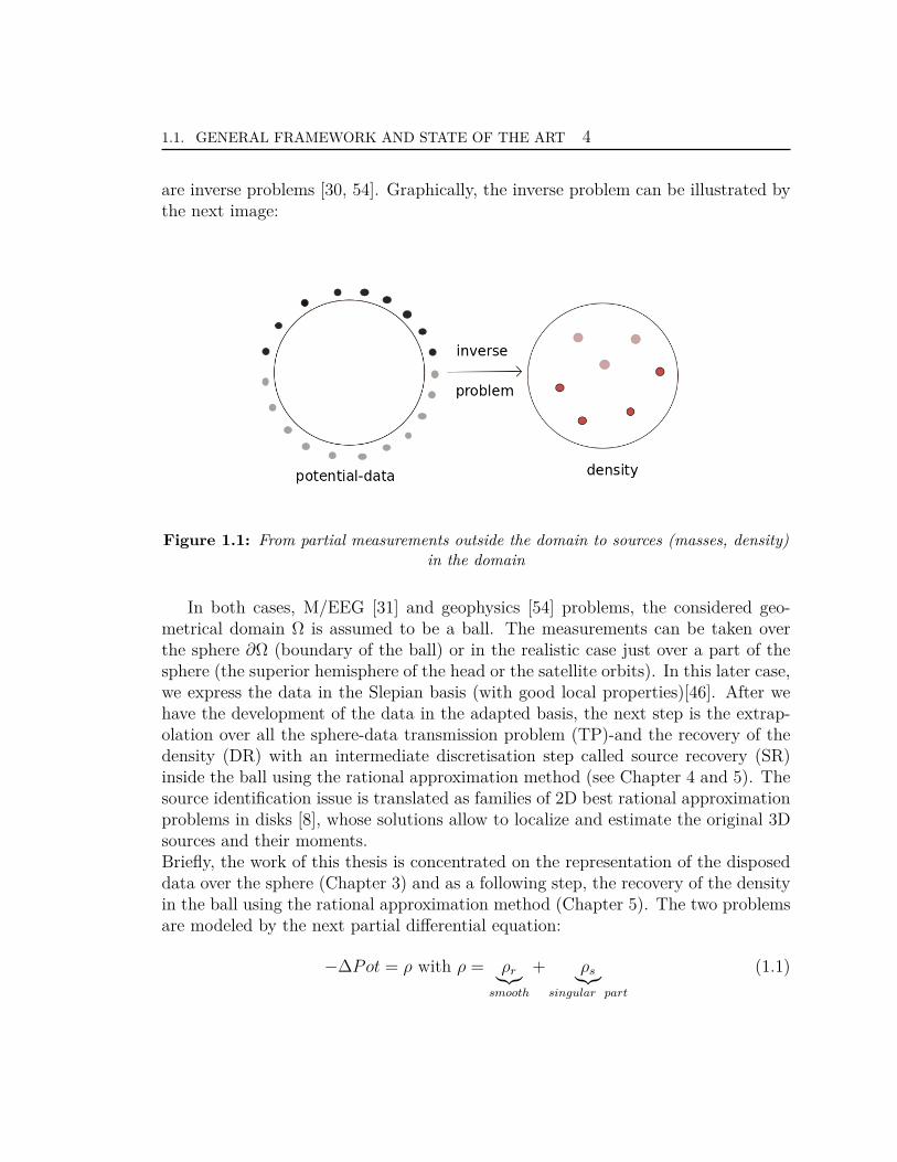
are inverse problems [30, 54]. Graphically, the inverse problem can be illustrated bythe next image:
Figure 1.1: From partial measurements outside the domain to sources (masses, density)in the domain
In both cases, M/EEG [31] and geophysics [54] problems, the considered geo-metrical domain Ω is assumed to be a ball. The measurements can be taken overthe sphere ∂Ω (boundary of the ball) or in the realistic case just over a part of thesphere (the superior hemisphere of the head or the satellite orbits). In this later case,we express the data in the Slepian basis (with good local properties)[46]. After wehave the development of the data in the adapted basis, the next step is the extrap-olation over all the sphere-data transmission problem (TP)-and the recovery of thedensity (DR) with an intermediate discretisation step called source recovery (SR)inside the ball using the rational approximation method (see Chapter 4 and 5). Thesource identification issue is translated as families of 2D best rational approximationproblems in disks [8], whose solutions allow to localize and estimate the original 3Dsources and their moments.Briefly, the work of this thesis is concentrated on the representation of the disposeddata over the sphere (Chapter 3) and as a following step, the recovery of the densityin the ball using the rational approximation method (Chapter 5). The two problemsare modeled by the next partial differential equation:
−∆Pot = ρ with ρ = ρr︸︷︷︸smooth
+ ρs︸︷︷︸singular part
(1.1)
1.2. GEOPHYSICS 5
where Pot can be the electrical, magnetic or gravitational potential and it can bewritten as the convolution between the Green function (see Chapter 2, Section 2.2.1)and the density ρ. The link between these two quantities will be expressed by anoperator called "forward operator" denoted by T :
Pot = G ∗ ρ = Tρ (1.2)
1.2 Geophysics
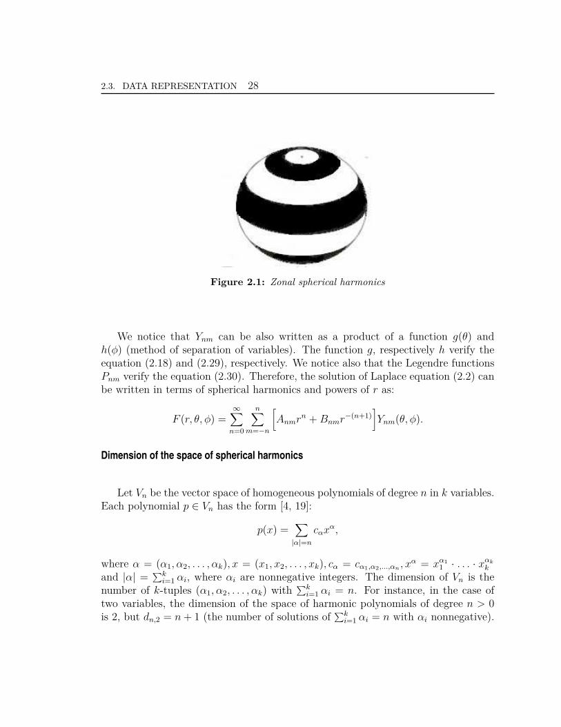
The purpose of this section is to present the physical frame of geophysicalinverse problem. The knowledge of the Earth’s gravity field is essential for manydomains. The gravity field being connected with the internal density of the Earth,it permits to geophysicists to study the structure, the dynamic but also differentphysical properties of the Earth at different scales: from its surface layers to itscenter. One particular equipotential surface, the geoid, which coincides with theaverage of the ocean surfaces, was proposed as the "mathematical figure of theEarth" (C.F. Gauss). It is still frequently considered by many to be the fundamentalsurface of physical geodesy. Referring to the curvature of the interior level surfaces,these change discontinuously with the density. Because the geodetic measurements(theolite measurements, satellite techniques, etc.) are referred to the system ofthe level surface, the geoid plays an important role and thus, we see that one ofthe physical aim is the determination of the level surfaces of the Earth’s gravity field.
The gravity field, at various temporal and space scales, is also used for orbitogra-phy and navigation, locate and characterize different reserves or deposits, to evaluatethe groundwater resource and study polluted sites. The time variations of the gravityfield reflect the mass displacements inside the Earth system, from the Earth’s coreto the top of the atmosphere. Such mass transfer occurs in a wide range of spatialand temporal scales, and they are dominated by the water redistribution related tothe global water cycle in the Earth’s superficial envelopes (atmosphere, oceans, polarice caps, continental hydrology). They also reflect solid Earth deformations such asearthquakes. Measuring and modeling the time variations of the gravity field, andhence of the mass displacements, allow to better understand the dynamical processesand changes in the global Earth system.
1.2. GEOPHYSICS 6
The gravimetry inverse problem
After Isaac Newton, the gravitational potential of the Earth is given by thefollowing formula:
V (X) = G∫∫∫
Ω
ρ(Y )|X − Y |dY ,X ∈ R
3 \ Ω (1.3)
where G is the gravitational constant and ρ is the Earth density.At the exterior of the Earth modeled by Ω, in empty space, the density is zero
and the gravitational potential V satisfies the Laplace equation:
∆V = 0
Inside the Earth Ω, V is solution of the Poisson equation:
∆V = −4πGρ
In what follows, we will suppose 4πG ≃ 1. At the surface of the Earth, we canmeasure the gravitational potential V , but we can also observe measurements ofnormal derivative ∂V
∂n. The normal derivative is the derivative along the outward-
directed surface normal n to the spherical surface of the Earth. According to thesatellite missions CHAMP (Challenging Minisatellite Payload), GRACE (GravityRecovery and Climate Experiment) and GOCE (Gravity Field and Steady-StateOcean Circulation Explorer) we can also have the second order derivative of V(Hessian of V) on satellite orbits. The time-varying component offered by GRACEsatellite improves our knowledge of the data at all spatial scales. Usually, thedata are modeled using a linear combination of spherical harmonics. For regionalmeasurements, local basis functions as Slepian functions, are used.
The direct problem of gravimetry is to find V given the density ρ.
The inverse problem: find the density ρ from boundary measurements of V , ∂V∂n
or Hessian V at ground or on satellite orbits.

1.2. GEOPHYSICS 7
Geometric model of the Earth
Historically, many physicians did scientific observations related to the structureof the Earth.
The first ones that observed the structure multi-shells of the Earth and thedifferent densities for each of them, are Burnet Woodward and Whiston in the XVIIcentury.
A little bit later, Roche proposed 2 shells: a iron kernel of density 7 and a rocksshell of density 3.
In the first decade of the xx century, Lehmann discovered a new structure insidethe kernel. Consequently, the new model is composed by a grain (inner core), acore, a mantle and it is called the Lehmann model.
Bullen proposed in 1936 a concentric model of the Earth with a density whichincrease towards the center (the inner of the Earth).
In 1906, Mohorovici identified a discontinuity between the crust and the mantle.
There are also Gutenberg discontinuity between the lower mantle and outer coreand Lehmann discontinuity between the external and the inner core.
1.2. GEOPHYSICS 8
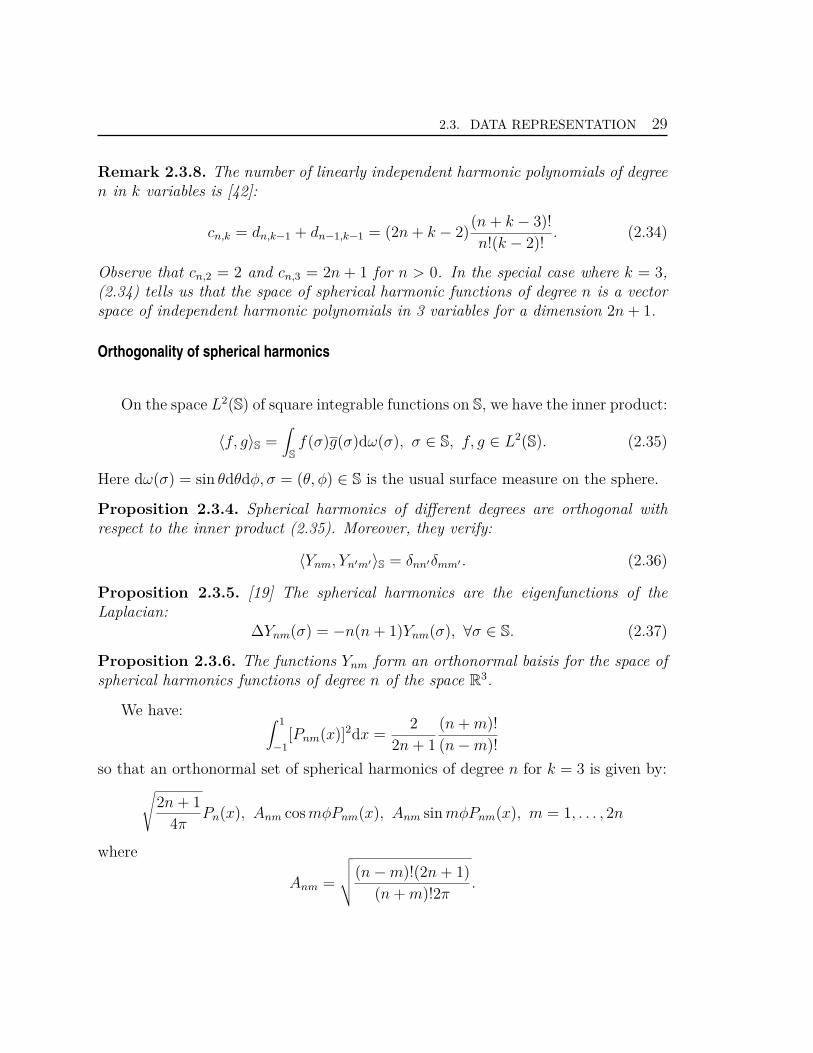
Figure 1.2: Schematic view of the interior of Earth. 1. continental crust - 2. oceaniccrust - 3. upper mantle - 4. lower mantle - 5. outer core - 6. inner core. A: Mo-horovici discontinuity - B: Gutenberg Discontinuity - C: Lehmann discontinuity (Source:http://en.wikipedia.org/wiki )
CRUST
CONTINENTAL
OCEANIC
MOHOROVICI DISCONTINUITY
MANTLESUPERIOR
INFERIOR
GUTENBERG DISCONTINUITY
COREOUTER
INNER
LEHMANN DISCONTINUITY
Figure 1.3: Shells of the Earth and their discontinuities
1.3. M/EEG 9
1.3 M/EEG
The progress of the medical imaging techniques is very important and it is of highutility because it permits to improve continuously the care available for patients.The electroencephalography (EEG) and magnetoencephalography (MEG) are twocomplementary methods which are used for measuring the electric and magneticpotential of the brain [45]. The electromagnetic activity of the brain gives rise to anelectric and magnetic potential which can be measured on the scalp (by electrodes)or outside the head by SQUID (Superconducting Quantum Interference) device.
Magnetoencephalography (MEG) is a technique for measuring the magneticfield induced by the electrical activity of neurons in the brain, classically modeledwith current dipoles [31]. The electroencephalography (EEG) records variations ofelectrical potential at the surface of the scalp.
Both techniques are used for the investigations in neuroscience like the studyand the care of certain cerebral disorders. These two techniques are complementaryand can be measured simultaneously. Nowadays, EEG is relatively inexpen-sive and commonly used. MEG is, comparatively, more expensive because theSQUID device can be used just in a shielded room isolated from the ambientnoise (sensitivity of the device due to the fact that the recorded magnetic poten-tial is of a magnitude of one billion times smaller than the Earth magnetic potential).
Medical engineering aims to localize sources within the brain from measurementsof the electromagnetic potential they produce (the inverse source MEG problem-(IP)). When a limited number of sources are modeled as pointwise and dipolar, ingeneral there are more measurements than unknowns. In the literature of EEG-MEGsource localization problem, there exists several families of methods to solve it, whensources can be modeled as the superposition of a small number of dipoles [45]:
• Dipole fitting methods: minimize a non-convex function, with an outcome thatis unstable with respect to the number of dipoles in the model [18].
• The MUSIC method applies a principal component analysis to the measure-ments, identifies a "noise subspace" and a "signal subspace" and determines thedipole positions by analyzing the signal subspace [41].
1.4. UNIFIED FRAMEWORK 10
• With Beamforming method the sources can be estimated by scanning the regionof interest and by comparing the covariance of the measurement to that of thenoise.
• In this thesis for solving the inverse M/EEG problem, we used the rationalapproximation method in planar sections of the 3D domains and show how thesources are recovered [8]. This method belongs to a new category of sourceestimation algorithms that are grounded in Harmonic Analysis and Best Ap-proximation theory. This method, as well as MUSIC and Beamforming meth-ods, requires no prior information on the number of sources. It works instantby instant and it does not require sources to be decorrelated across time.
Geometric model of the head
The simplified spherical model of the head that can be assumed is the unionof three disjoint homogeneous spherical layers B0, B1, B2, namely the brain, theskull and the scalp. The spheres which separate these volumes are denoted byS0, S1, S2 = S. The main source model available for describing the neuronal activityis the dipolar model described by their number, positions and moments. Forpractical reasons, the data are available only on the outer layer (scalp) by electrodes.For the resolution of the inverse problem, the APICS team uses a technique whichconsists to decompose the 3 dimensional problem in some others 2 dimensionalproblems for which rational approximation techniques are applied (ARL2 theory,for more details see Chapter 5).
For EEG inverse problem we need to pass by a step called «cortical mapping»which allows to propagate the data from the scalp to the interior shell: the brain. InMEG, for the spherical model, this step is not necessary because the data measure-ments depend only on the primary current and not anymore on conductivities [45].
1.4 Unified framework
In practice the measured data (electric, magnetic or gravitational potential)are generally available just over a region Θ ⊂ S or Θ ⊂ SR, R ≥ 1 (the nordhemisphere-M/EEG or satellite orbits-geodesy). Disposing of the partial data, wewant to estimate this data over the whole sphere S, that means to propagate thedata potential from the region Θ of SR to the sphere S (geodesy, MEG) or directly
1.5. OVERVIEW 11
from Θ ⊂ S to whole sphere S. This step called transmission inverse data problem(TP) will be detailled in Chapter 4.
After having the data over the sphere S, we solve the inverse problem (DR)which consists to localize the density inside the ball B. An "intermediate" step tothis problem is the (SR) problem which suppose to approximate the density bypointwise sources and hence to localize the discrete density, as an approximate ofthe continuous density. Source recovery problem from exterior measurements is anill-posed inverse problem in the sense of Hadamard: formally, it is unstable and, inthe distributed source case, non-unique. Constraints, or regularization, are necessaryin order to guarantee a unique and stable solution [29].We say that a problem is not well-posed if one of the next conditions are satisfied:
• it is not solvable (existence of solution);
• it is not uniquely solvable (uniqueness);
• the solution does not depend continuously on the data (stability)
1.5 Overview
Chapter 1 presents an introduction around the geodesy and M/EEG inverseproblems. In Chapter 2 we introduce the background necessary for the study ofthe problems of this thesis. As it was briefly described, the resolution of the inverseproblem (IP) involves the resolution of two problems: the transmission data (TP)and density recovery (DR) problem. In practice, as we know, the data are availablejust on some regions as the north hemisphere of the head (M/EEG) or continents,spherical caps, etc. (geodesy). For this purpose, we will build a new adaptative basison which we express the data. The Chapter 3 provides a new efficient method forbuilding the convenient Slepian basis. The step which consists in passing from thepartial data expressed in the new Slepian basis, to data over the whole sphere S andexpressed in spherical harmonic basis, is called the transmisson data problem (TP).For more details, see Chapter 4. The second step of the (IP) resolution problemis the density recovery (DR) problem, see Chapter 5. In Chapter 6 we presentsome numerical tests to illustrate the sources localization for geodesy and M/EEGproblems when we dispose of partial data.
The main contributions of this work concern:
• the development of a quadrature method for the construction of Slepian basesfunctions on the sphere, together with a study of numerical aspects concerning
1.5. OVERVIEW 12
their use for the representation of potentials on a sphere from partial data (datatransmission);
• the application of best quadratic rational approximation techniques on planarsections (circles) to the extended potential, especially for geophysical issueswhere the gravitational potential is generated by a special piecewise continuousdensity, and in medical engineering, for electroencephalography (and a currentdensity with pointwise dipolar sources). Numerical experiments are providedand discussed (see also [33]).
Chapter2Notations, backgrounds, main problems
In this chapter, we will introduce the main notations and definitions that we usethroughout this thesis and that are necessary for the well comprehension of the nextchapters.
2.1 Notations, definitions
The function space L2(B) represents the set of all square-Lebesgue integrablefunctions from a domain B ⊂ R
n into R. The space L2(B) is equipped with the innerproduct [19]:
〈f, g〉L2(B) :=∫
Bf(x)g(x)dx f, g ∈ L2(B) (2.1)
and the norm ‖f‖L2(B) :=√
〈f, f〉L2(B)
. In this thesis, for simplicity, we will index
the L2(B) norm of a function f just by the domain, i.e. ‖f‖B. The same remark isvalid for the scalar product (2.1), i.e. 〈f, g〉B. For p 6= 2, we denote the Lp norms off by ‖f‖Lp(B).If B = [a, b] and the product is defined in terms of a weighted function ω : [a, b] → R,we note it by 〈f, g〉ω.
2.2 Harmonic functions and elliptic partial derivative equations
A function F is called harmonic function on Rn if it is solution of Laplace equation
[19]:∆F = 0 (2.2)
13
2.2. HARMONIC FUNCTIONS AND ELLIPTIC PARTIAL DERIVATIVE EQUATIONS 14
More precisely, a function is called harmonic in a region B ⊂ Rn if it satisfies
equation of Laplace at every point of B.
Definition 2.2.1. Let L be a linear differential operator of order m with constantcoefficients acting on functions f : B → E of k variables. Thus
(Lf)(x) =∑
|α|≤m
Aα(∂|α|f
∂xα11 . . . ∂xαk
k
)(x)
where E is a given finite-dimensional vector space (typically E = Rp or C
p, p > 1).Here αi, i = 1, 2, . . . , k are nonnegative integers, α = (α1, α1, . . . , αk),|α| = α1 +α2 +. . . αk and Aα are the coefficients. The linear partial differential operator L is saidto be strongly elliptic if for every ξ ∈ S
k−1 and unit vector e ∈ E,
Re〈Pm(ξ)e, e〉E > 0
where Pm is called principal symbol and is given by:
P(ξ) = Pm(ξ) =∑
|α|=m
ξαAα, ξα = ξα
1 . . . ξαk ∈ R
for ξ ∈ Rk.
In this thesis we consider the Laplace elliptic operator of order m = 2 in k = 3variables:
∆f(x) =∂2f
∂x21
+∂2f
∂x22
+∂2f
∂x23
Definition 2.2.2. We recall the Sobolev spaces Wm,p(B),m ∈ Z+, 1 ≤ p ≤ ∞ of a
open domain B:
Wm,p = u ∈ Lp(B) : Dα(u) ∈ Lp(B), for 0 ≤ |α| ≤ m (2.3)
A general stability property for the Neumann problems is given by the followingtheorem:
Theorem 2.2.1. [14] Given a bounded domain B with a C2-boundary Γ, then theNeumann problem:
∆u = f ∈ W r,2(B), r ≥ −1∂nu = g ∈ W s,2(Γ), s ∈ R
(2.4)
2.2. HARMONIC FUNCTIONS AND ELLIPTIC PARTIAL DERIVATIVE EQUATIONS 15
has a solution u ∈ W α,2(B), α = min(r + 2, s+ 32) if and only if:
∫
Γgdγ =
∫
Bfdx
is verified, where dγ is a measure on Γ. If u is a solution, u + c is also a solutionfor ∀c ∈ R. More, we have:
infc∈R
‖u+ c‖W α,2(B) ≤ C(‖f‖W α,2(B) + ‖g‖W s,2(Γ)),
where the constant C depends just on B.
2.2.1 Fundamental solutions and Green functions
The fundamental solution of Laplacian (2.2) in Rn is a distribution En ∈ R
n whichis solution of Poisson equation [19]:
∆En = δ on Rn, (2.5)
with
En(x) = 1n(2−n)ωn
|x|2−n, n > 2, x ∈ Rn;
E2(x) = 12π
log |x|,
with ωn = −(n− 2)σn, where σn is the total surface of the sphere in Rn. En verifies
(2.5) and is the fundamental solution of Laplacian. We introduce also the Greenfunction over the ball B(x0, r0) := Br0 .
G(x, x0) = G(x0, x) =
En(x− x0) − En(x0), n ≥ 3;
12π
log |x−x0|r0
, n = 2.with r0 = |x0|.
Related also to the fundamental solution of Laplacian, we introduce the simple anddouble layer potential. If ϕ ∈ C0(S), then the expression:
u1(x) =∫
S
En(σ − x)ϕ(σ)dω(σ), σ ∈ S
is everywhere defined on Rn and it is called single layer potential [14].
u2(x) =∫
S
∂
∂nEn(σ − x)ϕ(σ)dω(σ) =
1σn
∫
S
Σ(σi − xi)ni(σ)
|σ − x|n ϕ(σ)dω(σ)
It is called double layer potential, where ϕ(σ)dω(σ) is a measure on S, n(σ) is thevector normal to S in σ ∈ S and exterior to B.
2.3. DATA REPRESENTATION 16
Proposition 2.2.1. Given Br0 and u ∈ H(Br0) ∩ C0(Br0). For ∀x ∈ Br0, we havethe Poisson formula:
u(x) =1
r0σn
∫
Sr0
r20 − |x− x0|2
|t− x|n u(t)dwr0(t), (2.6)
where dwr0(t) is a measure on the sphere Sr0 and H(Br0) is the space of the harmonicfunctions on Br0.
2.2.2 Mean-value property
Theorem 2.2.2. [19] Mean-value property for the ball Given Br0, u harmonicand u ∈ L1(Br0), we have:
u(x0) =n
σnrn0
∫
Br0
u(x)dx =n
σnrn−10
∫
B
u(x0 + r0y)dy.
where σn/n is the volume of the unit ball B.
Theorem 2.2.3. [19] Mean-value property for the sphere Given Br0, uharmonic and u ∈ C0(Br0), for every x, we have:
u(x0) =1
σnrn−10
∫
Sr0
u(t)dωr0(t) =1
σnrn−20
∫
S
u(x0 + r0σ)dω(σ).
2.3 Data representation
In solving theoretical and mathematical physical problems, we usually use var-ious special functions. Such kind of problems we can find in connection with heatconduction, propagation of electromagnetic or acoustic waves, etc. Usually, the spe-cial functions are solutions of differential equations. In the following we introduceseveral classes of special functions as: the classical orthogonal polynomials (Jacobi,Laguerre, Hermite, Legendre), spherical harmonics, Bessel and hypergeometric func-tions [4, 52].
2.3. DATA REPRESENTATION 17
2.3.1 Orthogonal polynomials
General properties
In the literature of orthogonal polynomials, there exists many definitions of or-thogonality [4, 52].
Let be [a, b] ⊂ R. The simplest way to say that two polynomials p(x) and q(x)are orthogonal is to write the inner product 〈p, q〉 = 0. The operator 〈·, ·〉 is defined
in terms of the integral of a weighted product 〈p, q〉ω =∫ b
ap(x)q(x)ω(x)dx, with
dω(x) = ω(x)dx, where ω : [a, b] → R is a weight function.
A sequence of polynomials p0, p1, p2, . . . is called sequence of orthogonal polyno-mials if pn is of degree n and all distinct members of the sequence are orthogonalbetween them.
To construct a sequence of orthogonal polynomials, one may use the Gram-Schmidt procedure. For this, we define a projection operator on the polynomials
as: projf (g) =〈f, g〉〈f, f〉f =
b∫af(x)g(x)dx
b∫a(f(x))2dx
f(x), [a, b] ⊂ R. To apply the algorithm, we
define our set of original polynomials g1, g2, . . . , gk by gp(x) = xp, p = 1, . . . , k whichgenerate a sequence of orthogonal polynomials f1, f2, . . . , fk using:
f1 = g1,
f2 = g2 − projf1(g2),
f3 = g3 − projf1(g3) − projf2
(g3),...
fk = gk −k−1∑
j=1
projfj(gk).
Here, the polynomials are supposed to be dense in L2[a, b].
A second method which can be used for the construction of orthogonal polyno-mials is given by the following method of moments:
Let µn =∫Rxndω be the moments of a measure dω. Then the polynomial sequence
defined by:
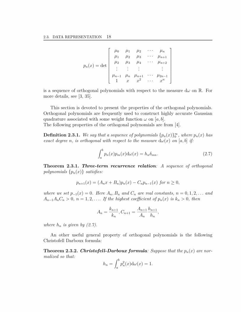
2.3. DATA REPRESENTATION 18
pn(x) = det
µ0 µ1 µ2 · · · µn
µ1 µ2 µ3 · · · µn+1
µ2 µ3 µ4 · · · µn+2...
......
...µn−1 µn µn+1 · · · µ2n−1
1 x x2 · · · xn
is a sequence of orthogonal polynomials with respect to the measure dω on R. Formore details, see [3, 35].
This section is devoted to present the properties of the orthogonal polynomials.Orthogonal polynomials are frequently used to construct highly accurate Gaussianquadrature associated with some weight function ω on [a, b].The following properties of the orthogonal polynomials are from [4].
Definition 2.3.1. We say that a sequence of polynomials pn(x)∞0 , where pn(x) has
exact degree n, is orthogonal with respect to the measure dω(x) on [a, b] if:
∫ b
apn(x)pm(x)dω(x) = hnδmn. (2.7)
Theorem 2.3.1. Three-term recurrence relation: A sequence of orthogonalpolynomials pn(x) satisfies:
pn+1(x) = (Anx+Bn)pn(x) − Cnpn−1(x) for n ≥ 0,
where we set p−1(x) = 0. Here An, Bn and Cn are real constants, n = 0, 1, 2, . . . andAn−1AnCn > 0, n = 1, 2, . . .. If the highest coefficient of pn(x) is kn > 0, then
An =kn+1
kn
, Cn+1 =An+1
An
hn+1
hn
,
where hn is given by (2.7).
An other useful general property of orthogonal polynomials is the followingChristofell Darboux formula:
Theorem 2.3.2. Christofell-Darboux formula: Suppose that the pn(x) are nor-malized so that:
hn =∫ b
ap2
n(x)dω(x) = 1.
2.3. DATA REPRESENTATION 19
Thenn∑
m=0
pm(y)pm(x) =kn
kn+1
pn+1(x)pn(y) − pn+1(y)pn(x)x− y
, (2.8)
where kn is the highest coefficient of pn(x).When hn = 1 and x = y, then:
n∑
k=0
p2k(x) =
kn
kn+1
(p′n+1(x)pn(x) − pn+1(x)p′
n(x))
with p′n+1(x)pn(x) − pn+1(x)p′
n(x) > 0 for all x.
Remark 2.3.1. If hn 6= 1, then (2.8) takes the form:
n∑
m=0
pm(y)pm(x)hm
=kn
kn+1
pn+1(x)pn(y) − pn+1(y)pn(x)(x− y)hn
for x 6= y.
For x = y, we have:
n∑
m=0
(pm(x))2
hm
=kn
hnkn+1
(pn+1(x)pn(x) − pn+1(x)pn(x)).
Remark 2.3.2. Given a sequence of polynomials pn(x) orthogonal with respect toa measure ω(x), the coefficients a(k,m, n) in
pm(x)pn(x) =m+n∑
k=0
a(k,m, n)pk(x)
are given by:
a(k,m, n) =1hk
∫
Ipm(x)pn(x)pk(x)dω(x). (2.9)
A very important class of orthogonal polynomials arises from a differential equa-tion of the form, see [35]:
Q(x) f ′′ + L(x) f ′ + λf = 0, (2.10)
where Q is a given at most quadratic polynomial, and L is a given linear polynomial.The function f , and the constant λ, are to be found. Letting D be the differentialoperator, D(f) = Qf ′′ + Lf ′, and changing the sign of λ, the problem is to findthe eigenvectors (eigenfunctions) f and the corresponding eigenvalues λ, such that fdoes not have singularities and D(f) = λf . The solutions of this differential equation
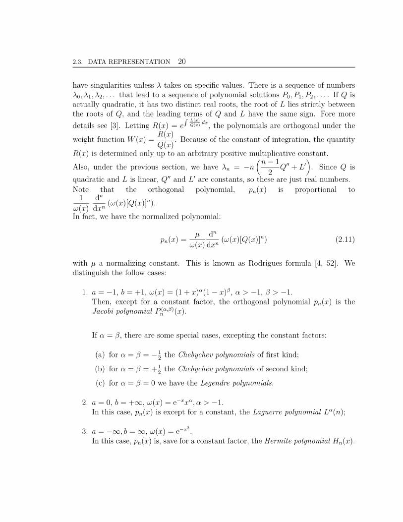
2.3. DATA REPRESENTATION 20
have singularities unless λ takes on specific values. There is a sequence of numbersλ0, λ1, λ2, . . . that lead to a sequence of polynomial solutions P0, P1, P2, . . . . If Q isactually quadratic, it has two distinct real roots, the root of L lies strictly betweenthe roots of Q, and the leading terms of Q and L have the same sign. Fore more
details see [3]. Letting R(x) = e∫
L(x)Q(x)
dx, the polynomials are orthogonal under the
weight function W (x) =R(x)Q(x)
. Because of the constant of integration, the quantity
R(x) is determined only up to an arbitrary positive multiplicative constant.
Also, under the previous section, we have λn = −n(n− 1
2Q′′ + L′
). Since Q is
quadratic and L is linear, Q′′ and L′ are constants, so these are just real numbers.Note that the orthogonal polynomial, pn(x) is proportional to
1ω(x)
dn
dxn(ω(x)[Q(x)]n).
In fact, we have the normalized polynomial:
pn(x) =µ
ω(x)dn
dxn(ω(x)[Q(x)]n) (2.11)
with µ a normalizing constant. This is known as Rodrigues formula [4, 52]. Wedistinguish the follow cases:
1. a = −1, b = +1, ω(x) = (1 + x)α(1 − x)β, α > −1, β > −1.Then, except for a constant factor, the orthogonal polynomial pn(x) is theJacobi polynomial P (α,β)
n (x).
If α = β, there are some special cases, excepting the constant factors:
(a) for α = β = −12
the Chebychev polynomials of first kind;
(b) for α = β = +12
the Chebychev polynomials of second kind;
(c) for α = β = 0 we have the Legendre polynomials.
2. a = 0, b = +∞, ω(x) = e−xxα, α > −1.In this case, pn(x) is except for a constant, the Laguerre polynomial Lα(n);
3. a = −∞, b = ∞, ω(x) = e−x2.
In this case, pn(x) is, save for a constant factor, the Hermite polynomial Hn(x).
2.3. DATA REPRESENTATION 21
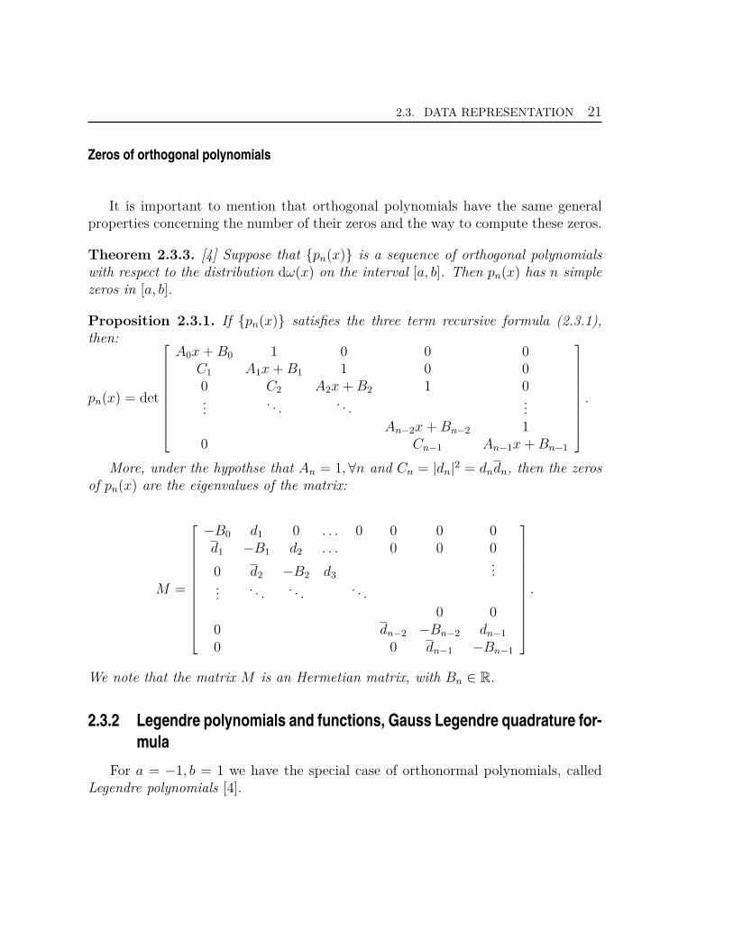
Zeros of orthogonal polynomials
It is important to mention that orthogonal polynomials have the same generalproperties concerning the number of their zeros and the way to compute these zeros.
Theorem 2.3.3. [4] Suppose that pn(x) is a sequence of orthogonal polynomialswith respect to the distribution dω(x) on the interval [a, b]. Then pn(x) has n simplezeros in [a, b].
Proposition 2.3.1. If pn(x) satisfies the three term recursive formula (2.3.1),then:
pn(x) = det
A0x+B0 1 0 0 0C1 A1x+B1 1 0 00 C2 A2x+B2 1 0...
. . . . . ....
An−2x+Bn−2 10 Cn−1 An−1x+Bn−1
.
More, under the hypothse that An = 1,∀n and Cn = |dn|2 = dndn, then the zerosof pn(x) are the eigenvalues of the matrix:
M =
−B0 d1 0 . . . 0 0 0 0d1 −B1 d2 . . . 0 0 0
0 d2 −B2 d3...
.... . . . . . . . .
0 00 dn−2 −Bn−2 dn−1
0 0 dn−1 −Bn−1
.
We note that the matrix M is an Hermetian matrix, with Bn ∈ R.
2.3.2 Legendre polynomials and functions, Gauss Legendre quadrature for-
mula
For a = −1, b = 1 we have the special case of orthonormal polynomials, calledLegendre polynomials [4].

2.3. DATA REPRESENTATION 22
They are given by the formula:
Pn(x) =1
2nn!dn
dxn(x2 − 1)n. (2.12)
The Legendre polynomials form a complete orthogonal set of L2[−1, 1]:∫ 1
−1Pn′(x)Pn(x)dx =
22n+ 1
δn′n. (2.13)
By using Theorem 2.3.2, the relations (2.12) and (2.13), one gets the following re-cursion formula for Legendre polynomials:
Remark 2.3.3. Recursive formula:
P0(x) = 1, P1(x) = x, Pn(x) = −n− 1n
Pn−2(x) +2n− 1n
xPn−1(x). (2.14)
Since the Legendre polynomials form a complete set of L2[−1, 1], any functionf(x) ∈ L2[−1, 1] can be expanded in terms of them:
f(x) =∞∑
n=0
AnPn(x), (2.15)
whereAn =
2n+ 12
∫ 1
−1f(x)Pn(x)dx.
We note that it is possible to compute the successive derivatives of the Legendrepolynomials in an explicit manner. This is done as follows. If P (α,β)
n (x) denote theJacobi polynomials, then we have [4]:
Proposition 2.3.2.
ddxP (α,β)
n (x) =n+ α+ β + 1
2P
(α+1,β+1)n−1 (x).
Consequently, it is easy to see that ∀k, 0 ≤ k ≤ n, we have:
dk
dxkP (α,β)
n (x) =n+ α+ β + 1
2· n+ α+ β + 2
2· . . . · n+ α+ β + k
2P
(α+k,β+k)n−k (x).
If now, we take α = β = 0 one gets the k-derivative of Legendre polynomials Pn infunction of the Jacobi polynomials P
(k,k)n−k :
dk
dxkPn(x) =
n+ 12
· n+ 22
· . . . · n+ k
2P
(k,k)n−k (x). (2.16)
2.3. DATA REPRESENTATION 23
Remark 2.3.4. We denote the Legendre polynomial P (0,0)n (x) by Pn(x).
We introduce Legendre function g(θ) = Pnm(cos θ) as a solution of Legendredifferential equation:
g′′(θ) sin θ + g′(θ) cos θ +[n(n+ 1) sin θ − m2
sin θ
]g(θ) = 0, 0 ≤ θ ≤ π. (2.17)
The subscript n is the degree and the subscript m the order of Pnm.
It is convenient to transform Legendre differential equation (2.17) by the substi-tution x = cos θ ∈ [−1, 1]. We use overbar to denote g as a function of x. Using thisand the substitutions:
g(θ) = g(x),
g′(θ) =dgdθ
=dgdx
dxdθ
= −g′(x) sin θ,
g′′(θ) = g′′(x) sin2 θ − g′(x) cos θ
and then substituting sin2 θ = 1 − x2, we get:
(1 − x2)g′′(x) − 2xg′(x) +[n(n+ 1) − m2
1 − x2
]g(x) = 0, x ∈ [−1, 1]. (2.18)
The Legendre function Pnm(x) is defined by :
Pnm(x) =1
2nn!(1 − x2)
m2
dn+m
dxn+m(x2 − 1)n. (2.19)
For fixed m the functions Pnm(x) form an orthogonal set on the interval −1 ≤ x ≤ 1.They satisfy: ∫ 1
−1Pn′m(x)Pnm(x)dx =
22n+ 1
(n+m)!(n−m)!
δn′n.
We introduce also the normalized associated Legendre functions P nm:
P nm(x) :=
√√√√(2n+ 1)2
(n−m)!(n+m)!
Pnm(x). (2.20)
Remark 2.3.5. For m = 0 in (2.19) we obtain the Legendre polynomials.
In the following, we introduce the addition theorem for Legendre polynomials:
2.3. DATA REPRESENTATION 24
Theorem 2.3.4. Given two points (θ, φ1) and (θ′, φ2) on the unit sphere, we havethe identity [4]:
Pn(cos θ cos θ′ + sin θ sin θ′ cosφ) (2.21)
= Pn(cos θ)Pn(cos θ′) + 2n∑
m=1
(n−m)!(n+m)!
Pnm(cos θ)Pnm(cos θ′) cos(mφ),
where φ = φ1 − φ2 is the spherical distance between (θ, φ1) and (θ′, φ2).
Gaussian quadrature formula
We want to approximate an integral which can not be evaluated exactly.Let us consider Pn(x), n ∈ N a sequence of polynomials orthogonal with respectto measure dω:
∫ b
aPn(x)Pm(x)dω(x) = 0, for m 6= n. (2.22)
Let xj, j = 1, 2, . . . , n denote the zeros of Pn(x).
Theorem 2.3.5. [4] Using the above notations, there are positive numbersλ1, λ2, . . . , λn such that for every polynomial f(x) of degree at most 2n− 1:
∫ b
af(x)dω(x) =
n∑
j=1
λjf(xj). (2.23)
Remark 2.3.6. If f(x) is not a polynomial of degree ≤ 2n − 1, then (2.23) is notexact, but we have an approximation of the integral by the finite left sum.
Remark 2.3.7. Gauss considered the case where dω(x) = dx, Lebesgue measure onR in Theorem 2.3.5. The orthogonal polynomials are then the Legendre polynomialsfor the interval [−1, 1] introduced in Section 2.19.
For an interval [a, b], the integral is approximated by the finite sum:∫ b
af(x)dx ≃
n∑
j=1
λjf(xj),
where the nodes xj are the roots of the Legendre polynomials Pn(x) and the weightsλj are given by the formula:
λj = −an+1
an
1Pn+1(xj)P ′
n(xj), (2.24)
2.3. DATA REPRESENTATION 25
where an denotes the coefficient of xn in Pn.The error of the Gaussian quadrature is given as follows:
∫ b
af(x)dx =
n∑
k=1
λkf(xk) +1a2
n
f (2n)(η)(2n)!
∫ b
aP 2
n(x)dx, a ≤ η ≤ b. (2.25)
2.3.3 Fourier expansion
We identify R2 = (x, y) by the complex space C = z = x+ iy = Reiθ and the
unit circle by eiθ; θ ∈ R.Using the theory of Fourier series, we know that on the unit circle, every f ∈ L2(T)has an expansion of the form:
f(eiθ) =∑
n∈Z
fneinθ =∑
n≥0
fneinθ +∑
n<0
fneinθ = f+(eiθ) + f−(eiθ),
where
f+(z) =∑
n≥0
fnzn,
f−(z) =∑
n<0
fnzn.
For z = reiθ we have:
f+(z) =∑
n≥0
fnrneinθ,
f−(z) =∑
n<0
fnrneinθ =
∑
n>0
f−nr−ne−inθ.
Given f+(z) =∑
n≥0
fnzn and h−(z) =
∑
k>0
hkz−k, the inner product is computed as:
< f+, h− >L2(T)= Re∫ 2π
0f+(eiθ)h−(eiθ)
dθ2π
= Re∑
n,k
fnhk
∫ 2π
0ei(n+k)θ dθ
2π= 0, k > 0, n ≥ 0.
Proposition 2.3.3. Recall briefly that a function f+ is analytic in D if and onlyif f+(z) = u(x, y) + iv(x, y), where u and v are conjugate harmonic functions (theysatisfy the Cauchy-Riemann equations):
∂u
∂x=∂v
∂y,
∂v
∂x= −∂u
∂y,
2.3. DATA REPRESENTATION 26
2.3.4 Hardy spaces
Given f an analytic function on the disk denoted by D, we define:
M2(f, r) =[ 12π
∫ π
−π|f(r expiθ)2|dθ
] 12 and M∞(f, r) = sup
θ|f(reiθ)|,
where r, θ are polar coordinates on D.
‖f‖p = limr→1
Mp(f, r), p = 2,∞.
The Hardy spaces Hp(D), p = 2,∞ are defined being the set of the holomorphicfunctions f on D such that ‖f‖p < ∞ [44].
Definition 2.3.2. H20(D) Hardy space is the orthogonal complementary of H2(D) on
L2(T):L2(T) = H2(D) ⊕H
20(D). (2.26)
For n ≥ 3, the analogous expansion for functions f ∈ L2(S) is got using thespherical harmonics instead of the exponentials einθ, see the following Section.
2.3.5 Spherical harmonics
Laplace equation in spherical coordinates
In spherical coordinates (r, θ, φ), the Laplace equation (2.2) can be written in thefollowing form, see [30]:
1r
∂2
∂r2(rF ) +
1r2 sin θ
∂
∂θ
(sin θ
∂F
∂θ
)+
1r2 sin2 θ
∂2F
∂φ2= 0. (2.27)
The method of separation of variables is used to solve a wide range of linear partialdifferential equations with boundary and initial conditions, such as Laplace equation,heat equation, wave equation, and Helmholtz equation. Using the separation ofvariables, we look for F under the form:
F (r, θ, φ) =U(r)r
P (θ)Q(φ). (2.28)
Substituting (2.28) into (2.27) we get:
Q(φ) = e±imφ, m is a constant
2.3. DATA REPRESENTATION 27
as solution of the equation1Q
d2Q
dφ= −m2. (2.29)
Moreover, P and U satisfy the two differential equations:
1sin θ
ddθ
(sin θ
dPdθ
)+
[n(n+ 1) − m2
sin2 θ
]P = 0 (2.30)
d2U
dr2− n(n+ 1)
r2U = 0 (2.31)
with n(n+ 1) a real constant. The solution of (2.31) is :
U = Anrn+1 +Bnr
−n.
The coefficients An and Bn will be determined from the boundary conditions ofthe problem. In (2.28), the solution of Laplace equation was decomposed into aproduct of factors for three variables r, θ and φ. Now, if we combine the angularfactors, we construct orthonormal functions over the unit sphere. These functionsare called spherical harmonics or tesseral harmonics in older books. The functionsQm(φ) = eimφ, m ∈ Z form a set of orthogonal functions on the interval 0 ≤ φ ≤ 2π.The functions Pnm(cos θ) form a similar set in the index n for each m value on theinterval −1 ≤ cos θ ≤ 1. Therefore their product PnmQm will form an orthogonal seton the surface of the unit sphere in the two indexes n,m. Using the normalizationconstant, given in [42], the suitable normalized spherical harmonics, denoted by Yn,m
are given as follows:
Ynm(θ, φ) =
√√√√2n+ 14π
(n−m)!(n+m)!
Ynm(θ, φ) (2.32)
∫
S
Y 2nm(θ, φ)dω(θ, φ) = 1.
withYnm(θ, φ) = Pnm(cos θ)eimφ, (2.33)
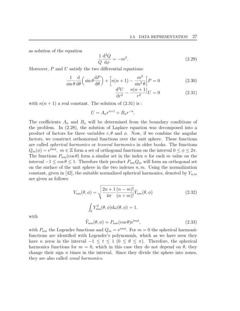
with Pnm the Legendre functions and Qm = eimφ. For m = 0 the spherical harmonicfunctions are identified with Legendre’s polynomials, which as we have seen theyhave n zeros in the interval −1 ≤ t ≤ 1 (0 ≤ θ ≤ π). Therefore, the sphericalharmonics functions for m = 0, which in this case they do not depend on θ, theychange their sign n times in the interval. Since they divide the sphere into zones,they are also called zonal harmonics.
2.3. DATA REPRESENTATION 28
Figure 2.1: Zonal spherical harmonics
We notice that Ynm can be also written as a product of a function g(θ) andh(φ) (method of separation of variables). The function g, respectively h verify theequation (2.18) and (2.29), respectively. We notice also that the Legendre functionsPnm verify the equation (2.30). Therefore, the solution of Laplace equation (2.2) canbe written in terms of spherical harmonics and powers of r as:
F (r, θ, φ) =∞∑
n=0
n∑
m=−n
[Anmr
n +Bnmr−(n+1)
]Ynm(θ, φ).
Dimension of the space of spherical harmonics
Let Vn be the vector space of homogeneous polynomials of degree n in k variables.Each polynomial p ∈ Vn has the form [4, 19]:
p(x) =∑
|α|=n
cαxα,
where α = (α1, α2, . . . , αk), x = (x1, x2, . . . , xk), cα = cα1,α2,...,αn, xα = xα1
1 · . . . · xαk
k
and |α| =∑k
i=1 αi, where αi are nonnegative integers. The dimension of Vn is thenumber of k-tuples (α1, α2, . . . , αk) with
∑ki=1 αi = n. For instance, in the case of
two variables, the dimension of the space of harmonic polynomials of degree n > 0is 2, but dn,2 = n+ 1 (the number of solutions of
∑ki=1 αi = n with αi nonnegative).
2.3. DATA REPRESENTATION 29
Remark 2.3.8. The number of linearly independent harmonic polynomials of degreen in k variables is [42]:
cn,k = dn,k−1 + dn−1,k−1 = (2n+ k − 2)(n+ k − 3)!n!(k − 2)!
. (2.34)
Observe that cn,2 = 2 and cn,3 = 2n + 1 for n > 0. In the special case where k = 3,(2.34) tells us that the space of spherical harmonic functions of degree n is a vectorspace of independent harmonic polynomials in 3 variables for a dimension 2n+ 1.
Orthogonality of spherical harmonics
On the space L2(S) of square integrable functions on S, we have the inner product:
〈f, g〉S =∫
S
f(σ)g(σ)dω(σ), σ ∈ S, f, g ∈ L2(S). (2.35)
Here dω(σ) = sin θdθdφ, σ = (θ, φ) ∈ S is the usual surface measure on the sphere.
Proposition 2.3.4. Spherical harmonics of different degrees are orthogonal withrespect to the inner product (2.35). Moreover, they verify:
〈Ynm, Yn′m′〉S = δnn′δmm′ . (2.36)
Proposition 2.3.5. [19] The spherical harmonics are the eigenfunctions of theLaplacian:
∆Ynm(σ) = −n(n+ 1)Ynm(σ), ∀σ ∈ S. (2.37)
Proposition 2.3.6. The functions Ynm form an orthonormal baisis for the space ofspherical harmonics functions of degree n of the space R
3.
We have: ∫ 1
−1[Pnm(x)]2dx =
22n+ 1
(n+m)!(n−m)!
so that an orthonormal set of spherical harmonics of degree n for k = 3 is given by:√
2n+ 14π
Pn(x), Anm cosmφPnm(x), Anm sinmφPnm(x), m = 1, . . . , 2n
where
Anm =
√√√√(n−m)!(2n+ 1)(n+m)!2π
.
2.3. DATA REPRESENTATION 30
Now take:ξ = (cosα, sinα cosφ1, sinα sinφ1)
andη = (cosβ, sin β cosφ2, sin β sinφ2)
so that (ξ, η) = cosα cos β + sinα sin β cosφ when φ = φ1 − φ2.
Proposition 2.3.7. Addition formula for spherical harmonics:
n∑
m=−n
Ynm(θ, φ)Ynm(θ′, φ′) =2n+ 1
4πPn(cos γ), (2.38)
where cos γ = cos θ cos θ′ +sin θ sin θ′ cosφ is the spherical distance between (θ, φ) and(θ′, φ′).
In the next paragraph we introduce important properties of spherical harmonics:
Proposition 2.3.8. [42] Recursive formula:
cos θ · Ynm =((n+ 1)2 −m2
4(n+ 1)2 − 1
)1/2
Yn+1,m +(n2 −m2
4n2 − 1
)1/2Yn−1,m.
Proposition 2.3.9. [42] Differentiation formula:
∂Ynm(θ, φ)∂θ
= − sin θeimφ
√2π
· dP nm(x)dx
|x=cos θ.
Note that any square-integrable function on the sphere can be expanded in termsof spherical harmonics as:
f(θ, φ) =∞∑
n=0
n∑
m=−n
fnmYn,m(θ, φ), (2.39)
where fnm are the spherical harmonics coefficients associated to Yn,m(θ, φ).These spherical Fourier coefficients fnm can be computed by
fnm = 〈f, Ynm〉S =∫ 2π
0
∫ π
0f(θ, φ)Ynm(θ, φ) sin θdθdφ (2.40)
which by discretization of the integrals is approximately equal to the sum:
D∑
d=1
wdf(θd, φd)Ynm(θd, φd). (2.41)
2.3. DATA REPRESENTATION 31
We note that here the spherical harmonics functions Ynm are normalized, see (2.32).The integral over the sphere ∫
S
f(x)dω(x) (2.42)
is approximately equal to the sum:
D∑
d=1
wdf(θd, φd)Ynm(θd, φd)
by considering the Gauss-Legendre quadrature formula (χS,WS), see [34], whereω(x) is the Lebesgue measure on the sphere and (θd, φd) ∈ χS = θj, j = 0, . . . , S ×φk, k = 0, . . . , 2S + 1- a sampling set of the nodes with
φk = kπS+1
, φk ∈ [0, 2π], S ∈ N.
The θj and φk are called the co-latitudinal and longitudinal nodes, respectively. Forthe co-latitudinal direction we use the Gauss-Legendre quadrature with θj nodes andwj weights which can be obtained as the solution of an eigenvalue problem, see [20],pp. 95. The weights
WS = wd = wj,k, j = 0, . . . , S, k = 0, . . . , 2S + 1
for the entire quadrature formula are then given by:
wj,k =2π
2S + 2wj (2.43)
Comparing with Gaussian quadrature where the nodes are computed as zeros ofLegendre polynomials and the weights are given by 2.43, (see Section 2.3.2), here, thenodes and the weights are given by the couple (χS,WS). Using the Gauss-Legendrequadrature formula, the integral over the sphere:
∫
S
f(x)dw(x) =∫ 2π
0
∫ π
0f(θ, φ) sin θdθdφ
is approximately equal to the double sum:∑
j∈0,...,S
∑
k∈0,...,2S+1
wj,kf(θj, φk).
In the previous integral, we apply a variable change for the interior one and we get:∫ 2π
0
∫ 1
−1f(arccosx, φ)dxdφ (2.44)
2.4. STATEMENT OF THE PROBLEMS 32
which using Gauss-Legendre quadrature formula we get that the initial integral isapproximately equal to:
S∑
j=0
wj
∫ 2π
0f(arccosxj, φ)dφ
The same step is applied for the second integral over [0, 2π] and we get:
S∑
j=0
wj
2S+1∑
k=0
αkf(arccosxj, φk)
Now, we denote the weights for the entire quadrature formula wjαk by wj,k, see(2.43). With this we obtain that the integral on the sphere is approximately equalto:
2S+1∑
k=0
S∑
j=0
2πwj
2S + 2f(arccosxj, φk).
2.4 Statement of the problems
2.4.1 M/EEG
Notations
In this section we introduce the main notations used for the description ofM/EEG problem.For a real value function f(~r), respectively f(~r′), we denote by ∇f , respectively ∇′fthe gradient of f , i.e the vector field whose components are the partial derivativesof f with respect to ~r ∈ R
3, respectively to ~r′-variable.
We denote by:
• ~r the position of the point r in R3;
• ρc(~r, t) the (volumic) charge density at location ~r and time t;
• ~E(~r, t) the electric field vector;
2.4. STATEMENT OF THE PROBLEMS 33
• ~B(~r, t) the magnetic field vector;
• ~J(~r, t) the current density vector.
Maxwell’s equations
Using quasi-static assumptions, Maxwell’s equations lead to a formulation of themagnetic potential ~B as a solution of a differential partial equation.The Maxwell’s equations in vacuum are [30]:
∇ · ~E =ρc
ε0
, ~∇ × ~E = −∂~B∂t, (2.45)
where ε0 ≃ 8.85 10−12Fm−1 is the electrical permittivity of the vacuum and ρc is thetotal charge density:
∇ · ~B = 0, ~∇ × ~B = µo
~J + ε0
∂~E∂t
and µo = 4π10−7Hm−1 is the magnetic permeability. Because the frequencies of theelectromagnetic signals of the brain are very low, the quasi-static approximation ofMaxwell’s equations allows us to neglect the derivatives with respect to time. Withthis assumption, the fourth Maxwell’s equation becomes:
~∇ × ~B = µo~J. (2.46)
Because µo = 0 at the exterior of the head, the curl of the magnetic field is zero:
~∇ × ~B = 0. (2.46′)
Since the curl of the electric field is zero, this field is the gradient of electric potentialU :
~E = −~∇U. (2.47)
Inside the head, the current density ~J, can be decomposed into:-a volumic density ~J
v= σ~E where σ is the head conductivity;
-a primary current ~Jp:
~J = ~Jp
+ σ~E.
2.4. STATEMENT OF THE PROBLEMS 34
Using (2.47), we have:~J = ~J
p − σ~∇U. (2.48)
Using (2.46) and that the curl of the divergence is zero, we have:
∇ · ~J = 0
Thus, using (2.48):∇ · (σ~∇U) = ∇ · ~Jp
.
The primary current generated by N dipolar sources Ck of moments pk is:
~Jp
=N∑
k=1
pk · δCk,
where δCkis the Dirac distribution. Then, we have:
∇ · ~Jp=
N∑
k=1
pk · ∇δCk
and
∇ · (σ~∇U) =N∑
k=1
pk · ∇δCk. (2.49)
Because the sources are localized inside the interior layer (brain), (2.49) becomes:
σ∆U =N∑
k=1
pk.∇δCkin B
σ ∂U∂n |S
= g on S
∆U = 0 in Be.
(2.50)
where, here σ is the brain conductivity.
2.4.2 Geophysics
We recall that inside the Earth, the gravitational potential verifies [54]:
−∆V (X) = ρ(X).
Outside the Earth, the potential verifies the Laplace equation:
∆V (X) = 0.
2.4. STATEMENT OF THE PROBLEMS 35
Now, if we consider a system of several point masses m1,m2, . . . ,mN , the potentialof the system is the sum of each contribution:
V (X) =m1
|X − C1|+
m2
|X − C2|+ . . .+
mN
|X − CN | =N∑
k=1
mk
|X − Ck| .
Here, the density ρ is approximated by a monopolar discrete distribution ρN(X) =∑Nk=1 mkδCk
(X). For (1.3) we assume that point masses are distributed continuouslyover the volume v of the Earth (which is modeled by the unit ball) with densityρ ∈ L2:
ρ =dmdv
with dm an element of the mass and dv an element of volume. In Newton’s integral(1.3), |X −Y | represents the distance between the mass elements dm = ρdv and thepoint Y . Let us consider (x, y, z) the coordinates of the point X and (ξ, η, ζ) thecoordinates of the point Y . Then, the distance |X − Y | becomes:
|X − Y | =√
(x− ξ)2 + (y − η)2 + (z − ζ)2.
The gravitational force F is the gradient of V :
Fx =∂V
∂x, Fy =
∂V
∂y, Fz =
∂V
∂z.
In vector notation, the force vector F is the gradient of the scalar function V :
F = [Fx, Fy, Fz] = gradV.
The disposed measurements can be values of the potential V , of the gravitaionalforce F or of the Hessian of V .
2.4.3 Unified formulation
As we have seen, the both inverse problems are modeled by the partial differentialequation:
−∆Pot = ρ
inside the domain (here, the ball B), and
∆Pot = 0 (2.51)
2.4. STATEMENT OF THE PROBLEMS 36
outside the domain (Be). To underline this commune feature, in the following, we givea mathematical description of the M/EEG and geophysics problems and we introducebriefly the paleomagnetism problem. In all these cases, the direct (forward) problem(FP) and the inverse problem (IP) can be formulated by:
(FP ) :
Tρ = Pot in B;∂P ot∂n |S
= g in S;
and
(IP ) :
∆Pot = ρ in B;∆Pot = 0 in B
e = R \ B;TρN ≃ Pot in S.
The resolution of the inverse problem (IP) consists on two inverse problems: datatransmission problem (TP) and density recovery (DR) by passing by (SR)-sourcerecovery. In general, we dispose of the data just over a region and in this case wepass by the transmission of the data (TP) towards the surface of all the sphere(∂B = S):
(TP): Given values of Pot over a region of S or SR (R > 1) estimate Pot overwhole the sphere S.
The second step which consist in solving the inverse problem is the sourcesrecovery:
(SR): Find the density ρN =∑N
k=1 mkδCkgiven measurements of the discrete
potential PotN .We recall that the problems of our interest are modeled by the next partial differentialequation:
−∆Pot = ρ with ρ = ρr︸︷︷︸smooth
+ ρs︸︷︷︸singular part
(2.52)
In geodesy, we have:ρ = ρr ∈ L2(B) and ρs = 0.
We can dispose of gravimetric measurements ∇V (the gravitational force) on thesurface of the Earth or of satellite measurements of gravitational potential V [1].
Remark 2.4.1. The measurements can be given directly as pointwise values at thesphere surface or as data obtained after the extrapolation step of the transmissionproblem, which is the case that we discuss in this thesis.
2.4. STATEMENT OF THE PROBLEMS 37
In electroencephalography (EEG), we have:
ρs =∑
mk.∇δCkand ρr = 0,
where mk, Ck are the masses of points, respectively the coordinates of these points.The measurements of the electrical potential U or electrical flux ∂nU are taken onthe scalp of the head [8].
In magnetoencephalography (MEG), we have:
ρs =∑
mk.∇δCkand ρr = 0.
Here, mk are the moments of the sources Ck. Radial measurements of the magneticfield ~B are taken at a distance of the head [31]. The magnetic field ~B is the curl ofa vector field ~A called potential vector: ~B = ~∇ × ~A, where ~A verifies ∆ ~A = −µ0
~J,in this case we have a vectorial density, so ρ = −µ0
~J.
In paleomagnetism:
ρs = ∇ · ~M and ρr = 0 where ~M ∈ L1 is a distribution.
The magnetic field of the Earth, ~B, is resumed through the time and it is used todetermine the age of rocks, reconstructions of the deformational histories of parts ofthe crust, etc.

2.4. STATEMENT OF THE PROBLEMS 38
Chapter3Slepian bases on the sphere
In this chapter we present a new basis which is used for the partial representation ofthe data on the sphere. This basis was introduced by Slepian and it was used after,in many domains of applied mathematics. Here we will present two computationmethods already existed in the literature and we introduce one method based on theGauss-Legendre quadrature method.
3.1 Construction of Slepian functions on the sphere
3.1.1 Preliminaries
For the two inverse problems that we considered, the data (the gravitational, electri-cal or magnetic potential) can be measured over the whole sphere or just on a part ofit, as the north hemisphere or a spherical cap, continents, etc. When such a limitedarea is studied, the spherical harmonic basis is prone to error, since it is no longerorthogonal over the partial area. Therefore, the construction of a local spherical har-monic basis that is orthogonal over the studied area of the sphere is required for thestudy of the inverse problem. This issue of finding such a basis was first studied in[2, 36] for an interval of the real line and for balls of Rn. The authors discovered basesof functions (called Slepian functions) with energies concentrated in the consideredregions. This procedure is very useful in several domains of applied mathematics andphysics, notably geophysics [2], cosmology [27] and image processing [15, 48].
39
3.1. CONSTRUCTION OF SLEPIAN FUNCTIONS ON THE SPHERE 40
Bandlimited functions
We recall that any real-valued square-integrable function on the unit sphere canbe expanded as:
g(θ, φ) =∞∑
n=0
n∑
m=−n
gnmYnm(θ, φ) (3.1)
Here, we are interested on the space of square-integrable functions with no powerabove a bandwidth L, i.e g belongs to the space of bandlimited functions denotedby BL with:
BL = g ∈ L2(S)|g =L∑
n=0
n∑
m=−n
gnmYnm
Data concentration within a region of the sphere
Definition 3.1.1. The bandlimited functions g ∈ BL that are optimally concentratedwithin a region Θ of the sphere are called spherical Slepian functions or simply Slepianfunctions, in this thesis.
Slepian functions are those bandlimited functions g ∈ BL for which the concen-tration within Θ is maximum, i.e. to maximize the ratio:
µ =∫
Θ g2(θ, φ)dw
∫Sg2(θ, φ)dω
. (3.2)
These functions are the analogues of one dimensional Slepian’s time-frequencyconcentration problem, see [36], on the surface of the unit sphere. They form anorthonormal basis on the sphere and they are orthogonal over the studied region.Such a basis is a useful tool in data analysis and representation in a variety ofapplications. The spherical Slepian functions can be found by solving an algebraiceigenvalue problem or an integral equation [46], see Section Method 1. In [40], theSlepian functions are seen as a basis for the space of eigenfunctions of an integraloperator, see Definition (3.1.2).
In the case of real line, the computation of one-dimensional Slepian functionswas done using the fact that the differential operator of Sturm Liouville defined onC2([−1, 1]):
L =ddx
(1 − x2)ddx
− c2x2, |x| ≤ 1 (3.3)
3.1. CONSTRUCTION OF SLEPIAN FUNCTIONS ON THE SPHERE 41
obtained by solving the Helmotz equation by the separation of variables method withthe use of prolate spheroidal coordinates, commutes with the integral operator
∫ 1
−1
sin c(x− y)π(x− y)
ψ(y)dy = µψ(x), |x| ≤ 1 (3.4)
where c > 0 is a given real number. The functions ψ are called proloidal sphericalwave functions (PSWF).
Method 1
This method was studied by Simons in [46, 47].In order to maximize the ratio (3.2), we replace g by its bandlimited expansion
and we get:
µ =
L∑
n=0
n∑
m=−n
gnm
L∑
n′=0
n′∑
m′=−n′
Dnm,n′m′gn′m′
L∑
n=0
n∑
m=−n
g2nm
,
where the orthonormality relation of the spherical harmonics is used for the denom-inateur. Define the quantity:
Dnm,n′m′ =∫
ΘYnm(θ, φ)Yn′m′(θ, φ)dω. (3.5)
Now, the maximization problem becomes:
µ =gTDggTg
(3.6)
where D is a (L + 1)2 × (L + 1)2 matrix with elements Dnm,n′m′ and g =(g00, . . . , gnm, . . . , gLL)T the vector of spherical harmonic coefficients associated tothe function g. The matrix D depends on the size of the region Θ and the band-width L.
Every eigenvector gα, α = 1, . . . , (L+1)2 gives rise to an associated eigenfunctiongα ∈ BL. Thanks to the bandwidth L, the eigenfunctions g that are well concentratedwithin the region Θ will have eigenvalues which are near unity, whereas those thatare poorly concentrated will have eigenvalues near zero. Using the index notation,(3.6) is given as follows:
L∑
n=0
n∑
m=−n
Dnm,n′m′gn′m′ = µgnm. (3.7)
3.1. CONSTRUCTION OF SLEPIAN FUNCTIONS ON THE SPHERE 42
If we multiply (3.6) by Ynm and sum over n and m we deduce that the eigenfunctiong satisfies the integral eigenvalue equation of the second kind in Θ:
D(g)(θ, φ) =∫
ΘD((θ, φ), (θ′, φ′))g(θ′, φ′)dw = µg(θ, φ), (θ, φ) ∈ Θ, (3.8)
where D is the integral operator and D is its associated kernel. The kernel D issymmetric and depends on the spherical distance γ between (θ, φ) and (θ′, φ′) givenby cos γ = cos θ′ cos θ + sin θ′ sin θ cos(φ′ − φ):
D((θ, φ), (θ′, φ′)) =L∑
n=0
2n+ 14π
Pn(cos θ′ cos θ + sin θ′ sin θ cos(φ′ − φ))). (3.9)
This method has the drawback to require the computation of the eigenvalues andeigenvectors of an (L + 1)2 × (L + 1)2 order matrix with entries given by (3.5) thatrequires a quadrature method to compute approximate values of these.
Method 2
This method was studied by Miranian in [40]. In Section 3.2 we develop anefficient computational method which uses the Gauss-Legendre quadrature and it isbased on the method of Miranian.
We define the integral operator T over the region Θ ⊂ S:
(T f)(u) =∫
Θ
L∑
n=0
Pn(〈u, u′〉Θ)f(u′)du′ =∫
Θ
L∑
n=0
n∑
m=−n
Ynm(u)Y nm(u′)f(u′)du′, u ∈ Θ
with: ∫ 2π
0
∫ 1
−1Ynm(x, φ)Y nm(x, φ)dxdφ = 1, x = cos θ
where Y nm are the conjugate of (2.32).For a particular region Θ as a polar cap or two symmetrically caps (one at each
pole) defined by Θ : b ≤ cos θ ≤ 1 or 0 ≤ θ ≤ arccos b, 0 ≤ φ ≤ 2π, the SturmLiouville operator S:
S =ddx
[(1 − x2)(b− x)ddx
] − L(L+ 2)x− m2(b− x)1 − x2
(3.10)
defined on the interval [b, 1] commutes with the operator T on the spaces of functionswhose dependence on φ is of the form eimφ. We denote these spaces by Hm with:
3.1. CONSTRUCTION OF SLEPIAN FUNCTIONS ON THE SPHERE 43
Hm = g|g(u) = g(θ, φ) = f(cos θ)eimφ, u ∈ ΘDefinition 3.1.2. The operator Tm is the restriction of the operator T on the spaceHm, m = 0, . . . , L.
When the studied region is not anymore a polar cap, but a region with lesssymmetry, spherical belt bounded by two parallels, etc., with Θ : a ≤ cos θ ≤ b orarccos a ≤ θ ≤ arccos b with θ0 = arccos a, θ1 = arccos b we can always consider theintegral operator Tm, but to get the commuting local operator is not simple.
In the following, let consider a function g ∈ Hm, g(θ, φ) = f(cos θ)eimφ, x = cos θand apply it to the operator T , see [40]:
(Tm)g(u) =∫
Θ(
L∑
l=0
l∑
p=−l
Ylp(u)Y lp(u′))g(u′)du′
=∫
Θ
L∑
l=0
l∑
p=−l
Ylp(x, φ)Y lp(x′, φ′)f(x′)eimφ′
dx′dφ′
=∫ 2π
0
∫ b
a
( L∑
l=0
l∑
p=−l
2l + 14π
(l − p)!(l + p)!
Plp(x)eipφPlp(x′)e−ipφ′
)f(x′)eimφ′
dx′dφ′
=∫ b
a
L∑
l=0
l∑
p=−l
2l + 14π
(l − p)!(l + p)!
Plp(x)Plp(x′)f(x′)(
eipφ∫ 2π
0eiφ′(−p+m)dφ′
)dx′
= eimφ∫ b
a
L∑
l=|m|
2l + 12π
(l − |m|)!(l + |m|)!Plm(x)Plm(x′)f(x′)dx′.
Remark 3.1.1. By applying the operator T to a function g ∈ Hm, the result stillbelongs to Hm.
We denote by Km the kernel of the operator Tm in the space Hm:
Km(x, x′) =L∑
n=|m|
2n+ 12π
(n− |m|)!(n+ |m|)!Pnm(x)Pnm(x′). (3.11)
Here, the problem (3.8) is reduced to the following eigenproblem:∫ b
aKm(x, x′)ψn,m(x′)dx′ = µn(m)ψn,m(x), ∀x ∈ [a, b]. (3.12)
with ψn,m the eigenfunctions of the operator Tm. The rank of Tm is L − |m| + 1and so it admits L − |m| + 1 eigenvalues and L − |m| + 1 eigenfunctions, they areconcentrated in the studied region, the remaining are zero. In the following is giventhe spectral study of the operator Tm, see [40]:
3.1. CONSTRUCTION OF SLEPIAN FUNCTIONS ON THE SPHERE 44
Proposition 3.1.1. Let us consider the finite (L+ 1)2 operator Tm. Then:
• There are L+1 linearly independent orthogonal eigenfunctions of T0 that belongto the space H0; consequently, T0 has only L+ 1 distinct non-zeros eigenvaluesthat correspond to eigenfunctions in H0.
• TheL(L+ 1)
2non zero eigenvalues of Tm have multiplicity 2: in both subspaces
Hm and H−m, Tm has L − m + 1 non-zero distinct eigenvalues, where m =1, . . . , L− 1.
• L − |m| + 1 eigenfunctions of Tm belong to Hm for all |m| = 1, . . . , L − 1 andare orthogonal.
The method used by Simons asks to compute the matrix D whose elements aregiven by (3.5). For L very big, this computation can occupy a lot of memory andtime. In Section 3.2, we give a new practical method for computing the Slepian basisand their associated eigenvalues. This method uses Gauss-Legendre quadrature andit is based on the method proposed by Miranian.
Shifted Legendre polynomials
In the previous paragraph, we saw that the Sturm-Liouville operator S definedon the interval [b, 1] commutes with the operator Tm for those functions which havea dependence on φ of the form eimφ. In order to compute the eigenfunctions of S weuse the shifted Legendre polynomials [40]. Once, we have the eigenfunctions denotedby ψn of the operator S, the Slepian functions are obtained by the multiplicationwith eimφ. The shifted Legendre polynomials are defined to be the solutions of thefollowing second-order differential equation:
(b− x)(1 − x)S ′′n + 2(x− b1)S ′
n − n(n+ 1)Sn = 0 (3.13)
withb1 = (1 + b)/2, b2 = (1 − b)/2.
Proposition 3.1.2. Properties of shifted Legendre polynomials:
Recursion formula:
xSn = b1Sn +b2(n+ 1)2n+ 1
Sn+1 +b2n
2n+ 1Sn−1. (3.14)
3.1. CONSTRUCTION OF SLEPIAN FUNCTIONS ON THE SPHERE 45
Derivative:
(1 − x)(b− x)S ′n = b2
n(n+ 1)2n+ 1
(Sn+1 − Sn−1). (3.15)
Normalized shifted Legendre polynomials:
Sn = Sn
√(2n+ 1)/2b2.
In this case, to solve the problem Sψn = µnψn with m = 0 and m > 0, we usethe shifted Legendre polynomials [40].
For m = 0 the problem is reduced to the problem of computing eigenvectors of acertain symmetric tridiagonal matrix.We have: ( d
dx
[(1 − x2)(b− x)
ddx
]− L(L+ 2)x
)ψn = µnψn. (3.16)
We express ψn in terms of shifted Legendre polynomials:
ψn =∞∑
k=0
ankSk.
In the case m > 0, the problem will be reduced to a generalized matrixeigenproblem Ax = µnBx with A,B two matrices, x their eigenfunctions and µn
their eigenvalues.
3.2. NEW CONSTRUCTIVE METHOD OF SLEPIAN FUNCTIONS ON THE SPHERE 46
3.2 New constructive method of Slepian functions on the
sphere
This method is based on the Gaussian quadrature formula applied to an eigen-problem of the form (3.12) for functions which belong to Hm for x ∈ [a, b].
In this paragraph, we describe our Gaussian quadrature based technique for theaccurate and efficient computation of the Slepian functions on the sphere. Moreover,we will provide the reader with the analysis of this method in computing the valuesof the ψn,m as well as in computing the associated eigenvalues. This method is basedon discretizing (3.12) by using an N -point quadrature formula associated with aLegendre polynomial PN(x) that is an orthogonal family over [a, b] ⊂ [−1, 1]. Hence,(3.12) is approximated by the following eigensystem:
N∑
j=1
wjKm(xi, xj)ψn,m(xj) = µn(m)ψn,m(xi), 1 ≤ i ≤ N. (3.17)
Here, the wi, xi are the weights and the nodes of the N -point Gaussian quadra-ture that are easily computed by the techniques of the paragraph Orthogonality ofspherical harmonics from Chapter 3.
3.2.1 Main results
We recall the substitutions and the notations:
x = cos θ, x′ = cos θ′, xi = cos θi (3.18)
andθ0 = arccos a, θ1 = arccos b. (3.19)
Hence, (3.12) is rewritten as follows:N∑
j=1
wjKm(cos θi, cos θj)ψn,m(cos θj) = µn(m)ψn,m(cos θi), 1 ≤ i ≤ N. (3.20)
We give the two main theorem results of this section:
Theorem 3.2.1. Given an integer 0 ≤ n ≤ L − m and an arbitrary real number0 < ǫ < 1 ∃ N(ǫ, |µn(m)|) ∈ N such that ∀N > N(ǫ, |µn(m)|) we have:
supa≤θ≤b
∣∣∣∣ψn,m(cos θ) − 1µn(m)
N∑
j=1
wjψn,m(cosϕj)Km(cos θ, cosϕj)∣∣∣∣ < ǫ. (3.21)
The wj are the weights associated with the Legendre polynomial PN(x).
3.2. NEW CONSTRUCTIVE METHOD OF SLEPIAN FUNCTIONS ON THE SPHERE 47
The error analysis of our quadrature method for computing the eigenvalues of Tm
is given by the following theorem. We should note that this theorem is an adaptationof a similar theorem given in the case of classical prolate spheroidal wave functionsin [32].
Theorem 3.2.2. Let m > 0 be a positive real number and let consider N an inte-ger with 1 < N ≤ L − m + 1. Let (µi(m))0≤i≤N−1 denote the first N eigenvaluesof the integral operator Tm arranged in decreasing order of their magnitudes. Letx1, . . . , xN ∈ [a, b] and w1, . . . , wN be the N different nodes and weights correspond-ing to the N-th degree Legendre polynomial. Assume that
sup0≤n≤N−1
sup1≤l≤N
|ψn,m(xl) − 1µn(m)
N∑
j=1
wjKm(xl, yj)ψn,m(xj)| ≤ ǫ. (3.22)
Moreover, assume that the matrix B = [ψl−1,m(xj)]1≤l,j≤N is nonsingular. Considerthe matrix AN = [wjKm(xl, yj)]1≤l,j≤N ; then we have:
max0≤j≤N−1
|µj(AN) − µj(Tm)| ≤ǫ√N(L−m+ 1)
π. (3.23)
3.2.2 Bounds of associated Legendre functions and its derivatives
Before to give the proof of these two theorems we introduce the following resultsconcerning the associated Legendre functions.
We consider Pn(R) the set of all algebraic polynomials of degree at most n withreal coefficients. The following theorem is due to A.A. Markov [4]:
Theorem 3.2.3. If p ∈ Pn(R) and ‖p‖[−1,1] := max−1≤t≤1
|p(t)| ≤ 1, then:
‖p′‖[−1,1] ≤ n2. (3.24)
The following theorem gives us a bound for the kth derivative of an algebraicpolynomial:
Theorem 3.2.4. [4] V.A. Markov: For 1 ≤ k ≤ n, if p ∈ Pn(R) and ‖p′‖[−1,1] ≤ 1,we have:
‖p(k)‖[−1,1] ≤ T (k)n (1) · ‖p‖[−1,1] =
n2(n2 − 12) · . . . · (n2 − (k − 1)2)1 · 3 · . . . · (2k − 1)
· ‖p‖[−1,1], (3.25)
where Tn is the nth Chebyshev polynomial of the first kind.
3.2. NEW CONSTRUCTIVE METHOD OF SLEPIAN FUNCTIONS ON THE SPHERE 48
Proposition 3.2.1. For real θ, we have:
|Pn(cos θ)| ≤ 1 (3.26)
and
|P ′n(cos θ)| ≤ 1
2n(n+ 1) (3.27)
from what one may deduce the bound of the kth derivative of Pn:
|P (k)n (cos θ)| ≤ (n+ k)!
(n− k)!k!2k, (3.28)
for 0 ≤ k ≤ n.
Note that in [28], (3.28) is given without proof. To prove this inequality, weproceed as follows:
Proof. We recall the relation (2.16) the derivative of Legendre polynomials Pn infunction of the Jacobi polynomials P (α,β)
n :
dk
dxkPn(x) =
n+ 12
· n+ 22
· . . . · n+ k
2P
(k,k)n−k (x). (3.29)
From (3.29), we have:
|P (k)n (cos θ)| =
∣∣∣n+ 1
2· n+ 2
2· . . . · n+ k
2P
(k,k)n−k (x)
∣∣∣ ≤ (n+ 1)n
2k· max |P (k,k)
n−k (x)|.
or
|P (k)n (cos θ)| =
∣∣∣n+ 1
2· n+ 2
2· . . . · n+ k
2P
(k,k)n−k (x)
∣∣∣ ≤ (n+ k)!2kn!
· max |P (k,k)n−k (x)|.
Proposition 3.2.2.
max−1≤x≤1
|P (α,β)n (x)| =
(q + 1)n
n!, q = max(α, β) ≥ −1/2, (3.30)
where (a)n denotes the shifted factorial defined by:
(a)n = a(a+ 1) . . . (a+ n− 1), for n > 0, (a)0 = 1, a ∈ R.
Remark 3.2.1. We have:
x! =(x+ n)!(x+ 1)n
. (3.31)
3.2. NEW CONSTRUCTIVE METHOD OF SLEPIAN FUNCTIONS ON THE SPHERE 49
Using (3.30),
max−1≤x≤1
|P (k,k)n−k (x)| =
(k + 1)n−k
(n− k)!.
From (3.31),
(k + 1)n−k =(k + n− k)!
k!=n!k!.
Hence,
max−1≤x≤1
|P (k,k)n−k (x)| =
n!k!(n− k)!
.
Therefore,
|P (k)n (cos θ)| ≤ (n+ k)!
2kn!· n!k!(n− k)!
. (3.32)
|P (k)n (cos θ)| ≤ (n+ k)!
2kn!n!
k!(n− k)!=
(n+ k)!(n− k)!k!2k
.
From the definition of Legendre associated functions (2.19) and the previousbound (3.28), it has been mentioned in [28] that:
|Pnm(cos θ)| ≤ |P (m)n (cos θ)| ≤ (n+m)!
(n−m)!m!2m.
A better bound is given in [28] by using the addition theorem for Legendre poly-nomials (see Theorem 2.3.4) and letting θ = θ′ and φ = φ′ in (2.21). Hence, onegets:
1 = Pn(1) = (Pn(cos θ))2 + 2n∑
m=1
(n−m)!(n+m)!
(Pnm(cos θ))2. (3.33)
Because the right side is a sum of positive terms, then each term of (3.33) is boundedby 1. Therefore, we obtain:
|Pnm(cos θ)| ≤[12
(n+m)!(n−m)!
] 12
. (3.34)
Till now we introduced the bounds of Pn and its derivatives. Bounds of theassociated Legendre functions Pnm and its derivatives are obtained in a similar way.Let φ′ = φ and obtain:
Pn(cos(θ− θ′)) = Pn(cos θ)Pn(cos θ′) + 2n∑
m=1
(n−m)!(n+m)!
Pnm(cos θ)Pnm(cos θ′). (3.35)
3.2. NEW CONSTRUCTIVE METHOD OF SLEPIAN FUNCTIONS ON THE SPHERE 50
Now, if we differentiate (3.35) with respect to θ and also θ′ and then set θ = θ′, thisgives:
P ′n(1) =
( ddθPn(cos θ)
)2
+ 2n∑
m=1
(n−m)!(n+m)!
( ddθPnm(cos θ)
)2
. (3.36)
Now, because the right side is a sum of positive terms and the left side is boundedby (3.27) we obtain:
∣∣∣∣ddθPnm(cos θ)
∣∣∣∣ ≤[12n(n+ 1)
(n+m)!2(n−m)!
] 12
(3.37)
for 1 ≤ m ≤ n. Iterating the above process, it is shown in [28] that:
∣∣∣∣( d
dθ
)k
Pnm(cos θ)∣∣∣∣ ≤ Mnk
[(n+m)!(n−m)!
] 12
(3.38)
for 0 ≤ m ≤ n, where M is a constant independent of θ,m and n. To show the nextinequality we use all the previous inequalities.
Proposition 3.2.3. For any integer k ≥ 0, 0 ≤ m ≤ n, arccos a ≤ θ ≤arccos b, arccos a ≤ θ′ ≤ arccos b, we have the following inequality:
∣∣∣∣dkKm(cos θ, cos θ′)
dθk
∣∣∣∣ ≤ 2nk + 2
[(L+ 1)k+2 −mk+1].
Proof. We have:
Km(cos θ, cos θ′) =L∑
n=|m|
2n+ 12π
(n− |m|)!(n+ |m|)!Pnm(cos θ)Pnm(cos θ′),
dkKm(cos θ, cos θ′)dθk
=L∑
n=|m|
2n+ 12π
(n− |m|)!(n+ |m|)!
dkPnm(cos θ)dθk
Pnm(cos θ′).
3.2. NEW CONSTRUCTIVE METHOD OF SLEPIAN FUNCTIONS ON THE SPHERE 51
∣∣∣∣dkKm(cos θ, cos θ′)
dθk
∣∣∣∣ ≤∣∣∣∣
L∑
n=m
2n+ 12π
(n−m)!(n+m)!
dkPnm(cos θ)dθk
Pnm(cos θ′)∣∣∣∣
≤L∑
n=m
2n+ 12π
∣∣∣∣(n−m)!(n+m)!
Mnk[(n+m)!(n−m)!
] 12[12
(n+m)!(n−m)!
] 12∣∣∣∣
= ML∑
n=m
nk(n+
12
)
≤ M[ 1k + 2
((L+ 1)k+2 −mk+2) +1
2(k + 1)((L+ 1)k+1 −mk+1)
]
(3.39)
≤ 2Mk + 2
[(L+ 1)k+2 −mk+1].
Note that to get (3.39), we have used the boundL∑
n=1
nk ≤∫ L+1
1xkdx.
3.2.3 Proof of main results
In the following, we give the proof of our first result.
Proof of Theorem 3.2.1:
Since from (3.12), we have:
∫ θ1
θ0
Km(cos θ, cosϕ)ψn,m(cosϕ) sinϕdϕ = µn(m)ψn,m(cos θ). (3.40)
From (3.40), we get the relation:
ψn,m(cos θ) =1
µn(m)
∫ θ1
θ0
Km(cos θ, cosϕ)ψn,m(cosϕ) sinϕdϕ (3.41)
=1
(µn(m))2
∫ θ1
θ0
∫ θ1
θ0
Km(cos θ, cosϕ)Km(cosϕ, cos θ′
)ψn,m(cos θ′
) sin θ′
sinϕdθ′
dϕ.
By using (3.41), to write ψn,m(cosϕj), one gets:
3.2. NEW CONSTRUCTIVE METHOD OF SLEPIAN FUNCTIONS ON THE SPHERE 52
1µn(m)
N∑
j=1
wjψn,m(cosϕj)K(m, cos θ, cosϕj)
=1
(µn(m))2
∫ θ1
θ0
N∑
j=1
wjKm(cos θ, cosϕj)Km(cosϕj, cos θ′)ψn,m(cos θ′
) sin θ′dθ′.
Hence, one gets:
∣∣∣∣ψn,m(cos θ) − 1µn(m)
N∑
j=1
wjψn,m(cosϕj)Km(cos θ, cosϕj)∣∣∣∣
≤ 1|µn(m)|2
∫ θ1
θ0
∣∣∣∣∫ θ1
θ0
Km(cos θ, cosϕ)Km(cosϕ, cos θ′
) sinϕdϕ
−N∑
j=1
wjKm(cos θ, cosϕj)Km(cosϕj, cos θ′
)∣∣∣∣ · |ψn,m(cos θ
′
)| sin θ′
dθ′
.
We denote by I the interior of the first integral:
I =∫ θ1
θ0
Km(cos θ, cosϕ)Km(cosϕ, cos θ′
)d cosϕ−N∑
j=1
wjKm(cos θ, cosϕj)Km(cosϕj, cos θ′
).
We apply the Gaussian quadrature error given via the following equation:
∫ b
af(x)dx =
n∑
k=1
wkf(xk) +1a2
n
f (2n)(η)(2n)!
∫ b
aP 2
n(x)dx, a ≤ η ≤ b. (3.42)
In terms of the substitutions (3.19) and in the case where f(x) is substituted with
Km(cos θ, cosϕ)Km(cosϕ, cos θ′
)
and (3.42) is rewritten as follows:∫ θ1
θ0
Km(cos θ, cosϕ)Km(cosϕ, cos θ′
) sinϕdϕ
=n∑
k=1
wkKm(cos θ, cosϕk)Km(cosϕk, cos θ′
)
+1
a2N(2N)!
∂2N
∂ϕ2NKm(cos θ, cosϕ)Km(cosϕ, cos θ
′
)∣∣∣∣ϕ=η
·∫ θ1
θ0
P 2n(cos θ) sin θdθ.
3.2. NEW CONSTRUCTIVE METHOD OF SLEPIAN FUNCTIONS ON THE SPHERE 53
with θ0 ≤ η ≤ θ1.
To abreviate the notation, we will write:
Km(θ, ϕ, θ) = Km(cos θ, cosϕ)Km(cosϕ, cos θ′
).
For computing the 2Nth derivative of Km(θ, ϕ, θ), we apply the Leibnitz formula:
d2N
dϕ2N[Km(θ, ϕ, θ′)] =
k∑
l=0
C lk
dl
dϕl[Km(cos θ, cosϕ)]
dk−l
dϕk−l[Km(cosϕ, cos θ
′
)].
For k = 2N and using the fact that the kernel Km is symmetric, we obtain:
d2N
dϕ2N[Km(cos θ, cosϕ)Km(cosϕ, cos θ
′
)] ≤ M22N∑
l=0
C l2N
L∑
n=m
n2N(n+
12
)2
= M22N∑
l=0
C l2N
L∑
n=m
(n2N+2 + n2N+1 +n2N
4) ≤ M2 · 4N
[ 12N + 3
((L+ 1)2N+3 −m2N+3)
+1
2N + 2((L+ 1)2N+2 −m2N+2) +
14(2N + 1)
((L+ 1)2N+1 −m2N+1)]
≤ M24N42N + 3
[(L+ 1)2N+3 −m2N+1
]=
(2N+1M)2
2N + 3
[(L+ 1)2N+3 −m2N+1
]= CM,N,L,
where2N∑
l=0
C l2N =
(2N)!l!(2N − l)!
= 22N .
I ≤ 1|µn(m)|2 · CM,N,L
(2N)!a2N
‖ψn,m‖2,[a,b] ≤ 1|µn(m)|2
CM,N,L
(2N)!a2N
|µn(m)| =CM,N,L
(2N)!a2N
1|µn(m)|
with:
aN =(2N)!hN
N !, hN =
√2N + 1
(b− a)N+ 12N !
. (3.43)
We call the Weyl’s perturbation theorem used in error analysis study:
Theorem 3.2.5. Let A and B be two hermitian matrices of order n, where ‖ · ‖ isthe norm defined on the space n× n size of matrices M(Rn × R
n). Then:
max0≤j≤n−1
|µj(A) − µj(B)| ≤ ‖A−B‖.
Here, µj are the eigenvalues of A and B, respectively and
3.2. NEW CONSTRUCTIVE METHOD OF SLEPIAN FUNCTIONS ON THE SPHERE 54
|µ0(A)| ≥ |µ1(A)| ≥ . . . |µn−1(A)|, |µ0(B)| ≥ |µ1(B)| ≥ . . . |µn−1(B)|
are their rearrangements.
We give the proof of the second result.
Proof of Theorem 3.2.2:
We build the Hilbert space EN defined by
EN = Spanψ0,m, ψ1,m, . . . , ψN−1,m.
Let TN,m, TN,m : EN → RN be two operators defined by:
TN,m(f) =[ ∫ b
aKm(xj, y)f(y)dy
]t
1≤j≤N.
TN,m(f) =[ N∑
k=1
wkKm(xj, yk)f(yk)]t
1≤j≤N.
TN,m, TN,m We have:
TN,m(ψi,m) = µi(m)Ψi, 0 ≤ i ≤ N − 1,
where Ψi = [ψi,m(x1), . . . , ψi,m(xN)]t ∈ RN . Note that, by assumption,
B = Ψ0,Ψ1, . . . ,ΨN−1
is a basis of RN . Moreover, since:
TN,m(ψl,m) =[ N∑
k=1
wkKm(xj, xk)ψl,m(xk)]t
1≤j≤N= ANψl,m, 0 ≤ l ≤ N − 1,
where AN is the matrix representation of TN,m. Then, we have:
‖TN,m − TN,m‖2 ≤N−1∑
l=0
|µl(m)|2 ·N∑
j=1
[ψl,m(xj) − 1
µl(m)
N∑
k=1
wkKm(xj, xk)ψl,m(xk)]2
≤∑
0≤l≤N−1
Nǫ2|µl(m)|2 ≤ Nǫ2∑
l≥0
|µl(m)|2. (3.44)
3.3. NUMERICAL ILLUSTRATIONS 55
We compute∑
l≥0
|µl(m)|2:
‖Tm‖2 =∑
l≥0
|µl(m)|2 =∫ b
a
∫ b
a|Km(x, y)|2dxdy,
=∫ b
a
∫ b
a
L∑
n=m
L∑
p=m
2n+ 12π
(n−m)!(n+m)!
Pnm(x)Pnm(y)2p+ 1
2π(p−m)!(p+m)!
Ppm(x)Ppm(y)dxdy,
=L∑
n,p=m
(2n+ 1)(2p+ 1)4π2
∫ b
a(Pnm(x)Ppm(x))dx
∫ b
a(Pnm(y)Ppm(y))dy
≤L∑
n=m
(2n+ 1)2
4π2
∫ 1
−1(Pnm(x))2)dx
∫ 1
−1(Pnm(y))2)dy
=L∑
n=m
(2n+ 1)2
4π2
22
(2n+ 1)2=L−m+ 1
π2,
then we have:
‖TN,m − TN,m‖2 ≤ Nǫ2(L−m+ 1)π2
.
Becauseµ(TN,m) = µ(AN)
andµj(TN,m) = |µj(m)|, j = 0, . . . , N − 1,
then, by using Weyl’s perturbation theorem and the previous inequality, we get:
max1≤j≤N
|µj(TN,m) − µj(TN,m)| = max1≤j≤N
∣∣∣∣|µj(m)| − µj(AN)∣∣∣∣
≤ ‖TN,m − TN,m‖ ≤ǫ√N(L−m+ 1)
π
3.3 Numerical illustrations
To compute the Slepian functions by using Gauss-Legendre quadrature, we needthe weights and the nodes in that we evaluate them. An example of the computednodes and weights of the Gauss-Legendre quadrature over the sphere are given inAnnexe (see Fig.1). In the next figure we show the distribution of these nodes thatwe took over the sphere and in which the potential is computed:
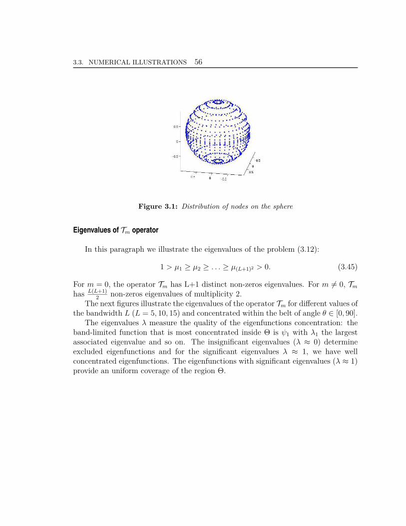
3.3. NUMERICAL ILLUSTRATIONS 56
Figure 3.1: Distribution of nodes on the sphere
Eigenvalues of Tm operator
In this paragraph we illustrate the eigenvalues of the problem (3.12):
1 > µ1 ≥ µ2 ≥ . . . ≥ µ(L+1)2 > 0. (3.45)
For m = 0, the operator Tm has L+1 distinct non-zeros eigenvalues. For m 6= 0, Tm
has L(L+1)2
non-zeros eigenvalues of multiplicity 2.The next figures illustrate the eigenvalues of the operator Tm for different values of
the bandwidth L (L = 5, 10, 15) and concentrated within the belt of angle θ ∈ [0, 90].The eigenvalues λ measure the quality of the eigenfunctions concentration: the
band-limited function that is most concentrated inside Θ is ψ1 with λ1 the largestassociated eigenvalue and so on. The insignificant eigenvalues (λ ≈ 0) determineexcluded eigenfunctions and for the significant eigenvalues λ ≈ 1, we have wellconcentrated eigenfunctions. The eigenfunctions with significant eigenvalues (λ ≈ 1)provide an uniform coverage of the region Θ.
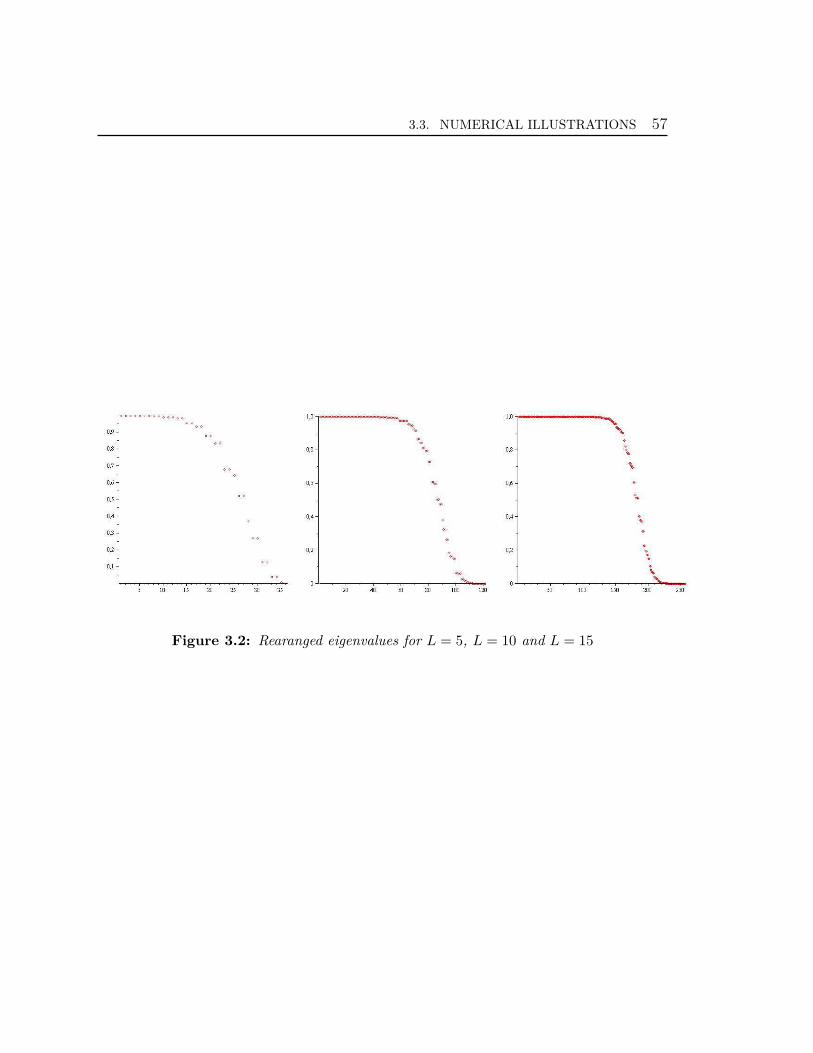
3.3. NUMERICAL ILLUSTRATIONS 57
Figure 3.2: Rearanged eigenvalues for L = 5, L = 10 and L = 15
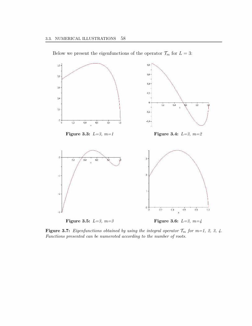
3.3. NUMERICAL ILLUSTRATIONS 58
Below we present the eigenfunctions of the operator Tm for L = 3:
Figure 3.3: L=3, m=1 Figure 3.4: L=3, m=2
Figure 3.5: L=3, m=3 Figure 3.6: L=3, m=4
Figure 3.7: Eigenfunctions obtained by using the integral operator Tm for m=1, 2, 3, 4.Functions presented can be numeroted according to the number of roots.
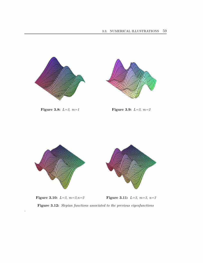
3.3. NUMERICAL ILLUSTRATIONS 59
Figure 3.8: L=3, m=1 Figure 3.9: L=3, m=2
Figure 3.10: L=3, m=3,n=2 Figure 3.11: L=3, m=3, n=3
Figure 3.12: Slepian functions associated to the previous eigenfunctions
.

3.3. NUMERICAL ILLUSTRATIONS 60
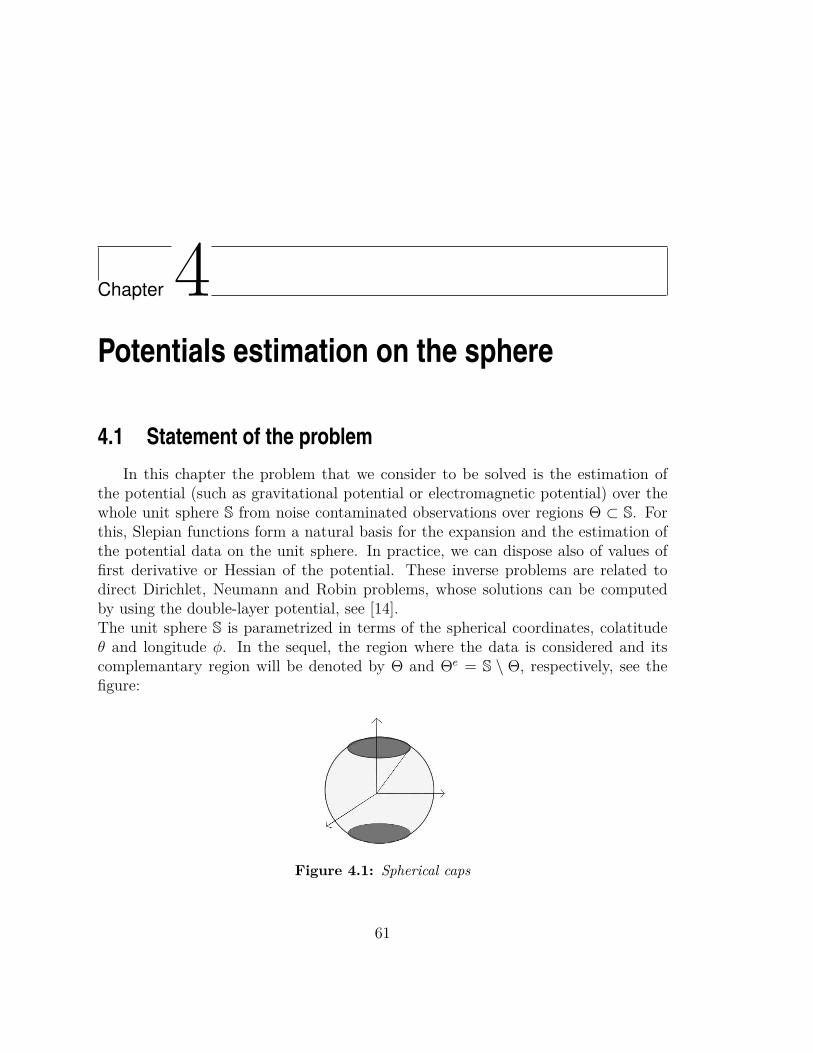
Chapter4Potentials estimation on the sphere
4.1 Statement of the problem
In this chapter the problem that we consider to be solved is the estimation ofthe potential (such as gravitational potential or electromagnetic potential) over thewhole unit sphere S from noise contaminated observations over regions Θ ⊂ S. Forthis, Slepian functions form a natural basis for the expansion and the estimation ofthe potential data on the unit sphere. In practice, we can dispose also of values offirst derivative or Hessian of the potential. These inverse problems are related todirect Dirichlet, Neumann and Robin problems, whose solutions can be computedby using the double-layer potential, see [14].The unit sphere S is parametrized in terms of the spherical coordinates, colatitudeθ and longitude φ. In the sequel, the region where the data is considered and itscomplemantary region will be denoted by Θ and Θe = S \ Θ, respectively, see thefigure:
Figure 4.1: Spherical caps
61
4.2. NOISY MEASUREMENTS 62
4.2 Noisy measurements
We consider the signal [46]:
s(σ) =L∑
nm
snmYnm(σ)︸ ︷︷ ︸
bandlimited component
+∞∑
nm>L
snmYnm(σ)
︸ ︷︷ ︸non bandlimited component
σ = (θ, φ) ∈ S (4.1)
with the coefficients of the signal spherical harmonic expansion given by:
snm =∫
S
s(σ)Ynm(σ)dω(σ). (4.2)
The data over the covered region Θ is given by (4.1), but they are contamined bynoise. Thus, a satellites measures:
d(σ) = s(σ) + n(σ), if σ ∈ Θ,Θ ⊂ S (4.3)
We assume that the noise is modelled by a function n ∈ L2(Θ) with the norm ‖n‖Θ
small.
4.3 Signal field estimation
Being given the noisy data d taken by the satellites over an incomplete regionΘ, we look to estimate the signal s, that gives rise to these observations. Althoughthe signal has an infinite bandwidth, we will be able, practically, only to makebandlimited estimates of it, which we denote by s. The limitation to the bandwidthL as well as the spatial restriction of the observations to the region Θ motivates toseek an estimate in terms of Slepian basis that are well concentrated in the consideredregion, rather than using the non-localized spherical harmonics Ynm. In this manner,the signal is given by:
s(σ) =(L+1)2∑
α
sαgα(σ) +∞∑
nm>L
snmYnm(σ), σ = (θ, φ) ∈ S
whereas the estimated signal s(σ) is given on S by:
s(σ) =L∑
nm
snmYnm(σ) =(L+1)2∑
α=1
sαgα(σ), (4.4)
4.3. SIGNAL FIELD ESTIMATION 63
where (gα)1≤α≤(L+1)2 , α = α(n,m) are the Slepian functions on the sphere S thatare concentrated on the region Θ and associated with the bandwidth L > 0, see(3.7) (after the computation method used by Miranian, we have ψn,m(θ) sinmφ,ψn,m(θ) cosmφ, 0 ≤ n ≤ L,m ≤ n ≤ L for Slepian functions).
The Slepian functions gα verify:
gα(σ) =L∑
nm
gα,nmYnm(σ), σ ∈ S (4.5)
gα,nm =∫
S
gα(σ)Ynm(σ)dω(σ). (4.6)
Using (4.1) and (4.6) we get:
snm =(L+1)2∑
α=1
gα,nmsα (4.7)
and
sα =L∑
nm
gα,nmsnm. (4.8)
The Slepian functions g1(σ), . . . , g(L+1)2(σ) are defined on the part Θ of the unitsphere S.
Now, if we index gα in terms of an index β(n,m), between α and β there existsa bijective mapping such that α = β(n,m).Using the Miranian computational method, the Slepian functions are given by
ψLβ(n,m)(θ)(ηn,m cosmφ+ (1 − ηn,m) sinmφ).
where
ηn,m =
1 if 1 ≤ n ≤ (L−m+ 1)0 if L−m+ 2 ≤ n ≤ 2(L−m+ 1)
(L+1)2∑
α=1
sαgα =L+1∑
n=0
sLβ(n,0)ψ
Lβ(n,0)(θ) cosmφ
+L∑
m=1
2(L−m+1)∑
n=1
sLβ(n,m)ψ
Lβ(n,m)(θ)(ηn,m cosmφ+ (1 − ηn,m) sinmφ)
4.3. SIGNAL FIELD ESTIMATION 64
with
βn,m =
n if 1 ≤ n ≤ (L+ 1),m = 0(L+ 1) + (m− 1)(2L− (m− 2)) + n if 1 ≤ n ≤ 2(L−m+ 1), 1 ≤ m ≤ L.
The coefficients of the Slepian functions can be computed by:
sLβ(n,m) = 〈s, ψL
β(n,m)(θ)(ηn,m cosmφ+ (1 − ηn,m) sinmφ)〉Θ. (4.9)
For simplicity, in what follows, the Slepian functions ψLβ(n,m)(θ)(ηn,m cosmφ + (1 −
ηn,m) sinmφ) will be denoted by Ψn,m(θ, φ) or Ψn,m(σ). The normalized Slepianfunctions are denoted by Ψn,m. They are orthonormal over the sphere and orthogonalover the region Θ: ∫
S
Ψn,m(σ)Ψn′,m′(σ)dω(σ) = δn,n′δm,m′ (4.10)
∫
ΘΨn,m(σ)Ψn′,m′(σ)dω(σ) = µnmδn,n′δm,m′ (4.11)
The inverse problem which consists to estimate the signal s over the whole sphere S
from measurements of the noisy data d on the region Θ, becomes to minimize:∫
Θ(s(σ) − d(σ))2dω(σ). (4.12)
In [46], the estimate of the field coefficients is given by:
snm =L∑
n′m′
D−1nm,n′m′
∫
Θd(σ)Yn′,m′(σ)dω(σ), (4.13)
where Dnm,n′m′ is given by (3.5).Because D composed by the elements Dnm,n′m′ , see (3.5) has a low condition number,finding a stable inverse D−1 is problematic, hence the problem is ill-conditioned. Tostabilize the solution it was included a weighted norm to the minimization problem(4.12): ∫
Θ(s− d(σ))2dω(σ) + η
∫
Θes2dω(σ), (4.14)
where η > 0 is a damping parameter.Involving (4.4) and (3.5), we get:
snm =L∑
n′m′
(Dnm,n′m′ + ηDnm,n′m′)−1 ×∫
Θd(σ)Yn′,m′(σ)dω(σ) (4.15)
4.3. SIGNAL FIELD ESTIMATION 65
withDnm,n′m′ =
∫
ΘeYnmYn′,m′dw = δnn′δmm′ −Dnm,n′m′ . (4.16)
The relation (4.15) holds for n ≤ L, since, when n > L, no estimate is available,snm = 0. The case where n = 1, for which D + D = I, the identity matrix, wastreated by Sneeuw and Gelderen [50].
By substituting the equation (4.3) and using (4.4), (3.5), the integral over thedata in (4.15) becomes:
∫
Θd(σ)Yn′,m′(σ)dω(σ) =
∑
n′m′
Dnm,n′m′sn′m′ +∫
Θn(σ)Ynm(σ)dω(σ). (4.17)
After we compute∫
Θd(σ)Yn′,m′(σ)dω(σ), we get the coefficients snm and consequently
the signal s. Now, if we use the Slepian expansion of s:
s =(L+1)2∑
α=1
sαgα, (4.18)
the coefficients sα are computed according to (4.8). A Slepian basis expansion of theobservations, combining (4.1), (4.3), (4.4), is given by:
d(σ) =(L+1)2∑
α=1
sαgα +∞∑
nm>L
snmYnm(σ) + n(σ). (4.19)
This equation allows us to find an alternative expression for the data integral (4.17),for which we also use (4.5), (3.5) and (3.6):
∫
Θd(σ)Ynmdω(σ) =
(L+1)2∑
α=1
gα,nm(µαsα +∫
Θngαdω(σ)) +
∞∑
n′m′>L
Dnm,n′m′sn′m′ . (4.20)
where µα are the eigenvalues associated to the eigenfunctions gα, see (3.6). Inserting(4.7), (4.14), (4.20) into (4.4), we get the following formula for the computation ofs:
s(σ) =(L+1)2∑
α=1
µ∗α(η)gα(σ) ×
(µαsα +
∫
Θn(σ)gαdω +
∞∑
nm>L
Dnm,n′m′sn′m′
)
withµ∗
α(η) = [µα + η(1 − µα)]−1.
4.4. BANDLIMITED SIGNALS EXPANSION 66
Remark 4.3.1. In practice, the data is measured by satellites at an altitude a fromthe unit sphere S. In this case, instead to consider the data on S it can be supposedknown at the surface of S1+a, R = 1 + a.
Then, at the altitude a above the unit sphere, the signal is given by:
su(σ) =L∑
nm
sunmYnm(σ) +
∞∑
nm>L
sunmYnm(σ), (4.21)
wheresu
nm = (1 + a)−(n+1)snm. (4.22)
where the index u denotes the upward component.
Remark 4.3.2. The estimation problem (4.14) can be also formulated in terms ofbest constrained approximation problems (BEP), see [5].
4.4 Bandlimited signals expansion
Given sL ∈ BL a bandlimited function on the sphere, we have that sL(σ) has thefollowing Slepian functions expansion on the region Θ and the sphere S:
On the sphere S:
sL(σ) =L∑
m=0
2(L−m+1)∑
n=1
anmΨn,m(σ) =L∑
m=0
2(L−m+1)∑
n=1
anm√µnmΨn,m(σ), (4.23)
where Ψn,m(σ) are the normalized Slepian functions introduced in (4.9).Using (4.10) and (4.11), we have:
∫
Θ|Ψn,m(σ)|2dω(σ) = 1 (4.24)
and ∫
S
|Ψn,m(σ)|2dω(σ) =1µnm
, (4.25)
where the µnm are the eigenvalues associated to the eigenfunctions of the operator Tm.
On the region Θ:
sL(σ) =L∑
m=0
2(L−m+1)∑
n=1
bnmΨn,m(σ), (4.26)

4.4. BANDLIMITED SIGNALS EXPANSION 67
Ψn,m(σ) is a basis for L2(R) ∩BL, where:
BL = s ∈ L2(S), s is an L− bandlimited function. (4.27)
On the region Θ, the equations (4.23) and (4.26) hold simultaneously, that is:
bn,m =√µnmanm, 1 ≤ n ≤ 2(L−m+ 1). (4.28)
Moreover, we have from (4.23):
‖sL‖2S
=L∑
m=0
2(L−m+1)∑
n=1
|anm|2. (4.29)
Hence,|bnm|õnm
= |anm| ≤ ‖sL‖S,∀n,m. (4.30)
By combining, (4.28) and (4.30), we conclude that the |bnm|2 have the same decayas the sequence of eigenvalues µnm, 0 ≤ m ≤ L, 1 ≤ n ≤ 2(L − m + 1). They havealso a faster decay than the spherical harmonic coefficients.
Example:
In this example, we consider a particular signal, the gravitational potential V ,defined on S by:
V (X) =N∑
k=1
mk
|X − Sk| , (4.31)
where Sk are monopolar sources and mk their masses. We define also the regionΘ = (θ, φ), θ ∈ [0, 90], φ ∈ [0, 2π]. Then, the first spherical harmonic coefficientsexpansion of V and the corresponding Slepian functions expansion coefficients aregiven by the next table. The gravitational potential V is supposed to be generatedby the monopolar source S = (−0.06, 0.42, 0.25) of masse m = 0.6.
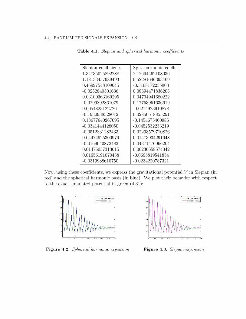
4.4. BANDLIMITED SIGNALS EXPANSION 68
Table 4.1: Slepian and spherical harmonic coefficients
Slepian coefficients Sph. harmonic coeffs.1.34735025892288 2.126944621080361.18133457989493 0.522816463934690.45997548109045 -0.3108172255903-0.0252840301636 0.083944718362050.03100363169295 0.04794941680222-0.0299892861079 0.177539516366190.00548231227261 -0.0274923910878-0.1930938528012 0.028506188552910.18677640267095 -0.1454675460986-0.0341444128050 -0.0452532233219-0.0512831282433 0.022935797108260.04474925300979 0.01473934291648-0.0169040872483 0.043714760662040.01475037313615 0.002366585743420.01656191070438 -0.0695819541854-0.0319988610750 -0.0234220787321
Now, using these coefficients, we express the gravitational potential V in Slepian (inred) and the spherical harmonic basis (in blue). We plot their behavior with respectto the exact simulated potential in green (4.31):
Figure 4.2: Spherical harmonic expansion Figure 4.3: Slepian expansion
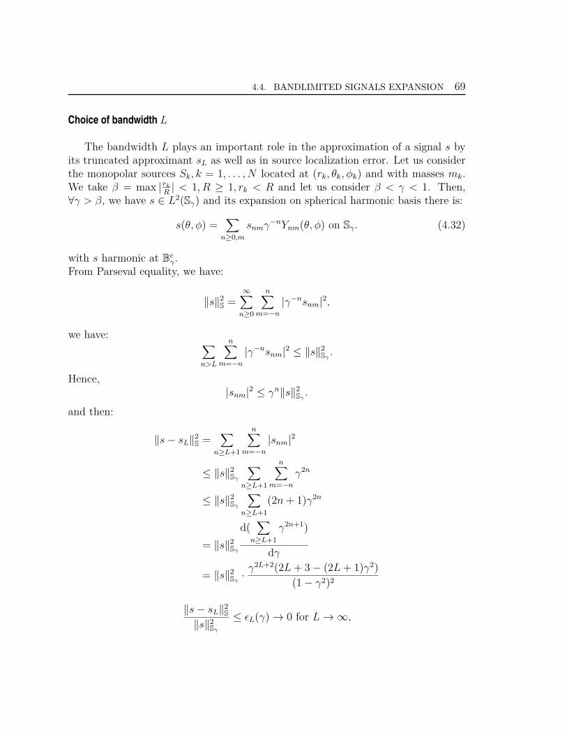
4.4. BANDLIMITED SIGNALS EXPANSION 69
Choice of bandwidth L
The bandwidth L plays an important role in the approximation of a signal s byits truncated approximant sL as well as in source localization error. Let us considerthe monopolar sources Sk, k = 1, . . . , N located at (rk, θk, φk) and with masses mk.We take β = max | rk
R| < 1, R ≥ 1, rk < R and let us consider β < γ < 1. Then,
∀γ > β, we have s ∈ L2(Sγ) and its expansion on spherical harmonic basis there is:
s(θ, φ) =∑
n≥0,m
snmγ−nYnm(θ, φ) on Sγ. (4.32)
with s harmonic at Beγ.
From Parseval equality, we have:
‖s‖2S
=∞∑
n≥0
n∑
m=−n
|γ−nsnm|2,
we have:∑
n>L
n∑
m=−n
|γ−nsnm|2 ≤ ‖s‖2Sγ.
Hence,|snm|2 ≤ γn‖s‖2
Sγ.
and then:
‖s− sL‖2S
=∑
n≥L+1
n∑
m=−n
|snm|2
≤ ‖s‖2Sγ
∑
n≥L+1
n∑
m=−n
γ2n
≤ ‖s‖2Sγ
∑
n≥L+1
(2n+ 1)γ2n
= ‖s‖2Sγ
d(∑
n≥L+1
γ2n+1)
dγ
= ‖s‖2Sγ
· γ2L+2(2L+ 3 − (2L+ 1)γ2)
(1 − γ2)2
‖s− sL‖2S
‖s‖2Sγ
≤ ǫL(γ) → 0 for L → ∞,
4.4. BANDLIMITED SIGNALS EXPANSION 70
where
ǫL(γ) =γ2L+2(2L+ 3 − (2L+ 1)γ2)
(1 − γ2)2
=γ2
(1 − γ2)2Lγ2L(2 +
3L
− (2 +1L
)γ2)
≃ 2γ2
1 − γ2Lγ2L → 0, L → ∞, |γ| < 1
withLγ2L = Le−2L(ln( 1
γ)).
We have used:Le−αL → 0 for L → ∞, α > 0.
Chapter5Singularities of the potential in the ball
The aim of this chapter is the resolution of the density recovery (DR) problemand singularity recovery (SR) problem when the disposed data is the gravitationalpotential and the electrical potential, respectively (monopolar and dipolar sources,respectively). The unified mathematical formulation of these two potential problemsis expressed by [6, 22]:
∆Pot = ρ in B, (5.1)
where Pot can be the gravitational or the electrical potential and the density ρ canbe approximated by a discrete combination of monopolar and dipolar density givenas follows:
f =N∑
k=1
mkδSk+
N∑
k=1
pk.∇δCk, (5.2)
f ≃ ρ, where Sk are monopolar sources, Ck are the dipolar sources, mk the massesof Sk and pk the moments of Ck. For pk = 0 the problem becomes a monopolargeodesy inverse problem and for mk = 0 we have a dipolar EEG inverse problem.We recall the (DR) and (SR) problems for geodesy and EEG:
(DR): Being given boundary data PotS associated to a solution Pot of (5.1)on S (i.e. Pot|S = PotS), find a related density ρ in B (uniqueness properties will bediscussed).
(SR): Being given on S measurements PotS, find a pointwise discrete distri-bution ρN of (a given number) N pointwise monopolar or dipolar sources locatedinside B, such that the associated potential PotN best approximates Pot in quadraticnorm on S.
71
5.1. DENSITY MODELS 72
In [22] an important identifiability result associated with the problem (5.1) and(5.2) is given. The identifiability result permits us to know if the inverse problem iswell posed in the following sense: if two measured potentials Pot1 and Pot2 coincideon Γ∗ (a convenient subset of the sphere S), then they are generated by the samesources. In other words, identifiability means the uniqueness of the inverse problem,see Theorem 5.2.1. Related to the geodesy and EEG inverse problems, well-posednessproperties discussions intervene naturally. This chapter is organized as follows. InSection 5.1, we give the mathematical formulation for some direct and inverse geodesyand EEG problems, then in Section 5.2 some well-posedness results are introduced.We end by Section 5.3 where the best quadratic approximation method is presentedas algorithm for the resolution of both (DR) inverse problems, see [8, 17].
5.1 Density models
The mathematical formulation for the direct and the inverse problems related tothe geodesy and M/EEG that we consider in this thesis is given by the equations:
−∆V = ρ in B , ∆V = 0 in Be = R
3 \ B, (5.3)
where V ∈ L2(R3) and ρ ∈ L2(B) are the gravitational potential and the gravitationaldensity, respectively. In this section, we study the inverse density recovery problems.In fact, the density recovery problem (DR) consists of approximately computing thedensity ρ ∈ L2(B) inside the ball by solving the (SR) problem. For the solutionof this later, we apply the rational approximation techniques given in [8, 17]. Moreprecisely, given V|S on S, we build the "discrete" problem (SR) as an intermediary stepfor the (DR) resolution problem [6, 10]. At this level, we will describe the algorithmthat allows us to go from the data on the sphere to the singularities in the ball B.Hence, the recovery of the discrete density is accomplished. In fact, we are interestedin a density of the following form (relation (5.2) with pk = 0):
ρN =N∑
k=1
mkδSk, (5.4)
which leads to the associated approximated potential VN such that ρN approximatesρ and it is solution of:
−∆VN = ρN in B, ∆VN = 0 in Be and VN best approximates V on L2(S) norm.
(5.5)
5.1. DENSITY MODELS 73
The discrete density ρN can be approximated by a density ρχ which characterizeinclusions zones of the Earth with high concentration. Recall that, when it comesto applications, the surface S of B could be either the Earth boundary, or the scalpof the head. We assume here that the given data VS on S is given via its harmonicspherical expansion coefficients. In this thesis, we use the available data on S or partof S and we apply our proposed Gaussian quadrature method on the sphere to getaccurate approximations of these coefficients.
Density recovery problem
Related to the inverse problem is the direct (forward) problem, which consists infinding the values on S of the potential V solution to (5.3), from the internal densityρ in B. The relation between the density ρ on B and V on S is expressed by theforward operator T :
(Tρ)(y) =∫
B
ρ(x)|x− y|dx for y ∈ S, (5.6)
so that Tρ = V|S for V solution to (5.3) or Te (for data taken on SR, R > 1):
(Teρ)(y) =∫
B
ρ(x)|x− y|dx for y ∈ B
e, (5.7)
whence (Teρ)|S = Tρ. From this, it is easy to see that minimizing the potential inL2(S) comes to minimize ‖ρ‖S. This last problem was studied in [12, 39]. Under aharmonicity constraint, a unique minimizer of ρ is given.
In [16, 51], the authors have given local and global methods for the densityapproximation in the Earth. In [39] and [38] under a constraint of harmonicity akernel or a scaling function is proposed for the density approximation.
In the following, we give a proposition for the existence of the direct problem,and continuity properties of the forward operator T :
Proposition 5.1.1. [39, Thm 2.1] Whenever ρ ∈ L2(B), then V is a solution to(5.3) if and only if V = Teρ, see (5.7).
Remark 5.1.1. The previous Proposition is also valid for pointwise densities ρN
given by (5.4), see [39]. Moreover, it remains true for ρ ∈ L1(B) with supp ρ ⊂ Br ⊂B the ball centered at 0 and of radius r < 1.
Note that in [39], it has been shown that the operator T maps L2(B) → L2(S)continuously and
‖Tρ‖L2(S) ≤ 4π‖ρ‖L2(B).
Another important property of the operator Te is given by the following proposition:
5.1. DENSITY MODELS 74
Proposition 5.1.2. Whenever ρ ∈ L2(B) with supp ρ ⊂ Br, r < 1, then Teρ is acontinuous function on B
e.
Proof. Put Teρ = V . Let y1, y2 ∈ Be:
|V (y2) − V (y1)| = |∫
Br
ρ(x)|x− y2|
dx−∫
Br
ρ(x)|x− y1|
dx|
= |∫
Br
ρ(x)
[1
|x− y2|− 1
|x− y1|
]dx| = |
∫
Br
ρ(x)
[|x− y1| − |x− y2|
|x− y1||x− y2|
]dx|
≤∫
Br
|ρ(x)|[
|y1 − y2||x− y1||x− y2|
]dx,
because ρ ∈ L2(Br) and |x− y| ≥ 1 − r for y ∈ Be.
So,|V (y2) − V (y1)| ≤ c ‖ρ‖L2(B) |y1 − y2|,
with c = cr = (1 − r)2.Hence, |V (y2) − V (y1)| −→ 0 for |y1 − y2| −→ 0.
Remark 5.1.2. The previous Proposition remains true for ρ ∈ L1(B) and supp ρ ⊂Br, r < 1 and for pointwise densities ρN given by (5.4).
In the following, we give other properties of the density ρ and the operator T :The density ρ ∈ L2(B) can be decomposed into a harmonic and an anti-harmonicpart ρ = ρharm + ρanharm such that [39]:
‖ρ‖2B
= ‖ρharm‖2B
+ ‖ρanharm‖2B.
To show this relation we use the next proposition:
Proposition 5.1.3. [39] L2(B) is written as the following direct sum:
L2(B) = Harm(B) ⊕ Anharm(B), (5.8)
whereHarm(B) = H ∈ C2(B)| ∆H = 0 in B,
Anharm(B) = F ∈ L2(B)| 〈F,H〉B = 0,∀H ∈ Harm(B).Proposition 5.1.4. An equivalent decomposition is also given as follows:
L2(B) = Harm(B) ⊕ ∆W 2,20 (B). (5.9)
The space of "anharmonic functions" coincides with those density functions ρ whichhave vanishing associated potential Vρ in B
e:
Anharm(B) = ρ ∈ L2(B) |Teρ = 0.
5.1. DENSITY MODELS 75
Proof. First, we show that Anharm(B) ⊂ ρ ∈ L2(B) |Teρ = 0.The equality Teρ(y) = 0 means:
∫
B
ρ(x)|y − x|dx = (ρ ∗ E3)(y) =
∫
B
ρ(x)E3(y − x)dx = 〈ρ,E3(y − x)〉B = 0,
where E3(y − x) is the fundamental solution of Laplace equation.Let g ∈ ∆W 2,2
0 (B), so g = ∆v, v ∈ W 2,20 (B). Using the second Green’s formula,
we have:
〈g, E3(y − x)〉B =∫
S
∂v(x)∂n
E3(y − x)dx−∫
S
v(x)∂E3(y − x)
∂ndx = 0,
because ∆xE3(y − x) = 0 in B if y ∈ Be and v ∈ W 2,2
0 . Hence, Anharm(B) ⊂ ρ ∈L2(B) |Teρ = 0.
Secondly, we show that Anharm(B) ⊃ ρ ∈ L2(B) |Teρ = 0.Let ρ ∈ L2(B) such as Teρ = 0. This is equivalent to say that 〈ρ,E3(y− x)〉B = 0 fory ∈ B
e. Because E3(y − x) is harmonic for y ∈ Be, we have ρ ∈ Anharm(B).
This proposition is equivalent to say that only the harmonic part of the densitygenerates a non nul exterior potential.
Remark 5.1.3. KerTe = KerT = Anharm(B) = ρ ∈ L2(B) |Teρ = 0 with thetopological supplement Harm(B) in L2(B).
Source recovery problem
(SR) problem has been considered for example in [1] and consists in findinga discrete density in B denoted by ρN , such that TρN = VN |S is close to a givenfunction VS on S, in a sense to be made precise. Note that whenever VS = V|S
for some solution V = Tρ to (5.3), then (SR) leads to a discretization VN of thepotential V (and to the related discrete density ρN , approximating ρ).Given VS on S, we thus introduce the functional FN defined on B
N × RN which
depends on two families of parameters (vectors) (S,m) representing the positionsand masses associated with N monopolar sources, that is:
FN(S,m) = ‖VS − VN‖2S, (5.10)
5.1. DENSITY MODELS 76
where VN = V (N,S,m), S = (Sk) ∈ BN , 0 < r1 ≤ |Sk| ≤ r2 < 1, m = (mk) ∈ R
N ,M ≥ mk ≥ m > 0, for k = 1, . . . , N , where M is the mass of the Earth and
VN(y) =N∑
k=1
mk
|y − Sk| ,∀ y 6= Sk. (5.11)
Then, with ρN =∑N
k=1 mkδSk, we have that VN is a solution to (5.3) associated to
ρN , with VN = TρN .
Remark 5.1.4. Though the Earth density possesses localized zones of high concen-tration, they can though be approximated by pointwise masses or by inclusions [10].
In geophysics literature, the inverse geodesy problem (DR) was intensively stud-ied, see for example [1, 38, 39, 51].
Next, the inverse problem of density recovery related to EEG that we consider inthis thesis is modeled by the equations (2.50). We note in this case that the surfaceS of B is the scalp of the head and after a preliminary cortical mapping step ofdata transmission, we end up with a "filtered" part of the electrical potential whichsatisfies ∆U = 0 in B
e.In the same way as for the monopolar case, we can formulate the direct and theinverse (DR) EEG problem.
The direct problem associated to (SR) is: being given the densityρN =
∑Nk=1 pk.∇δCk
inside the ball B, find the exterior generated potential Uat S.
The density recovery problem (SR) is: being given boundary data US associatedto a solution U of (2.50) on S (i.e. U|S = US), find the related density ρN in B.
Links between (DR) and (SR) problem
To have an approximation of the (DR) problem, we solve the source recovery prob-lem (SR) supposing the discrete density given by a monopolar or dipolar sources dis-tribution. In the geodesy case, because of the non uniformed repartition of the density(different levels of concentration on the Earth), this can be modeled by agglomera-tions of monopolar/dipolar sources contained in small inclusions parametrized by asmall radius ǫ, see Section 5.4.
5.2. EXISTENCE, UNIQUENESS AND STABILITY RESULTS 77
5.2 Existence, uniqueness and stability results
We recall the (SR) inverse geodesy problem with ρN given by (5.4), supposing thatM ≥ mk ≥ m > 0, and the sources considered inside the spherical shell B = B(r1, r2):0 < r1 ≤ |Sk| ≤ r2 < 1. Before solving this problem, we give some existence,uniqueness and stability results. The point-masses determination problem (5.10)was introduced in [1]. In order to study the well-posedeness of the problem, weintroduce details on the existence property.
Problem (SR): For a fixed N
find VN (alternatively, (S,m)) that minimizes (5.10). (5.10′
)
In the following we give a proof of the existence of this problem:
Proposition 5.2.1. For any set of measurements of V , there exists a density ρsuch that Tρ = V ∈ L2(S).
Proof. The existence of solutions VN to problem (5.10′
) is ensured by continuityproperties. The expansion of V , measured at the surface of the unit sphere, in termsof the spherical harmonic basis is given by:
V (1, θ, φ) =∞∑
n=0
n∑
m=−n
cnmYnm(θ, φ), (5.12)
The potential generated by N sources is the sum of the potentials generated by theconsidered point masses.
VN(1, θ, φ) =N∑
k=1
mk
∞∑
n=0
n∑
m=−n
rnk
4π2n+ 1
Ynm(θk, φk)Ynm(θ, φ), (5.13)
with cnm the coefficients of the development of V in spherical harmonic basis. Forgetting the spherical harmonic expansion of the discrete gravitational potential (5.11)we denote by lk the Euclidean distance between X and Sk with
lk =√
1 − 2rk cosψk + r2k, (5.14)
where ψk is the spherical distance between X and Sk. Then, we have:
1lk
=1
√1 − 2rk cosψk + r2
k
=1rk
∞∑
n=0
rn+1k Pn(cosψk). (5.15)
5.2. EXISTENCE, UNIQUENESS AND STABILITY RESULTS 78
Using the addition formula for spherical harmonics (2.38), we get:
1lk
=∞∑
n=0
rnk
4π2n+ 1
Ynm(θk, φk)Ynm(θ, φ). (5.16)
Then, we obtain (5.13). Using the development of V and VN on the spherical har-monic basis, the functional FN(S,m) = ‖VS − VN‖2
Sbecomes:
minS∈BN ,m∈RN
‖b− A(S)m‖2S, (5.17)
where, the entries of b and A(S) are given by:
bI(n,m) = cnm
( 1R
)n, I(n,m) = 1, 2, . . . ,
AI(n,m)k(S) =4π
(2n+ 1)rn
kYnm(θk, φk), I(n,m) = 1, 2 . . . , k = 1, . . . , N,
with I(n,m) =∑n
l=0(2l+ 1) − n+m = n2 + n−m+ 1, −n ≤ m ≤ n. We note that
the functional FN is continuous on the ball BN × [0,M ]N , 0 ≤N∑
k=1
mk ≤ M .
The problem (5.5) is ill posed. A condition on this problem such that the solutionexists is the next compatibility condition:
∫
S
gdω = −N∑
k=1
mk,
with g = ∂V∂n
. Then, the solution is unique up to an additive constant.For the (SR) problem, the uniqueness (i.e. identifiability) of the solution of (5.10)
is establish in [22], see the next theorem for pk = 0 in (5.2):
Theorem 5.2.1. [22] Let Vi, i = 1, 2 be the solution of the problems
∆Vi = F i in B∂Vi
∂n= g on S
V = f on S
(5.18)
such that V1 = V2 on Γ∗ which is a subset with non-void interior of S. Then V1 = V2,i.e.
S(1)k = S
(2)k ,m
(1)k = m
(2)k , k = 1, . . . , N.
where Sk are monopolar sources and mk their masses.
5.3. RESOLUTION SCHEMES 79
A general stability result is given by Theorem 2.2.1. Next, we give some existenceand stability results associated with the EEG problem. The identifiability Theorem5.2.1 remains valid for mk = 0 and pk 6= 0. The direct problem (2.50) is well-posedon the Hilbert quotient space W 1,2(B)/R under the compatibility condition [22]:
∫
Γgdω =
∫
Γ
∂U
∂ndω = 〈ρN , 1〉B (5.19)
where W 1,2 is the Sobolev space, U the electrical potential. Note that if f1, f2 ∈W 1,2(B) with f1 = f2 + constant, then f1 = f2 in W 1,2(B)/R.
Another result is given in [6].
Proposition 5.2.2. Given a dipolar source distribution Ck, k = 1, . . . , N of momentspk, the potential U generated by this distribution verifies (2.50), where the current
flux belongs to W− 12
,2(Γ) with ∫
S
gdω = 0.
Then, the direct EEG problem (2.50) admits a unique solution up to an additive
constant and the solution U belongs to W12
,2(S).
The identifiability Theorem 5.2.1 can be seen as a uniqueness result [22, 55]: iftwo measured potentials U1 and U2 coincide on Γ∗, a non void-interior subset of S,then they are generated by the same sources.
Stability: If two potentials generated by two distributions of N dipolar sourceshave close values on the boundary S, then the corresponded distributions are alsoclose rapported to a distance [22, 53]. A local stability for EEG problem is given in[21]:
Theorem 5.2.2. If ϕh = (pk, Ck)1≤k≤N ∈ (R3 ×B)N such that ϕh → ϕ if h → 0 andif we denote by fh the data on Γ∗ corresponding to ϕh, then:
limh→0
‖f − fh‖Γ∗
|h| > 0.
5.3 Resolution schemes
A short description of some resolution methods was introduced in Chapter 1. Inthis thesis, the (SR) problem is solved by using the best quadratic approximation on2D combined with our scheme for the extrapolation of the potential to whole spherevia Slepian functions basis and the computation of spherical harmonic expansioncoefficients of this later.
5.3. RESOLUTION SCHEMES 80
Our resolution procedure
Once the data is estimated over the whole sphere S (geodesy, M/EEG) by solving(TP), the next step in the resolution of the inverse problem (IP), is the sourcerecovery problem (SR). The resolution of (SR) problem in the ball B involves 3steps:
• Planar sectionsThe ball B is sliced along a family of parallel sections, perpendicular to a chosenaxis. The intersection between B and the planar sections gives us a family ofdisks where we apply the best quadratic rational approximation.
• Best quadratic rational approximation on circlesThe 2D approximation techniques are used to find the planar singularities onthe disks obtained in the previous step.
• 3D sources localizationThe sources are localized in 3D by analyzing the planar singularities inducedby sources or masses which are superposed.
Remark 5.3.1. In order to get more accuracy on the localization process and to sep-arate the sources, the detection step must be performed with several slicing directions.
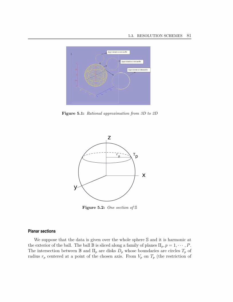
5.3. RESOLUTION SCHEMES 81
Figure 5.1: Rational approximation from 3D to 2D
xy
z
r p Tp
Figure 5.2: One section of S
Planar sections
We suppose that the data is given over the whole sphere S and it is harmonic atthe exterior of the ball. The ball B is sliced along a family of planes Πp, p = 1, · · · , P .The intersection between B and Πp are disks Dp whose boundaries are circles Tp ofradius rp centered at a point of the chosen axis. From Vp on Tp (the restriction of
5.3. RESOLUTION SCHEMES 82
the potential V on the circles Tp, i.e. V \Tp), we build the complex rational variablefunction fp on the unit circle Tp. Due to the N sources Ck, fp has N singularities z−
k,p
(related to the positions of Ck) inside the disk Dp (as well as N related singularitiesz+
k,p outside the closed disk Dp). The data fp is assumed to be given either by anumber of its pointwise values on Tp or by a number of its Fourier coefficients, usingthe spherical harmonics expansions of VS .
Remark 5.3.2. For building the function fp on the circles, we use the relation
z = r2p
z, with z the affix of the points where we take the measurements, see [8].
Remark 5.3.3. In [8, 17], the data is available over whole the sphere S and thecoefficients of the spherical harmonic expansion of the data are computed by solvinga linear system of equations that might be unstable. Our proposed method works withdata potential known only in a region of the sphere, like belt or spherical caps. Also,the coefficients are computed by using the Gauss-Legendre quadrature.
Once we can localize the singularities z−k,p, this leads to an estimate of Ck. The
relation between the singularities z−k,p and the sources Ck is given by the next propo-
sition [56]:
Proposition 5.3.1. We suppose zk 6= 0, k ∈ 1, . . . n. Then:
arg(z−k,p) = arg(zk) and max
p=1...P|z−
k,p| = zk
This allows us to determine the number N of sources.
The function fp has the following properties:
1. If there exists just one source (N = 1), then fp is a rational function with apole (single or triple) in Dp at z1,p.
2. If there are more than one source (N ≥ 2), fp is not anymore a rationalfunction. In this case, fp can still be approximated on the boundary Tp by arational function with poles in Dp [8, 9].
Best quadratic rational approximation on circles
At the origin, the rational approximation was mainly used in systems theory,control theory and signal treatment [11]. The software used for the inverse sourceproblem identification (Matlab software RARL2, see [37]) was first implementedfor the resolution of frequencies filters identification problems in signal [21]. Theseproblems consist in approximating the transfer function of a system by a rational
5.3. RESOLUTION SCHEMES 83
function with poles in D, given pointwise values of the transfer function on the unitcircle T of C. Before describing the algorithm we need to introduce Rm to be theset of rational functions Rm with less than m poles in the unit disk D:
Rm =pm
qm
, where pm, qm are polynomials such that deg pm < deg qm ≤ m, roots of qmbelong to D
A best quadratic rational approximant to fp in Rm is a function R∗m ∈ Rm which
verify:‖fp −R∗
m‖T = minRm∈Rm
‖fp −Rm‖T (5.20)
for the L2(T) norm. As we see in the previous step, the function fp is computedon each circle Tp. To apply the best quadratic rational approximant of fp we needto get the norm L2 on the unit circle T. For this, a normalization step of fp isrequired. Existence and uniqueness in problem (5.20) are studied in [26]. For eachsection p, we compute the best meromorphic approximant of the function fp and thesingularities zk,p are approximated by the poles of the best approximant of fp. Thisstep is repeated for each section and the poles are gathered in groups which give usan estimation of the number N of sources and of their positions Ck.
Remark 5.3.4. If the function fp to be approximated is a rational function of degreem′, the best approximant of fp of degree m coincides with fp for m ≥ m′.
3D source localization
This step "from 2D to 3D" consists in superposing all the estimated singularitiesand estimating the positions of sources. To each k fixed and each axis section, isassociated a singularity line which connects together the singularities zk,p of fp whenp varies for k fixed. When the sources are "well separated", the convergence of thepoles of the best approximant is better for the sections close to the sources. Closerwe are to the section where the source is located, better the poles of the rationalapproximant gather towards the induced singularity. From this remark, in order toget more accuracy on the localization process, it is indicated to take several slicingdirections. Each line lk is associated with one of the sources Ck and has the followingtheoretical properties [17]:
• lk lies in a half-plane containing Ck and orthogonal to the slicing plane Π.
• lk goes through its associated source Ck. If we look to the ball B from thetop of the slicing axis, the source Ck is found at the maximum modulus ofsingularities.
5.4. OTHERS DENSITY MODELS 84
The singularity lines lk associated to various slicing directions Π intersect at thesources which allows to better estimate their positions.
Remark 5.3.5. For both cases i.e. monopolar (geodesy inverse problem) and dipolardensity (EEG inverse problem, see [17]), the same approximation scheme can be usedin order to solve the discretization issue (SR) of the initial (DR) problem. In otherwords, using the best quadratic rational approximantion we solve the (SR) problemfor geodesy and EEG and the solution of this problem gives us an approximant of the(DR) problem.
5.4 Others density models
Due to different levels of concentration of the Earth density, it can be approximatedby different models. As we already saw, one of the appropriate model is that one ofthe monopolar masses. In the following, we describe briefly a case when the (Earth)potential V is generated by a density denoted by cωχω which is concentrated insidea ball ω of radius ǫ and centered in y0 contained in the unit ball B which modelthe Earth [10, 25]. This new model of density allows us to compute an approximantfor (DR) problem. In the complementary part of the ball, B \ ω, the correspondeddensity has the constant value cT .We have the equation :
∆V =
0, R3 \ B
cT , in B \ ωcω, in ω
= ρχ,
with cω, cT ∈ R+, cω >> cT .
∆V = cTχB\ω + cωχω = cTχB + (cω − cT )χω = ρχ.
For subsets A ⊂ Rn, χA is the indicator function with:
χA(x) =
1 if x ∈ A;0 if x /∈ A.
Proposition 5.4.1. The potential generated by the above density ρ ∈ L2(B) coin-cides, up to an additive constant, with a potential issued from a pointwise mass aty0.
5.4. OTHERS DENSITY MODELS 85
Proof. We have:
V (x) =∫
B
cT + χω(y)(cω − cT )dy|x− y| ,
V (x) = cT
∫
B
dy|x− y| + (cω − cT )
∫
ω
dy|x− y| . (5.21)
Now, if we take
U(y) = Ux(y) =1
|x− y| = E3(x− y) with ∆yUx = 0 in B.
applying the Theorem 2.2.3 of mean-value property, we have:
143π
∫
B
dy|x− y| = Ux(y = 0) =
1|x| = 1, |x| = 1 (unit ball). (5.22)
Consequently, we have: ∫
B
dy|x− y| =
4π3.
For the ball denoted by ω = ω(y0, ǫ), we obtain:
143πǫ3
∫
ω
dy|x− y| = Ux(y = y0) =
1|x− y0|
= E3(x− y0), (5.23)
∫
ω
dy|x− y| =
ǫ34π3|x− y0|
=ǫ34π
3E3(x− y0).
From (5.21), (5.22) and (5.23) we obtain:
V (x) =4π3
[cT + ǫ3(cω − cT )E3(x− y0)
]. (5.24)
In the case when the density of the Earth is model by 6 dipoles (or a finite number ofpoint masses) placed inside a small ball ω(x0, ǫ), the associated potential is the sumof the individual contributions. For solving the inverse problem we use the rationalapproximation technique described in Section 5.3. The unit ball B is intersected by5 parallel planes orthogonal to the z-th axis, so that we obtain a family of 2D disksDp, p = −5, . . . , 5. The next image represents the approximation result on the 5-thsection: the blue points are the poles of the approximant and those in red the truesingularities of sources. The next two images represent a 3D visualization of thesphere after we apply the best meromorphic approximant on each circle. On the firstfigure we can see the poles of each 2D-approximant (in blue) for the 6 sources (ingreen). In the second case, the figure is seen from above.
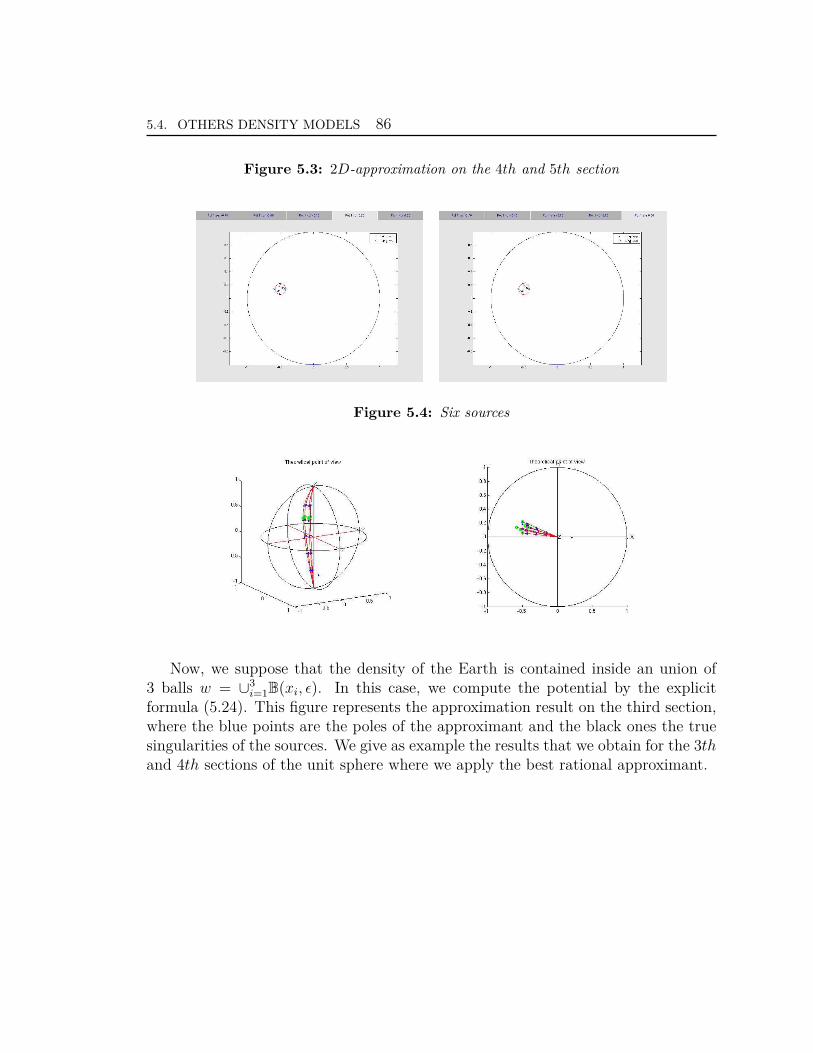
5.4. OTHERS DENSITY MODELS 86
Figure 5.3: 2D-approximation on the 4th and 5th section
Figure 5.4: Six sources
Now, we suppose that the density of the Earth is contained inside an union of3 balls w = ∪3
i=1B(xi, ǫ). In this case, we compute the potential by the explicitformula (5.24). This figure represents the approximation result on the third section,where the blue points are the poles of the approximant and the black ones the truesingularities of the sources. We give as example the results that we obtain for the 3thand 4th sections of the unit sphere where we apply the best rational approximant.
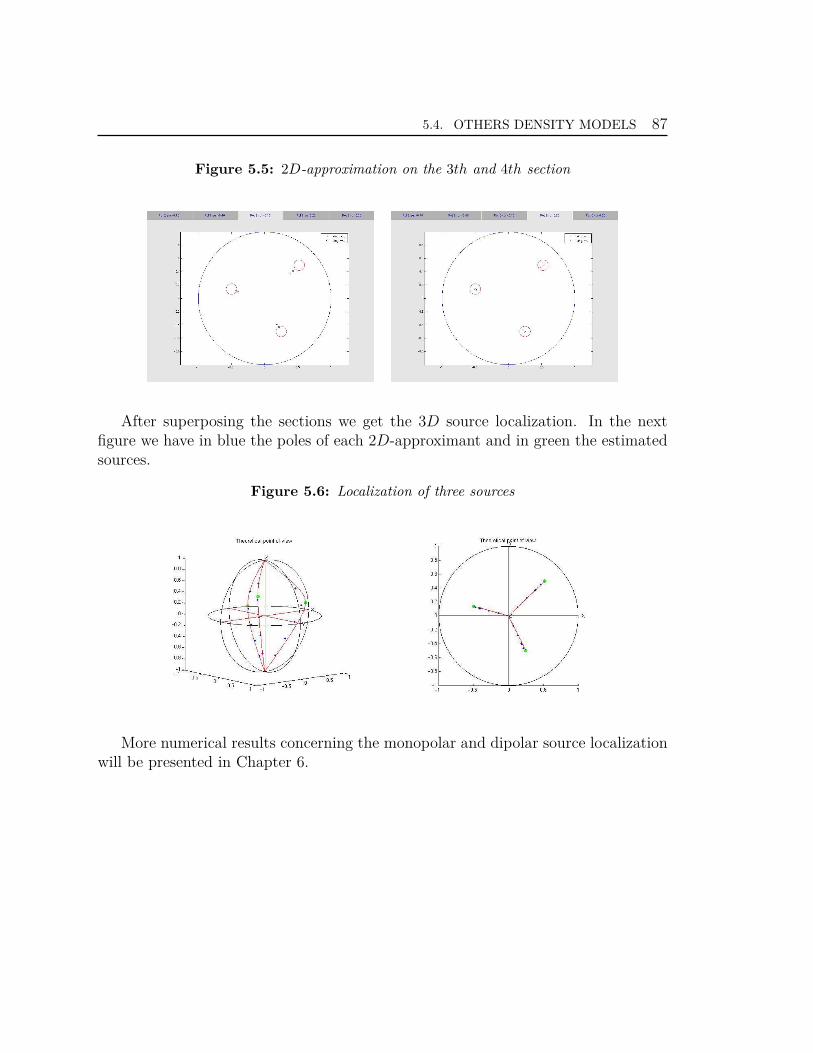
5.4. OTHERS DENSITY MODELS 87
Figure 5.5: 2D-approximation on the 3th and 4th section
After superposing the sections we get the 3D source localization. In the nextfigure we have in blue the poles of each 2D-approximant and in green the estimatedsources.
Figure 5.6: Localization of three sources
More numerical results concerning the monopolar and dipolar source localizationwill be presented in Chapter 6.

5.4. OTHERS DENSITY MODELS 88
Chapter6Numerical results
In this chapter, we give various examples that illustrate the results of this thesis.The scheme used to obtain these numerical results is explained in the following. Wealready saw that the resolution of the inverse problem (IP) involves the resolutionof two problems: the transmission data problem (TP) and density recovery (DR)problem. In practice, as we know, the data is available just on some regions asthe north hemisphere of the head (M/EEG) or above continents, spherical caps,etc. (geodesy). To represent these data, we have build a new adaptive basis. TheChapter 3 provides a new efficient method for building the convenient Slepianbasis. This method is based on Gauss-Legendre quadrature. The step which consistsin passing from the partial data expressed in the new Slepian basis, towards thecomplete data over the whole sphere S and expressed in spherical harmonic basis,is called the transmission data problem (TP). For more details, see Chapter 4.For (DR) resolution problem via the best quadratic rational approximation on 2Don sections, we need the coefficients of the spherical harmonic expansion of thedata over the sphere. In this thesis we have given an accurate method based onGauss-Legendre quadrature, for the computation of the coefficients of the sphericalharmonic development. This passage involves some steps and it was implemented inMAPLE:
• We compute the spherical harmonic expansion of the potential (gravitational orelectrical) truncated up to a bandwidth L. For this, informations as bandwidth,angles of spherical caps (belts) and positions of sources are read from a filecalled input.txt;
• Once we know the potential and the Slepian basis, we compute the coefficientsof its Slepian expansion (as integrals over the region Θ between the potential
89
90
and Slepian basis, see Chapter 4, relation (4.9));
• Knowing the coefficients of the Slepian expansion and Slepian functions, wehave to built the potential by using the Slepian basis;
• We compute the coefficients of the spherical harmonic expansion as integralover the sphere between the potential and the spherical harmonic basis.
The output data furnished by this MATLAB software will give informations whichserve as input for the MATLAB software FindSources3D. This output data willbe exported from MAPLE as a file called output.txt and it contains the truncationbandwidth of the potential, the angles associated with the the region (spherical caps,belts), the spherical harmonic coefficients and the nodes on which the potential datawas evaluated over the whole sphere. For a better organization of files, the name ofoutput.txt will change in function of the variables values.The next step of the (IP) resolution problem is the density recovery (DR) problemsolved by FindSources3D (INRIA, APICS team, see [24]) that uses the best quadraticapproximation on 2D planar sections, see Chapter 5. Chapter 6 is presented suchthat to illustrate numerical tests which was obtained by using the MAPLE andMATLAB codes and which corresponds to (TP) and (DR) problems. Firstly, weintroduce the monopolar case of geodesy masses model and in a second time weconsider the dipolar case for EEG.Choice of the bandwidth LThe truncated spherical harmonics expansion of the potential data represents anapproximation of the real potential. The choice of the bandwidth L affects thereconstruction of the data and the precision of the source localization. We makedifferent choices of the bandwidth L in order to show the fact that greater thebandwidth L is, better we localize the sources. We introduce some symbols:
• the singularities zk,p of fp are represented by green points.
• the sources Ck are marked by red points.
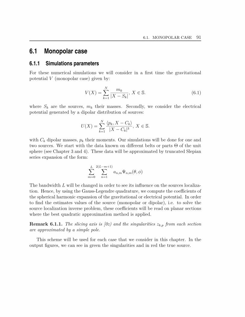
6.1. MONOPOLAR CASE 91
6.1 Monopolar case
6.1.1 Simulations parameters
For these numerical simulations we will consider in a first time the gravitationalpotential V (monopolar case) given by:
V (X) =N∑
k=1
mk
|X − Sk| , X ∈ S. (6.1)
where Sk are the sources, mk their masses. Secondly, we consider the electricalpotential generated by a dipolar distribution of sources:
U(X) =N∑
k=1
〈pk, X − Ck〉|X − Ck|3 , X ∈ S.
with Ck dipolar masses, pk their moments. Our simulations will be done for one andtwo sources. We start with the data known on different belts or parts Θ of the unitsphere (see Chapter 3 and 4). These data will be approximated by truncated Slepianseries expansion of the form:
L∑
m=0
2(L−m+1)∑
n=1
an,mΨn,m(θ, φ)
The bandwidth L will be changed in order to see its influence on the sources localiza-tion. Hence, by using the Gauss-Legendre quadrature, we compute the coefficients ofthe spherical harmonic expansion of the gravitational or electrical potential. In orderto find the estimates values of the source (monopolar or dipolar), i.e. to solve thesource localization inverse problem, these coefficients will be read on planar sectionswhere the best quadratic approximation method is applied.
Remark 6.1.1. The slicing axis is [0z) and the singularities zk,p from each sectionare approximated by a simple pole.
This scheme will be used for each case that we consider in this chapter. In theoutput figures, we can see in green the singularities and in red the true source.
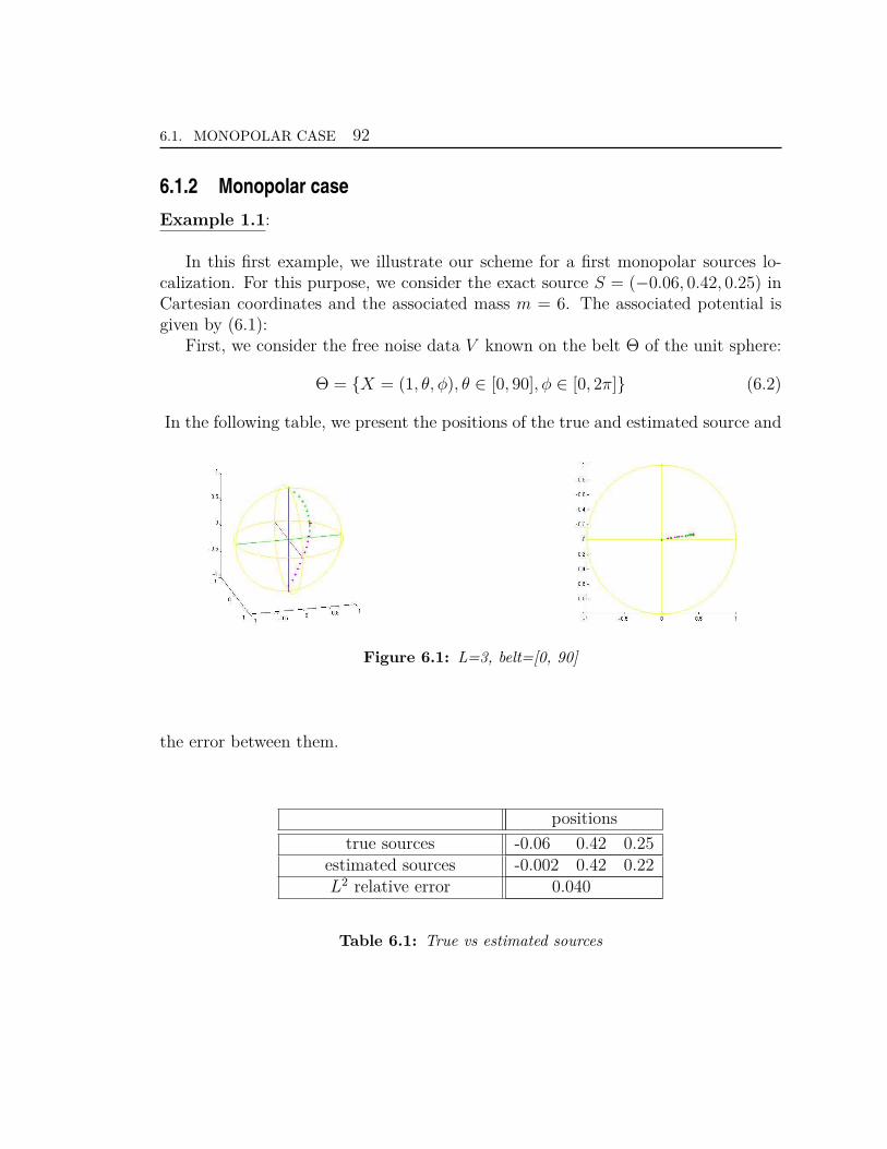
6.1. MONOPOLAR CASE 92
6.1.2 Monopolar case
Example 1.1:
In this first example, we illustrate our scheme for a first monopolar sources lo-calization. For this purpose, we consider the exact source S = (−0.06, 0.42, 0.25) inCartesian coordinates and the associated mass m = 6. The associated potential isgiven by (6.1):
First, we consider the free noise data V known on the belt Θ of the unit sphere:
Θ = X = (1, θ, φ), θ ∈ [0, 90], φ ∈ [0, 2π] (6.2)
In the following table, we present the positions of the true and estimated source and
Figure 6.1: L=3, belt=[0, 90]
the error between them.
positionstrue sources -0.06 0.42 0.25
estimated sources -0.002 0.42 0.22L2 relative error 0.040
Table 6.1: True vs estimated sources
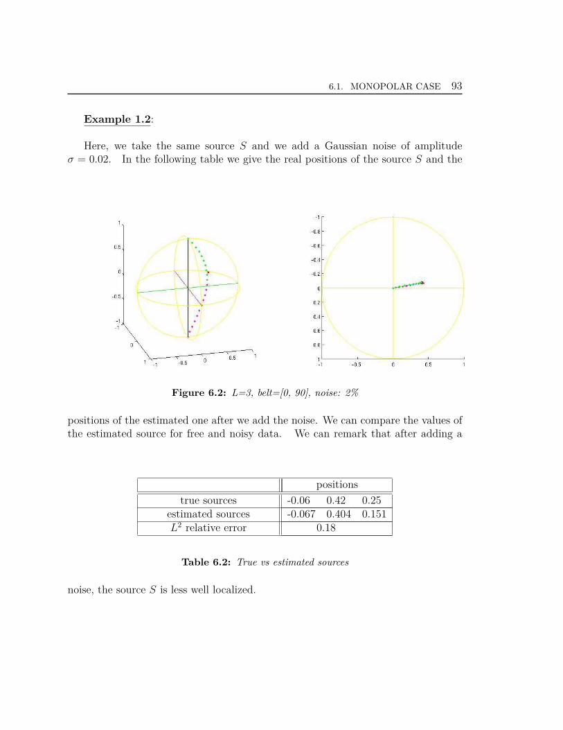
6.1. MONOPOLAR CASE 93
Example 1.2:
Here, we take the same source S and we add a Gaussian noise of amplitudeσ = 0.02. In the following table we give the real positions of the source S and the
Figure 6.2: L=3, belt=[0, 90], noise: 2%
positions of the estimated one after we add the noise. We can compare the values ofthe estimated source for free and noisy data. We can remark that after adding a
positionstrue sources -0.06 0.42 0.25
estimated sources -0.067 0.404 0.151L2 relative error 0.18
Table 6.2: True vs estimated sources
noise, the source S is less well localized.
6.1. MONOPOLAR CASE 94
Example 1.3:
In this example we consider L = 6, θ ∈ [0, 90]. When the data is available overthe north hemisphere θ ∈ [0, 90], we notice that for bigger L, the source is betterlocalized. The data is supposed without noise. Comparing to the numerical test
Figure 6.3: L=6, belt=[0, 90]
positionstrue sources -0.06 0.42 0.25
estimated sources -0.06 0.42 0.23L2 relative error 0.00061
Table 6.3: True vs estimated sources
for L = 3, when we obtained an error localization of order 10−2, for L = 6 we havea better localization with an error of order 10−4.
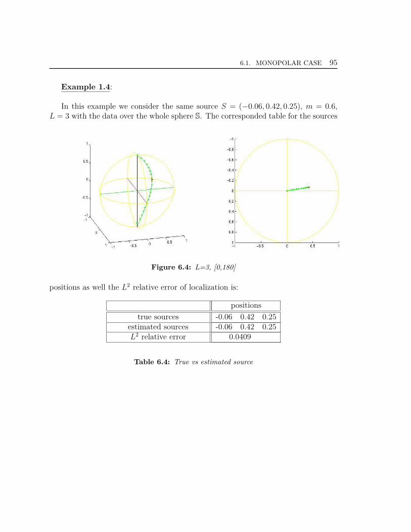
6.1. MONOPOLAR CASE 95
Example 1.4:
In this example we consider the same source S = (−0.06, 0.42, 0.25), m = 0.6,L = 3 with the data over the whole sphere S. The corresponded table for the sources
Figure 6.4: L=3, [0,180]
positions as well the L2 relative error of localization is:
positionstrue sources -0.06 0.42 0.25
estimated sources -0.06 0.42 0.25L2 relative error 0.0409
Table 6.4: True vs estimated source
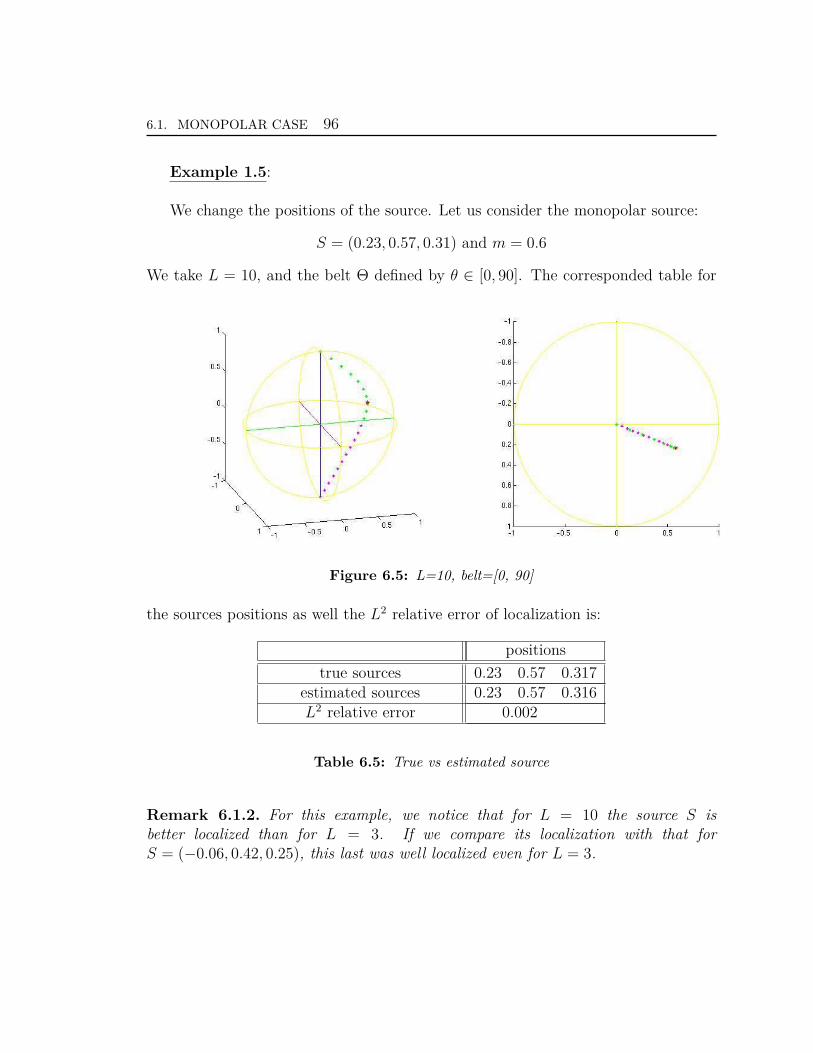
6.1. MONOPOLAR CASE 96
Example 1.5:
We change the positions of the source. Let us consider the monopolar source:
S = (0.23, 0.57, 0.31) and m = 0.6
We take L = 10, and the belt Θ defined by θ ∈ [0, 90]. The corresponded table for
Figure 6.5: L=10, belt=[0, 90]
the sources positions as well the L2 relative error of localization is:
positionstrue sources 0.23 0.57 0.317
estimated sources 0.23 0.57 0.316L2 relative error 0.002
Table 6.5: True vs estimated source
Remark 6.1.2. For this example, we notice that for L = 10 the source S isbetter localized than for L = 3. If we compare its localization with that forS = (−0.06, 0.42, 0.25), this last was well localized even for L = 3.
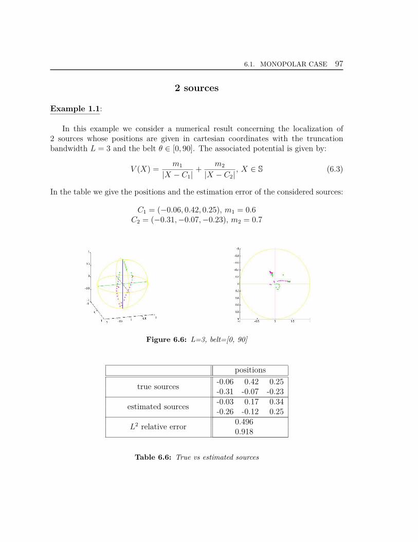
6.1. MONOPOLAR CASE 97
2 sources
Example 1.1:
In this example we consider a numerical result concerning the localization of2 sources whose positions are given in cartesian coordinates with the truncationbandwidth L = 3 and the belt θ ∈ [0, 90]. The associated potential is given by:
V (X) =m1
|X − C1|+
m2
|X − C2|, X ∈ S (6.3)
In the table we give the positions and the estimation error of the considered sources:
C1 = (−0.06, 0.42, 0.25), m1 = 0.6C2 = (−0.31,−0.07,−0.23), m2 = 0.7
Figure 6.6: L=3, belt=[0, 90]
positions
true sources-0.06 0.42 0.25-0.31 -0.07 -0.23
estimated sources-0.03 0.17 0.34-0.26 -0.12 0.25
L2 relative error0.4960.918
Table 6.6: True vs estimated sources
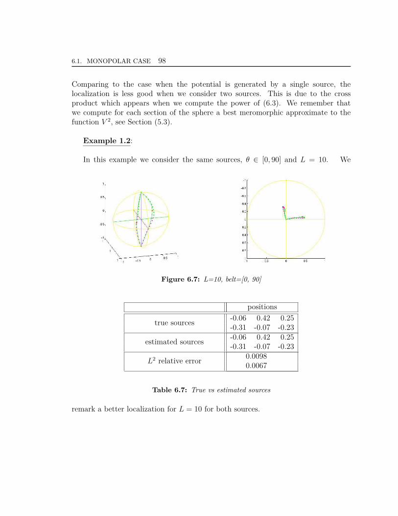
6.1. MONOPOLAR CASE 98
Comparing to the case when the potential is generated by a single source, thelocalization is less good when we consider two sources. This is due to the crossproduct which appears when we compute the power of (6.3). We remember thatwe compute for each section of the sphere a best meromorphic approximate to thefunction V 2, see Section (5.3).
Example 1.2:
In this example we consider the same sources, θ ∈ [0, 90] and L = 10. We
Figure 6.7: L=10, belt=[0, 90]
positions
true sources-0.06 0.42 0.25-0.31 -0.07 -0.23
estimated sources-0.06 0.42 0.25-0.31 -0.07 -0.23
L2 relative error0.00980.0067
Table 6.7: True vs estimated sources
remark a better localization for L = 10 for both sources.
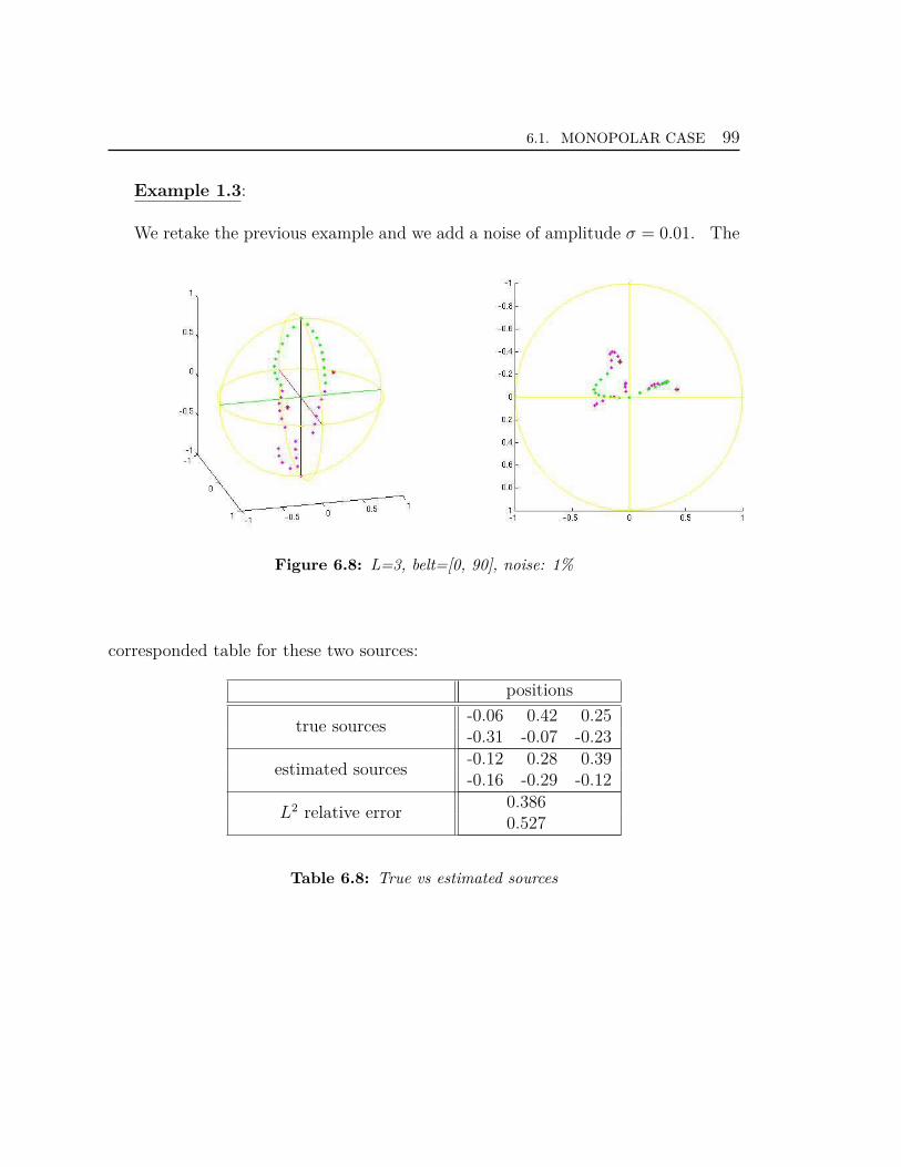
6.1. MONOPOLAR CASE 99
Example 1.3:
We retake the previous example and we add a noise of amplitude σ = 0.01. The
Figure 6.8: L=3, belt=[0, 90], noise: 1%
corresponded table for these two sources:
positions
true sources-0.06 0.42 0.25-0.31 -0.07 -0.23
estimated sources-0.12 0.28 0.39-0.16 -0.29 -0.12
L2 relative error0.3860.527
Table 6.8: True vs estimated sources
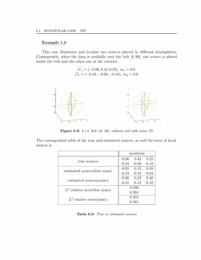
6.1. MONOPOLAR CASE 100
Example 1.4:
This case illustrates and localize two sources placed in different hemispheres.Consequently, when the data is available over the belt [0, 90], one source is placedinside the belt and the other one at the exterior.
C1 = (−0.06, 0.42, 0.25), m1 = 0.6C2 = (−0.34,−0.08,−0.18), m2 = 0.6
Figure 6.9: L=3, belt=[0, 90], without and with noise 2%
The corresponded table of the true and estimated sources, as well the error of local-ization is:
positions
true sources-0.06 0.42 0.25-0.34 -0.08 -0.18
estimated sources(free noise)-0.01 0.13 0.16-0.19 -0.10 -0.04
estimated sources(noise)-0.06 0.23 0.40-0.31 -0.12 -0.10
L2 relative error(free noise)0.5860.384
L2 relative error(noise)0.4530.561
Table 6.9: True vs estimated sources
6.2. DIPOLAR CASE 101
6.2 Dipolar case
1 source
Example 1.1:
In [23], the author has developed a scheme for the source localization. This schemeis based on the use of an initial guess of the exact locations of the sources combinedwith the boundary element method to calculate a cost function J and its gradientassociated with the (SR) problem. Then, an iterative minimization algorithm is usedto compute the approximate location of the sources.
In [23], it was applied the previous scheme for one dipolar source with Ctrue =(0.12, 0.12, 0.12), ptrue = (0.70, 0, 0.70) and taking two different starting points C1
0 =(0.63, 0.1, 0.75), p1
0 = (0.4, 0, 0.2) and C20 = (0.5, 0.3, 0.9), p2
0 = (0.4, 0.3,−0.2). Thefirst value is closer to the exact solution than the second one. The data are consideredto be known on the whole boundary of the sphere, with no added noise.
In the case when the data are considered known just on the belt Θ = [0, 90], weuse the method of Simons [46] to have the data expansion on Slepian basis. After,we use FindSource3D software for source localization and we find the estimatedsource Cestim = (0.118, 0.117, 0.132) with the L2 relative error equal to 0.0579. Wenote that although the scheme introduced in [23] gives a slightly better result (anerror of order 10−5 and 10−4 for the initial guess C1
0 , respectively C20), our method
has the advantage to not require an initial accurate guess of the source localization.Also, we have repeated the previous example with an added Gaussian noise withσ = 0.02 and truncation bandwidth L = 10 and find the location of the sourceCestim = (0.121, 0.117, 0.151) and an error equal to 0.149. The following numericaltests are done by using the method of Simons when we dispose of partial data onthe sphere.
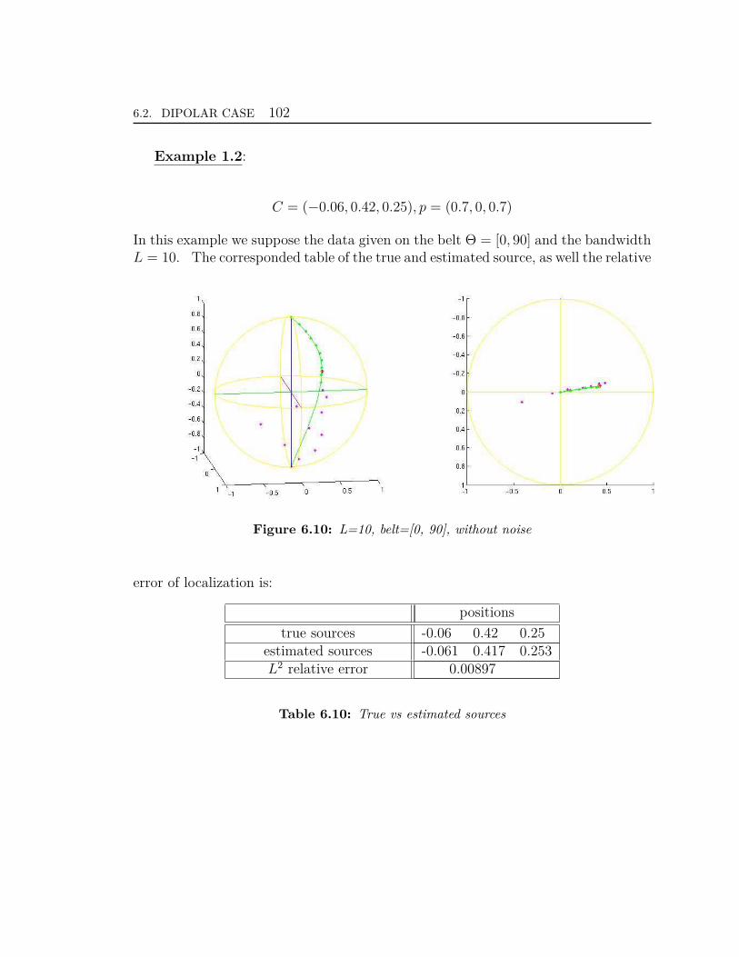
6.2. DIPOLAR CASE 102
Example 1.2:
C = (−0.06, 0.42, 0.25), p = (0.7, 0, 0.7)
In this example we suppose the data given on the belt Θ = [0, 90] and the bandwidthL = 10. The corresponded table of the true and estimated source, as well the relative
Figure 6.10: L=10, belt=[0, 90], without noise
error of localization is:
positionstrue sources -0.06 0.42 0.25
estimated sources -0.061 0.417 0.253L2 relative error 0.00897
Table 6.10: True vs estimated sources
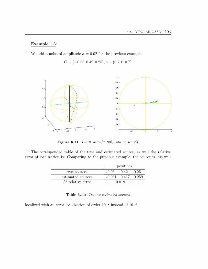
6.2. DIPOLAR CASE 103
Example 1.3:
We add a noise of amplitude σ = 0.02 for the previous example:
C = (−0.06, 0.42, 0.25), p = (0.7, 0, 0.7)
Figure 6.11: L=10, belt=[0, 90], with noise: 2%
The corresponded table of the true and estimated source, as well the relativeerror of localization is: Comparing to the previous example, the source is less well
positionstrue sources -0.06 0.42 0.25
estimated sources -0.061 0.417 0.259L2 relative error 0.019
Table 6.11: True vs estimated sources
localized with an error localization of order 10−2 instead of 10−3.
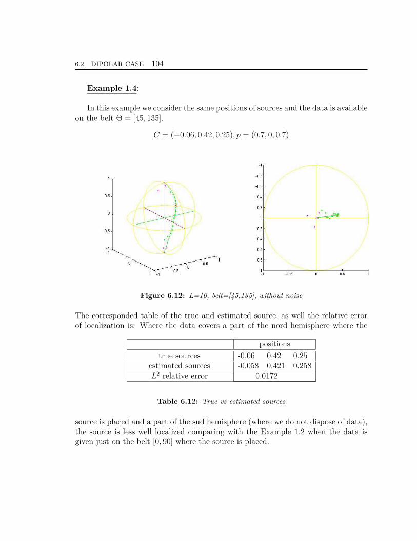
6.2. DIPOLAR CASE 104
Example 1.4:
In this example we consider the same positions of sources and the data is availableon the belt Θ = [45, 135].
C = (−0.06, 0.42, 0.25), p = (0.7, 0, 0.7)
Figure 6.12: L=10, belt=[45,135], without noise
The corresponded table of the true and estimated source, as well the relative errorof localization is: Where the data covers a part of the nord hemisphere where the
positionstrue sources -0.06 0.42 0.25
estimated sources -0.058 0.421 0.258L2 relative error 0.0172
Table 6.12: True vs estimated sources
source is placed and a part of the sud hemisphere (where we do not dispose of data),the source is less well localized comparing with the Example 1.2 when the data isgiven just on the belt [0, 90] where the source is placed.
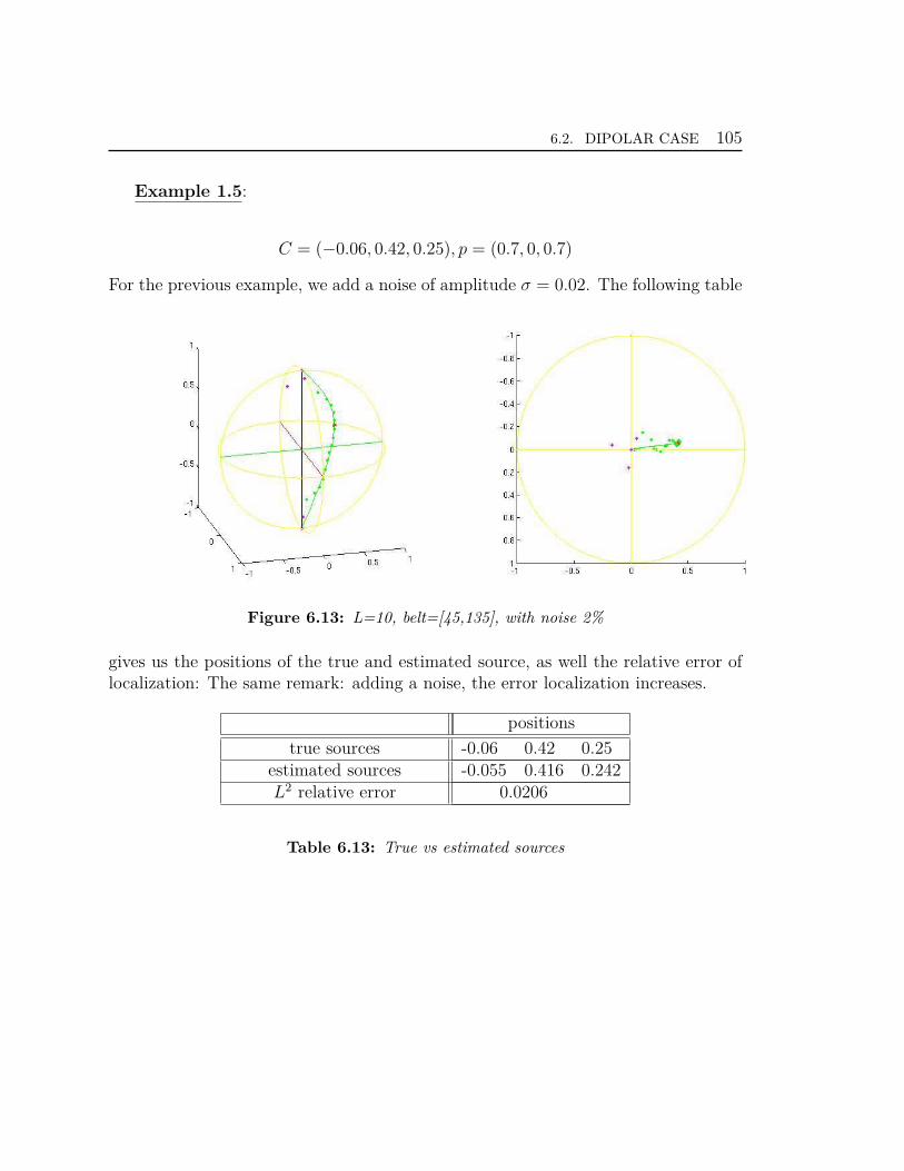
6.2. DIPOLAR CASE 105
Example 1.5:
C = (−0.06, 0.42, 0.25), p = (0.7, 0, 0.7)
For the previous example, we add a noise of amplitude σ = 0.02. The following table
Figure 6.13: L=10, belt=[45,135], with noise 2%
gives us the positions of the true and estimated source, as well the relative error oflocalization: The same remark: adding a noise, the error localization increases.
positionstrue sources -0.06 0.42 0.25
estimated sources -0.055 0.416 0.242L2 relative error 0.0206
Table 6.13: True vs estimated sources
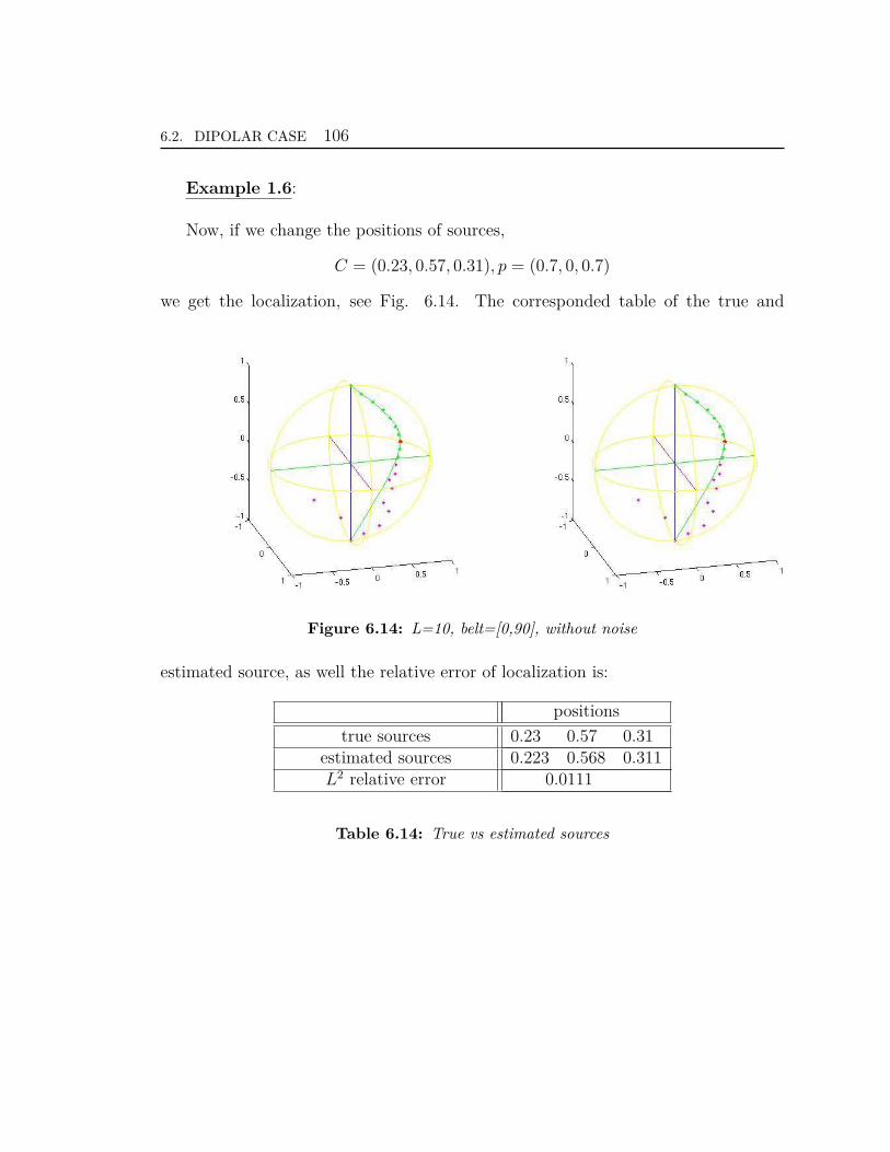
6.2. DIPOLAR CASE 106
Example 1.6:
Now, if we change the positions of sources,
C = (0.23, 0.57, 0.31), p = (0.7, 0, 0.7)
we get the localization, see Fig. 6.14. The corresponded table of the true and
Figure 6.14: L=10, belt=[0,90], without noise
estimated source, as well the relative error of localization is:
positionstrue sources 0.23 0.57 0.31
estimated sources 0.223 0.568 0.311L2 relative error 0.0111
Table 6.14: True vs estimated sources

6.2. DIPOLAR CASE 107
Example 1.7:
In this example we add a noise of amplitude σ = 0.02:
C = (0.23, 0.57, 0.31), p = (0.7, 0, 0.7)
Figure 6.15: L=10, belt=[0,90], with noise 2%
The corresponded table of the true and estimated source, as well the error of local-ization. Comparing with the previous example, we remark that the error increases
positionstrue sources 0.23 0.57 0.31
estimated sources 0.222 0.567 0.308L2 relative error 0.0126
Table 6.15: True vs estimated sources
by adding a noise.
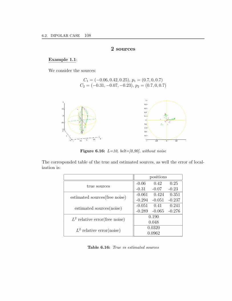
6.2. DIPOLAR CASE 108
2 sources
Example 1.1:
We consider the sources:
C1 = (−0.06, 0.42, 0.25), p1 = (0.7, 0, 0.7)C2 = (−0.31,−0.07,−0.23), p2 = (0.7, 0, 0.7)
Figure 6.16: L=10, belt=[0,90], without noise
The corresponded table of the true and estimated sources, as well the error of local-ization is:
positions
true sources-0.06 0.42 0.25-0.31 -0.07 -0.23
estimated sources(free noise)-0.061 0.424 0.351-0.294 -0.051 -0.237
estimated sources(noise)-0.051 0.41 0.241-0.289 -0.065 -0.276
L2 relative error(free noise)0.1900.048
L2 relative error(noise)0.03200.0962
Table 6.16: True vs estimated sources
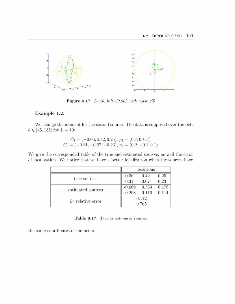
6.2. DIPOLAR CASE 109
Figure 6.17: L=10, belt=[0,90], with noise 2%
Example 1.2:
We change the moment for the second source. The data is supposed over the beltθ ∈ [45, 135] for L = 10:
C1 = (−0.06, 0.42, 0.25), p1 = (0.7, 0, 0.7)C2 = (−0.31,−0.07,−0.23), p2 = (0.2,−0.1, 0.1)
We give the corresponded table of the true and estimated sources, as well the errorof localization. We notice that we have a better localization when the sources have
positions
true sources-0.06 0.42 0.25-0.31 -0.07 -0.23
estimated sources-0.069 0.369 0.478-0.208 0.116 0.114
L2 relative error0.1420.765
Table 6.17: True vs estimated sources
the same coordinates of moments.
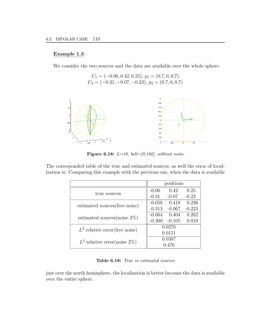
6.2. DIPOLAR CASE 110
Example 1.3:
We consider the two sources and the data are available over the whole sphere.
C1 = (−0.06, 0.42, 0.25), p1 = (0.7, 0, 0.7)C2 = (−0.31,−0.07,−0.23), p2 = (0.7, 0, 0.7)
Figure 6.18: L=10, belt=[0,180], without noise
The corresponded table of the true and estimated sources, as well the error of local-ization is: Comparing this example with the previous one, when the data is available
positions
true sources-0.06 0.42 0.25-0.31 -0.07 -0.23
estimated sources(free noise)-0.058 0.418 0.236-0.313 -0.067 -0.223
estimated sources(noise 2%)-0.064 0.404 0.262-0.300 -0.105 0.019
L2 relative error(free noise)0.02760.0151
L2 relative error(noise 2%)0.03870.476
Table 6.18: True vs estimated sources
just over the north hemisphere, the localization is better because the data is availableover the entire sphere.

6.2. DIPOLAR CASE 111
General remarks:
1. The bandwidth L plays an important role in the source localization: bigger theL is, smaller the error localization becomes.
2. The localization depends also on the positions of the sources with respect tothe belt, i.e. if the sources are placed or not in the covered region.
3. The localization is also improved when the data is considered over the wholesphere.

6.2. DIPOLAR CASE 112
Chapter7Conclusion
This thesis is developped around the representation of data on the sphere andapproximation, for transmission and recovery problems concerning some Laplacepartial differential equations.
The resolution of the associated inverse problems requires a first transmissiondata step, from the considered region to the whole boundary sphere, and in a secondtime, the recovery of the sources in the domain [17].
The use of families like spherical harmonics and Slepian bases is of special interestfor the resolution of such inverse problems in geodesy and EEG, when we dispose ofpartial boundary data.
When we dispose of different types of heterogeneous data, as the gravitationalpotential measured at the surface of the Earth and its derivative or Hessian measuredon sattelite orbits, for their expansion we can use different bases like Slepian [46],wavelets [13] or other functions families.
Suitable functions families here are given by Slepian bases that allow to representpartially available data on sphere, whenever these come from almost band-limitedfunctions (this is numerically the case; however, further error bounds should beestablished concerning the above potentials with pointwise or localized singularitiesin the ball, following Chapter 4). For the computation of such a Slepian basis, anefficient scheme has been proposed, using Gauss-Legendre quadrature methods [33].The comparison between zonal spherical harmonics and Slepian functions would beinteresting particularly when the studied region is a belt, contained between twoparallels of the sphere.
In practice, the nodes location is imposed (they are not chosen as suitable nodes,as for Gauss-Legendre quadrature) and consequently, the study of different quadra-ture methods (as points of a cubature rule on the sphere, see [49]) which could give
113
114
more flexibility on the choice of the nodes (location of electrodes or satellites) issuitable.
The considered data could be gravitational or electrical potential measured atpoints on the boundary sphere (from electrodes on the scalp, or by gravimeters onthe Earth surface) or some other sphere (for satellite measurements, or for MEG).
For the case when we dispose of partial data over particular regions of the sphere,the estimation of the data over all the sphere can be formulated in terms of bestconstrained approximation problems [5], boundary elements methods or other regu-larization techniques [17].
For the second sources recovery step of the inverse problem, from data now avail-able on a whole sphere, we used best quadratic rational approximation methods onplanar sections [8, 17]. It furnishes good localization results for monopolar and dipo-lar sources type. The source localization results could be improved using severaldirections of planar sections, technique called of "clustering". This procedure yieldsa family of estimations of the sources at the intersection of the axis [17].
Concerning EEG issues, simultaneous measurements from MEG could be used fora better source localization (this will be done through the software FindSources3D,[24]).
To complete the resolution of the inverse problem, masses and moments identifi-cation is further required [43].
Similar inverse problems come from other physical and non destructive controlissues, like paleomagnetism [7], determination of the thickness of glaciers and soils,exploration of subsoils, etc.

Bibliography
[1] A. Abdelmoula, M. Moakher, and B. Philippe, Localized spectral anal-ysis for an inverse problem in geodesy, CARI, (2008).
[2] A. Albertella, F. Anso, and N. Neeuw, Band-limited functions on abounded spherical domain: the Slepian problem on the sphere, Journal Geodesy,73 (1999), pp. 436–447.
[3] M. Alfaro, J. Dehesa, F. Marcellan, J. R. de Francia, and J. Vin-
uesa, Orthogonal Polynomials and their Applications, SIAM, 1988.
[4] G. Andrews, R. Askey, and R. Roy, Special functions, 2011.
[5] B. Atfeh, L. Baratchart, J. Leblond, and J. Partington, Boundedextremal and Cauchy-Laplace problems on the sphere and shell, The Journal ofFourier Analysis and Applications, 16 (2010), pp. 177–203.
[6] L. Baratchart, A. Ben Abda, F. Ben Hassen, and J. Leblond, Re-covery of pointwise sources or small inclusions in 2D domains and rationalapproximation, Inverse problems, 21 (2005), pp. 51–74.
[7] L. Baratchart, D. Hardin, E. Lima, E. Saff, and B. Weiss, Inversemagnetization problems for a two-dimensional slab and generalizations of hodgedecompositions, V Bell Syst. Tech. J., (30 September, 2011).
[8] L. Baratchart, J. Leblond, and J.-P. Marmorat, Inverse source prob-lem in a 3D ball from best meromorphic approximation on 2D slices, ETNA, 25(2006), pp. 41–53.
[9] L. Baratchart and M. Yattselev, Meromorphic approximants to complexCauchy transforms with polar singularities, Mat. Sb., 200 (2009), pp. 3–40.
115
BIBLIOGRAPHY 116
[10] F. Ben Hassen and E. Bonnetier, Asymptotic formulas for the voltagepotential in a composite medium containing close or touching disks of smalldiameter, Multiscale Model. Simul., 4 (2005), pp. 250–277.
[11] A. Bultheel and B. D. Moor, Rational approximation in linear systemand control, Journal of Computation and Applied Mathematics, 121 (2000),pp. 355–378.
[12] F. Chambat and Y. Ricard, Empirical 3D basis for the internal density ofa planet, Geophysical Journal International, 162 (2005), pp. 32–35.
[13] A. Chambodut, I. Panet, M. Mandea, D. Diament, M. Holschnei-
der, and O. Jamet, Wavelet frames: an alternative to spherical harmonicrepresentation of potential fields, Geophys. J. Int., 163 (2005), pp. 857–899.
[14] G. Chen and J. Zhou, Boundary element methods, Academic Press London,1992.
[15] M. Chung, K. Dalton, A. Evans, and R. Davidson, Tensor-based corti-cal surface morphometry via weighted spherical harmonic representation, IEEE.Trans. Med. Imag., (2007).
[16] S. Claessens, W. Featherstone, and F. Barthelmes, Experiences withpoint-mass gravity field modelling in the Perth region, Geomatics Research Aus-tralasia, 75 (2001), pp. 53–86.
[17] M. Clerc, J.Leblond, J.-P. Marmorat, and T. Papadopoulo, Sourcelocalization using rational approximation on plane sections. Research Report,submitted, 2011.
[18] B. Cuffin, A method for localizing EEG sources in realistic head models, IEEETransBiomed Eng., 42 (1995), pp. 68–71.
[19] R. Dautray and J. Lions, Analyse Mathématique et Calcul Numerique pourles Sciences et les techniques, vol. 3, Masson, 1988.
[20] P. Davis and P. Rabinowitz, Methods of Numerical Integration, AcademicPress Inc, second ed., 1984.
[21] A. El Badia, Summary of some results on an EEG inverse problem, Neurologyand Clinical Neurophysiology, 104 (2004).
BIBLIOGRAPHY 117
[22] A. El Badia and T. Duong, An inverse source problem in potential analysis,Inverse Problems, 16 (2000), pp. 651–663.
[23] A. El Badia and M. Farah, A stable recovering of dipole sources from partialboundary measurements, Inverse Problems, 26 (2010).
[24] FindSources3D, Guide utilisateur, url: http://www-sop.inria.fr/apics/FindSources3D, INRIA, APICS-ATHENA, 2009.
[25] A. Friedman and M. Vogelius, Identification of small inhomogeneities ofextreme conductivity by boundary measurements: a theorem on continuous de-pendence, Arch. Rat. Mech. Anal., 105 (1989), pp. 299–326.
[26] E. Gilbert and D. Slepian, Existence and generic properties of l2 approxi-mants of linear systems, IMA Journal of Mathematical Control and Information,3 (1986), pp. 89–101.
[27] K. Gorski, E. Hivon, A. Banday, B. Wandelt, F. Hansen, M. Rei-
necke, and M. Bantelman, A framework for high-resolution discretizationand fast analysis of data distributed on the sphere, Astroph. J., 622 (2005),pp. 759–771.
[28] R. Gregory, Uniform bounds for Pmn (cos θ) and the absolute convergence of
series expansions in spherical surface harmonics, Quartely Journal of Mechanicsand Applied Mathematics, 50 (1997), pp. 467–479.
[29] V. Isakov, Inverse problems for partial differential equations, Springer-Verlag,Berlin, 1998.
[30] J. Jackson, Classical Electrodynamics, Academic Press Inc, third ed., 1984.
[31] K. Jerbi, J. Mosher, S. Baillet, and R. Leahy, On MEG forward mod-elling using multipolar expansions, Physics in Medicine and Biology, 47 (2002),pp. 523–555.
[32] A. Karoui, Recent developments in fractals and related fields. Based on theinternational conference on fractals and related fields, Uncertainty principles,prolate spheroidal wave functions, and applications, Springer Science+BusinessMedia, 2010.
[33] A. Karoui, J. Leblond, and A.-M. Nicu, Slepian functions on the spherewith applications to signal recovery and inverse source problems, in preparation,(2012).
BIBLIOGRAPHY 118
[34] J. Keiner and D. Potts, Fast evaluation of quadrature formulae on thesphere, Mathematics and Computation, 77 (2008), pp. 397–419.
[35] A. Krall, Hilbert Space Boundary Value Problems and Orthogonal Polynomi-als, Birkhauser Verlag, 2002.
[36] H. Landau and H. Pollak, Prolate spheroidal wave functions, Fourier anal-ysis and uncertainty ii, Bell Syst. Tech. Journal., 40 (1961), pp. 65–84.
[37] J. Marmorat and M. Olivi, The RARL2 software: Realiza-tions and Rational Approximation in L2-norm, url: http://www-sop.inria.fr/apics/RARL2/rarl2-eng.html, Project APICS, INRIA, SophiaAntipolis.
[38] V. Michel, Regularized wavelet-based multiresolution recovery of the harmonicmass density distribution from data of the Earth’s gravitational field at satelliteheight, Inverse problems, 21 (2005).
[39] V. Michel and A. Fokas, A unified approach to various techniques for thenon- uniqueness of the inverse gravimetric problem and wavelet-based methods,Inverse problems, 24 (2008).
[40] L. Miranian, Slepian functions on the sphere, generalized Gaussian quadraturerule, Inverse Problems, 20 (2004).
[41] J. Mosher, P. Lewis, and R. Leahy, Multiple dipole modelling and localiz-ing from spatio-temporal meg data, IEEE Transactions on Biomedical Engineer-ing, 39 (1992), pp. 541–553.
[42] A. Nikiforov, Special functions of mathematical physics, Birkhauser BerlagBasel, 1988.
[43] H. Ouerghi, Localization des sources ponctuelle dans une boule par approxi-mation sur les sections planes: calcules des moments, Master’s thesis, Tunis,Tunisie, 2008.
[44] W. Rudin, Analyse réelle et complexe, Masson, 1975.
[45] J. Sarvas, Basic mathematical and electromagnetic concepts of the biomagneticinverse problem, Physics in Medicine and Biology, 32 (1987), pp. 11–12.
[46] F. Simons and F. Dahlen, Spherical Slepian functions and the polar gap ingeodesy, Geophysics Journal, 166 (2006), pp. 1039–1061.
BIBLIOGRAPHY 119
[47] F. Simons, F. Dahlen, and M. Wieczorek, Spatiospectral concentrationon a sphere, SIAM, 48 (2006), pp. 504–536.
[48] D. Slepian, Prolate spheroidal wave functions, fourier analysis and uncer-tainty, V Bell Syst. Tech. J., 57 (1978), pp. 1371–430.
[49] I. Sloan and R. Womersley, Good approximation on the sphere, with ap-plication to geodesy and the scattering of sound, Journal of Computational andApplied Mathematics, 149 (2002), pp. 227–237.
[50] N. Sneeuw and M. van Gelderen, The polar gap, vol. 65, Springer, 1997,pp. 559–568.
[51] D. Stromeyer and L. Ballani, Uniqueness of the inverse gravimetric prob-lem for point mass models, Manuscr. Geodaet., 9 (1984), pp. 125–136.
[52] G. Szegö, Orthogonal polynomials, American Mathematical Society Collo-quium Publications, Vol. 23. Revised ed, American Mathematical Society, 1959.
[53] S. Vessella, Locations and strengths of point sources: Stability estimates, In-verse Problems, 8 (1992), pp. 911–917.
[54] B. Wellenhof and H. Moritz, Physical geodesy, Springer-Verlag, Wien,second ed., 2006.
[55] N. Young, An introduction to Hilbert space, Cambridge Mathematical text-books, (1998).
[56] M. Zghal, Problèmes inverses pour l’équation de Laplace en dimension 3:Application à l’électroencéphalographie, PhD thesis, ENIT LAMSIN, Tunis,Tunisie, 2010.

BIBLIOGRAPHY 120
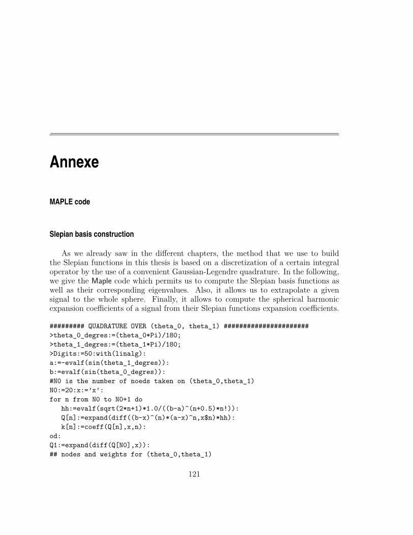
Annexe
MAPLE code
Slepian basis construction
As we already saw in the different chapters, the method that we use to buildthe Slepian functions in this thesis is based on a discretization of a certain integraloperator by the use of a convenient Gaussian-Legendre quadrature. In the following,we give the Maple code which permits us to compute the Slepian basis functions aswell as their corresponding eigenvalues. Also, it allows us to extrapolate a givensignal to the whole sphere. Finally, it allows to compute the spherical harmonicexpansion coefficients of a signal from their Slepian functions expansion coefficients.
######### QUADRATURE OVER (theta_0, theta_1) ######################
>theta_0_degres:=(theta_0*Pi)/180;
>theta_1_degres:=(theta_1*Pi)/180;
>Digits:=50:with(linalg):
a:=-evalf(sin(theta_1_degres)):
b:=evalf(sin(theta_0_degres)):
#N0 is the number of noeds taken on (theta_0,theta_1)
N0:=20:x:=’x’:
for n from N0 to N0+1 do
hh:=evalf(sqrt(2*n+1)*1.0/((b-a)^(n+0.5)*n!)):
Q[n]:=expand(diff((b-x)^(n)*(a-x)^n,x$n)*hh):
k[n]:=coeff(Q[n],x,n):
od:
Q1:=expand(diff(Q[N0],x)):
## nodes and weights for (theta_0,theta_1)
121
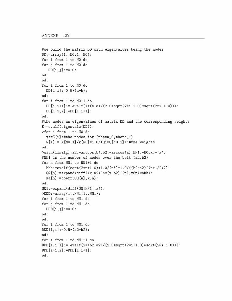
ANNEXE 122
#we build the matrix DD with eigenvalues being the nodes
DD:=array(1..N0,1..N0):
for i from 1 to N0 do
for j from 1 to N0 do
DD[i,j]:=0.0:
od:
od:
for i from 1 to N0 do
DD[i,i]:=0.5*(a+b):
od:
for i from 1 to N0-1 do
DD[i,i+1]:=-evalf(i*(b-a)/(2.0*sqrt(2*i+1.0)*sqrt(2*i-1.0))):
DD[i+1,i]:=DD[i,i+1]:
od:
#the nodes as eigenvalues of matrix DD and the corresponding weights
E:=evalf(eigenvals(DD)):
>for i from 1 to N0 do
x:=E[i]:#the nodes for (theta_0,theta_1)
W[i]:=-k[N0+1]/k[N0]*1.0/(Q1*Q[N0+1]):#the weights
od:
>with(linalg):a2:=arccos(b):b2:=arccos(a):NN1:=N0:x:=’x’:
#NN1 is the number of nodes over the belt (a2,b2)
for n from NN1 to NN1+1 do
hhh:=evalf(sqrt(2*n+1.0)*1.0/(n!)*1.0/((b2-a2)^(n+1/2))):
QQ[n]:=expand(diff((x-a2)^n*(x-b2)^(n),x$n)*hhh):
ka[n]:=coeff(QQ[n],x,n):
od:
QQ1:=expand(diff(QQ[NN1],x)):
>DDD:=array(1..NN1,1..NN1):
for i from 1 to NN1 do
for j from 1 to NN1 do
DDD[i,j]:=0.0:
od:
od:
for i from 1 to NN1 do
DDD[i,i]:=0.5*(a2+b2):
od:
for i from 1 to NN1-1 do
DDD[i,i+1]:=-evalf(i*(b2-a2)/(2.0*sqrt(2*i+1.0)*sqrt(2*i-1.0))):
DDD[i+1,i]:=DDD[i,i+1]:
od:
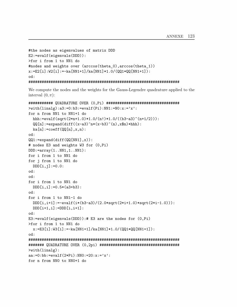
ANNEXE 123
#the nodes as eigenvalues of matrix DDD
E2:=evalf(eigenvals(DDD)):
>for i from 1 to NN1 do
#nodes and weights over (arccos(theta_0),arccos(theta_1))
x:=E2[i]:W2[i]:=-ka[NN1+1]/ka[NN1]*1.0/(QQ1*QQ[NN1+1]):
od:
####################################################################
We compute the nodes and the weights for the Gauss-Legendre quadrature applied to theinterval (0, π):
########### QUADRATURE OVER (0,Pi) #################################
>with(linalg):a3:=0:b3:=evalf(Pi):NN1:=N0:x:=’x’:
for n from NN1 to NN1+1 do
hhh:=evalf(sqrt(2*n+1.0)*1.0/(n!)*1.0/((b3-a3)^(n+1/2))):
QQ[n]:=expand(diff((x-a3)^n*(x-b3)^(n),x$n)*hhh):
ka[n]:=coeff(QQ[n],x,n):
od:
QQ1:=expand(diff(QQ[NN1],x)):
# nodes E3 and weights W3 for (0,Pi)
DDD:=array(1..NN1,1..NN1):
for i from 1 to NN1 do
for j from 1 to NN1 do
DDD[i,j]:=0.0:
od:
od:
for i from 1 to NN1 do
DDD[i,i]:=0.5*(a3+b3):
od:
for i from 1 to NN1-1 do
DDD[i,i+1]:=-evalf(i*(b3-a3)/(2.0*sqrt(2*i+1.0)*sqrt(2*i-1.0))):
DDD[i+1,i]:=DDD[i,i+1]:
od:
E3:=evalf(eigenvals(DDD)):# E3 are the nodes for (0,Pi)
>for i from 1 to NN1 do
x:=E3[i]:W3[i]:=-ka[NN1+1]/ka[NN1]*1.0/(QQ1*QQ[NN1+1]):
od:
####################################################################
####### QUADRATURE OVER (0,2pi) ####################################
>with(linalg):
aa:=0:bb:=evalf(2*Pi):NN0:=20:x:=’x’:
for n from NN0 to NN0+1 do
ANNEXE 124
hhh:=evalf(sqrt(2*n+1.0)*1.0/(n!)*1.0/(bb^(n+1/2))):
QQ[n]:=expand(diff(x^n*(x-bb)^(n),x$n)*hhh):
ka[n]:=coeff(QQ[n],x,n):
od:
QQ1:=expand(diff(QQ[NN0],x)):
# nodes EE and weights WW for (0,2PI)
DDD:=array(1..NN0,1..NN0):
for i from 1 to NN0 do
for j from 1 to NN0 do
DDD[i,j]:=0.0:
od:od:
for i from 1 to NN0 do
DDD[i,i]:=0.5*(aa+bb):
od:
for i from 1 to NN0-1 do
DDD[i,i+1]:=-evalf(i*(bb-aa)/(2.0*sqrt(2*i+1.0)*sqrt(2*i-1.0))):
DDD[i+1,i]:=DDD[i,i+1]:
od:
EE:=evalf(eigenvals(DDD)):
#### nodes and weights ######
>for i from 1 to NN0 do
x:=EE[i]:
WW[i]:=-ka[NN0+1]/ka[NN0]*1.0/(QQ1*QQ[NN0+1]):
od:
###################################################################
We compute the kernel of the operator Tmassociated to Slepian functions
######### KERNEL K(m,x,y) #######################################
>x:=’x’:y:=’y’:
>K:=proc(m,x,y)
if (m=0) then evalf(sum((2*l+1.0)/(4.0*Pi)*1/(2^l*l!)
*(diff((x^2-1)^l,x$l))*1/(2^l*l!)*(diff((y^2-1)^l,y$l)),l=0..L)):
else
evalf(sum((2*l+1.0)/(4.0*Pi)*(((l-abs(m))!)/((l+abs(m))!)
*((1-x^2)^(m/2)*1/(2^l*l!)*diff(diff((x^2-1)^l,x$l),x$m)
*(1-y^2)^(m/2)*1/(2^l*l!)*diff(diff((y^2-1)^l,y$l),y$m))),l=abs(m)..L)):
fi:
end:
###################################################################
Using the quadrature Gauss-Legendre over the belt (θ0, θ1), we compute the eigenvaluesand eigenfunctions of the kerner K(m, x, y) evaluated at the nodes taken over the belt:
ANNEXE 125
######## EIGENVALUES of K(m,x,y) #################################
>with(LinearAlgebra):mmm:=’mmm’:mmm:=L+1:i:=0:j:=0:
A:=Matrix(1..mmm*N0,1..N0):
for m from 0 to mmm-1 do
for i from 1 to N0 do
for j from 1 to N0 do
A[m*N0+i,j]:=evalf(W[j]*subs(x=E[i],y=E[j],K(m,x,y))):x:=’x’:y:=’y’:
#we evaluate the kernel in the nodes "E" taken over the belt
od:od:od:
m:=’m’:
for m from 0 to mmm-1 do
F[m]:=eigenvectors(SubMatrix(A,[m*N0+1..(m+1)*N0],[1..N0])):
od:
###################################################################
######## SORTED EIGENVALUES #######################################
#here, we sort ascending the eignevalues
beta:=Matrix(1..mmm,1..N0):
for m from 0 to mmm-1 do
for p from 1 to N0 do
beta[m+1,p]:=abs(F[m][p][1]):
od:od:
for m from 0 to mmm-1 do
X[m]:=Row(beta,m+1):Xsort[m]:=sort(X[m]):
od:
###################################################################
######## EIGENVALUES READING ###################################
>for m from 0 to mmm-1 do
for mm from 1 to N0 do
R[m,mm]:=0:
od:od:
for m from 0 to mmm-1 do
for i from 1 to N0 do
for j from 1 to N0 do
if((abs(Xsort[m][i])-abs(F[m][j][1]))=0) then R[m,i]:=j:
else R[m,j]:=R[m,j]+0:
fi:
od:od:od:
###################################################################
The approximate eigenfunctions of the integral operator with the kernel K(m, x, y) byusing Gauss-Legendre quadrature over the belt (θ0, θ1):
ANNEXE 126
########## EIGENFUNCTIONS #########################################
>n:=’n’:m:=’m’:
>psi:=proc(n,m,x)
evalf((1.0/F[m][R[m,N0+1-n]][1])*sum(W[kk]*subs(y=E[kk],K(m,x,y))
*F[m][R[m,N0+1-n]][3][1][kk],kk=1..N0)):
end:
###################################################################
Multiplying the eigenfunctions of the operator K(m, x, y) by eimφ, we compute the Slepianfunctions.
## NORMALIZATION CONSTANTE BY USING GAUSS-LEGENDRE QUADRATURE ##
>kk:=’kk’:
for m from 0 to mmm-1 do
for n from 1 to (L-m+1) do
AA[n,m]:=evalf(sum(W[kk]*(F[m][R[m,N0+1-n]][3][1][kk])^2, kk=1..N0)):
od:od:
ppsi:=proc(n,m,x)
evalf((1.0/sqrt(AA[n,m])*psi(n,m,x))):
end:
subs(x=3,ppsi(2,1,x));
####################################################################
######## NORMALIZED SLEPIAN FUNCTIONS ##############################
>slepian:=proc(n,m,theta,phi)
if (m<=L-1) then if(n<=L-m+1) then subs(x=cos(theta),
evalf(1.0/sqrt(evalf(Pi)))*ppsi(n,m,x))*cos(m*phi)
else
subs(x=cos(theta),evalf(1.0/sqrt(evalf(Pi)))*ppsi(n-L+m-1,m,x))*sin(m*phi)
fi:
else
if(m=L) then
if(n=1) then
subs(x=cos(theta), evalf(1.0/sqrt(evalf(Pi)))*ppsi(1,L,x))*cos(L*phi)
else
subs(x=cos(theta),evalf(1.0/sqrt(evalf(Pi)))*ppsi(1,L,x))*sin(L*phi)
fi:
fi:
fi:
end:
####################################################################
We indroduce the matrix whose coefficients are the Slepian functions evaluated at thequadrature nodes:
ANNEXE 127
# MATRIX T COMPUTATION WHOSE COEFFICIENTS ARE SLEPIAN FUNCTIONS ####
>T:=Matrix((L+1)*(L+2),N0*NN0):
iii:=0:
for m from 0 to L do
for n from 1 to 2*(L-m+1) do
iii:=iii+1:jjj:=0:
for k from 1 to N0 do
for j from 1 to NN0 do:
jjj:=jjj+1:T[iii,jjj]:=evalf(WW[j]*W2[k]*sin(E2[k])
*slepian(n,m,E2[k],EE[j])):
od:od:
od:od:
#here, we put away zero slepian functions (for m=0 n=L+1..2*(L+m+1))##
T2:=Matrix((L+1)^2,N0*NN0):jjj:=0:
for k from 1 to N0 do
for j from 1 to NN0 do
jjj:=jjj+1:T2[1..L+1,jjj]:=T[1..L+1,jjj]:T2[L+2..(L+1)^2,jjj]
:=T[2*(L+1)+
1..(L+1)*(L+2),jjj]:
od:
od;
######################################################################
By using this matrix, we compute the Slepian functions expansion coefficients ofa given signal. By a matrix multiplication between the matrix T and the matrixassociated to the signal (potential) computed in the nodes taken on the belt we getthe coefficients. After having the Slepian functions and the coefficients, we can givethe expansion of the signal over the sphere. Moreover, from this expansion we canget the spherical harmonic expansion coefficients of the signal. In the following,we consider as application a particular signal, the gravitational potential, and wegive the code for the previous scheme. Note that the input data (the bandwith, thepositions of sources, the angels which parametrize the belt) is given in a file which wecall data.txt. The file will be opened for reading the data using basical file commands.
Spherical harmonic coefficients of a potential generated by a monopolar and dipolar sourcesdistribution
\section
##################### READ DATA ####################################
>Restart;_EnvLegendreCut := 1 .. infinity;forget(evalf);
ANNEXE 128
># we give the name of the input file
>name_file_to_read:=readstat("The name of the file");
>convert(name_file_to_read,string);
>#here, we open the file for reading the data
>f:=fopen("../datafiles/"||name_file_to_read||"."||txt,READ,TEXT);
>#we read each line
>i:=0:while ligne[i]<>0 do i:=i+1:ligne[i]:=readline(f) end do:fclose(f):
Ligne:=convert(ligne,list);whattype(Ligne);nops(Ligne):
>i:=0:
for i from 1 to nops(Ligne) do
if Ligne[i]="# BELT"
then t:=sscanf(Ligne[i+1], "%d%d"):
theta_0:=t[1]:theta_1:=t[2]:position_belt:=i:
fi:
if Ligne[i]="# BANDWITH"
then L0:=sscanf(Ligne[i+1], "%d");
L:=L0[1]:
fi:
if Ligne[i]="# SOURCES"
then
position_source:=i:
fi:
od:
>nbSources:=position_belt-position_source-1:
source:=Array(1..nbSources,1..4):j:=0:
for j from 1 to nbSources do
s[j]:=sscanf(Ligne[position_source+j], "%f%f%f%f");
source[j,1]:=s[j][1];
source[j,2]:=s[j][2];
source[j,3]:=s[j][3]:
source[j,4]:=s[j][4]:
od:
########################################################################
We compute the real spherical harmonic basis:
############# SPHERICAL HARMONIC BASIS CONSTRUCTION ####################
>Y2:=proc(l,m,x,y)
evalf(sqrt(2*(2*l+1)/(4*Pi)*(l-abs(m))!/(l+abs(m))!)
*LegendreP(l,abs(m),x)*cos(m*y)):
end:
Y1:=proc(l,m,x,y)
ANNEXE 129
evalf(sqrt(2*(2*l+1)/(4*Pi)*(l-abs(m))!/(l+abs(m))!)
*LegendreP(l,abs(m),x)*sin(m*y)):
end:
Y3:=proc(l,m,x,y)
evalf(sqrt((2*l+1)/(4*Pi)))*(l-0)/(l+0)*diff(1/(2^l*l!)*(1-x^2)^l,x$l):
end:
Y:=proc(l,m,x,y)
if m>0 then Y2(l,m,x,y)
elif m<0 then Y1(l,m,x,y)
elif m=0 then Y3(l,m,x,y)
fi:
end:
###########################################################################
################ QUADRATURE OVER (theta_0, theta_1) #######################
>theta_0_degres:=(theta_0*Pi)/180;
>theta_1_degres:=(theta_1*Pi)/180;
>Digits:=50:with(linalg):
a:=-evalf(sin(theta_1_degres)):
b:=evalf(sin(theta_0_degres)):
N0:=20:x:=’x’:
for n from N0 to N0+1 do
hh:=evalf(sqrt(2*n+1)*1.0/((b-a)^(n+0.5)*n!)):
Q[n]:=expand(diff((b-x)^(n)*(a-x)^n,x$n)*hh):
k[n]:=coeff(Q[n],x,n):
od:
Q1:=expand(diff(Q[N0],x)):
#######the zeros of P_n as eigenvalues of DD matrix ###############
DD:=array(1..N0,1..N0):
for i from 1 to N0 do
for j from 1 to N0 do
DD[i,j]:=0.0:
od:
od:
for i from 1 to N0 do
DD[i,i]:=0.5*(a+b):
od:
for i from 1 to N0-1 do
DD[i,i+1]:=-evalf(i*(b-a)/(2.0*sqrt(2*i+1.0)*sqrt(2*i-1.0))):
DD[i+1,i]:=DD[i,i+1]:
od:
E:=evalf(eigenvals(DD)):
ANNEXE 130
####### nodes and weights #######################################
>for i from 1 to N0 do
x:=E[i]:#the nodes
W[i]:=-k[N0+1]/k[N0]*1.0/(Q1*Q[N0+1]):#the weights
od:
>with(linalg):a2:=arccos(b):b2:=arccos(a):NN1:=N0:x:=’x’:
for n from NN1 to NN1+1 do
hhh:=evalf(sqrt(2*n+1.0)*1.0/(n!)*1.0/((b2-a2)^(n+1/2))):
QQ[n]:=expand(diff((x-a2)^n*(x-b2)^(n),x$n)*hhh):
ka[n]:=coeff(QQ[n],x,n):
od:
QQ1:=expand(diff(QQ[NN1],x)):
>DDD:=array(1..NN1,1..NN1):
for i from 1 to NN1 do
for j from 1 to NN1 do
DDD[i,j]:=0.0:
od:
od:
for i from 1 to NN1 do
DDD[i,i]:=0.5*(a2+b2):
od:
for i from 1 to NN1-1 do
DDD[i,i+1]:=-evalf(i*(b2-a2)/(2.0*sqrt(2*i+1.0)*sqrt(2*i-1.0))):
DDD[i+1,i]:=DDD[i,i+1]:
od:
E2:=evalf(eigenvals(DDD)):
>for i from 1 to NN1 do
x:=E2[i]:W2[i]:=-ka[NN1+1]/ka[NN1]*1.0/(QQ1*QQ[NN1+1]): #nodes and weights
od:
############################################################################
########### QUADRATURE OVER (0,Pi) #########################################
>with(linalg):a3:=0:b3:=evalf(Pi):NN1:=N0:x:=’x’:
for n from NN1 to NN1+1 do
hhh:=evalf(sqrt(2*n+1.0)*1.0/(n!)*1.0/((b3-a3)^(n+1/2))):
QQ[n]:=expand(diff((x-a3)^n*(x-b3)^(n),x$n)*hhh):
ka[n]:=coeff(QQ[n],x,n):
od:
QQ1:=expand(diff(QQ[NN1],x)):
DDD:=array(1..NN1,1..NN1):
for i from 1 to NN1 do
for j from 1 to NN1 do
ANNEXE 131
DDD[i,j]:=0.0:
od:
od:
for i from 1 to NN1 do
DDD[i,i]:=0.5*(a3+b3):
od:
for i from 1 to NN1-1 do
DDD[i,i+1]:=-evalf(i*(b3-a3)/(2.0*sqrt(2*i+1.0)*sqrt(2*i-1.0))):
DDD[i+1,i]:=DDD[i,i+1]:
od:
E3:=evalf(eigenvals(DDD)):
# nodes and weights
>for i from 1 to NN1 do
x:=E3[i]:W3[i]:=-ka[NN1+1]/ka[NN1]*1.0/(QQ1*QQ[NN1+1]):
od:
###########################################################################
########## QUADRATURE OVER (0,2pi) ########################################
>with(linalg):
aa:=0:bb:=evalf(2*Pi):NN0:=20:x:=’x’:
for n from NN0 to NN0+1 do
hhh:=evalf(sqrt(2*n+1.0)*1.0/(n!)*1.0/(bb^(n+1/2))):
QQ[n]:=expand(diff(x^n*(x-bb)^(n),x$n)*hhh):
ka[n]:=coeff(QQ[n],x,n):
od:
QQ1:=expand(diff(QQ[NN0],x)):
les zeros du P_n comme des valeurs propres de la matrice DDD
DDD:=array(1..NN0,1..NN0):
for i from 1 to NN0 do
for j from 1 to NN0 do
DDD[i,j]:=0.0:
od:od:
for i from 1 to NN0 do
DDD[i,i]:=0.5*(aa+bb):
od:
for i from 1 to NN0-1 do
DDD[i,i+1]:=-evalf(i*(bb-aa)/(2.0*sqrt(2*i+1.0)*sqrt(2*i-1.0))):
DDD[i+1,i]:=DDD[i,i+1]:
od:
EE:=evalf(eigenvals(DDD)):
#### nodes and weights ######
>for i from 1 to NN0 do

ANNEXE 132
x:=EE[i]:
WW[i]:=-ka[NN0+1]/ka[NN0]*1.0/(QQ1*QQ[NN0+1]):
od:
#####################################################################
######### KERNEL K(m,x,y) ##########################################
>x:=’x’:y:=’y’:
>K:=proc(m,x,y)
if (m=0) then evalf(sum((2*l+1.0)/(4.0*Pi)*1/(2^l*l!)
*(diff((x^2-1)^l,x$l))*1/(2^l*l!)*(diff((y^2-1)^l,y$l)),l=0..L)):
else
evalf(sum((2*l+1.0)/(4.0*Pi)*(((l-abs(m))!)/((l+abs(m))!)
*((1-x^2)^(m/2)*1/(2^l*l!)*diff(diff((x^2-1)^l,x$l),x$m)
*(1-y^2)^(m/2)*1/(2^l*l!)*diff(diff((y^2-1)^l,y$l),y$m))),l=abs(m)..L)):
fi:
end:
####################################################################
######## EIGENVALUES of K(m,x,y) ###################################
>#the eigenvalues of K which is computed in nodes taken over the belt:
>with(LinearAlgebra):mmm:=’mmm’:mmm:=L+1:i:=0:j:=0:
A:=Matrix(1..mmm*N0,1..N0):
for m from 0 to mmm-1 do
for i from 1 to N0 do
for j from 1 to N0 do
A[m*N0+i,j]:=evalf(W[j]*subs(x=E[i],y=E[j],K(m,x,y))):x:=’x’:y:=’y’:
od:od:od:
m:=’m’:
for m from 0 to mmm-1 do
F[m]:=eigenvectors(SubMatrix(A,[m*N0+1..(m+1)*N0],[1..N0])):
od:
#####################################################################
######## SORTED EIGENVALUES #########################################
>ascendent sorted eigenvalues
>beta:=Matrix(1..mmm,1..N0):
for m from 0 to mmm-1 do
for p from 1 to N0 do
beta[m+1,p]:=abs(F[m][p][1]):
od:od:
for m from 0 to mmm-1 do
X[m]:=Row(beta,m+1):Xsort[m]:=sort(X[m]):
od:
#####################################################################
ANNEXE 133
######## EIGENVALUES INDEXATION #####################################
>for m from 0 to mmm-1 do
for mm from 1 to N0 do
R[m,mm]:=0:
od:od:
for m from 0 to mmm-1 do
for i from 1 to N0 do
for j from 1 to N0 do
if((abs(Xsort[m][i])-abs(F[m][j][1]))=0) then R[m,i]:=j:
else R[m,j]:=R[m,j]+0:
fi:
od:od:od:
###########################################################################
######### EIGENFUNCTIONS OF THE KERNEL K(m,x,y)############################
#E are the nodes over the belt, W the weights of G-L quadrature of the belt
>n:=’n’:m:=’m’:
>psi:=proc(n,m,x)
evalf((1.0/F[m][R[m,N0+1-n]][1])*sum(W[kk]*subs(y=E[kk],K(m,x,y))
*F[m][R[m,N0+1-n]][3][1][kk],kk=1..N0)):
end:
###########################################################################
##### NORMALIZATION CONSTANTE OF GAUSS-LEGENDRE QUADRATURE ###############
>kk:=’kk’:
for m from 0 to mmm-1 do
for n from 1 to (L-m+1) do
AA[n,m]:=evalf(sum(W[kk]*(F[m][R[m,N0+1-n]][3][1][kk])^2, kk=1..N0)):
od:od:
ppsi:=proc(n,m,x)
evalf((1.0/sqrt(AA[n,m])*psi(n,m,x))):
end:
subs(x=3,ppsi(2,1,x));
########################################################################
######## NORMALIZED SLEPIAN FUNCTIONS ##################################
#From eigenfunctions of K(m,x,y), we build the slepian functions
>slepian:=proc(n,m,theta,phi)
if (m<=L-1) then if(n<=L-m+1) then subs(x=cos(theta),
evalf(1.0/sqrt(evalf(Pi)))*ppsi(n,m,x))*cos(m*phi)
else
subs(x=cos(theta),evalf(1.0/sqrt(evalf(Pi)))*ppsi(n-L+m-1,m,x))*sin(m*phi)
fi:
else
ANNEXE 134
if(m=L) then
if(n=1) then
subs(x=cos(theta), evalf(1.0/sqrt(evalf(Pi)))*ppsi(1,L,x))*cos(L*phi)
else
subs(x=cos(theta),evalf(1.0/sqrt(evalf(Pi)))*ppsi(1,L,x))*sin(L*phi)
fi:
fi:
fi:
end:
########################################################################
#EIGENVALUES COMPUTATION OF EIGENVALUES lambda[m,n],m=0..L,n=1..2(L-m+1)#
ASSOCIATED TO SLEPIAN FUNCTIONS slepian(n,m,theta,phi)
> m := 0;
for n to L+1 do
lambda[m, n] := evalf(2.0*Pi)*F[m][R[m, N0+1-n]][1]
od;
for m to L do
for n to L-m+1 do
lambda[m, n] := evalf(2.0*Pi)*F[m][R[m, N0+1-n]][1]
od;
for n from L-m+2 to 2*(L-m+1) do
lambda[m, n] := lambda[m, n-L+m-1]
od:od
##########################################################################
####### PLOT THE EIGENVALUES #############################################
>lambda1:=Vector(1..(L+1)^2):i:=0:m:=0:
for n from 1 to (L+1) do
i:=i+1:
lambda1[i]:= evalf(2.0*Pi)*F[m][R[m,N0+1-n]][1]:
od:
i:=0:
for m from 1 to L do
for n from 1 to (L-m+1) do
i:=i+1:lambda1[(L+1)+L*(L+1)/2+i]:=evalf(2.0*Pi)*F[m][R[m,N0+1-n]][1]:
lambda1[L+1+i]:=evalf(2.0*Pi)*F[m][R[m,N0+1-n]][1]:
od:
od:
k:=0:
for k from 1 to (L+1)^2 do
lambda1[k]
od:
ANNEXE 135
P:=sort(lambda1,‘>‘):
k:=0:
for k from 1 to (L+1)^2 do
P[k]
od:
plot([seq([k,P[k]],k=1..(L+1)^2)],style=point,color=red):
##########################################################################
########### PLOT THE EIGENVALUES #########################################
> plot(ppsi(1,3,x), x=0..1):
##########################################################################
######## PLOT THE SLEPIAN FUNCTIONS ######################################
>Slepian:=proc(n,m,theta,Phi)
evalf(subs(x=cos(theta),ppsi(n,m,x))*cos(m*phi)):
end;
plot3d(Slepian(1, 3, theta, Phi),theta = 0..evalf(Pi),phi = 0..evalf(2*Pi)):
##########################################################################
####### MATRIX T-COMPUTATION WHOSE COEFFICIENTS ARE SLEPIAN FUNCTIONS ####
>T:=Matrix((L+1)*(L+2),N0*NN0):
iii:=0:
for m from 0 to L do
for n from 1 to 2*(L-m+1) do
iii:=iii+1:jjj:=0:
for k from 1 to N0 do
for j from 1 to NN0 do:
jjj:=jjj+1:T[iii,jjj]:=evalf(WW[j]*W2[k]*sin(E2[k])*slepian(n,m,E2[k],EE[j])):
od:od:
od:od:
## here, we put away zero slepian functions (for m=0 n=L+1..2*(L+m+1)) ####
T2:=Matrix((L+1)^2,N0*NN0):jjj:=0:
for k from 1 to N0 do
for j from 1 to NN0 do
jjj:=jjj+1:T2[1..L+1,jjj]:=T[1..L+1,jjj]:T2[L+2..(L+1)^2,jjj]
:=T[2*(L+1)+1..(L+1)*(L+2), jjj]:
od:
od;
####################################################################
We give the bandlimited spherical harmonic developpement of the gravitational potential:
### GRAVITATIONAL POTENTIAL ########################################
>pot_monopolar:=proc(theta,phi)
i:=0:a3:=0:
ANNEXE 136
for i from 1 to nbSources do
a3:=a3+evalf(source[i,4]): od:
for i from 1 to nbSources do
for n from 1 to L do
for m from -n to n do
a3:=a3+evalf(source[i,4]*source[i,1]^n*((4*evalf(Pi))/(2*n+1))
*subs(x=cos(source[i,2]),y=source[i,3],Y(n,m,x,y))
*subs(x=cos(theta),y=phi,Y(n,m,x,y))):
od:od:od:
end;
#####################################################################
We compute the potential in the nodes taken over the belt and we associate the corre-sponded matrix:
########## THE POTENTIAL MATRIX ASSOCIATED ##########################
>S1:=Matrix(N0*NN0,3):jjj:=0:
for k from 1 to N0 do
for j from 1 to NN0 do
jjj:=jjj+1:
S1[jjj,1]:=pot_monopolar((E2[k]),EE[j]):
S1[jjj,2]:=E2[k]:
S1[jjj,3]:=EE[j]:
od:
od:
>s1:=array(1..N0*NN0): ## the potential array
for i from 1 to N0*NN0 do
s1[i]:= S1[i,1]:
od:
########################################################################
We compute the coefficients of the potential developpement on Slepian basis:
###### THE COEFFS OF THE SLEPIAN POTENTIAL DEVELOPEMENT ################
>C1:=multiply(T2,S1):
########################################################################
Having the Slepian basis and the corresponded coefficients of the potential Slepian basisdeveloppement, we can express the potential in all points which belong to the sphere:
###RECONSTRUCTION AND EXTRAPOLATION OF THE POTENTIAL BY SLEPIAN FUNCTIONS#
>Rpot_monopolar:= proc(theta,phi)
i:=1: a4:=0.0:
ANNEXE 137
for n from 1 to L+1 do
a4:=a4+(0.5)*C1[i,1]*slepian(n,0,theta,phi):i:=i+1:
od:
i:=i-1:
for m from 1 to L do
for n from 1 to 2*(L-m+1) do
i:=i+1:a4:=a4+C1[i,1]*slepian(n,m,theta,phi):
od:
od:
end:
#########################################################################
We compute the reconstruct potential in the nodes taken over the belt and we associate toit a matrix:
######### THE RECONSTRUCT POTENTIAL MATRIX ASSOCIATED ###################
>S1_slepian:=Matrix(N0*NN0,3):jjj:=0:
for k from 1 to N0 do
for j from 1 to NN0 do
jjj:=jjj+1:
S1_slepian[jjj,1]:=Rpot_monopolar((E2[k]),EE[j]):
S1_slepian[jjj,2]:=E2[k]:
S1_slepian[jjj,3]:=EE[j]:
od:
od:
>s1_slepian:=array(1..N0*NN0):
for i from 1 to N0*NN0 do
s1_slepian[i]:= S1_slepian[i,1]:
od:
###########################################################################
The coefficients of its spherical harmonic developpement over the sphere are computed.These coefficients are exported in an output file and used after for FindSource3D as input.
####### SPHERICAL HARMONIC COEFFS OF THE RECONSTRUCT POTENTIAL ############
>CRpot_monopolar:=Matrix((L+1)^2,3):
x := ’x’; y := ’y’; k := ’k’; j := ’j’:iii:=0:
for n from 1 to L do
for m from -n to n do
iii:=iii+1:
CRpot_monopolar[iii+1,1]:=evalf(sum(sum(WW[j]*W3[k]*sin(E3[k])
*Rpot_monopolar(E3[k],EE[j])*subs(x=cos(E3[k]),y=EE[j],
ANNEXE 138
Y(n, m, x, y)),k=1..N0),j=1..NN0)):
CRpot_monopolar[iii+1,2]:=n:
CRpot_monopolar[iii+1,3]:=m:
CRpot_monopolar[1,1]:=evalf(sum(sum(WW[j]*W3[k]*sin(E3[k])
*Rpot_monopolar(E3[k], EE[j])
*(1/sqrt(4*Pi)),k = 1..N0),j=1..NN0)):
CRpot_monopolar[1,2]:=0:
CRpot_monopolar[1,3]:=0:
end do
end do;
>crpot_monopolar:=array(1..(L+1)^2):
for i from 1 to (L+1)^2 do crpot_monopolar[i]:=CRpot_monopolar[i,1]:
od:
>CRpot_dipolar:=Matrix((L+1)^2,3):
x := ’x’; y := ’y’; k := ’k’; j := ’j’:iii:=0:
for n from 1 to L do
for m from -n to n do
iii:=iii+1:
CRpot_dipolar[iii+1,1]:=evalf(sum(sum(WW[j]*W3[k]*sin(E3[k])
*Rpot_dipolar(E3[k],EE[j])
*subs(x=cos(E3[k]),y=EE[j],Y(n, m, x, y)),k=1..N0),j=1..NN0)):
CRpot_dipolar[iii+1,2]:=n:
CRpot_dipolar[iii+1,3]:=m:
CRpot_dipolar[1,1]:=evalf(sum(sum(WW[j]*W3[k]*sin(E3[k])
*Rpot_dipolar(E3[k], EE[j])*(1/sqrt(4*Pi)),k = 1..N0),j=1..NN0)):
CRpot_dipolar[1,2]:=0:
CRpot_dipolar[1,3]:=0:
end do
end do;
>crpot_dipolar_dipolar:=array(1..(L+1)^2):
for i from 1 to (L+1)^2 do
crpot_dipolar[i]:=CRpot_dipolar[i,1]:
od:
##########################################################################
The exported file will be named in function of the bandwith L, θ0 and θ1, the number ofsources and their positions. For example, the exported file for the coefficients associatedto a potential troncated for L = 10 and generated by 1 monopolar source, when the datais taken over the belt [0, 90] will be named 1source_L10_B_0_90.txt.
##### OUTPUT FILE ########################################################
>#we build the name of the output file

ANNEXE 139
>name_file_export:=cat(nbSources,sources,_,"L",L,_,B,theta_0,"-",theta_1);
>convert(name_file_export,string);
>#we open the file for writing inside
>ff:=fopen("../datafiles/"||name_file_export||"."||txt,WRITE,TEXT);
>#we write the informations as: bandwidth, monopoles positions, the belt,
the coefficients and the potential on spherical harmonic basis.
>writedata(ff,"# BANDWITH",string);
>fprintf(ff,"%d\n",L);
>fprintf(ff,"\n");
>writedata(ff,"# MONOPOLES",string);
>for jj from 1 to nbSources do
for ii from 1 to 4 do
fprintf(ff, "%f ",source[jj,ii] )
od:
fprintf(ff,"\n"):
od:
fprintf(ff,"\n");
>writedata(ff,"# BELT",string);
>fprintf(ff,"%d %d\n",theta_0,theta_1);
>fprintf(ff,"\n");
>writedata(ff,"# COEFFICIENTS HS",string);
>writedata(ff,crpot);
>fprintf(ff,"\n");
>writedata(ff,"# POTENTIAL HS",string);
>writedata(ff,s1);
>fprintf(ff,"\n");
>writedata(ff,"# NODES",string);
>writedata(ff,Nodes);
>fclose(ff);
######################################################################
In the next table we give an example of the taken nodes over the sphere and thecorresponded weights for N = 30.

ANNEXE 140
Figure 1: Nodes and weights for N = 30-points Gauss-Legendre quadrature
Nodes EEi Weights WWi Nodes Ej Weights Wj
0.97594076093434623 0.02503281500824385 0.48797038046717311 0.012516407504121920.51308103923682235 0.05801412118384111 0.25654051961841117 0.029007060591920550.12559501531978600 0.09042982682197554 0.62797507659893003 0.045214913410987770.23184938883146788 0.12189125834194921 0.11592469441573394 0.060945629170974600.36894695799720711 0.15206148137871379 0.18447347899860355 0.076030740689356890.53543494881847886 0.18062007720493192 0.26771747440923943 0.090310038602465960.72954871329723447 0.20726415592410433 0.36477435664861723 0.103632077962052160.94923066584311044 0.23171122839432797 0.47461533292155522 0.115855614197163981.19215215575067468 0.25370212718680757 0.59607607787533734 0.126851063593403781.45573817204794098 0.27300373306944176 0.72786908602397049 0.136501866534720871.73719464730237738 0.28941143909239454 0.86859732365118869 0.144705719546197272.03353807897558081 0.30275131674358954 1.01676903948779040 0.151375658371794772.34162715700806423 0.31288195846135423 1.17081357850403211 0.156440979230677122.65819606338856840 0.31969597604533323 1.32909803169428420 0.159847988022666612.97988909115127632 0.32312113873262549 1.48994454557563816 0.161560569366312743.30329621602830947 0.32312113873262539 1.65164810801415474 0.161560569366312693.62498924379101384 0.31969597604533126 1.81249462189550692 0.159847988022665633.94155815017152289 0.31288195846135474 1.97077907508576145 0.156440979230677374.24964722820400276 0.30275131674358627 2.12482361410200138 0.151375658371793134.54599065987720508 0.28941143909238855 2.27299532993860254 0.144705719546194274.82744713513164481 0.27300373306944045 2.41372356756582240 0.136501866534720215.09103315142891776 0.25370212718682167 2.54551657571445888 0.126851063593410835.33395464133647490 0.23171122839432468 2.66697732066823744 0.115855614197162315.55363659388234687 0.20726415592408597 2.77681829694117344 0.103632077962043005.74775035836111670 0.18062007720497221 2.87387517918055835 0.090310038602486105.91423834918237912 0.15206148137871243 2.95711917459118956 0.076030740689356216.05133591834811924 0.12189125834195395 3.02566795917405962 0.060945629170976976.15759029185980111 0.09042982682198210 3.07879514592990056 0.045214913410991106.23187720325590622 0.05801412118387329 3.11593860162795311 0.029007060591936646.27342589957023833 0.02503281500806989 3.13671294978511917 0.01251640750403513


![arXiv:2002.03777v1 [math.CV] 31 Jan 2020 · arXiv:2002.03777v1 [math.CV] 31 Jan 2020 ON THE REPRESENTATION AND THE UNIFORM POLYNOMIAL APPROXIMATION OF POLYANALYTIC FUNCTIONS OF GEVREY](https://img.pdfslide.net/doc/110x75/5f7731f1363fb55cd956d83a/arxiv200203777v1-mathcv-31-jan-2020-arxiv200203777v1-mathcv-31-jan-2020.jpg)