Approximation of rough functions

Available online at www.sciencedirect.com

ScienceDirect

Journal of Approximation Theory 209 (2016) 23–43www.elsevier.com/locate/jat

Full length article

Approximation of rough functions

M.F. Barnsleya,∗, B. Hardinga, A. Vinceb, P. Viswanathana,1

a Australian National University, Canberra, ACT 2601, Australiab Department of Mathematics, University of Florida, Gainesville, FL 32611-8105, USA

Received 1 May 2015; received in revised form 25 January 2016; accepted 25 April 2016Available online 18 May 2016

Communicated by Martin Buhmann

Abstract

For given p ∈ [1, ∞] and g ∈ L p(R), we establish the existence and uniqueness of solutions f ∈

L p(R), to the equation

f (x) − a f (bx) = g(x),

where a ∈ R, b ∈ R\{0}, and |a| = |b|1/p . Solutions include well-known nowhere differentiable functionssuch as those of Bolzano, Weierstrass, Hardy, and many others. Connections and consequences in the theoryof fractal interpolation, approximation theory, and Fourier analysis are established.c⃝ 2016 The Author(s). Published by Elsevier Inc. This is an open access article under the CC BY-NC-ND

license (http://creativecommons.org/licenses/by-nc-nd/4.0/).

MSC: 26A15; 26A18; 26A27; 42A38; 39B12

Keywords: Functional equations; Fractal interpolation; Iterated function system; Fractal geometry; Fourier series

1. Introduction

The subject of this paper, in broad terms, is fractal analysis. More specifically, it concerns aconstellation of ideas centered around the single unifying functional equation (1). In practice,

∗ Corresponding author.E-mail addresses: [email protected] (M.F. Barnsley), [email protected] (B. Harding),

[email protected] (A. Vince), [email protected] (P. Viswanathan).1 Current address: Department of Mathematics, Indian Institute of Technology New Delhi, New Delhi, 110016, India.

http://dx.doi.org/10.1016/j.jat.2016.04.0030021-9045/ c⃝ 2016 The Author(s). Published by Elsevier Inc. This is an open access article under the CC BY-NC-NDlicense (http://creativecommons.org/licenses/by-nc-nd/4.0/).

http://crossmark.crossref.org/dialog/?doi=10.1016/j.jat.2016.04.003&domain=pdf

http://www.elsevier.com/locate/jat

http://dx.doi.org/10.1016/j.jat.2016.04.003

http://www.elsevier.com/locate/jat

http://creativecommons.org/licenses/by-nc-nd/4.0/







mailto:[email protected]




http://dx.doi.org/10.1016/j.jat.2016.04.003








24 M.F. Barnsley et al. / Journal of Approximation Theory 209 (2016) 23–43

the given function g(x) may be smooth and the solution f (x) is often rough, possessing fractalfeatures. Classical notions from interpolation and approximation theory are extrapolated, via thisequation, to the fractal realm, the basic goal being the utilization of fractal functions to analyzereal world rough data.

For given p ∈ [1, ∞] and g : R → R with g ∈ L p(R), we establish the existence anduniqueness of solutions f ∈ L p(R), to the equation

f (x) − a f (bx) = g(x), (1)

where a ∈ R, b ∈ R \ {0}, and |a| = |b|1/p. By uniqueness we mean that any solution is equal

to f almost everywhere in R. When a, b and g are chosen appropriately, solutions include theclassical nowhere differentiable functions of Bolzano, Weierstrass, Hardy, Takagi, and others;see the reviews [2,13]. For example, the continuous, nowhere differentiable function presentedby Weierstrass in 1872 to the Berlin Academy, defined by

f (x) =

∞k=0

ak cos (πbk x), (2)

where 0 < a < 1, b is an integer, and ab ≥ 1 +32π (see [12]), is a solution to the functional

equation (1) when g(x) = cos(πx). The graph of f was studied as a fractal curve in the planeby Besicovitch and Ursell [5]. An elementary and readable account of the history of nowheredifferentiable functions is [23]; it includes the construction by Bolzano (1830) of one of theearliest examples of such a function. Analytic solutions to the functional equation (1) for variousvalues of a and b, when g is analytic, have been studied by Fatou in connection with Julia sets[9,22]. If g(x) = eλx , then f (x) =

∞

k=0 akebkλx is a solution to Eq. (1) and is a special caseof the Dirichlet series studied by Iserles and Wang [14] in the context of solutions to ordinarydifferential equations.

If |ab| > 1, b > 1 is an integer, and g has certain properties, see [2,13], then the graph of f ,restricted to [0, 1], has box-counting (Minkowski) dimension

D = 2 +ln |a|

ln b.

In particular, if g(x) = cos(πx), then by a recent result of Barany, Romanowska, andBaranski [1] the Hausdorff dimension of the graph of f is D, for a large set of values of |a| < 1.

Notation that is used in this paper is set in Section 2. In Section 3 we establish existenceand uniqueness of solutions to Eq. (1) in various function spaces (see Theorem 1, Corollaries 1and 4, Proposition 1). Although the emphasis has been on the pathology of the solution to thefunctional equation (1), it is shown that, if g is continuous, then the solution f is continuous (seeCorollaries 2 and 3).

A widely used method for constructing fractal sets, in say R2, is as the attractor of aniterated function system (IFS). Indeed, starting in the mid 1980s, IFS fractal attractors Awere systematically constructed so that A is the graph of a function f : J → R, whereJ is a closed bounded interval on the real line [3]. Moreover f can be made to interpolatethe data (x0, y0), (x1, y1), . . . , (xN , yN ), where x0 < x1 < · · · < xN and J = [x0, xN ].The basic idea is to consider an IFS on R2 of the form F = (R2

; w1, w2, . . . , wN ) wherewn(x, y) = (Ln(x), Fn(x, y)); Ln is a linear function that maps the interval J to the interval[xn−1, xn]; and wn takes (x0, y0) to (xn−1, yn−1) and (xN , yN ) to (xn, yn). Under appropriateconditions on the functions Ln and Fn (see Section 4 for details), there exists a unique closed

M.F. Barnsley et al. / Journal of Approximation Theory 209 (2016) 23–43 25

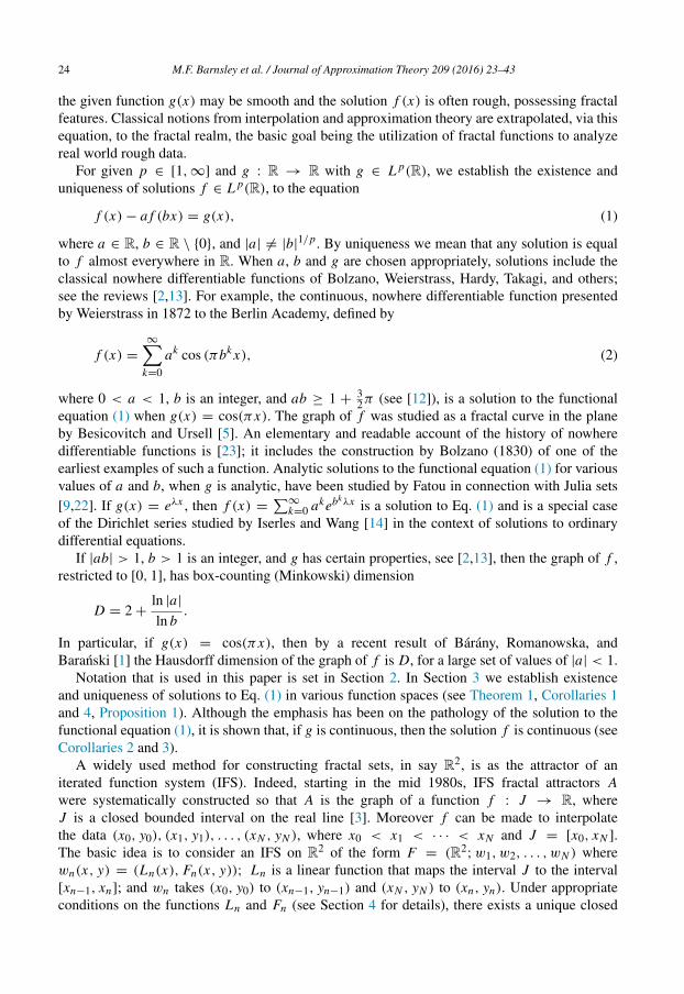
Fig. 1. This illustrates how the graph of a fractal interpolation function is made of affinely transformed copies of itself,and how it interpolates the data. The four large dots represent the data and the parallelograms are affine transforms of arectangle that contains the graph and has sides parallel to the axes.

bounded nonempty set A ⊂ R2 that obeys the self-referential equation A = ∪Nn=1 wn(A), which

says A is made of transformed copies of itself, for example as illustrated in Fig. 1. This set A iscalled the attractor of the IFS, and has the property that it is the graph of a continuous function,defined on J , that interpolates the data.

The book [18] is a reference on such fractal interpolation functions constructed via an IFS.One of the appeals of the theory is that it is possible to control the box-counting dimension andsmoothness of the graph of the interpolant. The solutions to the functional equation (1) include,not only the classical nowhere differentiable functions, but also fractal interpolation functions.This is the subject of Section 4, in particular Theorems 2 and 3. One impetus for the researchreported here is the work on fractal interpolation by Massopust [18], Navascues [21,19,20], andChand and his students [6].

In Section 5, Eq. (1) and the theory surrounding it are leveraged to obtain orthogonalexpansions – that we call Weierstrass Fourier series – and corresponding approximants, forvarious functions, both smooth and rough, using approximants with specified Minkowski andeven Hausdorff dimension.

Some ideas in the present work are anticipated, at least in flavor, in Deliu and Wingren [7]and Kigami and his collaborators [16,25]. But, as far as we know, our main observations, namelyTheorem 1 and its corollaries, Theorems 2 and 3, and Theorem 4, are new.

2. Notation

For p ∈ [1, ∞), L p(X) denotes the Banach space of functions f : X → R such thatX

| f (x)|pdx < ∞,

where the integration is with respect to Lebesgue measure on X . In this paper, X will be R, aclosed interval of R, or an interval of the form [c, ∞), (−∞, c] or (−∞, c]∪ [c′, ∞). The spaceL∞(X) denotes the Banach space of functions f : X → R such that the essential supremum of


| f | is bounded. For all p ∈ [0, ∞], the norm of f ∈ L p(X) is denoted ∥ f ∥p, where

∥ f ∥p =

X

| f (x)|pdx

1/p

when p ∈ [1, ∞),

∥ f ∥∞ = inf{M ∈ [0, ∞) : | f (x)| ≤ M for almost all x ∈ X}.

The norm of a bounded linear operator H : L p(X) → L p(X) is defined by

∥H∥p = max{∥H f ∥p : ∥ f ∥p = 1}.

The space of bounded uniformly continuous real valued functions with the supremum norm isdenoted CB(X). Further let

CkB(X) = { f : f ( j)

∈ CB(X), j = 0, 1, . . . , k}.

For a bounded continuous function f and α ∈ (0, 1], let

[ f ]α = supx,y∈X, x=y

| f (x) − f (y)|

|x − y|α.

For k ∈ N ∪ {0}, the Holder space

Ck,αB (R) := { f ∈ CB(R) : f ( j)

∈ CB(R), j = 0, 1, .., k, ∥ f ∥Ck,α < ∞}

where

∥ f ∥Ck,α :=

kj=0

∥ f ( j)∥∞ + [ f (k)

]α

is a Banach space.Let k ≥ 1 be an integer and f ∈ L1

loc(R), the space of all locally integrable functions. Afunction g ∈ L1

loc(R) is a weak-derivative of f of order k ifR

g(x)φ(x)dx = (−1)k

Rf (x)φ(k)(x)dx

for all φ ∈ C∞c (R), where C∞

c (R) is the space of continuous functions with compact support,having continuous derivatives of every order.

For 1 ≤ p ≤ ∞ and k ∈ N ∪ {0}, let W k,p(R) denote the usual Sobolev space. That is,

f ∈ W k,p(R) ⇐⇒ f ( j)∈ L p(R), j = 0, 1, . . . , k,

where f ( j) denotes the j th weak or distributional derivative of f . The space W k,p(R) endowedwith the norm

∥ f ∥W k,p :=

f (k)

p+ ∥ f ∥p

is a Banach space.Consider the difference operator

∆h f (x) = f (x − h) − f (x)

and define the modulus of continuity by

ω2p( f, t) = sup

|h|≤t∥∆2

h f ∥p.


For n ∈ N ∪ {0}, s = n + α, 0 < α ≤ 1 and 1 ≤ p, q ≤ ∞, the Besov space Bsp,q(R) consists

of all functions f such that

f ∈ W n,p(R),

∞

0

w2p( f (n), t)

tα

q dt

t< ∞.

The functional

∥ f ∥Bsp,q

:=

∥ f ∥

qW n,p +

∞

0

w2p( f (n), t)

tα

q dt

t

1q

is a norm which turns Bsp,q(R) into a Banach space.

3. Solutions of the functional equation

The functional equation (1) can be expressed as

Ma,b f = g, (3)

where the linear operator Ma,b is defined as follows.

Definition 1. For all p ∈ [1, ∞], a, b ∈ R, b = 0, the linear operators Tb : L p(R) → L p(R)

and Ma,b : L p(R) → L p(R) are given by

(Tb f )(x) = f (bx)

Ma,b f = (I − aTb) f

for all x ∈ R and all f ∈ L p(R). By convention, if p = ∞ and b = 0, then |b|1p = 1.

It is easy to check that Eq. (3) is equivalent to

M 1a , 1

bf = g, (4)

where g = −1a T1

bg. This fact is used in the proof of the following theorem.

Theorem 1. For all p ∈ [1, ∞], a, b ∈ R, b = 0, and |a| = |b|1p , the linear operators T = Tb

and M = Ma,b are homeomorphisms from L p(R) to itself. In particular,

1.

T −1b = T1

b

2.

∥Tb∥p = |b|−

1p

3. 1 −|a|

|b|1p

∥ f ∥p ≤Ma,b f

p ≤

1 +

|a|

|b|1p

∥ f ∥p


4.

Ma,b−1

=

∞n=0

an Tbn if |a| < |b|

1p ,

−

∞n=1

1a

n

T1b

n if |a| > |b|1p .

Proof. It is readily verified that T is invertible with inverse T −1b = T1

band that the formula (2)

for the p-norm of Tb holds. ConsequentlyT −1b

p

= |b|1p .

Inequality (3) follows from (2) and the triangle inequality.

Assume that |a| < |b|1p . To show that M is injective in this case, assume that M f = 0, i.e.,

∥ f − aTb f ∥p = 0. Then

0 = ∥ f − aTb f ∥p ≥ ∥ f ∥p − |a| ∥Tb∥p ∥ f ∥p = (1 − |a| ∥Tb∥p) ∥ f ∥p

=

1 − |a| |b|

−1p

∥ f ∥p ≥ 0,

which implies that ∥ f ∥p = 0. To show that M is surjective and that a solution to M f = g inL p(R) is

f =

∞n=0

anTbn g

first note that the series is absolutely and uniformly convergent in L p(R). This is because thepartial sums are Cauchy sequences. Now, using the continuity of M : L p(R) → L p(R) andequality (2) in the statement of the theorem, we have

M

∞

n=0

anTbn g

= lim

k→∞

k

n=0

an MTbn g

= lim

k→∞(I − ak+1Tb

k+1)g = g.

Now assume that |a| > |b|1p . By the paragraph above M 1

a , 1b

is injective. But it is easilychecked, using statement (2) in the theorem, that Ma,b f = 0 if and only if M 1

a , 1b

f = 0.Therefore Ma,b is injective. To show that M := Ma,b is surjective and that a solution to M f = gin L p(R) is

f = −

∞n=1

1a

n

T1b

ng, (5)

note that, by the paragraph above,

M 1a , 1

b

−1

−1a

T1b

g

=

∞n=0

1a

n

T1b

n

−1a

T1b

g

= −

∞n=1

1a

n

T1b

ng.

Referring to Eq. (4), this verifies Eq. (5). �


The next corollary on existence and uniqueness of solutions to Eq. (1) follows at once fromTheorem 1.

Corollary 1. Assume that a, b ∈ R, b = 0, and |a| = |b|1p . For any g ∈ L p(R), p ∈ [1, ∞],

there is a unique solution f ∈ L p(R) to the equation

f (x) − a f (bx) = g(x),

and the solution is given by the following series that are absolutely and uniformly convergent inL p(R):

f (x) =

∞n=0

an g(bn x) if |a| < |b|1p

−

∞n=1

1a

n

g x

bn

if |a| > |b|

1p .

(6)

Remark 1. Recall that the adjoint of a bounded linear operator A : X → Y is the operatorA∗

: Y ∗→ X∗ defined by (A∗µ)(x) = µ(Ax) for all µ ∈ Y ∗ and x ∈ X , where X∗ denotes the

dual space of X . For 1 ≤ p < ∞ there is a canonical isomorphism between L p(R)∗ and Lq(R),where 1

p +1q = 1. For each linear functional µ ∈ L p(R)∗, this isomorphism associates a unique

representative g ∈ Lq(R) such that µ( f ) =

R f (x)g(x) dx for all f ∈ L p(R). It is routine toshow that

T ∗

b =1b

T1b

in the sense that, if the representative of µ ∈ L p(R)∗ in the space Lq(R) is g, then therepresentative of T ∗

b µ is b−1Tb−1 g. Similarly

M∗

a,b = M ab , 1

b.

Remark 2. If b = 0, then Eq. (1) has solution

f (x) = g(x) +a

1 − ag(0).

So, for all a = 1, there is a well-defined solution f (x) for all x ∈ R, for each specified value ofg(0). Since, as a element of L p(R), the function g is defined only up to a set of measure 0, thevalue g(0) has little meaning. Thus it does not make sense to consider Eq. (1) in L p(R) whenb = 0. However, the problem of finding f for a given g is well-posed in spaces such as CB(R),even when b = 0.

In view of Remark 2, except where otherwise stated, it is assumed throughout this paper that

b = 0 and |a| = |b|1p . The results in Theorem 1 and its Corollary 1 hold for various spaces

related to the L p-spaces. Corollaries 2, 3, and 4 concern these related spaces.

Corollary 2. Assume that a, b ∈ R, b = 0, and |a| = 1. For any g ∈ CB(R), there is a uniquesolution f ∈ CB(R) to the equation

f (x) − a f (bx) = g(x),


and the solution is given by the following series that are absolutely and uniformly convergent:

f (x) =

∞n=0

an g(bn x) if |a| < 1

−

∞n=1

1a

n

g x

bn

if |a| > 1.

Proof. If |a| < 1, then∞

n=M an g(bn x) <

|a|M

1−|a|∥g∥∞. Therefore

limM→∞

supx∈R

∞n=M

an g(bn x)

= 0,

which implies

∞

n=0 an g(bn x) is absolutely and uniformly convergent. Since g ∈ CB(R), itfollows that the infinite sum is a continuous function. That the series is a solution of the functionalequation can be verified at once by substitution, see also Corollary 1. A similar argument appliesin the case |a| > 1. �

The following relationships between the continuity of f and the continuity of g follow as inCorollary 2.

Corollary 3. For the equation Ma,b f = g in L∞(R), if |a| < 1, then the following hold.

1. If b > 0, then f ∈ CB([0, ∞)) if and only if g ∈ CB([0, ∞)).2. If b ≥ 1, then f ∈ CB([1, ∞)) if and only if g ∈ CB([1, ∞)).3. If 0 < b ≤ 1, then f ∈ CB([0, 1]) if and only if g ∈ CB([0, 1]).

A similar set of statements hold when CB(X) is replaced by C ′

B(X), the set of functions inCB(X) with countably many discontinuities.

Remark 3. If, in Corollary 2, g ∈ L∞(R) is assumed piecewise continuous with countablymany points of discontinuity, rather than continuous, then it follows by a similar argument thatthe solution f ∈ L∞(R) to M f = g is piecewise continuous with at most countably many pointsof discontinuity.

Remark 4. Examples related to fractal interpolation (see Example 1) show that f = M−1g maybe continuous on [0, 1] even if g possesses discontinuities.

Unlike continuity, it is well-known from basic real analysis that f = M−1a,bg may fail to be

differentiable even if g is differentiable. Vice versa, when |a| > 1 and g is continuous, f maybe more differentiable than g. Thus, in a general sense, for |a| < 1, the mapping M−1

a,b is a“roughing” operation, and for |a| > 1, it is a “smoothing” operation.

The following estimate is worth mentioning.

Proposition 1. Consider the equation Ma,b f = g for f ∈ CB([0, ∞)), |a| < 1 and b > 0.Then the uniform distance between f and g satisfies

∥g − f ∥∞ = ∥g − M−1a,bg∥∞ ≤

|a|

1 − |a|∥g∥∞.


Consequently

∥I − M−1a,b∥∞ ≤

|a|

1 − |a|.

Proof. Note thatg(x) − M−1a,bg(x)

=g(x) −

∞n=0

ang(bn x)

≤

∞n=1

|a|n∥g∥∞

=|a|

1 − |a|∥g∥∞.

Therefore ∥g − f ∥∞ ≤|a|

1−|a|∥g∥∞, proving the assertion. �

The term automorphism in the next corollary refers to a linear map that is a homeomorphismof a space to itself. In particular, statement (6) in the corollary is used in Section 5.

Corollary 4. If M = Ma,b is the operator of Definition 1, with |a| = |b|1p , then M is an

automorphism when considered as a mapping on

1. L p([0, ∞)) or L p((−∞, 0]) if b > 0;2. L p([1, ∞)) or L p((−∞, −1]) if b > 1;3. L p((−∞, −1] ∪ [1, ∞)) if |b| > 1;4. L p([0, 1]) or L p([−1, 0]) if 0 < b < 1;5. L p([−1, 1]) if 0 < |b| ≤ 1;6. L∞([0, ∞)) ∩ P if b ∈ N, |a| < 1, where P is the set of functions f : [0, ∞) → R

such that f (x) = f (x + 1) for all x ∈ (0, ∞). This is with the understanding that, forg ∈ L∞([0, ∞)) ∩ P , a representative of M−1g can be chosen to lie in P .

Proof. (1) The space L p(R) is the direct sum of two subspaces L+ and L−, the first consistingof functions which vanish over the negative reals and the second consisting of functions whichvanish over the positive reals. Since each of these two subspaces is mapped into itself by M andsince M is bijective on L p(R), it follows that M restricted to L+ and M restricted to L− are bothbijective. The proofs of (2)–(6) are similar, some using Corollary 1. �

For appropriate values of a and b, the operator Ma,b also defines an automorphism insome standard spaces of smooth functions that occur frequently in various fields of analysissuch as approximation theory, numerical analysis, functional analysis, harmonic analysis, andin particular in connection with partial differential equations. The proof is similar to that ofTheorem 1, and hence is omitted.

Proposition 2. For the operator Ma,b specified in Definition 1 the following properties hold.

1. If |a| < min|b|

1p , |b|

1p −k or |a| > max

|b|

1p , |b|

1p −k, then Ma,b is an automorphism on

Sobolev space W k,p(R).2. If |a| < min

1, |b|

−1, |b|−2, . . . , |b|

−k, |b|−α

or |a| > max1, |b|

−1, |b|−2, . . . , |b|

−k,

|b|−α, then Ma,b is an automorphism on Holder space Ck,α

B (R).

3. If |a| < min|b|

1p , |b|

1p −n

, |b|1p −n−α or |a| > max

|b|

1p , |b|

1p −n

, |b|1p −n−α, then Ma,b is

an automorphism on Besov space Bsp,q(R).


In all the above cases Ma,b−1

=

∞

n=0 an T nb for the first set of admissible values of

parameters a, b and Ma,b−1

= −

∞

n=1

1a

nT n

1b

for the second set of admissible values of

parameters a, b.

Remark 5. A straightforward but useful consequence of the fact that M−1a,b is an automorphism

on various spaces is the following. It is well known that Schauder bases are preserved underan isomorphism. Consequently, if { fn}

∞

n=1 is a Schauder basis for X , where X is one of the

spaces L p(R), W k,p(R), Ck,αB (R) or Bs

p,q(R), then {M−1a,b fn}

∞

n=1 is a Schauder basis consistingof rough analogues of the functions { fn}

∞

n=1. In particular, if { fn}∞

n=1 is an orthonormal basis forthe Hilbert space L2(R) or W k,2(R), then {M−1

a,b fn}∞

n=1 is a Riesz basis for L2(R) or W k,2(R).

Some orthonormal bases consisting of rough functions obtained via M−1a,b are discussed in detail

in Section 5.

4. Fractal Interpolation

To illustrate how standard fractal interpolation theory fits into the functional equationframework, consider a given set of data points {(xn, yn)}N

n=0 ⊂ R2, N > 1, with 0 = x0 <

x1 < x2 · · · < xN = 1. At minimum what one seeks is a function f : [0, 1] → R, such that

1. f interpolates the data, i.e., f (xn) = yn, n = 0, 1, . . . , N ;2. there is an IFS F = (R2

; w1, w2, . . . , wN ) whose attractor is the graph of the function f onthe interval [0, 1];

3. parameters of the IFS can be varied to control continuity and differentiability of f and theMinkowski dimension of the graph of f .

The IFS maps wn, n = 1, 2, . . . , N , that are studied extensively in fractal interpolationtheory [3] are of the form

wn(x, y) =Ln(x), Fn(x, y)

, (7)

where

Ln(x) = an x + bn, Fn(x, y) = αn y + gn(x), (8)

|αn| < 1; gn : [0, 1] → R is continuous; and

Ln(x0) = xn−1,

Ln(xN ) = xn,

Fn(x0, y0) = yn−1,

Fn(xN , yN ) = yn,(9)

for all n = 1, 2, . . . , N . In this case there is a unique attractor of F , and it is the graph of acontinuous function f that interpolates the data [3]. The parameters αn and gn can be varied tocontrol continuity and differentiability of f and the Minkowski dimension of the graph of f .

We specialize to the uniform partition of [0, 1] and a constant scaling factor, i.e.,

Ln(x) =x + n − 1

N, αn = a, |a| < 1, (10)

for all n = 1, 2, . . . , N .The next two theorems make precise the close relationship between fractal interpolation

functions and solutions to the “Weierstrass-type” functional equation.


Theorem 2. Given data points {(xn, yn)}Nn=0 ⊂ R2, N > 1, let F be the IFS defined by

Eqs. (7)–(10), and let f be the function on [0, 1] whose graph is the attractor of F and thatinterpolates the data.

Then f is the unique solution to the functional equation f (x) − a f (N x) = g(x) consideredin the space L∞([0, ∞)) ∩ P of Corollary 4, where

g(x) =

gn(L−1n (x)) if x ∈ [xn−1, xn), n = 1, 2, . . . , N ,

gN (1) if x = 1,

g(x − 1) if x ∈ (1, ∞).

Proof. It follows immediately from the fact that the graph of f (x) is the attractor of the IFS withfunctions as in Eq. (7) that

{(x, f (x)) : x ∈ [0, 1]} =

Nn=1

{(Ln(x)), a f (x) + gn(x) : x ∈ [0, 1]}

=

Nn=1

(x, a f (L−1

n (x))) + gn(L−1n (x)) : x ∈

n − 1

N,

n

N

.

This implies, for x ∈ [(n −1)/N , n/N ], n = 1, 2, . . . , N and in the space L∞([0, ∞))∩ P , that

f (x) = a f (N x − (n − 1)) + gn(L−1n (x)) = a f (N x) + g(x). �

Theorem 3. Let f be the unique solution to the functional equation f (x) − a f (N x) = g(x)

considered in the space L∞([0, ∞))∩P , where g ∈ L∞([0, ∞))∩P has the following properties

1. g is continuous on the intervals [x0, x1], (x1, x2], . . . , (xN−1, xN ],2. the limit from the right g( n

N +) exists for n = 1, . . . , N − 1.

Then f interpolates the data {(xn, yn), n = 0, 1, 2, . . . , N }, where xn = n/N and

y0 = g(0)/(1 − a)

yN = g(1)/(1 − a)

yn = g(xn) +a

1 − ag(1), n = 1, 2, . . . , N − 1.

Moreover, the closure of the graph of f restricted to the domain [0, 1] is the unique attractorof the IFS W = ([0, 1] × R; w1, w2, . . . , wN ), where wn(x, y) = (Ln(x), ay + gn(x)), n =

1, 2, . . . , N, and

Ln(x) = (x + n − 1)/N

gn(x) =

gLn(x)

if 0 < x < 1

g

n − 1

N+

if x = 0

g n

N

if x = 1.

If, in addition to properties (1–2) of the function g, we have

(3) g n

N+

− g

n

N

=

a

1 − a(g(1) − g(0))

for n = 1, 2, . . . , N − 1, then f is continuous on [0, 1], and the graph of f restricted to thedomain [0, 1] is the unique attractor of the IFS W.


Proof. Concerning the interpolation of the data, assume that |a| < 1. Statement (1) ofCorollary 4 guarantees a unique solution given by f (x) =

∞

k=0 ak g(N k x). Substituting x = 0into the functional equation, we obtain f (0) − a f (0) = g(0) which implies f (0) =

g(0)1−a = y0.

Substituting x = 1 in the series expansion yields

f (1) =

∞k=0

ak g(N k) =

∞k=0

ak g(1) = yN .

With 1 ≤ n ≤ N − 1, substituting x = xn and using properties of g, we have

f (xn) =

∞k=0

ak g(N k xn) =

∞k=0

ak g

N k n

N

= g

n

N

+

∞k=1

ak g(N k−1n)

= g n

N

+

∞k=1

ak g(1) = g(xn) + ayN = yn .

Concerning the statement about the closure of the graph of f , we consider the followingset-valued map associated with the IFS W . With a slight abuse of notation, we shall denote theassociated map also by W and let W : 2[0,1]×R

→ 2[0,1]×R defined by

W (B) =

Ni=1

wi (B).

Let G := {(x, f (x)) : x ∈ [0, 1]}. It is well known, see for example [4, Theorem 3.2], that underthe stated conditions the IFS W possesses a unique attractor. The attractor is the unique compactset A ⊂ [0, 1] × R such that W (A) = A. It suffices to show that W (G) = G. Note that f isperiodic with period 1.

To show that W (G) = G, we first show that

W (G) ⊆ G, (11)

where G = G \{(0, f (0)), (1, f (1))}. For any n = 1, 2, . . . , N , let (x ′, y′) ∈ wn(G), Then thereis an (x, y) such that x ∈ (0, 1], y = f (x), x ′

= Ln(x) = (n − 1 + x)/N , and

y′= ay + gn(x) = a f (x) + g(Ln(x)) = a f (N x ′

− n + 1) + g(Ln(L−1n (x ′)))

= a f (N x ′) + g(x ′).

This implies that y′= f (x ′), so that (x ′, y′) ∈ G.

We next show thatG ⊆ W (G), (12)

where G = G \ {(n/N , f (n/N )), n = 0, 1, 2, . . . , N }. Assume that (x, y) ∈ G and, withoutloss of generality, that x ∈ ((n − 1)/N , n/N ). Let x ′

= L−1n (x), y′

= f (x ′). Then

y = f (x) = a f (N x) + g(x) = a f (x ′+ N − 1) + g(Ln(x ′)) = a f (x ′) + gn(x ′).

Therefore (x, y) = wn(x ′, y′) ∈ W (G).Note that the map wn : [0, 1] × R → ((n − 1)/n, n/N ] × R is a homeomorphism. From

Eqs. (11) and (12), respectively,

W (G) = W (G) = W (G) ⊆ G

G = G ⊆ W (G) = W (G).


With the additional assumption (3) we have, F1(x0, y0) = y0 and for n = 2, 3, . . . , N

Fn(x0, y0) = ay0 + gn(0)

= ay0 + g

n − 1

N+

= ay0 + g

n − 1

N

+

a

1 − a(g(1) − g(0))

= yn−1.

Similarly Fn(xN , yN ) = yn . Therefore the functions Fn satisfy Eq. (9), in which case the attractorof the IFS is the graph of a continuous function. �

The present formalism allows both continuous and discontinuous interpolants, as illustrated inExample 1, in contrast to continuous interpolants in the traditional theory of fractal interpolationfunctions. Furthermore, the fractal interpolation functions obtained herein can be evaluatedpointwise to desired precision, by summing absolutely and uniformly convergent series. We notethat discontinuous fractal functions are also mentioned in [20].

Example 1. It follows from Theorems 2 and 3 that the attractor A ⊂ [0, 1] × [−1, 1] of thecontractive IFS

W = {R2; w1(x, y) = (x/2, ay), w2(x, y) = (x/2 + 1/2, (1 − a) + ay)},

where −1 < a < 1, is the closure of the graph, restricted to the domain [0, 1], of the uniquefunction f in the space L∞([0, ∞)) ∩ P that is the solution to the equation

f (x) − a f (2x) = g(x),

where

g(x) =

0 for x ∈ [0, 1/2]

1 − a for x ∈ (1/2, 1]

g(x − n) for x ∈ (n, n + 1], n ∈ N.

Moreover, the function f interpolates the data {(0, 0), (0.5, a), (1, 1)}. The function g :

[0, ∞) → R is not continuous on [0, 1]. The function f : [0, 1] → R, that can be representedby the uniformly and absolutely convergent series

f (x) =

∞k=0

ak g(2k x),

is not continuous for a = 1/2. That the function f is discontinuous on [0, 1] for a = 1/2 can beverified, for instance, by showing that f (1/2+) = f (1/2) and f (0+) = f (0) cannot be satisfiedsimultaneously. When a = 1/2, the function f is continuous; in fact f (x) = x .

For a formulation more closely related to continuous fractal interpolation functions, asillustrated in the next paragraph, let f0, g0 ∈ L∞([0, ∞)) ∩ P be such that f0(x) is continuousfor x ∈ [0, 1] (from the right at x = 0 and from the left at x = 1) with

f0(0) = y0f0(1) = yNf0(x) = f0(x − 1) for x ∈ (1, ∞),


and g0 : [0, ∞) → R is continuous and such that

g0(0) = g0(1) = 0g0(x) = g0(x + 1) for all x ∈ [0, ∞)

g0(xn) = yn − f0(xn) for n = 1, 2, . . . , N − 1.

Then it is readily confirmed that

g(x) := g0(x) + f0(x) − a f0(N x) (13)

satisfies the conditions (1), (2), (3) of Theorem 3. In particular, the solution to the functionalequation f (x) − a f (N x) = g(x) is continuous on [0, 1] and passes through the data. Thatis, the solution f (x) is a continuous fractal interpolation function on the interval [0, 1]. Note,however, that typically g(x) is not continuous for x ∈ (0, 1) even though g0(x) is continuous forall x ∈ [0, ∞) and f0(x) is continuous for x ∈ (0, 1).

In this setting, the free parameters, namely the “base function” f0, the function g0, and thevertical scaling parameter a, may be chosen to obtain diverse fractal interpolation systems, forinstance, Hermite and spline fractal interpolation functions [3,6,21]. They can also be chosen tocontrol the Minkowski dimension and other properties of the graph of the approximant f . Forexample, it is reported in [2] that both the Minkowski dimension and the packing dimension ofthe graph of f are given by D = max{2 +

ln|a|

ln N , 1}, for various classes of function g0. Consistentformulas for the Minkowski dimensions related to graphs of a fractal interpolation function areestablished in [8,10,11].

In Refs. [3,19] it is observed that the notion of fractal interpolation can be used to associate anentire family of fractal functions {hα

: α ∈ (−1, 1)N} with a prescribed continuous function h

on a compact interval. To this end, one may consider Eq. (8) with gn(x) = hLn(x)

− αnq(x),

where q : [0, 1] → R is a continuous function such that q ≡ h and q interpolates h at theextremes of the interval [0, 1]. Each function hα in this family is referred to as α-fractal functionor “fractal perturbation” corresponding to h. In our present setting, the function f is the fractalperturbation corresponding to g0 + f0 with base function f0 and constant scale vector α whosecomponents are a. Therefore, the α-fractal function and the approximation classes obtainedthrough the corresponding fractal operator (see, for instance, [19,24]) can also be discussed usingthe present formalism.

5. Weierstrass Fourier approximation

This section deals with a framework for a “fractal” Fourier analysis. A natural completeorthonormal basis set of fractal functions is provided that serves as a rough analog of the standardsine–cosine Fourier basis. These fractal counterparts are obtained as solutions f to the functionalequation (1), with g ∈ {sin 2kπx, cos 2kπx}

∞

k=1 ∪ {1}.

Proposition 3. Let f (x) be the solution to f (x) − a f (bx) = g(x) in L2(R) where |a| < |b|1/2.

If {gk}∞

k=1 is an orthononormal basis for L2(R), then

⟨ fk, fl⟩ = c +

∞n=1

a2n

bn

nm=1

bm

am ⟨gk, (Tbm + T ∗

bm )gl⟩,

where c = (1 − a2/b)−1.


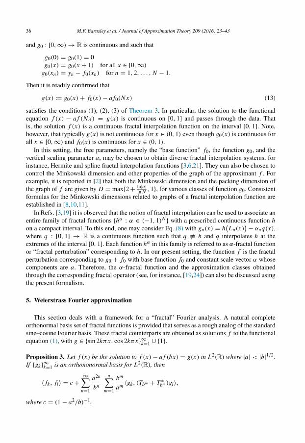
Proof. Define Ta,b = aTb. We have T ∗

a,b = Tab , 1

b, and also Ta,bTc,d = Tac,bd = Tc,d Ta,b. On

taking the product, term-by-term, of two absolutely and uniformly convergent series of linearoperators, we obtain

((I − Ta,b)∗(I − Ta,b))

−1= (I − Ta,b)

−1(I − T ∗

a,b)−1

= (I − Ta,b)−1

I − Tab , 1

b

−1

=

∞

n=0

anT nb

∞

m=0

a

b

mT m

1b

=

∞n=0

∞m=0

an+m

bm T nb T m

1b

=

∞n=0

∞m=0

an+m

bm Tbn−m .

Now let {gk}∞

k=1 be an orthononormal basis for L2(R). Let fk = M−1a,b(gk) = (I − Ta,b)

−1gk .Since, by Theorem 1, (I − Ta,b)

−1 is a linear homeomorphism on L2(R), the set of functions{ fk}

∞

k=1 is a Riesz basis for L2(R). Then

⟨ fk, fl⟩ = ⟨gk, ((I − Ta,b)∗(I − Ta,b))

−1gl⟩

=

∞n=0

∞m=0

an+m

bm ⟨gk, Tbn−m gl⟩

=

∞n=0

a2

b

n

+

∞n,m=0m<n

an+m

bm ⟨gk, Tbn−m gl⟩ +

∞n,m=0m>n

an+m

bm ⟨gk, Tbn−m gl⟩

= c +

∞n,m=0m<n

an+m


∞n,m=0m<n

an+m

bn ⟨gk, Tbm−n gl⟩

= c +

∞n,m=0m<n

an+m


∞n,m=0m<n

an+m

bm ⟨gk, T ∗

bn−m gl⟩

= c +

∞n=1

n−1m=0

an+m

bm ⟨gk, (Tbn−m + T ∗

bn−m )gl⟩

= c +

∞n=1

nm=1

a2n−m

bn−m ⟨gk, (Tbm + T ∗

bm )gl⟩

= c +

∞n=1

a2n

bn

nm=1

bm

am ⟨gk, (Tbm + T ∗

bm )gl⟩

where c = (1 − a2/b)−1. �

A similar looking but different expression can be obtained in the case |a| > |b|1/2. Clearly,

such series are amenable to computation, as we illustrate in the next section. For another example,

the gk in Proposition 3 could be (√

π2kk!)−12 Hk(x) exp(−x2/2), where the Hk are Hermite

polynomials [15].


5.1. Weierstrass Fourier basis

Working in L2([0, 1]), the inner product is ⟨ f, h⟩ := 1

0 f (x)h(x)dx . The set of functions{√

2 cos k2πx}∞

k=1 ∪ {√

2 sin k2πx}∞

k=1 ∪ {1} is a complete orthonormal basis for L2([0, 1]).Consider these as functions on R, periodic of period 1. Let

ck(x) =√

2 cos k2πx,

sk(x) =√

2 sin k2πx,

e(x) = 1,

for all k ∈ N and x ∈ R. Inner products are given by

⟨sk, sl⟩ = ⟨ck, cl⟩ = δk,l ,

⟨sk, cl⟩ = ⟨e, ck⟩ = ⟨e, sk⟩ = 0, ⟨e, e⟩ = 1,

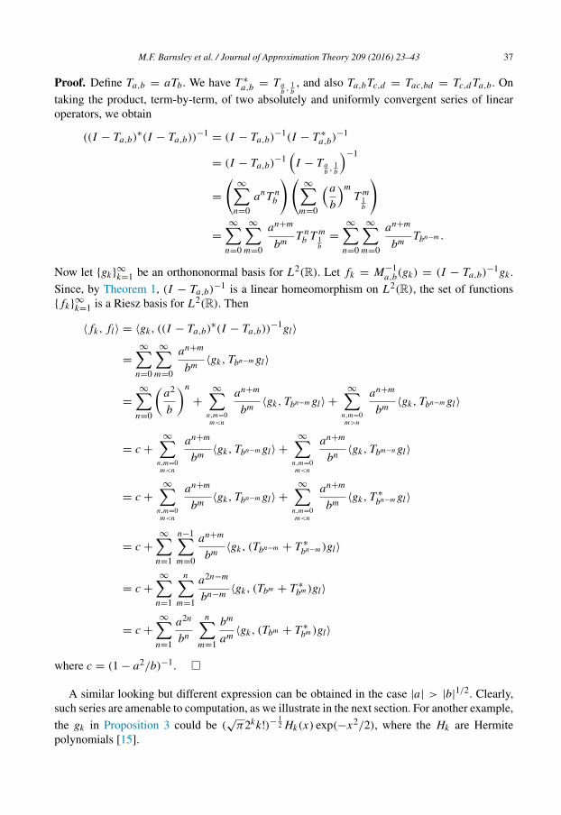
for all k, l ∈ N.Let b = 2, |a| < 1, and M = Ma,b. In view of statement (6) of Corollary 4, and the fact that

the restriction to [0, 1] of functions in L∞([0, ∞))∩ P can be endowed with the L2 norm, a newnormalized basis for L2([0, 1]) is {e,ck,sk : k ∈ N}, where

e = (1 − a) M−1(e) = eck =

1 − a2 M−1(ck)sk =

1 − a2 M−1(sk).

For 1 ≤ k ≤ l, the inner products are

⟨ck,cl⟩ = 2(1 − a2)

∞n,m=0

an+m 1

0(cos kπ2n+1x)(cos lπ2m+1x)dx

= (1 − a2)

∞n,m=0

an+mδ2nk,2m l = (1 − a2)

∞n,m=0n≥m

an+mδ2nk,2m l

= (1 − a2)

∞n,m=0n≥m

an+mδ2n−m k,l = (1 − a2)

i,m≥0

a2m+iδ2i k,l

=

a j if l = 2 j k,

0 otherwise.

Similar expressions are obtained for {sk}∞

k=1. In summary, for all k, l ∈ N,

⟨ck,e⟩ = ⟨sk,e⟩ = ⟨ck,sl⟩ = 0 and ⟨e,e⟩ = 1,

⟨ck,cl⟩ = ⟨sk,sl⟩ =

a j if k = 2 j l or l = 2 j k for some j ∈ N ∪ {0},

0 if k = 2 j l and l = 2 j k for all j ∈ N ∪ {0}.

(14)

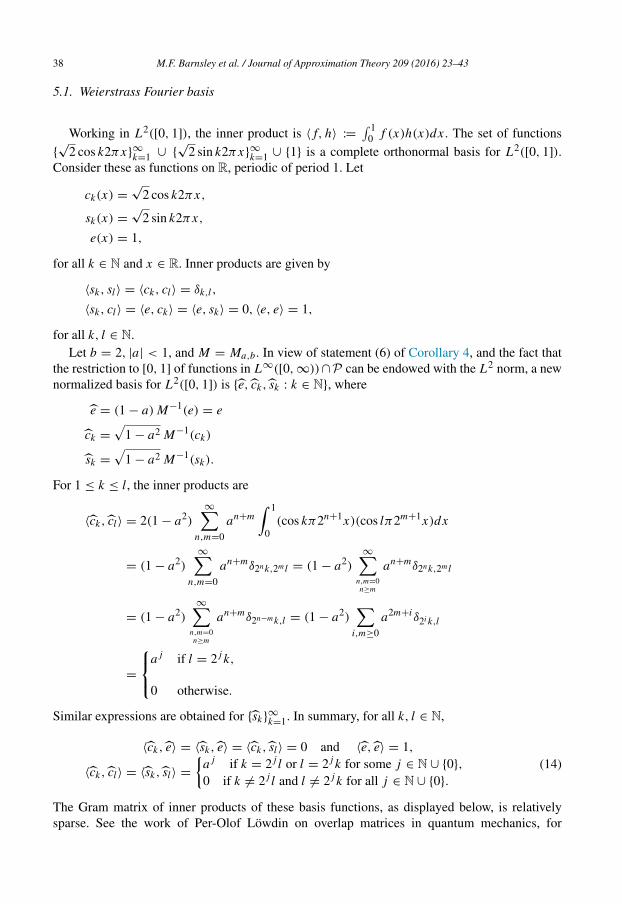
The Gram matrix of inner products of these basis functions, as displayed below, is relativelysparse. See the work of Per-Olof Lowdin on overlap matrices in quantum mechanics, for


example [17].

(⟨sk,sl⟩)∞

k,l=1 = (⟨ck,cl⟩)∞

k,l=1 =

1 a1 0 a2 0 0 0 a3 .

a1 1 0 a1 0 0 0 a2 .

0 0 1 0 0 a1 0 0 .

a2 a1 0 1 0 0 0 a1 .

0 0 0 0 1 0 0 0 .

0 0 a1 0 0 1 0 0 .

0 0 0 0 0 0 1 0 .

a3 a2 0 a1 0 0 0 1 .

. . . . . . . . .

.

Note that, for m = 0, 1, 2, 3,

det (⟨ck,cl⟩)2m

k,l=1 = (1 − a2)2m,

which suggests that this formula holds for all m ∈ N ∪ {0}.The graph of each functionck,sk has Minkowski (and in “many cases” Hausdorff) dimension

D = 2 + (ln a) / ln 2 when a > 0.5; see [1,13]. It is straightforward to apply the Gram–Schmidtalgorithm to obtain the complete orthonormal basis of Weierstrass nowhere differentiablefunctions given in the following theorem.

Theorem 4. The set of functions {1,ck,sk : k ∈ N}, where

ci =

ci if i is oddci − aci/2√

1 − a2=

1 − a2 ci − a ci/2 if i is even

si =

si if i is oddsi − asi/2√

1 − a2=

1 − a2si − a si/2 if i is even,

is a complete orthonormal basis for L2([0, 1]).

Proof. Using the relations in Eq. (14) it follows readily that, if k is odd and l is even, then⟨ck,cl⟩ = 0 unless l = k2 j for some positive integer j , in which case,

1 − a2 ⟨ck,cl⟩ = ⟨ck,cl⟩ − a ⟨ck,cl/2⟩ = a j− a a j−1

= 0.

For k < l, both even, it again readily follows that ⟨ck,cl⟩ = 0 unless l = k2 j for some positiveinteger j , in which case,

(1 − a2) ⟨ck,cl⟩ = ⟨ck,cl⟩ + a2⟨ck/2,cl/2⟩ − a ⟨ck,cl/2⟩ − a ⟨ck/2,cl⟩

= a j+ a j+2

− a a j−1− a a j+1

= 0.

For k = l, both even,

(1 − a2) ⟨ck,ck⟩ = ⟨ck,ck⟩ + a2⟨ck/2,ck/2⟩ − 2a ⟨ck,ck/2⟩ = 1 + a2

− 2a a = 1 − a2.

To show the equality of the two expressions in the even cases, expressci (orsi ) as a sum ofthe ci ’s (or si ’s) using Eq. (6) and simplify. �


A given function h ∈ L2([0, 1]) has a Fourier expansion in terms of the complete orthonormalbasis {1, sk, ck : k ∈ N}. If h is, in addition, bounded and extended periodically, it has anexpansion, that we refer to as a Weierstrass Fourier series, in terms of the complete orthonormalbasis {1,sk,ck : k ∈ N} of fractal functions.

Theorem 5. If h ∈ L2([0, 1]) has Fourier expansion

h(x) = α0 +

∞n=1

[αn cn(x) + βn sn(x)] ,

then on the interval [0, 1] it also has Weierstrass Fourier expansion

h(x) =α0 +

∞n=1

αncn(x) + βnsn(x),

whereα0 = α0 and

αn =

1 − a2∞

m=0

am αn2m if n is odd

−a αn/2 + (1 − a2)

∞m=0

am αn2m if n is even,

βn =

1 − a2∞

m=0

am βn2m if n is odd

−a βn/2 + (1 − a2)

∞m=0

am βn2m if n is even.

Proof. To computeαn = ⟨h,cn⟩, expresscn andsn in terms of thecn and cn using Theorem 4,then just express in terms of the cn using Eq. (6). The orthogonality relations for the respectivesine and cosine functions yield the formulas in the statement of the theorem, similarly for thecomputation of βn = ⟨h,sn⟩. �

Remark 6. If a = 0, then cn = cn andsn = sn , for all n, and the Weierstrass Fourier seriesreduces to the classical Fourier series.

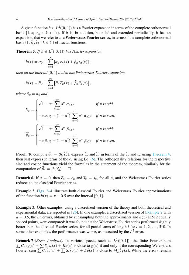
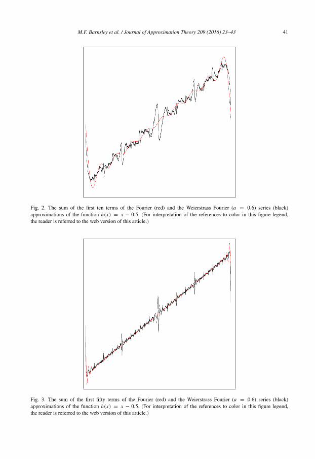
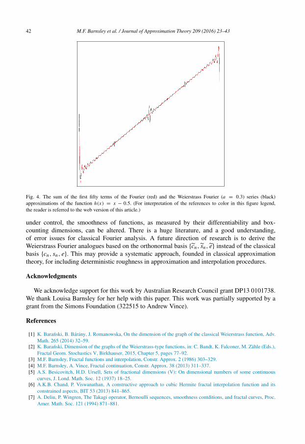
Example 2. Figs. 2–4 illustrate both classical Fourier and Weierstrass Fourier approximationsof the function h(x) = x − 0.5 over the interval [0, 1].

Example 3. Other examples, using a discretized version of the theory and both theoretical andexperimental data, are reported in [26]. In one example, a discretized version of Example 2 witha = 0.5, the L2 errors, obtained by subsampling both the approximants and h(x) at 512 equallyspaced points, were compared: it was found that the Weierstrass Fourier series performed slightlybetter than the classical Fourier series, for all partial sums of length l for l = 1, 2, . . . , 510. Insome other examples, the performance was worse, as measured by the L2 error.

Remark 7 (Error Analysis). In various spaces, such as L2([0, 1]), the finite Fourier sumCncn(x) +

Snsn(x) + Ee(x) is close to g(x) if and only if the corresponding Weierstrass

Fourier sum

Cncn(x) +

Snsn(x) + Ee(x) is close to M−1a,bg(x). While the errors remain


Fig. 2. The sum of the first ten terms of the Fourier (red) and the Weierstrass Fourier (a = 0.6) series (black)approximations of the function h(x) = x − 0.5. (For interpretation of the references to color in this figure legend,the reader is referred to the web version of this article.)

Fig. 3. The sum of the first fifty terms of the Fourier (red) and the Weierstrass Fourier (a = 0.6) series (black)approximations of the function h(x) = x − 0.5. (For interpretation of the references to color in this figure legend,the reader is referred to the web version of this article.)


Fig. 4. The sum of the first fifty terms of the Fourier (red) and the Weierstrass Fourier (a = 0.3) series (black)approximations of the function h(x) = x − 0.5. (For interpretation of the references to color in this figure legend,the reader is referred to the web version of this article.)

under control, the smoothness of functions, as measured by their differentiability and box-counting dimensions, can be altered. There is a huge literature, and a good understanding,of error issues for classical Fourier analysis. A future direction of research is to derive theWeierstrass Fourier analogues based on the orthonormal basis {cn,sn,e} instead of the classicalbasis {cn, sn, e}. This may provide a systematic approach, founded in classical approximationtheory, for including deterministic roughness in approximation and interpolation procedures.

Acknowledgments

We acknowledge support for this work by Australian Research Council grant DP13 0101738.We thank Louisa Barnsley for her help with this paper. This work was partially supported by agrant from the Simons Foundation (322515 to Andrew Vince).

References

[1] K. Baranski, B. Barany, J. Romanowska, On the dimension of the graph of the classical Weierstrass function, Adv.Math. 265 (2014) 32–59.

[2] K. Baranski, Dimension of the graphs of the Weierstrass-type functions, in: C. Bandt, K. Falconer, M. Zahle (Eds.),Fractal Geom. Stochastics V, Birkhauser, 2015, Chapter 5, pages 77–92.

[3] M.F. Barnsley, Fractal functions and interpolation, Constr. Approx. 2 (1986) 303–329.[4] M.F. Barnsley, A. Vince, Fractal continuation, Constr. Approx. 38 (2013) 311–337.[5] A.S. Besicovitch, H.D. Ursell, Sets of fractional dimensions (V): On dimensional numbers of some continuous

curves, J. Lond. Math. Soc. 12 (1937) 18–25.[6] A.K.B. Chand, P. Viswanathan, A constructive approach to cubic Hermite fractal interpolation function and its

constrained aspects, BIT 53 (2013) 841–865.[7] A. Deliu, P. Wingren, The Takagi operator, Bernoulli sequences, smoothness contditions, and fractal curves, Proc.

Amer. Math. Soc. 121 (1994) 871–881.

http://refhub.elsevier.com/S0021-9045(16)30022-3/sbref1








[8] L. Dalla, V. Drakopoulos, M. Prodromou, On the box dimension for a class of nonaffine fractal interpolationfunctions, Anal. Theory Appl. 19 (2003) 220–233.

[9] P. Fatou, Sur les equations fonctionnelles, Bull. Math. France XLVIII (1919) 261.[10] J.S. Geronimo, D.P. Hardin, An exact formula for the measure dimensions associated with a class of piecwise linear

maps, Constr. Approx. 5 (1989) 89–98.[11] D.P. Hardin, P. Massopust, The capacity for a class of fractal functions, Comm. Math. Phys. 105 (1986) 455–460.[12] G.H. Hardy, Weierstrass’s non-differentiable function, Trans. Amer. Math. Soc. 17 (1916) 301–325.[13] B.R. Hunt, The Hausdorff dimension of graphs of Weierstrass functions, Proc. Amer. Math. Soc. 126 (1998)

791–800.[14] A. Iserles, B. Wang, Dirichlet series for dynamical systems of first-order ordinary differential equations, Discrete

Contin. Dyn. Syst. B 19 (2014) 281–298.[15] W. Johnston, The weighted Hermite polynomials form a basis for L2(R), Amer. Math. Monthly 121 (2014)

249–253.[16] J. Kigami, Some functional equations which generate both crinkly broken lines and fractal curves, J. Math. Kyoto

Univ. 27 (1987) 141–149.[17] Per-Olof Lowdine, Linear Algebra for Quantum Theory, Wiley-Interscience, 1998.[18] P. Massopust, Interpolation and Approximation with Splines and Fractals, Oxford University Press, New York,

2010.[19] M.A. Navascues, Fractal polynomial interpolation, Z. Anal. Anwend. 24 (2) (2005) 401–418.[20] M.A. Navascues, Fractal functions of discontinuous approximation, J. Basic Appl. Sci. 10 (2014) 173–176.[21] M.A. Navascues, M.V. Sebastian, Generalization of Hermite functions by fractal interpolation, J. Approx. Theory

131 (1) (2004) 19–29.[22] A.H. Read, The solutions to a functional equation, Proc. Roy. Soc. Edinburgh Ser. A 63 (1952) 336–345.[23] J. Thim, Continuous nowhere differentiable functions (Masters Thesis), Lulea, 2003.[24] P. Viswanathan, A.K.B. Chand, Fractal rational functions and their approximation properties, J. Approx. Theory

185 (2014) 31–50.[25] M. Yamaguti, M. Hata, J. Kigami, Mathematics of fractals, Transl. Math. Monographs 167 (1997) 1–78.[26] S. Zhang, B. Harding, Discrete Weierstrass Fourier transform and experiments, ArXiv:1502.07734v4 [math.NA] 6

Jan 2016.



















http://arxiv.org/1502.07734v4

Documents

Approximation of rough functions