Spline Approximation of Functions and Datafolk.uio.no/in329/nchap5.pdf · 100 CHAPTER 5. SPLINE APPROXIMATION OF FUNCTIONS AND DATA 5.1.2 Cubic Hermite interpolation The piecewise

CHAPTER 5

Spline Approximation of Functionsand Data

This chapter introduces a number of methods for obtaining spline approximations to givenfunctions, or more precisely, to data obtained by sampling a function. In Section 5.1, wefocus on local methods where the approximation at a point x only depends on data valuesnear x. Connecting neighbouring data points with straight lines is one such method wherethe value of the approximation at a point only depends on the two nearest data points.

In order to get smoother approximations, we must use splines of higher degree. Withcubic polynomials we can prescribe, or interpolate, position and first derivatives at twopoints. Therefore, given a set of points with associated function values and first derivatives,we can determine a sequence of cubic polynomials that interpolate the data, joined togetherwith continuous first derivatives. This is the cubic Hermite interpolant of Section 5.1.2.

In Section 5.2 we study global cubic approximation methods where we have to solvea system of equations involving all the data points in order to obtain the approximation.Like the local methods in Section 5.1, these methods interpolate the data, which now onlyare positions. The gain in turning to global methods is that the approximation may havemore continuous derivatives and still be as accurate as the local methods.

The cubic spline interpolant with so called natural end conditions solves an inter-esting extremal problem. Among all functions with a continuous second derivative thatinterpolate a set of data, the natural cubic spline interpolant is the one whose integralof the square of the second derivative is the smallest. This is the foundation for variousinterpretations of splines, and is all discussed in Section 5.2.

Two approximation methods for splines of arbitrary degree are described in Section 5.3.The first method is spline interpolation with B-splines defined on some rather arbitraryknot vector. The disadvantage of using interpolation methods is that the approximationshave a tendency to oscillate. If we reduce the dimension of the approximating spline space,and instead minimize the error at the data points this problem can be greatly reduced.Such least squares methods are studied in Section 5.3.2.

We end the chapter by a discussing a very simple approximation method, the VariationDiminishing Spline Approximation. This approximation scheme has the desirable abilityto transfer the sign of some of the derivatives of a function to the approximation. This is

97

98 CHAPTER 5. SPLINE APPROXIMATION OF FUNCTIONS AND DATA

important since many important characteristics of the shape of a function is closely relatedto the sign of the derivatives.

5.1 Local Approximation Methods

When we construct an approximation to data, it is usually an advantage if the approx-imation at a point x only depends on the data near x. If this is the case, changing thedata in some small area will only affect the approximation in the same area. The variationdiminishing approximation method and in particular piecewise linear interpolation hasthis property, it is a local method. In this section we consider another local approximationmethod.

5.1.1 Piecewise linear interpolation

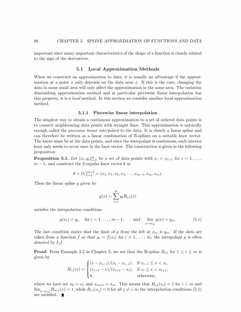
The simplest way to obtain a continuous approximation to a set of ordered data points isto connect neighbouring data points with straight lines. This approximation is naturallyenough called the piecewise linear interpolant to the data. It is clearly a linear spline andcan therefore be written as a linear combination of B-splines on a suitable knot vector.The knots must be at the data points, and since the interpolant is continuous, each interiorknot only needs to occur once in the knot vector. The construction is given in the followingproposition.

Proposition 5.1. Let (xi, yi)mi=1 be a set of data points with xi < xi+1 for i = 1, . . . ,

m− 1, and construct the 2-regular knot vector t as

t = (ti)m+2i=1 = (x1, x1, x2, x3, . . . , xm−1, xm, xm).

Then the linear spline g given by

g(x) =m∑

i=1

yiBi,1(x)

satisfies the interpolation conditions

g(xi) = yi, for i = 1, . . . , m− 1, and limx→x−m

g(x) = ym. (5.1)

The last condition states that the limit of g from the left at xm is ym. If the data aretaken from a function f so that yi = f(xi) for i = 1, . . . , m, the interpolant g is oftendenoted by I1f .

Proof. From Example 2.2 in Chapter 2, we see that the B-spline Bi,1 for 1 ≤ i ≤ m isgiven by

Bi,1(x) =

(x− xi−1)/(xi − xi−1), if xi−1 ≤ x < xi,(xi+1 − x)/(xi+1 − xi), if xi ≤ x < xi+1,0, otherwise,

where we have set x0 = x1 and xm+1 = xm. This means that Bi,1(xi) = 1 for i < m andlimx→x−m

Bm,1(x) = 1, while Bi,1(xj) = 0 for all j 6= i, so the interpolation conditions (5.1)are satisfied.

5.1. LOCAL APPROXIMATION METHODS 99

The piecewise linear interpolant preserves the shape of the data extremely well. Theobvious disadvantage of this approximation is its lack of smoothness.

Intuitively, it seems reasonable that if f is continuous, it should be possible to approx-imate it to within any accuracy by piecewise linear interpolants, if we let the distancebetween the data points become small enough. This is indeed the case. Note that thesymbol Cj [a, b] denotes the set of all functions defined on [a, b] with values in R whosefirst j derivatives are continuous.Proposition 5.2. Suppose that a = x1 < x2 < · · · < xm = b are given points, and set∆x = max1≤i≤m−1{xi+1 − xi}.

1. If f ∈ C[a, b], then for every ε > 0 there is a δ > 0 such that if ∆x < δ, then|f(x)− I1f(x)| < ε for all x ∈ [a, b].

2. If f ∈ C2[a, b] then for all x ∈ [a, b],

|f(x)− (I1f)(x)| ≤ 18(∆x)2 max

a≤z≤b|f ′′(z)|, (5.2)

|f ′(x)− (I1f)′(x)| ≤ 12∆x max

a≤z≤b|f ′′(z)|. (5.3)

Part (i) of Proposition 5.2 states that piecewise linear interpolation to a continuousfunction converges to the function when the distance between the data points goes to zero.More specifically, given a tolerance ε, we can make the error less than the tolerance bychoosing ∆x sufficiently small.

Part (ii) of Proposition 5.2 gives an upper bound for the error in case the function f issmooth, which in this case means that f and its first two derivatives are continuous. Theinequality in (5.2) is often stated as “piecewise linear approximation has approximationorder two”, meaning that ∆x is raised to the power of two in (5.2).

The bounds in Proposition 5.2 depend both on ∆x and the size of the second derivativeof f . Therefore, if the error is not small, it must be because one of these quantities arelarge. If in some way we can find an upper bound M for f ′′, i.e.,

|f ′′(x)| ≤ M, for x ∈ [a, b], (5.4)

we can determine a value of ∆x such that the error, measured as in (5.2), is smaller thansome given tolerance ε. We must clearly require (∆x)2M/8 < ε. This inequality holdsprovided ∆x <

√8ε/M. We conclude that for any ε > 0, we have the implication

∆x <

√8ε

M=⇒ |f(x)− I1f(x)| < ε, for x ∈ [x1, xm]. (5.5)

This estimate tells us how densely we must sample f in order to have error smaller thanε everywhere.

We will on occasions want to compute the piecewise linear interpolant to a given higherdegree spline f . A spline does not necessarily have continuous derivatives, but at least weknow where the discontinuities are. The following proposition is therefore meaningful.Proposition 5.3. Suppose that f ∈ Sd,t for some d and t with interior knots of multiplic-ity at most d (so f is continuous). If the break points (xi)m

i=1 are chosen so as to includeall the knots in t where f ′ is discontinuous, the bounds in (5.2) and (5.3) continue to hold.


5.1.2 Cubic Hermite interpolation

The piecewise linear interpolant has the nice property of being a local construction: Theinterpolant on an interval [xi, xi+1] is completely defined by the value of f at xi and xi+1.The other advantage of f is that it does not oscillate between data points and thereforepreserves the shape of f if ∆x is small enough. In this section we construct an interpolantwhich, unlike the piecewise linear interpolant, has continuous first derivative, and which,like the piecewise linear interpolant, only depends on data values locally. The price ofthe smoothness is that this interpolant requires information about derivatives, and shapepreservation in the strong sense of the piecewise linear interpolant cannot be guaranteed.The interpolant we seek is the solution of the following problem.

Problem 5.4 (Piecewise Cubic Hermite Interpolation). Let the discrete data(xi, f(xi), f ′(xi))m

i=1 with a = x1 < x2 < · · · < xm = b be given. Find a function g = Hfthat satisfies the following conditions:

1. On each subinterval (xi, xi+1) the function g is a cubic polynomial.

2. The given function f is interpolated by g in the sense that

g(xi) = f(xi), and g′(xi) = f ′(xi), for i = 1, . . . , m. (5.6)

A spline g that solves Problem 5.4 must be continuous and have continuous first deriva-tive since two neighbouring pieces meet with the same value f(xi) and first derivative f ′(xi)at a join xi. Since Hf should be a piecewise cubic polynomial, it is natural to try anddefine a knot vector so that Hf can be represented as a linear combination of B-splineson this knot vector. To get the correct smoothness, we need at least a double knot at eachdata point. Since d = 3 and we have 2m interpolation conditions, the length of the knotvector should be 2m + 4, and we might as well choose to use a 4-regular knot vector. Weachieve this by making each interior data point a knot of multiplicity two and place fourknots at the two ends. This leads to the knot vector

t = (ti)2m+4i=1 = (x1, x1, x1, x1, x2, x2, . . . , xm−1, xm−1, xm, xm, xm, xm), (5.7)

which we call the Cubic Hermite knot vector on x = (x1, . . . , xm). This allows us toconstruct the solution to Problem 5.4.

Proposition 5.5. Problem 5.4 has a unique solution Hf in the spline space S3,t, wheret is given in equation (5.7). More specifically, the solution is given by

Hf =2m∑i=1

ciBi,3, (5.8)

where

c2i−1 = f(xi)−13∆xi−1f

′(xi),

c2i = f(xi) +13∆xif

′(xi),

for i = 1, . . . , m, (5.9)

where ∆xj = xj+1−xj , and the points x0 and xm+1 are defined by x0 = x1 and xm+1 = xm.

5.1. LOCAL APPROXIMATION METHODS 101

0.2 0.4 0.6 0.8 1

0.2

0.4

0.6

0.8

1

(a)

0.2 0.4 0.6 0.8 1

0.01

0.02

0.03

0.04

0.05

0.06

(b)

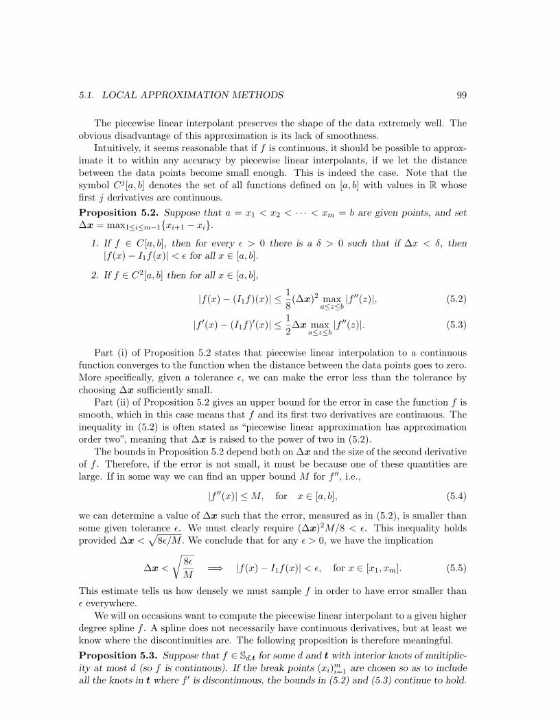
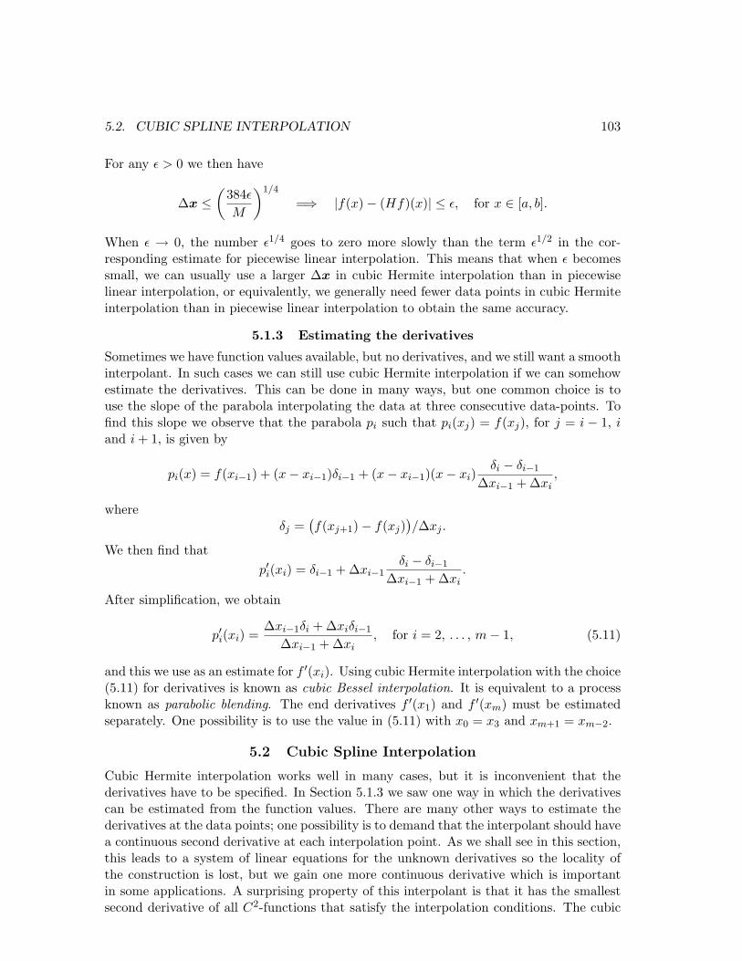
Figure 5.1. Figure (a) shows the cubic Hermite interpolant (solid) to f(x) = x4 (dashed), see Example 5.6, while

the error in this approximation is shown in (b).

Proof. We leave the proof that the spline defined by (5.9) satisfies the interpolationconditions in Problem 5.4 to the reader.

By construction, the solution is clearly a cubic polynomial. That there is only onesolution follows if we can show that the only solution that solves the problem with f(xi) =f ′(xi) = 0 for all i is the function that is zero everywhere. For if the general problem hastwo solutions, the difference between these must solve the problem with all the data equalto zero. If this difference is zero, the two solutions must be equal.

To show that the solution to the problem where all the data are zero is the zerofunction, it is clearly enough to show that the solution is zero in one subinterval. On eachsubinterval the function Hf is a cubic polynomial with value and derivative zero at bothends, and it therefore has four zeros (counting multiplicity) in the subinterval. But theonly cubic polynomial with four zeros is the polynomial that is identically zero. From thiswe conclude that Hf must be zero in each subinterval and therefore identically zero.

Let us see how this method of approximation behaves in a particular situation.Example 5.6. We try to approximate the function f(x) = x4 on the interval [0, 1] with only onepolynomial piece so that m = 2 and [a, b] = [x1, xm] = [0, 1]. Then the cubic Hermite knots are just theBernstein knots. From (5.9) we find (c1, c2, c3, c4) = (0, 0,−1/3, 1), and

(Hf)(x) = −1

33x2(1− x) + x3 = 2x3 − x2.

The two functions f and Hf are shown in Figure 5.1.

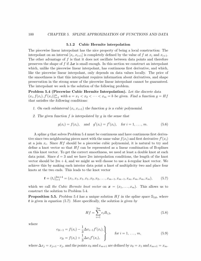
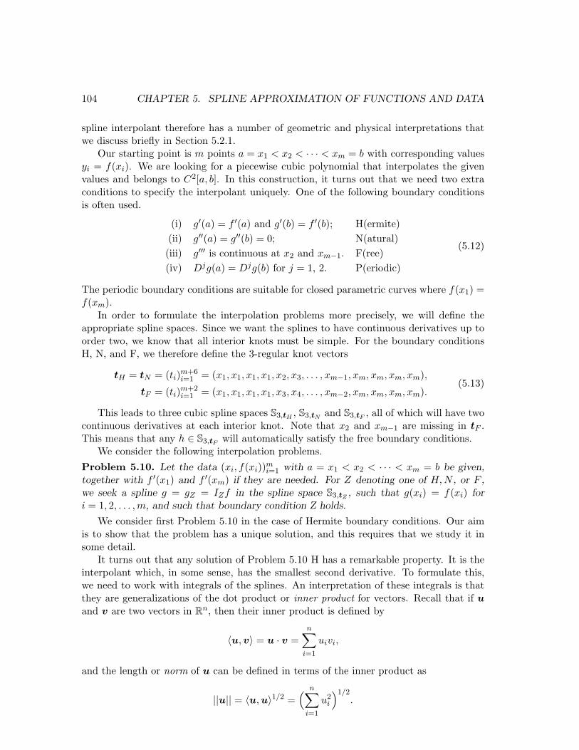
Example 5.7. Let us again approximate f(x) = x4 on [0, 1], but this time we use two polynomial piecesso that m = 3 and x = (0, 1/2, 1). In this case the cubic Hermite knots are t = (0, 0, 0, 0, 1/2, 1/2, 1, 1, 1, 1),and we find the coefficients c = (0, 0,−1/48, 7/48, 1/3, 1). The two functions f and Hf are shown inFigure 5.1 (a). With the extra knots at 1/2 (cf. Example 5.6), we get a much more accurate approximationto x4. In fact, we see from the error plots in Figures 5.1 (b) and 5.1 (b) that the maximum error has beenreduced from 0.06 to about 0.004, a factor of about 15.

Note that in Example 5.6 the approximation becomes negative even though f is non-negative in all of [0, 1]. This shows that in contrast to the piecewise linear interpolant,the cubic Hermite interpolant Hf does not preserve the sign of f . However, it is simpleto give conditions that guarantee Hf to be nonnegative.


0.2 0.4 0.6 0.8 1

0.2

0.4

0.6

0.8

1

(a)

0.2 0.4 0.6 0.8 1

0.001

0.002

0.003

0.004

(b)

Figure 5.2. Figure (a) shows the cubic Hermite interpolant (solid) to f(x) = x4 (dashed) with two polynomial

pieces, see Example 5.7, while the error in the approximation is shown in (b).

Proposition 5.8. Suppose that the function f to be approximated by cubic Hermiteinterpolation satisfies the conditions

f(xi)−13∆xi−1f

′(xi) ≥ 0,

f(xi) +13∆xif

′(xi) ≥ 0,

for i = 1, . . . , m.

Then the cubic Hermite interpolant Hf is nonnegative on [a, b].

Proof. In this case, the spline approximation Hf given by Proposition 5.5 has nonnegativeB-spline coefficients, so that (Hf)(x) for each x is a sum of nonnegative quantities andtherefore nonnegative.

As for the piecewise linear interpolant, it is possible to relate the error to the spacingin x and the size of some derivative of f .Proposition 5.9. Suppose that f has continuous derivatives up to order four on theinterval [x1, xm]. Then

|f(x)− (Hf)(x)| ≤ 1384

(∆x)4 maxa≤z≤b

|f (iv)(z)|, for x ∈ [a, b]. (5.10)

This estimate also holds whenever f is in some spline space Sd,t provided f has a continuousderivative at all the xi.

Proof. See a text on numerical analysis.

The error estimate in (5.10) says that if we halve the distance between the interpolationpoints, then we can expect the error to decrease by a factor of 24 = 16. This is usuallyreferred to as “fourth order convergence”. This behaviour is confirmed by Examples 5.6and 5.7 where the error was reduced by a factor of about 15 when ∆x was halved.

From Proposition 5.9, we can determine a spacing between data points that guaranteesthat the error is smaller than some given tolerance. Suppose that

|f (iv)(x)| ≤ M, for x ∈ [a, b].

5.2. CUBIC SPLINE INTERPOLATION 103

For any ε > 0 we then have

∆x ≤(

384ε

M

)1/4

=⇒ |f(x)− (Hf)(x)| ≤ ε, for x ∈ [a, b].

When ε → 0, the number ε1/4 goes to zero more slowly than the term ε1/2 in the cor-responding estimate for piecewise linear interpolation. This means that when ε becomessmall, we can usually use a larger ∆x in cubic Hermite interpolation than in piecewiselinear interpolation, or equivalently, we generally need fewer data points in cubic Hermiteinterpolation than in piecewise linear interpolation to obtain the same accuracy.

5.1.3 Estimating the derivatives

Sometimes we have function values available, but no derivatives, and we still want a smoothinterpolant. In such cases we can still use cubic Hermite interpolation if we can somehowestimate the derivatives. This can be done in many ways, but one common choice is touse the slope of the parabola interpolating the data at three consecutive data-points. Tofind this slope we observe that the parabola pi such that pi(xj) = f(xj), for j = i − 1, iand i + 1, is given by

pi(x) = f(xi−1) + (x− xi−1)δi−1 + (x− xi−1)(x− xi)δi − δi−1

∆xi−1 + ∆xi,

whereδj =

(f(xj+1)− f(xj)

)/∆xj .

We then find thatp′i(xi) = δi−1 + ∆xi−1

δi − δi−1

∆xi−1 + ∆xi.

After simplification, we obtain

p′i(xi) =∆xi−1δi + ∆xiδi−1

∆xi−1 + ∆xi, for i = 2, . . . , m− 1, (5.11)

and this we use as an estimate for f ′(xi). Using cubic Hermite interpolation with the choice(5.11) for derivatives is known as cubic Bessel interpolation. It is equivalent to a processknown as parabolic blending. The end derivatives f ′(x1) and f ′(xm) must be estimatedseparately. One possibility is to use the value in (5.11) with x0 = x3 and xm+1 = xm−2.

5.2 Cubic Spline Interpolation

Cubic Hermite interpolation works well in many cases, but it is inconvenient that thederivatives have to be specified. In Section 5.1.3 we saw one way in which the derivativescan be estimated from the function values. There are many other ways to estimate thederivatives at the data points; one possibility is to demand that the interpolant should havea continuous second derivative at each interpolation point. As we shall see in this section,this leads to a system of linear equations for the unknown derivatives so the locality ofthe construction is lost, but we gain one more continuous derivative which is importantin some applications. A surprising property of this interpolant is that it has the smallestsecond derivative of all C2-functions that satisfy the interpolation conditions. The cubic


spline interpolant therefore has a number of geometric and physical interpretations thatwe discuss briefly in Section 5.2.1.

Our starting point is m points a = x1 < x2 < · · · < xm = b with corresponding valuesyi = f(xi). We are looking for a piecewise cubic polynomial that interpolates the givenvalues and belongs to C2[a, b]. In this construction, it turns out that we need two extraconditions to specify the interpolant uniquely. One of the following boundary conditionsis often used.

(i) g′(a) = f ′(a) and g′(b) = f ′(b); H(ermite)(ii) g′′(a) = g′′(b) = 0; N(atural)(iii) g′′′ is continuous at x2 and xm−1. F(ree)(iv) Djg(a) = Djg(b) for j = 1, 2. P(eriodic)

(5.12)

The periodic boundary conditions are suitable for closed parametric curves where f(x1) =f(xm).

In order to formulate the interpolation problems more precisely, we will define theappropriate spline spaces. Since we want the splines to have continuous derivatives up toorder two, we know that all interior knots must be simple. For the boundary conditionsH, N, and F, we therefore define the 3-regular knot vectors

tH = tN = (ti)m+6i=1 = (x1, x1, x1, x1, x2, x3, . . . , xm−1, xm, xm, xm, xm),

tF = (ti)m+2i=1 = (x1, x1, x1, x1, x3, x4, . . . , xm−2, xm, xm, xm, xm).

(5.13)

This leads to three cubic spline spaces S3,tH , S3,tN and S3,tF , all of which will have twocontinuous derivatives at each interior knot. Note that x2 and xm−1 are missing in tF .This means that any h ∈ S3,tF will automatically satisfy the free boundary conditions.

We consider the following interpolation problems.Problem 5.10. Let the data (xi, f(xi))m

i=1 with a = x1 < x2 < · · · < xm = b be given,together with f ′(x1) and f ′(xm) if they are needed. For Z denoting one of H,N , or F ,we seek a spline g = gZ = IZf in the spline space S3,tZ , such that g(xi) = f(xi) fori = 1, 2, . . . ,m, and such that boundary condition Z holds.

We consider first Problem 5.10 in the case of Hermite boundary conditions. Our aimis to show that the problem has a unique solution, and this requires that we study it insome detail.

It turns out that any solution of Problem 5.10 H has a remarkable property. It is theinterpolant which, in some sense, has the smallest second derivative. To formulate this,we need to work with integrals of the splines. An interpretation of these integrals is thatthey are generalizations of the dot product or inner product for vectors. Recall that if uand v are two vectors in Rn, then their inner product is defined by

〈u,v〉 = u · v =n∑

i=1

uivi,

and the length or norm of u can be defined in terms of the inner product as

||u|| = 〈u,u〉1/2 =( n∑

i=1

u2i

)1/2.


The corresponding inner product and norm for functions are

〈u, v〉 =∫ b

au(x)v(x)dx =

∫ b

auv

and

||u|| =(∫ b

au(t)2dt

)1/2=

(∫ b

au2

)1/2.

It therefore makes sense to say that two functions u and v are orthogonal if 〈u, v〉 =∫

uv =0.

The first result that we prove says that the error f − IHf is orthogonal to a family oflinear splines.Lemma 5.11. Denote the error in cubic spline interpolation with Hermite end conditionsby e = f − IHf , and let t be the 1-regular knot vector

t = (ti)m+2i=1 = (x1, x1, x2, x3, . . . , xm−1, xm, xm).

Then the second derivative of e is orthogonal to the spline space S1,t. In other words∫ b

ae′′(x)h(x) dx = 0, for all h ∈ S1,t.

Proof. Dividing [a, b] into the subintervals [xi, xi+1] for i = 1, . . . , m − 1, and usingintegration by parts, we find∫ b

ae′′h =

m−1∑i=1

∫ xi+1

xi

e′′h =m−1∑i=1

(e′h

∣∣∣xi+1

xi

−∫ xi+1

xi

e′h′).

Since e′(a) = e′(b) = 0, the first term is zero,

m−1∑i=1

e′h∣∣∣xi+1

xi

= e′(b)h(b)− e′(a)h(a) = 0. (5.14)

For the second term, we observe that since h is a linear spline, its derivative is equalto some constant hi in the subinterval (xi, xi+1), and therefore can be moved outside theintegral. Because of the interpolation conditions we have e(xi+1) = e(xi) = 0, so that

m−1∑i=1

∫ xi+1

xi

e′h′ =m−1∑i=1

hi

∫ xi+1

xi

e′(x) dx = 0.

This completes the proof.

We can now show that the cubic spline interpolant solves a minimization problem. Inany minimization problem, we must specify the space over which we minimize. The spacein this case is EH(f), which is defined in terms of the related space E(f)

E(f) ={g ∈ C2[a, b] | g(xi) = f(xi) for i = 1, . . . , m

},

EH(f) ={g ∈ E(f) | g′(a) = f ′(a) and g′(b) = f ′(b)

}.

(5.15)


The space E(f) is the set of all functions with continuous derivatives up to the secondorder that interpolate f at the data points. If we restrict the derivatives at the ends tocoincide with the derivatives of f we obtain EH(f).

The following theorem shows that the second derivative of a cubic interpolating splinehas the smallest second derivative of all functions in EH(f).Theorem 5.12. Suppose that g = IHf is the solution of Problem 5.10 H. Then∫ b

a

(g′′(x)

)2dx ≤

∫ b

a

(h′′(x)

)2dx for all h in EH(f), (5.16)

with equality if and only if h = g.

Proof. Select some h ∈ EH(f) and set e = h− g. Then we have∫ b

ah′′

2 =∫ b

a

(e′′ + g′′

)2 =∫ b

ae′′

2 + 2∫ b

ae′′g′′ +

∫ b

ag′′

2. (5.17)

Since g ∈ S3,tH we have g′′ ∈ S1,t, where t is the knot vector given in Lemma 5.11. Sinceg = IHh = IHf , we have e = h−IHh so we can apply Lemma 5.11 and obtain

∫ ba e′′g′′ = 0.

We conclude that∫ ba h′′2 ≥

∫ ba g′′2.

To show that we can only have equality in (5.16) when h = g, suppose that∫ ba h′′2 =∫ b

a g′′2. Using (5.17), we observe that we must have∫ ba e′′2 = 0. But since e′′ is continuous,

this means that we must have e′′ = 0. Since we also have e(a) = e′(a) = 0, we concludethat e = 0. This can be shown by using Taylor’s formula

e(x) = e(a) + (x− a)e′(a) +∫ x

ae′′(t)(x− t) dt.

Since e = 0, we end up with g = h.

Lemma 5.11 and Theorem 5.12 allow us to show that the Hermite problem has a uniquesolution.Theorem 5.13. Problem 5.10 H has a unique solution.

Proof. We seek a function

g = IHf =m+2∑i=1

ciBi,3

in S3,tH such that

m+2∑j=1

cjBj,3(xi) = f(xi), for i = 1, . . . , m,

m+2∑j=1

cjB′j,3(xi) = f ′(xi), for i = 1 and m.

(5.18)

This is a linear system of m + 2 equations in the m + 2 unknown B-spline coefficients.From linear algebra we know that such a system has a unique solution if and only if the


corresponding system with zero right-hand side only has the zero solution. This means thatexistence and uniqueness of the solution will follow if we can show that Problem 5.10 Hwith zero data only has the zero solution. Suppose that g ∈ S3,tH solves Problem 5.10 Hwith zero data. Clearly g = 0 is a solution. According to Theorem 5.12, any other solutionmust also minimize the integral of the second derivative. By the uniqueness assertion inTheorem 5.12, we conclude that g = 0 is the only solution.

We have similar results for the “natural” case.

Lemma 5.14. If e = f − INf and t the knot vector

t = (ti)mi=1 = (x1, x2, x3, . . . , xm−1, xm),

the second derivative of e is orthogonal to S1,t,∫ b

ae′′(x)h(x) dx = 0, for all h in S1,t.

Proof. The proof is similar to Lemma 5.11. The relation in (5.14) holds since everyh ∈ S1,t now satisfies h(a) = h(b) = 0.

Lemma 5.14 allows us to prove that the cubic spline interpolation problem with naturalboundary conditions has a unique solution.

Theorem 5.15. Problem 5.10 N has a unique solution g = INf . The solution is theunique function in C2[a, b] with the smallest possible second derivative in the sense that∫ b

a

(g′′(x)

)2dx ≤

∫ b

a

(h′′(x)

)2dx, for all h ∈ E(f),

with equality if and only if h = g.

Proof. The proof of Theorem 5.12 carries over to this case. We only need to observe thatthe natural boundary conditions imply that g′′ ∈ S1,t.

From this it should be clear that the cubic spline interpolants with Hermite and naturalend conditions are extraordinary functions. If we consider all continuous functions withtwo continuous derivatives that interpolate f at the xi, the cubic spline interpolant withnatural end conditions is the one with the smallest second derivative in the sense thatthe integral of the square of the second derivative is minimized. This explains why the Nboundary conditions in (5.12) are called natural. If we restrict the interpolant to have thesame derivative as f at the ends, the solution is still a cubic spline.

For the free end interpolant we will show existence and uniqueness in the next section.No minimization property is known for this spline.

5.2.1 Interpretations of cubic spline interpolation

Today engineers use computers to fit curves through their data points; this is one ofthe main applications of splines. But splines have been used for this purpose long beforecomputers were available, except that at that time the word spline had a different meaning.In industries like for example ship building, a thin flexible ruler was used to draw curves.


The ruler could be clamped down at fixed data points and would then take on a nicesmooth shape that interpolated the data and minimized the bending energy in accordancewith the physical laws. This allowed the user to interpolate the data in a visually pleasingway. This flexible ruler was known as a draftmans spline.

The physical laws governing the classical spline used by ship designers tell us thatthe ruler will take on a shape that minimizes the total bending energy. The linearizedbending energy is given by

∫g′′2, where g(x) is the position of the centerline of the ruler.

Outside the first and last fixing points the ruler is unconstrained and will take the shapeof a straight line. From this we see that the natural cubic spline models such a linearizedruler. The word spline was therefore a natural choice for the cubic interpolants we haveconsidered here when they were first studied systematically in 1940’s.

The cubic spline interpolant also has a related, geometric interpretation. From differ-ential geometry we know that the curvature of a function g(x) is given by

κ(x) =g′′(x)(

1 + (g′(x))2)3/2

.

The curvature κ(x) measures how much the function curves at x and is important in thestudy of parametric curves. If we assume that 1+g′2 ≈ 1 on [a, b], then κ(x) ≈ g′′(x). Thecubic spline interpolants IHf and INf can therefore be interpreted as the interpolantswith the smallest linearized curvature.

5.2.2 Numerical solution and examples

If we were just presented with the problem of finding the C2 function that interpolate agiven function at some points and have the smallest second derivative, without the knowl-edge that we obtained in Section 5.2, we would have to work very hard to write a reliablecomputer program that could solve the problem. With Theorem 5.15, the most difficultpart of the work has been done, so that in order to compute the solution to say Prob-lem 5.10 H, we only have to solve the linear system of equations (5.18). Let us take acloser look at this system. We order the equations so that the boundary conditions cor-respond to the first and last equation, respectively. Because of the local support propertyof the B-splines, only a few unknowns appear in each equation, in other words we have abanded linear system. Indeed, since ti+3 = xi, we see that only {Bj,3}i+3

j=i can be nonzeroat xi. But we note also that xi is located at the first knot of Bi+3,3, which means thatBi+3,3(xi) = 0. Since we also havet B′

j,3(x1) = 0 for j ≥ 3 and B′j,3(xm) = 0 for j ≤ m,

we conclude that the system can be written in the tridiagonal form

Ac =

α1 γ1

β2 α2 γ2

. . . . . . . . .βm+1 αm+1 γm+1

βm+2 αm+2

c1

c2...

cm+1

cm+2

=

f ′(x1)f(x1)

...f(xm)f ′(xm)

= f , (5.19)

where the elements of A are given by

α1 = B′1,3(x1), αm+2 = B′

m+2,3(xm),

γ1 = B′2,3(x1), βm+2 = B′

m+1,3(xm),

βi+1 = Bi,3(xi), αi+1 = Bi+1,3(xi), γi+1 = Bi+2,3(xi).

(5.20)


1 2 3 4 5 6 7

0.2

0.4

0.6

0.8

1

(a)

5 10 15 20

0.2

0.4

0.6

0.8

1

(b)

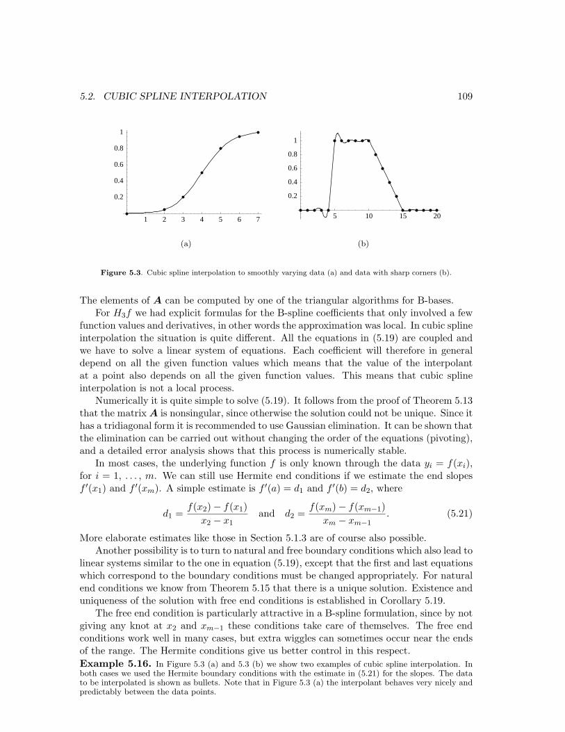
Figure 5.3. Cubic spline interpolation to smoothly varying data (a) and data with sharp corners (b).

The elements of A can be computed by one of the triangular algorithms for B-bases.For H3f we had explicit formulas for the B-spline coefficients that only involved a few

function values and derivatives, in other words the approximation was local. In cubic splineinterpolation the situation is quite different. All the equations in (5.19) are coupled andwe have to solve a linear system of equations. Each coefficient will therefore in generaldepend on all the given function values which means that the value of the interpolantat a point also depends on all the given function values. This means that cubic splineinterpolation is not a local process.

Numerically it is quite simple to solve (5.19). It follows from the proof of Theorem 5.13that the matrix A is nonsingular, since otherwise the solution could not be unique. Since ithas a tridiagonal form it is recommended to use Gaussian elimination. It can be shown thatthe elimination can be carried out without changing the order of the equations (pivoting),and a detailed error analysis shows that this process is numerically stable.

In most cases, the underlying function f is only known through the data yi = f(xi),for i = 1, . . . , m. We can still use Hermite end conditions if we estimate the end slopesf ′(x1) and f ′(xm). A simple estimate is f ′(a) = d1 and f ′(b) = d2, where

d1 =f(x2)− f(x1)

x2 − x1and d2 =

f(xm)− f(xm−1)xm − xm−1

. (5.21)

More elaborate estimates like those in Section 5.1.3 are of course also possible.Another possibility is to turn to natural and free boundary conditions which also lead to

linear systems similar to the one in equation (5.19), except that the first and last equationswhich correspond to the boundary conditions must be changed appropriately. For naturalend conditions we know from Theorem 5.15 that there is a unique solution. Existence anduniqueness of the solution with free end conditions is established in Corollary 5.19.

The free end condition is particularly attractive in a B-spline formulation, since by notgiving any knot at x2 and xm−1 these conditions take care of themselves. The free endconditions work well in many cases, but extra wiggles can sometimes occur near the endsof the range. The Hermite conditions give us better control in this respect.Example 5.16. In Figure 5.3 (a) and 5.3 (b) we show two examples of cubic spline interpolation. Inboth cases we used the Hermite boundary conditions with the estimate in (5.21) for the slopes. The datato be interpolated is shown as bullets. Note that in Figure 5.3 (a) the interpolant behaves very nicely andpredictably between the data points.


In comparison, the interpolant in Figure 5.3 (b) has some unexpected wiggles. This is a characteristicfeature of spline interpolation when the data have sudden changes or sharp corners. For such data, leastsquares approximation by splines usually gives better results, see Section 5.3.2.

5.3 General Spline Approximation

So far, we have mainly considered spline approximation methods tailored to specific de-grees. In practice, cubic splines are undoubtedly the most common, but there is an obviousadvantage to have methods available for splines of all degrees. In this section we first con-sider spline interpolation for splines of arbitrary degree. The optimal properties of thecubic spline interpolant can be generalized to spline interpolants of any odd degree, buthere we only focus on the practical construction of the interpolant. Least squares approxi-mation, which we study in Section 5.3.2, is a completely different approximation procedurethat often give better results than interpolation, especially when the data changes abruptlylike in Figure 1.6 (b).

5.3.1 Spline interpolation

Given points (xi, yi)mi=1, we again consider the problem of finding a spline g such that

g(xi) = yi, i = 1, . . . ,m.

In the previous section we used cubic splines where the knots of the spline were locatedat the data points. This works well if the data points are fairly evenly spaced, but canotherwise give undesirable effects. In such cases the knots should not be chosen at thedata points. However, how to choose good knots in general is difficult.

In some cases we might also be interested in doing interpolation with splines of degreehigher than three. We could for example be interested in a smooth representation of thesecond derivative of f . However, if we want f ′′′ to be continuous, say, then the degree dmust be higher than three. We therefore consider the following interpolation problem.Problem 5.17. Let there be given data

(xi, yi

)m

i=1and a spline space Sd,t whose knot

vector t = (ti)m+d+1i=1 satisfies ti+d+1 > ti, for i = 1, . . . , m. Find a spline g in Sd,t such

that

g(xi) =m∑

j=1

cjBj,d(xi) = yi, for i = 1, . . . , m. (5.22)

The equations in (5.22) form a system of m equations in m unknowns. In matrix formthese equations can be written

Ac =

B1,d(x1) . . . Bm,d(x1)...

. . ....

B1,d(xm) . . . Bm,d(xm)

c1

...cm

=

y1...

ym

= y. (5.23)

Theorem 5.18 gives necessary and sufficient conditions for this system to have a uniquesolution, in other words for A to be nonsingular.Theorem 5.18. The matrix A in (5.23) is nonsingular if and only if the diagonal elementsai,i = Bi,d(xi) are positive for i = 1, . . . m.

Proof. See Theorem 9.6 in Chapter 9.

5.3. GENERAL SPLINE APPROXIMATION 111

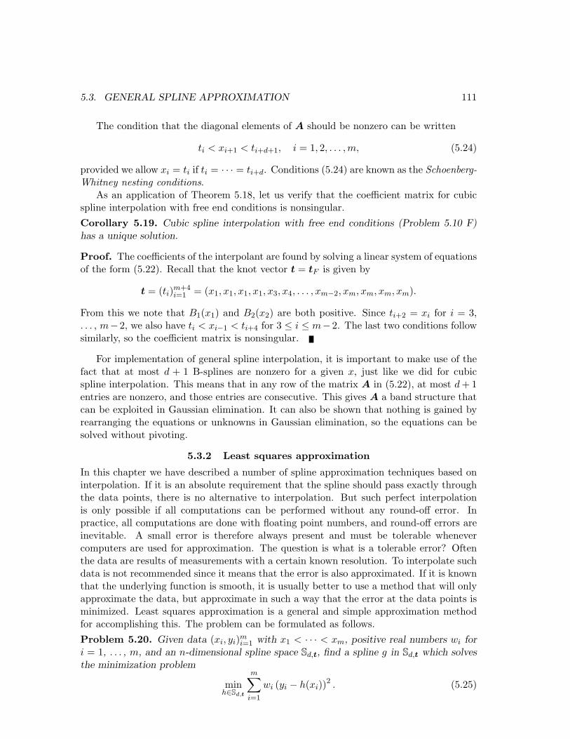
The condition that the diagonal elements of A should be nonzero can be written

ti < xi+1 < ti+d+1, i = 1, 2, . . . ,m, (5.24)

provided we allow xi = ti if ti = · · · = ti+d. Conditions (5.24) are known as the Schoenberg-Whitney nesting conditions.

As an application of Theorem 5.18, let us verify that the coefficient matrix for cubicspline interpolation with free end conditions is nonsingular.Corollary 5.19. Cubic spline interpolation with free end conditions (Problem 5.10 F)has a unique solution.

Proof. The coefficients of the interpolant are found by solving a linear system of equationsof the form (5.22). Recall that the knot vector t = tF is given by

t = (ti)m+4i=1 = (x1, x1, x1, x1, x3, x4, . . . , xm−2, xm, xm, xm, xm).

From this we note that B1(x1) and B2(x2) are both positive. Since ti+2 = xi for i = 3,. . . , m−2, we also have ti < xi−1 < ti+4 for 3 ≤ i ≤ m−2. The last two conditions followsimilarly, so the coefficient matrix is nonsingular.

For implementation of general spline interpolation, it is important to make use of thefact that at most d + 1 B-splines are nonzero for a given x, just like we did for cubicspline interpolation. This means that in any row of the matrix A in (5.22), at most d + 1entries are nonzero, and those entries are consecutive. This gives A a band structure thatcan be exploited in Gaussian elimination. It can also be shown that nothing is gained byrearranging the equations or unknowns in Gaussian elimination, so the equations can besolved without pivoting.

5.3.2 Least squares approximation

In this chapter we have described a number of spline approximation techniques based oninterpolation. If it is an absolute requirement that the spline should pass exactly throughthe data points, there is no alternative to interpolation. But such perfect interpolationis only possible if all computations can be performed without any round-off error. Inpractice, all computations are done with floating point numbers, and round-off errors areinevitable. A small error is therefore always present and must be tolerable whenevercomputers are used for approximation. The question is what is a tolerable error? Oftenthe data are results of measurements with a certain known resolution. To interpolate suchdata is not recommended since it means that the error is also approximated. If it is knownthat the underlying function is smooth, it is usually better to use a method that will onlyapproximate the data, but approximate in such a way that the error at the data points isminimized. Least squares approximation is a general and simple approximation methodfor accomplishing this. The problem can be formulated as follows.Problem 5.20. Given data (xi, yi)m

i=1 with x1 < · · · < xm, positive real numbers wi fori = 1, . . . , m, and an n-dimensional spline space Sd,t, find a spline g in Sd,t which solvesthe minimization problem

minh∈Sd,t

m∑i=1

wi (yi − h(xi))2 . (5.25)


The expression (5.25) that is minimized is a sum of the squares of the errors at eachdata point, weighted by the numbers wi which are called weights. This explains the nameleast squares approximation, or more precisely weighted least squares approximation. If wi

is large in comparison to the other weights, the error yi − h(xi) will count more in theminimization. As the the weight grows, the error at this data point will go to zero. Onthe other hand, if the weight is small in comparison to the other weights, the error at thatdata point gives little contribution to the total least squares deviation. If the weight iszero, the approximation is completely independent of the data point. Note that the actualvalue of the weights is irrelevant, it is the relative size that matters. The weights thereforeprovides us with the opportunity to attach a measure of confidence to each data point.If we know that yi is a very accurate data value we can give it a large weight, while if yi

is very inaccurate we can give it a small weight. Note that it is the relative size of theweights that matters, a natural ‘neutral’ value is therefore wi = 1.

From our experience with interpolation, we see that if we choose the spline space Sd,t

so that the number of B-splines equals the number of data points and such that Bi(xi) > 0for all i, then the least squares approximation will agree with the interpolant and give zeroerror, at least in the absence of round off errors. Since the whole point of introducing theleast squares approximation is to avoid interpolation of the data, we must make sure thatn is smaller than m and that the knot vector is appropriate. This all means that thespline space Sd,t must be chosen appropriately, but this is not easy. Of course we wouldlike the spline space to be such that a “good” approximation g can be found. Good, willhave different interpretations for different applications. A statistician would like g to havecertain statistical properties. A designer would like an aesthetically pleasing curve, andmaybe some other shape and tolerance requirements to be satisfied. In practice, one oftenstarts with a small spline space, and then adds knots in problematic areas until hopefullya satisfactory approximation is obtained.

Different points of view are possible in order to analyze Problem 5.20 mathematically.Our approach is based on linear algebra. Our task is to find the vector c = (c1, . . . , cn)of B-spline coefficients of the spline g solving Problem 5.20. The following matrix-vectorformulation is convenient.

Lemma 5.21. Problem 5.20 is equivalent to the linear least squares problem

minc∈Rn

‖Ac− b‖2,

where A ∈ Rm,n and b ∈ Rm have components

ai,j =√

wiBj(xi) and bi =√

wiyi, (5.26)

and for any u = (u1, . . . , um),

‖u‖ =√

u21 + · · ·+ u2

m,

is the usual Euclidean length of a vector in Rm.

5.3. GENERAL SPLINE APPROXIMATION 113

Proof. Suppose c = (c1, . . . , cn) are the B-spline coefficients of some h ∈ Sd,t. Then

‖Ac− b‖22 =

m∑i=1

( n∑j=1

ai,jcj − bi

)2

=m∑

i=1

( n∑j=1

√wiBj(xi)cj −

√wiyi

)2

=m∑

i=1

wi

(h(xi)− yi

)2.

This shows that the two minimization problems are equivalent.

In the next lemma, we collect some facts about the general linear least squares problem.Recall that a symmetric matrix N is positive semidefinite if cT Nc ≥ 0 for all c ∈ Rn,and positive definite if in addition cT Nc > 0 for all nonzero c ∈ Rn.Lemma 5.22. Suppose m and n are positive integers with m ≥ n, and let the matrix Ain Rm,n and the vector b in Rm be given. The linear least squares problem

minc∈Rn

‖Ac− b‖2 (5.27)

always has a solution c∗ which can be found by solving the linear set of equations

AT Ac∗ = AT b. (5.28)

The coefficient matrix N = AT A is symmetric and positive semidefinite. It is positivedefinite, and therefore nonsingular, and the solution of (5.27) is unique if and only if Ahas linearly independent columns.

Proof. Let span(A) denote the n-dimensional linear subspace of Rm spanned by thecolumns of A,

span(A) = {Ac | c ∈ Rn}.

From basic linear algebra we know that a vector b ∈ Rm can be written uniquely as a sumb = b1 + b2, where b1 is a linear combination of the columns of A so that b1 ∈ span(A),and b2 is orthogonal to span(A), i.e., we have bT

2 d = 0 for all d in span(A). Using thisdecomposition of b, and the Pythagorean theorem, we have for any c ∈ Rn,

‖Ac− b‖2 = ‖Ac− b1 − b2‖2 = ‖Ac− b1‖2 + ‖b2‖2.

It follows that ‖Ac − b‖22 ≥ ‖b2‖2

2 for any c ∈ Rn, with equality if Ac = b1. A c = c∗

such that Ac∗ = b1 clearly exists since b1 is in span(A), and c∗ is unique if and only ifA has linearly independent columns. To derive the linear system for c∗, we note that anyc that is minimizing satisfies Ac− b = −b2. Since we also know that b2 is orthogonal tospan(A), we must have

dT (Ac− b) = cT1 AT (Ac− b) = 0

for all d = Ac1 in span(A), i.e., for all c1 in Rn. But this is only possible if AT (Ac−b) = 0.This proves (5.28).


5 10 15 20

0.250.5

0.751

1.251.5

1.752

(a)

5 10 15 20

0.250.5

0.751

1.251.5

1.752

(b)

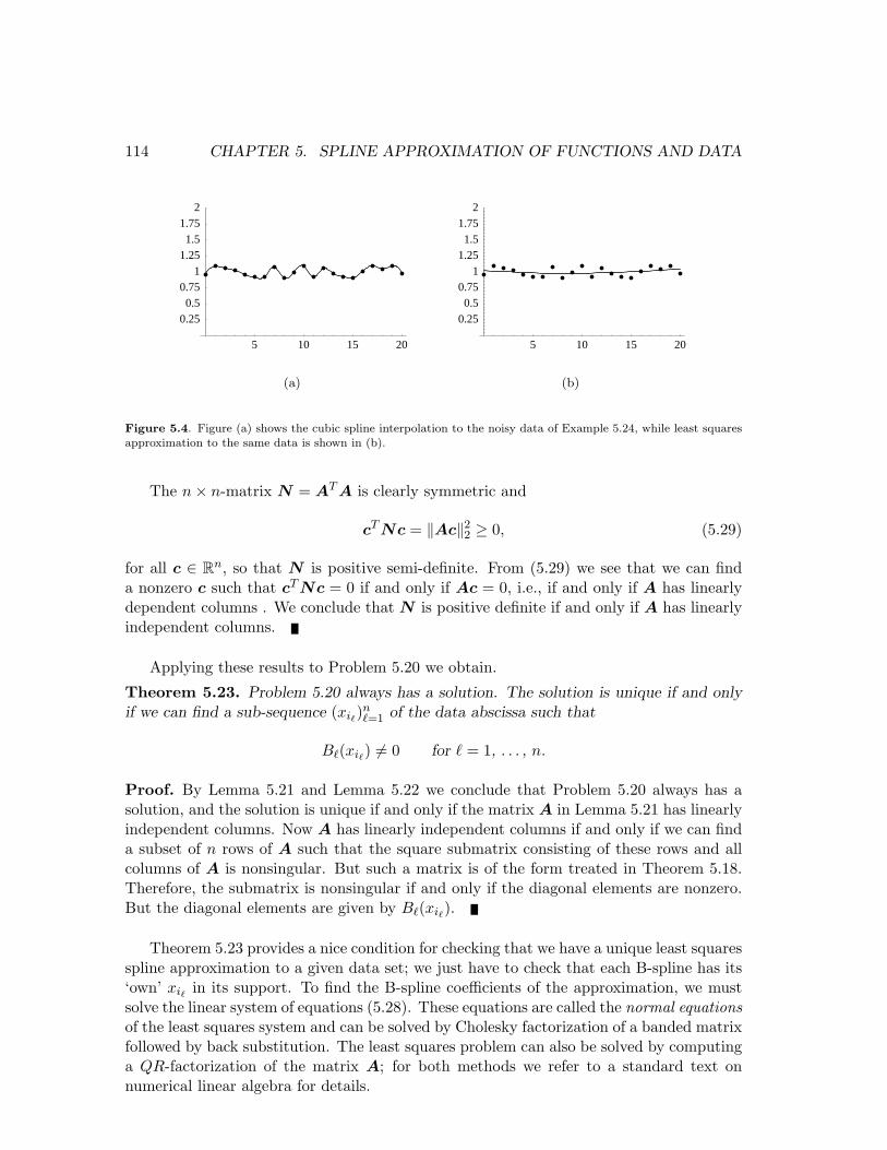
Figure 5.4. Figure (a) shows the cubic spline interpolation to the noisy data of Example 5.24, while least squaresapproximation to the same data is shown in (b).

The n× n-matrix N = AT A is clearly symmetric and

cT Nc = ‖Ac‖22 ≥ 0, (5.29)

for all c ∈ Rn, so that N is positive semi-definite. From (5.29) we see that we can finda nonzero c such that cT Nc = 0 if and only if Ac = 0, i.e., if and only if A has linearlydependent columns . We conclude that N is positive definite if and only if A has linearlyindependent columns.

Applying these results to Problem 5.20 we obtain.

Theorem 5.23. Problem 5.20 always has a solution. The solution is unique if and onlyif we can find a sub-sequence (xi`)

n`=1 of the data abscissa such that

B`(xi`) 6= 0 for ` = 1, . . . , n.

Proof. By Lemma 5.21 and Lemma 5.22 we conclude that Problem 5.20 always has asolution, and the solution is unique if and only if the matrix A in Lemma 5.21 has linearlyindependent columns. Now A has linearly independent columns if and only if we can finda subset of n rows of A such that the square submatrix consisting of these rows and allcolumns of A is nonsingular. But such a matrix is of the form treated in Theorem 5.18.Therefore, the submatrix is nonsingular if and only if the diagonal elements are nonzero.But the diagonal elements are given by B`(xi`).

Theorem 5.23 provides a nice condition for checking that we have a unique least squaresspline approximation to a given data set; we just have to check that each B-spline has its‘own’ xi` in its support. To find the B-spline coefficients of the approximation, we mustsolve the linear system of equations (5.28). These equations are called the normal equationsof the least squares system and can be solved by Cholesky factorization of a banded matrixfollowed by back substitution. The least squares problem can also be solved by computinga QR-factorization of the matrix A; for both methods we refer to a standard text onnumerical linear algebra for details.

5.4. THE VARIATION DIMINISHING SPLINE APPROXIMATION 115

Example 5.24. Least squares approximation is especially appropriate when the data is known to benoisy. Consider the data represented as bullets in Figure 5.4 (a). These data were obtained by addingrandom perturbations in the interval [−0.1, 0.1] to the function f(x) = 1. In Figure 5.4 (a) we showthe cubic spline interpolant (with free end conditions) to the data, while Figure 5.4 (b) shows the cubicleast squares approximation to the same data, using no interior knots. We see that the least squaresapproximation smoothes out the data nicely. We also see that the cubic spline interpolant gives a niceapproximation to the given data, but it also reproduces the noise that was added artificially.

Once we have made the choice of approximating the data in Example 5.24 using cubicsplines with no interior knots, we have no chance of representing the noise in the data.The flexibility of cubic polynomials is nowhere near rich enough to represent all the os-cillations that we see in Figure 5.4 (a), and this gives us the desired smoothing effect inFigure 5.4 (b). The advantage of the method of least squares is that it gives a reasonablysimple method for computing a reasonably good approximation to quite arbitrary data onquite arbitrary knot vectors. But it is largely the knot vector that decides how much theapproximation is allowed to oscillate, and good methods for choosing the knot vector istherefore of fundamental importance. Once the knot vector is given there are in fact manyapproximation methods that will provide good approximations.

5.4 The Variation Diminishing Spline Approximation

In this section we describe a simple, but very useful method for obtaining spline approx-imations to a function f defined on an interval [a, b]. This method is a generalization ofpiecewise linear interpolation and has a nice shape preserving behaviour. For example, ifthe function f is positive, then the spline approximation will also be positive.Definition 5.25. Let f be a given continuous function on the interval [a, b], let d be agiven positive integer, and let t = (t1, . . . , tn+d+1) be a d + 1-regular knot vector withboundary knots td+1 = a and tn+1 = b. The spline given by

(V f)(x) =n∑

j=1

f(t∗j )Bj,d(x) (5.30)

where t∗j = (tj+1 + · · ·+ tj+d)/d are the knot averages, is called the Variation DiminishingSpline Approximation of degree d to f on the knot vector t.

The approximation method that assigns to f the spline approximation V f is aboutthe simplest method of approximation that one can imagine. Unlike some of the othermethods discussed in this chapter there is no need to solve a linear sustem. To obtain V f ,we simply evaluate f at certain points and use these function values as B-spline coefficientsdirectly.

Note that if all interior knots occur less than d + 1 times in t, then

a = t∗1 < t∗2 < . . . < t∗n−1 < t∗n = b. (5.31)

This is because t1 and tn+d+1 do not occur in the definition of t∗1 and t∗n so that all selectionsof d consecutive knots must be different.Example 5.26. Suppose that d = 3 and that the interior knots of t are uniform in the interval [0, 1],say

t = (0, 0, 0, 0, 1/m, 2/m, . . . , 1− 1/m, 1, 1, 1, 1). (5.32)

For m ≥ 2 we then have

t∗ = (0, 1/(3m), 1/m, 2/m, . . . , 1− 1/m, 1− 1/(3m), 1). (5.33)


0.2 0.4 0.6 0.8 1

1.25

1.5

1.75

2

2.25

2.5

2.75

(a)

0.2 0.4 0.6 0.8 1

0.005

0.01

0.015

0.02

0.025

(b)

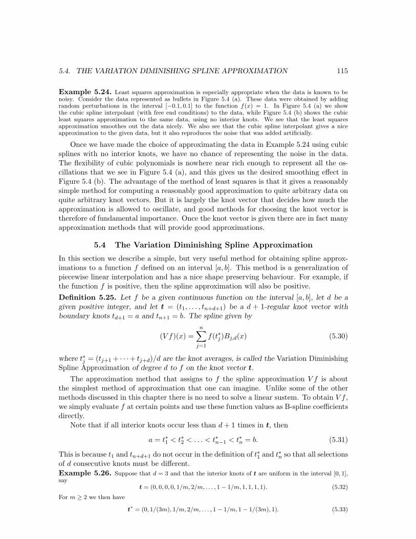
Figure 5.5. The exponential function together with the cubic variation diminishing approximation of Example 5.26in the special case m = 5 is shown in (a). The error in the approximation is shown in (b).

Figure 5.5 (a) shows the cubic variation diminishing approximation to the exponential function on theknot vector in (5.32) with m = 5, and the error is shown in Figure 5.5 (b). The error is so small that it isdifficult to distinguish between the two functions in Figure 5.5 (a).

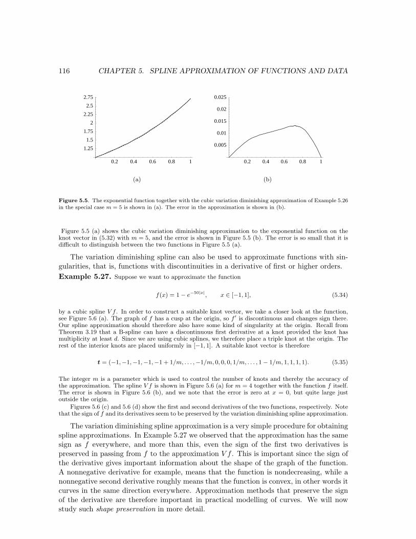
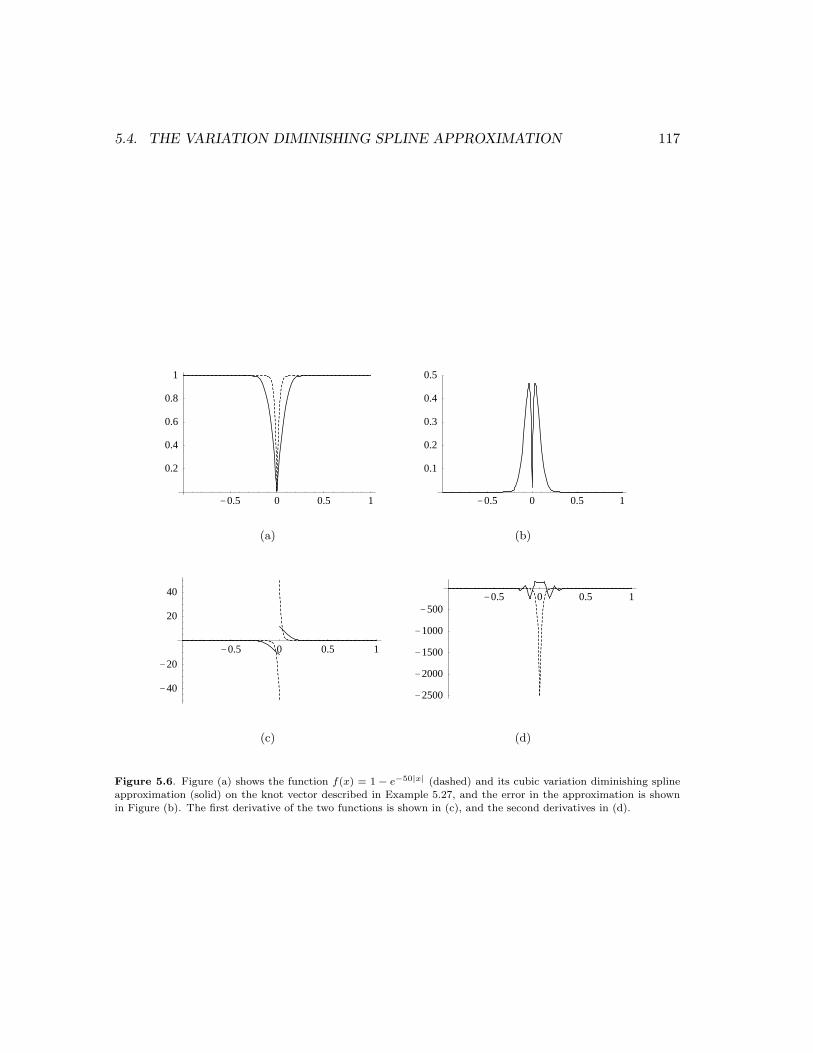
The variation diminishing spline can also be used to approximate functions with sin-gularities, that is, functions with discontinuities in a derivative of first or higher orders.Example 5.27. Suppose we want to approximate the function

f(x) = 1− e−50|x|, x ∈ [−1, 1], (5.34)

by a cubic spline V f . In order to construct a suitable knot vector, we take a closer look at the function,see Figure 5.6 (a). The graph of f has a cusp at the origin, so f ′ is discontinuous and changes sign there.Our spline approximation should therefore also have some kind of singularity at the origin. Recall fromTheorem 3.19 that a B-spline can have a discontinuous first derivative at a knot provided the knot hasmultiplicity at least d. Since we are using cubic splines, we therefore place a triple knot at the origin. Therest of the interior knots are placed uniformly in [−1, 1]. A suitable knot vector is therefore

t = (−1,−1,−1,−1,−1 + 1/m, . . . ,−1/m, 0, 0, 0, 1/m, . . . , 1− 1/m, 1, 1, 1, 1). (5.35)

The integer m is a parameter which is used to control the number of knots and thereby the accuracy ofthe approximation. The spline V f is shown in Figure 5.6 (a) for m = 4 together with the function f itself.The error is shown in Figure 5.6 (b), and we note that the error is zero at x = 0, but quite large justoutside the origin.

Figures 5.6 (c) and 5.6 (d) show the first and second derivatives of the two functions, respectively. Notethat the sign of f and its derivatives seem to be preserved by the variation diminishing spline approximation.

The variation diminishing spline approximation is a very simple procedure for obtainingspline approximations. In Example 5.27 we observed that the approximation has the samesign as f everywhere, and more than this, even the sign of the first two derivatives ispreserved in passing from f to the approximation V f . This is important since the sign ofthe derivative gives important information about the shape of the graph of the function.A nonnegative derivative for example, means that the function is nondecreasing, while anonnegative second derivative roughly means that the function is convex, in other words itcurves in the same direction everywhere. Approximation methods that preserve the signof the derivative are therefore important in practical modelling of curves. We will nowstudy such shape preservation in more detail.


-0.5 0 0.5 1

0.2

0.4

0.6

0.8

1

(a)

-0.5 0 0.5 1

0.1

0.2

0.3

0.4

0.5

(b)

-0.5 0 0.5 1

-40

-20

20

40

(c)

-0.5 0 0.5 1

-2500

-2000

-1500

-1000

-500

(d)

Figure 5.6. Figure (a) shows the function f(x) = 1 − e−50|x| (dashed) and its cubic variation diminishing splineapproximation (solid) on the knot vector described in Example 5.27, and the error in the approximation is shown

in Figure (b). The first derivative of the two functions is shown in (c), and the second derivatives in (d).


5.4.1 Preservation of bounds on a function

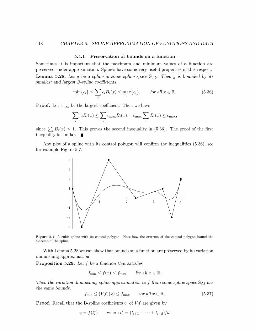
Sometimes it is important that the maximum and minimum values of a function arepreserved under approximation. Splines have some very useful properties in this respect.Lemma 5.28. Let g be a spline in some spline space Sd,t. Then g is bounded by itssmallest and largest B-spline coefficients,

mini{ci} ≤

∑i

ciBi(x) ≤ maxi{ci}, for all x ∈ R. (5.36)

Proof. Let cmax be the largest coefficient. Then we have∑i

ciBi(x) ≤∑

i

cmaxBi(x) = cmax

∑i

Bi(x) ≤ cmax,

since∑

i Bi(x) ≤ 1. This proves the second inequality in (5.36). The proof of the firstinequality is similar.

Any plot of a spline with its control polygon will confirm the inequalities (5.36), seefor example Figure 5.7.

1 2 3 4

-3

-2

-1

1

2

3

4

Figure 5.7. A cubic spline with its control polygon. Note how the extrema of the control polygon bound the

extrema of the spline.

With Lemma 5.28 we can show that bounds on a function are preserved by its variationdiminishing approximation.Proposition 5.29. Let f be a function that satisfies

fmin ≤ f(x) ≤ fmax for all x ∈ R.

Then the variation diminishing spline approximation to f from some spline space Sd,t hasthe same bounds,

fmin ≤ (V f)(x) ≤ fmax for all x ∈ R. (5.37)

Proof. Recall that the B-spline coefficients ci of V f are given by

ci = f(t∗i ) where t∗i = (ti+1 + · · ·+ ti+d)/d.


We therefore have that all the B-spline coefficients of V f are bounded below by fmin andabove by fmax. The inequalities in (5.37) therefore follow as in Lemma 5.28.

5.4.2 Preservation of monotonicity

Many geometric properties of smooth functions can be characterized in terms of the deriva-tive of the function. In particular, the sign of the derivative tells us whether the functionis increasing or decreasing. The variation diminishing approximation also preserves infor-mation about the derivatives in a very convenient way. Let us first define exactly what wemean by increasing and decreasing functions.

Definition 5.30. A function f defined on an interval [a, b] is increasing if the inequalityf(x0) ≤ f(x1) holds for all x0 and x1 in [a, b] with x0 < x1. It is decreasing if f(x0) ≥ f(x1)for all x0 and x1 in [a, b] with x0 < x1. A function that is increasing or decreasing is saidto be monotone.

The two properties of being increasing and decreasing are clearly completely symmetricand we will only prove results about increasing functions.

If f is differentiable, monotonicity can be characterized in terms of the derivative.

Proposition 5.31. A differentiable function is increasing if and only if its derivative isnonnegative.

Proof. Suppose that f is increasing. Then (f(x + h)− f(x))/h ≥ 0 for all x and positiveh such that both x and x + h are in [a, b]. Taking the limit as h tends to zero, we musthave f ′(x) ≥ 0 for an increasing differentiable function. At x = b a similar argument withnegative h may be used.

If the derivative of f is nonnegative, let x0 and x1 be two distinct points in [a, b] withx0 < x1. The mean value theorem then states that

f(x1)− f(x0)x1 − x0

= f ′(θ)

for some θ ∈ (x0, x1). Since f ′(θ) ≥ 0, we conclude that f(x1) ≥ f(x0).

Monotonicity of a spline can be characterized in terms of some simple conditions onits B-spline coefficients.

Proposition 5.32. Let t be a d + 1-extended knot vector for splines on the interval[a, b] = [td+1, tn+1], and let g =

∑ni=1 ciBi be a spline in Sd,t. If the coefficients are

increasing, that is ci ≤ ci+1 for i = 1, . . . , n − 1, then g is increasing. If the coefficientsare decreasing then g is decreasing.

Proof. The proposition is certainly true for d = 0, so we can assume that d ≥ 1. Supposefirst that there are no interior knots in t of multiplicity d + 1. If we differentiate g we findg′(x) =

∑ni=1 ∆ciBi,d−1(x) for x ∈ [a, b], where

∆ci = dci − ci−1

ti+d − ti.

Since all the coefficients of g′ are nonnegative we must have g′(x) ≥ 0 (really the one sidedderivative from the right) for x ∈ [a, b]. Since we have assumed that there are no knots


of multiplicity d + 1 in (a, b), we know that g is continuous and hence that it must beincreasing.

If there is an interior knot at ti = ti+d of multiplicity d+1, we conclude from the abovethat g is increasing on both sides of ti. But we also know that g(ti) = ci while the limit ofg from the left is ci−1. The jump is therefore ci − ci−1 which is nonnegative so g increasesacross the jump.

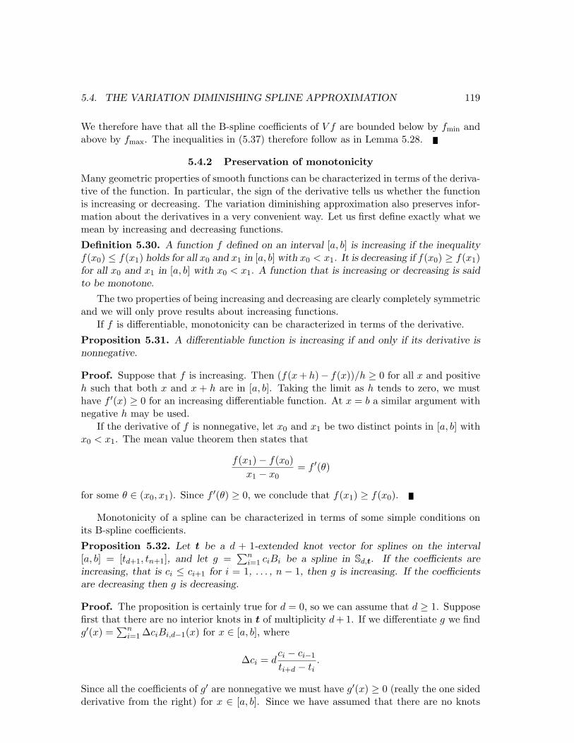
An example of an increasing spline with its control polygon is shown in Figure 5.8 (a).Its derivative is shown in Figure 5.8 (b) and is, as expected, positive.

1 2 3 4

-1

1

2

3

(a)

1 2 3 4

0.5

1

1.5

2

2.5

3

(b)

Figure 5.8. An increasing cubic spline (a) and its derivative (b).

From Proposition 5.32 it is now easy to deduce that V f preserves monotonicity in f .Proposition 5.33. Let f be function defined on the interval [a, b] and let t be a d + 1-extended knot vector with td+1 = a and tn+1 = b. If f is increasing (decreasing) on [a, b],then the variation diminishing approximation V f is also increasing (decreasing) on [a, b].

Proof. The variation diminishing approximation V f has as its i’th coefficient ci = f(t∗i ),and since f is increasing these coefficients are also increasing. Proposition 5.32 then showsthat V f is increasing.

That V f preserves monotonicity means that the oscillations we saw could occur inspline interpolation are much less pronounced in the variation diminishing spline approxi-mation. In fact, we shall also see that V f preserves the sign of the second derivative of fwhich reduces further the possibility of oscillations.

5.4.3 Preservation of convexity

From elementary calculus, we know that the sign of the second derivative of a functiontells us in whether the function curves upwards or downwards, or whether the functionis convex or concave. These concepts can be defined for functions that have no a priorismoothness.Definition 5.34. A function f is said to be convex on an interval (a, b) if

f((1− λ)x0 + λx2

)≤ (1− λ)f(x0) + λf(x2) (5.38)

for all x0 and x2 in [a, b] and for all λ in [0, 1]. If −f is convex then f is said to be concave.


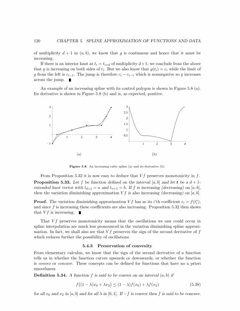
Figure 5.9. A convex function and the cord connecting two points on the graph.

From Definition 5.34 we see that f is convex if the line between two points on thegraph of f is always above the graph, see Figure 5.9. It therefore ‘curves upwards’ justlike smooth functions with nonnegative second derivative.

Convexity can be characterized in many different ways, some of which are listed in thefollowing lemma.

Lemma 5.35. Let f be a function defined on the open interval (a, b).

1. The function f is convex if and only if

f(x1)− f(x0)x1 − x0

≤ f(x2)− f(x1)x2 − x1

(5.39)

for all x0, x1 and x2 in (a, b) with x0 < x1 < x2.

2. If f is differentiable on (a, b), it is convex if and only if f ′(y0) ≤ f ′(y1) when a <y0 < y1 < b, that is, the derivative of f is increasing.

3. If f is two times differentiable it is convex if and only if f ′′(x) ≥ 0 for all x in (a, b).

Proof. Let λ = (x1−x0)/(x2−x0) so that x1 = (1−λ)x0+λx2. Then (5.38) is equivalentto the inequality

(1− λ)(f(x1)− f(x0)

)≤ λ

(f(x2)− f(x1)

).

Inserting the expression for λ gives (5.39), so (i) is equivalent to Definition 5.34.To prove (ii), suppose that f is convex and let y0 and y1 be two points in (a, b) with

y0 < y1. From (5.39) we deduce that

f(y0)− f(x0)y0 − x0

≤ f(y1)− f(x1)y1 − x1

,

for any x0 and x1 with x0 < y0 < x1 < y1. Letting x0 and x1 tend to y0 and y1 respectively,we see that f ′(y0) ≤ f ′(y1).


For the converse, suppose that f ′ is increasing, and let x0 < x1 < x2 be three pointsin (a, b). By the mean value theorem we have

f(x1)− f(x0)x1 − x0

= f ′(θ0) andf(x2)− f(x1)

x2 − x1= f ′(θ1),

where x0 < θ0 < x1 < θ1 < x2. Since f ′ is increasing, conclude that (5.39) holds andtherefore that f is convex.

For part (iii) we use part (ii) and Proposition 5.31. From (ii) we know that f is convexif and only if f ′ is increasing, and by Proposition 5.31 we know that f ′ is increasing if andonly if f ′′ is nonnegative.

It may be a bit confusing that the restrictions on x0 < x1 < x2 in Lemma 5.35are stronger than the restrictions on x0, x2 and λ in Definition 5.34. But this is onlysuperficial since in the special cases x0 = x2, and λ = 0 and λ = 1, the inequality (5.38)is automatically satisfied.

It is difficult to imagine a discontinuous convex function. This is quite natural sinceall convex functions are in fact continuous.Proposition 5.36. A function that is convex on an open interval is continuous on thatinterval.

Proof. Let f be a convex function on (a, b), and let x and y be two points in somesubinterval (c, d) of (a, b). Using part (i) of Lemma 5.35 repeatedly, we find that

f(c)− f(a)c− a

≤ f(y)− f(x)y − x

≤ f(b)− f(d)b− d

. (5.40)

Set M = max{(f(c)− f(a))/(b− a), (f(b)− f(d))/(b− d)}. Then (5.40) is equivalent to

|f(y)− f(x)| ≤ M |y − x|.

But this means that f is continuous at each point in (c, d). For if z is in (c, d) we canchoose x = z and y > z and obtain that f is continuous from the right at z. Similarly, wecan also choose y = z and x < z to find that f is continuous from the left as well. Since(c, d) was arbitrary in (a, b), we have showed that f is continuous in all of (a, b).

The assumption in Proposition 5.36 that f is defined on an open interval is essential.On the interval (0, 1] for example, the function f that is identically zero except thatf(1) = 1, is convex, but clearly discontinuous at x = 1. For splines however, this isimmaterial if we assume a spline to be continuous from the right at the left end of theinterval of interest and continuous from the left at the right end of the interval of interest.In addition, since a polynomial never is infinite, we see that our results in this sectionremain true for splines defined on some closed interval [a, b].

We can now give a simple condition that ensures that a spline function is convex.Proposition 5.37. Let t be a d + 1-extended knot vector for some d ≥ 1, and let g =∑n

i=1 ciBi,d be a spline in Sd,t. Define ∆ci by

∆ci =

{(ci − ci−1)/(ti+d − ti), if ti < ti+d,

∆ci−1, if ti = ti+d;


for i = 2, . . . , n. Then g is convex on [td+1, tn+1] if it is continuous and

∆ci−1 ≤ ∆ci for i = 2, . . . , n. (5.41)

Proof. Note that (∆ci)ni=2 are the B-spline coefficients of g′ on the interval [td+1, tn+1],

bar the constant d. Since (5.41) ensures that these are increasing, we conclude fromProposition 5.32 that g′ is increasing. If g is also differentiable everywhere in [td+1, tn+1],part (ii) of Lemma 5.35 shows that g is convex.

In the rest of the proof, the short hand notation

δ(u, v) =g(v)− g(u)

v − u

will be convenient. Suppose now that there is only one point z where g is not differentiable,and let x0 < x1 < x2 be three points in [td+1, tn+1]. We must show that

δ(x0, x1) ≤ δ(x1, x2). (5.42)

The case where all three x’s are on one side of z are covered by the first part of the proof.Suppose therefore that x0 < z ≤ x1 < x2. Since δ(u, v) = g′(θ) with u < θ < v when gis differentiable on [a, b], and since g′ is increasing, we certainly have δ(x0, z) ≤ δ(z, x2),so that (5.42) holds in the special case where x1 = z. When x1 > z we use the simpleidentity

δ(x0, x1) = δ(x0, z)z − x0

x1 − x0+ δ(z, x1)

x1 − z

x1 − x0,

which shows that δ(x0, x1) is a weighted average of δ(x0, z) and δ(z, x1). But then we have

δ(x0, x1) ≤ δ(z, x1) ≤ δ(x1, x2),

the first inequality being valid since δ(x0, z) ≤ δ(z, x1) and the second one because g isconvex to the right of z. This shows that g is convex.

The case where x0 < x1 < z < x2 and the case of several discontinuities can be treatedsimilarly.

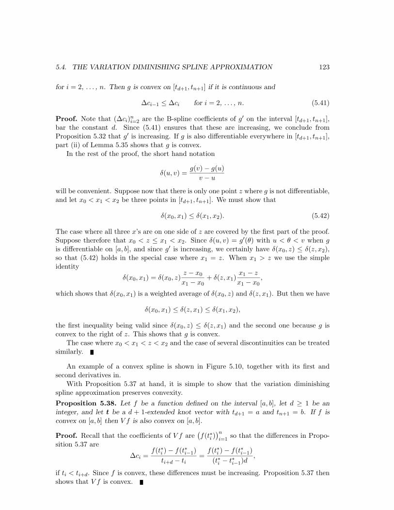
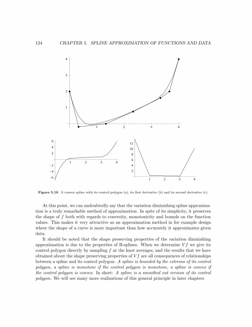
An example of a convex spline is shown in Figure 5.10, together with its first andsecond derivatives in.

With Proposition 5.37 at hand, it is simple to show that the variation diminishingspline approximation preserves convexity.Proposition 5.38. Let f be a function defined on the interval [a, b], let d ≥ 1 be aninteger, and let t be a d + 1-extended knot vector with td+1 = a and tn+1 = b. If f isconvex on [a, b] then V f is also convex on [a, b].

Proof. Recall that the coefficients of V f are(f(t∗i )

)n

i=1so that the differences in Propo-

sition 5.37 are

∆ci =f(t∗i )− f(t∗i−1)

ti+d − ti=

f(t∗i )− f(t∗i−1)(t∗i − t∗i−1)d

,

if ti < ti+d. Since f is convex, these differences must be increasing. Proposition 5.37 thenshows that V f is convex.


1 2 3 4

1

2

3

4

1 2 3 4

-6

-4

-2

2

4

6

1 2 3 4

2

4

6

8

10

12

Figure 5.10. A convex spline with its control polygon (a), its first derivative (b) and its second derivative (c).

At this point, we can undoubtedly say that the variation diminishing spline approxima-tion is a truly remarkable method of approximation. In spite of its simplicity, it preservesthe shape of f both with regards to convexity, monotonicity and bounds on the functionvalues. This makes it very attractive as an approximation method in for example designwhere the shape of a curve is more important than how accurately it approximates givendata.

It should be noted that the shape preserving properties of the variation diminishingapproximation is due to the properties of B-splines. When we determine V f we give itscontrol polygon directly by sampling f at the knot averages, and the results that we haveobtained about the shape preserving properties of V f are all consequences of relationshipsbetween a spline and its control polygon: A spline is bounded by the extrema of its controlpolygon, a spline is monotone if the control polygon is monotone, a spline is convex ifthe control polygon is convex. In short: A spline is a smoothed out version of its controlpolygon. We will see many more realizations of this general principle in later chapters

Documents

Spline Approximation of Functions and Datafolk.uio.no/in329/nchap5.pdf · 100 CHAPTER 5. SPLINE APPROXIMATION OF FUNCTIONS AND DATA 5.1.2 Cubic Hermite interpolation The piecewise