Approximation via Correlation Decay when Strong SpatialMixing Fails∗

Ivona BezákovᆠAndreas Galanis‡ Leslie Ann Goldberg‡ Heng Guo§

Daniel Štefankovič¶

23 January 2019

AbstractApproximate counting via correlation decay is the core algorithmic technique used in

the sharp delineation of the computational phase transition that arises in the approxima-tion of the partition function of anti-ferromagnetic two-spin models.

Previous analyses of correlation-decay algorithms implicitly depended on the occur-rence of strong spatial mixing. This, roughly, means that one uses worst-case analysis ofthe recursive procedure that creates the sub-instances. In this paper, we develop a newanalysis method that is more refined than the worst-case analysis. We take the shapeof instances in the computation tree into consideration and we amortise against certain“bad” instances that are created as the recursion proceeds. This enables us to showcorrelation decay and to obtain an FPTAS even when strong spatial mixing fails.

We apply our technique to the problem of approximately counting independent setsin hypergraphs with degree upper-bound ∆ and with a lower bound k on the arity ofhyperedges. Liu and Lin gave an FPTAS for k ≥ 2 and ∆ ≤ 5 (lack of strong spatialmixing was the obstacle preventing this algorithm from being generalised to ∆ = 6). Ourtechnique gives a tight result for ∆ = 6, showing that there is an FPTAS for k ≥ 3 and∆ ≤ 6. The best previously-known approximation scheme for ∆ = 6 is the Markov-chainsimulation based FPRAS of Bordewich, Dyer and Karpinski, which only works for k ≥ 8.

Our technique also applies for larger values of k, giving an FPTAS for k ≥ ∆. Thisbound is not substantially stronger than existing randomised results in the literature.Nevertheless, it gives the first deterministic approximation scheme in this regime. More-over, unlike existing results, it leads to an FPTAS for counting dominating sets in regulargraphs with sufficiently large degree.

We further demonstrate that in the hypergraph independent set model, approximatingthe partition function is NP-hard even within the uniqueness regime. Also, approximately

∗This work was done in part while the authors were visiting the Simons Institute for the Theory of Com-puting.

†Department of Computer Science, Rochester Institute of Technology, Rochester, NY, USA. Research sup-ported by NSF grant CCF-1319987.

‡Department of Computer Science, University of Oxford, Wolfson Building, Parks Road, Oxford, OX1 3QD,UK. The research leading to these results has received funding from the European Research Council underthe European Union’s Seventh Framework Programme (FP7/2007-2013) ERC grant agreement no. 334828.The paper reflects only the authors’ views and not the views of the ERC or the European Commission. TheEuropean Union is not liable for any use that may be made of the information contained therein.

§School of Informatics, University of Edinburgh, Informatics Forum, Edinburgh, EH8 9AB, UK.¶Department of Computer Science, University of Rochester, Rochester, NY 14627. Research supported by

NSF grant CCF-1563757.

1

counting dominating sets of bounded-degree graphs (without the regularity restriction) isNP-hard.

1 IntroductionWe develop a new method for analysing correlation decays in spin systems. In particular, wetake the shape of instances in the computation tree into consideration and we amortise againstcertain “bad” instances that are created as the recursion proceeds. This enables us to showcorrelation decay and to obtain an FPTAS even when strong spatial mixing fails. To the bestof our knowledge, strong spatial mixing is a requirement for all previous correlation-decaybased algorithms. To illustrate our technique, we focus on the computational complexityof approximately counting independent sets in hypergraphs, or equivalently on counting thesatisfying assignments of monotone CNF formulas.

The problem of counting independent sets in graphs (denoted #IS) is extensively studied.A beautiful connection has been established, showing that approximately counting indepen-dent sets in graphs of maximum degree ∆ undergoes a computational transition which coin-cides with the uniqueness phase transition from statistical physics on the infinite ∆-regulartree. The computational transition can be described as follows. Weitz [22] designed an FP-TAS for counting independent sets on graphs with maximum degree at most ∆ = 5. On theother hand, Sly [19] proved that there is no FPRAS for approximately counting independentsets on graphs with maximum degree at most ∆ = 6 (unless NP = RP). The same connectionhas been established in the more general context of approximating the partition function ofthe hard-core model [22, 16, 19, 4, 6, 20] and in the even broader context of approximating thepartition functions of generic antiferromagnetic 2-spin models [18, 6, 20, 11] (which includes,for example, the antiferromagnetic Ising model). As a consequence, the boundary for theexistence of efficient approximation algorithms for these models has been mapped out1.

Approximate counting via correlation decay is the core technique in the algorithmic devel-opments which enabled the sharp delineation of the computational phase transition. Anotherstandard approach for approximate counting, namely Markov chain Monte Carlo (MCMC)simulation, is also conjectured to work up to the uniqueness threshold, but the current analy-sis tools that we have do not seem to be powerful enough to show that. For example, samplingindependent sets via MCMC simulation is known to have fast mixing only for graphs withdegree at most 4 [14, 3], rather than obtaining the true threshold of 5.

In this work, we consider counting independent sets in hypergraphs with upper-boundedvertex degree, and lower-bounded hyperedge size. A hypergraph H = (V,F) consists of avertex set V and a set F of hyperedges, each of which is a subset of V . A hypergraph is saidto be k-uniform if every hyperedge contains exactly k vertices. Thus, a 2-uniform hypergraphis the same as a graph. We will consider the more general case where each hyperedge hasarity at least k, rather than exactly k.

An independent set in a hypergraph H is a subset of vertices that does not contain ahyperedge as a subset. We will be interested in computing ZH , which is the total numberof independent sets in H (also referred to as the partition function of H). Formally, theproblem of counting independent sets has two parameters — a degree upper bound ∆ and a

1Note that there are non-monotonic examples of antiferromagnetic 2-spin systems where the boundary ismore complicated because the uniqueness threshold fails to be monotonic in ∆ [10]. However, this can becleared up by stating the uniqueness condition as uniqueness for all d ≤ ∆. See [10, 11] for details.

2

lower bound k on the arity of hyperedges. The problem is defined as follows.2

Name #HyperIndSet(k,∆).Instance A hypergraph H with maximum degree at most ∆ where each hyperedge has car-

dinality (arity) at least k.Output The number ZH of independent sets in H.

Previously, #HyperIndSet(k,∆) has been studied using the MCMC technique by Border-wich, Dyer, and Karpinski [1, 2] (see also [3]). They give an FPRAS for all k ≥ ∆ + 2 ≥ 5and for k ≥ 2 and ∆ = 3. Despite equipping path coupling with optimized metrics obtainedusing linear programming, these bounds are not tight for small k. Liu and Lu [12] showedthat there exists an FPTAS for all k ≥ 2 and ∆ ≤ 5 using the correlation decay technique.

Thus, the situation seems to be similar to the graph case — given the analysis toolsthat we have, correlation-decay brings us closer to the truth than the best-tuned analysis ofMCMC simulation algorithms. On the other hand, the technique of Liu and Lu [12] does notextend beyond ∆ = 5. To explain the reason why it does not, we need to briefly describethe correlation-decay-based algorithm framework introduced by Weitz [22]. The main idea isto build a recursive procedure for computing the marginal probability that any given vertexis in the independent set. The recursion works by examining sub-instances with “boundaryconditions” which require certain vertices to be in, or out, of the independent set. The recur-sion structure is called a “computation tree”. Nodes of the tree correspond to intermediateinstances, and boundary conditions are different in different branches. The computation treeallows one to compute the marginal probability exactly but the time needed to do so may beexponentially large since, in general, the tree is exponentially large. Typically, an approx-imate marginal probability is obtained by truncating the computation tree to logarithmicdepth so that the (approximation) algorithm runs in polynomial time. If the correlation be-tween boundary conditions at the leaves of the (truncated) computation tree and the marginalprobability at the root decays exponentially with respect to the depth, then the error incurredfrom the truncation is small and the algorithm succeeds in obtaining a close approximation.

All previous instantiations under this framework require a property called strong spatialmixing (SSM)3, which roughly states that, conditioned on any boundary condition on inter-mediate nodes, the correlation decays. In other words, SSM guards against the worst-caseboundary conditions that might be created by the recursive procedure.

Let the (∆ − 1)-ary k-uniform hypertree Tk,∆ be the recursively-defined hypergraph inwhich each vertex has ∆− 1 “descending” hyperedges, each containing k − 1 new vertices.

Observation 1. Let k ≥ 2. For ∆ ≥ 6, strong spatial mixing does not hold on Tk,∆.

Observation 1 follows from the fact that the infinite (∆−1)-ary tree T2,∆ can be embeddedin the hypertree Tk,∆, and from well-known facts about the phase transition on T2,∆.

Observation 1 prevents the generalisation of Liu and Lu’s algorithm [12] so that it appliesfor ∆ ≥ 6, even with an edge-size lower bound k. The problem is that the constructionof the computation tree involves constructing intermediate instances in which the arity ofa hyperedge can be as small as 2. So, even if we start with a k-uniform hypergraph, the

2Equivalently, one may think of this problem as the problem of counting satisfying assignments of a mono-tone CNF formulas, where vertices are variables and hyperedges are clauses. Being out of the independent set(as a vertex) corresponds to being true (as a variable).

3See Section 2.1 for a definition.

3

computation tree will contain instances with small hyperedges. Without strong spatial mixing,these small hyperedges cause problems in the analysis. Lu, Yang and Zhang [13] discuss thisproblem and say “How to avoid this effect is a major open question whose solution may haveapplications in many other problems.” This question motivates our work.

To overcome this difficulty, we introduce a new amortisation technique in the analysis.Since lack of correlation decay is caused primarily by the presence of small-arity hyperedgeswithin the intermediate instances, we keep track of such hyperedges. Thus, we track notonly the correlation, but also combinatorial properties of the intermediate instances in thecomputation tree. Using this idea, we obtain the following result.

Theorem 2. There is an FPTAS for #HyperIndSet(3, 6).

Note that #HyperIndSet(2, 6) is NP-hard to approximate due to [19], so our result is tightfor ∆ = 6. This also shows that ∆ = 6 is the first case where the complexity of approximatelycounting independent sets differs on hypergraphs and graphs, as for ∆ ≤ 5 both admit anFPTAS [12]. Moreover, Theorem 2 is stronger than the best MCMC algorithm [2] when∆ = 6 as [2] only works for k ≥ 8.

We also apply our technique to large k.

Theorem 3. Let k and ∆ be two integers such that k ≥ ∆ and ∆ ≥ 200. Then there is anFPTAS for the problem #HyperIndSet(k,∆).

In the large k case, our result is not substantially stronger than that obtained by analysisof the MCMC algorithm [2] (k ≥ ∆ rather than k ≥ ∆ + 2) but it is incomparable sinceour algorithm is deterministic rather than randomised. Perhaps more importantly, the boundk ≥ ∆ allows us to connect the problem of counting independent sets in hypergraphs withthe problem of counting dominating sets in ∆-regular graphs and show that the latter admitsan FPTAS when ∆ is sufficiently large. Recall that a dominating set in a graph G is a subsetS of the vertices such that every vertex not in S is adjacent to at least one vertex in S. Wethen consider the following problem.

Name #RegDomSet(∆).Instance A ∆-regular graph G.Output The number of dominating sets in G.

Our theorems have the following corollary.

Corollary 4. For all positive integers ∆ satisfying either ∆ ≤ 5 or ∆ ≥ 199, there is anFPTAS for the problem #RegDomSet(∆).

We remark that Corollary 4 cannot be obtained using the result of [2], i.e., the seeminglysmall difference between k ≥ ∆ and k ≥ ∆ + 2 does matter in deriving Corollary 4 fromTheorems 2 and 3. We should also emphasise that it is necessary to consider ∆-regulargraphs as inputs to the dominating set problem, since otherwise for graphs of maximumdegree ∆ (not necessarily regular), we show that the problem is NP-hard to approximatefor ∆ ≥ 18 (Theorem 52). It is relevant to remark here that we believe that Corollary 4should hold for all ∆; to do this, it would be sufficient to remove the restriction ∆ ≥ 200from Theorem 3. Note that, while we do not know how to remove the restriction, it would atleast be possible to improve “200” to some smaller number. However, we have chosen to stick

4

with “200” in order to keep the proof accessible. We explain next the difficulties in obtainingTheorems 2 and 3.

The main technical difficulty in correlation-decay analysis is bounding a function thatwe call the “decay rate”. This boils down to solving an optimisation problem with (k −1)(∆−1) variables. In previous work (e.g. [17]), this optimisation has been solved using a so-called “symmetrization” argument, which reduces the problem to a univariate optimisation viaconvexity. However, the many variables represent different branches in the computation tree.Since our analysis takes the shape of intermediate instances in the tree into consideration, thesymmetrization argument does not work for us, and different branches take different valuesat the maximum. This problem is compounded by the fact that the shape of the sub-treeconsisting of “bad” intermediate instances is heavily lopsided, and the assignment of variablesachieving the maximum is far from uniform. Given these problems, there does not seem tobe a clean solution to the optimisation in our analysis. Instead of optimizing, we give anupper bound on the maximum decay rate. In Theorem 2, as k and ∆ are small, the numberof variables is manageable, and our bounds are much sharper than those in Theorem 3. Onthe other hand, because of this, the proof of Theorem 3 is much more accessible, and we willuse Theorem 3 as a running example to demonstrate our technique.

We also provide some insight on the hardness side. Recall that for graphs it is NP-hard toapproximate #IS beyond the uniqueness threshold (∆ = 6) [19].4 We prove that it is NP-hardto approximate #HyperIndSet(6, 22) (Corollary 50). In contrast, we show that uniquenessholds on the 6-uniform ∆-regular hypertree iff ∆ ≤ 28 (Corollary 59). Thus, efficient ap-proximation schemes cease to exist well below the uniqueness threshold on the hypertree. Infact, we show that this discrepancy grows exponentially in k: for large k, it is NP-hard toapproximate #HyperIndSet(k,∆) when ∆ ≥ 5 · 2k/2 (Theorem 49 and Corollary 51), despitethe fact that uniqueness holds on the hypertree for all ∆ ≤ 2k/(2k) (Lemma 60). Theorem 49follows from a rather standard reduction to the hard-core model on graphs. Nevertheless, itdemonstrates that the computational-threshold phenomena in the hypergraph case (k > 2)are substantially different from those in the graph case (k = 2).

As mentioned earlier, there are models where efficient (randomised) approximation schemesexist (based on MCMC simulation) even though SSM does not hold. In fact, this can happeneven when uniqueness does not hold. A striking example is the ferromagnetic Ising model(with external field). As [18] shows, there are parameter regimes where uniqueness holdsbut strong spatial mixing fails. It is easy to modify the parameters so that even uniquenessfails. Nevertheless, Jerrum and Sinclair [9] gave an MCMC-based FPRAS that applies for allparameters and for general graphs (with no degree bounds). It is still an open question togive a correlation decay based FPTAS for the ferromagnetic Ising model.

1.1 Note added in revision — recent workAfter our work, Hermon, Sly, and Zhang [8] have shown that the Glauber dynamics forsampling independent sets on n-vertex k-uniform hypergraphs has mixing time O(n log n),if ∆ ≤ c2k/2 for some constant c. Combined with our hardness result, Corollary 51, thisestablishes a sharp computational complexity phase transition, up to constants. Moreover,Moitra [15] has given a deterministic algorithm for approximately counting and samplingthe satisfying assignments of k-CNF formulas, provided that the variable degree ∆ ≲ 2k/60.

4For graphs the uniqueness and SSM thresholds coincide, but for hypergraphs they differ.

5

Moitra’s work relies on connections to the Lovász local lemma. His work improves our ∆ ≤ kbound in Theorem 3 and removes the monotonicity assumption. Despite this recent progress,Theorem 2 remains the best algorithmic result for k = 3.

1.2 Outline of PaperIn Section 2, we first give some preliminaries. We give a formal definition of strong spatialmixing (Section 2.1) and a reformulation of #HyperIndSet(k,∆) as the problem of countingsatisfying assignments in monotone CNF formulas (Section 2.2). This will allow us to use thecomputation tree used by Liu and Lu [12]. A formal description of the computation tree of[12] is given in Section 2.3.

In Section 3, we give an overview of our proof approach, i.e., the main idea behind ournew amortisation technique. Section 3.2 concludes the proof of Theorems 2 and 3, using two(not yet proved) technical lemmas (Lemma 21 and 22) which solve a complicated multivariateoptimisation problem, and represent the bulk of the technical work of the paper. Section 3.3gives the proof of Corollary 4.

In Section 4, we give the proof of Lemma 21, which applies to the large-∆ setting ofTheorem 3 and is by far the technically simpler of the two lemmas. Section 5 contains theproof of the technically more challenging Lemma 22 which applies to the k = 3,∆ = 6 settingof Theorem 2.

Section 6 gives the formal statements and proofs of the hardness results stated in theIntroduction; Section 6.1 has the hardness results for independent sets in hypergraphs andSection 6.2 has the hardness results for dominating sets in graphs. Also, Section 7 studiesthe uniqueness threshold on the k-uniform ∆-regular hypertree (and gives the proofs of theuniqueness statements made in the Introduction). Finally, Section 8 gives the proof for severaltechnical inequalities used in Section 5.

Throughout the paper we use computer algebra to prove multivariate polynomial inequal-ities over the field of real numbers (the coefficients of the polynomials are rational). Morespecifically, we use the Resolve command in Mathematica. The underlying quantifier elim-ination algorithm (described in [21]) provides a rigorous decision procedure that determinesfeasibility of a collection of polynomial inequalities.

2 Preliminaries2.1 Strong Spatial MixingFor the purposes of this section, it will be convenient to view the independent set model as a2-spin model. Namely, if H = (V,F) is a hypergraph, each independent set I can be viewedas a 0, 1-assignment σ to the vertices in V , where a vertex v is assigned the spin 1 under σif v ∈ I and 0 otherwise.

We denote by ΩH the set of all independent sets in H. The Gibbs distribution µH(·) isthe uniform distribution over ΩH . The Gibbs distribution of H can clearly be viewed as theuniform distribution over those assignments σ : V → 0, 1 which encode a valid independentset of H. For an assignment σ : V → 0, 1 and a subset Λ ⊂ V , we denote by σΛ therestriction of σ to the subset Λ.

For a hypergraph H = (V,F) and a subset Λ ⊂ V , we denote by HΛ the subgraph of Hinduced by Λ, i.e., HΛ := (Λ,

∪e∈F (e ∩ Λ)). Also, for a vertex v ∈ V and Λ ⊂ V , we denote

6

by dist(v,Λ) the length of the shortest path5 between v and a vertex of Λ.

Definition 5. Let δ : Z+ → [0, 1]. The independent set model exhibits strong spatial mixingon a hypergraph H = (V,F) with decay rate δ(·) iff for every v ∈ V , for every Λ ⊂ V , for anytwo configurations η, η′ : Λ → 0, 1 encoding independent sets of HΛ, it holds that∣∣∣µH(σ(v) = 1 | σΛ = η)− µH(σ(v) = 1 | σΛ = η′)

∣∣∣ ≤ δ(dist(v,Λ′)

),

where Λ′ denotes the set of vertices in Λ such that η and η′ differ.

2.2 Reformulation in terms of Monotone CNF formulasThe problem of counting the independent sets of a hypergraph has an equivalent formulationin terms of monotone CNF formulas. In order to describe the equivalent formulation, we firstdescribe the problem of counting satisfying assignments of monotone CNF formulas.

A monotone CNF formula C consists of a set of variables V and a set of clauses c1, c2, . . ..Each clause ci is associated with some subset Si of V and is the disjunction of all variablesin Si. The arity of a clause ci, denoted |ci|, is defined to be |Si|. For a variable x ∈ V , itsdegree dx(C) is the number of clauses where x appears. The maximum degree of C is givenby maxx∈V dx(C).

Definition 6. Let Ck,∆ be the set of all monotone CNF formulas which have maximum degreeat most ∆ and whose clauses have arity at least k.

Note that a formula in Ck,∆ may have some clauses with arbitrarily large arities. Asatisfying assignment of the formula is an assignment of truth values to the variables whichmakes the formula evaluate to “true”.

Suppose that H = (V,F) is a hypergraph with maximum degree at most ∆ where eachhyperedge has arity at least k. Let C be the corresponding formula in Ck,∆ with variable set V .The correspondence is that each hyperedge Si of H is associated with exactly one clause ciof C. Independent sets of H are in one-to-one correspondence with satisfying assignmentsof C — a variable is assigned value “true” in an assignment if and only if it is out of thecorresponding independent set.

Going the other direction, any monotone CNF formula can be viewed as a hypergraph.In the technical sections of this paper, we use the monotone CNF formulation.

In this article, when we consider a monotone CNF formula C we will typically use n todenote |V |. Variables in V will be denoted by x1, x2, . . . When x and C are clear from context,we will sometimes use d to denote dx(C). When C is clear from context, we will sometimesuse ∆ to denote maxx∈V dx(C).

2.3 The Computation TreeIn this section, we set up relevant notation and give an exposition of the computation tree ofLiu and Lu [12] which will also be used in our proof (though our analysis will be different).The computation tree of Liu and Lu is given in terms of the monotone CNF version of theproblem. Below we give the relevant definitions and notation; our notation aligns as much aspossible with that of [12].

5A path in a hypergraph with hyperedge set F is a sequence of edges e0, . . . , eℓ ∈ F such that ei ∩ ei+1 = ∅for all i = 0, . . . , ℓ− 1.

7

Our goal is to approximately count the number of satisfying assignments of a formulaC ∈ Ck,∆, which we denote by Z(C). Since C is monotone, an assignment σ : V → 0, 1 issatisfying if, for every clause in C, there is at least one variable x ∈ c with σ(x) = 1. Note thatZ(C) > 0 since the all-1 assignment satisfies every monotone CNF formula. For convenience,we will use the simplified notation “x = 1” to denote (the set of) satisfying assignments ofC in which x is set to 1, and we similarly use “x = 0”. We associate the formula C witha probability distribution in which each satisfying assignment has probability mass 1/Z(C).We will denote probabilities with respect to this distribution by PrC(·).

Let x be a variable in V . Define R(C, x) := PrC(x=0)PrC(x=1) , this is well-defined since PrC(x =

1) > 0 by the monotonicity of C. In fact, the monotonicity of C also implies that 0 ≤R(C, x) ≤ 1, where the upper bound follows from the fact that, for every satisfying assignmentwith x = 0, flipping the assignment of x to 1 does not affect satisfiability. Our interest in thequantity R(C, x) stems from the following simple lemma from [12].

Lemma 7 ([12]). Let k and ∆ be positive integers. Suppose that there is a polynomial-timealgorithm (in n and 1/ε) that takes an n-variable formula C ∈ Ck,∆, a variable x of C, andan ε > 0 and computes a quantity R(C, x) satisfying |R(C, x)−R(C, x)| ≤ ε. Then, there isan FPTAS which approximates Z(C) for every C ∈ Ck,∆.

Proof. The proof is actually identical to the argument in [12, Appendix A]. We include theproof for completeness, and also because an examination of the proof is necessary to checkthat the FPTAS for approximating Z(C) invokes the algorithm that computes R(C, x) onlyon formulas C whose clauses have arity at least k (and maximum degree ∆).

Let ε > 0 and C be a monotone CNF formula C with maximum degree ∆ whose clauseshave arity at least k. Let x1, . . . , xn be the variables in C. Let Ci be the formula obtainedfrom C by setting x1 = · · · = xi = 1 and removing all the clauses that are satisfied (i.e., allclauses that contain a variable from x1, . . . , xi). We have

1

Z(C)= PrC(x1 = . . . = xn = 1) =

n−1∏i=0

PrC(xi+1 = 1 | x1 = · · · = xi = 1)

=n−1∏i=0

PrCi(xi+1 = 1) =n−1∏i=0

1

1 +R(Ci, xi+1).

(1)

Note that every Ci is a monotone CNF formula with maximum degree ∆ whose clauses havearity at least k. By the assumption in the lemma, we can compute (in poly(n, 1/ε) time)quantities R(Ci, xi+1) such that∣∣R(Ci, xi+1)−R(Ci, xi+1)

∣∣ ≤ ε/(100n) for all i = 0, . . . , n− 1. (2)

Let

Z(C) =

n−1∏i=0

(1 + R(Ci, xi+1)

). (3)

It is not hard to conclude from (1), (2) and (3) that (1−ε)Z(C) ≤ Z(C) ≤ (1+ε)Z(C). Thiscompletes the proof.

Liu and Lu [12] established that a computation tree approach gives a recursive procedurefor exactly calculating R(C, x) for any monotone CNF formula C and any variable x ∈ C.

8

We next give the details of this recursive procedure (see [12, Lemma 5]). First, we introducethe following definitions.

Definition 8. Let C be a monotone CNF formula and let x be a variable in C. We call thevariable x forced (in C) if x appears in a clause of arity 1 in C (note that in every satisfyingassignment of C it must be the case that x = 1 and hence R(C, x) = 0). We call the variablex free if x does not appear in any clause of C (note that R(C, x) = 1 in this case).

Definition 9. Let C be a monotone CNF formula and let c be a clause in C. We call theclause c redundant (in C) if there is a clause c′ in C such that c is a (strict) superset of c′(note that removing c from C does not affect the set of satisfying assignments of C).

We next give the details of the computation tree. The nodes in the computation tree willbe pairs (C, x) such that

C is a monotone CNF formula and x is a variable which is not forced in C. (4)

Let (C, x) satisfy (4). We first perform a pre-processing step on C which involves (i) initiallyremoving all of the redundant clauses, (ii) then, removing all clauses of arity 1. Note thatpart (ii) of the preprocessing step removes all forced variables that were present in C; at thetime of the removal, forced variables appear only in clauses of arity 1 since part (i) of thepreprocessing step has already removed all redundant clauses in C (and hence all clauses ofarity greater than 1 that contain forced variables). Denote the formula after the completionof the preprocessing step by C. Note that every clause in C is also a clause in the initialformula C. It follows that x is not forced in C. Further, since removing redundant clausesdoes not change the set of satisfying assignments of C and x is not forced in C, we have thatR(C, x) = R(C, x).

If x is free in C (the formula after the pre-processing step), then the start node (C, x) is(declared) a leaf of the computation tree (note that in this case R(C, x) = 1). In the sequel,we assume that x is not free in C. Denote by cii∈[d] the clauses where x occurs in C andlet wi = |ci| − 1 (note that d ≥ 1). We will use w to denote the vector (w1, . . . , wd). Thevariables in clause ci other than x will be denoted by xi,1, . . . , xi,wi . For the pair (C, x), wenext construct pairs (Ci,j , xi,j) for i ∈ [d] and j ∈ [wi], where Ci,j is an appropriate subformulaobtained from C, roughly, by hard-coding (some of) the occurrences of the variables in C toeither 1 or 0 (this will be explained below and will henceforth be referred to as pinning)6.

Precisely, for i ∈ [d], let Ci be the formula obtained from C by removing clauses c1, . . . , ci−1

(note that this has the same effect as pinning the occurrences of x in these clauses to 1) andpinning the occurrences of x in ci+1, . . . , cd to 0 (this corresponds to removing x from theseclauses, and thus reducing their arities). For j ∈ [wi], the formula Ci,j is obtained from Ciby further removing clause ci and pinning all the occurrences of xi,1, . . . , xi,j−1 to 0.

Before proceeding, let us argue that the pairs (Ci,j , xi,j) satisfy (4) for all i ∈ [d] andj ∈ [wi]. For such i, j, we first prove that Ci,j is a (satisfiable) monotone CNF formula.That is, we prove that the various pinnings in the construction of Ci,j from C do not pin allvariables of some clause of C to 0. For the sake of contradiction, assume otherwise. Observethat Ci,j is obtained from C by either removing some clauses or by pinning some occurrencesof the variables to 0. Clearly, removal of clauses does not affect satisfiability, so we may focuson the effect of pinning. For i ∈ [d] and j ∈ [wi], the only variables whose (some of the)

6Note that our notation for i, j is different from the one in [12]; there, the roles of i, j are interchanged.

9

occurrences in C get pinned to 0 are x, xi,1, . . . , xi,j−1. Since we assumed (for contradiction)that Ci,j is unsatisfiable, it must be the case that there exists a clause c′ in C all of whosevariables are (a subset of) x, xi,1, . . . , xi,j−1. It follows that ci is redundant in C since it isa strict superset of clause c′. This gives a contradiction, since the pre-processing operationensures that C has no redundant clauses. Thus, Ci,j is satisfiable as wanted. Next, we showthat xi,j is not forced in Ci,j . First, observe that xi,j is not forced in C since the secondpart of the preprocessing step ensures that C does not contain forced variables. Thus, theonly way that xi,j can be forced in Ci,j is if there existed a clause c′ in C whose variableswere xi,j together with a subset of x, xi,1, . . . , xi,j−1. Since C includes ci and C does not haveredundant clauses, it must be the case that c′ = ci. It remains to observe that Ci,j does notinclude (any subclause of) ci, from which it follows that xi,j is not forced in Ci,j .

We are now ready to state the relation between R(C, x) and the quantities R(Ci,j , xi,j)with i ∈ [d] and j ∈ [wi].Lemma 10 ([12, Lemma 5]). It holds that

R(C, x) =

d∏i=1

(1−

wi∏j=1

R(Ci,j , xi,j)

1 +R(Ci,j , xi,j)

). (5)

Proof. The proof is identical to the proof of [12, Lemma 5] (which in turn builds on thetechnique of [22]), we give the proof for completeness.

Recall that C is the formula after the preprocessing step and that R(C, x) = R(C, x). Wemay assume that x is not free in C (otherwise, it holds that R(C, x) = 1, which coincides withthe evaluation of the right hand side of (5) under the standard convention that the emptyproduct evaluates to 1).

Equation (5) follows immediately from the following two equalities.

R(C, x) =∏i∈[d]

R(Ci, x), R(Ci, x) = 1−wi∏j=1

R(Ci,j , xi,j)

1 +R(Ci,j , xi,j). (6)

The first equality in (6) is a consequence of a telescoping expansion of PrC(x=0)

PrC(x=1) . To see this,

let C ′ be the formula obtained from C by replacing, for all i ∈ [d], the occurrence of thevariable x in clause ci by a new variable x′i. We have that

R(C, x) =Pr

C(x = 0)

PrC(x = 1)

=Pr

C′(x′1 = 0, . . . , x′d = 0)

PrC′(x

′1 = 1, . . . , x′d = 1)

=∏i∈[d]

PrC′(x

′1 = 1, . . . , x′i−1 = 1, x′i = 0, . . . x′d = 0)

PrC′(x

′1 = 1, . . . , x′i = 1, x′i+1 = 0, . . . x′d = 0)

=∏i∈[d]

PrCi(x = 0)

PrCi(x = 1),

which yields the first equality in (6) after substituting R(Ci, x) =PrCi

(x=0)

PrCi(x=1) .

For the second equality in (6), observe that x appears only in clause ci of the formula Ci,and thus (denoting by Ci\ci the formula which is obtained from Ci by deleting clause ci)

R(Ci, x) =PrCi(x = 0)

PrCi(x = 1)= 1− PrCi\ci(xi,1 = 0, . . . , xi,wi = 0) = 1−

wi∏j=1

PrCi,j (xi,j = 0),

which proves the desired equality after substituting PrCi,j (xi,j = 0) =R(Ci,j ,xi,j)

1+R(Ci,j ,xi,j).

10

By applying (5) recursively, it is not hard to see that one can compute the quantity R(C, x)exactly. Of course, exact computation using this scheme will typically require exponentialtime, so as in [12] we will stop the recursion at some (small) depth L to keep the computationsfeasible within polynomial time. This will yield a quantity R(C, x, L) and the hope is that,by choosing L appropriately, the error |R(C, x, L)−R(C, x)| will be sufficiently small.

In light of (5), a natural way to define R(C, x, L) for integer L ≥ 0 is as follows7.

R(C, x, L) =

1, if x is free in C or L = 0,∏di=1

(1−

∏wij=1

R(Ci,j ,xi,j ,L−1)1+R(Ci,j ,xi,j ,L−1)

), otherwise.

It is immediate that when the formula C has maximum degree bounded by a constant and,further, every clause has arity also bounded above by a constant, one can compute R(C, x, L)in time polynomial in n whenever L = O(log n). To account for formulas where the arities ofthe clauses can be arbitrarily large (but still where the degrees of variables are bounded by aconstant), one needs to be more careful with clauses of large arity (i.e., when their arity as afunction of n is ω(1), say log n). As in [12], we will account for this more general setting bypruning the recursion earlier whenever we encounter clauses with large arity.

Definition 11. For any integer w, let lw := ⌈log6(w + 1)⌉.

Note that l1 = . . . = l5 = 1. For integer L, we set

R(C, x, L) =

1, if x is free in C or L ≤ 0,∏di=1

(1−

∏wij=1

R(Ci,j ,xi,j ,L−lwi )

1+R(Ci,j ,xi,j ,L−lwi )

), otherwise.

(7)

The particular choice of the logarithm base in Definition 11 is not very important aslong as it is a big enough constant. The quantity R(C, x, L) is typically called a “message”(because it gets passed up the computation tree).

Remark 12. For formulas C with a variable x which is not forced in C, we have thelower bound R(C, x) ≥ (1/2)dx(C). The bound is simple to see using (5) and the fact thatR(Ci,j , xi,j) ≤ 1 for all i ∈ [dx(C)] and j ∈ [wi]. Similarly, for all integers L and all nodes(C, x) in the computation tree we have the bound R(C, x, L) ≥ (1/2)dx(C).

3 Proof OutlineWe want to guarantee that the error |R(C, x, L)−R(C, x)| is exponentially small in L. Noticethat if we run the recursion long enough, it computes the true value; namely, R(C, x,∞) =R(C, x). More precisely, we will prove the following two lemmas, which correspond to thesettings of Theorem 2 and Theorem 3, respectively. Recall that Ck,∆ is the set of all monotoneCNF formulas which have maximum degree at most ∆ and whose clauses have arity at least k.Our proof will use the following constant.

Definition 13. Let α = 1− 10−4.7Note that the value 1 of R(C, x, L) when L ≤ 0 is somewhat arbitrary since L ≤ 0 corresponds to stopping

the recursion. Our choice of the value 1 will be convenient for technical reasons that will become apparent inthe proof of the upcoming Lemma 20.

11

Lemma 14. There exists a constant τ > 0 such that for every C ∈ C3,6, every variable x ∈ C,and every integer L,

|R(C, x, L)−R(C, x,∞)| ≤ ταL.

Lemma 15. Let k and ∆ be two integers such that k ≥ ∆ and ∆ ≥ 200. There exists aconstant τ > 0 such that for every C ∈ Ck,∆, every variable x in C, and every integer L,

|R(C, x, L)−R(C, x,∞)| ≤ ταL.

Our proof uses correlation decay techniques together with a new method which accountsfor the shape of the computation tree. Lemma 15 is technically simpler and is proved inSection 4 to better illustrate the idea. Lemma 14 is proved in Section 5. In the rest of thissection, we give an overview of our overall proof strategy.

To analyze the error of the recursion, the standard approach so far in the literature hasbeen to show that, for a node (C, x) in the computation tree, the quantity |R(C, x, L) −R(C, x,∞)| is bounded by αmaxi,j |R(Ci,j , xi,j , L − 1) − R(Ci,j , xi,j ,∞)| for some constant0 < α < 1. This allows one to inductively deduce that |R(C, x, L) − R(C, x,∞)| decaysexponentially in L. This approach has been extremely successful when strong spatial mixingholds [18, 11, 12, 17, 23, 13].

In fact, this step-wise decay seldom holds if we track R(C, x, L) directly. Instead, theanalysis is usually done by tracking Φ(R(C, x, L)) for an appropriate potential function Φ. Inparticular, let Φ : (0, 1] → R be a potential function that satisfies:

Φ is continuously differentiable on (0, 1], and φ := Φ′ satisfies φ(z) > 0 for z ∈ (0, 1]. (8)

The usual approach is to show that |Φ(R(C, x, L))− Φ(R(C, x,∞))| decays exponentially inL, which is sufficient to imply lemmas like Lemma 14 and Lemma 15.

In our setting, this inductive approach is problematic since, inside the computation tree,we are faced with the possibility that the formula at the root of a subtree could have manyarity-2 clauses. For ∆ ≥ 6, these subtrees prohibit the application of the above proof schemesince they are in non-uniqueness and hence the desired step-by-step decay is no longer present,regardless of the choice of the potential function.

While arity-2 clauses are problematic, clauses with larger arities do at least lead to gooddecay of correlation in a single step. In general, as the arity gets larger, the decay gets better.Thus, our approach is to do an amortised analysis. In a single step, we track both the one-stepdecay of correlation and the number of variables in the current formula that are pinned to 0.These 0 pinnings will decrease the effective arity of clauses, and will later lead to worse decay.

More formally, we will track a specific quantity m(C, x, L) which is assigned to each nodein the computation tree. Let C∗ be the original monotone CNF formula and let (C, x) be anode in the computation tree. As explained in Section 2.3, each clause c′ of C is obtainedfrom a clause c of C∗ by pinning a certain number of variables to 0 (possibly none), whicheffectively is the same as removing those variables from the clause. We call these 0-pinningsdeficits and let max0, k − |c′| be the number of deficits of c′. Note that a clause of aritylarger than k is considered to have no deficit, although some variables of it may have beenpinned to 0.

Definition 16. Let D(C) =∑

c′∈C max0, k − |c′| denote the sum of the deficits of theclauses in C.

12

Observe that if a clause c of C∗ does not show up in C, it does not contribute any deficits.For any node (C, x) in the computation tree, let

m(C, x, L) := δD(C)Φ(R(C, x, L))

where δ ∈ (0, 1) is a constant that we will choose later, and the potential function Φ will bespecified shortly in Definition 17. Crucially, the root formula C∗ satisfies

|m(C∗, x, L)−m(C∗, x,∞)| = |Φ(R(C∗, x, L))− Φ(R(C∗, x,∞))|,

since at the root no variable is pinned yet and D(C∗) = 0. Thus, the key step is to show thatthe quantity |m(C, x, L)−m(C, x,∞)| decays exponentially with L; we will show that, for anarbitrary node (C, x) in the computation tree, it holds that

|m(C, x, L)−m(C, x,∞)| ≤ αmaxi,j |m(Ci,j , xi,j , L− 1)−m(Ci,j , xi,j ,∞)|, (9)

where α = 1− 10−4 is from Definition 13.In previous applications of the correlation decay technique, the ordering of the children

of each node (C, x) is usually arbitrary. Since we want to take the shape of the computationtree into consideration, this ordering becomes important to us. We will order clauses in theorder of increasing size, except that we leave arity 2 clauses to the end.

Unfortunately, the quantitym(C, x, L) is more complicated than the plain messageR(C, x, L)and it is even more complicated than Φ(R(C, x, L)), since it incorporates combinatorial infor-mation about the formula C and thus it does not satisfy a simple recursion (unlike R(C, x, L)).Nevertheless, we are able to define a multi-variable quantity κ∗ (see (12)) and we will show(see Lemma 20) that when κ∗ ≤ 1, inequality (9) holds.

We will use the following potential function, which satisfies (8) as required. In general,the choice of an appropriate potential function is guided by an “educated guess”.

Definition 17. Let χ = 1/2 and ψ = 13/10. Define

Φ(z) :=1

χψlog

(zχ

ψ − zχ

).

Let φ(z) denote Φ′(z) so that

φ(z) := Φ′(z) =1

z(ψ − zχ).

Remark 18. The exact values of χ and ψ do not matter at this stage, but it is importantthat 0 < χ ≤ 1 and ψ > 1. For such values of χ and ψ, Φ−1 exists and is uniquely definedover the range of Φ(z) for z ∈ (0, 1].

3.1 A general framework to bound the errorFirst let us calculate how the number of deficits changes in one step of the recursion. Toavoid trivialities, we assume k ≥ 2. Let (C, x) be a node in the computation tree. As inSection 2.3, we first perform a pre-processing step on C which removes redundant clausesand removes clauses of arity 1, producing a new formula C. Every clause in C is a clauseof C, so D(C) ≤ D(C). Also, x is neither forced nor free in C (otherwise, (C, x) is a leaf in

13

the computation tree). Let d = dx(C) and let c1, . . . , cd be the clauses where x occurs in C.Recall that wi = |ci| − 1. As we mentioned in Section 3, the order of c1, . . . , cd is important.We will order clauses in order of increasing size, except that we leave arity-2 clauses to theend. Here is some notation to describe the ordering. Let bℓ denote the number of clausesamongst c1, . . . , cd with arity ℓ. We will use the variables b′ℓ to denote cumulative sums forℓ > 2, so b′2 = 0 and, for ℓ ≥ 3, b′ℓ = b′ℓ−1 + bℓ. We order the clauses so that, for ℓ ≥ 3, clausescb′ℓ−1+1, . . . , cb′ℓ have arity ℓ. Finally, clauses cd−b2+1, . . . , cd have arity 2. Let si be the sumof the deficits of clauses c1, . . . , ci. Thus,

si =

i∑t=1

max(0, k − wt − 1).

We will now consider how the deficits change when we construct the node (Ci,j , xi,j) from(C, x) according to the method described in Section 2.3, where j ∈ [wi].

• The arity-2 clauses in C are always removed in the construction of Ci,j , resulting in aloss of deficit of b2(k − 2).

• The clauses c1, . . . , ci are also removed in the construction of Ci,j resulting in an ad-ditional loss of deficit of smin(i,d−b2). (The minimum is to avoid double-counting ifi > d− b2 since in that cases some of these clauses have arity 2, and have already beencounted.)

• The occurrences of x are pinned to 0 in clauses ci+1, . . . , cd. Consider some t ∈ i +1, . . . , d. If the arity of ct is greater than k then this pinning does not cause anyincrease in deficit. Also, if the arity of ct is 2, then the clause will be removed, so thereis no increase in deficit. Thus, the increase in deficit from these pinnings is at mostmax(0, b′k − i).

• If i ≤ d− b2 then wi > 1 and all occurrences of xi,1, . . . , xi,j−1 are pinned to 0, resultingin an increase in deficit of at most (j − 1)(∆− 1).

Let 1i≤d−b2 be zero-one indicator variable for the event that i is at most d−b2. Then, puttingthese observations together, we conclude that

D(Ci,j) ≤ D(C)− b2(k − 2)− smin(i,d−b2) +max(0, b′k − i) + (j − 1)(∆− 1)1i≤d−b2 .

Since D(C) ≤ D(C), we have

D(Ci,j) ≤ D(C)− b2(k − 2)− smin(i,d−b2) +max(0, b′k − i) + (j − 1)(∆− 1)1i≤d−b2 . (10)

Recall that the recursion for R(C, x, L) depends on the function F d,w(r) implicitly definedby (7), i.e.,

F d,w(r) :=d∏i=1

(1−

wi∏j=1

ri,j1 + ri,j

), (11)

where ri,j ∈ [0, 1] for all i ∈ [d] and j ∈ [wi]. In particular, unless x is free in C or L ≤ 0, wehave

R(C, x, L) = F d,w(R(Ci,j , xi,j , L− lwi)).

14

The m(C, x, L) variables also satisfy a recursion which could be made explicit by map-ping them back to the R(C, x, L) variables, though we will not directly analyse this recur-sion. Instead, we will define a quantity κd,w∗ (r) which tracks the rate at which |m(C, x, L)−m(C, x,∞)| decays in the recursion. Specifically, define κd,w∗ (r) as follows.

κd,w∗ (r) :=

d∑i=1

wi∑j=1

α−lwi δ(b2(k−2)+smin(i,d−b2)−max(0,b′k−i)−(j−1)(∆−1)1i≤d−b2

)φ(Fd,w(r))

φ(ri,j)

∣∣∣∣∂F d,w(r)∂ri,j

∣∣∣∣ .(12)

The main step in the proofs of Lemma 14 and Lemma 15 will be to bound κd,w∗ (r). Byconstruction, the elements in w are in increasing order, apart from the 1s at the end, and thebound on κd,w∗ (r) will use this fact, so we give the following definition.

Definition 19. Let w0 = 2. A vector w = w1, . . . , wd is suitable if its entries are positiveintegers and there is a t ∈ 0, . . . , d such for all j in 1, . . . , t, wj ≥ wj−1 and for all jin t + 1, . . . , d, wj = 1. Given a suitable vector w we use the following global notation(which depends implicitly on w): bℓ is the number of entries of w which are equal to ℓ − 1.b′k = b3 + · · ·+ bk. Finally, si =

∑it=1max(0, k − wt − 1).

Lemma 20. Suppose that ∆ and k are integers with ∆ ≥ 2 and k ≥ 3. Suppose that thereare constants 0 < δ < 1 and U > 0 such that, for all 1 ≤ d ≤ ∆, all suitable w = w1, . . . , wd,and all r satisfying (1/2)∆−11 ≤ r ≤ 1, it holds that

κd,w∗ (r) ≤

1, when d ≤ ∆− 1,

U, when d = ∆.(13)

Then there exists a constant τ > 0 such that, for every C ∈ Ck,∆, every variable x ∈ C,and every integer L, it holds that

|R(C, x, L)−R(C, x,∞)| ≤ ταL. (14)

Proof. We will show that there is a constant τ > 0 such that for all such C, x and L, it holdsthat

|m(C, x, L)−m(C, x,∞)| ≤ ταL. (15)

Assuming (15) for the moment, let us conclude (14). Consider C ∈ Ck,∆. We may assumethat L > 0 since for L = 0 the inequality (14) holds for all sufficiently large τ (any τ ≥ 1works). Consider any x ∈ C and consider the computation tree rooted at (C, x). By thedefinition of m(·, ·, ·) and since by assumption D(C) = 0, we have that

|m(C, x, L)−m(C, x,∞)| =∣∣Φ(R(C, x, L))− Φ(R(C, x,∞))

∣∣. (16)

Let η = (1/2)∆−1 and let

KminΦ := min

x∈[η,1]Φ′(x) = min

x∈[η,1]φ(x), and Kmax

Φ := maxx∈[η,1]

Φ′(x) = maxx∈[η,1]

φ(x).

Since φ is continuous and φ(x) > 0 for all x ∈ [η, 1], we have that KminΦ and Kmax

Φ are positive.We have that

|R(C, x, L)−R(C, x,∞)| ≤ 1

KminΦ

|Φ(R(C, x, L))− Φ(R(C, x,∞))|. (17)

15

To see (17), we may assume that R(C, x, L) = R(C, x,∞) (otherwise the inequality holds atequality), in which case the inequality follows by an immediate application of the Mean ValueTheorem to the function Φ. Combining (16), (17) with (15) yields (14) with τ = τ /Kmin

Φ , asdesired.

To prove (15), we will first show a slightly weaker claim. Namely, for all nodes (C, x) inthe computation tree where C ∈ Ck,∆ and x ∈ C is a variable with degree ≤ ∆ − 1, for allinteger L, it holds that

|m(C, x, L)−m(C, x,∞)| ≤ KmaxΦ αL. (18)

For L ≤ 0, we have that

|m(C, x, L)−m(C, x,∞)| = δD(C)|Φ(R(C, x, L))− Φ(R(C, x,∞))|≤ Kmax

Φ |R(C, x, L)−R(C, x,∞)| ≤ KmaxΦ ,

where in the first inequality we used that δ ∈ (0, 1], D(C) ≥ 0 and an application of theMean Value theorem analogous to the one used in (17), while in the second inequality weused that for L ≤ 0 it holds that R(C, x, L) = 1 (by definition) and 0 ≤ R(C, x,∞) ≤ 1.Since 0 < α < 1, this proves (18) for L ≤ 0.

To prove (18) for integer L > 0 we proceed by induction on L. Namely, we assume thatL > 0 and that (18) holds for all smaller values than L (the base cases L ≤ 0 have alreadybeen shown).

Recall from (4) that x is not forced in C and that C is the formula obtained by removingthe redundant clauses in C. We may assume that x is not free in C — otherwise, observethat R(C, x, L) = R(C, x,∞) = 1 and thus m(C, x, L) = m(C, x,∞), so that (18) holds. Wewill thus focus on x which appear only in (a non-zero number of) clauses in C of arity ≥ 2.Let d = dx(C). For i ∈ [d] and j ∈ [wi], it holds that

m(Ci,j , xi,j , L− lwi) = δD(Ci,j)Φ(R(Ci,j , xi,j , L− lwi))

m(Ci,j , xi,j ,∞) = δD(Ci,j)Φ(R(Ci,j , xi,j ,∞)).(19)

Denote by r(1) the vector whose coordinates are given by R(Ci,j , xi,j , L− lwi) for i ∈ [d] andj ∈ [wi]. Denote also by r(2) the vector whose coordinates are given by R(Ci,j , xi,j ,∞) fori ∈ [d] and j ∈ [wi]. Observe that

R(C, x, L) = R(C, x, L) = F d,w(r(1))

and R(C, x,∞) = R(C, x,∞) = F d,w(r(2)).

Note also that η1 ≤ r(1), r(2) ≤ 1 (cf. property (4) for the nodes of the computation tree, (7),footnote 7 and Remark 12).

We next bound∣∣Φ(F d,w(r(1)))−Φ

(F d,w(r(2))

)∣∣ in terms of maxi,j∣∣Φ(r(1)i,j )−Φ

(r(2)i,j

)∣∣. Forconvenience, denote F := F d,w and for i ∈ [d] and j ∈ [wi], let

z(1)i,j := Φ

(r(1)i,j

), z

(2)i,j := Φ

(r(2)i,j

).

For θ ∈ [0, 1], let zi,j(θ) := θ z(1)i,j + (1 − θ) z

(2)i,j and let ri,j(θ) := Φ−1(zi,j(θ)) (note that

the inverse Φ−1 exists and is uniquely defined in the interval Φ([η, 1]) cf. Remark 18 and (8)).Denote by r(θ) the vector whose coordinates are ri,j(θ) and note that η1 ≤ r(θ) ≤ 1. Finally,let h(θ) := Φ(F (r(θ))). Observe that h is differentiable for all values of θ ∈ [0, 1]. By applying

16

the Mean Value theorem to the function h(θ), we obtain that there exists θ0 ∈ (0, 1) suchthat

Φ(F(r(1)))

− Φ(F(r(2)))

=∂h

∂θ

∣∣∣∣θ=θ0

.

We have that

∂h

∂θ=∂Φ(F (r(θ)))

∂θ= Φ′(F (r(θ)))

∂F (r(θ))

∂θ= Φ′(F (r(θ)))

d∑i=1

wi∑j=1

∂F (r(θ))

∂ri,j

∂ri,j(θ)

∂θ

= Φ′(F (r(θ)))

d∑i=1

wi∑j=1

1

Φ′(ri,j(θ))

∂F (r(θ))

∂ri,j

∂zi,j(θ)

∂θ

= Φ′(F (r(θ)))

d∑i=1

wi∑j=1

1

Φ′(ri,j(θ))

∂F (r(θ))

∂ri,j

(z(1)i,j − z

(2)i,j

) .

It follows that

|m(C, x, L)−m(C, x,∞)|= δD(C)|Φ(R(C, x, L))− Φ(R(C, x,∞))|

≤ maxr

δD(C)

d∑i=1

wi∑j=1

φ(F (r))

φ(ri,j)

∣∣∣∂F (r)∂ri,j

∣∣∣ ∣∣z(1)i,j − z(2)i,j

∣∣= max

r

d∑i=1

wi∑j=1

δD(C)−D(Ci,j)φ(F (r))

φ(ri,j)

∣∣∣∂F (r)∂ri,j

∣∣∣ ∣∣m(Ci,j , xi,j , L− lwi)−m(Ci,j , xi,j ,∞)∣∣ ,

(20)

where the inequality follows by the triangle inequality and the fact (see Definition 17) thatφ = Φ′ satisfies (8). Now note that for all i ∈ [d] and j ∈ [wi], we have by induction that∣∣m(Ci,j , xi,j , L− lwi)−m(Ci,j , xi,j ,∞)

∣∣ ≤ KmaxΦ αL−lwi . (21)

From (20) and the bounds (21), we obtain

|m(C, x, L)−m(C, x,∞)| ≤ KmaxΦ max

r

d∑i=1

wi∑j=1

δD(C)−D(Ci,j)φ(F (r))

φ(ri,j)

∣∣∣∂F (r)∂ri,j

∣∣∣α−lwi

αL.

(22)The lower bounds on D(C)−D(Ci,j), (10), imply that

d∑i=1

wi∑j=1

δD(C)−D(Ci,j)φ(F (r))

φ(ri,j)

∣∣∣∂F (r)∂ri,j

∣∣∣α−lwi ≤ κd,w∗ (r), (23)

where in the inequality we used that δ ∈ (0, 1].Combining (22), (23) and the assumption (13) that κd,w∗ (r) ≤ 1 for d ≤ ∆− 1 yields (18),

as wanted.

17

Finally, we prove (15) with τ := KmaxΦ ·maxU, 1, where U is the constant in assumption

(13). For x of degree ≤ ∆− 1, we get (15) immediately from (18). Now suppose that (C, x)are such that x has degree ∆ in C. Note, for a node (C ′, x′) in the computation tree, x′ mayhave degree d = ∆ in C ′ only if (C ′, x′) is the root of the tree. It follows that the childrenof the node (C, x), say (Ci,j , xi,j) with i ∈ [d] and j ∈ [wi], are such that xi,j has degreeat most ∆ − 1 in Ci,j . Hence, by applying (18), we obtain that (21) holds for all i, j andhence (as before) we deduce that (22), (23) hold as well. Inequality (15) now follows since byassumption (13) we have that κd,w∗ (r) ≤ maxU, 1 for d ≤ ∆.

This concludes the proof of Lemma 20.

We now state two technical lemmas which will be proved later in the paper. These lemmasverify the premise of Lemma 20 in the settings of Theorems 2 and 3. Note from Equation (12)that κd,w∗ (r) depends on the global quantity k and on various quantities (depending on w)which are defined in Definition 19.

Lemma 21. Let k and ∆ be two integers such that k ≥ ∆ and ∆ ≥ 200. There are constants0 < δ < 1 and U > 0 such that, for all 1 ≤ d ≤ ∆, all suitable w = w1, . . . , wd, and all rsatisfying 0 < r ≤ 1, it holds that

κd,w∗ (r) ≤

1, when d ≤ ∆− 1,

U, when d = ∆.

Lemma 22. Let ∆ = 6 and k = 3. There are constants 0 < δ < 1 and U > 0 such that, forall 1 ≤ d ≤ ∆, all suitable w = w1, . . . , wd, and all r satisfying (1/2)∆−11 ≤ r ≤ 1, it holdsthat

κd,w∗ (r) ≤

1, when d ≤ ∆− 1,

U, when d = ∆.

Lemma 21 will be proved in Section 4 and Lemma 22 will be proved in Section 5. Usingthese lemmas and Lemma 20, we can prove Lemma 14 and Lemma 15.

Lemma 14. There exists a constant τ > 0 such that for every C ∈ C3,6, every variable x ∈ C,and every integer L,

|R(C, x, L)−R(C, x,∞)| ≤ ταL.

Proof. The lemma follows immediately from Lemma 22 and Lemma 20.

Lemma 15. Let k and ∆ be two integers such that k ≥ ∆ and ∆ ≥ 200. There exists aconstant τ > 0 such that for every C ∈ Ck,∆, every variable x in C, and every integer L,

|R(C, x, L)−R(C, x,∞)| ≤ ταL.

Proof. The lemma follows immediately from Lemma 21 and Lemma 20.

3.2 Proof of the main theoremsIn this section, we give the proofs of Theorems 2 and 3, which we restate here for convenience.

Theorem 2. There is an FPTAS for #HyperIndSet(3, 6).

18

Proof. First, reformulate #HyperIndSet(3, 6) as the monotone CNF problem with instancesin C3,6, following the reformulation in Section 2.2. Then, just invoke Lemmas 7 and 14.

Theorem 3. Let k and ∆ be two integers such that k ≥ ∆ and ∆ ≥ 200. Then there is anFPTAS for the problem #HyperIndSet(k,∆).

Proof. Once again, reformulate #HyperIndSet(k,∆) as the monotone CNF problem with in-stances in Ck,∆. Then invoke Lemmas 7 and 15.

We have now finished the proofs of Theorems 2 and 3 except that we have not yet provedthe Lemmas 21 and 22 which we used to bound κd,w∗ (r) in the proofs of Lemmas 14 and 15.Lemma 21 will be proved in Section 4 and Lemma 22 will be proved in Section 5. The proofsbound the multivariate decay rate function κd,w∗ (r). This is an optimisation problem that isquite complicated to solve. Moreover, we need to solve it for all possible suitable vectors w.The analysis of bounding κd,w∗ (r) is the technical core of our proof.

3.3 Application to counting dominating setsIn this section, we use Theorems 2 and 3 to obtain Corollary 4, which we restate here forconvenience.

Corollary 4. For all positive integers ∆ satisfying either ∆ ≤ 5 or ∆ ≥ 199, there is anFPTAS for the problem #RegDomSet(∆).

The corollary follows from the observation that a dominating set in a ∆-regular graph isdefined by a collection of constraints of arity ∆ + 1 with each variable occurring in ∆ + 1constraints. The details are spelled out in the following proof.

Proof of Corollary 4. Let ∆ be an integer satisfying either 2 ≤ ∆ ≤ 5 or ∆ ≥ 199. Let G bea ∆-regular graph and denote by #DomSets(G) the number of dominating sets in G.

Let k′ := ∆ + 1,∆′ := ∆ + 1. We will construct a k′-uniform hypergraph H where ev-ery vertex of H has degree ∆′ such that the number ZH of independent sets in H satisfiesZH = #DomSets(G). To conclude the corollary we then only have to check that, for therelevant range of ∆, we can invoke one of the FPTASes of Theorems 2 and 3 to approxi-mate ZH . Indeed, when ∆ ≥ 199, we have ∆′ ≥ 200 and k′ ≥ ∆′. Thus, by Theorem 3,#HyperIndSet(k′,∆′) admits an FPTAS and thus so does #RegDomSet(∆). Similarly, when2 ≤ ∆ ≤ 5, we have ∆′ ≤ 6 and k′ ≥ 3. By Theorem 2, #HyperIndSet(3, 6) admits an FPTASand thus so does #RegDomSet(∆).

We conclude the proof by showing the construction of H. For a vertex v ∈ V of G, denoteby v1, . . . , v∆ its neighbours in G (note that there are exactly ∆ of those since G is ∆-regular)and let ev = v, v1, . . . , v∆. Then H is the hypergraph with vertex set V and hyperedge setF = ∪v∈V ev. It is clear from the construction that H is k′-uniform with k′ = ∆+1. Further,every vertex v of H has degree ∆′ = ∆+1 since it appears in the hyperedges ev, ev1 , . . . , ev∆ .This completes the construction of H.

It remains to show that the number of dominating sets in the graph G is equal to thenumber of independent sets in the hypergraph H. It suffices to show that S ⊆ V is anindependent set of H iff V \S is a dominating set of G. Indeed, if S is an independent set ofH, then for every vertex v ∈ S, at least one of v1, . . . , v∆ is not in S (since ev is a hyperedge ofH) and hence V \S is a dominating set of G. Similarly, if V \S is a dominating set of G, then

19

for every vertex v ∈ S, at least one of v1, . . . , v∆ is in V \S and hence S is an independent setof H (since each hyperedge ev of H contains at least one vertex which does not belong to S).

This completes the proof.

4 Bounding the decay rate for large ∆

This section is devoted to proving Lemma 21. Let k and ∆ be two integers such that k ≥ ∆and ∆ ≥ 200. We start by setting up some upper bounds on the function κd,w∗ (r) which isdefined in (12) using notation from Definition 19. Consider the following definitions, whichapply to suitable vectors w.

ρw,i(r) :=

α−lwi δsi+i−d+b2

∑wij=1 δ

−(j−1)(∆−1) 1φ(ri,j)

∣∣∣∂F d,w

∂ri,j

∣∣∣ if 1 ≤ i ≤ d− b2,

α−lwi δsd−b21

φ(ri,1)

∣∣∣∂F d,w

∂ri,1

∣∣∣ if d− b2 + 1 ≤ i ≤ d.. (24)

κd,w(r) := φ(F d,w(r))δb2(k−2)d∑i=1

ρw,i(r). (25)

We first argue that κd,w∗ (r) ≤ κd,w(r). To see this, note that smin(i,d−b2) is si for 1 ≤ i ≤d− b2 and is sd−b2 for d− b2+1 ≤ i ≤ d. Also, b′k ≤ d− b2, so max(0, b′k− i) ≤ d− b2− i and ifi ≥ d− b2+1 then max(0, b′k− i) = 0. Finally, (j−1)(∆−1)1i≤d−b2 is equal to (j−1)(∆−1)when 1 ≤ i ≤ d− b2 and to 0 when d− b2 + 1 ≤ i.

Recall from Definition 13 that α = 1− 10−4. For brevity, we will denote F d,w(r) by F (r).Finally, we define the constant δ (which depends on ∆).

Definition 23. Let c = 0.7. Given ∆, define δ by δ∆ = c.

In order to bound κd,w(r), an important special case is when b2 = 0. Indeed, as we willsee soon, handling this special case implies an upper bound of κd,w(r) for the general case.Define the following quantity for suitable vectors w.

κd,w(r) :=1

ψ − F (r)χ

d∑i=1

δsi+i−d−(wi−1)(∆−1)α−lwi

∏wij=1

ri,j1+ri,j

1−∏wij=1

ri,j1+ri,j

wi∑j=1

ψ − rχi,j1 + ri,j

. (26)

The next lemma gives an upper bound on the quantity κd,w(r).

Lemma 24. Let k and ∆ be two integers such that k ≥ ∆ and ∆ ≥ 200. Let d be a positiveinteger such that d ≤ ∆− 1. Let w = w1, . . . , wd be a suitable vector with b2 = 0. Then, forall r satisfying 0 < r ≤ 1, κd,w(r) ≤ 1.

In the case d = ∆ for w = w1, . . . , wd, a suitable vector with b2 = 0 and all r satisfying0 < r ≤ 1, κd,w(r) ≤ 1/δ.

Note that in the statement of Lemma 24, the wi’s are positive integers in non-decreasingorder, all of which are at least 2. Lemma 24 will be proved in the remainder of Section 4.First we use it to prove Lemma 21, which we restate for convenience.

20

Lemma 21. Let k and ∆ be two integers such that k ≥ ∆ and ∆ ≥ 200. There are constants0 < δ < 1 and U > 0 such that, for all 1 ≤ d ≤ ∆, all suitable w = w1, . . . , wd, and all rsatisfying 0 < r ≤ 1, it holds that

κd,w∗ (r) ≤

1, when d ≤ ∆− 1,

U, when d = ∆.

Proof. First note that ∣∣∣∣ ∂F∂ri,j∣∣∣∣ = F (r)

ri,j(1 + ri,j)·∏wit=1

ri,t1+ri,t

1−∏wit=1

ri,t1+ri,t

.

Hence, for 1 ≤ i ≤ d− b2,

ρw,i(r) = F (r)δsi+i−d+b2α−lwi

∏wij=1

ri,j1+ri,j

1−∏wij=1

ri,j1+ri,j

wi∑j=1

δ−(j−1)(∆−1) 1

φ(ri,j)

1

ri,j(1 + ri,j)

≤ F (r)δsi+i−d+b2−(wi−1)(∆−1)α−lwi

∏wij=1

ri,j1+ri,j

1−∏wij=1

ri,j1+ri,j

wi∑j=1

ψ − rχi,j1 + ri,j

;

and for d− b2 < i ≤ d,

ρw,i(r) =α−l1F (r)

φ(ri,1)δsd−b2

ri,11 + ri,1

≤ F (r)δsd−b2α−l1ri,1(ψ − rχi,1)

1 + ri,1.

Recall from Definition 11 that lwi = ⌈log6(wi + 1)⌉ and in particular that l1 = . . . = l5 = 1.This implies that

κd,w(r) ≤ δb2(k−2)

ψ − F (r)χ

(d−b2∑i=1

δsi+i−d+b2−(wi−1)(∆−1)α−lwi

∏wij=1

ri,j1+ri,j

1−∏wij=1

ri,j1+ri,j

wi∑j=1

ψ − rχi,j1 + ri,j

+

d∑i=d−b2+1

δsd−b2

ri,1(ψ − rχi,1)

α(1 + ri,1)

). (27)

We want to move the term in front of the parentheses in (27) inside. Let w′ = w1, . . . , wd−b2be the prefix of w. Then

F d−b2,w′(r) =

d−b2∏i=1

1−wi∏j=1

ri,j1 + ri,j

.

21

First, suppose that d ≤ ∆− 1. By (27),

κd,w(r) ≤δb2(k−2)

(1

ψ − F d−b2,w′(r)χ

d−b2∑i=1

δsi+i−d+b2−(wi−1)(∆−1)α−lwi

∏wij=1

ri,j1+ri,j

1−∏wij=1

ri,j1+ri,j

wi∑j=1

ψ − rχi,j1 + ri,j

+1

ψ −∏di=d−b2+1(1 + ri,1)−χ

d∑i=d−b2+1

δsd−b2

ri,1(ψ − rχi,1)

α(1 + ri,1)

)

≤δb2(k−2)

κd−b2,w′(r) +

d∑i=d−b2+1

1

ψ − (1 + ri,1)−χ·ri,1(ψ − rχi,1)

α(1 + ri,1)

≤δb2(k−2)

1 +d∑

i=d−b2+1

1

ψ − (1 + ri,1)−χ·ri,1(ψ − rχi,1)

α(1 + ri,1)

, (28)

where we use the definition of κd,w from (26) and Lemma 24 (using the fact that d ≤ ∆− 1)in the last step. In Section 8.1.1, we verify using Mathematica’s Resolve function that, forany 0 ≤ r ≤ 1, it holds that

1

ψ − (1 + r)−χ· r(ψ − rχ)

α(1 + r)≤ 0.42. (29)

Therefore (28) simplifies into

κd,w(r) ≤ δb2(k−2) (1 + 0.42b2) .

Since δk−2 ≤ δ∆−2 ≤ c1−2/200 and c = 0.7, we have that

κd,w∗ (r) ≤ κd,w(r) ≤ 1,

for any integer b2 ≥ 0. This finishes the proof.The bound in the case d = ∆ follows the same argument; the only difference is that in

equation (28) we use the d = ∆ case of Lemma 24 and hence obtain a weaker (constant)bound on κd,w(r).

4.1 Useful lemmas for the proof of Lemma 24We have now finished the proof of Theorem 3 apart from the proof of Lemma 24, and theremainder of Section 4 is devoted to the proof of Lemma 24. First, in this section, we provesome useful lemmas. To make them easier to read, we list some useful constants and functionsin Tables 1 and 2. The first two lemmas are merely technical.

Lemma 25. Let f(r) := ψ−rχ1+r for r ∈ (0, 1] and parameterize t in terms of r via et = r

1+r .Then, f , viewed as a function of t, is concave.

Proof. Note that since r ranges from 0 to 1, we have that t ranges from −∞ to ln(1/2).Further, we have that r = et

1−et , so we want to show that the function

f(t) := f( et

1− et

)is concave for all t ≤ ln(1/2). We do this by verifying that f ′′(t) < 0 for t ≤ ln(1/2) usingMathematica’s Resolve function, see Section 8.1.2 for details.

22

Name Value Definitionα 1− 10−4 Definition 13ψ 13/10 Definition 17χ 1/2 Definition 17c 0.7 Definition 23δ δ = c1/∆ Definition 23c5 c1−6/200 Definition 31K2 1.11614 Lemma 27K6 1 Lemma 27τ2 4.5932 Lemma 29τ6 2.7805 Lemma 29Y0 ≈ 0.933133 (54)Y1 ≈ 0.988369 (54)

Table 1: Constants

Name Defining equationκd,w(r) (26)ξ(w, r) (35)ζ(w, d) (41)h1(y) (53)h(y) (55)σt,6(y) (57)σ8,2(y) (59)

Table 2: Functions

Lemma 26. Let x, y be such that 0 < y < x < 1. For integers d,w ≥ 1, consider the functionsf1(d) :=

1−xd1−yd and f2(w) := 1−xw

1−xw+1 /1−yw

1−yw+1 . Then, for all integer d,w ≥ 1, it holds that

f1(d) ≤ f1(d+ 1), f2(w) ≥ f2(w + 1).

Proof. To show that f1(d) ≤ f1(d + 1) for integer d ≥ 1, we only need to show that f1(y) ≤f1(x) where f1(t) := 1−td+1

1−td , i.e., that f1(t) is increasing for t ∈ (0, 1). We calculate

f1′(t) =

td−1(td+1 − (d+ 1)t+ d

)(1− td)

2 ,

which is nonnegative for all t ∈ (0, 1) since the quantity td+1 − (d+1)t+ d is nonnegative fort ∈ (0, 1) (it vanishes at t = 1 and is a decreasing function in t for t ∈ (0, 1] since the firstderivative equals (d+ 1)(td − 1) ≤ 0).

To show that f2(w) ≥ f2(w+1) for integer w ≥ 1, we only need to show that f2(x) ≤ f2(y)

where f2(t) := (1−tw)(1−tw+2)(1−tw+1)2

, i.e., that f2(t) is decreasing for t ∈ (0, 1). We calculate

f2′(t) =

(1− t)tw−1(wtw+2 − (w + 2)tw+1 + t(w + 2)− w

)(1− tw+1)3

,

which is at most 0 for all t ∈ (0, 1) since the quantity wtw+2 − (w + 2)tw+1 + t(w + 2)−w isat most 0 for t ∈ [0, 1] (it vanishes at t = 1, it is negative at t = 0 and is a concave functionin t for t ∈ [0, 1] since the second derivative equals w(w + 2)(w + 1)(tw − tw−1) ≤ 0).

We now turn to the problem of upper bounding κd,w(r) which is what we need to do toprove Lemma 24. Recall from Definition 19 that si =

∑it=1max(0, k − wt − 1). Thus, for

i ≥ 1 and d ≤ ∆− 1, we have

si + i− d− (wi − 1)(∆− 1) ≥ si + i− wi(∆− 1)

≥ si−1 + k − wi − 1 + i− wi(∆− 1)

≥ si−1 + k − wi∆.

23

Hence, from the definition of κd,w(r), we have

κd,w(r) ≤ δk

ψ − F (r)χ

(d∑i=1

δsi−1−wi∆α−lwi

∏wij=1

ri,j1+ri,j

1−∏wij=1

ri,j1+ri,j

wi∑j=1

ψ − rχi,j1 + ri,j

). (30)

Recall from (11) that F (r) =∏di=1

(1−

∏wij=1

ri,j1+ri,j

). Define ti,j by eti,j = ri,j/(1 + ri,j)

and let ui =∑wi

j=1 ti,j . Then we can express the right-hand-side of (30) as a function of theti,j ’s as follows.

δk

ψ −(∏d

i=1(1− eui))χ(

d∑i=1

δsi−1−wi∆α−lwieui

1− eui

wi∑j=1

f(ti,j)

),

where f is defined in Lemma 25. By Lemma 25, f is concave, so Jensen’s inequality applies,showing that the quantity is at most

δk

ψ −(∏d

i=1(1− eui))χ(

d∑i=1

δsi−1−wi∆α−lwieui

1− euiwif

(uiwi

)).

So we can replace each ti,j with ui/wi without decreasing the right-hand-side. Equivalently,we can replace each ri,j with a quantity ri so that

∏wij=1

ri,j1+ri,j

=(

ri1+ri

)wi

.

Define yi such that yi =(1−

(ri

1+ri

)wi)1/2

. Also notice that δk ≤ δ∆ = c = 0.7. From(30), we thus obtain that :

κd,w(r) ≤ δk

ψ −∏di=1 yi

d∑i=1

δsi−1g(yi, wi), (31)

where

g(y, w) := c−wα−lww1− y2

y2

(1− (1− y2)1/w

)(ψ −

((1− y2)1/w

1− (1− y2)1/w

)χ), (32)

and the range of yi is yi ∈ [(1−2−wi)1/2, 1). The next lemma gives an upper bound on g(y, w).

Lemma 27. For all w ≥ 2, for all y ∈ [(1− 2−w)1/2, 1), it holds that

g(y, w) ≤ Kw g((1− 2−w)1/2, w) = 0.15Kwα−lww(2c)−w

(1− 2−w

)−1, (33)

where K2 = 1.11614, K3 = 1.03, K4 = 1.01, and Kw = 1 for all w ≥ 5. In particular,Kw+1 ≤ Kw for any w ≥ 2.

Proof. The equality in (33) is immediate by just substituting y = (1 − 2−w)1/2 into g(y, w),so we only need to argue for the inequality in (33).

We make the change of variable t = (1 − y2)1/w so that the range of t is (0, 1/2]. Theinequality can then be written as

g(t, w)

g(1/2, w)≤ Kw where g(t, w) := tw

1− tw(1− t)

(ψ −

( t

1− t

)χ). (34)

24

We verify (34) for w = 2, 3, 4, 5 and all t ∈ (0, 1/2] using Mathematica’s Resolve function,see Section 8.1.3 for details. To obtain the lemma for w ≥ 6, it then suffices to show that

g(t, w + 1)

g(1/2, w + 1)≤ g(t, w)

g(1/2, w)for all t ∈ (0, 1/2].

This can be massaged into

g(t) ≤ g(1/2), where g(t) := g(t, w + 1)

g(t, w)=t(1− tw)

1− tw+1,

so it suffices to show that g is increasing for t ∈ (0, 1/2]. We calculate

g′(t) =wtw+1 − (w + 1)tw + 1

(1− tw+1)2,

which is positive for all t ∈ (0, 1) since the function f(t) := wtw+1 − (w + 1)tw + 1 satisfiesf(1) = 0 and f ′(t) = w(w + 1)tw(1− 1

t ) < 0 for all t ∈ (0, 1).

For every positive integer w, define ξ(w, 0) = 0. For every positive integer d, define

ξ(w, d) := α−lw(2c)−ww(1− 2−w

)−1d−1∑i=0

δmax0,k−w−1i. (35)

In order to upper bound κd,w(r) it is going to be useful to know when ξ(w, d) is decreasingin w. This is captured by the following lemma.

Lemma 28. Let k,∆ be integers satisfying k ≥ ∆, ∆ ≥ 200. Then for all integers d suchthat 1 ≤ d ≤ ∆, for all integers w satisfying either 2 ≤ w ≤ k − 3 or w ≥ k − 1, it holds thatξ(w + 1, d) ≤ ξ(w, d).

Proof. Recall from Definition 11 that lw = ⌈log6(w + 1)⌉. Thus, lw − lw+1 ∈ 0,−1. Usingthis fact and the fact that 0 < α < 1, we obtain that

ξ(w + 1, d)

ξ(w, d)= αlw−lw+1(2c)−1(1 + w−1)

1− 2−w

1− 2−w−1

∑d−1i=0 δ

max0,k−w−2i∑d−1i=0 δ

max0,k−w−1i

≤ (2αc)−1(1 + w−1)1− 2−w

1− 2−w−1Dw,d, (36)

whereDw,d :=

∑d−1i=0 δ

max0,k−w−2i∑d−1i=0 δ

max0,k−w−1i,

Note that when w ≥ k − 1, Dw,d is trivially equal to 1, so for this range of w the right handside of (36) is upper bounded by 1 (since w ≥ k − 1 ≥ 199 and, from α = 1 − 10−4 andc = 0.7, we have (2αc)−1 < 3/4).

Henceforth, we will thus focus on the range 2 ≤ w ≤ k− 3. To bound the right-hand sideof (36), we will use the following bound on Dw,d:

Dw,d ≤Mw, where Mw :=

2/(1 + c), if k − 3 ≥ w ≥ 6,

1.05, if 2 ≤ w ≤ 5.(37)

25

We will justify the bound in (37) shortly, for now note that the desired inequality ξ(w +1, d)/ξ(w, d) ≤ 1 will follow from

Mw(2ac)−1(1 + w−1)

1− 2−w

1− 2−w−1≤ 1. (38)

We verify (38) for w = 2, 3, 4, 5 and also show that for w = 6 we have Mw(2ac)−1(1+w−1) < 1

(for w ≥ 7 the result follows by monotonicity), see Section 8.1.4 for the code.We finish the proof by justifying the bound in (37). Note that for all 2 ≤ w ≤ k − 3, we

have thatDw,d =

1− δ(k−w−2)d

1− δ(k−w−1)d· 1− δk−w−1

1− δk−w−2

To prove (37) for 2 ≤ w ≤ 5, we use the fact that k ≥ ∆ ≥ 200, the definition δ∆ = c and thefact that the function x/(1− x) is increasing for x ∈ (0, 1) to obtain

Dw,d ≤1− δk−w−1

1− δk−w−2= 1 +

δk−w−2

1− δk−w−2(1− δ) ≤ 1 +

c1−7/∆

1− c1−7/∆(1− c1/∆)

≤ 1 +c1−7/200

1− c1−7/200(1− c1/200) ≤ 1.05, (39)

see Section 8.1.4 for the calculation in the last inequality. To prove (37) for 6 ≤ w ≤ k − 3,we will show that

Dw,d ≤ Dw,∆ ≤ Dk−3,∆ =1 + δ

1 + c< 2/(1 + c). (40)

To justify (40), note that the equality is immediate using that δ∆ = c. Also, the very last(strict) inequality in (40) is immediate using 0 < δ < 1. In the following, we may thusfocus on proving the first two inequalities in (40). To justify the first inequality in (40), i.e.,Dw,d ≤ Dw,∆ for 1 ≤ d ≤ ∆, just use Lemma 26 for the function f1 with x = δk−w−2 andy = δk−w−1. For the second inequality in (40), i.e., Dw,∆ ≤ Dk−3,∆ for 6 ≤ w ≤ k − 3, notethat, by δ∆ = c,

Dw,∆ =1− c(k−w−2)

1− c(k−w−1)· 1− δk−w−1

1− δk−w−2=

1− cw′

1− cw′+1/

1− δw′

1− δw′+1, where w′ := k − w − 2.

Then Dw,∆ ≤ Dk−3,∆ when w ≤ k − 3 (i.e., w′ ≥ 1) follows from Lemma 26 for the functionf2 with x = δ and y = c.

This concludes the proof of the bound in (37), which completes the proof of Lemma 28.

For w = w1, . . . , wd define the quantity

ζ(w, d) :=d∑i=1

δsi−1α−lwi (2c)−wiwi(1− 2−wi

)−1. (41)

In order to upper bound κd,w(r) it is going to be useful to have an upper bound on ζ(w, d)and this is done in the following lemma.

Lemma 29. Let k,∆ be integers satisfying k ≥ ∆, ∆ ≥ 200. Let τ2 := 4.5932 and τ6 :=2.7805. Consider d ≤ ∆ and let w = w1, . . . , wd be a vector of integers satisfying w1 ≤ · · · ≤wd.

26

1. If w1 ≥ 2 then ζ(w, d) ≤ τ2.

2. If w1 ≥ 6 then ζ(w, d) ≤ τ6.

Proof. We wish to find an upper bound for ζ(w, d). The reason that the task is difficult isthat the vector w may have up to d different entries. We say that a vector w′ = w′

1, . . . , w′d

of integers dominates w if the following are true.

• w′1 = w1,

• w′1 ≤ · · · ≤ w′

d,

• For all i, w′i ≤ wi, and

• ζ(w, d) ≤ ζ(w′, d).

So a good way to find an upper bound for ζ(w, d) is to find a “simple” vector w′ whichdominates w and then find an upper bound for ζ(w′, d). To do this, we define several classesof vectors w, depending on how “desirable” they are for proving upper bounds.

• A vector w of integers is “partly good” if 2 ≤ w1 ≤ · · · ≤ wd.

• A vector w is “fairly good” if it is partly good and w1 = · · · = wd or wd ≤ k − 1.

• A vector w is “very good” if it is fairly good and every wi is in w1, k − 1.

The vector w that we start with (in the statement of the lemma) is partly good, but itwill be easiest to prove upper bounds on ζ(w, d) for very good vectors w. Thus, we will definetwo transformations.

1. The first transformation starts with a partly good vector w. If w is fairly good, thenthe transformation does nothing. Otherwise, it produces a partly good vector w′ = wwhich dominates w.

2. The second transformation starts with a fairly good vector w. If w is very good, thenthe transformation does nothing. Otherwise, it produces a fairly good vector w′ = wwhich dominates w.

Both transformations make progress in the sense that there exists an i such that w′i < wi.

If we start with any partly good vector w and repeatedly apply the first transformationthen, after a finite number of transformations, we must obtain a fairly good vector w′ whichdominates w. (The reason that a finite number of transformations suffices is that eachindividual transformation makes progress, but the entries stay sorted, and the first coordinatenever changes.) Next, we apply the second transformation repeatedly, starting from w′.Again, after a finite number of transformations, we end up with a very good vector w′′ whichdominates w′ and therefore dominates w. An upper bound on ζ(w′′, d) gives an upper boundon ζ(w, d). So to finish the proof, we must show that the two transformations are possible.Then we must show that for every very good vector w with w1 ≥ 2, ζ(w, d) ≤ τ2 and wemust show that for every very good vector w with w1 ≥ 6, ζ(w, d) ≤ τ6.

Transformation 1: Start with a partly good vector w. If w is fairly good, do nothing.Otherwise, wd > max(w1, k − 1). Choose the integer t to be as small as possible, subject

27

to the constraint that, for all i in t + 1, . . . , d, we have wi = wd. Note that 1 ≤ t < d andwt < wd. Recall from Definition 19 that si =

∑ij=1max(0, k−wj−1). Since wt+1 = · · · = wd

we have for any j ∈ 0, . . . , d − t that st+j = st + max0, k − wd − 1j. This means that∑di=t+1 δ

si−1 = δst∑d−t−1

i=0 δmax0,k−wd−1i. So,

ζ(w, d) =

t∑i=1

δsi−1α−lwi (2c)−wiwi(1− 2−wi

)−1+ δstξ(wd, d− t). (42)

By Lemma 28, ξ(wd, d − t) ≤ ξ(max(wt, k − 1), d − t), so decreasing wt+1 = · · · = wd fromwd to max(wt, k − 1) does not decrease ζ(w, d). Thus, the transformation sets w′

t+1 = · · · =w′d = max(wt, k − 1) and, w′

1, . . . , w′t = w1, . . . , wt.

Transformation 2: Start with a fairly good vector w. If w is very good, do nothing.Otherwise, w1 < wd ≤ k − 1. Choose the integer t to be as small as possible, subject to theconstraint that, for all i in t+1, . . . , d, we have wi = k−1. Clearly, t ≤ d. We defined ξ(w, 0)to be 0, so from (42), we have

ζ(w, d) =t∑i=1

δsi−1α−lwi (2c)−wiwi(1− 2−wi

)−1+ δstξ(k − 1, d− t). (43)

Now, choose the integer t′ to be small as possible, subject to the constraint that, for alli ∈ t′ + 1, . . . , t, wi = wt. Since w is not very good, 1 ≤ t′ < t and wt′ < wt < k − 1. Sincewt′+1 = · · · = wt, we can decompose the right-hand side of (43) as

ζ(w, d) =

t′∑i=1

δsi−1α−lwi (2c)−wiwi(1− 2−wi

)−1+ δst′ ξ(wt, t− t′) + δstξ(k − 1, d− t).

Now wt′ < wt < k − 1 implies wt′ ≤ k − 3 and wt ≤ k − 2 so by Lemma 28, ξ(wt, d − t) ≤ξ(wt′ , d − t), so decreasing wt′+1 = · · · = wt from wt to wt′ does not decrease ζ(w, d).Thus, the transformation sets w′

t′+1 = · · · = w′t = wt′ and w′

1, . . . , w′t′ = w1, . . . , wt′ and

w′t+1 = · · · = w′

d = wt+1 = · · · = wd = k − 1.To finish the proof, we must show that for every very good vector w with w1 ≥ 2, ζ(w, d) ≤

τ2 and we must show that for every very good vector w with w1 ≥ 6, ζ(w, d) ≤ τ6. Now ifw is a very good vector, then choose t as small as possible so that wt+1 = · · · = wd = k − 1.Note that 0 ≤ t ≤ d and w1 = · · · = wt and wt+1 = · · · = wd = k − 1. Thus,

ζ(w, d) ≤ ξ(w1, t) + ξ(k − 1, d− t). (44)

To bound the terms in (44), note that ξ(k − 1, 0) = 0 and for any 1 ≤ d − t ≤ ∆ ≤ k itholds that

ξ(k − 1, d− t) = α−lk−1(2c)−(k−1)(k − 1)(1− 2−(k−1)

)−1(d− t) ≤ 2k2(2αc)−(k−1) < 10−10,

(45)where the last inequality follows from (2αc)−1 < 3/4 and k ≥ 200.

For t = 0, we have ξ(w1, t) = 0 and ξ(k− 1, d− t) < 10−10 by (45). Thus assume t > 0 so

28

that w1 < k − 1. Then, by Lemma 28, for k − 1 > w1 ≥ 2, we have ξ(w1, t) ≤ ξ(2, t) and

ξ(2, t) = α−1(2c)−22(1− 2−2

)−1t−1∑i=0

δ(k−3)i.

≤ α−1(2c)−22(1− 2−2

)−1 1

1− δk−3

= α−1(2c)−22(1− 2−2

)−1 1

1− c(k−3)/∆

≤ α−1(2c)−22(1− 2−2

)−1 1

1− c1−3/200. (46)

The numerical calculation in Section 8.1.5 shows that this is at most 4.5931. Since this plus10−10 is less than τ2, we obtain the first part of the lemma. Similarly,

ξ(6, t) ≤ α−2(2c)−66(1− 2−6

)−1 1

1− c1−7/200≤ 2.78045, (47)

see Section 8.1.5 for the calculation in the last inequality. Since 2.78045 + 10−10 < τ6, weobtain the second part of the lemma, and we have finished the proof of the lemma.

4.2 A quick proof of a weaker TheoremOur goal is to prove Lemma 24, but the proof, which will be given in Section 4.3, is a littlebit technical. In order to give the intuition, without getting into technical details, we firststate and prove a weaker version of the lemma. Lemma 30, below, is identical to Lemma 24,except that the condition k ≥ ∆ has been strengthened to k ≥ 2.64∆. Using Lemma 30 inplace of Lemma 24 strengthens the condition to k ≥ 2.64∆ in Lemmas 21 and 15. Thus,Lemma 30 gives immediately a weaker version of Theorem 3 where the condition k ≥ ∆ isreplaced with k ≥ 2.64∆.

Lemma 30. Let k and ∆ be two integers such that k ≥ 2.64∆ and ∆ ≥ 200. Let d be apositive integer such that d ≤ ∆ − 1. Let w = w1, . . . , wd be a suitable vector with b2 = 0.Then, for all r satisfying 0 < r ≤ 1, κd,w(r) ≤ 1.

In the case d = ∆ for w = w1, . . . , wd, a suitable vector with b2 = 0 and all r satisfying0 < r ≤ 1, κd,w(r) ≤ 1/δ.

Proof. Recall that for d ≤ ∆− 1,

κd,w(r) ≤ δk

ψ −∏di=1 yi

d∑i=1

δsi−1g(yi, wi), (31)

where yi =(1−

(ri

1+ri

)wi)1/2

and yi ∈ [(1−2−wi)1/2, 1). From Lemma 27 we have g(yi, wi) ≤0.15K2α

−lwiwi(2c)−wi (1− 2−wi)

−1, so, from the definition of ζ(w, d) (see (41)),

κd,w(r) ≤ δk

ψ − 10.15K2ζ(w, d) ≤

c2.64

ψ − 10.15K2τ2, (48)

where in the last inequality we used the fact that ζ(w, d) ≤ τ2 from the first part of Lemma 29and the fact that δk ≤ δ2.64∆ = c2.64. It is a matter of a simple numerical calculation to check

29

that the right hand side of (48) is less than 1, see Section 8.1.6 for details. Thus, we haveshown that κd,w(r) < 1.

The case d = ∆ has the same proof, the only difference is that in equations (30) and (31)we replace δk by δk−1, losing a factor of 1/δ (the upper bound is valid using the same argumentas before, now using inequality si + i− d− (wi − 1)(∆− 1) ≥ si−1 + (k − 1)− wi∆).

4.3 The Proof of Lemma 24Recall that our actual goal is to prove Lemma 24, which is stronger than Lemma 30 becauseit only assumes k ≥ ∆, not k ≥ 2.64∆. Recall that

κd,w(r) ≤ δk

ψ −∏di=1 yi

d∑i=1

δsi−1g(yi, wi), (31)

where yi =(1−

(ri

1+ri

)wi)1/2

so that yi ∈ [(1− 2−wi)1/2, 1) and the function g(y, w) is givenby (32). Using the fact that k ≥ ∆ and δ∆ = c we obtain the inequality

κd,w(r) ≤ c

ψ −∏di=1 yi

d∑i=1

δsi−1g(yi, wi). (49)

Lemma 27 gives an upper bound on g(y, w) in terms of the constants Kw. Since Kw = 1 forall w ≥ 5, we want to split the sum in (49) for w ≤ 5 and w ≥ 6. More generally, we split thesummation in the bound (49) at an index t ≤ d using Lemma 27 as follows.

κd,w(r) ≤ c

ψ −∏di=1 yi

(t∑i=1

δsi−1g(yi, wi) +d∑

i=t+1

δsi−1g(yi, wi)

)

≤ c

ψ −∏ti=1 yi

(t∑i=1

δsi−1g(yi, wi) + 0.15δstKwt+1

d∑i=t+1

δsi−1−stα−lwi (2c)−wiwi(1− 2−wi

)−1

)

=c

ψ −∏ti=1 yi

(t∑i=1

δsi−1g(yi, wi) + 0.15δstKwt+1

d∑i=t+1

δs′i−1α−lwi (2c)−wiwi

(1− 2−wi

)−1

),

=c

ψ −∏ti=1 yi

(t∑i=1

δsi−1g(yi, wi) + 0.15δstKwt+1ζ(w′, d− t)

), (50)

where s′i−1 = si−1 − st =∑i−1

j=t+1max(0, k − wj − 1), w′ = wt+1, . . . , wd, and the functionζ(w, d) is defined in (41).

Intuitively, the term ζ(w′, d − t) bounds a tail sum coming from the last d − t clausescorresponding to the variables wt+1, . . . , wd. Recall from the statement of Lemma 24 and thesentences following its statement that the wj ’s are in increasing order. Preferably, we wantto choose the index t to split the sum in (50) so that wt ≤ 5 and wt+1 ≥ 6. However, we alsodo not want too many terms to be in the first sum (since each of these will cause us work),so we insist that t ≤ 8. When t = 8, we will use the bound wt+1 ≥ 2. If t < 8 we will be ableto use the stronger bound wt+1 ≥ 6.

30

The first step in the proof of Lemma 24 is to find a good way to control g(y, w) for 2 ≤w ≤ 5. To this end, we use a piecewise linear function to upper bound g(y, w). In particular,in Section 8.1.7, we verify using Mathematica’s Resolve function that, for w = 2, 3, 4, 5 andy ∈ [(1− 2−w)1/2, 1), it holds that

g(y, w) ≤ h1(y), where h1(y) := min0.2279,−1.5y + 1.6276,−8y + 8.052. (51)

Moreover, let t6+1 be the first index where wt6+1 ≥ 6. Therefore wi ≤ 5 for all 2 ≤ i ≤ t6.Then applying (50) with t = t6 and Lemma 29,

κd,w(r) ≤ c

ψ −∏t6i=1 yi

(t6∑i=1

δsi−1g(yi, wi) + 0.15δst6 τ6

)

≤ c

ψ −∏t6i=1 yi

(t6∑i=1

δ(i−1)(k−6)h1(yi) + 0.15δt6(k−6)τ6

), (52)

where, for i ∈ 1, . . . , t6, yi is in the range [(1− 2−wi)1/2, 1). Since each wi is at least 2, wehave (1− 2−wi)1/2 ≥

√3/2, so each yi ∈ [

√3/2, 1].

The function h1(y) is non-increasing, and in fact

h1(y) =

0.2279 if

√3/2 ≤ y ≤ Y0;

−1.5y + 1.6276 if Y0 ≤ y ≤ Y1;

−8y + 8.052 if Y1 ≤ y ≤ 1,

(53)

where Y0 ≈ 0.933133 and Y1 ≈ 0.988369 are two constants such that

−1.5Y0 + 1.6276 = 0.2279,

−1.5Y1 + 1.6276 = −8Y1 + 8.052.(54)

Notice that h1(yi) is a constant for yi ∈ [√3/2, Y0]. Moreover, c

ψ−∏t

i=1 yiis an increasing

function of yi for each i. Hence, to upper bound the right-hand side of (52), we may restrictthe yi’s to be in the interval [Y0, 1]. More precisely, let

h(y) :=

−1.5y + 1.6276 if Y0 ≤ y ≤ Y1;

−8y + 8.052 if Y1 ≤ y ≤ 1.(55)

Definition 31. Let c5 := c1−6/200.

Observe that c5 = δ∆(1−6/200) ≥ δ∆−6 ≥ δk−6 as k ≥ ∆ ≥ 200 and δ < 1. By (52) we havethat

κd,w(r) ≤ c

ψ −∏t6i=1 yi

(t6∑i=1

δ(i−1)(k−6)h(yi) + 0.15ct65 τ6

)

≤ c

ψ −∏t6i=1 yi

(t6∑i=1

ci−15 h(yi) + 0.15ct65 τ6

), (56)

where each yi ∈ [Y0, 1].

31

What is left is to bound the right hand side of (56). For yi ∈ [Y0, 1], define

σt,6(y) :=c

ψ −∏ti=1 yi

(t∑i=1

ci−15 h(yi) + 0.15ct5τ6

), (57)

where τ6 can be found in Table 1. The following lemma, which is proved in Section 4.4,bounds σt,6(y) when 0 ≤ t ≤ 7.

Lemma 32. Let t be an integer such that 0 ≤ t ≤ 7. For any (y1, . . . , yt) where each yi is inthe range [Y0, 1], we have σt,6(y) ≤ 1.

Combining (56), (57) and Lemma 32 we get an upper bound on κd,w(r) provided w issuch that t6 ≤ 7. If t6 ≥ 8, we will set t = 8 in (50). Similarly to deriving (56), we get that

κd,w(r) ≤ c

ψ −∏8i=1 yi

(8∑i=1

ci−15 h(yi) + 0.15c85K2τ2

), (58)

where each yi ∈ [Y0, 1] and K2 and τ2 can be found in Table 1. Similarly to (57), defineσ8,2(y) to be the right-hand side of (58). Namely,

σ8,2(y) :=c

ψ −∏8i=1 yi

(8∑i=1

ci−15 h(yi) + 0.15c85K2τ2

). (59)

The next lemma bounds σ8,2(y) and is proved in Section 4.4.

Lemma 33. For any (y1, . . . , y8) where each yi is in the range [Y0, 1], we have σ8,2(y) ≤ 1.

We can now prove Lemma 24, which we restate here for convenience.

Lemma 24. Let k and ∆ be two integers such that k ≥ ∆ and ∆ ≥ 200. Let d be a positiveinteger such that d ≤ ∆− 1. Let w = w1, . . . , wd be a suitable vector with b2 = 0. Then, forall r satisfying 0 < r ≤ 1, κd,w(r) ≤ 1.

In the case d = ∆ for w = w1, . . . , wd, a suitable vector with b2 = 0 and all r satisfying0 < r ≤ 1, κd,w(r) ≤ 1/δ.

Proof. Consider t6.

1. If t6 ≤ 7, then by (56), (57), and Lemma 32, κd,w(r) ≤ σt6,6(y) ≤ 1.

2. Otherwise t6 ≥ 8. By (58), (59) and Lemma 33, κd,w(r) ≤ σ8,2(y) ≤ 1.

The case d = ∆ has the same proof. Like the proof of Lemma 30, the only differencein the d = ∆ case is that in equations (30) and (31) we replace δk by δk−1, losing a factorof 1/δ (the upper bound is valid using the same argument as before, now using inequalitysi + i− d− (wi − 1)(∆− 1) ≥ si−1 + (k − 1)− wi∆).

32

4.4 Remaining ProofsIn this section we provide technical details of Lemma 32 and Lemma 33, which we restate forconvenience.

Lemma 32. Let t be an integer such that 0 ≤ t ≤ 7. For any (y1, . . . , yt) where each yi is inthe range [Y0, 1], we have σt,6(y) ≤ 1.

Proof. Recall that

σt,6(y) :=c

ψ −∏ti=1 yi

(t∑i=1

ci−15 h(yi) + 0.15ct5τ6

), (57)

where c5 = c1−6/200, c = 0.7 and τ6 = 2.7805 are as in Table 1 and the function h(y) is givenby (55). For t = 0, we have

σ0,6(y) =0.15cτ6ψ − 1

≈ 0.973044 < 1, (60)

see Section 8.1.8 for the calculation. For t = 1, we have

σ1,6(y) =c

ψ − y1

(h(y1) + 0.15c5τ6

)≤ 1, (61)

see Section 8.1.8 for the verification using Mathematica’s Resolve function. Thus, we mayassume that t ≥ 2 henceforth.

For the sake of contradiction, suppose that there exists y′ such that σt,6(y′) > 1 for some2 ≤ t ≤ 7. We will gradually adjust the variables y′i without decreasing σt,6(y′) until there isonly one variable left, in which case we will be able to exclude the possibility that σt,6(y′) > 1.

We first observe that the partial derivative of σt,6(y) with respect to yi is

∂σt,6(y)

∂yi=

1

ψ −∏tj=1 yj

(σt,6(y)

∏tj=1 yj

yi− 1.5cci−1

5

), (62)

if Y0 ≤ yi ≤ Y1, and

∂σt,6(y)

∂yi=

1

ψ −∏tj=1 yj

(σt,6(y)

∏tj=1 yj

yi− 8cci−1

5

), (63)

if Y1 ≤ yi ≤ 1.Suppose that there exists an index 3 ≤ i ≤ t such that y′i ≤ Y1. Using our initial

assumption that σt,6(y′) > 1, we then have (from (62) and y′j ≥ Y0) that

∂σt,6(y)

∂yi

∣∣∣∣y=y′

>1

ψ −∏tj=1 y

′j

(Y t−10 − 1.5cci−1

5

)> 0, (64)

for any 2 ≤ t ≤ 7 and 3 ≤ i ≤ t, see Section 8.1.8 for the verification of the last inequality.Hence σt,6(y) is increasing in this y′i and we may thus assume y′i ≥ Y1 for all 3 ≤ i ≤ t.

33

Suppose that y′2 ≤ Y1. Then, using that y′i ≥ Y1 for all 3 ≤ i ≤ t and y′1 ≥ Y0, togetherwith our assumption that σt,6(y′) > 1, we have (from (62)) that

∂σt,6(y)

∂y2

∣∣∣∣y=y′

>1

ψ −∏tj=1 y

′j

(Y0Y

t−21 − 1.5cc5

)> 0 (65)

for any 2 ≤ t ≤ 7, see Section 8.1.8 for the verification of the last inequality. Arguing asbefore, we may therefore assume y′i ≥ Y1 for all 2 ≤ i ≤ t.

Suppose that there exists an index 2 ≤ i ≤ min5, t such that y′i > Y1. Since y′i ≥ Y1 forall 2 ≤ i ≤ t and y′1 ≥ Y0, we obtain (from (57)) the following upper bound on σt,6(y′) (usingalso the fact that h is decreasing):

σt,6(y′) ≤ c

ψ − 1

(h(Y0) +

t∑i=2

ci−15 h(Y1) + 0.15ct5τ6

). (66)

Plugging (66) into (63) and using the fact that the yj ’s are at most 1, we obtain that

∂σt,6(y)

∂yi

∣∣∣∣y=y′

≤ 1

ψ −∏tj=1 y

′j

(c

ψ − 1

(h(Y0) + c5h(Y1)

1− ct−15

1− c5+ 0.15ct5τ6

)− 8cci−1

5

)< 0,

(67)see Section 8.1.8 for the verification of the last inequality. Therefore σt,6(y) is decreasing in y′ifor any 2 ≤ i ≤ min5, t and we may therefore assume that y′i = Y1 for any 2 ≤ i ≤ min5, t.

For 2 ≤ t ≤ 5, using the fact that y′2 = . . . = y′t = Y1, we thus have that

σt,6(y′) =

c

ψ − y′1Yt−11

(h(y′1) + c5h(Y1)

1− ct−15

1− c5+ 0.15ct5τ6

)> 1, (68)

which is false for all y′1 ∈ [Y0, 1], see Section 8.1.8 for the proof using Mathematica’s Resolvefunction. Similarly, for t = 6, using that y′2 = . . . = y′5 = Y1, Y1 ≤ y′6 ≤ 1 and that h isdecreasing, we have that

1 < σ6,6(y′) ≤ c

ψ − y′1Y41

(h(y′1) + c5h(Y1)

1− c551− c5

+ 0.15c65τ6

), (69)

which is false for all y′1 ∈ [Y0, 1], see Section 8.1.8 for the proof using Mathematica’s Resolvefunction. Finally, for t = 7, we have that y′2 = y′3 = y′4 = y′5 = Y1. Using this andY1 ≤ y′6, y

′7 ≤ 1, we obtain that

1 < σ7,6(y′) ≤ c

ψ − y′1Y41

(h(y′1) + c5h(Y1)

1− c651− c5

+ 0.15c75τ6

), (70)

which is false for all y′1 ∈ [Y0, 1], see Section 8.1.8 for the proof using Mathematica’s Resolvefunction.

Thus, for all 2 ≤ t ≤ 7, the assumption that there exists y′ such that σt,6(y′) > 1 has leadto a contradiction, thus completing the proof of Lemma 32 for all 0 ≤ t ≤ 7.

The proof of Lemma 33 is very similar.

34

Lemma 33. For any (y1, . . . , y8) where each yi is in the range [Y0, 1], we have σ8,2(y) ≤ 1.

Proof. Recall that

σ8,2(y) :=c

ψ −∏8i=1 yi

(8∑i=1

ci−15 h(yi) + 0.15ct5K2τ2

), (59)

where c5 = c1−6/200, c = 0.7, K2 = 1.11614 and τ2 = 2.7805 are as in Table 1 and the functionh(y) is given by (55). For the sake of contradiction, suppose that there exists y′ such thatσ8,2(y

′) > 1. We will gradually adjust the variables y′i without decreasing σ8,2(y′) until thereis only one variable left, in which case we can directly verify that σ8,2(y′) > 1 is impossible.

Identically to Lemma 32, the partial derivative of σ8,2(y) with respect to yi is

∂σ8,2(y)

∂yi=

1

ψ −∏8j=1 yj

(σ8,2(y)

∏8j=1 yj

yi− 1.5cci−1

5

), (62)

if Y0 ≤ yi ≤ Y1, and

∂σ8,2(y)

∂yi=

1

ψ −∏8j=1 yj

(σ8,2(y)

∏8j=1 yj

yi− 8cci−1

5

), (63)

if Y1 ≤ yi ≤ 1. We may thus use the same line of arguments as in Lemma 32 to concludethat we may assume that y′i ≥ Y1 for 3 ≤ i ≤ 8 (by verifying (64) for t = 8 and 3 ≤ i ≤ 8),and then bootstrap that to y′i ≥ Yi for 2 ≤ i ≤ 8 (by verifying (65) for t = 8 and i = 2), seeSection 8.1.9 for the details of the verification.

We thus obtain the following upper bound for σ8,2(y′) (this is an analogue of (66) whichis obtained using the fact that h is decreasing):

σ8,2(y′) ≤ c

ψ − 1

(h(Y0) +

8∑i=2

ci−15 h(Y1) + 0.15c85K2τ2

). (71)

Now suppose that there exists an index 2 ≤ i ≤ 5 such that y′i > Y1. We plug (71) into (63)and obtain the following analogue of (67):

∂σ8,2(y)

∂yi

∣∣∣∣y=y′

≤ 1

ψ −∏8j=1 y

′j

(c

ψ − 1

(h(Y0) + c5h(Y1)

1− c751− c5

+ 0.15c85K2τ2

)− 8cci−1

5

)< 0,

(72)see Section 8.1.9 for the details of the verification of the last inequality. Thus, we may assumethat y′i = Y1 for 2 ≤ i ≤ 5.

Then we can bootstrap our bound on σ8,2(y′) in (71) to

σ8,2(y′) ≤ c

ψ − y′1Y41

(h(y′1) +

8∑i=2

ci−15 h(Y1) + 0.15c85K2τ2

), (73)

which gives that

∂σ8,2(y)

∂y6

∣∣∣∣y=y′

≤ 1

ψ −∏tj=1 y

′j

(cY 4

1

ψ − y′1Y41

(h(y′1) + c5h(Y1)

1− c751− c5

+ 0.15c85K2τ2

)− 8cc55

)< 0.

(74)

35

where the last inequality holds for all y′1 ∈ [Y0, 1], see Section 8.1.9 for the verification usingMathematica’s Resolve function. This implies that we can set y′6 = Y1 as well.

Using y′2 = · · · = y′5 = y′6 = Y1, Y1 ≤ y′7, y′8 ≤ 1 and the fact that h is decreasing, we

obtain that

1 < σ8,2(y′) ≤ c

ψ − y′1Y51

(h(y′1) + c5h(Y1)

1− c751− c5

+ 0.15c85K2τ2

), (75)

which is false for all y′1 ∈ [Y0, 1], see Section 8.1.9 for the proof using Mathematica’s Resolvefunction.

Thus, the assumption that there exists y′ such that σ8,2(y′) > 1 has led to a contradiction.This completes the proof of the lemma.

5 Bounding the decay rate for k = 3, ∆ = 6

In this section, we fix k = 3 and ∆ = 6. This section is devoted to proving Lemma 22, whichwe restate here for convenience.

Lemma 22. Let ∆ = 6 and k = 3. There are constants 0 < δ < 1 and U > 0 such that, forall 1 ≤ d ≤ ∆, all suitable w = w1, . . . , wd, and all r satisfying (1/2)∆−11 ≤ r ≤ 1, it holdsthat

κd,w∗ (r) ≤

1, when d ≤ ∆− 1,

U, when d = ∆.

In the statement of Lemma 22, d is an integer between 1 and 6. The vector w is a suitablevector, which is defined in Definition 19. This means that the entries w1, . . . , wd are in non-decreasing order, except that any “1” entries are left to the end. The definition of “suitable”also includes some global notation which depends implicitly on w: For all positive integers ℓ,bℓ is the number of entries amongst w1, . . . , wd which are equal to ℓ− 1. Hence,

∑∞ℓ=2 bℓ = d.

Also, w1, . . . , wb3 are all equal to 2, whereas for i > b3, wi is either 1 or it is at least 3. Wehave k = 3 so b′3 = b3. Finally, si =

∑it=1max(0, 2 − wt). Recall the definition of κd,w∗ (r)

from (12), which we have specialised here to k = 3:

κd,w∗ (r) :=d∑i=1

wi∑j=1

α−lwi δ(b2+smin(i,d−b2)−max(0,b3−i)−(j−1)(∆−1)1i≤d−b2

)φ(Fd,w(r))

φ(ri,j)

∣∣∣∣∂F d,w∂ri,j

∣∣∣∣ .Consider the following definitions, which apply to all suitable w.

ρw,i(r) := α−lwi

wi∑j=1

(1

δ

)(j−1)(∆−1) 1

φ(ri,j)

∣∣∣∣∂F d,w∂ri,j

∣∣∣∣ . (76)

κd,w(r) := φ(F (r)) δb2( b3∑i=1

(1δ

)b3−iρw,i(r) +

d∑i=b3+1

ρw,i(r)

). (77)

We first argue that κd,w∗ (r) ≤ κd,w(r). To see this, note that smin(i,d−b2) ≥ 0. Also, theterm max(0, b3 − i) is b3 − i if 1 ≤ i ≤ b3 and is 0 if i > b3. Finally, 1i≤d−b2 ≤ 1.

Definition 34. Let δ = 9789/10000.

36

We can now state a lemma which immediately implies Lemma 22 since κd,w∗ (r) ≤ κd,w(r).

Lemma 35. Let ∆ = 6 and k = 3. There is constant U > 0 such that, for all 1 ≤ d ≤ ∆, allsuitable w = w1, . . . , wd, and all r satisfying (1/2)∆−11 ≤ r ≤ 1, it holds that

κd,w(r) ≤

1, when d ≤ ∆− 1,

U, when d = ∆.

The rest of the section contains the proof of Lemma 35. This is a more involved optimi-sation problem than the one that arose in the proof of Lemma 21. Before delving into thedetails, we set up some convenient notation and then give a roadmap of the argument.

5.1 Outline of the proofFor convenience, let F := F d,w, κ(r) := κd,w(r) which is defined in (77) and for i ∈ [d],let ρi(r) := ρw,i(r) which is defined in (76). Our goal is to show that, for all r such that

12∆−11 ≤ r ≤ 1, it holds that κ(r) ≤ 1 when d ≤ ∆−1 and that κ(r) is bounded by a constantwhen d = ∆.

Here is a rough outline of our analysis.

1. The first part of the proof will be to bound the quantities ρi(r) appropriately for eachi ∈ [d]. Namely, the main goal here will be to replace the ri,jj∈[wi] by a suitablequantity ri. In fact, for this part of the proof, rather than working with the ri,j ’s, itwill be easier to work with ti,j =

ri,j1+ri,j

See Lemma 36.

2. After the first part, we will have reduced significantly the dimensionality of the optimi-sation problem: from the initial number of

∑i∈[d]wi variables ri,ji∈[d],j∈[wi], we will

be left with just d “representative” variables (one for each i).

3. Despite having reduced the number of variables quite a lot, the wi’s so far can bearbitrarily large integers. It will be convenient for us to restrict the range of the wi’s.Using a rather crude argument, we will be able to restrict our attention to i’s such that1 ≤ wi ≤ 5. Intuitively, the reason is that large wi’s make κ smaller. We quantify thiseffect in an appropriate way for our analysis. (See Lemma 37.)

4. The next step is a further reduction of the number of variables. In particular, recallfrom Item 2 that we have reduced to the case where the number of variables is d (one foreach i) and, from Item 3, for each i ∈ [d] it holds that 1 ≤ wi ≤ 5. We will further grouptogether these variables according to their values. That is, for integer 1 ≤ w ≤ 5 we willbe able to use a single variable (indexed by w) to capture the aggregate contribution ofthe variables wi with wi = w. (See Equation (98) and the inequality in Lemma 40 andthe relevant Lemmas 39 and 40.)

5. At this point, we are able to do the final steps of the optimisation. The most importantcase turns out to be when all of the wi’s are either 1 or 2 (Lemma 41). In this case, weobtain quite sharp bounds for κ for each value of d (i.e, d = 1, 2, . . . ,∆− 1 = 5). Thisfacilitates the application of cruder arguments to handle the cases where there existi ∈ [d] with wi = 1, 2 (Lemmas 42, 43 and 44).

37

5.2 The details of the argumentIn this section, we expand in detail the outline of Section 5.1 and give the necessary technicalingredients needed to complete the proof of Lemma 35. Later subsections contain the left-overtechnical proofs which would significantly interrupt the flow.

The first part of the proof will be to bound the quantities ρi(r) appropriately. For i ∈ [d]and j ∈ [wi], we have (by differentiating lnF (r) as in the proof of Lemma 21):

∂F

∂ri,j= −F (r)

∏wij′=1

ri,j′1+ri,j′

1−∏wij′=1

ri,j′1+ri,j′

1

ri,j(1 + ri,j).

Let g(z) := 1φ(z)

1z(1+z) =

ψ−zχ1+z . For i ∈ [d], the quantity ρi(r) can then be written as

ρi(r) := F (r)

∏wij=1

ri,j1+ri,j

1−∏wij=1

ri,j1+ri,j

α−lwi

wi∑j=1

(1δ

)(j−1)(∆−1)g(ri,j). (78)

Let ti,j := ri,j1+ri,j

and let ti be the geometric mean of the ti,j ’s, i.e., (ti)wi :=∏wij=1 ti,j =∏wi

j=1ri,j

1+ri,j. As we shall see soon, ti will be used to capture the “aggregate” effect of wi.

Let t be the vector whose entries are given by ti,j with i ∈ [d] and j ∈ [wi]. Note that1

2∆−1+11 ≤ t ≤ (1/2)1.

We will view the quantities κ(r) and ρi(r) as a function of t. For that, it will be convenientto consider the function

h(t) := g

(t

1− t

)= (1− t)

[ψ −

(t

1− t

)χ](79)

for t ∈ [1/(2∆−1 + 1), 1/2]. With this preprocessing, for i ∈ [d], the quantities ρi(r), κ(r) asa function of t become

ρi(t) = F (t)(ti)

wi

1− (ti)wiα−lwi

wi∑j=1

(1δ

)(j−1)(∆−1)h(ti,j),

κ(t) = φ(F (t)

)δb2( b3∑i=1

(1δ

)b3−iρi(t) +

d∑i=b3+1

ρi(t)

).

(80)

where

F (t) :=d∏i=1

(1−

wi∏j=1

ti,j

).

After this preliminary step, for i ∈ [d], we will now pursue the task of substituting thevariables ti,j with j ∈ [wi] with a single variable ti. Let t = tii=1,...,d and note that

12∆−1+1

1 ≤ t ≤ (1/2)1. As a starting point, observe that

F (t) = F (t), where F (t) =d∏i=1

(1− (ti)

wi). (81)

Recall that ∆ = 6, δ = 9789/10000, χ = 1/2, ψ = 13/10. The following technical lemma,proved in Section 5.3, will be crucial in reducing the number of the variables ti,j .

38

Lemma 36. Define the following constants.

K(1)δ = 1, K

(2)δ = 1069/1000, K

(3)δ = 1160/1000, K

(4)δ = 1225/1000, and

K(w)δ =

(1δ

)(w−1)(∆−1)for w ≥ 5.

Then for all positive integers w, the following inequality holds for all t1, . . . , tw ∈ [0, 1/2]:w∑j=1

1

δ(j−1)(∆−1)h(tj) ≤ wK

(w)δ h(t),

where t is the geometric mean of the ti’s, i.e., t = (t1 · · · tw)1/w.

Applying Lemma 36 to the quantity ρi(t) in (80) yields that for all i ∈ [d] it holds that

ρi(t) ≤ ρ(1)i

(t), where ρ(1)i

(t)= F

(t)wiK

(wi)δ α−lwi

(ti)wi

1− (ti)wih(ti), (82)

where F (t) is given by (81).The next part of the proof will be to bound the contribution of wi’s with wi ≥ 6 by small

quantities so that we will eliminate those i with wi ≥ 6 (and hence the respective variables ti)from consideration. This will be accomplished by the following lemma (proved in Section 5.4).

Lemma 37. Let M = 25/1000. Recall that F (t) is given by (81). Let i be such that wi ≥ 6.Then, for all t such that 0 ≤ t ≤ (1/2)1, it holds that

ρ(1)i

(t)≤ 1

αF (t)M.

Recall from the beginning of Section 5 (based on Definition 19) that bℓ is the number ofentries amongst w1, . . . , wd which are equal to ℓ− 1. Using Lemma 37 we will now be able toeliminate those i such that wi ≥ 6. In order to do that easily, we will first re-order the entriesin w. Let B = b2 + b3 + b4 + b5 + b6 and note that 0 ≤ B ≤ d. Note that, in the contextof (80), the ordering of the wi’s with wi = 2 does not matter as long as we maintain theinvariant that their index i satisfies i ≥ b3+1. Thus, from now on, without loss of generality,we will assume that wi ≥ 6 implies that i ≥ B + 1. That is, wi’s with wi ≥ 6 have indiceslarger than wi’s with wi ≤ 5.

Using (80), (82), Lemma 37 and l1 = · · · = l5 = 1, we thus obtain

κ(t) ≤ 1

ακ(1)

(t), (83)

where

κ(1)(t) := φ(F(t))F(t)δb2(

2K(2)δ

b3∑i=1

(1

δ

)b3−i (ti)2

1− (ti)2h(ti) +

B∑i=b3+1

wiK(wi)δ

(ti)wi

1− (ti)wih(ti) + (d−B)M

),

(84)

where F (t) is given by (81) and M = 25/1000 (cf. Lemma 37).

39

To complete the program of eliminating those variables ti where i is such that wi ≥ 6,observe that zφ(z) = 1/(ψ − zχ), so

φ(F(t))F(t)=

1

ψ −(F(t))χ =

1

ψ −∏di=1

(1− (ti)wi

)χ ≤ 1

ψ −∏Bi=1

(1− (ti)wi

)χ . (85)

Using (85), we thus obtain that

κ(1)(t) ≤ κ(2)(t), (86)

where

κ(2)(t) = δb22K

(2)δ

∑b3i=1

(1δ

)b3−i (ti)2

1−(ti)2h(ti) +

∑Bi=b3+1wiK

(wi)δ

(ti)wi

1−(ti)wih(ti) + (d−B)M

ψ −∏Bi=1

(1− (ti)wi

)χ .

(87)The following quantity κ(3)(t) is similar to κ(2)(t):

κ(3)(t) = δb22K

(2)δ

∑b3i=1

(1δ

)b3−i (ti)2

1−(ti)2h(ti) +

∑Bi=b3+1wiK

(wi)δ

(ti)wi

1−(ti)wih(ti)

ψ −∏Bi=1

(1− (ti)wi

)χ . (88)

The only difference between κ(2)(t) and κ(3)(t) is that the term (d − B)M is not present inthe numerator of the latter. We therefore have

κ(2)(t) = κ(3)(t) +δb2(d−B)M

ψ −∏Bi=1

(1− (ti)wi

)χ ≤ κ(3)(t) +(d−B)M

ψ − 1, (89)

where the last inequality follows from b2 ≥ 0, δ ∈ (0, 1] and the fact that the ti’s are positive.The following lemma, proved later in this section, will allow us to conclude Lemma 35.

Lemma 38. Let ∆ = 6 and B be a non-negative integer less than or equal to ∆ − 1 = 5.Recall that α = 1 − 10−4. There exists a constant εB ≤ α such that for all non-negativeintegers b2, b3, b4, b5, b6 with b2 + b3 + b4 + b5 + b6 = B, it holds that κ(3)(t) ≤ εB.

In particular, we will show that

ε0 = 0, ε1 = 6/10, ε2 = 7/10, ε3 = 83/100, ε4 = 91/100, ε5 = α = 1− 10−4. (90)

Assuming Lemma 38 for the moment, we give the proof of Lemma 35, which we restatehere for convenience.

Lemma 35. Let ∆ = 6 and k = 3. There is constant U > 0 such that, for all 1 ≤ d ≤ ∆, allsuitable w = w1, . . . , wd, and all r satisfying (1/2)∆−11 ≤ r ≤ 1, it holds that

κd,w(r) ≤

1, when d ≤ ∆− 1,

U, when d = ∆.

Proof of Lemma 35. We first derive the bound κ(r) ≤ 1 when d ≤ ∆ − 1 = 5. Recall thatthe quantity κ(r) (as given in (77)) is equal to the quantity κ(t) (as given in (80)). Also, wehave shown that

κ(t) ≤ 1

ακ(1)

(t), (83)

40

where κ(1)(t)

is as in (84). We have also shown that

κ(1)(t)≤ κ(2)

(t), (86)

where κ(2)(t)

is as in (87). Moreover, we showed that

κ(2)(t) ≤ κ(3)(t) +(d−B)M

ψ − 1, (89)

where κ(3)(t) is as in (88), B is a non-negative integer less than or equal to ∆−1 = 5 satisfyingB = b2 + b3 + b4 + b5 + b6 and M = 25/1000 is as in Lemma 37. Lastly, by Lemma 38, wehave

κ(3)(t) ≤ εB

where the constants εB are as in (90). Combining all the above we obtain that

κ(r) ≤ 1

α

(εB +

(d−B)M

ψ − 1

). (91)

It is a matter of numerical calculations to check that1

α

(εB +

(d−B)M

ψ − 1

)≤ 1 (92)

for all B = 0, 1, . . . , 5 and d = ∆− 1 = 5, see Section 8.2.1 for the explicit calculations. Thiscompletes the proof of the lemma for d ≤ ∆− 1 = 5.

We next consider the case d = ∆, i.e., we show that there exists a constant U > 0such that κ(r) ≤ U . This will follow by continuity arguments. More precisely, first note thatinequalities (83), (86) and (89) still hold in the case where d = ∆, with the minor modificationthat in (89), the integer B (which, recall, is equal to b2 + b3 + b4 + b5 + b6) can be as large as(but not bigger than) ∆. Let us fix B to be a non-negative integer which is at most ∆ = 6.Observe that there are finitely many possibilities for the non-negative integers b2, b3, b4, b5, b6such that b2+ b3+ b4+ b5+ b6 = B. For each such choice, the quantity κ(3)(t) is a continuousfunction of the (finitely many) variables t1, . . . , tB and hence is bounded above by an absoluteconstant when 0 ≤ t ≤ (1/2)1. It follows that for every non-negative integer B ≤ ∆ = 6,there exists an absolute constant UB > 0 such that κ(3)(t) ≤ UB. Thus, analogously to (91),we obtain the bound

κ(r) ≤ maxB=0,...,6

1

α

(UB +

(∆−B)M

ψ − 1

)=: U. (93)

Note that U , as defined in (93), is a constant. The desired bound on κ(r) when d = ∆ follows.This concludes the proof of Lemma 35.

The remainder of this section will focus on the proof of Lemma 38. We begin our con-siderations by reducing the number of variables. We first need the following transformation.Namely, for w = 1, 2, . . . and all i ∈ [B] such that wi = w, we set yi := 1 − twi (note thatyi ∈ [1− (1/2)w, 1− 1/(2∆−1 + 1)w]). For w = 1, 2, . . ., consider the functions gw(y) definedfor y ∈ [1− (1/2)w, 1− 1/(2∆−1 + 1)w].

gw(y) :=(1− y)

yh((1− y)1/w

). (94)

41

The quantity κ(3)(t) as a function of y = yiBi=1 and the functions gw then becomes

κ(4)(y) = δb22K

(2)δ

∑b3i=1

(1δ

)b3−i g2(yi) +∑Bi=b3+1wiK

(wi)δ gwi(yi)

ψ −(∏B

i=1 yi)χ . (95)

Let yw be the geometric mean of those yi’s with wi = w (note that the number of such i’s isequal to bw+1). More precisely, for bw+1 > 0, let

yw :=( ∏i;wi=w

yi

)1/bw+1

,

and when bw+1 = 0, let yw = 1. Note that

B∏i=1

yi =5∏

w=1

(yw)bw+1 . (96)

Let y = yii=1,...,5. Our goal will be to bound κ(4)(y) by a function of y.

Lemma 39. For w = 1, 2, . . . , 5, the function gw(ez) is a concave function of z in the interval[ln(1− (1/2)w

), 0].

Proof. For z ∈[ln(1 − (1/2)w

), 0], let f(z) = gw(e

z). Our goal is to show that for w =1, . . . , 5, it holds that

f ′′(z) ≤ 0 for all z ∈[ln(1− (1/2)w

), 0]. (97)

For convenience, we use Mathematica’s Resolve function, see Section 8.2.3 for details.

Lemma 39 and Jensen’s inequality yield that∑i;wi=w

gw(yi) =∑

i;wi=w

gw(eln yi) = bw+1 gw

(e

1bw+1

∑i;wi=w ln yi) ≤ bw+1 gw

(yw). (98)

To bound∑b3

i=1

(1δ

)b3−i g2(yi) by a function of y2, we will use the following lemma (proved inSection 5.5).

Lemma 40. Let ∆ = 6 and b3 be a non-negative integer less than or equal to ∆ − 1 = 5.There exists a constant C(b3)

δ ≥ 0 so that for y1, . . . , yb3 ∈ [3/4, 1− 1/(2d + 1)2] it holds that

b3∑i=1

(1

δ

)b3−ig2(yi) ≤ b3C

(b3)δ g2( b3

√y1 · · · yb3).

In particular, we will show that the inequality holds with C(b3)δ = 1

δb3−1

(1−δb3pb3(1−δp)

)1/p, where

p = 27/2. For δ = 9789/10000, we have the following upper bounds on the values of C(b3)δ :

C(0)δ = 0, C

(1)δ = 1, C

(2)δ = 102/100, C

(3)δ = 103/100, C

(4)δ = 104/100, C

(5)δ = 105/100.

42

Using (96), (98) and the inequality in Lemma 40 we obtain that

κ(4)(y) ≤ κ(5)(y),

where

κ(5)(y) := δb2 ·2b3K

(2)δ C

(b3)δ g2(y2) +

∑w;w∈[5],w =2w bw+1K

(w)δ gw(yw)

ψ −∏5w=1(yw)

bw+1χ,

with the values of K(w)δ as in Lemma 36 and the values of C(b3)

δ as in Lemma 40.We next define the following constants τb2,b3 for non-negative integers b2, b3 satisfying

b2 + b3 ≤ ∆− 1 = 5 (they are all at most α and we will show that they bound κ(5)(y)):

τ0,0 = 0, τ0,1 = τ1,0 = 42/100,

τ0,2 = 54/100, τ1,1 = 59/100, τ2,0 = 63/100,

τ0,3 = 72/100, τ1,2 = 74/100, τ2,1 = 76/100, τ3,0 = 79/100,

τ0,4 = 864/1000, τ1,3 = 868/1000, τ2,2 = 876/1000, τ3,1 = 886/1000, τ4,0 = 901/1000,

τb2,b3 = α when b2 + b3 = 5.(99)

Lemma 41. Let b4 = b5 = b6 = 0. For all non-negative integers b2, b3 such that b2 + b3 ≤∆− 1 = 5, it holds that κ(5)(y) ≤ τb2,b3.

Proof of Lemma 41. For b4 = b5 = b6 = 0, the quantity κ(5)(y) simplifies into

κ(5)(y) := δb2 ·2b3K

(2)δ C

(b3)δ g2(y2) + b2 g1(y1)

ψ − (y1)b2χ(y2)b3χ, (100)

where we used that K(1)δ = 1 (note that the values of the variables y3, y4, y5 do not affect the

value of κ(5) when b4 = b5 = b6 = 0).To bound κ(5)(y), we need a couple of transformations. The first one is simple: set

v1 := 1 − y1 and v2 := (1 − y2)1/2 and note that v1, v2 ∈ [1/(2∆−1 + 1), 1/2]. From the

definition of the functions g1, g2 (cf. equation (94)), we have that

g1(y1) =1− y1y1

h(1− y1) =v1

1− v1h(v1) = v1

(ψ −

( v11− v1

)χ),

g2(y2) =1− y2y2

h((1− y2)

1/2)=

v221− v22

h(v2) =v22

1 + v2

(ψ −

( v21− v2

)χ).

(101)

It follows that the quantity κ(5)(y) as a function of v1, v2 becomes

κ(6)(v1, v2) := δb22b3K

(2)δ C

(b3)δ

v221+v2

(ψ −

(v2

1−v2

)χ)+ b2v1

(ψ −

(v1

1−v1

)χ)ψ − (1− v1)b2χ(1− v22)

b3χ.

We will show that for all v1, v2 ∈ [0, 1/2], it holds that κ(6)(v1, v2) ≤ τb2,b3 . To do this, we willuse Mathematica’s Resolve function. We first need to rationalize the expressions to keepthe computations feasible (this can be achieved for χ = 1/2). This brings us to the second(and final) transformation. In particular, set

v1 =4z21

(1 + z21)2, v2 =

4z221 + 4z42

43

for 0 ≤ z1 ≤√2− 1 and 0 ≤ z2 ≤ 1

2(√3− 1). Under these transformations, for χ = 1/2, we

obtain that( v11− v1

)1/2=

2z11− z21

, (1−v1)1/2 =1− z211 + z21

,( v21− v2

)1/2=

2z21− 2z22

, (1−v22)1/2 =1− 4z421 + 4z42

.

The quantity κ(6)(v1, v2) in terms of z1, z2 thus becomes

κ(7)(z1, z2) := δb2b2

4z21(1+z21)

2

(ψ − 2z1

1−z21

)+ 2b3K

(2)δ C

(b3)δ

16z42(1+2z22)

2(1+4z42)

(ψ − 2z2

1−2z22

)ψ −

(1−z211+z21

)b2(1−4z421+4z42

)b3 .

Our goal is to show that, for b2, b3 ≥ 0 satisfying b2+ b3 ≤ ∆−1 = 5, there do not exist z1, z2in the range 0 ≤ z1 ≤

√2 − 1 and 0 ≤ z2 ≤ 1

2(√3 − 1) such that κ(7)(z1, z2) > τb2,b3 where

the constants τ are as in (99). This can be done symbolically using Mathematica. We givethe code in Section 8.2.5.

We use Lemma 41 to show the following.

Lemma 42. Let b5 = b6 = 0 and B be a non-negative integer less than or equal to ∆−1 = 5.For all non-negative integers b2, b3, b4 such that b2 + b3 + b4 = B, it holds that κ(5)(y) ≤ τB,0where the constants τB,0 are given by (99).

Proof of Lemma 42. We may assume that b4 ≥ 1 (when b4 = 0, the bounds in the lemmafollow immediately from Lemma 41). For b5 = b6 = 0, the quantity κ(5)(y) simplifies into

κ(5)(y) := δb2 ·b2 g1(y1) + 2b3K

(2)δ C

(b3)δ g2(y2) + 3b4K

(3)δ g3(y3)

ψ − (y1)b2χ(y2)b3χ(y3)b4χ,

where we used that K(1)δ = 1 (note that the values of the variables y4, y5 do not affect the

value of κ(4) when b5 = b6 = 0). The proof splits into two cases depending on whether b3 iszero.

Case I: b3 ≥ 1. Let A := (y1)b2χ(y2)

b3χ. Since y1, y2 ∈ [0, 1], we have the crude bound0 ≤ A ≤ 1. By Lemma 41 (see also (100)), we have that

δb2 ·b2 g1(y1) + 2b3K

(2)δ C

(b3)δ g2(y2)

ψ −A≤ τb2,b3 ,

where the values of the constants τb2,b3 are as in Lemma 41 (cf. equation (99)). It followsthat

κ(5)(y) ≤ κ(6)(A, y3), where κ(6)(A, y3) :=τb2,b3(ψ −A) + 3δb2 b4K

(3)δ g3(y3)

ψ −A(y3)b4χ.

We next perform a transformation for the variable y3 (similar to the one used in the proof ofLemma 41), namely, we set v3 := (1− y3)

1/3 so that v3 ∈ [0, 1/2]. From the definition of thefunction g3 (cf. equation (94)), we have that

g3(y3) =1− y3y3

h((1− y3)

1/3)=

v331− v33

h(v3) =v33

1 + v3 + v23

(ψ −

( v31− v3

)χ). (102)

44

It follows that the quantity κ(6)(A, y3) as a function of A, v3 can now be written as

κ(7)(A, v3) :=τb2,b3(ψ −A) + 3δb2 b4K

(3)δ

v331+v3+v23

(ψ −

(v3

1−v3

)χ)ψ −A(1− v33)

b4χ.

We will show that

κ(7)(A, v3) ≤ τB,0 for all 0 ≤ A ≤ 1, 0 ≤ v3 ≤ 1/2 (recall, B = b2 + b3 + b4). (103)

We use Mathematica’s Resolve function, see Section 8.2.6 for details.Case II: b3 = 0. For b3 = b5 = b6 = 0, the quantity κ(4)(y) simplifies into

κ(5)(y) := δb2 ·b2 g1(y1) + 3b4K

(3)δ g3(y3)

ψ − (y1)b2χ(y3)b4χ,

We next perform a transformation on the variables y1, y3 (similar to the one used in the proofof Lemma 41), namely, we set v1 = 1− y1 and v3 := (1− y3)1/3 so that v1, v3 ∈ [0, 1/2]. Using(101) and (102), we obtain the following expression for κ(5) in terms of v1, v3:

κ(8)(v1, v3) := δb2b2v1

(ψ −

(v1

1−v1

)χ)+ 3b4K

(3)δ

v331+v3+v23

(ψ −

(v3

1−v3

)χ)ψ − (1− v1)b2χ(1− v33)

b4χ. (104)

This quantity is still too complicated for Mathematica to resolve efficiently, so we will needone more transformation. In particular, let u1, u3 be positive reals defined by

v1 =u21

1 + u21, v3 =

u231 + u23

,

and note that 0 ≤ u1, u3 ≤ 1. The quantity κ(8) in terms of u1, u3 becomes:

κ(9)(u1, u3) := δb2b2

u211+u21

(ψ − u1) + 3b4K(3)δ

u633u63+6u43+4u23+1

(ψ − u3)

ψ −(

11+u21

)b2χ(1− ( u231+u23

)3)b4χ .

We will show that

κ(9)(u1, u3) ≤ τB,0 for all 0 ≤ u1, u3 ≤ 1 (note, B = b2 + b4). (105)

We use Mathematica’s Resolve function, see Section 8.2.6 for details.This completes the case analysis and therefore the proof of Lemma 42.

Lemma 43. Let b6 = 0 and B be a non-negative integer less than or equal to ∆− 1 = 5. Forall non-negative integers b2, b3, b4, b5 such that b2+b3+b4+b5 = B, it holds that κ(5)(y) ≤ τB,0where the constants τB,0 are given by (99).

Proof of Lemma 43. We may assume that b5 ≥ 1 (when b5 = 0, the bounds in the lemmafollow immediately from Lemma 42). For b6 = 0 (note that the value of the variable y5 doesnot affect the value of κ(5)), the quantity κ(5)(y) becomes

κ(5)(y) := δb2 ·b2 g1(y1) + 2b3K

(2)δ C

(b3)δ g2(y2) + 3b4K

(3)δ g3(y3) + 4b5K

(4)δ g4(y4)

ψ − (y1)b2χ(y2)b3χ(y3)b4χ(y4)b5χ.

45

Let A := (y1)b2χ(y2)

b3χ(y3)b4χ. Since y1, y2, y3 ∈ [0, 1], we have the crude bound 0 ≤ A ≤

1. By Lemma 42, we have that

δb2 ·b2 g1(y1) + 2b3K

(2)δ C

(b3)δ g2(y2) + 3b4K

(3)δ g3(y3)

ψ −A≤ τB′,0, where B′ = b2 + b3 + b4.

where the values of the constants τB′,0 are given by equation (99). Using that δb2 ≤ 1, itfollows that

κ(5)(y) ≤ κ(6)(A, y4), where κ(6)(A, y4) :=τB′,0(ψ −A) + 4 b5K

(4)δ g4(y4)

ψ −A(y4)b5χ.

We next perform a transformation on the variable y4 (similar to the one used in the proof ofLemma 41), namely, we set v4 := (1− y4)

1/4 so that v4 ∈ [0, 1/2]. From the definition of thefunction g4 (cf. equation (94)), we have that

g4(y4) =1− y4y4

h((1− y4)

1/4)=

v441− v44

h(v4) =v44

1 + v4 + v24 + v34

(ψ −

( v41− v4

)χ).

It follows that the quantity κ(6)(A, y4) as a function of A, v4 can now be written as

κ(7)(A, v4) :=τB′,0(ψ −A) + 4b5K

(4)δ

v441+v4+v24+v

34

(ψ −

(v4

1−v4

)χ)ψ −A(1− v44)

b5χ.

We will show that

κ(7)(A, v4) ≤ τB,0 for all 0 ≤ A ≤ 1, 0 ≤ v4 ≤ 1/2 (recall, B = b2 + b3 + b4 + b5 = B′ + b5).(106)

We use Mathematica’s Resolve function, see Section 8.2.7 for details.

Lemma 44. Let B be a non-negative integer less than or equal to ∆ − 1 = 5. For all non-negative integers b2, b3, b4, b5, b6 such that b2+b3+b4+b5+b6 = B, it holds that κ(5)(y) ≤ τB,0where the constants τB,0 are given by (99).

Proof of Lemma 44. We may assume that b6 ≥ 1 (when b6 = 0, the bounds in the lemmafollow immediately from Lemma 43). Recall that the quantity κ(5)(y) is given by

κ(5)(y) = δb2 ·b2 g1(y1) + 2b3K

(2)δ C

(b3)δ g2(y2) + 3b4K

(3)δ g3(y3) + 4b5K

(4)δ g4(y4) + 5b6K

(5)δ g5(y5)

ψ − (y1)b2χ(y2)b3χ(y3)b4χ(y4)b5χ(y5)b6χ.

Let A := (y1)b2χ(y2)

b3χ(y3)b4χ(y4)

b5χ. Since y1, y2, y3, y4 ∈ [0, 1], we have the crude bound0 ≤ A ≤ 1. By Lemma 43, we have that

δb2 ·b2 g1(y1) + 2b3K

(2)δ C

(b3)δ g2(y2) + 3b4K

(3)δ g3(y3) + 4b5K

(4)δ g4(y4)

ψ −A≤ τB′,0,

where B′ = b2 + b3 + b4 + b5 and the values of the constants τB′,0 are given by equation (99).Using that δb2 ≤ 1, it follows that

κ(5)(y) ≤ κ(6)(A, y5), where κ(6)(A, y5) :=τB′,0(ψ −A) + 5 b6K

(5)δ g5(y5)

ψ −A(y5)b6χ.

46

We next perform a transformation on the variable y5 (similar to the one used in the proof ofLemma 41), namely, we set v5 := (1− y5)

1/5 so that v5 ∈ [0, 1/2]. From the definition of thefunction g5 (cf. equation (94)), we have that

g5(y5) =1− y5y5

h((1− y5)

1/5)=

v551− v55

h(v5) =v55

1 + v5 + v25 + v35 + v45

(ψ −

( v51− v5

)χ).

It follows that the quantity κ(6)(A, y5) as a function of A, v5 can now be written as

κ(7)(A, v5) :=τB′,0(ψ −A) + 5b6K

(5)δ

v551+v5+v25+v

35+v

45

(ψ −

(v5

1−v5

)χ)ψ −A(1− v55)

b6χ.

We will show that

κ(7)(A, v5) ≤ τB,0 for all 0 ≤ A ≤ 1, 0 ≤ v5 ≤ 1/2 (recall, B = B′ + b6). (107)

We use Mathematica’s Resolve function, see Section 8.2.8 for details.

The proof of Lemma 38, which was important in proving Lemma 35, is now immediate.

Lemma 38. Let ∆ = 6 and B be a non-negative integer less than or equal to ∆ − 1 = 5.Recall that α = 1 − 10−4. There exists a constant εB ≤ α such that for all non-negativeintegers b2, b3, b4, b5, b6 with b2 + b3 + b4 + b5 + b6 = B, it holds that κ(3)(t) ≤ εB.

In particular, we will show that

ε0 = 0, ε1 = 6/10, ε2 = 7/10, ε3 = 83/100, ε4 = 91/100, ε5 = α = 1− 10−4. (90)

Proof of Lemma 38. By the definition of y, we have that κ(3)(t) = κ(5)(y). Now, just useLemma 44 and observe that the εB in (90) and the constants τB,0 in (99) satisfy τB,0 ≤ εB.

5.3 Simplifying the optimisation using geometric meansIn this section, we prove Lemma 36, which we restate here for convenience. Roughly, thelemma bounds the contribution of a wi with wi = w to κ. The main accomplishment here isthe significant reduction of the number of variables; initially the contribution is a function ofw variables t1, . . . , tw. The lemma shows that we can reduce the number of variables to 1 byconsidering the geometric mean of the tj ’s. The challenge here is to deal with the asymmetrycaused by the δ terms without introducing too much slack in the argument, especially forsmall values of w (say w ≤ 4).

Lemma 36. Define the following constants.

K(1)δ = 1, K

(2)δ = 1069/1000, K

(3)δ = 1160/1000, K

(4)δ = 1225/1000, and

K(w)δ =

(1δ

)(w−1)(∆−1)for w ≥ 5.

Then for all positive integers w, the following inequality holds for all t1, . . . , tw ∈ [0, 1/2]:w∑j=1

1

δ(j−1)(∆−1)h(tj) ≤ wK

(w)δ h(t),

where t is the geometric mean of the ti’s, i.e., t = (t1 · · · tw)1/w.

47

Recall that the function h(t) is given by

h(t) = (1− t)

[ψ −

(t

1− t

)χ]for t ∈ [0, 1/2], (79)

where χ = 1/2, ψ = 13/10. We begin with the following lemma.Lemma 45. The function h(ey) is a concave function of y in the interval (−∞, ln(1/2)].Proof of Lemma 45. Let f(y) := h(ey) for y ∈ (−∞, ln(1/2)]. We will show that

f ′′(y) ≤ 0 for all y ∈ (−∞, ln(1/2)]. (108)

For convenience, we use Mathematica’s Resolve function, see Section 8.2.9 for the code.

As an immediate consequence of Lemma 45 and Jensen’s inequality, we obtain the follow-ing inequality for w = 2, 3, . . ., for all t1, . . . , tw ∈ [0, 1/2]:

w∑j=1

h(tj) =

w∑j=1

h(eln tj ) ≤ wh(e

1w

∑wj=1 ln tj

)= wh(t), (109)

where t is the geometric mean of the ti’s, i.e., t = (t1 · · · tw)1/w. Using that δ ∈ (0, 1] andinequality (109), it follows that

w∑j=1

1

δ(j−1)(∆−1)h(tj) ≤

1

δ(w−1)(∆−1)

w∑j=1

h(tj) ≤ w1

δ(w−1)(∆−1)h(t).

This proves the bounds on K(w)δ stated in the lemma for all integer w ≥ 5.

For the bounds on K(w)δ stated in the lemma for w = 2, 3, 4 we will have to work harder.

Our goal is to prove the following inequalities for ti ∈ [0, 1/2] (i = 1, 2, . . .):

h(t1) +1

δ5h(t2) ≤ 2K

(2)δ h(

√t1t2), (110)

h(t1) +1

δ5h(t2) +

1

δ10h(t3) ≤ 3K

(3)δ h( 3

√t1t2t3), (111)

h(t1) +1

δ5h(t2) +

1

δ10h(t3) +

1

δ15h(t4) ≤ 4K

(4)δ h( 4

√t1t2t3t4). (112)

To prove these, we will need the following inequalities.Lemma 46. Let A1, A2 > 0 be real numbers. There exists A > 0 such that for t1, t2 ∈ [0, 1/2],it holds that

A1h(t1) +A2h(t2) ≤ Ah(√t1t2). (113)

In particular, inequality (113) holds for the following values of A1, A2, A:

A1 = 1, A2 =1

δ5, A = 2K

(2)δ , (114)

A1 = 2, A2 =2

δ5K

(2)δ , A = 4 · 1120

1000, (115)

A1 = 1, A2 =1

δ15, A =

5

2, (116)

A1 =2

δ5K

(2)δ , A2 =

5

2, A = 4 ·K(4)

δ , (117)

where K(2)δ = 1069/1000 and K(4)

δ = 1225/1000 are as in Lemma 36.

48

Proof. The existence of such an A follows by standard continuity and compactness arguments.The positivity of A is also easy to prove. We thus focus on the more intricate task of verifying(113) for the values of A1, A2, A given in the statement of the lemma.

We will use Mathematica’s Resolve function. To do this, we first need to rationalize theexpressions which can be achieved for χ = 1/2. In particular, we will use the transformations

t1 =4x21

(1 + x21)2, t2 =

4x22(1 + x22)

2(118)

for 0 ≤ x1, x2 ≤√2− 1. Under these transformations, for χ = 1/2, we obtain that( t1

1− t1

)χ=

2x11− x21

,( t21− t2

)χ=

2x21− x22

,√t1t2 =

4x1x2(1 + x21)(1 + x22)

. (119)

We are quite close to rationalizing the desired inequality, we only have to address the ratio-nalization of

( √t1t2

1−√t1t2

)χ. Unfortunately, we will have to explicitly eradicate the radical forthis expression.

In particular, inequality (113) is equivalent to

A1(1− t1)[ψ −

(t1

1−t1

)χ]+A2(1− t2)

[ψ −

(t2

1−t2

)χ]A(1−

√t1t2)

≤ ψ −( √

t1t21−

√t1t2

)χ. (120)

Inequality (120) will follow from the following inequalities:

A1(1− t1)[ψ −

(t1

1−t1

)χ]+A2(1− t2)

[ψ −

(t2

1−t2

)χ]A(1−

√t1t2)

≤ ψ, (121)

and

√t1t2

1−√t1t2

≤(ψ −

A1(1− t1)[ψ −

(t1

1−t1

)χ]+A2(1− t2)

[ψ −

(t2

1−t2

)χ]A(1−

√t1t2)

)2

. (122)

Note that (121) allows us to take square roots in (122), and thus (120) follows.It remains to prove (121) and (122). Using the substitutions (118) and (119), inequalities

(121) and (122) are equivalent to

0 ≤ ψ −A1

(1−x21)2(1+x21)

2

(ψ − 2x1

1−x21

)+A2

(1−x22)2(1+x22)

2

(ψ − 2x2

1−x22

)A(1− 4x1x2

(1+x21)(1+x22)

) (123)

and

4x1x2(1 + x21)(1 + x22)− 4x1x2

≤

ψ −A1

(1−x21)2(1+x21)

2

(ψ − 2x1

1−x21

)+A2

(1−x22)2(1+x22)

2

(ψ − 2x2

1−x22

)A(1− 4x1x2

(1+x21)(1+x22)

)2

,

(124)respectively. The last inequalities involve rational expressions and can be resolved usingMathematica for the values of A1, A2, A given in the statement of the lemma, the code canbe found in Section 8.2.10.

49

We now return to the task of proving the inequalities (110), (111) and (112). Inequality(110) is an immediate consequence of Lemma 46 (cf. the values in (114)).

To prove (111), we will use the following inequality

h(t1) +1

δ5h(t2) +

1

δ10h(t3) + h(t4) ≤ 4 · 1120

1000h( 4

√t1t2t3t4). (125)

Applying (125) with t4 = 3√t1t2t3 (note that with this value of t4 it holds that 4

√t1t2t3t4 =

3√t1t2t3) yields

h(t1) +1

δ5h(t2) +

1

δ10h(t3) ≤ 3

(4 · 1120

1000 − 1

3

)h( 3

√t1t2t3) = 3K

(3)δ h( 3

√t1t2t3),

which proves (111). It remains to prove (125), which follows by adding the following inequal-ities:

h(t1) + h(t4) ≤ 2h(√t1t4), (126)

1

δ5h(t2) +

1

δ10h(t3) ≤

2

δ5K

(2)δ h(

√t2t3), (127)

2h(√t1t4) +

2

δ5K

(2)δ h(

√t2t3) ≤ 4 · 1120

1000h( 4

√t1t2t3t4). (128)

Inequality (126) is an immediate consequence of Lemma 45. Inequality (127) is an immedi-ate consequence of inequality (110) (multiplied by 1/δ5). For inequality (128), we use thetransformations u1 =

√t1t4 and u2 =

√t2t3, so that we need to show

2h(u1) +2

δ5K

(2)δ h(u2) ≤ 4 · 1120

1000h(√u1u2) (129)

for u1, u2 ∈ [0, 1/2], which follows from Lemma 46 (cf. the values (115)).Finally, we conclude with the proof of inequality (112). This is obtained by adding the

following three inequalities:1

δ5h(t2) +

1

δ10h(t3) ≤

2

δ5K

(2)δ h(

√t2t3), (130)

h(t1) +1

δ15h(t4) ≤

5

2h(√t1t4), (131)

2

δ5K

(2)δ h(

√t2t3) +

5

2h(√t1t4) ≤ 4K

(4)δ h( 4

√t1t2t3t4). (132)

Inequality (130) is an immediate consequence of (110) (again, multiplied by 1/δ5). Inequality(131) follows from Lemma 46 (cf. the values (116)). Finally, inequality (132) can be provedusing an analogous transformation as the one used to prove (128); the required analogue ofinequality (129) has been proved in Lemma 46 (cf. the values (117)).

This concludes the proof of Lemma 36.

5.4 Eliminating large arity clauses from considerationIn this section, we prove Lemma 37, which we restate here for convenience. Recall that inthe construction of the optimisation problem from the original correlation-decay argument,wi is the arity of the i-th clause containing x minus one. Intuitively, clauses with large arityshould not affect significantly the correlation decay. The following lemma captures this in aquantitative way which is sufficient for our needs (for clauses with wi ≥ 6).

50

Lemma 37. Let M = 25/1000. Recall that F (t) is given by (81). Let i be such that wi ≥ 6.Then, for all t such that 0 ≤ t ≤ (1/2)1, it holds that

ρ(1)i

(t)≤ 1

αF (t)M.

Proof. We will show that for all integers w ≥ 6 and all t ∈ [0, 1/2], it holds that

tw

1− tw≤ 63

2w − 1

t6

1− t6. (133)

We will also show that for χ = 1/2, ψ = 13/10, it holds that

maxt∈[0,1/2]

t6

1− t6h(t) ≤M1, where M1 =

1

410. (134)

Finally, we will show that for integer w ≥ 6, lw = ⌈log6(w + 1)⌉, δ = 9789/10000, it holdsthat

63M1

2w − 1wK

(w)δ α−lw ≤ M

α, (135)

where K(w)δ for w ≥ 6 is given by Lemma 36 and M = 25/1000 is as in the statement of the

lemma. The lemma then follows by multiplying (133), (134) and (135).We start with the verification of (133). Note that (133) holds at equality for t = 1/2, so

it suffices to show that for all integer w ≥ 6, the function

f(t) :=tw(1− t6)

t6(1− tw)=tw−6(1− t6)

1− tw

is increasing for t ∈ [0, 1/2]. For w = 6, there is nothing to show, so we may assume thatw ≥ 7. We then calculate (see Section 8.2.2 for the calculation)

f ′(t) =tw−7 p(t)

(tw − 1)2, where p(t) := 6tw − t6w + w − 6. (136)

so we only need to show that p(t) ≥ 0 for t ∈ [0, 1/2]. Note that p′(t) = 6w(tw−1 − t5) ≤ 0for all t ∈ [0, 1/2] since w ≥ 7. It follows that

p(t) ≥ p(1/2) = 6(1/2)w + (63/64)w − 6 ≥ (63/64)w − 6 ≥ 1/2,

where in the last inequality we again used that w ≥ 7. This completes the verification of(133).

We next verify (134). For convenience, we use Mathematica’s Resolve function for that,see Section 8.2.2.

Finally, we verify (135). Since lw ≤ log6(w + 1) + 1 and α = 1 − 10−4 < 1, it suffices toshow that for all w ≥ 6 it holds that

63M1

2w − 1w(1δ

)(w−1)(∆−1)α− log6(w+1) ≤M. (137)

It is a matter of numerical calculations to show that α−1 ≤ exp(11 · 10−5). Thus, to show(137), it suffices to show that

63M1

2w − 1w(1δ

)(w−1)(∆−1)(w + 1)11·10

−5/ ln 6 ≤M. (138)

51

We view the lhs in (138) as a function of w, say f(w). We will prove that

f(6) ≤M and f(w + 1)/f(w) ≤ 1 for all w ≥ 6, (139)

from which inequality (138) follows. The first inequality in (139) follows by a numericalcalculation, see Section 8.2.2 for details. For the second inequality in (139), we have

f(w + 1)

f(w)=(1δ

)∆−1 2w − 1

2w+1 − 1(1 + w−1)

(1 + (w + 1)−1

)11·10−5/ ln 6

Note that 2w−12w+1−1

≤ 1/2 and hence for w ≥ 6, we have the bound

f(w + 1)

f(w)≤ 1

2

(1δ

)∆−1(1 + 6−1)(1 + 7−1)11·10

−5/ ln 6 < 1, (140)

where the last inequality follows by a numerical calculation, see Section 8.2.2 for details. Thisconcludes the proof of (139) and thus the proof of Lemma 37.

5.5 The contribution of arity 3 clausesIn this section, we give the proof of Lemma 40. Roughly, the lemma bounds the aggregatecontribution of arity 3 clauses along with the effect of the creation of arity 2 clauses (due tothe pinnings when processing arity 3 clauses). This was used to further reduce the numberof variables.

To prove Lemma 40, we will use Hölder’s inequality. Let p > 1. For q = p/(p − 1) andpositive real numbers αi, βi for i ∈ [b3], it holds that

b3∑i=1

αiβi ≤( b3∑i=1

αpi

)1/p( b3∑i=1

βqi

)1/q

.

This yields

b3∑i=1

(1

δ

)b3−ig2(yi) ≤

( b3∑i=1

(1δ

)(b3−i)p)1/p( b3∑i=1

(g2(yi))q

)1/q

. (141)

For p = 27/2, we have q = 27/25. Recall from equation (94) that the function g2(y) is givenby

g2(y) :=(1− y)

yh((1−y)1/2

)=

(1− y)(1− (1− y)1/2

)y

(ψ−((1− y) + (1− y)1/2

y

)χ). (94)

Lemma 47. For q = 27/25 and ∆ = 6, the function (g2(et)))q is a concave function of t in

the interval [ln(3/4), ln(1− 1(2∆−1+1)2

)].

Proof of Lemma 47. Let g2(t) := (g2(et))q. Our goal is to show that g′′2(t) ≤ 0 for all t ∈

[ln(3/4), ln(1− 1(2∆−1+1)2

)]. We have

g′2(t) = q(g2(e

t))q−1

g′2(et)et,

g′′2(t) = q(q − 1)(g2(e

t))q−2(

g′2(et))2e2t + q

(g2(e

t))q−1

g′′2(et)e2t + q

(g2(e

t))q−1

g′2(et)et.

52

Observe that g2(et)et > 0 for all t ∈ [ln(3/4), ln(1− 1(2∆−1+1)2

)]. Thus, using the transforma-tion y = et, it suffices to show that

(q − 1)y(g′2(y)

)2+ g2(y)

(g′2(y) + y g′′2(y)

)≤ 0, (142)

for all y ∈ [3/4, 1− 1(2∆−1+1)2

]. For convenience, we verify (142) using Mathematica’s Resolvefunction, see Section 8.2.11 for the code.

We are now ready to prove Lemma 40, which we restate here for convenience.

Lemma 40. Let ∆ = 6 and b3 be a non-negative integer less than or equal to ∆ − 1 = 5.There exists a constant C(b3)

δ ≥ 0 so that for y1, . . . , yb3 ∈ [3/4, 1− 1/(2d + 1)2] it holds that

b3∑i=1

(1

δ

)b3−ig2(yi) ≤ b3C

(b3)δ g2( b3

√y1 · · · yb3).

In particular, we will show that the inequality holds with C(b3)δ = 1

δb3−1

(1−δb3pb3(1−δp)

)1/p, where

p = 27/2. For δ = 9789/10000, we have the following upper bounds on the values of C(b3)δ :

C(0)δ = 0, C

(1)δ = 1, C

(2)δ = 102/100, C

(3)δ = 103/100, C

(4)δ = 104/100, C

(5)δ = 105/100.

Proof. For p = 27/2 and q = 27/25, inequality (141) and Lemma 47 yield that

b3∑i=1

(1δ

)b3−ig2(yi) ≤ b

1/q3

( b3∑i=1

(1δ

)(b3−i)p)1/p

g2( b3√y1 · · · yb3).

Note that for b3 = 1, . . . , 5 it holds that

b3∑i=1

(1δ

)(b3−i)p=

1δb3p

− 11δp − 1

=1

δ(b3−1)p· 1− δb3p

1− δp.

Using this and q = p/(p− 1), we obtain that

b3∑i=1

(1

δ

)b3−ig2(yi) ≤ b3C

(b3)δ g2( b3

√y1 · · · yb3).

where C(b3)δ = 1

δb3−1

(1−δb3pb3(1−δp)

)1/p, as desired. The numerical bounds on the values of C(b3)

δ

given in the statement of Lemma 40 for b3 = 1, . . . , 5 can be verified by a direct calculationusing Mathematica, see Section 8.2.4. This concludes the proof of Lemma 40.

6 Hardness for Approximate CountingIn this section, we prove the hardness results stated in the introduction for the problem ofcounting independent sets in hypergraphs and the problem of counting dominating sets ingraphs.

53

6.1 Counting independent sets in hypergraphsIn this section, we prove inapproximability results for the #HyperIndSet(k,∆) problem. Forthis section, it will be convenient to return to the original hypergraph independent set for-mulation of the problem (instead of the monotone CNF formulation). The proof is via areduction to the independent set model on graphs which was used by Bordewich et al. [2].The precise inapproximability results for the hard-core model had not yet been proved at thetime [2] was written, so we carry out the details explicitly to obtain the bound that theirreduction gives.

Namely, we will use the inapproximability result of Sly and Sun [20] for the hard-coremodel. We first remind the reader the relevant definitions. Let λ > 0. For a graph G = (V,E),the hard-core model with parameter λ is a probability distribution over the set of independentsets of G; each independent set I of G has weight proportional to λ|I|. The normalizing factorof this distribution is the partition function ZG(λ), formally defined as ZG(λ) :=

∑I λ

|I|

where the sum ranges over all independent sets I of G.

Theorem 48 ([20]). For ∆ ≥ 3, let λc(∆) := (∆ − 1)∆−1/(∆ − 2)∆. For all λ > λc(∆), itis NP-hard to approximate ZG(λ) on ∆-regular graphs G, even within an exponential factor.

Theorem 49. Let k ≥ 2, ∆ ≥ 3 be integers. Suppose that 2⌈k/2⌉ − 1 < (∆−2)∆

(∆−1)∆−1 . Then, itis NP-hard to approximate #HyperIndSet(k,∆), even within an exponential factor.

Proof. Let k ≥ 2, ∆ ≥ 3 be integers satisfying 2⌈k/2⌉ − 1 < (∆−2)∆

(∆−1)∆−1 and let

λ := 1/(2⌈k/2⌉ − 1).

Note that λ > λc(∆) where λc(∆) is as in Theorem 48. For convenience, let k′ := ⌈k/2⌉ inwhat follows.

Let G = (V,E) be a ∆-regular graph and set n := |V |. We will construct a (2k′)-uniformhypergraph H = (U,F) with maximum degree ∆ such that |U | = k′|V |, |F| = |E| and

ZH = (2k′ − 1)n ZG(λ). (143)

Note that the size of H is larger than the size of G only by a constant factor. It thus followsthat if we could approximate #HyperIndSet(k,∆) within an arbitrarily small exponentialfactor, we could also approximate ZG(λ) within an (arbitrarily small) exponential factor forall ∆-regular graphs G, contradicting Theorem 48.

It remains to construct the hypergraph H = (U,F). Let

U =∪v∈V

uv,1, . . . , uv,k′, F =∪

(v,w)∈E

uv,1, . . . , uv,k′ , uw,1, . . . , uw,k′.

In words, every vertex v ofGmaps to a (distinct) set of k′ vertices inH, the set uv,1, . . . , uv,k′,which we will henceforth denote as Sv. Further, each edge (v, w) in G maps to a hyperedgein H which is given by Sv ∪ Sw. It is clear from the construction that every vertex of H hasdegree ∆ (since G is a ∆-regular graph) and, further, that every hyperedge of H has arity2k′ ≥ k. Also, note that |U | = k′|V | and |F| = |E|.

We complete the proof by showing (143). To do this, we will map independent sets of thehypergraph H to independent sets of the graph G as follows. Let IH be an independent set

54

of H. Define IG to be the subset of vertices of G such that v ∈ IG iff Sv ∩ IH = Sv. It isimmediate that IG is an independent set of G. In fact, it is not hard to see that for everyindependent set IG of G there are exactly (2k

′ − 1)n−|IG| independent sets of H that map toIG. From this, (143) follows, thus completing the proof.

Corollary 50. Let k = 6, ∆ = 22. It is NP-hard to approximate #HyperIndSet(k,∆), evenwithin an exponential factor.

Proof. Just plug the values of k,∆ to check that the inequality 2⌈k/2⌉ − 1 < (∆−2)∆

(∆−1)∆−1 holds.Then, apply Theorem 49.

The following corollary is a crude estimate of the range of ∆ in which #HyperIndSet(k,∆)is hard to approximate (by applying Theorem 49).

Corollary 51. Let k ≥ 2. For all integer ∆ ≥ 5 · 2k/2, it is NP-hard to approximate#HyperIndSet(k,∆), even within an exponential factor.

Proof. For ∆ ≥ 5 · 2k/2, we have that

(∆− 2)∆

(∆− 1)∆−1= (∆− 2)

(1− 1

∆− 1

)∆−1≥(4

5

)5

(∆− 2) >√2 · 2k/2 − 1 ≥ 2⌈k/2⌉ − 1.

The first inequality follows from the fact that(1 − 1

∆−1

)∆−1is an increasing function of ∆

and the (trivial) absolute bound ∆ ≥ 6 (since k ≥ 2). The second inequality follows from thefact that ∆ ≥ 5 · 2k/2 and k ≥ 2. Finally, the last inequality is trivial.

Now apply Theorem 49.

6.2 Counting dominating sets in graphsIn this section, we prove inapproximability results for the problem of counting dominatingsets in graphs of maximum degree ∆. In contrast to Corollary 4 where we showed algorithmicresults for ∆-regular graphs, here we consider graphs which are not necessarily regular butonly have bounded maximum degree. Formally, we are interested in the following problem.

Name #DomSet(∆).Instance A graph G with maximum degree at most ∆.Output The number of dominating sets in G.

For unbounded degree graphs, it was shown by Goldberg, Gysel and Lapinskas [7, Theorem4] that it is #SAT-hard to approximate the number of dominating sets. We refine this resultin a bounded degree setting. More precisely, we show the following.

Theorem 52. For all integers ∆ ≥ 18, it is NP-hard to approximate #DomSet(∆), evenwithin an exponential factor.

To prove Theorem 52, we will utilise inapproximability results for the partition functionof antiferromagnetic 2-spin system on graphs. We give a quick overview of the relevantdefinitions and results, following [5, 11]. A 2-spin system on a graph is specified by three

55

parameters β, γ ≥ 0 and λ > 0. For a graph G = (V,E), configurations of the system are allpossible assignments σ : V → 0, 1 and the partition function is given by

ZG(β, γ, λ) =∑

σ:V→0,1

λ|σ−1(0)|

∏(u,v)∈E

β1σ(u)=σ(v)=0γ1σ(u)=σ(v)=1,

with the convention that 00 ≡ 1 when one of the parameters β, γ is equal to zero. The caseβ = γ corresponds to the Ising model, while the case β = 0 and γ = 1 corresponds to thehard-core model (which we already encountered in Section 6.1).

The 2-spin system with parameters β, γ, λ is called antiferromagnetic if βγ < 1. In [20],the following inapproximability result was shown for antiferromagnetic 2-spin systems on∆-regular graphs.8

Theorem 53 ([20, Theorems 2 & 3]). Let β, γ ≥ 0 with βγ < 1, γ > 0, λ > 0 and ∆ ≥ 3.If the 2-spin system specified by the parameters β, γ, λ is in the non-uniqueness regime of theinfinite ∆-regular tree, then there is a c > 1 such that it is NP-hard to approximate Zβ,γ,λ;Gwithin a factor of cn on the class of ∆-regular graphs G.

To apply Theorem 53, we will need the following characterisation of the uniqueness regimeon the infinite ∆-regular tree (see, e.g., [11, Lemma 21] or [5, Section 3] for more details). Fora 2-spin system with parameters β, γ, λ, non-uniqueness on the infinite ∆-regular tree holdsiff the system of equations

x = λ(βy + 1

y + γ

)∆−1, y = λ

(βx+ 1

x+ γ

)∆−1(144)

has multiple (i.e., more than one) positive solutions (x, y).We are now ready to give the proof of Theorem 52.

Proof of Theorem 52. Let ∆ := 17, ∆′ := ∆ + 1 = 18. Consider the 2-spin system with

λ = 1/2, β = 1/2, γ = 1.

In Section 8.3.1, we use Mathematica to find that (144) has multiple positive solutions (x, y).Thus, we have that the 2-spin system is in the non-uniqueness regime of the infinite ∆-regulartree and hence Theorem 53 applies.

Let G = (V,E) be a ∆-regular graph for which we want to compute ZG(β, γ, λ). Setn := |V | and m := |E|. We will construct a graph G′ = (V ′, E′) with maximum degree∆′ = 18 such that |V ′| = 2n+m, |E′| = |2m+ n| and

#DomSets(G′) = 2n2m ZG(β, γ, λ), (145)

where #DomSets(G′) denotes the number of dominating sets of G′. Note that the size ofG′ is larger than the size of G only by a constant factor. It thus follows that if we could

8[20, Theorems 2 & 3] are about the hard-core and the antiferromagnetic Ising model on ∆-regular graphs. Itis standard to derive from those Theorem 53 (which applies to general antiferromagnetic 2-spin systems), sinceit is well-known (see, e.g., [20]) that antiferromagnetic 2-spin systems on ∆-regular graphs can be expressed interms of either the Ising model or the hard-core model. The detailed derivation can be found in [5, Corollary21].

56

approximate #DomSet(∆′) within an arbitrarily small exponential factor, we could also ap-proximate ZG(β, γ, λ) within an (arbitrarily small) exponential factor for all ∆-regular graphsG, contradicting Theorem 53.

It remains to construct the graph G′ = (V ′, E′). The graph G′ is obtained as follows fromG. Denote V = v1, . . . , vn and E = e1, . . . , em. For each vertex vi ∈ V , add a new vertexui and connect it to vi. Further, for each edge et = (vi, vj) add a new vertex wt, connect itto both vi and vj and delete the edge et. In particular, we have that

V ′ = v1, . . . , vn∪

u1, . . . , un∪

w1, . . . , wm,

E′ = (v1, u1), . . . , (vn, un)∪ ∪

et=(vi,vj)∈E

(vi, wt), (wt, vj).

It is clear from the construction that every vertex of H has maximum degree at most ∆′ =∆+1 (since G is a ∆-regular graph, in G′ each of v1, . . . , vn has degree ∆′, each of u1, . . . , unhas degree 1 and each of w1, . . . , wm has degree 2). Further, it is clear that |V ′| = 2n +mand |E′| = 2m+ n.

We complete the proof by showing (145). To do this, we will map dominating sets of G′

to configurations σ : V → 0, 1. In particular, let S be a dominating set of G′. For a vertexv ∈ V , we set σ(v) = 1 iff v ∈ S. Then, it remains to observe that for every σ : V → 0, 1,there are exactly

2|σ−1(1)|

∏e=(u,v)∈E

21σ(u)=1∨σ(v)=1 = 2n2m (1/2)|σ−1(0)|

∏e=(u,v)∈E

(1/2)1σ(u)=σ(v)=0 (146)

dominating sets of the graph G′ that map to σ. To see this, fix σ : V → 0, 1. We willconsider the possibilities for a dominating set S of G′ that maps to σ. For every vertexvi ∈ V , if σ(vi) = 1, we have that vi ∈ S and hence the vertex ui can either belong to S ornot belong to S (2 choices). In contrast, if σ(vi) = 0, we have that vi /∈ S and hence thevertex ui must belong to S in order to be dominated since its only neighbour is vertex vi (1choice). Similarly, for every et = (vi, vj) ∈ E, if σ(vi) = σ(vj) = 0, then vi, vj /∈ S and hencethe vertex wt must belong to S in order to be dominated since its only neighbours are thevertices vi, vj (1 choice). In all other cases, wt can either belong to S or not belong to S (2choices). This justifies (146), thus completing the justification of (145).

Note that the purpose of the “bristle” vertices u1, . . . , un is to make the interactions ofthe edges of G′ independent of each other. If G has edges et = (vi, vj) and et′ = (vi, vj′) andamongst vi, wt, vj, only vj ∈ S then ui has to be in S, so wt′ can either be in S or not,independently of wt and vj .

This concludes the proof.

7 The Uniqueness Threshold on the Infinite HypertreeWe denote by Tk,∆ the infinite (∆ − 1)-ary k-uniform hypertree with root vertex ρ. Also,for n = 0, 1, 2, . . ., denote by Tk,∆(n) the subtree of Tk,∆ obtained by the first n levels, i.e.,Tk,∆(n) is the tree induced by the set of vertices at distance ≤ n from ρ in Tk,∆. We denoteby Vn the vertex set of Tk,∆(n) and by Ln the leaves of the tree, i.e., vertices with degree 1in Tk,∆(n).

57

Denote by µn the Gibbs distribution of the independent set model on Tk,∆(n) (see Sec-tion 2.1). For a configuration σ : Vn → 0, 1, we denote by σLn the restriction of σ to theset Ln and by σρ the spin of the root ρ.

Definition 54. Let k ≥ 2,∆ ≥ 2 be integers. The independent set model has uniqueness onTk,∆ iff

lim supn→∞

maxη,η′:Ln→0,1

∣∣µn(σρ = 1 | σLn = η)− µn(σρ = 1 | σLn = η′)∣∣ = 0. (147)

We will use σLn = 1 to denote that, in the configuration σ, all vertices in Ln are assignedthe spin 1. For n = 0, 1, 2, . . ., define

pn = µn(σρ = 1 | σLn = 1) (148)

When σρ = 1, in each of the ∆−1 hyperedges that include ρ, at least one of the k−1 vertices(other than ρ) must have spin 0. When σρ = 0, any configuration on the neighbours of ρ isallowed. By considering the (normalised) weight of such configurations on Tk,∆(n+1)\ρ, it isnot hard to see that the sequence pn satisfies the following recursion for every integer n ≥ 0:

pn+1 = f(pn), where f(z) := (1− zk−1)∆−1

1 + (1− zk−1)∆−1. (149)

For any configuration η : Ln → 0, 1, we will see that µn(σρ = 1 | σLn = η) is sandwichedbetween pn and pn+1. This yields the following.

Lemma 55. Let k ≥ 2,∆ ≥ 2 be integers. The independent set model has uniqueness onTk,∆ iff

lim supn→∞

|pn+1 − pn| = 0. (150)

Proof. Let n be a non-negative integer and let η be an arbitrary configuration on Ln, i.e.,η : Ln → 0, 1. We will show that

pn+1 ≤ µn(σρ = 1 | σLn = η) ≤ pn for even integers n,pn ≤ µn(σρ = 1 | σLn = η) ≤ pn+1 for odd integers n.

(151)

Let us first conclude the lemma assuming (151). From (151), we obtain that for all n, it holdsthat

maxη,η′:Ln→0,1

∣∣µn(σρ = 1 | σLn = η)− µn(σρ = 1 | σLn = η′)∣∣ = |pn+1 − pn|.

It follows that the conditions in (147) and (150) are equivalent, which yields the statementin the lemma.

We next show (151). The proof is by induction on n. The claim is trivial for n = 0 sincep0 = 1 and p1 = 0. So assume that the claim holds for all non-negative integers less than n,we will show it for n.

Set d := ∆− 1. Let e1, . . . , ed be the d hyperedges containing ρ and for i ∈ [d] denote byvi,1, . . . , vi,k−1 the vertices in ei other than ρ, i.e.,

e1 = ρ, v1,1, . . . , v1,k−1, . . . , ed = ρ, vd,1, . . . , vd,k,

58

For i ∈ [d] and j ∈ [k − 1], let Ti,j be the subtree of Tk,∆(n) rooted at vi,j . Denote by Si,jthe leaves of Ti,j and by ηi,j the restriction of η on Si,j . Let µTi,j be the Gibbs distributionof Ti,j in the independent set model. Note that ∪i∈[d],j∈[k−1]Si,j = Ln. Finally, let

qi,j := µTi,j (σvi,j = 1 | σSi,j = ηi,j),

q := µn(σρ = 1 | σLn = η).

It is simple to see that

q =

∏di=1(1−

∏k−1j=1 qi,j)

1 +∏di=1(1−

∏k−1j=1 qi,j)

, or equivalently that q

1− q=

d∏i=1

(1−

k−1∏j=1

qi,j

). (152)

For i ∈ [d] and j ∈ [k − 1], note that Ti,j is isomorphic to Tk,∆(n− 1) and hence we can usethe induction hypothesis to bound qi,j . Let us consider first the case where n is odd. Then,we have that

pn ≤ qi,j ≤ pn−1. (153)

It follows from (152) and (153) that(1− (pn−1)

k−1)d ≤ q

1− q≤(1− (pn)

k−1)d, so that pn ≤ q ≤ pn+1, (154)

where to derive the last inequality we used that the sequence pn satisfies the recursion in (149)and that the function x

1−x is increasing in x. The proof for odd n is completely analogous,modulo that the inequalities in (153) and (154) hold in the opposite direction.

This concludes the induction step and hence the proof of (151). The proof of the lemmais thus complete.

Lemma 56. Let k ≥ 2, ∆ ≥ 2 be integers. Let f(z) = (1−zk−1)∆−1

1+(1−zk−1)∆−1 be as in (149). Thefunction f is strictly decreasing in the interval [0, 1]. Also, there is unique x ∈ [0, 1] such that

f(x) = x, (155)

which further satisfies |f ′(x)| = (∆−1)(k−1)xk−1(1−x)1−xk−1 .

Finally, if |f ′(x)| < 1, the equation

f(f(z)) = z for z ∈ [0, 1] (156)

is uniquely satisfied by z = x.

Proof. To see that the function f is decreasing, we calculate

f ′(z) = −(∆− 1)(k − 1)

(1− zk−1

)∆−2zk−2(

1 + (1− zk−1)∆−1)2 , (157)

which clearly shows that f is decreasing for z ∈ [0, 1]. Note that f ′(z) = 0 iff z = 0 or z = 1,so in fact f is strictly decreasing over the interval [0,1].

We next show the second part of the lemma. We can rewrite z = f(z) as

g(z) = 0 where g(z) := z − (1− z)(1− zk−1)∆−1.

59

For the function g, we have that g(0) = −1, g(1) = 1 and g is continuous on [0, 1]. It thusfollows that there exists x such that g(x) = 0 which implies that f(x) = x. We next provethat x is unique, i.e., for all z = x it holds that g(z) = 0. For this, it suffices to show that gis increasing on [0, 1] or that g′(z) > 0 for all z ∈ [0, 1]. We calculate

g′(z) = 1 + (1− zk−1)∆−1 + (k − 1)(∆− 1)(1− z)(1− zk−1)∆−2zk−2,

which clearly shows that g′(z) ≥ 1 for all z ∈ [0, 1]. Finally, to see the expression for |f ′(x)|,just use (157) and use that

x =(1− xk−1)∆−1

1 + (1− xk−1)∆−1, 1− x =

1

1 + (1− xk−1)∆−1

to simplify. This proves the second assertion in the lemma.Finally, we show the last part of the lemma. Namely, suppose that |f ′(x)| < 1. Consider

the functionh(z) := f(f(z))− z, for z ∈ [0, 1].

Clearly, we have that h(x) = 0. By the assumption |f ′(x)| < 1, we have that h′(x) < 0 andhence for small ε > 0 it holds that h(x − ε) > 0 and h(x + ε) < 0. Note also that h(0) > 0and h(1) < 0.

For the sake of contradiction, assume that h has a zero other than x, say at z = ρ1 whereρ1 = x. Let ρ2 := f(ρ1) and note that f(ρ2) = ρ1. Observe also that h has another zero atz = ρ2. Also, using that f is decreasing and f(x) = x, we have ρ2 = ρ1, x. In fact, we havethat x is between ρ1 and ρ2. Without loss of generality we may thus assume that ρ1 > x > ρ2(otherwise we may swap ρ1 and ρ2).

We may also assume that h′(ρ1) ≥ 0. Otherwise, we claim that there exists ρ ∈ (x, ρ1)such that h(ρ) = 0 and h′(ρ) ≥ 0, so that if h′(ρ1) < 0 we could swap our focus from ρ1 to ρ(the role of ρ2 = f(ρ1) would be played by f(ρ)). To see the claim, assume that h′(ρ1) < 0and let ε > 0 be sufficiently small. Then, it holds that h(ρ1 − ε) > 0. Recall also thath(x + ε) < 0. It follows that there must exist a crossing of h in the interval (x, ρ1), i.e., areal number ρ ∈ (x, ρ1) such that h(ρ) = 0 and, for all sufficiently small ε′, it holds thath(ρ+ ε′) < 0 and h(ρ− ε′) > 0. It must thus be the case that h′(ρ) ≥ 0, as claimed.

Thus, if |f ′(x)| < 1, we have concluded the existence of ρ1, ρ2 such that 1 > ρ1 > ρ2 > 0,ρ1 = f(ρ2), ρ2 = f(ρ1) and h′(ρ1) ≥ 0. We obtain a contradiction by showing that h′(ρ1) < 0.We have

h′(ρ1) = f ′(ρ1)f′(ρ2)− 1 =

(∆− 1)2(k − 1)2ρk−21 ρk−2

2

(1− ρk−1

1

)∆−2(1− ρk−1

2

)∆−2(1 + (1− ρk−1

1 )∆−1)2(

1 + (1− ρk−12 )∆−1

)2 − 1.

(158)For k = 2,∆ = 2, (158) is trivial, so henceforth we may assume that at least one of k,∆ isgreater than or equal to 3.

We can rewrite ρ1 = f(ρ2) and ρ2 = f(ρ1) as

1− ρ1 =1

1 +(1− ρk−1

2

)∆−1, 1− ρ2 =

1

1 +(1− ρk−1

1

)∆−1. (159)

Subtracting the equations in (159) gives

ρ1 − ρ2 =

(1− ρk−1

2

)∆−1 −(1− ρk−1

1

)∆−1(1 + (1− ρk−1

1 )∆−1)(1 + (1− ρk−1

2 )∆−1) . (160)

60

Let E :=(1− ρk−1

2

)∆−1 −(1− ρk−1

1

)∆−1 and assume for now that k ≥ 3, ∆ ≥ 3. We use theinequality xd−yd > d(x−y)(xy)(d−1)/2, which holds for all d ≥ 2 and real numbers x > y > 0(see, for example, [6, Claim 35]), to obtain the following bound for E:

E > (∆− 1)(ρk−11 − ρk−1

2 )(1− ρk−11 )(∆−2)/2(1− ρk−1

2 )(∆−2)/2

> (∆− 1)(k − 1)(ρ1 − ρ2)ρ(k−2)/21 ρ

(k−2)/22 (1− ρk−1

1 )(∆−2)/2(1− ρk−12 )(∆−2)/2. (161)

Note that the strict inequality in (161) holds even in the cases where k = 2, ∆ ≥ 3 or∆ = 2, k ≥ 3.

Combining (160) and (161), we obtain that

1 >(∆− 1)(k − 1)ρ

(k−2)/21 ρ

(k−2)/22 (1− ρk−1

1 )(∆−2)/2(1− ρk−12 )(∆−2)/2

(1 + (1− ρk−11 )∆−1

)(1 + (1− ρk−1

2 )∆−1) .

Squaring the last inequality and using (158), we obtain h′(ρ1) < 0, as desired.This concludes the proof of Lemma 56.

Lemma 57. Let k ≥ 2,∆ ≥ 2 be integers. Let f(z) = (1−zk−1)∆−1

1+(1−zk−1)∆−1 be as in (149) and x beas in Lemma 56.

If |f ′(x)| < 1, the independent set model has uniqueness on Tk,∆.If |f ′(x)| > 1, the independent set model has non-uniqueness on Tk,∆.

Proof. Recall the sequence pn defined in (149). Let p+n = p2n and p−n = p2n+1. As a conse-quence of the fact that f is decreasing (cf. Lemma 56) and p+0 = 1, p−0 = 0, we have that

p+n ↓ p+, p−n ↑ p− (162)

where p+, p− are real numbers in [0, 1]. To see the existence of these limits, note that p+0 =1 ≥ p+1 and p−0 = 0 ≤ p−1 . Since p±n+1 = f(f(p±n )), a simple induction shows that p+n is adecreasing sequence and p−n increasing. Since both sequences are bounded, we obtain theexistence of the limits in (162). For later use, we remark here that the continuity of f andthe recursions p±n+1 = f(p∓n ) and p±n+1 = f(f(p±n )) imply that p+, p− satisfy the equalities

p+ = f(p−) and p− = f(p+), (163)p+ = f(f(p+)) and p− = f(f(p−)). (164)

As a consequence of the existence of the limits in (162), we can conclude that the conditionlim supn→∞ |pn+1 − pn| = 0 is equivalent to

p+ = p−. (165)

We are now ready to show the equivalence in the lemma. For the first part, assume that|f ′(x)| < 1. To show that uniqueness holds on Tk,∆, it suffices to show that (165) holds, i.e.,p+ = p−. We have that p+, p− satisfy (164). From the second part of Lemma 56 and theassumption |f ′(x)| < 1, we thus obtain that p+ = x = p−, as wanted.

For the second part, it suffices to show the contrapositive. So, assume that uniquenessholds on Tk,∆, we will show that |f ′(x)| ≤ 1 where recall that x is specified by the relationx = f(x) (cf. the second part of Lemma 56). From Lemma 55 we have that lim supn→∞ |pn+1−pn| = 0 and hence by our previous arguments, we obtain that (165) also holds. From (163)

61

and using the uniqueness of x (cf. Lemma 56), we obtain that the common value of p+ andp− is x and thus pn → x.

By the Mean Value theorem we have that there exists ξn between pn+1 and pn such that|f ′(ξn)| = |pn+1 − pn|/|pn − pn−1|. From pn → x, we also have that ξn → x. Since pn → x,we have that for infinitely many n it holds that |pn+1 − pn| ≤ |pn − pn−1|. For all such n, itholds that |f ′(ξn)| ≤ 1. Using that f ′ is continuous and ξn → x, we obtain that |f ′(x)| ≤ 1as desired.

This concludes the proof of Lemma 57.

The following lemma establishes the intuitive fact that, for the independent set model,uniqueness on Tk,∆ is a monotone property with respect to ∆.

Lemma 58. Let k ≥ 2 be an integer. There exists ∆c(k) ≥ 3 such that the following holds forall integer ∆ ≥ 2. The independent set model has uniqueness on Tk,∆ whenever ∆ < ∆c(k)and non-uniqueness whenever ∆ > ∆c(k).

Proof. Fix an integer k ≥ 2. For integer ∆ ≥ 2, parameterise the function f(z) in (149) by∆, i.e., set

f∆(z) =(1− zk−1)∆−1

1 + (1− zk−1)∆−1.

Let x∆ be the unique solution of z = f∆(z) (cf. the second part of Lemma 56). Recall alsofrom Lemma 56 that

|f ′∆(x∆)| = (∆− 1)(k − 1)h(x∆), where h(z) := zk−1(1− z)

1− zk−1. (166)

We will show that |f ′∆(x∆)| is a (strictly) increasing function of ∆, i.e., |f ′∆+1(x∆+1)| >|f ′∆(x∆)|. This follows immediately by multiplying the following inequalities:

∆(x∆+1)k−1 > (∆− 1)(x∆)

k−1, (167)(x∆)

k−1 − 1

x∆ − 1≥ (x∆+1)

k−1 − 1

x∆+1 − 1. (168)

Thus, to show the desired monotonicity, we only need to argue for the validity of (167) and(168). We will need the following simple fact:

for all z ∈ (0, 1) and all ∆ ≥ 2, it holds that f∆+1(z) < f∆(z). (169)

To see (169), fix z ∈ (0, 1) and let ∆ ≥ 2. Then we have

f∆+1(z)

1− f∆+1(z)= (1− zk−1)∆ < (1− zk−1)∆−1 =

f∆(z)

1− f∆(z),

and thus (169) follows.We next proceed to showing (167) and (168). The crucial step will be to show that x∆

is a decreasing function of ∆, i.e., x∆+1 < x∆. Suppose for the sake of contradiction thatx∆ ≤ x∆+1 for some ∆. Using (169) for z = x∆ and the fact that f∆+1(z) is decreasing (byLemma 56), we have

x∆ = f∆(x∆) > f∆+1(x∆) ≥ f∆+1(x∆+1) = x∆+1,

62

contradiction. It thus follows that x∆ > x∆+1. From this, it is simple to conclude (168):

(x∆)k−1 − 1

x∆ − 1=

k−2∑j=0

(x∆)j ≥

k−2∑j=0

(x∆+1)j =

(x∆+1)k−1 − 1

x∆+1 − 1.

We next show the slightly harder (167). From x∆ > x∆+1 and the facts x∆ = f∆(x∆)and x∆+1 = f∆+1(x∆+1), it follows that f∆(x∆) > f∆+1(x∆+1). This in turn yields

(1− xk−1∆ )∆−1 =

f∆(x∆)

1− f∆(x∆)>

f∆+1(x∆+1)

1− f∆+1(x∆+1)= (1− xk−1

∆+1)∆.

Using Bernoulli’s inequality, we thus obtain

1− xk−1∆ > (1− xk−1

∆+1)∆

∆−1 ≥ 1− ∆

∆− 1xk−1∆+1,

and, by rearranging, we obtain (167).Since |f ′∆(x∆)| is increasing for ∆ ≥ 2, to complete the proof of the lemma, it suffices to

show that for ∆ = 2 it holds that |f ′∆(x∆)| < 1 and that for some ∆ it holds that |f ′∆(x∆)| > 1.Note that for all z ∈ (0, 1), we have (k−1)zk+1 > kzk−1 (the function (k−1)zk+1−kzk−1

is decreasing for z ∈ [0, 1] and it has a zero at z = 1). Rearranging, we obtain that h(z) <1/(k − 1), so that for ∆ = 2 we have from (166) that |f ′∆(x∆)| < 1 as needed.

For large ∆, since x∆ is decreasing and bounded, we have that x∆ converges. Fromx∆ = f∆(x∆), we thus obtain that x∆ ↓ 0 as ∆ → ∞. We claim also that ∆(x∆)

k−1 → ∞ as∆ → ∞, from which it clearly follows that |f ′∆(x∆)| → ∞ (cf. (166)) and hence |f ′∆(x∆)| > 1for large ∆. To see the claimed limit, assume for the sake of contradiction that there wasM > 0 such that ∆(x∆)

k−1 < M for infinitely many ∆. For all such ∆, it holds that

x∆ = f∆(x∆) =(1− xk−1

∆ )∆−1

1 + (1− xk−1∆ )∆−1

≥ 1

2(1− xk−1

∆ )∆−1 ≥ 1

2

(1− M

∆

)∆−1.

It follows that lim sup∆→∞ x∆ ≥ 12 exp(−M) > 0, contradicting that x∆ ↓ 0 as ∆ → ∞.

This completes the proof of Lemma 58.

Corollary 59. Let k = 6. The independent set model has uniqueness on Tk,∆ iff ∆ ≤ 28.

Proof. We will show that for ∆ = 28, the independent set model has uniqueness on Tk,∆ andnon-uniqueness for ∆ = 29. The result then follows from Lemma 58.

For ∆ = 28, we have that |f ′(x)| < 0.996 where x, f(x) are as in Lemma 56. For ∆ = 29,we have that |f ′(x)| > 1.01. Lemma 57 thus shows that the independent set model hasuniqueness for ∆ = 28 and does not have uniqueness for ∆ = 29, as needed.

The following lemma asserts that, asymptotically in k, the critical value ∆c(k) in Lemma 58satisfies ∆c(k) = (1 + ok(1))2

k/k. The precise statement is as follows.

Lemma 60. Let ∆c(k) be as in Lemma 58. For all ε > 0, there exists an integer k0(ε) > 0such that the following holds. For all integer k ≥ k0(ε),

(1− ε)2k/k ≤ ∆c(k) ≤ (1 + ε)2k/k.

63

Proof. Let ε > 0 and k0(ε) ≥ 2 be a large constant (depending only on ε). We will henceforthassume that k is an integer satisfying k ≥ k0(ε).

Let ∆+k :=

⌊(1 + ε)2k/k

⌋and ∆−

k :=⌈(1− ε)2k/k

⌉. Note that for all sufficiently large k

it holds that ∆±k ≥ 3. Let fk,±(z) be the function f(z) in (149) when ∆ = ∆±

k , i.e.,

fk,+(z) =(1− zk−1)∆

+k −1

1 + (1− zk−1)∆+k −1

and fk,−(z) =(1− zk−1)∆

−k −1

1 + (1− zk−1)∆−k −1

.

Further, let x±k be the unique solution of x = fk,±(x). We will show that for all sufficientlylarge k, it holds that

|f ′k,−(x−k )| < 1 and |f ′k,+(x+k )| > 1. (170)Together with Lemmas 57 and 58, (170) yields that ∆−

k ≤ ∆c(k) ≤ ∆+k , as desired.

The key to showing (170) is that x±k → 1/2 as k → ∞. Assuming this for the moment,let us conclude (170). Recall from Lemma 56 that

|f ′k,−(x−k )| =(∆−

k − 1)(k − 1)(x−k )k−1(1− x−k )

1− (x−k )k−1

, |f ′k,+(x+k )| =(∆+

k − 1)(k − 1)(x+k )k−1(1− x+k )

1− (x+k )k−1

.

Now just using that x±k → 1/2, we obtain that for k → ∞ it holds that

|f ′k,−(x−k )| → 1− ε, |f ′k,+(x+k )| → 1 + ε.

This shows that (170) holds for all sufficiently large k.We next show that x±k → 1/2 as k → ∞. From x±k = fk,±(x

±k ), we obtain that

x±k1− x±k

=(1− (x±k )

k−1)∆−1

, (171)

from which it clearly follows that x±k ≤ 1/2. Thus, it suffices to show that for every ε′ > 0,for all sufficiently large k, it holds that x±k > (1/2)− ε′.

From (171), by taking logarithms and then the k-th root, we obtain

(∆±k − 1)1/k = g(x±k )

1/k, with g(z) :=ln(

z1−z)

ln(1− zk−1

) . (172)

We will use that the function g(z) is decreasing for z ∈ (0, 1/2], since

g′(z) =(k − 1)zk−2 ln

(z

1−z)

(1− zk−1) ln2 (1− zk−1)+

(z

(1−z)2 + 11−z

)(1− z)

z ln (1− zk−1)≤ 0.

We will also use that for any z ∈ (0, 1/2) it holds that

limk→∞

(g(z))1/k = 1/z, since limk→∞

(− ln

( z

1− z

))1/k→ 1 and lim

k→∞

(− ln(1− zk−1)

)1/k → z.

Now, for the sake of contradiction, assume that there was ε′ > 0 such that xk ≤ (1/2)− ε′for infinitely many k. For all such k, we would have that g(x±k ) ≥ g((1/2)− ε′) and thus, bytaking the lim sup in (172), we obtain

2 = lim supk→∞

(∆±k − 1)1/k = lim sup

k→∞

(g(x±k )

)1/k ≥ lim supk→∞

(g((1/2)− ε′

))1/k=

112 − ε′

> 2,

contradiction. This proves that x±k → 1/2 as k → ∞, thus concluding the proof of Lemma 60.

64

References[1] M. Bordewich, M. E. Dyer, and M. Karpinski. Path coupling using stopping times and

counting independent sets and colorings in hypergraphs. Random Struct. Algorithms,32(3):375–399, 2008.

[2] M. Bordewich, M. E. Dyer, and M. Karpinski. Stopping Times, Metrics and ApproximateCounting. In Proceedings of the 33rd International Colloquium on Automata, Languagesand Programming (ICALP), LNCS 4051:108–119, 2006.

[3] M. Dyer and C. Greenhill. On Markov Chains for Independent Sets. J. Algorithms,35(1):17–49, 2000.

[4] A. Galanis, Q. Ge, D. Štefankovič, E. Vigoda, and L. Yang. Improved inapproximabilityresults for counting independent sets in the hard-core model. Random Struct. Algorithms,45(1):78–110, 2014.

[5] A. Galanis and L. A. Goldberg. The complexity of approximately counting in 2-spinsystems on k-uniform bounded-degree hypergraphs. Inf. Comput., 251:36–66, 2016. Fullversion is available from the arXiv at: http://arxiv.org/abs/1505.06146.

[6] A. Galanis, D. Štefankovič, and E. Vigoda. Inapproximability of the partition functionfor the antiferromagnetic Ising and hard-core models. Combinatorics, Probability &Computing, 25(4):500–559, 2016.

[7] L. A. Goldberg, R. Gysel, and J. Lapinskas. Approximately counting locally-optimalstructures. J. Computer and System Sciences, 82(6):1144–1160, 2016.

[8] J. Hermon, A. Sly, and Y. Zhang. Rapid Mixing of Hypergraph Independent Set.Random Struct. Algorithms, to appear. Full version is available from the arXiv at:http://arxiv.org/abs/1610.07999.

[9] M. Jerrum and A. Sinclair. Polynomial-time approximation algorithms for the Isingmodel. SIAM J. Comput., 22(5):1087–1116, 1993.

[10] L. Li, P. Lu, and Y. Yin. Approximate counting via correlation decay in spin systems. InProceedings of the 23rd Annual ACM-SIAM Symposium on Discrete Algorithms (SODA),pages 922–940, 2012.

[11] L. Li, P. Lu, and Y. Yin. Correlation Decay up to Uniqueness in Spin Systems. In Proceed-ings of the 24th Annual ACM-SIAM Symposium on Discrete Algorithms (SODA), pages67–84, 2013. Full version available from the arXiv at http://arxiv.org/abs/1111.7064

[12] J. Liu and P. Lu, FPTAS for Counting Monotone CNF. In Proceedings of the 26th AnnualACM-SIAM Symposium on Discrete Algorithms, (SODA), pages 1531–1548, 2015. Fullversion available from the arXiv at: http://arxiv.org/abs/1311.3728.

[13] P. Lu, K. Yang, and C. Zhang. FPTAS for Hardcore and Ising Models on Hy-pergraphs. Proceedings of the 33rd Symposium on Theoretical Aspects of Com-puter Science (STACS), 51:1-51:14, 2016. Full version available from the arXiv athttp://arxiv.org/abs/1509.05494

65

[14] M. Luby and E. Vigoda. Fast convergence of the Glauber dynamics for sampling inde-pendent sets. Random Struct. Algorithms, 15(3-4):229–241, 1999.

[15] A. Moitra. Approximate counting, the Lovasz local lemma, and inference in graph-ical models. J. ACM, to appear. Full version is available from the arXiv at:http://arxiv.org/abs/1610.04317.

[16] E. Mossel, D. Weitz, and N. Wormald. On the hardness of sampling independent setsbeyond the tree threshold. Probab. Theory Related Fields, 143(3-4):401–439, 2009.

[17] A. Sinclair, P. Srivastava, D. Štefankovič, and Yitong Yin. Spatial mixing and theconnective constant: Optimal bounds. In Proceedings of the 26th Annual ACM-SIAMSymposium on Discrete Algorithms (SODA), 1549–1563, 2015.

[18] A. Sinclair, P. Srivastava, and M. Thurley. Approximation algorithms for two-state anti-ferromagnetic spin systems on bounded degree graphs. In Proceedings of the 23rd AnnualACM-SIAM Symposium on Discrete Algorithms (SODA), 941–953, 2012.

[19] A. Sly. Computational Transition at the Uniqueness Threshold. In Proceedings of the51st Annual IEEE Symposium on Foundations of Computer Science (FOCS), 287–296,2010.

[20] A. Sly and N. Sun. Counting in two-spin models on d-regular graphs. Ann. Probab.,42(6):2383–2416, 2014.

[21] A.W. Strzebonski. Cylindrical algebraic decomposition using validated numerics. J.Symb. Comput. 41(9), 1021–1038, 2006.

[22] D. Weitz. Counting independent sets up to the tree threshold. In Proceedings of the 38thAnnual ACM Symposium on Theory of Computing (STOC), 140–149, 2006.

[23] Y. Yin and C. Zhang. Sampling in Potts Model on Sparse Random Graphs. In APPROX-RANDOM, 47:1–47:22, 2016

8 Computer Assisted ProofsThe code in each subsection below can be executed by copying it in a Mathematica cell. It issafest to quit the local kernel before executing each subsection, to avoid interference betweenthem.

8.1 Analysis for k ≥ ∆ ≥ 200

8.1.1 Mathematica Code for Proof of (29)

psi = 13/10; chi = 1/2; alpha = 1 - 10^(-4);f = 1/(psi - (1 + r)^-chi)*(r (psi - r^chi))/(alpha (1 + r));Resolve[Exists[r, f > 42/100 && 0 <= r <= 1]]

66

8.1.2 Mathematica Code for Proof of Lemma 25

psi = 13/10; chi = 1/2;f = (psi - r^chi)/(1 + r);hatf = f /. r -> Exp[t]/(1 - Exp[t]);SECDER = (FullSimplify[D[hatf, t, 2]]) /. Exp[t]->T,Exp[-t] -> 1/T;Resolve[Exists[T, 0 <= T <= 1/2 && SECDER > 0]]

8.1.3 Mathematica Code for Proof of Lemma 27

(** Verification of (34) for w=2,3,4,5 **)

psi = 13/10; chi = 1/2;K2 = 111614/10^5; K3 = 103/100; K4 = 101/100; K5 = 1;g[w_, t_] := t^w/(1 - t^w) (1 - t) (psi - (t/(1 - t))^chi)Resolve[Exists[t, g[2, t] > K2 * g[2, 1/2] && 0 < t <= 1/2]]Resolve[Exists[t, g[3, t] > K3 * g[3, 1/2] && 0 < t <= 1/2]]Resolve[Exists[t, g[4, t] > K4 * g[4, 1/2] && 0 < t <= 1/2]]Resolve[Exists[t, g[5, t] > K5 * g[5, 1/2] && 0 < t <= 1/2]]

8.1.4 Mathematica Code for Proof of Lemma 28

alpha=1-10^(-4); c=7/10;

(** Verification of (38) **)

For[w = 2, w <= 5, w++,Print[105/

100 (2*alpha*c)^(-1) (1 +w^(-1))*(1 - 2^(-w))/(1 - 2^(-w - 1)) < 1]];

(2/(1 + c) (2 alpha*c)^(-1) (1 + w^(-1)) /. w -> 6) < 1

(** Verification of (39) **)

1+(c^(1-7/200)/(1-c^(1-7/200)))*(1-c^(1/200))<105/100

8.1.5 Mathematica Code for Proof of Lemma 29

alpha=1-10^(-4); c=7/10;

(** Verification of (46) **)

alpha^(-1)*(2c)^(-2)*2*(1-2^(-2))^(-1)/(1-c^(1-3/200))<45931/10000

(** Verification of (47) **)

alpha^(-2)*(2c)^(-6)*6*(1-2^(-6))^(-1)/(1-c^(1-7/200))<278045/100000

67

8.1.6 Mathematica Code for Proof of Lemma 30

(** Verification that the r.h.s. in (48) is less than 1 **)

psi = 13/10; K2 = 111614/100000; c=7/10; tau2= 45932/10000;

c^(264/100)/(psi-1)*(15/100)*K2*tau2<1

8.1.7 Mathematica Code for Proof of (51)

alpha = 1 - 10^(-4); c = 7/10;psi = 13/10; chi = 1/2;l[2] = 1; l[3] = 1; l[4] = 1; l[5] = 1;

g[y_, w_] := c^(-w) alpha^(-l[w])*w*(1 - y^2)/y^2*(1 - (1 - y^2)^(1/w))*(psi - ((1 - y^2)^(1/w)/(1 - (1 - y^2)^(1/w)))^chi);

ylow[w_] := (1 - 2^(-w))^(1/2); yup[w_] := 1;

For[ww = 2, ww <= 5, ww++,Print[Resolve[

Exists[y, g[y, ww] > 2279/10^4 && ylow[ww] <= y < yup[ww]]]];];

For[ww = 2, ww <= 5, ww++,Print[Resolve[

Exists[y,g[y, ww] > -15/10 y + 16276/10^4 && ylow[ww] <= y < yup[ww]]]];

];

For[ww = 2, ww <= 5, ww++,Print[Resolve[

Exists[y,g[y, ww] > -8 y + 8052/10^3 && ylow[ww] <= y < yup[ww]]]];

];

8.1.8 Mathematica Code for Proof of Lemma 32

(** The exact values of Y0 and Y1 in (54) **)

SOL=Flatten[Solve[-15/10 YY0 + 16276/10^4 == 2279/10^4,-15/10 YY1 + 16276/10^4 == -8 YY1 + 8052/10^3, YY0, YY1]];

Y0=YY0/.SOL; Y1=YY1/.SOL;

c=7/10; c5=c^(1-6/200); tau6=27805/10^4; psi=13/10;h[y_] := Min[-15/10 y + 16276/10^4, -8 y + 8052/10^3]

(** Verification of (60) **)

15/100*c*tau6/(psi-1)<1

68

(** Verification of (61) **)

Resolve[Exists[y1,Y0 <= y1 <= 1 && c/(psi - y1)*(h[y1] + 15/100*c5*tau6) > 1 ] ]

(** Verification of (64) for 2<=t<=7, 3<=i<=7 **)

Print[ Table[ Y0^(t-1)-(15/10)*c*c5^(i-1)>0, t,2,7, i,3,t ] ]

(** Verification of (65) for 2<=t<=7 **)

Print[ Table[ Y0*Y1^(t-2)-(15/10)*c*c5>0, t,2,7 ] ]

(** Verification of (67) for t=2,..,7 and 2<=i<=Min[5,t] **)

Print[ Table[c/(psi-1)*( h[Y0]+ c5*h[Y1]*(1-c5^(t-1))/(1-c5)+15/100*c5^t*tau6 )

-8c*c5^(i-1)>=0, t,2,7, i,2,Min[5,t]] ]

(** Proof that (68) is false for t=2,3,4,5 **)

For[tt = 2, tt <= 5, tt++,Print[Resolve[Exists[y1,

Y0 <= y1 <= 1 &&c/(psi - y1*Y1^(tt-1) ) *(h[y1] + c5*h[Y1]*(1-c5^(tt-1))/(1-c5) +15/100*c5^tt*tau6) > 1] ] ];

]

(** Proof that (69) is false **)

Resolve[Exists[y1,Y0 <= y1 <= 1 &&c/(psi - y1*Y1^4 ) *(h[y1] + c5*h[Y1]*(1-c5^5)/(1-c5) +15/100*c5^6*tau6) > 1] ]

(** Proof that (70) is false **)

Resolve[Exists[y1,Y0 <= y1 <= 1 &&c/(psi - y1*Y1^4 ) *(h[y1] + c5*h[Y1]*(1-c5^6)/(1-c5) +15/100*c5^7*tau6) > 1] ]

8.1.9 Mathematica Code for Proof of Lemma 33

(** The exact values of Y0 and Y1 in (54) **)

69

SOL=Flatten[Solve[-15/10 YY0 + 16276/10^4 == 2279/10^4,-15/10 YY1 + 16276/10^4 == -8 YY1 + 8052/10^3, YY0, YY1]];

Y0=YY0/.SOL; Y1=YY1/.SOL;

c=7/10; c5=c^(1-6/200); tau2=45932/10^4; K2=111614/10^5; psi=13/10;h[y_] := Min[-15/10 y + 16276/10^4, -8 y + 8052/10^3]

(** Verification of (64) for t=8, 3<=i<=8 **)

Print[ Table[ Y0^(t-1)-(15/10)*c*c5^(i-1)>0, t,8,8, i,3,t ] ]

(** Verification of (65) for t=8, i=2 **)

Print[ Table[ Y0*Y1^(t-2)-(15/10)*c*c5>0, t,8,8 ] ]

(** Verification of (72) for 2<=i<=5 **)

Print[ Table[c/(psi-1)*( h[Y0]+ c5*h[Y1]*(1-c5^(7))/(1-c5)+15/100*c5^8*K2*tau2 )-8c*c5^(i-1)<0, i,2,5] ]

(** Verification of (74) **)

Resolve[Exists[y1,Y0 <= y1 <= 1 &&c Y1^4/(psi - y1*Y1^4)*

(h[y1] + c5*h[Y1]*(1 - c5^7)/(1 - c5) + 15/100*c5^8*K2*tau2)- 8 c*c5^5 >= 0]]

(** Proof that (75) is false **)

Resolve[Exists[y1,Y0 <= y1 <= 1 &&c/(psi - y1*Y1^5 ) *(h[y1] + c5*h[Y1]*(1-c5^7)/(1-c5) +15/100*c5^8*K2*tau2) > 1] ]

8.2 Analysis for k ≥ 3, ∆ = 6

8.2.1 Mathematica Code for Proof of Lemma 35

(** Verification of (92) **)

alpha = 1 - 10^(-4); psi = 13/10; Delta = 6; d0 = Delta - 1;eps[0]=0; eps[1]=6/10; eps[2]=7/10; eps[3]=83/100; eps[4]=91/100; eps[5]=alpha;M = 25/1000;

For[BB = 0, BB<=d0, BB++,Print["Running for BB=", BB];Print[Resolve[1/alpha (eps[BB] + (d0 - BB) M/(psi-1)) > 1]];];

70

8.2.2 Mathematica Code for Lemma 37

(** Verification of (134) **)

M1 = 1/410;h= (1-t) (psi- (t/(1-t))^chi)/.chi -> 1/2, psi -> 13/10;f = t^6/(1 - t^6) h;Resolve[Exists[t, f > M1 && 0 <= t <= 1/2]]

(** Verification of (136) **)

f = (t^(w - 6) (1 - t^6))/(1 - t^w);p = 6 t^w - t^6 w + w - 6;Simplify[D[f, t] - (t^(w - 7) p)/(1 - t^w)^2]

(** Verification of the first inequality in (139) **)

M = 25/1000; M1 = 1/410; Delta = 6; delta = 9789/10000;Kw = (1/delta)^((w - 1) (Delta - 1));f = (63 M1/(2^w - 1))* Kw * w * (w + 1)^(11*10^(-5)/Log[6]);(f /. w -> 6) <= M

(** Verification of (140) **)

Delta = 6; delta = 9789/10000;(1/2)*(1/delta)^(Delta-1)(1+6^(-1))(1+7^(-1))^(11*10^(-5)/Log[6])<1

8.2.3 Mathematica Code for Proof of Lemma 39

(** Verification of (97) **)

h= (1-t) (psi- (t/(1-t))^chi)/.chi -> 1/2, psi -> 13/10;

For[w = 1, w <= 5, w++,Print["Running for w=", w];g[w] = (1 - y)/y * (h /. t -> (1 - y)^(1/w));f[w] = g[w] /. y -> Exp[z];f2[w] = (D[f[w], z, 2])/. Exp[z] -> T, Exp[-z] -> 1/T, Exp[2*z] -> T^2;Print[Resolve[Exists[T, f2[w] > 0 && 1 - (1/2)^w <= T <= 1]]];

];

8.2.4 Mathematica Code for Proof of Lemma 40

(** Verification of values C(b3)δ **)

CC[1]=1; CC[2]=102/100; CC[3]=103/100; CC[4]=104/100; CC[5]=105/100;Delta=6; delta=9789/10000; p=27/2;Cproof=(1/delta)^(b3-1) * ( (1-delta^(b3*p))/(b3 (1-delta^p)) )^(1/p);For[bb3=1, bb3<=Delta-1, bb3++,

Print["Checking for b3=",bb3];Print[Resolve[ (Cproof/.b3->bb3) > CC[bb3] ]];

]

71

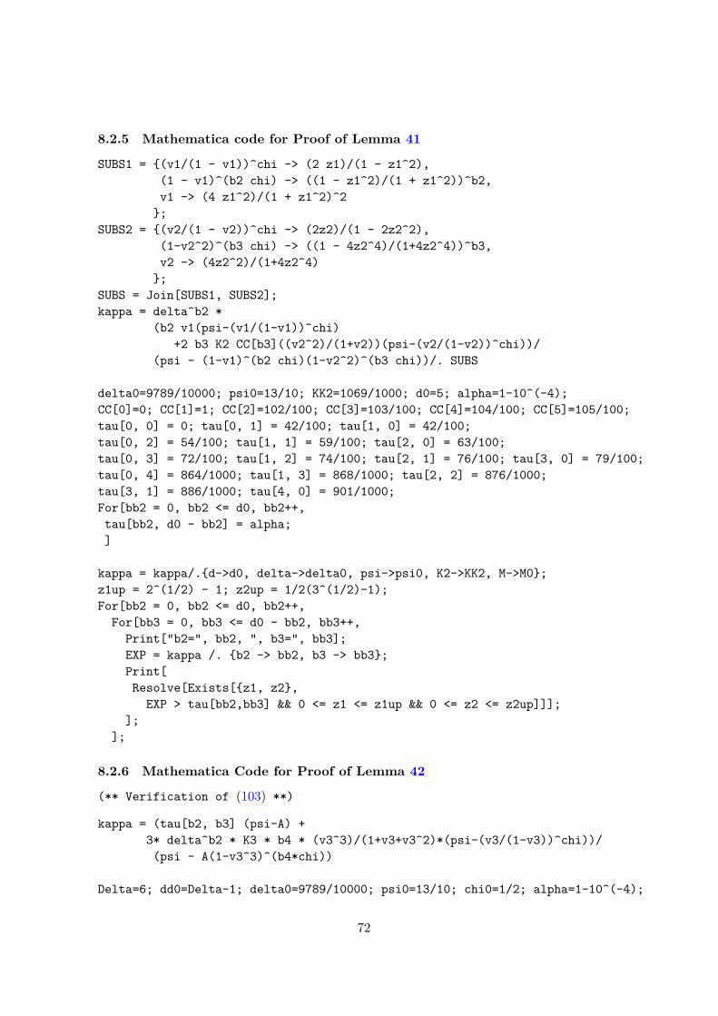
8.2.5 Mathematica code for Proof of Lemma 41

SUBS1 = (v1/(1 - v1))^chi -> (2 z1)/(1 - z1^2),(1 - v1)^(b2 chi) -> ((1 - z1^2)/(1 + z1^2))^b2,v1 -> (4 z1^2)/(1 + z1^2)^2;

SUBS2 = (v2/(1 - v2))^chi -> (2z2)/(1 - 2z2^2),(1-v2^2)^(b3 chi) -> ((1 - 4z2^4)/(1+4z2^4))^b3,v2 -> (4z2^2)/(1+4z2^4);

SUBS = Join[SUBS1, SUBS2];kappa = delta^b2 *

(b2 v1(psi-(v1/(1-v1))^chi)+2 b3 K2 CC[b3]((v2^2)/(1+v2))(psi-(v2/(1-v2))^chi))/

(psi - (1-v1)^(b2 chi)(1-v2^2)^(b3 chi))/. SUBS

delta0=9789/10000; psi0=13/10; KK2=1069/1000; d0=5; alpha=1-10^(-4);CC[0]=0; CC[1]=1; CC[2]=102/100; CC[3]=103/100; CC[4]=104/100; CC[5]=105/100;tau[0, 0] = 0; tau[0, 1] = 42/100; tau[1, 0] = 42/100;tau[0, 2] = 54/100; tau[1, 1] = 59/100; tau[2, 0] = 63/100;tau[0, 3] = 72/100; tau[1, 2] = 74/100; tau[2, 1] = 76/100; tau[3, 0] = 79/100;tau[0, 4] = 864/1000; tau[1, 3] = 868/1000; tau[2, 2] = 876/1000;tau[3, 1] = 886/1000; tau[4, 0] = 901/1000;For[bb2 = 0, bb2 <= d0, bb2++,tau[bb2, d0 - bb2] = alpha;]

kappa = kappa/.d->d0, delta->delta0, psi->psi0, K2->KK2, M->M0;z1up = 2^(1/2) - 1; z2up = 1/2(3^(1/2)-1);For[bb2 = 0, bb2 <= d0, bb2++,

For[bb3 = 0, bb3 <= d0 - bb2, bb3++,Print["b2=", bb2, ", b3=", bb3];EXP = kappa /. b2 -> bb2, b3 -> bb3;Print[Resolve[Exists[z1, z2,

EXP > tau[bb2,bb3] && 0 <= z1 <= z1up && 0 <= z2 <= z2up]]];];

];

8.2.6 Mathematica Code for Proof of Lemma 42

(** Verification of (103) **)

kappa = (tau[b2, b3] (psi-A) +3* delta^b2 * K3 * b4 * (v3^3)/(1+v3+v3^2)*(psi-(v3/(1-v3))^chi))/(psi - A(1-v3^3)^(b4*chi))

Delta=6; dd0=Delta-1; delta0=9789/10000; psi0=13/10; chi0=1/2; alpha=1-10^(-4);

72

tau[0, 0]=0; tau[0, 1]=42/100; tau[1, 0]=42/100;tau[0, 2]=54/100; tau[1, 1]=59/100; tau[2, 0]=63/100;tau[0, 3]=72/100; tau[1, 2]=74/100; tau[2, 1]=76/100; tau[3, 0]=79/100;tau[0, 4]=864/1000; tau[1, 3]=868/1000; tau[2, 2]=876/1000;tau[3, 1]=886/1000; tau[4, 0]=901/1000;tau[5, 0]=alpha;

kappa = kappa/.delta->delta0, psi->psi0, chi->chi0, K3->1160/1000For[bb2 = 0, bb2 <= dd0, bb2++,

For[bb3 = 1, bb3 <= dd0 - bb2, bb3++,For[bb4 = 1, bb4 <= dd0 - bb2 - bb3, bb4++,

Print["Running for b2=", bb2, " b3=", bb3, " and b4=", bb4];EXP = kappa /. b2 -> bb2, b3 -> bb3, b4 -> bb4;B = bb2 + bb3 + bb4;Print[Resolve[Exists[A, v3,EXP > tau[B, 0] && 0 <= v3 <= 1/2 && 0 <= A <= 1]]];

];];

];

(** Verification of (105) **)

SUBS = (v1/(1 - v1))^chi->u1, v1->(u1^2)/(1+u1^2), (v3/(1-v3))^chi->u3,v3->(u3^2)/(1+u3^2);

kappa = delta^b2 *( b2 v1 (psi - (v1/(1 - v1))^chi)+3*K3*b4*(v3^3)/(1+v3+v3^2)*(psi - (v3/(1 - v3))^chi))/(psi - (1-v1)^(b2*chi) (1-v3^3)^(b4*chi)) /. SUBS

Delta=6; dd0=Delta-1; delta0=9789/10000; psi0=13/10; chi0=1/2; alpha= 1-10^(-4);tau[1,0]=42/100; tau[2,0]=63/100; tau[3,0]=79/100; tau[4,0]=901/1000; tau[5,0]=alpha;

kappa = kappa /.delta->delta0, psi->psi0, chi->chi0, K3->1160/1000For[bb2 = 0, bb2 <= dd0, bb2++,

For[bb4 = 1, bb4 <= dd0 - bb2, bb4++,Print["Running for b2=", bb2, " and b4=", bb4];EXP = kappa/.b2 -> bb2, b3 -> bb3, b4 -> bb4;B = bb2 + bb4;Print[Resolve[Exists[u1, u3,

EXP > tau[B, 0] && 0 <= u1 <= 1 && 0 <= u3 <= 1]]];];

];

8.2.7 Mathematica Code for Proof of Lemma 43

The following code can be executed by copying it in a Mathematica cell.

73

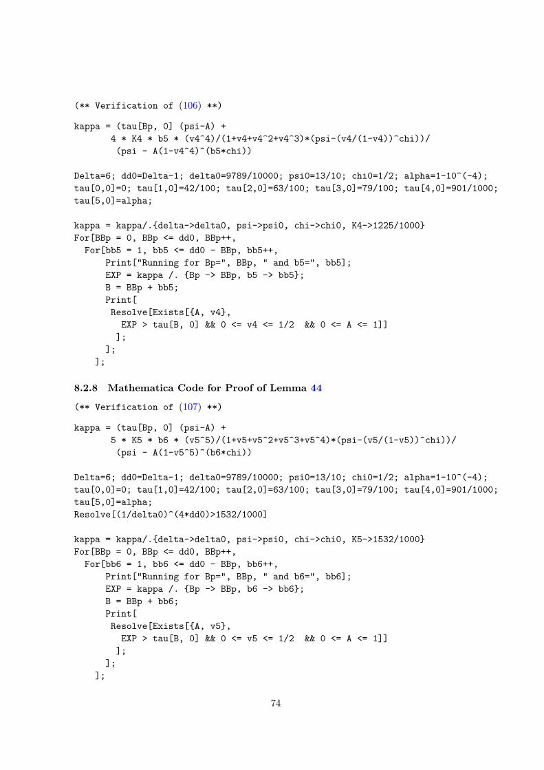
(** Verification of (106) **)

kappa = (tau[Bp, 0] (psi-A) +4 * K4 * b5 * (v4^4)/(1+v4+v4^2+v4^3)*(psi-(v4/(1-v4))^chi))/(psi - A(1-v4^4)^(b5*chi))

Delta=6; dd0=Delta-1; delta0=9789/10000; psi0=13/10; chi0=1/2; alpha=1-10^(-4);tau[0,0]=0; tau[1,0]=42/100; tau[2,0]=63/100; tau[3,0]=79/100; tau[4,0]=901/1000;tau[5,0]=alpha;

kappa = kappa/.delta->delta0, psi->psi0, chi->chi0, K4->1225/1000For[BBp = 0, BBp <= dd0, BBp++,

For[bb5 = 1, bb5 <= dd0 - BBp, bb5++,Print["Running for Bp=", BBp, " and b5=", bb5];EXP = kappa /. Bp -> BBp, b5 -> bb5;B = BBp + bb5;Print[Resolve[Exists[A, v4,EXP > tau[B, 0] && 0 <= v4 <= 1/2 && 0 <= A <= 1]]];

];];

8.2.8 Mathematica Code for Proof of Lemma 44

(** Verification of (107) **)

kappa = (tau[Bp, 0] (psi-A) +5 * K5 * b6 * (v5^5)/(1+v5+v5^2+v5^3+v5^4)*(psi-(v5/(1-v5))^chi))/(psi - A(1-v5^5)^(b6*chi))

Delta=6; dd0=Delta-1; delta0=9789/10000; psi0=13/10; chi0=1/2; alpha=1-10^(-4);tau[0,0]=0; tau[1,0]=42/100; tau[2,0]=63/100; tau[3,0]=79/100; tau[4,0]=901/1000;tau[5,0]=alpha;Resolve[(1/delta0)^(4*dd0)>1532/1000]

kappa = kappa/.delta->delta0, psi->psi0, chi->chi0, K5->1532/1000For[BBp = 0, BBp <= dd0, BBp++,

For[bb6 = 1, bb6 <= dd0 - BBp, bb6++,Print["Running for Bp=", BBp, " and b6=", bb6];EXP = kappa /. Bp -> BBp, b6 -> bb6;B = BBp + bb6;Print[Resolve[Exists[A, v5,EXP > tau[B, 0] && 0 <= v5 <= 1/2 && 0 <= A <= 1]]];

];];

74

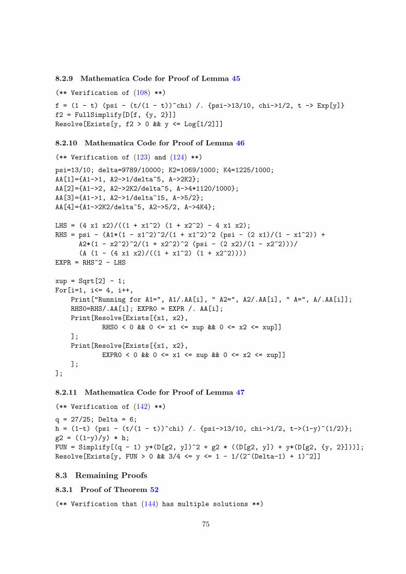
8.2.9 Mathematica Code for Proof of Lemma 45

(** Verification of (108) **)

f = (1 - t) (psi - (t/(1 - t))^chi) /. psi->13/10, chi->1/2, t -> Exp[y]f2 = FullSimplify[D[f, y, 2]]Resolve[Exists[y, f2 > 0 && y <= Log[1/2]]]

8.2.10 Mathematica Code for Proof of Lemma 46

(** Verification of (123) and (124) **)

psi=13/10; delta=9789/10000; K2=1069/1000; K4=1225/1000;AA[1]=A1->1, A2->1/delta^5, A->2K2;AA[2]=A1->2, A2->2K2/delta^5, A->4*1120/1000;AA[3]=A1->1, A2->1/delta^15, A->5/2;AA[4]=A1->2K2/delta^5, A2->5/2, A->4K4;

LHS = (4 x1 x2)/((1 + x1^2) (1 + x2^2) - 4 x1 x2);RHS = psi - (A1*(1 - x1^2)^2/(1 + x1^2)^2 (psi - (2 x1)/(1 - x1^2)) +

A2*(1 - x2^2)^2/(1 + x2^2)^2 (psi - (2 x2)/(1 - x2^2)))/(A (1 - (4 x1 x2)/((1 + x1^2) (1 + x2^2))))

EXPR = RHS^2 - LHS

xup = Sqrt[2] - 1;For[i=1, i<= 4, i++,

Print["Running for A1=", A1/.AA[i], " A2=", A2/.AA[i], " A=", A/.AA[i]];RHS0=RHS/.AA[i]; EXPR0 = EXPR /. AA[i];Print[Resolve[Exists[x1, x2,

RHS0 < 0 && 0 <= x1 <= xup && 0 <= x2 <= xup]]];Print[Resolve[Exists[x1, x2,

EXPR0 < 0 && 0 <= x1 <= xup && 0 <= x2 <= xup]]];

];

8.2.11 Mathematica Code for Proof of Lemma 47

(** Verification of (142) **)

q = 27/25; Delta = 6;h = (1-t) (psi - (t/(1 - t))^chi) /. psi->13/10, chi->1/2, t->(1-y)^(1/2);g2 = ((1-y)/y) * h;FUN = Simplify[(q - 1) y*(D[g2, y])^2 + g2 * ((D[g2, y]) + y*(D[g2, y, 2]))];Resolve[Exists[y, FUN > 0 && 3/4 <= y <= 1 - 1/(2^(Delta-1) + 1)^2]]

8.3 Remaining Proofs8.3.1 Proof of Theorem 52

(** Verification that (144) has multiple solutions **)

75

Delta = 17;lambda = 1/2; beta = 1/2; gamma = 1;Resolve[Exists[x, y,

x == lambda ((beta y + 1)/(y + gamma))^(Delta - 1) &&y == lambda ((beta x + 1)/(x + gamma))^(Delta - 1) && x > 0 &&y > 0 && x > y]]

76