Senior Thesis

An Investigation of the Hydrogeologic Connections Among the Scioto River, the GlaciaJ-Outwash Aquifer, and the Carbonate Aquifer at the South Well Field,

Southern Franklin County, Ohio.

by

Stephen Joseph Champa

Submitted as partial fulf1llment of the requirements for the degree of Bachelor of Science in Geology and M1neralogy at The Oh1o State University.

Winter Quarter 1989.

Appr~vitW Dr. E. Scott Bair

Acknowledgements

I would like to thank Dr. E. Scott Bair of The Ohio State University for the suggestion of this project and his assistance and advice. I would also like to thank my parents for their support throughout my college career. Special appreciation goes to my wife Carol for her love, support,and patience.

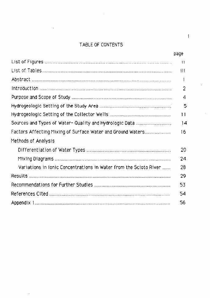
TABLE OF CONTENTS

page

List of Figures ...................................................................................................................... 11

List of Tables............................................................................................................................. iii

Abstract ..................................................................................................................................... .

Introduction ............................................................................................................................... 2

Purpose and Scope of Study ................................................................................................ 4

Hydrogeologic Setting of the Study Area .................................................................... : 5

Hydrogeologic Setting of the Collector Wells........................................................... 11

Sources and Types of Water- Oual ity and Hydro logic Data.................................. 14

Factors Affecting Mixing of Surface Water and Ground Waters......................... 16

Methods of Analysis

Differentiation of Water Types................................................................................. 20

Mixing Diagrams ............................................................................................................... 24

Variations in Ionic Concentrations in Water from the Scioto River........ 28

Results ........................................................................................................................................ 29

Recommendations for Further Studies......................................................................... 53

References Cited .................................................................................................................... 54

Appendix 1.................................................................................................................................. 56

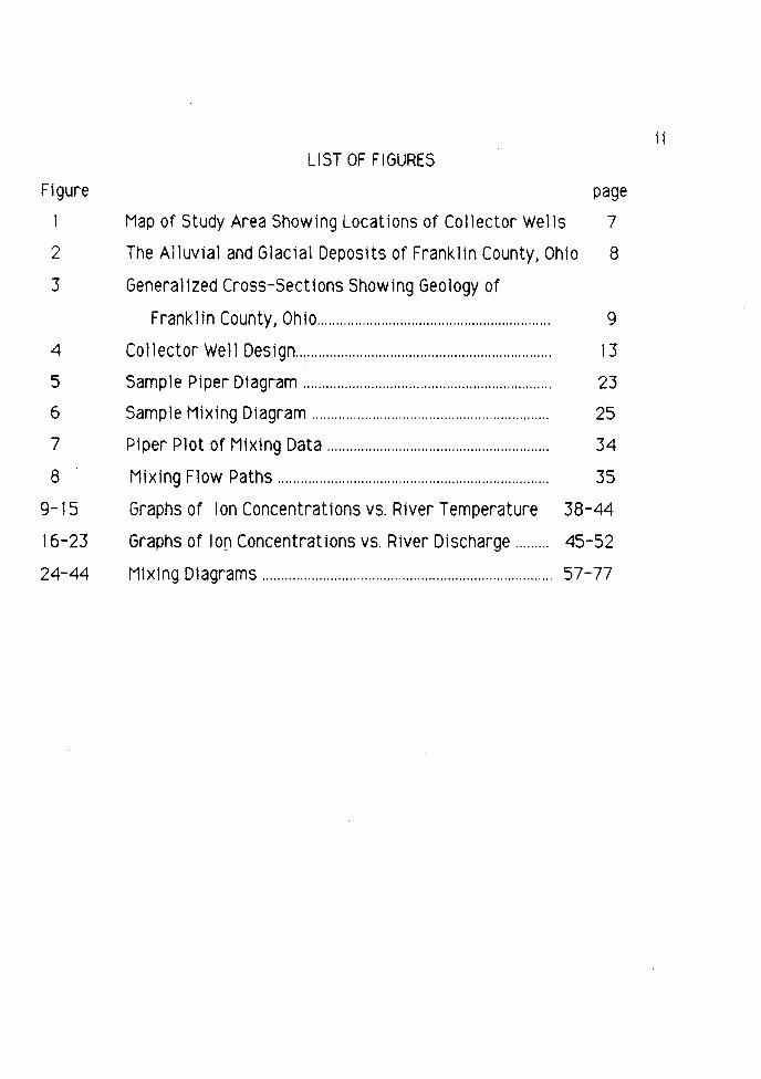
LI ST OF FIGURES

Figure page

1 Map of Study Area Showing Locations of Collector Wells 7

2 The Alluvial and Glacial Deposits of Franklin County, Ohio 8

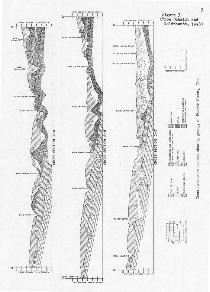
3 Generalized Cross-Sections Showing Geology of

Franklin County, Ohio.............................................................. 9

4 Collector Weil Design.................................................................... 13

5

6

7

8

9-15

16-23

24-44

Sample Piper Diagram ................................................................. .

Sample Mixing Diagram ............................................................. ..

Piper Plot of Mixing Data ......................................................... ..

Mixing Flow Paths ...................................................................... ..

Graphs of Ion Concentrations vs. River Temperature

23

25

34

35

38-44

Graphs of lo[) Concentrations vs. River Discharge......... 45-52

M1x1ng Diagrams ............................................................................. 57-77

ii

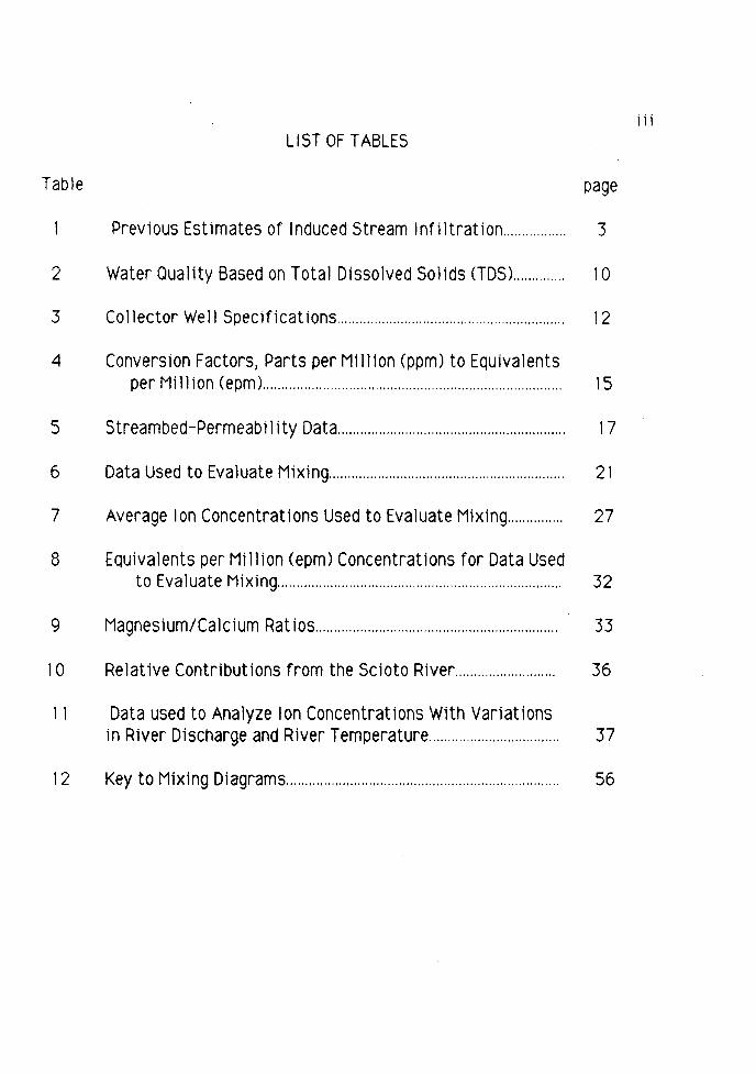
iii LI ST OF TABLES

Table page

Previous Estimates of Induced Stream Infiltration................. 3

2 Water Qual1ty Based on Total Dissolved Solids <TDSL........... 1 o

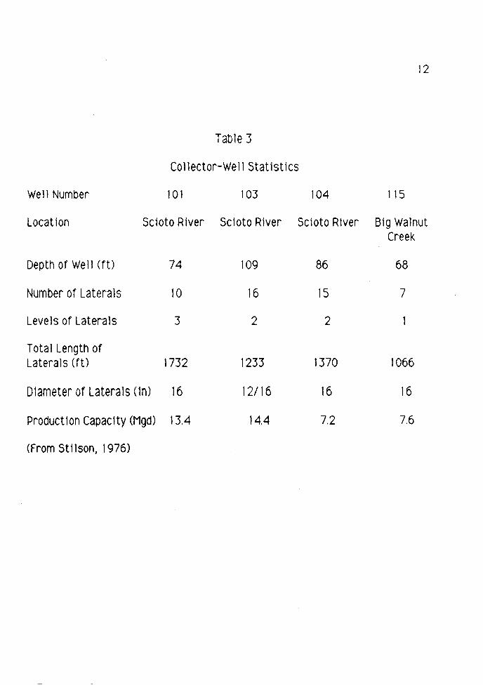
3 Collector Well Specifications............................................................. 12

4 Conversion Factors, Parts per Million (ppm) to Equivalents per Million (epm)................................................................................ 15

5 Streambed-Permeability Data............................................................. 17

6 Data Used to Evaluate Mixing............................................................... 21

7 Average Ion Concentrations Used to Evaluate Mixing............... 27

8 Equivalents per Million (epm) Concentrat1ons for Data Used to Evaluate Mixing............................................................................ 32

9 Magnesium/Calcium Ratios................................................................. 33

1 O Relative Contributions from the Scioto River........................... 36

11 Data used to Analyze Ion Concentrations With Variations in River Discharge and River Temperature................................... 37

12 Key to Mixing Diagrams......................................................................... 56

ABSTRACT

Th1s study was conducted to determ1ne the relat1ve contr1but1ons from the

glac1al-outwash aquifer, upward leakage from the carbonate aquifer, and induced

stream infiltration from the Scioto River to the three radial-collector wells

located along the east floodplain of the Scioto River 1n Southern Franklin County,

Ohio. These wells are used for municipal purposes by the county and by the City of

Columbus and provide about 15 percent of the local water supply.

The study is based on water-quality analyses of samples of the various source

waters. Potential mixing of the source waters in the collector wells was

analyzed using the results of ten samples from the Scioto River, three samples

from the collector wells, five samples from the glacial-outwash aquifer, and

seven samples from the carbonate aquifer. Piper diagrams, ratio studies and

mixing diagrams were used to determine if mixing Is occurring. For ions which

indicated mixing calculations of the relative contributions were performed using

the mixing equation.

Results Indicate that induced stream tnfi ltration from the Scioto River

accounts for about 26 percent of the water produced by the collector wells. No

contribution from the carbonate aquifer was Indicated by the mixing evaluations.

Variations in ion concentrations in the Scioto River with changes in water

temperature and river discharge also were examined. Graphs were constructed of

Ion concentration versus rtver discharge and versus river water temperature.

These studies show that ion concentrations tend to increase as temperature

decreases, and to increase as river discharge increases. These trends in water

quality in the river should be reflected in the water produced by the collector

wells due to induced stream infiltration.

2

INTRODUCTION

In 1978 the City of Columbus, Ohio, began construction of four radial-collector

wells in southern Franklin County. Three of these wells are located along the

floodpla1n of the Sc1oto R1ver and one well 1s located along the floodpla1n of B1g

Walnut Creek. These wells are completed 1n a permeable, glacial-outwash, sand

and gravel. The collector wells are used for municipal purposes and supply about

15 percent of the C1ty's water. The wells normally produce about 8.2 million

gallons per day <Mgd), but are capable of producing about 25 Mgd.

The wells were designed to make use of induced inf11tration from the Scioto

River and Big Walnut Creek. Initial studies performed by Stilson and Associates

< 1976) predicted that 80 percent of the water produced by the wells would be

induced lnf1ltrat1on from the two streams. This would mean that relatively little

water would be removed from storage in the glacial-outwash aquifer. If, however,

the lower estimates of induced stream infiltration calculated by more recent

studies <Table 1) are correct, then a significantly greater amount of water must

be removed from aquifer storage, especially during times of peak demand. This

would cause the cone of depression created by the pumping of the wells to expand,

thereby increasing the capture zone of the wells. If the capture zone of the wells

were extended far enough it m1ght then incorporate State Routes 23 and 104 which

run north and south to the east and west of the study area <Fig. 1 ). These are

potential sources of contam1nant sp11ls, and burled gas tanks at serv1ce stat1ons

along Route 23 m1ght also leak into the flow system.

Potential sources of water to the wells are induced infiltration from the

Scioto River and Big Walnut Creek, water from storage in the glacial-outwash

aquifer, and upward leakage from the carbonate bedrock aquifer into the overlying

glacial-outwash aqu1fer.

3

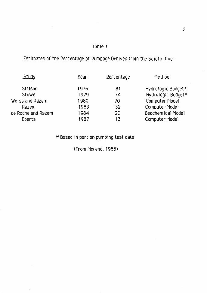
Table 1

Est 1mates of the Percentage of Pumpage Derived from the Scioto River

Study Yfa[ percentage Method

Stilson 1976 81 Hydro logic Budget* Stowe 1979 74 Hydro logic Budget*

Weiss and Razem 1980 70 Computer Model Raz em 1983 32 Computer Model

de Roche and Razem 1984 20 Geo chemical Model Eberts 1987 13 Computer Model

*Based in part on pumping test data

<From Moreno, 1988)

4

PURPOSE AND SCOPE OF STUDY

In light of the residential, commercial, and industrial growth in the Columbus

area, it is becoming increasingly necessary for city and county officials to be

aware of ava11ab le water resources. This report presents the results of a study to

determine the relative contributions from the various potential sources of water

to the collector wells. These sources include the g1acial-outwash aquifer,

potential upward leakage from the carbonate bedrock aquifer, and induced

inf11tration from the Scioto River and Big Walnut Creek.

The mixing of these waters is analyzed on the basis of major-ion chemistry.

Fluctuations in the concentrations of dissolved calcium, magnesium, sodium,

potassium, chloride, sulfate, and bicarbonate due to changes in river temperature

and river discharge also are examined. Due to the limitations of the available

data, only the three collector wells along the Scioto River are considered.

5

HYDROGEOLOG IC SETT I NG OF THE STUDY AREA

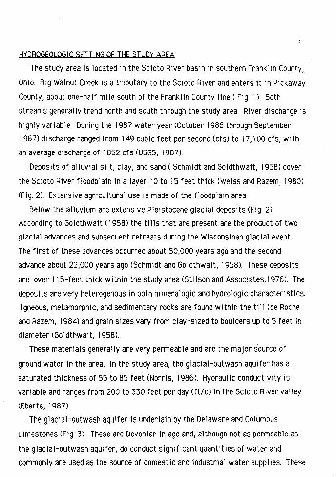
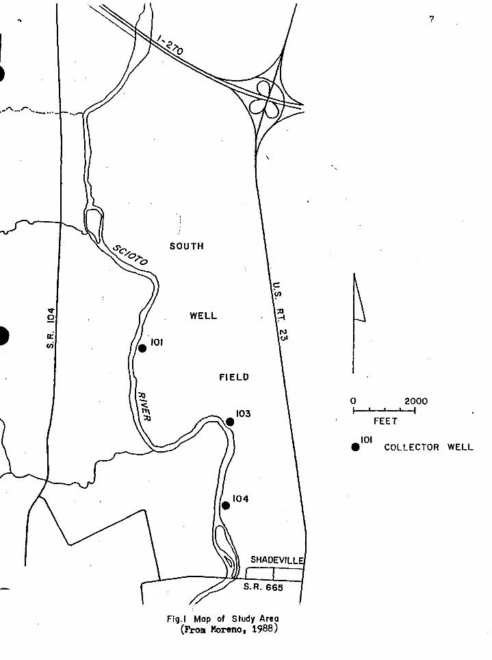
The study area is located in the Scioto River basin in southern Franklin County,

Ohio. Big Walnut Creek is a tributary to the Scioto River and enters 1t in Pickaway

County, about one-half mile south of the Franklin County line (Fig. 1 ). Both

streams generally trend north and south through the study area. River discharge is

highly variable. During the 1987 water year (October 1986 through September

1987) discharge ranged from 149 cubic feet per second (cfs) to 17, 100 cfs, with

an average discharge of 1852 cfs <USGS, 1987).

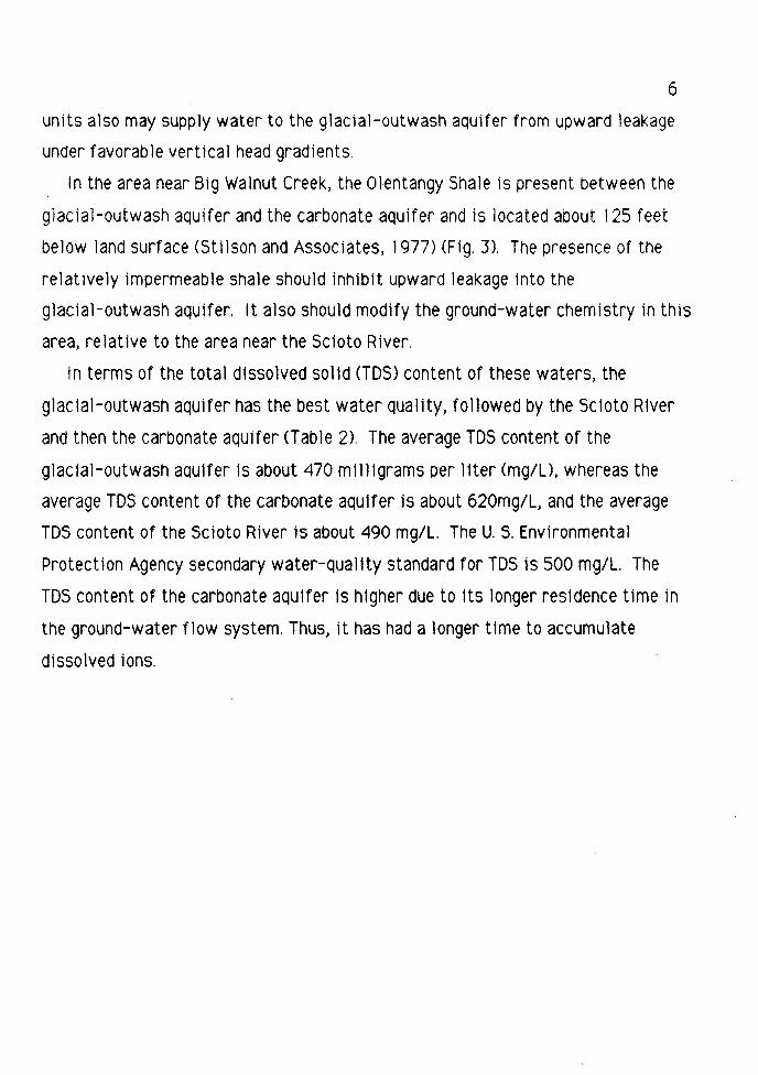
Deposits of alluvial si It, clay, and sand< Schmidt and Goldthwait, 1958) cover

the Scioto River floodplain in a layer 1 o to 15 feet thick (Weiss and Razem, 1980)

(Fig. 2). Extensive agricultural use is made of the floodplain area.

Below the alluv1um are extensive Pleistocene glacial depos1ts <Fig. 2).

According to Goldthwait< 1958) the tills that are present are the product of two

glacial advances and subsequent retreats during the Wisconsinan glacial event.

The first of these advances occurred about 50,000 years ago and the second

advance about 22,000 years ago (Schmidt and Goldthwait, 1958). These deposits

are over 115-feet thick within the study area <Stilson and Associates, 1976). The

deposits are very heterogenous 1n both m1neralogic and hydrologic characteristics.

Igneous, metamorphic, and sedimentary rocks are found within the till (de Roche

and Razem, 1984) and grain sizes vary from clay-sized to boulders up to 5 feet In

diameter (Goldthwait, 1958).

These materials generally are very permeable and are the major source of

ground water in the area. In the study area, the glacial-outwash aquifer has a

saturated thickness of 55 to 85 feet (Norris, 1986). Hydraulic conductivity is

variable and ranges from 200 to 330 feet per day (ft/d) in the Scioto River valley

(Eberts, 1987).

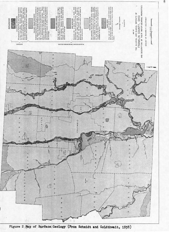
The glac1al-outwash aquifer is underlain by the Delaware and Columbus

L 1mestones (Ftg. 3). These are Devon tan ln age and, although not as permeable as

the glacial-outwash aquifer, do conduct significant quantities of water and

commonly are used as the source of domestic and industrial water supplies. These

6

units also may supply water to the glacial-outwash aquifer from upward leakage

under favorable vertical head gradients.

In the area near Big Walnut Creek, the Olentangy Shale is present between the

giacial-outwash aquifer and the carbonate aquifer and is located about 125 feet

below land surface (Stilson and Associates, 1977) CF lg. 3). The presence of the

relatively impermeable shale should inhibit upward leakage into the

glacial-outwash aquifer. It also should modify the ground-water chemistry in this

area, relative to the area near the Scioto River.

In terms of the total dissolved solid <TDS) content of these waters, the

glacial-outwash aquifer has the best water quality, followed by the Scioto River

and then the carbonate aquifer <Table 2). The average TDS content of the

glacial-outwash aquifer is about 470 m11ligrams per liter Cmg/U, whereas the

average TDS content of the carbonate aquifer is about 620mg/L, and the average

TDS content of the Scioto River is about 490 mg/L. The U. S. Environmental

Protection Agency secondary water-quality standard for TDS is 500 mg/L. The

TDS content of the carbonate aquifer is higher due to its longer residence time in

the ground-water flow system. Thus, 1t has had a longer time to accumulate

dissolved ions.

..

-""·-,,-···-···

'·

SOUTH

WELL

FIELD

SHAOEVILL

Fig.I Map of Study Area (From Moreno, 1988)

7

0 2000 I I

FEET

IOI • COLLECTOR WELL

AN

D

\, D

ra.1

na1

• C

ba

.nn

eb

Gra

vel

Pit

MAP~

OF

GLA

CIA

L D

EP

OS

ITS

TH

E ALL

UVIA~l

~NDCOU

NTY.

OH

IOP

RO

PE

RT

IES

F

RA

NK

T

HE

IR

WA

TE

R-B

EA

RIN

G

DE

SC

RIP

TIO

N

OF

GO

LD

TH

WA

IT

GEO

LOG

Y

BY

RIC

HA

RD

P.

i

-

11~]1 •lS ]1'08'f' 1.1.)]J NI 1 Jon1111 •

<..:> __ §r-..,...~--r~""""l"':"""~~;;.\'1§ ~~-.,~

,3iiJl yjS JllOU 'HJ~ NI ']001111\'

9 Figure 3

(From Schmidt and Goldthwa~t~ 1958)

0 :.c 0

-0

>­O'I 0 0 Q)

O'I

O'I c 'i 0

..c (/)

(/)

c .Q u Q) (/)

(/) (/)

0 i.... u -0 Q)

.~

2 Q) c Q)

(.!)

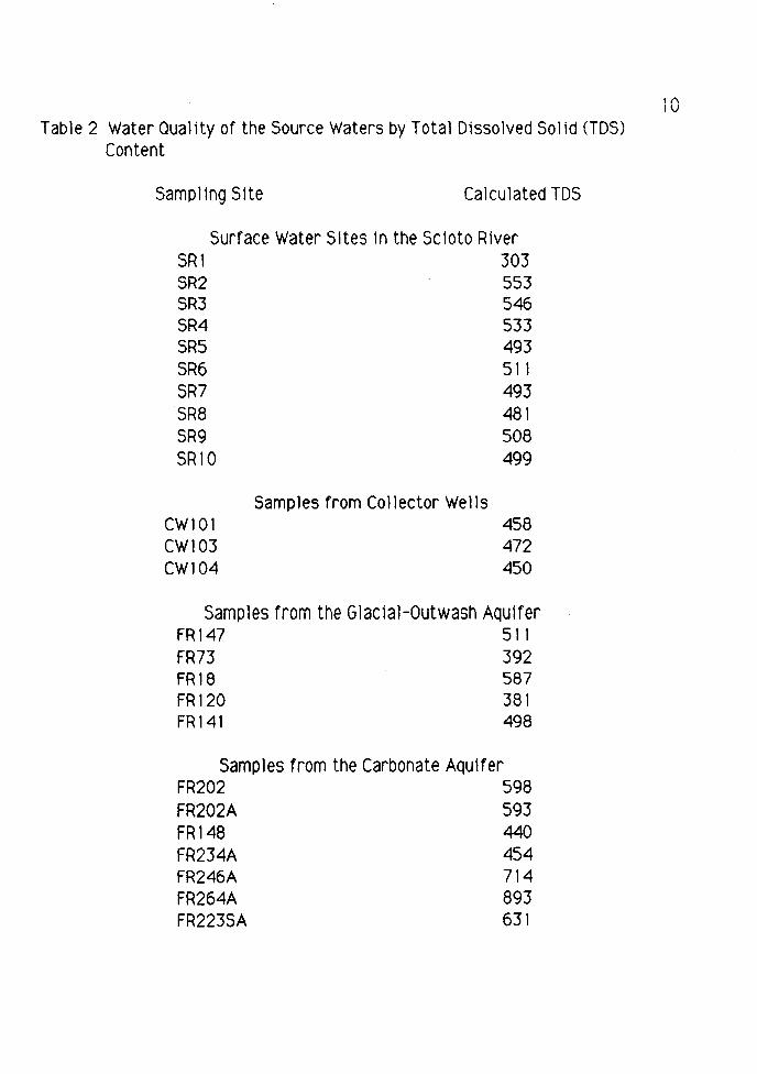
Table 2 Water aual1ty of the Source Waters by Total Dissolved Solid <TDS) Content

Sampling Site Calculated TDS

Surface Water Sites 1n the Sc1oto River SRl SR2 SR3 SR4 SR5 SR6 SR7 SR8 SR9 SR10

CW101 CW103 CW104

Samples from Collector Wells

303 553 546 533 493 511 493 481 508 499

458 472 450

Samples from the Glac1al-Outwash Aquifer FR147 511 FR73 392 FR18 587 FR120 381 FR141 498

Samples from the Carbonate Aquifer FR202 598 FR202A 593 FR148 440 FR234A 454 FR246A 714 FR264A 893 FR223SA 631

1 ('\ IV

11

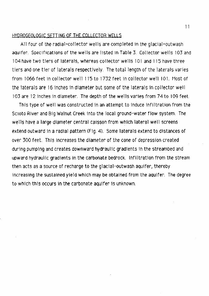
HYDROGEOLOG IC SETT I NG OF THE COLLECTOR WELLS

All four of the radial-collector wells are completed in the glacial-outwash

aquifer. Specifications of the wells are listed in Table 3. Collector wells 103 and

104 have two t1ers of laterals, whereas collector wells 1o1 and 115 have three

tiers and one tier of laterals respectively. The total length of the laterals varies

from 1066 feet in collector well 115 to 1732 feet in collector well 1O1. Most of

the laterals are 16 inches 1n diameter but some of the laterals in collector well

103 are 12 inches in diameter. The depth of the wells varies from 74 to 109 feet.

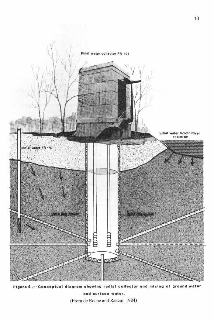
This type of well was constructed in an attempt to induce infiltration from the

Scioto River and Big Walnut Creek into the local ground-water flow system. The

wells have a large diameter central caisson from which lateral well screens

extend outward in a radial pattern <Fig. 4). Some laterals extend to distances of

over 300 feet. This increases the diameter of the cone of depression created

during pumping and creates downward hydraulic gradients 1n the streambed and

upward hydraulic gradients in the carbonate bedrock. Infiltration from the stream

then acts as a source of recharge to the glacial-outwash aquifer, thereby

increasing the sustained yield which may be obtained from the aquifer. The degree

to which this occurs 1n the carbonate aquifer ts unknown.

12

T"'b le 7 I a I .J

Collector-Well Statistics

Well Number 101 103 104 115

Location Scioto River Scioto River Scioto River Big Walnut Creek

Depth of Well (ft) 74 109 86 68

Number of Laterals 10 16 15 7

Levels of Laterals 3 2 2

Total Length of Laterals (ft) 1732 1233 1370 1066

D1ameter of Laterals (1n) 16 12/16 16 16

Production Capacity (Mgd) 13.4 14.4 7.2 7.6

(from Stilson, 1976)

.· · ... : . ~ :·.·:'. :; ', ; .• . ·.' .

·)~·) ·:~-: >· ~ :" ·:·

Final water collector FR-101

11. "

13

Figure 4 .--Conceptual diagram showing radlal collector and mixing of ground water

and surface water.

(From de Roche and Razem, 1984)

14

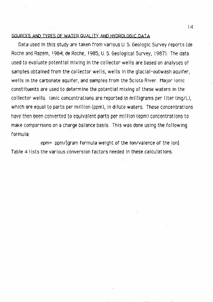
SOURCES AND TYPES OF WATER QUALITY AND HYDROLOG!C DATA

Data used in this study are taken from various U. 5. Geologic Survey reports (de

Roche and Razem, 1984; de Roche, 1985; U.S. Geological Survey, 1987). The data

used to evaluate potential mixing in the collector wells are based on analyses of

samples obtained from the collector wells, wells in the glacial-outwash aquifer,

wells in the carbonate aquifer, and samples from the Scioto River. Major ionic

constituents are used to determine the potential mixing of these waters in the

collector wells. Ionic concentrations are reported in milligrams per 1 iter Cmg/U,

which are equal to parts per million (ppm), in dilute waters. These concentrations

have then been converted to equivalent parts per million (epm) concentrations to make comparisons on a charge balance basis. This was done using the following

formula:

epm= ppm/[gram formula we1ght or the Jon/valence of the Jon]

Table 4 lists the variou~s conversion factors needed in these calculations.

15

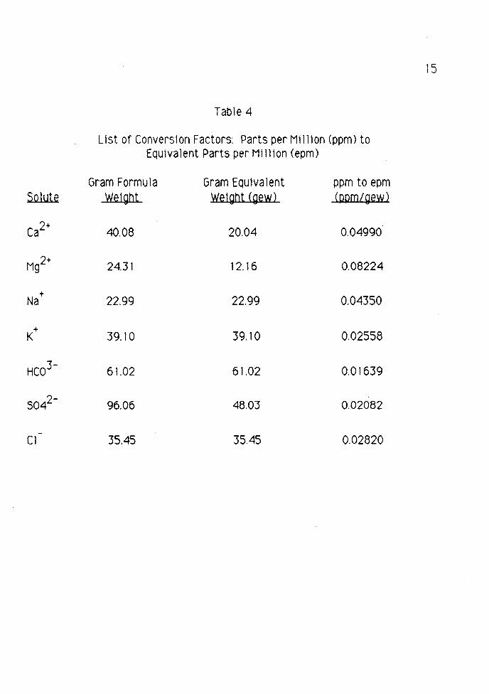
Table 4

List of Conversion Factors: Parts per Mill ion (ppm) to Equivalent Parts per Million (epm)

Gram Formula Gram Equ1valent ppm to epm Solute We1ght Weight Cgew) (ppm/gew)

ca2+ 40.08 20.04 0.04990

Mg2+ 24.31 12.16 0.08224

+ Na 22.99 22.99 0.04350

+ 39.10 0.02558 K 39.10

HC03- 61.02 61.02 0.01639

5042- 96.06 48.03 0.02082

Cl 35.45 35.45 0.02820

16

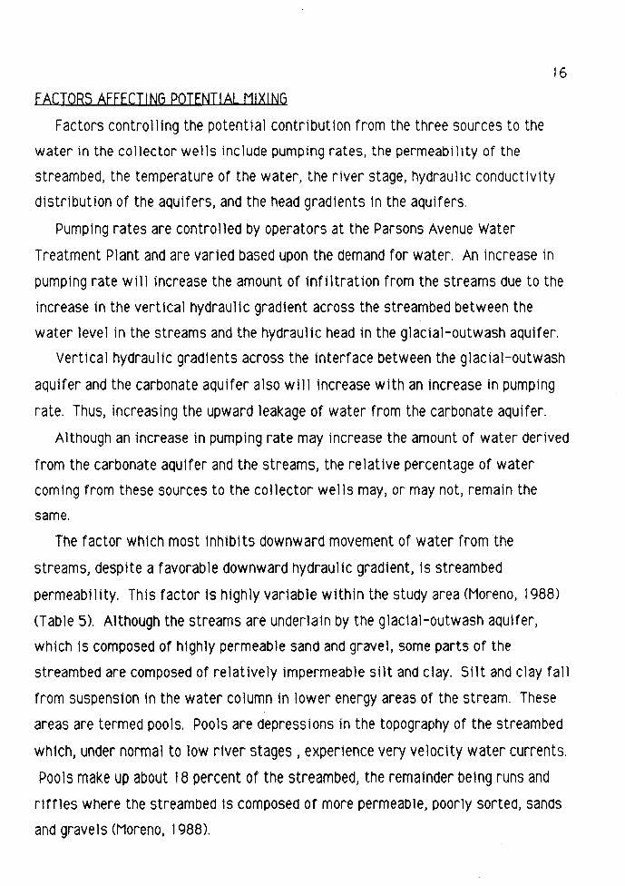
FACTORS AFFECTING POTENTIAL MIXING

Factors controlling the potential contribution from the three sources to the

water in the collector wells include pumping rates, the permeability of the

stream bed, the temperature of the water, the r1ver stage, hydraul 1c conduct 1v1ty

distribution of the aquifers, and the head gradients in the aquifers.

Pumping rates are controlled by operators at the Parsons Avenue Water

Treatment Plant and are varied based upon the demand for water. An increase in

pumping rate will increase the amount of infiltration from the streams due to the

increase in the vertical hydraul1c grad1ent across the streambed between the

water level in the streams and the hydraullc head in the glacial-outwash aquifer.

Vertical hydraulic gradients across the interface between the glacial-outwash

aquifer and the carbonate aquifer also will increase with an increase in pumping

rate. Thus, increasing the upward leakage of water from the carbonate aquifer.

Although an increase in pumping rate may increase the amount of water derived

from the carbonate aquifer and the streams, the relative percentage of water

coming from these sources to the collector wells may, or may not, remain the

same.

The factor which most inhibits downward movement of water from the

streams, despite a favorable downward hydraulic gradient, is streambed

permeability. This factor is highly variable within the study area (Moreno, 1988)

<Table 5). Although the streams are underla1n by the glac1al-outwash aquifer,

which is composed of highly permeable sand and gravel, some parts of the

streambed are composed of relatively impermeable silt and clay. Silt and clay fall

from suspension in the water column in lower energy areas of the stream. These

areas are termed pools. Pools are depressions in the topography of the streambed

which, under normal to low river stages, experience very velocity water currents.

Pools make up about 18 percent of the streambed, the remainder being runs and

rirnes where the streambed 1s composed or more permeable, poorly sorted, sands

and gravels <Moreno, 1988).

17

Downward infiltration also is affected by the temperature of the river water.

Viscosity is the resistance of a fluid to flow, and, in the case of water, is

inversely proportional to the temperature of the water. Consequently, water in

the Scioto Rtver and Big Walnut Creek should infiltrate downward more readily at

higher water temperatures during the summer months than at low water

temperatures during the winter months.

·River stage has two effects on the downward infiltration of stream water.

Both of these effects relate to the cross-sectional area, or geometry, of the

streambed. For the purposes of this discussion only a simple analysis is necessary.

An increase in stream width during higher river stages means that more of the

streambed ls covered by water. Because streambed permeab111ty 1s h1ghly

variable, this could cause significant changes in the amount of water moving

downward under favorable hydraulic gradients. Increased river stage also would

increase the driving head of the water at any point on the streambed. This would

increse the downward force on water particles and would enhance their downward

movement. Likewise, a drop in river stage would lessen the driving head and the

downward force would be less. The amount of water that can move downward into

the glac1al-outwash aquifer from the streams is controlled by the hydraulic

conducttv1ty of the streambed and the vert1cal hydrau11c gradient across the

streambed. The temperature of the surface water also affects the hydraulic

conductivity of the streambed.

The hydraulic conductivity of the carbonate aquifer is lower than it is in the

g1ac1al-outwash aqulfer. Thls means that as water in the glacial-outwash aquifer

moves toward the collector wells some of it is replaced by upward leakage from

the carbonate aquifer under favorable vertical hydraulic gradients. The rest of the

water must come from storage in the glacial-outwash aquifer.

Because the Scioto River ls the regional discharge area for the carbonate

aquifer, natural upward hydraulic gradients exist below the Scioto River within

the carbonate aquifer. These upward hydraulic gradients are enhanced by pumping

the collector wells. Thus, upward leakage from the carbonate aquifer will be

greatest below the collector wells, and particularly below the lateral well

screens which extend below the r1ver. The natural upward leakage ls, in part,

controlled by the ground-water level, or driving head, in the aquifer at its

recharge area located to the west of the study area.

18

19

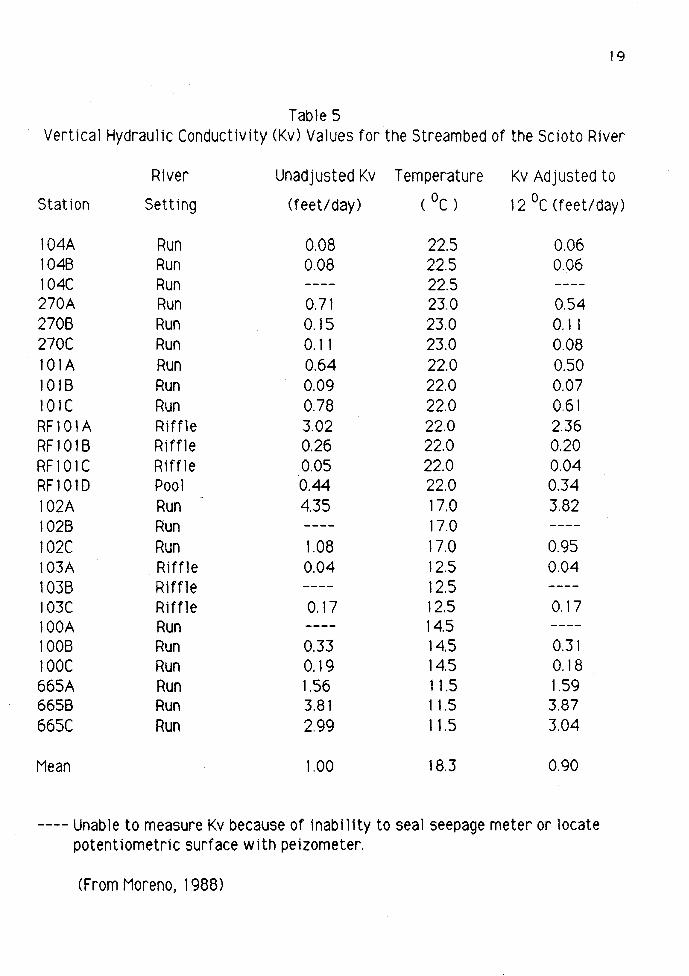
Table 5 Vertical Hydraulic Conductivity CKv) Values for the Streambed of the Scioto River

River Unadjusted Kv Temperature Kv Adjusted to

Station Setting (feet/day) ( oc ) 12 °c (feet/day)

104A Run 0.08 22.5 0.06 1048 Run 0.08 22.5 0.06 104C Run 22.5 270A Run 0.71 23.0 0.54 2708 Run 0.15 23.0 0.11 270C Run 0.11 23.0 0.08 101A Run 0.64 22.0 0.50 1018 Run 0.09 22.0 0.07 101C Run 0.78 22.0 0.61 RF101A Riffle 3.02 22.0 2.36 Rf 1018 Riffle 0.26 22.0 0.20 RF101C Riffle 0.05 22.0 0.04 RF101D Pool 0.44 22.0 0.34 102A Run 4.35 17.0 3.82 1028 Run 17.0 102C Run 1.08 17.0 0.95 103A Riffle 0.04 12.5 0.04 1038 R1ffle 12.5 103C Riffle 0.17 12.5 0.17 lOOA Run 14.5 1008 Run 0.33 14.5 0.31 lOOC Run 0.19 14.5 0.18 665A Run 1.56 11.5 1.59 6658 Run 3.81 11.5 3.87 665C Run 2.99 11.5 3.04

Mean 1.00 18.3 0.90

----Unable to measure Kv because of inabi 11ty to seal seepage meter or locate potentiometric surface with peizometer.

(From Moreno, 1988)

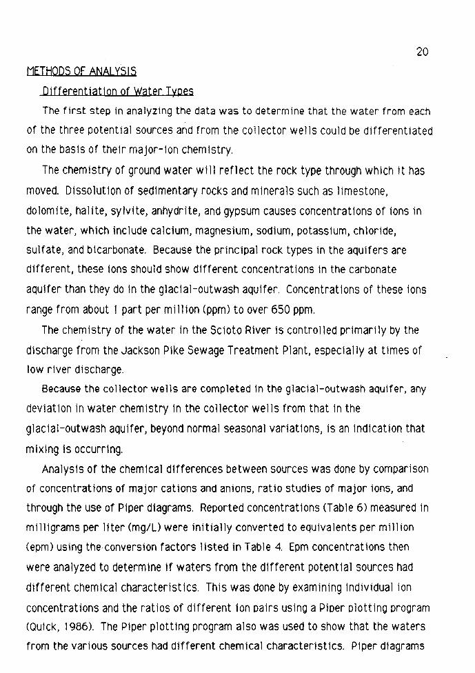
METHODS OF ANALYSIS

Differentiation of Water Types

20

The first step in analyzing the data was to determine that the water from each

of the three potential sources and from the collector wells could be differentiated

on the bas1s of the1r major-1on chem lstry.

The chemistry of ground water will reflect the rock type through which it has

moved. Dissolution of sedimentary rocks and minerals such as limestone,

dolomite, halite, sylvite, anhydrite, and gypsum causes concentrations of ions in

the water, which include calcium, magnesium, sodium, potassium, chloride,

sulfate, and bicarbonate. Because the principal rock types in the aquifers are

different, these ions should show different concentrations in the carbonate

aquifer than they do in the glacial-outwash aquifer. Concentrations of these ions

range from about 1 part per million (ppm) to over 650 ppm.

The chemistry of the water in the Scioto River is controlled primarily by the

discharge from the Jackson Pike Sewage Treatment Plant, especially at times of

low river discharge.

Because the collector wells are completed in the glacial-outwash aquifer, any

deviation in water chemistry in the collector wells from that in the

glac1al-outwash aquifer, beyond normal seasonal variations, is an indication that

mixing is occurring.

Analysis of the chemical differences between sources was done by comparison

of concentrations of major cations and anions, ratio studies of major ions, and

through the use of Piper diagrams. Reported concentrations <Table 6) measured in

milligrams per liter (mg/U were initially converted to equivalents per million

(epm) using the conversion factors listed in Table 4. Epm concentrations then

were analyzed to determine if waters from the different potential sources had

different chemical characteristics. This was done by examining individual ion

concentrations and the ratios of different ion pairs using a Piper plotting program

(Qu1ck, 1986). The Piper plotting program also was used to show that the waters

from the various sources had different chemical characteristics. Piper diagrams

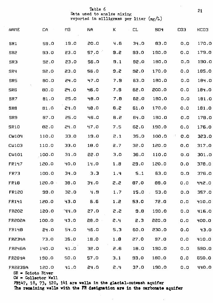
Table 6 21 n:tta used to analze mixing reported in milligrams per liter (mg/L)

NAME CA MG NA K CL SOLf C03 HC03

SRl 59.0 19.0 2a.a Lf .6 3Y:.a 83.a o.a 170.a

SR2 93.0 23.a 57.0 9.2 93.0 190.0 o.a 179.0

SR3 92.0 23.0 56.0 9 .1 92.0 180.0 0.0 190.0

SRY: 92.0 23.0 56.0 9.2 92.0 170.0 0.0 185.0

SRS 80.0 2Y:.O Lf7.0 7.9 63.0 180.a o.o 181.f.a

SR6 80.a 21.f.0 Lf6.a 7.9 62.0 200.a 0.0 181.f.O

SR7 81.0 25.a Lf8.a 7.8 62.a 180.0 o.o 181.0

SR8 81.0 21.f.a Y:8.a 8.2 61.a 170.a a.a 181.a

SR9 87.0 25.0 Lf6.a 8.2 61.f .0 19a.o a.a 178.a

SR la 82.a 2Y:.a Lf7.a 7.5 62.a 19a.a a.a 176.a

CWlOY: 11a.o 33.a 19.0 2.1 35.0 100.a a.a 323.0

CW1a3 11a.a 33.a 18.0 2.7 32.0 12a.o a.o 317.0

CWlOl 1oa.o 31.0 22.0 3.a 36.0 11a.o 0.0 301.a

FR1Lf7 120.0 LfO.O 11.f.0 1.8 29.0 120.0 0.0 378.0

FR73 1oa.o 31.f.a 3.3 1 . Lf 5.1 63.0 a.o 376.0

FR18 120.0 38.0 31.f .0 2.2 87.0 88.0 a.o LfLf2.a

FR120 99.a 32.a Lf .9 1.7 15.0 53.0 o.a 357.0

FRlLfl 120.0 Lf3.0 6.6 1.2 53.0 72.0 0.0 Lfla.O

FR202 120.a 'LfLf. a 27.a 2.2 9.8 190.a a.a Lf16.0

FR202A 100.0 Lf3.a 28.a 2.Lf 2.3 220.a a.a Lfaa.o

FR1Lf8 21.f.0 51.f.a Lf6.a 5.3 60.a 230.0 a.a Lf3.a

FR23LfA 73.0 35.0 18.a 1.8 27.a 97.a a.a Lfla.a

FR2Y:6A lY:O.O Lfl. 0 32.a 2.6 18.a 19a.a a.a 59a.a

FR26Y:A 190.0 so.a 57.a 3.1 93.0 180.a o.o 650.0

FR223SA 120.0 Y:l.O 2Lf .a 2.Y: 37.0 19a.a a.a Y:Y:a.a SR • Scioto River CW • Collector Well Ffi147, 18, 73, 120, 141 are wells in the glacial-outwash aquifer 'lhe remaining wells with the FR designation are in the oarbonate aquifer

22

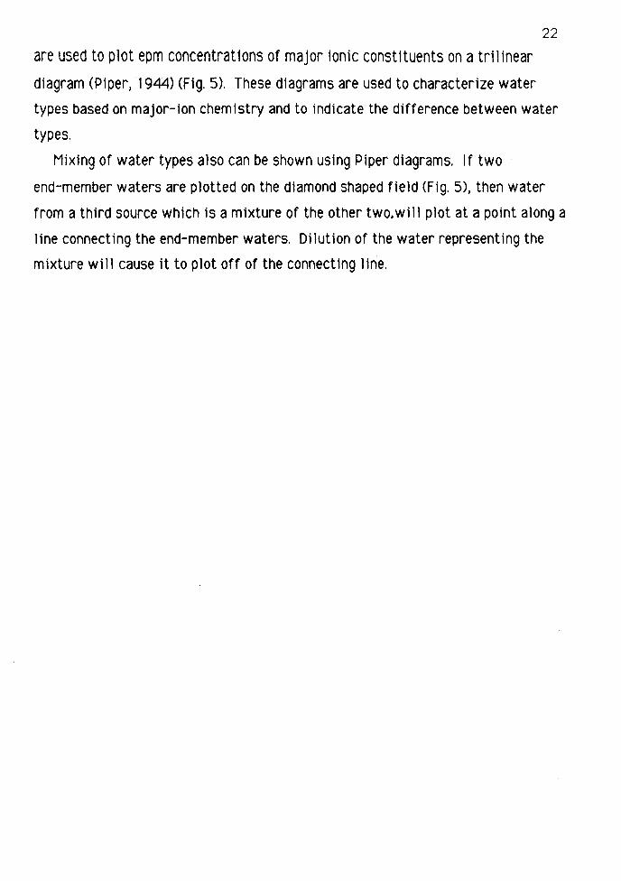
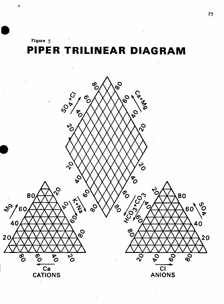
are used to plot epm concentrattons of major 1on1c const1tuents on a tr111near

diagram (Piper, 1944) ffig. 5). These diagrams are used to characterize water

types based on major-ion chemistry and to indicate the difference between water

types.

Mixing of water types also can be shown using Piper diagrams. If two

end-member waters are plotted on the diamond shaped field <Fig. 5), then water

from a third source which is a mixture of the other two. will plot at a point along a

line connecting the end-member waters. Dilution of the water representing the

mixture will cause it to plot off of the connecting llne.

•

•

•

•

Figure 5

PIPER TRILINEAR DIAGRAM

~ CS(, so ~ Ca

CATIONS

A---tt---¥~~ 6 0 '\';

A--.~t'-if'-t-""'"'1-~ 4 0

~ ~ ~ ~ Cl

ANIONS

23

24

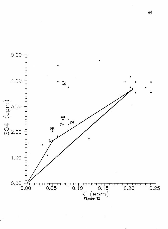
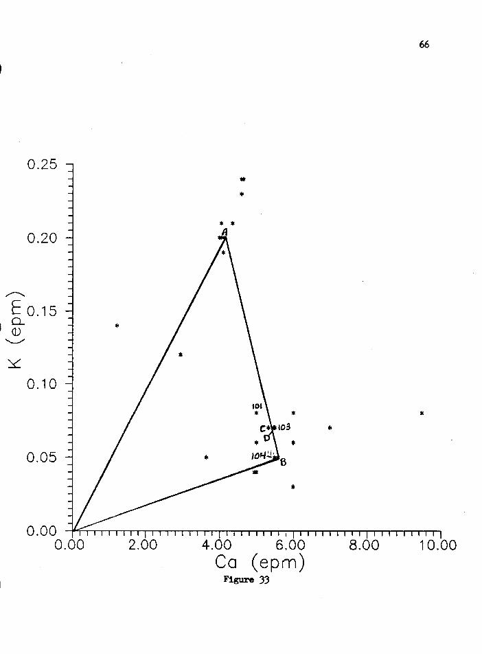
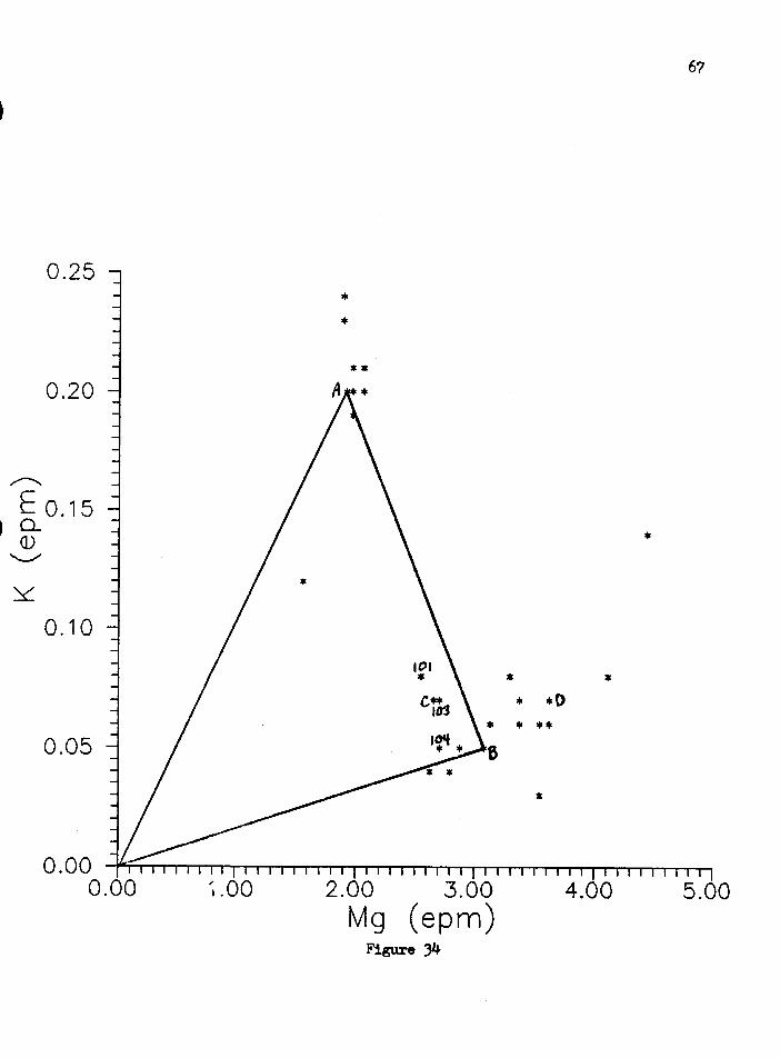
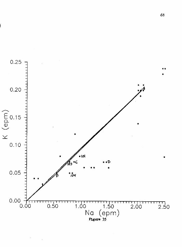
. Mixing Diagrams

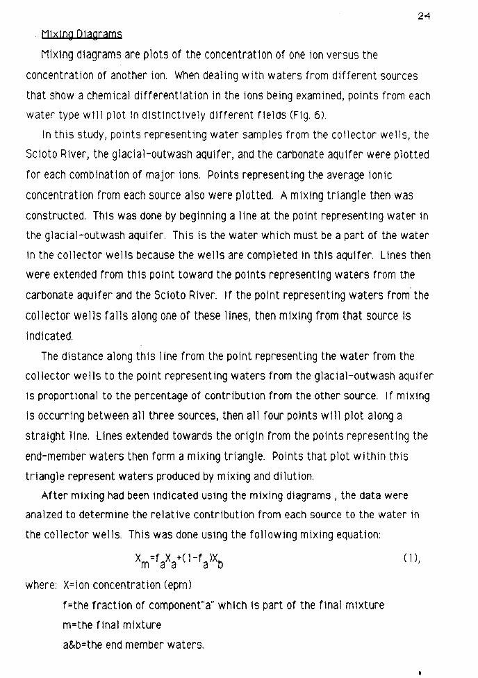
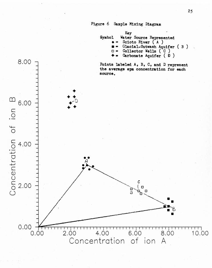
Mixing diagrams are plots of the concentration of one ion versus the

concentration of another ion. When dealing with waters from different sources

that show a chemical differentiation in the ions being examined, points from each

water type w11l plot 1n d1st1nct1ve1y different f1elds CF1g. 6).

In this study, points representing water samples from the collector wells, the

Scioto River, the glacial-outwash aquifer, and the carbonate aquifer were plotted

for each combination of major ions. Points representing the average ionic

concentration from each source also were plotted. A mixing triangle then was

constructed. This was done by beginning a 1 ine at the point representing water in

the glacial-outwash aquifer. This is the water which must be a part of the water

in the collector wells because the wells are completed in this aquifer. Lines then

were extended from th1s point toward the po1nts represent tng waters from the

carbonate aquifer and the Scioto River. If the point representing waters from the

collector wells falls along one of these lines, then mixing from that source is

indicated.

The distance along this line from the point representing the water from the

collector wells to the point representing waters from the glacial-outwash aquifer

is proportional to the percentage of contribution from the other source. If mixing

is occurring between all three sources, then all four points will plot along a

straight line. Lines extended towards the origin from the points representing the

end-member waters then form a mixing triangle. Points that plot within this

triangle represent waters produced by mixing and dilution.

After mixing had been indicated using the mixing diagrams , the data were

aoalzed to determine the relative contribution from each source to the water in

the collector wells. This was done using the following mixing equation:

Xm=faXa+(l-fa)Xb (1),

where: X=ion concentration Cepm)

f=the fraction of component"a" which ls part of the final mixture

m=the final mixture

a&b=the end member waters.

8.00

OJ 6.00 c 0

4-0

c 0 4.00

_µ

0 L

_µ

c . Q)

u c 0 2.00 u

0.00 0.00

• •• .,-D

••

Figure 6 Sample Mixing Diagram

Key ·iymbol Water Source Represented

• • Scioto River ( A ) • • Glacial-Outwash Aquifer ( B ) o • Collector Wells ( C ) + • ~rbonate Aquifer ( D )

Points labeled A, B, C, and D represent the average epm concentration for each source •

2.00 4.00 6.00

of 8.00

A Concentration . ion

25

10.00

Rearrangement of th1s formula to solve for fa yields the following equation:

(2).

Analysis of all major ions for which mixing is indicated using the average ionic

concentrations (Table 7) will produce a range of values for the contribution to the

collector well waters from each source.

27

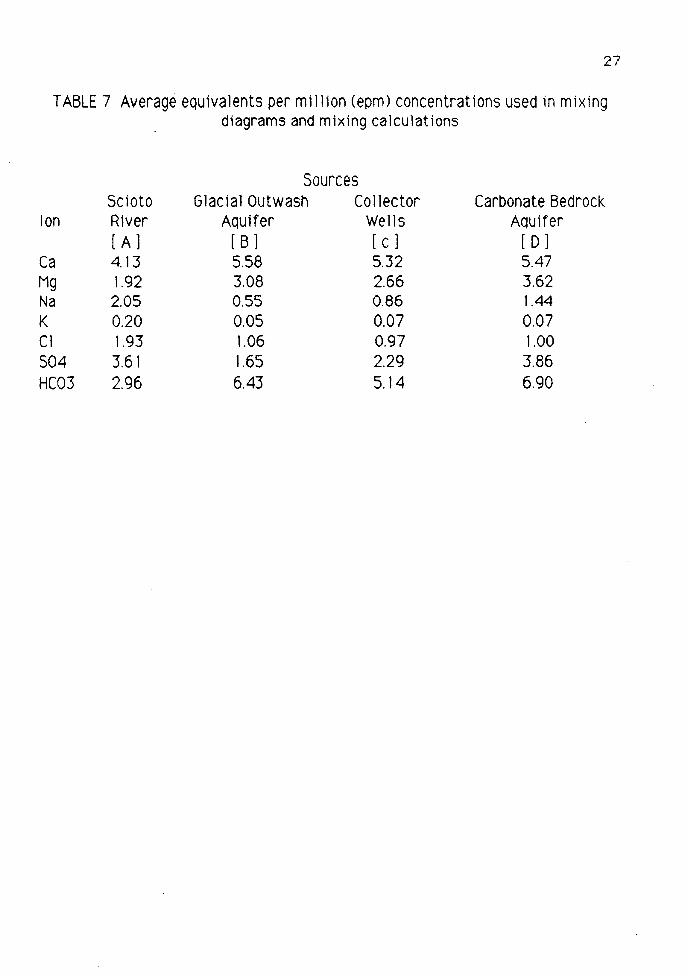
TABLE 7 Average equivalents per million (epm) concentrations used in mixing diagrams and mixing calculations

Sources Scioto Glacial Outwash Collector Carbonate Bedrock

Ion River Aquifer Wells Aquifer [ A ] [ B ] [ c ] [ D ]

Ca 4.13 5.58 5.32 5.47 Mg 1.92 3.08 2.66 3.62 Na 2.05 0.55 0.86 1.44 K 0.20 0.05 0.07 0.07 Cl 1.93 1.06 0.97 1.00 504 3.61 1.65 2.29 3.86 HC03 2.96 6.43 5.14 6.90

28

Varjatjons jo lonjc Concentrations jo Water From the Scioto R1yer

Graphs of ionic concentration versus river water temperature and versus r1ver

stage from the Scioto River also were constructed. These plots were made to

identify trends in changes in ionic concentrations due to changes in these two

factors. If 1on1c concentrat1ons do vary systemat1cally, then changes 1n water

quality can be anticipated during times when induced stream infiltration is higher

or lower.

It was my initial intent to determine if the trends in variation of ionic

concentrations from the river due to changes 1n water temperature and river stage

were reflected in the collector-well samples and to try to analyze variations in

contributions from the river with the changes in river stage and temperature. I

was not able to do th1s because or an 1nsurnc1ent amount or water qual 1ty data

from the collector wells at different seasons of the year.

R1ver stage was examined as a functton of r1ver d1scharge from records taken

at the Jackson Pike Sewage Treatment Plant.

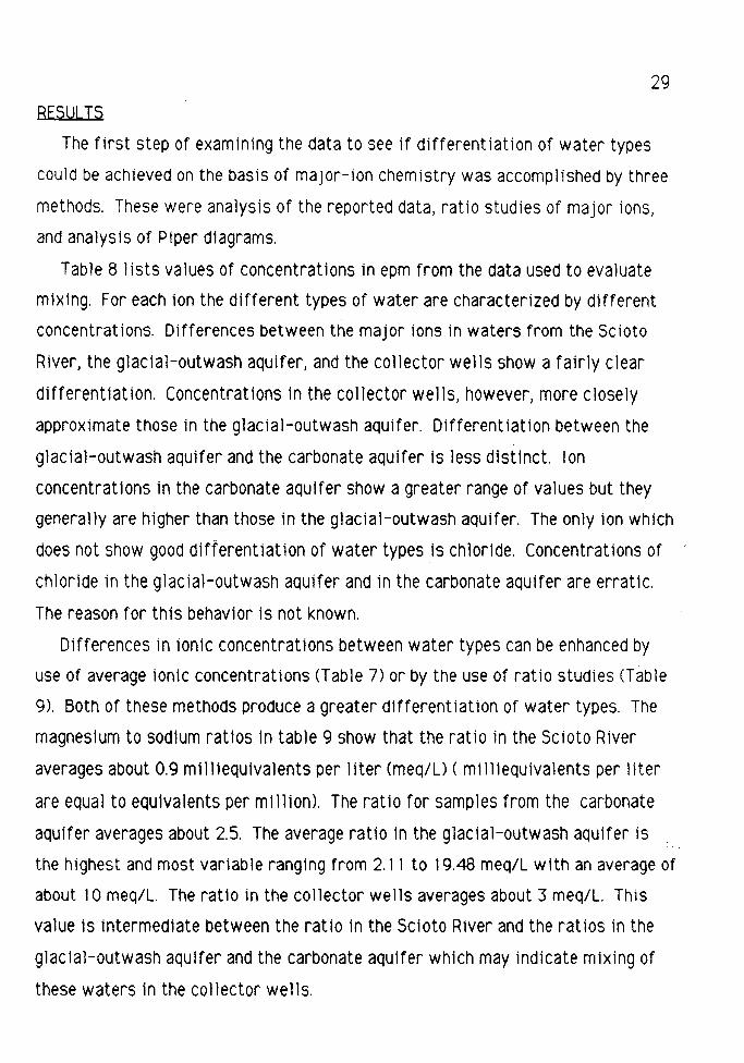
29

RESULTS

The first step of examining the data to see if differentiation of water types

could be achieved on the basis of maJor-ion chemistry was accomplished by three

methods. These were analysis of the reported data, ratio studies of major ions,

and analysis of Piper diagrams.

Table 8 lists values of concentrations in epm from the data used to evaluate

mixing. For each ion the different types of water are characterized by different

concentrations. Differences between the major ions in waters from the Scioto

River, the glacial-outwash aquifer, and the collector wells show a fairly clear

differentiation. Concentrations in the collector wells, however, more closely

approximate those in the glacial-outwash aquifer. Differentiation between the

glacial-outwash aquifer and the carbonate aquifer is less d1st1nct. Ion

concentrations in the carbonate aquifer show a greater range of values but they

generally are higher than those in the glacial-outwash aquifer. The only ion which

does not show good differentiation of water types is chloride. Concentrations of

chloride in the glacial-outwash aquifer and in the carbonate aquifer are erratic.

The reason for this behavior is not known.

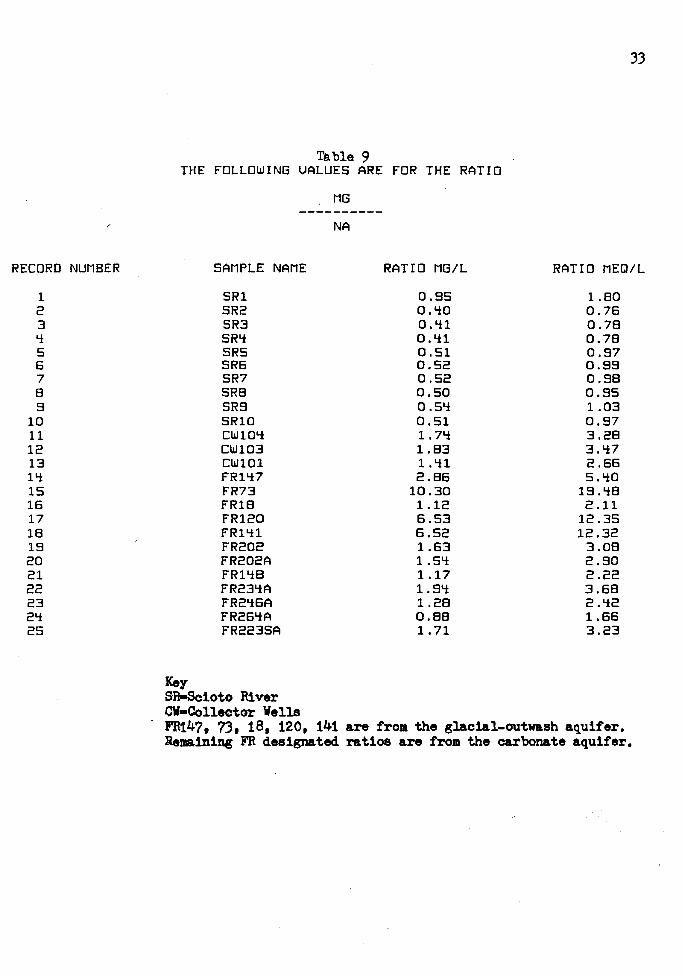
Differences in ionic concentrations between water types can be enhanced by

use of average ionic concentrations (Table 7) or by the use of ratio studies CTable

9). Both of these methods produce a greater differentiation of water types. The

magnesium to sodium ratios In table 9 show that the ratio in the Scioto River

averages about 0.9 milliequivalents per liter <meq/U < milliequivalents per liter

are equal to equivalents per mlllion). The ratio for samples from the carbonate

aquifer averages about 2.5. The average ratio in the glacial-outwash aquifer is

the highest and most variable ranging from 2.11 to 19.48 meq/L with an average of

about 1 O meq/L. The ratio in the collector wells averages about 3 meq/L. This

value is intermediate between the ratio in the Scioto River and the ratios in the

glaclal-outwash aquifer and the carbonate aquifer which may indicate mixing of

these waters in the collector wells.

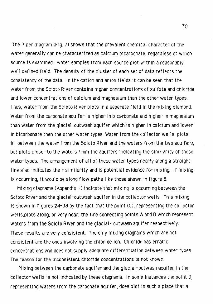
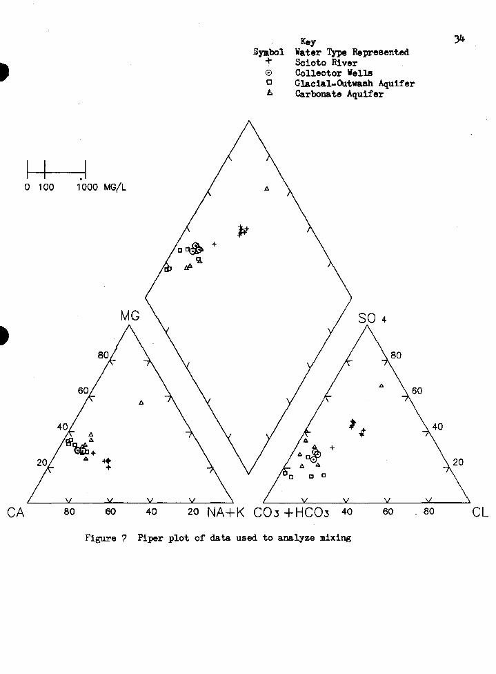
The Piper diagram <Fig. 7) shows that the prevalent chemical character of the

water generally can be characterized as calcium bicarbonate, regardless of which

source is examined. Water samples from each source plot within a reasonably

well defined field. The density of the cluster of each set of data reflects the

consistency of the data. In the cation and anion fields it can be seen that the

water from the Scioto River contains higher concentrations of sulfate and chloride

and lower concentrations of calcium and magnesium than the other water types.

Thus, water from the Scioto River plots in a seperate field in the mixing diamond.

Water from the carbonate aquifer is higher in bicarbonate and higher in magnesium

than water from the glacial-outwash aquifer which is higher in calcium and lower

1n bicarbonate then the other water types. Water from the collector wells plots

in between the water from the Scioto River and the waters from the two aquifers,

but plots closer to the waters from the aquifers indicating the similarity of these

water types. The arrangement of all of these water types nearly along a straight

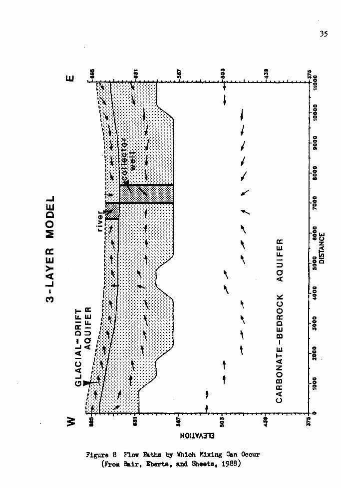
line also indicates their similarity and is potential evidence for mixing. If mixing

is occurring, it would be along flow paths like those shown in figure 8.

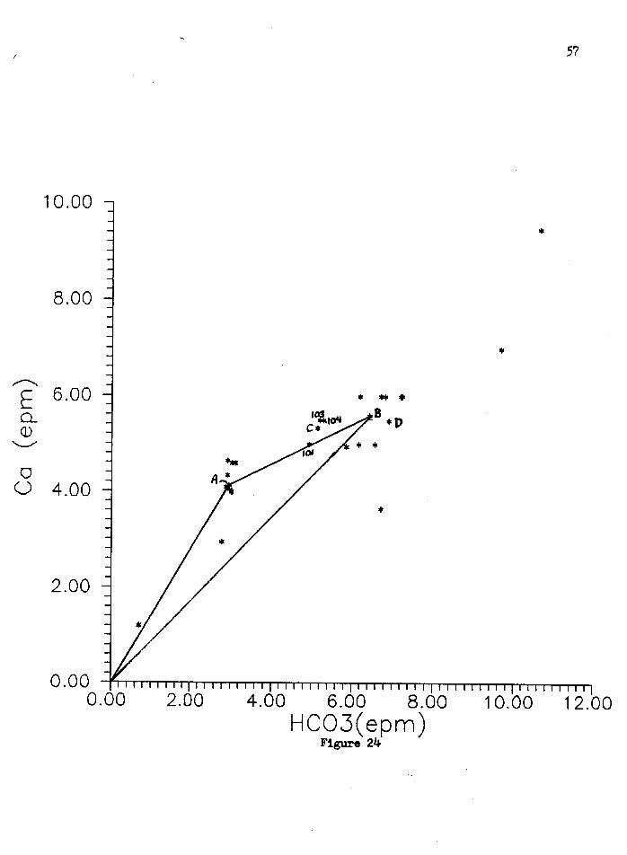
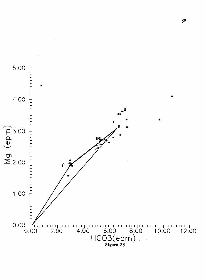
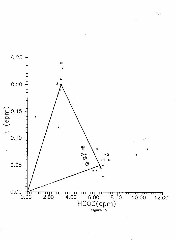
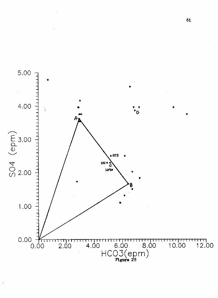
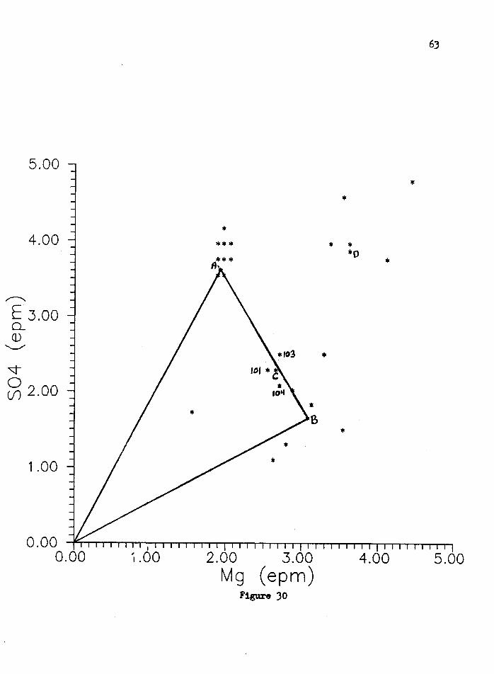
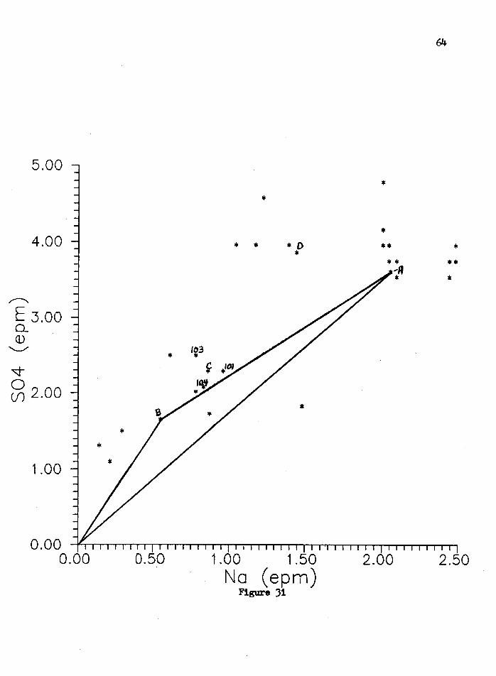
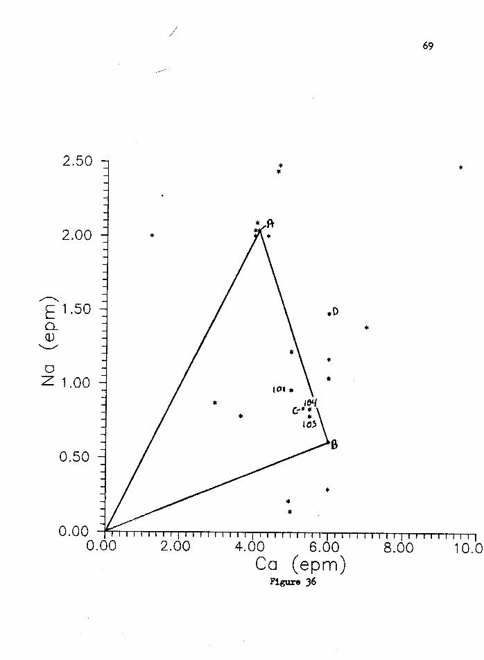
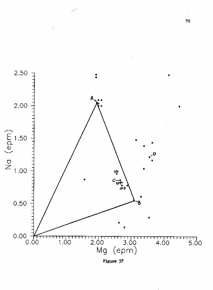
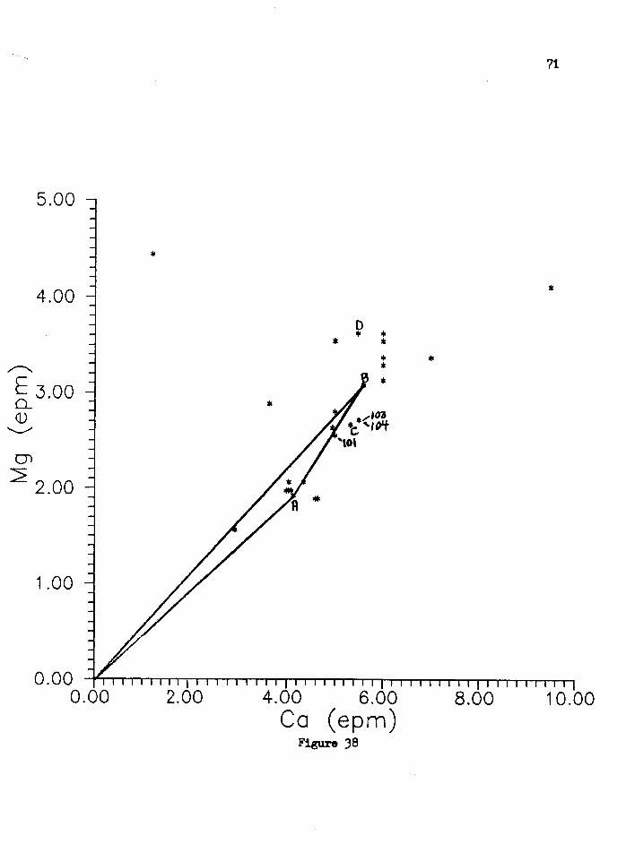
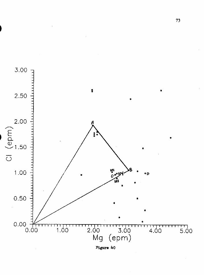
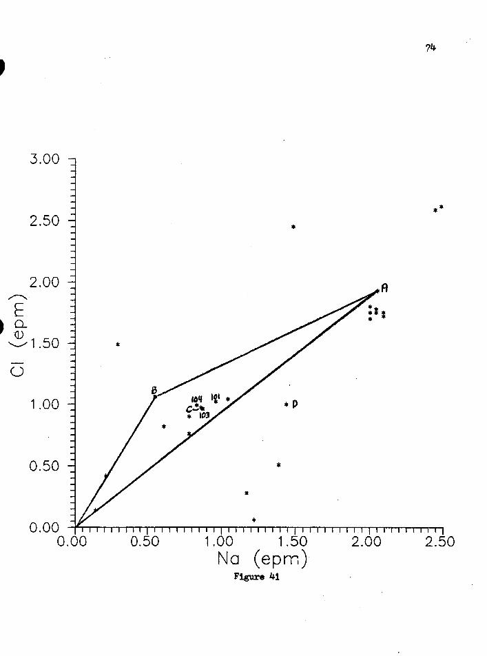
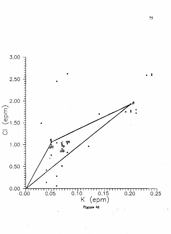
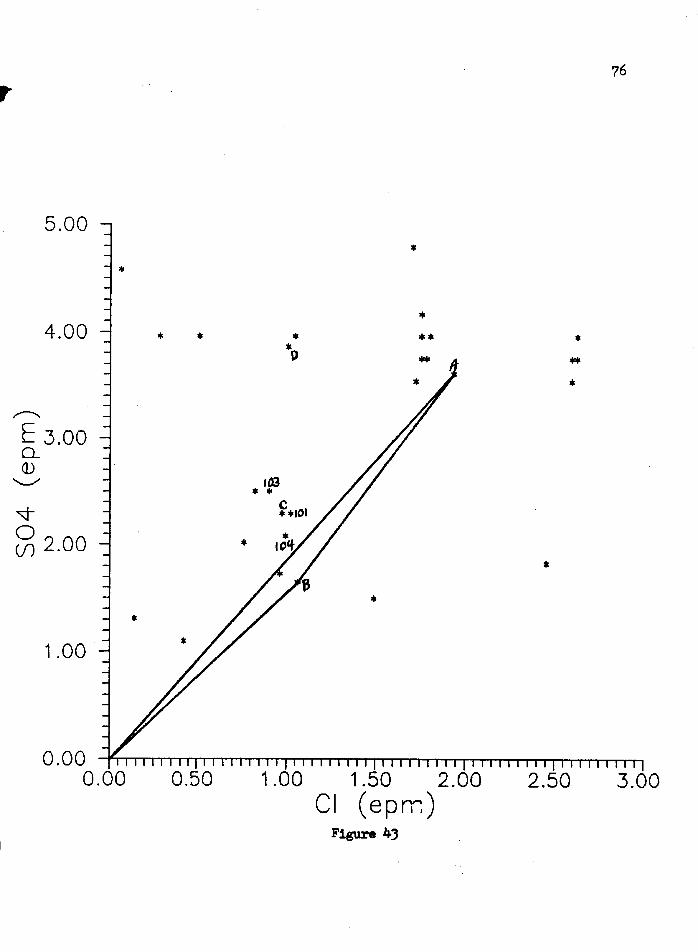
Mixing diagrams (Appendix 1) indicate that mixing is occurring between the

Scioto River and the glacial-outwash aquifer in the collector wells. This mixing

1s shown 1n figures 24-38 by the fact that the point (C), represent1ng the collector

wells,plots along, or very near, the line connecting points A and B which represent

waters from the Scioto River and the glacial- outwash aquifer respectively.

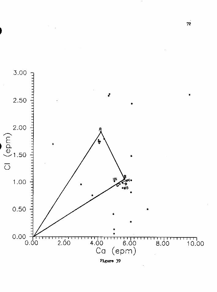
These results are very consistent. The only mixing diagrams which are not

consistent are the ones involving the chloride Ion. Chloride has erratic

concentrations and does not supply adequate differentiation between water types.

The reason for the inconsistent chloride concentrations is not known.

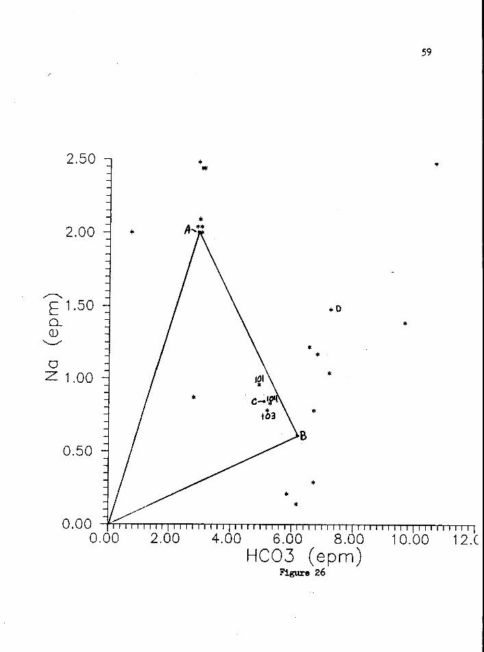
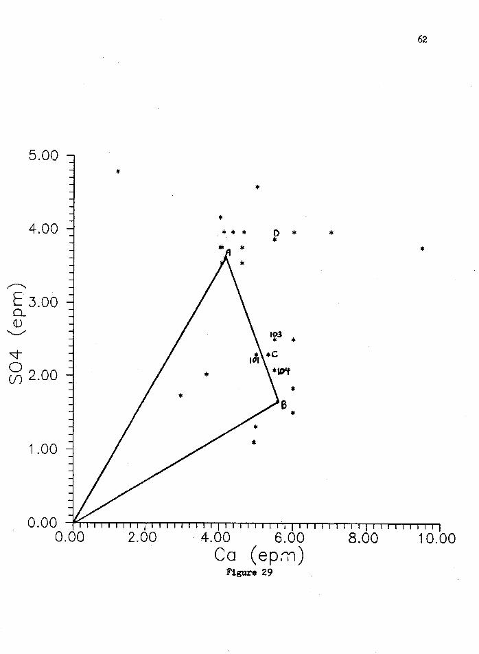
Mixing between the carbonate aquifer and the glacial-outwash aquifer in the

collector wells ls not indicated by these diagrams. In some Instances the point D,

representing waters from the carbonate aquifer, does plot in such a place that a

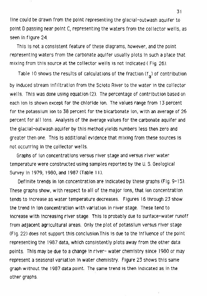
31

line could be drawn from the point representing the glacial-outwash aquifer to

point D passing near point C, representing the waters from the collector wells, as

seen in figure 24.

This is not a cons1stent feature of these d1agrams, however, and the point

represent1ng waters from the carbonate aqu1fer usually plots 1n such a place that

mixing from this source at the collector wells is not indicated (Fig. 26).

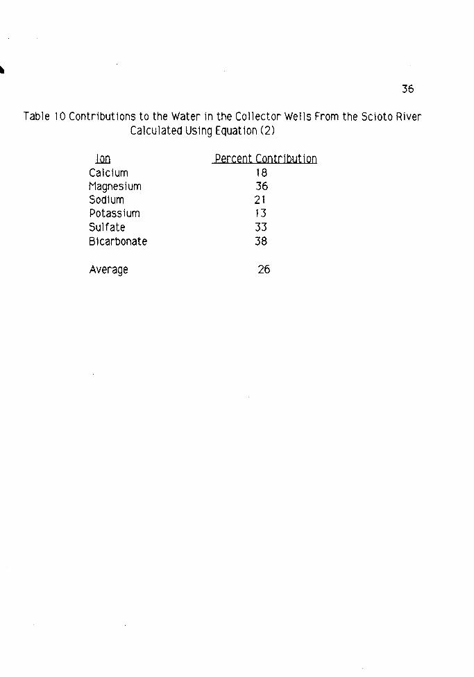
Table 1 O shows the results of calculations of the fraction (fa) of contribution

by induced stream infiltration from the Scioto River to the water in the collector

wells. This was done using equation (2). The percentage of contribution based on

each ion is shown except for the chloride ion. The values range from 13 percent

for the potassium ion to 38 percent for the bicarbonate ion, with an average of 26

percent for all ions. Analysis of the average values for the carbonate aquifer and

the glactal-outwash aquifer by th1s method yields numbers less then zero and

greater then one. Th1s is additional evidence that mixing from these sources is

not occurring tn the collector wells.

Graphs of ion concentrations versus river stage and versus river water

temperature were constructed using samples reported by the U. S. Geological

Survey in 1979, 1980, and 1987 <Table 11 ).

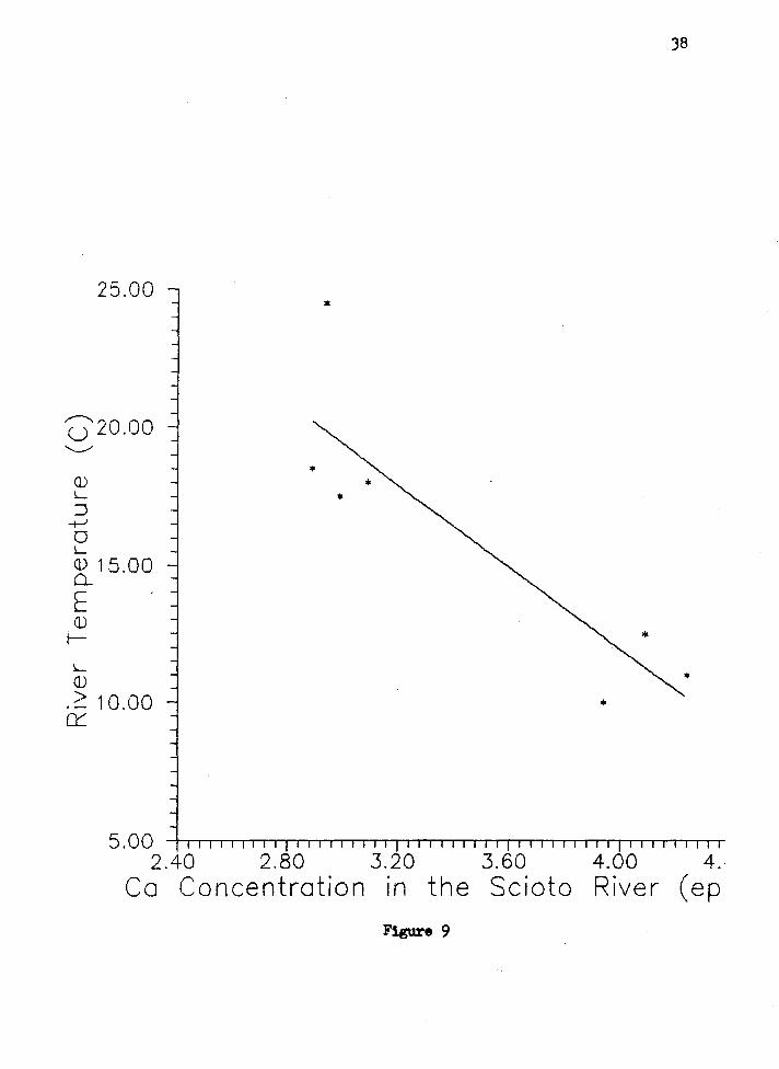
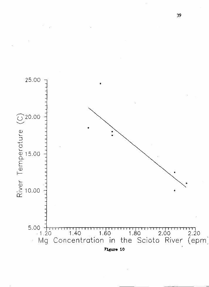
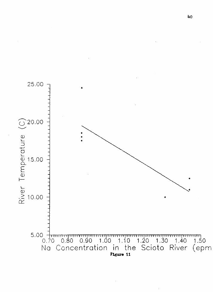
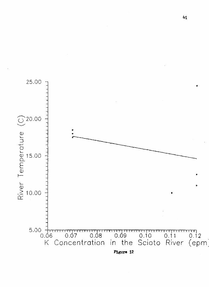
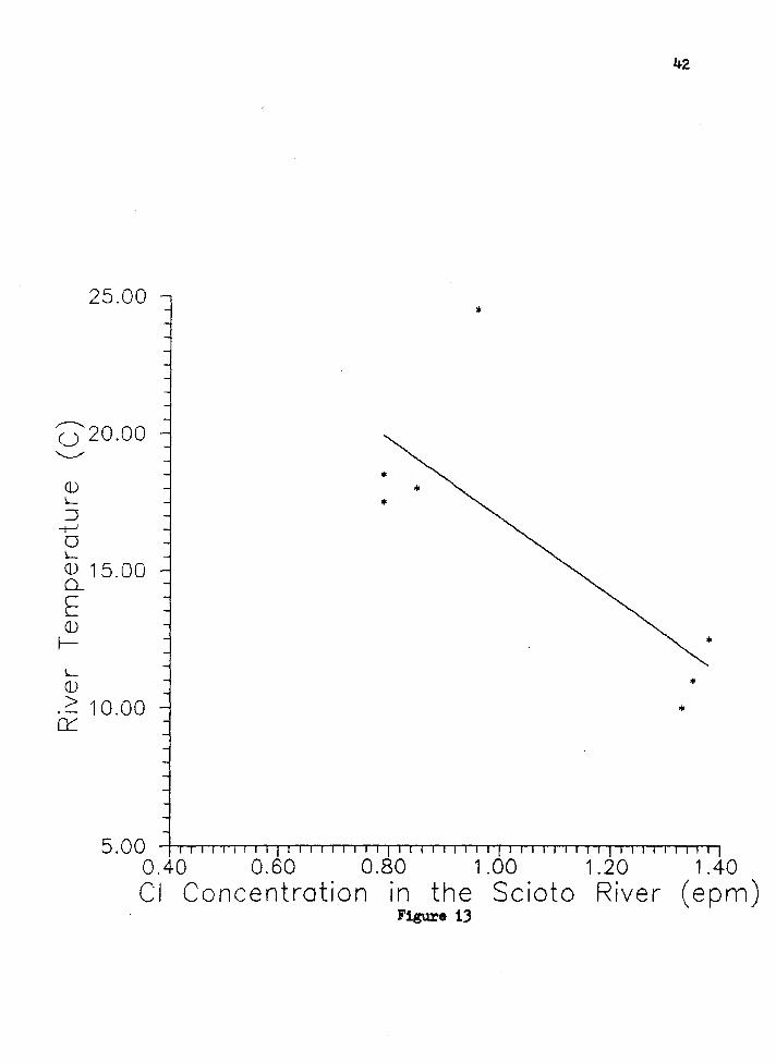
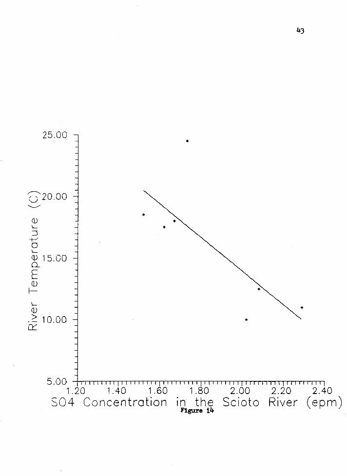
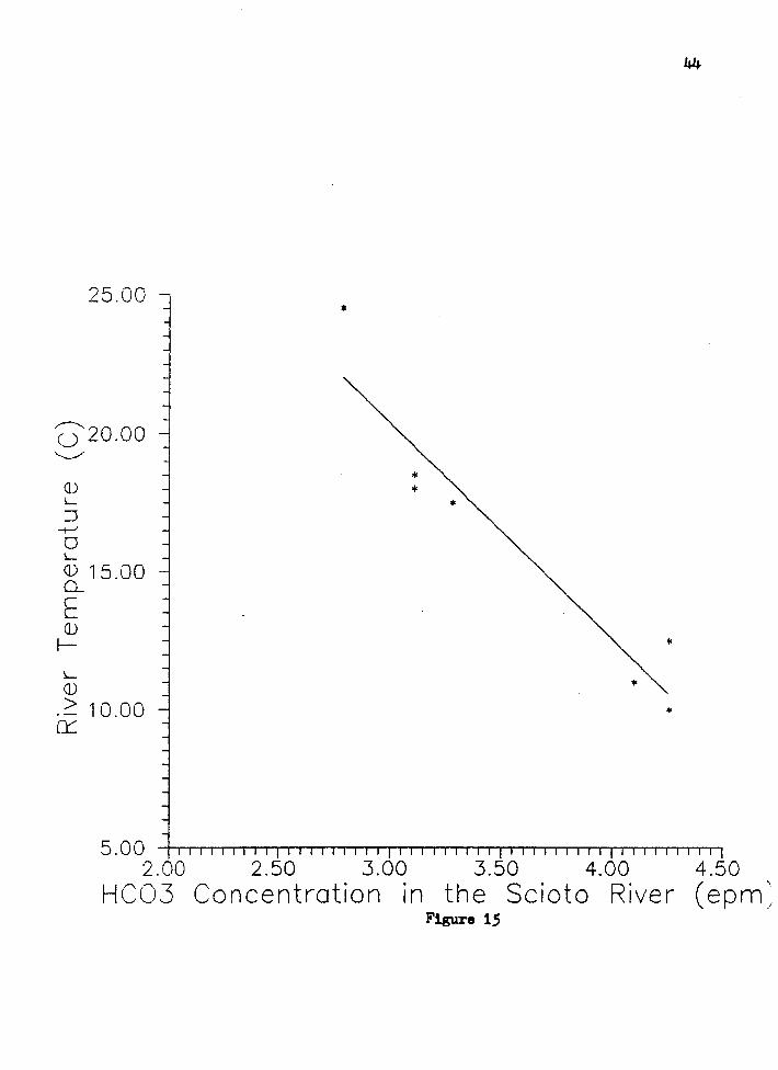
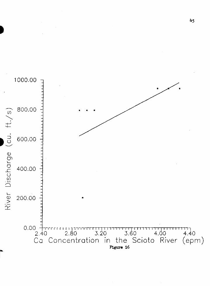
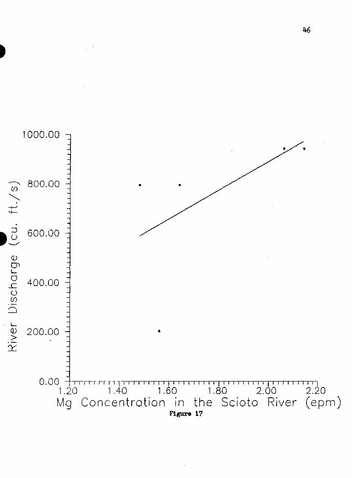
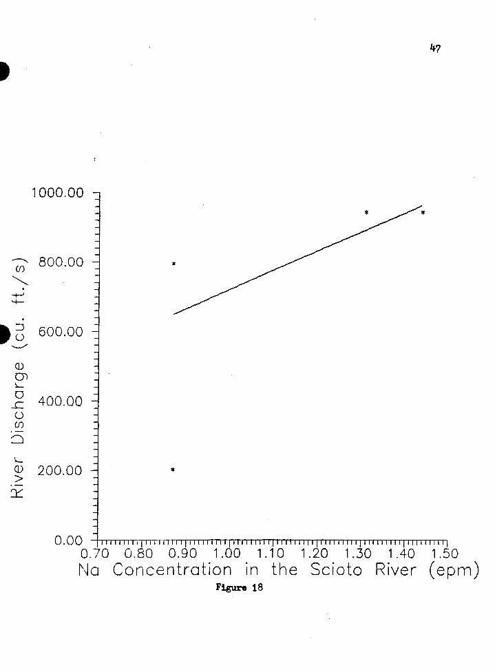
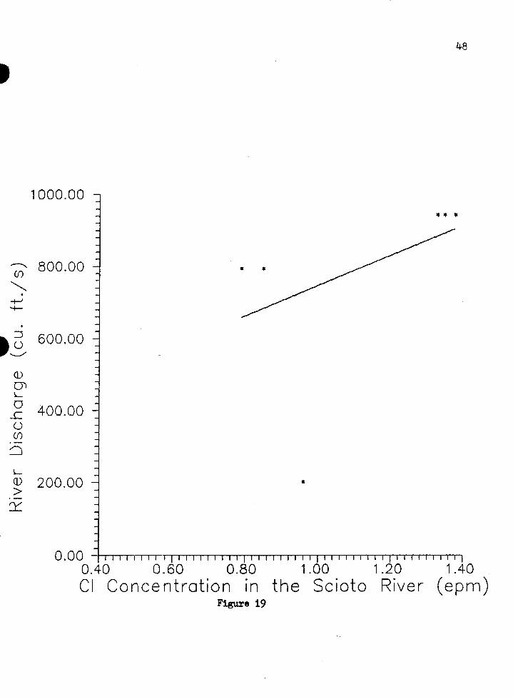
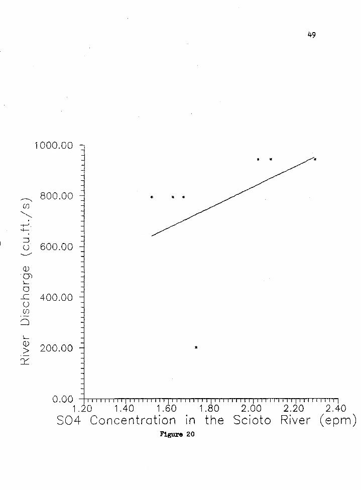
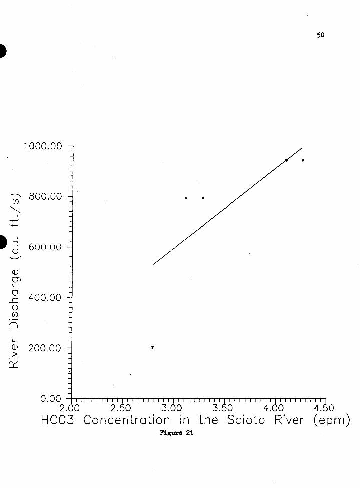
Definite trends in ion concentration are indicated by these graphs <Fig. 9-15).

These graphs show, with respect to all of the major ions, that Jon concentration

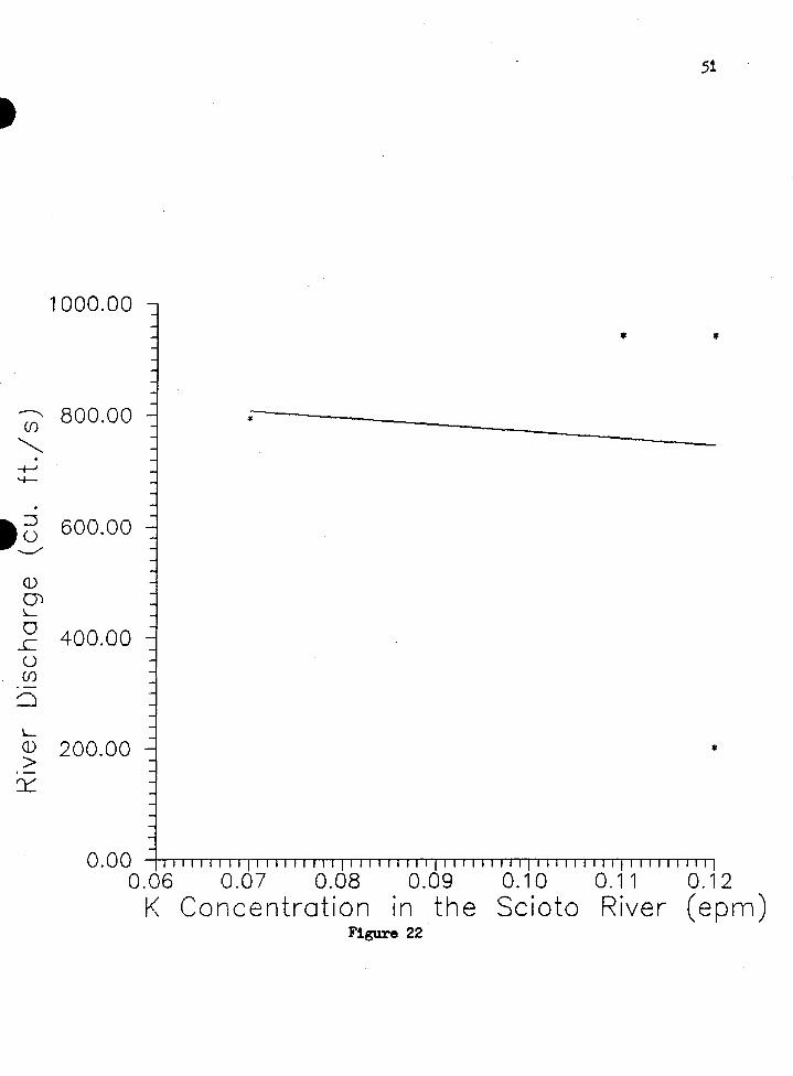
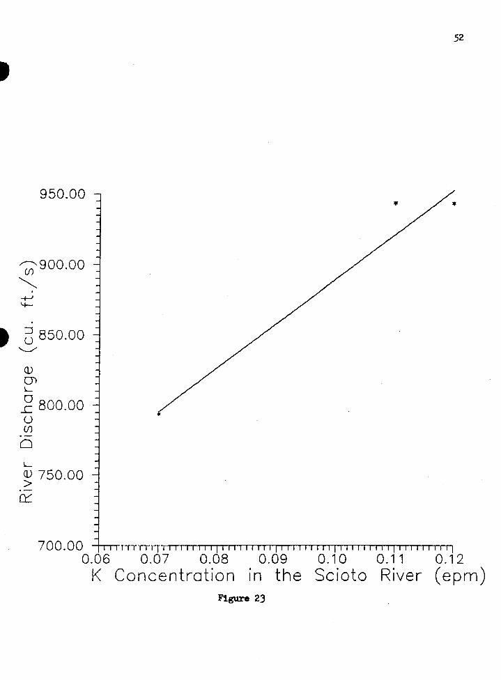
tends to increase as water temperature decreases. Figures 16 through 23 show

the trend 1n ion concentrat1on with variation in river stage. These tend to

1ncrease w1th 1ncreas1ng r1ver stage. Th1s ts probably due to surface-water runoff

from adjacent agricultural areas. Only the plot of potass1um versus r1ver stage

<Fig. 22) does not support this conclusion.Th1s is due to the influence of the point

representing the 1987 data, which consistently plots away from the other data

points. This may be due to a change in river- water chemistry since 1980 or may

represent a seasonal variation in water chemistry. Figure 23 shows this same

graph without the 1987 data point. The same trend is then indicated as in the

other graphs.

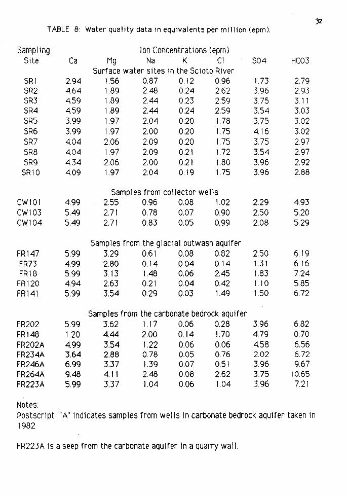
J2 TABLE 8: Water qua! ity data in equivalents per mi 11 ion (epm ).

Sampling Ion Concentrations (epm) Site Ca Mg Na K C1 S04 HC03

Surface water sites in the Scioto River SRl 2.94 1.56 0.87 0.12 0.96 1.73 2.79 SR2 4.64 1.89 2.48 0.24 2.62 3.96 2.93 SR3 4.59 1.89 2.44 0.23 2.59 3.75 3.11 SR4 4.59 1.89 2.44 0.24 2.59 3.54 3.03 SR5 3.99 1.97 2.04 0.20 1.78 3.75 3.02 SR6 3.99 1.97 2.00 0.20 1.75 4.16 3.02 SR7 4.04 2.06 2.09 0.20 1.75 3.75 2.97 SR8 4.04 1.97 2.09 0.21 1.72 3.54 2.97 SR9 4.34 2.06 2.00 0.21 1.80 3.96 2.92

SR10 4.09 1.97 2.04 0.19 1.75 3.96 2.88

Samples from collector wells CW101 4.99 2.55 0.96 0.08 1.02 2.29 4.93 CW103 5.49 2.71 0.78 0.07 0.90 2.50 5.20 CW104 5.49 2.71 0.83 0.05 0.99 2.08 5.29

Samples from the glacial outwash aquifer FR147 5.99 3.29 0.61 0.08 0.82 2.50 6.19 FR73 4.99 2.80 0.14 0.04 0.14 1.31 6.16 FR18 5.99 3.13 1.48 0.06 2.45 1.83 7.24

FR120 4.94 2.63 0.21 0.04 0.42 1.10 5.85 FR141 5.99 3.54 0.29 0.03 1.49 1.50 6.72

Samples from the carbonate bedrock aquifer FR202 5.99 3.62 1.17 0.06 0.28 3.96 6.82 FR148 1.20 4.44 2.00 0.14 1.70 4.79 0.70 FR202A 4.99 3.54 1.22 0.06 0.06 4.58 6.56 FR234A 3.64 2.88 0.78 0.05 0.76 2.02 6.72 FR246A 6.99 3.37 1.39 0.07 0.51 3.96 9.67 FR264A 9.48 4. 11 2.48 0.08 2.62 3.75 10.65 FR223A 5.99 3.37 1.04 0.06 1.04 3.96 7.21

Notes: Postscript "A" indicates samples from wells in carbonate bedrock aquifer taken in 1982

FR223A 1s a seep from the carbonate aquifer 1n a quarry wall.

RECORD NUMBER

1 2 3 'i 5 6 7 8 9

10 11 12 13 1 'i 15 16 17 18 19 20 21 22 23 2'i 25

Table 9 THE FOLLOWING UALUES ARE

MG ----------

SAMPLE NAME

SRl SR2 SR3 SR'i SR5 SR6 SR7 SR8 SR9 SRlO CWlO'i CW103 CW101 FR1'i7 FR73 FR18 FR120 FRl'il FR202 FR202A FRl'iB FR23'iA FR2'i6A FR26'i:A FR223SA

Key S·R-Scioto River CW•Collector Wells

NA

33

FOR THE RAT ID

RATIO MG/L RATIO MECJ/L

0.95 1.80 O.'iO 0.76 O.'il 0.78 O.'il 0.78 0.51 0.97 0.52 0.99 0.52 0.98 0.50 0.95 0.5'i 1.03 0.51 0.97 1. 7'i 3.28 1.83 3.'i7 1. 'il 2.66 2.86 5.'iO

10.30 19.'i8 1.12 2.11 6.53 12.35 6.52 12.32 1.63 3.08 l.5'i 2.90 1.17 2.22 l.9'i 3.68 1.28 2.'i2 0.88 1.66 1. 71 3.23

FR147, 73, 18, 120, 141 are from the glacial-outwash aquifer. Remaining FR designated ratios are from the carbonate aquifer.

I I 0 100

CA 80

.1 1000 MG/L

60 40

Ke;r Symbol Water Type Represented

+ Scioto River © Collector Wells a Glacial-Outwash Aquifer I;;. Carbonate Aquifer

20 NA+K COJ +HCOJ 40 60

Figure 7 Piper plot of data used to analyze mixing

- 80 CL

..J w c 0 :E

a: w > <C ..J

I

CW)

w fit ..

0 .,, .,

' ' J

I I I ¥

.......

' \ ' ' ' ~

\

' \ t t

t

~ .., 0 ., .,

NOllVA313

Figure 8 Flow Paths by Which Mixing Oan Occur (From Pair, Eberts, and Sheets, 1988)

3.5

• .,, .., l:;o .....

0 0 --0 0 0 0 -0 0 0 •

0 0 0 • 0 0

:?

0 0 I.I.I

a: a CJ z

llJ ~ u. o-::::> gc 0

.,, <t

0 0

~ 0 .. (J

0 a: 0 c 0

0 llJ .., m I

llJ 0 0

I- 0

<t " z 0

0 m 0 a: 0 -<t (J

0

• E .., ~

36

Table 1 o Contributions to the Water in the Collector Wells From the Scioto River Calculated Using Equation (2)

Calcium Magnesium Sodium Potassium Sulfate Bicarbonate

Average

Percent Cootrjbutjoo 18 36 21 13 33 38

26

37

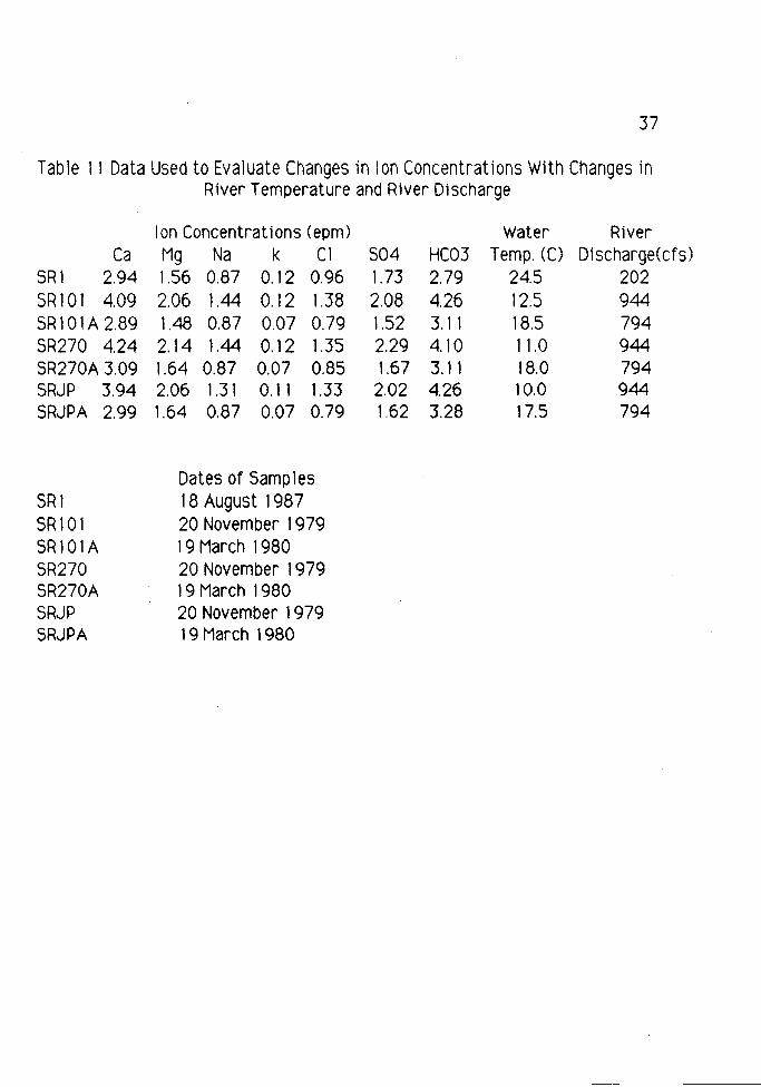
Table 11 Data Used to Evaluate Changes in Ion Concentrations With Changes in River Temperature and River Discharge

Ca SR1 2.94 SR101 4.09 SR101A 2.89 SR270 4.24 SR270A 3.09 SRJP 3.94 SRJPA 2.99

SRl SR101 SR101A SR270 SR270A SRJP SRJPA

I on Concentrat i ens ( epm) Mg Na k Cl 1.56 0.87 0.12 0.96 2.06 1.44 0.12 1.38 1.48 0.87 0.07 0.79 2.14 1.44 0.12 1.35 1.64 0.87 0.07 0.85 2.06 1.31 0.11 1.33 1.64 0.87 0.07 0.79

Dates of Samples 18 August 1987 20 November 1979 1 9 March 1980 20 November 1 979 1 9 March 1 980 20 November 1 979 1 9 March 1980

504 1.73 2.08 1.52 2.29 1.67 2.02 1.62

HC03 2.79 4.26 3.11 4.10 3. 11 4.26 3.28

Water Temp. (C)

24.5 12.5 18.5 11.0 18.0 10.0 17.5

River Discharge(cfs)

202 944 794 944 794 944 794

38

25.00 *

(]20.00 '-...,...../

* Q) * !........ * :J -+-' 0 !........

Q) 1 5.00 Q_

E Q)

I-

!........ Q)

.> 10.00 ... er:

5.00 -1-T-~-r-r-~ .............. ..........-,--,--,-~..-r-T" .............. -.-.-,--,--,--..-.-,....,....,...............,-r-r-..-.-r-..-r-~ 2.40 2.80 3.20 3.60 4.00 4.·

Co Concentration in the Scioto River (ep

Figure 9

25.00

u20.oo

(1) L

:J -+--' 0 L

()) 15.00 0...

E Q)

~

L ())

.> 10.00 er:

39

*

* ...

5 . 0 0 -+-.--~..,..........,.-.--.-.--.-.-.....-.--r~--.-.-...-.-......-.-,.-.-.-.........-.-...,_,......,....,.....,.....___.........-.-~-.-.-.......-.

. 1 .20 1.40 1.60 1.80 2.00 2.20 tv1g Concentration in the Scioto River (epm~

Figure 10

25.00

,.--...._ u 20.00

Q) L

:::J -+-' 0 L

(1) 15.00 Q_ .

E Q)

I-

L Q)

.> 10.00 er:

40

*

•

5. 00 -j....,...,...~...,......,,..,.,....,...,...,~.._,....,...,...,....,...,....~...,....,....,..,....,....,...~..,...,...,.,..~ .............................. ............-.-.-.-.-.-............... ~

0.70 0.80 0.90 1.00 1.10 1.20 1.30 1.40 1.50 Na Concentration in the Scioto River (epm

Figure 11

41

25.00 *

()20.00 '-__./

... (}) ... I._

:J -t-J 0 I._

Q) 15.00 Q_

E Q)

f-I._

Q) ...

.> 10.00 ... er:

5.00 -h-~.....-.-.......,....,,......,...,~~_,...,..,.-,-r-r..........,...,.-.-.-.,-r-r....-.-r...-r-r-r-.-r~..-.-.-..-.-.-..-.-.....,-,.-,-,

0.06 0.07 0.08 0.09 0.10 0.11 0.12 K Concentration in the Scioto River (epm~

Figure 12

25.00

_,,---....., u 20.00

Q) L ::J

-+--' 0 L

Q) 15.00 Q_

E Q)

f-

L Q)

.> 10.00 er::

42

*

...

5. 0 0 -+---.......-.-....-.--.-~---.-.-~~........-T"",_.,........,.....,...,......,~~~,....,......,..,_.,........,........,_..._,_,........-.--.-.

1.00 1 .20 1 .40 0.40 0.60 0.80 Cl Concentration 1n the Scioto River (epm)

Figure 13

25.00

()20.00

CD L

:::J -t-.J 0 L

(}) 1 5.00 Q_

E Q) I-

L (})

.> 10.00 CL

43

*

*

*

5 . 0 0 -+-i-~c-r-r-r-r-r-r""T"""T"T'"T"'T""T"-r-r-r".,....,.....,.-....-r-r-T"'T-i-,....,........,-r-r'T~..,....,.....,...,.....,.....,.,.......,.....'T'"T""T""r'T""'l-",.............."-r-1

1 .20 1 .40 1 .60 1 .80 2.00 2.20 2.40 S04 Concentration in the Scioto River (epm)

Figure 14

44

25.00 *

~

(__) 20.00 "-.--''

Q) L

:J +-' 0 L

Q) 15.00 Q_

E Q)

~ * L Q) *

.> 10.00 * er:

5. 0 0 ~~-.-.-.-.....-.-.~.,.......,..... ............... --.--.-~~.....-.-...............-..-.-.-............... --.--.-~~~~ 2.00 2.50 3.00 3.50 4.00 4.50

HC03 Concentration 1n the Scioto River (epm~ Figure 1.5

1000.00

,.--.__ 800.00 ())

"-... . -+--' '+---

. t~ 600.00

Q)

CJ) L

0 400.00 _c u ()) ·-~

L (1)

> 200.00 *

·-'.J:::

0.00 1 1 TTTTTlTl I I I I I I I I I I I I I I I I I I I I I I I I I I I I I I I I I I I I I I 1

2.40 2.80 3.20 3.60 4.00 4.40 Co Concentration in the Scioto River (epm)

Figure 16

46

1000.00

~ 800.00 ([)

"--. -+-' '+--

. t~ 600.00

Q)

O'> !......

0 400.00 ....c u ([) ·-~

!...... (])

> 200.00 *

·-:r::

0. 00 rrr n n -,-, f I I I I I I I I I I I I I I I I I I I I I I I I I I I I I I I I I I I I I I

1 .20 1 .40 1. 60 1.80 2.00 2.20 Mg Concentration in the Scioto River (epm)

Figure 17

47

1000.00

-...._ 800.00 ())

"'--. +..J '+--

. tG 600.00

....__/

Q) Q) L

0 400.00 ...c u ()) ·-:::J

L Q) 200.00 * > ·-

'.J::::

0. 0 Q T1TTJTTIT I I I I 1 I I I I I I I I 11 I I I I I I I I 11 I I I I I I I I 11 I I I I I 11 I 11 I I I I I I I I 11 I I I I I I I I j

0. 70 0.80 0.90 1.00 1.10 1 .20 1 .30 1 .40 1 .50 Na Concentration in the Scioto River (epm)

Figure 18

48

1000.00

* * •

....--.._, 800.00 CJ)

"" . -+-' '+-

. t~ 600.00

Q)

O'l L

0 400.00 _c u CJ) ·-'.'.:)

L Q) 200.00 * > ·-

J::::

0.00 Tl I I I I 11 I I I 11 I I I I I I I I 111 I I I I I I I 11 I I I I I I I I I 0.40 0_60 0.80 1 .00 1 .20 1.40 Cl Concentration in the Scioto River (epm)

Figure 19

...--..,. (f)

................ . -;-> -+-. ~ u

-....../

Q)

Ul L

0 _c u (/)

CJ

L Q)

> ·-~

49

1000.00

800.00

600.00

400.00

200.00 *

0 . 0 0 -+--r-,~..,.........,..T""r"T'"" .............. -.-.--r"T"""T""T'""T""r"T'"",........,....,-r-T'""l"-.-.-.-..-..-r-..........,........,....,.............-r..-r-.-....,...,....,.""T'""T""T"........--.

1 .20 1 .40 1 .60 1 .80 2.00 2.20 2.40 S04 Concentration in the Scioto River (epm)

Figure 20

.50

1000.00

...---.... 800.00 (/)

"---. +-' '-+--

t:) 0 600.00

..._/

Q) ()) L

0 400.00 _c 0 (/) ·-CJ

L (1)

> 200.00 *

·-:r:::

0 . 0 0 -+-,-..,.......-,-...,.-r-y~l'""""T'""""T""..-r-r-...-r--T--.--.-ir-r-T""..-r-r-.,_......,.-r-r-1r-r-r-..-.--.-"'T""'"""T"""T...,....,.-,--r-.-~T"'""1

2.00 2.50 3.00 3.50 4.00 4.50 HC03 Concentration in the Scioto River (epm)

Figure 21

51

1000.00

• *

..--..,, (/)

800.00 *

"'-. -+-' ~

.

-~ 600.00 '---""

(})

O'l L

0 400.00 ..c u (f) ·-~

L Q)

> 200.00 *

~

0 . 0 0 -+-.-ir-r-T-T-m-......-r-i--T'"T"'T""'1--r-T""T-r-T'"T"~.,.........,...r-r-r-T..........-r~.,...,...,....,~~......--r-r-~--r-r-r-r-r-i

0.06 0.07 0.08 0.09 0.10 0.11 0.12 K Concentration in the Scioto River (epm)

Figure 22

' 950.00

~900.00

"' . +-' 4-

.

.52

t G sso.oo ~

Q) CJ) L

0 _c 800.00 u (/)

0

L

Q) 750.00 >

er:::

700.00 jl 111111111111111 1111111111111111111111111111111111

0.06 0.07 0.08 0.09 0.10 0.11 0.12 K Concentration in the Scioto River (epm)

Figure 23

53

RECOMMENDATIONS FOR FURTHER STUDIES

In order to evaluate temporal variations in the relative contributions of the

potential source waters to the water in the collector wells, a more comprehensive

study including regular sampling and water-quality testing throughout the year

needs to be conducted. This sampling should encompass a wide range of water

temperatures and river stages. A study of the variations in relative contributions

with changes in pumping rate and a study of temporal variations in streambed

permeability would allow all of the relevant factors to be considered to

understand the hydrogeology of the area better.

References Cited

de Roche, J. T., 1985. Hydrogeology and Effects of Landfi l 1s on Ground-Water

Quality, Southern Franklin County, Ohio: U.S. Geological Survey Water

Resources Investigations Report 85-4222, 58p.

54

de Roche, J. T. and A C. Razem, 1984. Water Quality of A Stream-Aquifer System,

Southern Franklin County, Ohio: U. s. Geological Survey Water Resources

Investigations Report 84-4238, 44p.

Eberts, S. M., 1987. Potential Effects of Chemical Spills or Cessation of Quarry

Dewatering on a Municipal Ground-Water Supply, Southern Franklin County,

Ohio: The Ohio State University, Department of Geology and Mineralogy,

Unpublished Master's Thesis, 104p.

Moreno. R. M .. 1988. An Investigation of the Hydraulic Conductivity of the Scioto

River Streambed at the South Well Field, Southern Franklin County, Ohio:

The Ohio State University, Department of Geology and Mineralogy,

Unpublished Senior Thesis, 41p.

Norris, S. E., 1986. Reevaluation of the Stilson Pump Test Data, Unpublished File,

u. S. Geological Survey, Columbus, Ohio.

Schmidt, J. J. and R. S. Goldthwa1t, 1958. The Ground-Water Resources of Franklin

County, Ohio: Ohio Department of Natural Resources Division of Water

Bulletin 30, 97p.

Sheets, R. A., E. s. Bair, and S. M. Eberts, 1988. Determination of Flow Paths and

Traveltimes from Hypothetical Spill Sites Surrounding a Municipal Well

Field.

55

Stilson, A E. and Associates, 1976. Report of the Development of a Groundwater

Supply in the South Well Field for the City of Columbus, Ohio, Division of

Water, Appendix by F. H. Klaer and Associates, Hydrological Report on

South Well Field Exploration and Testing Programs, 1974-1975.

St i Ison, A E. and Associates, 1977. Report of the Development of a Groundwater

Supply in the South Well Field, Addendum No. 1, We 11 Site 11 SA, Report to

the Clty of Columbus, Ohlo, Dlv1sion of Water, Appendix by F. H. Klaer Jr.

and Associates, entitled same.

U.S. Geological Survey, 1987. Water Resources Data for Ohio Water Year 1987,

Volume 2.

Weiss, E. J. and A. c. Razem, 1980. A Model for Flow Through a Glacial- Outwash

Aquifer in Southeast Franklin County, Ohio: u. S. Geological Survey Water

Resources 1nvest1gat1ons 80-56, 27p.

APPENDIX 1

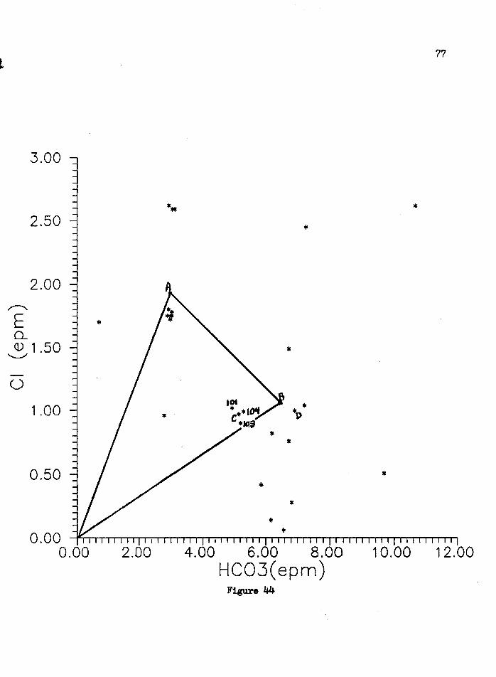
Mixing Diagrams Figures 24-44

Table 12 Key to Mixing Diagrams

Letters A, B, C, and D, represent the Average Ionic Concentrations From

Table 7 for Their Respective Water Source

A= Scioto River

B= Glac1al-Outwash Aquifer

C= Collector Wells

D= Carbonate Aquifer

56

........-....

E 0... Q)

........__,.

0 u

10.00

8.00

6.00

4.00

2.00

0.00 0.00

5?

•

• ... ..

•

2.00 4.00 6.00 8.00 10.00 12.00 HC03(epm)

Figure 24

58

/

5.00

* 4.00

.. o **

• • * ~

E 3.oo * Q_

Q) '-..._./

CJ)

2 2.00

1.00

0 . 0 0 -f'T-:.....-r"T".,........,....~....-.-r"'T""'T""'T""i......,...-r"T-r-r-T'"~l'""T""T"'T"T""T"'T""T'"T"""T""'1r"'T""T"'T"-r-r-T'""........,....,.....-r"T""T'""'T""T"""r-T""'T""T""'1

0.00 2.00 4.00 6.00 8.00 10.00 12.00 HC03(epm)

Figure 25

/

2.50

2.00

...--..... E 1.50 Q_ Q)

"-..,./

0 z 1.00

*

0.50

* •

...

*

* *

*

*

59

+

.o *

*

0. 00 -"'4-.............-.-~ ............... .,...........,. ............... .,...........,........,....,..~.......,....,.."r"'"T'-.-r_.......,...~ ............................................. .,...........,....,....,

0.00 2.00 4.00 6.00 8.00 10.00 12.C HC03 (epm)

Figure 26

60

0.25

0.20

.,,,-........_

E 0.15 Q_ * Q) ~

• ~

0.10

101 * • *

C-• ldl

•O

0.05

*

0. 00 -f'llP-,..........,......,.....................-r-P___...."T""T""T"",_..........,.""'P'""'T'""P"~,_..........,...,..........................,..........,.......,....,.......,..........._,~...,....,......~

0.00 2.00 4.00 6.00 8.00 1 0.00 12.00 HC03(epm)

Figure 27

5.00

4.00

~ 0 (f) 2.00

1.00

0.00 0.00

*

* •

2.00

61

*

* * * •o *

* •

• *

4.00 6.00 8.00 10.00 12.00 HC03(e~m)

Figure 28

5.00

4.00

,............_,

E 3.oo 0.. (}) .....__,,,

-tj-

0 (/) 2.00

1.00

0.00 0.00

*

*

I

2.00

62

*

* * * * D * * •

* * *

10]

* *

*

*

I

4.00 6.00 8.00 10.00 Ca (epm)

Figure 29

5.00

4.00

,.....--....

E 3.oo Q_ Q) ........__,

'tj-

0 (f) 2.00

1.00

0.00 0.00

I

'i.00

* ** ...

2.00 Mg

*

3.00 (epm)

Figure 30

*

*

63

* *

* *O *

*

4.00 5.00

64

5.00

•

• 4.00 • • • 0 • • •

* •• *

~

E 3.oo 0.. Q)

..........._,, '23 • ~ f 0 (/) 2.00

*

* *

1.00

0 . 0 0 -1'-T-...-.-.-..,.....,.....,..,.....,.....,-.--.-.....-r-r-,....,....,_.....,......,..-:-T-"T"_,....,......,.~........-r"'T.....,......,....,.....,.....,-.--r-l ............... ,....,....,_"T"""T"'"T'"

0.00 0.50 1 .00 1 .50 2.00 2.50 Na (epm)

Figure 31

5.00

4.00

,---.._

E 3.oo 0... Q)

.....__,,,,,

~ 0 (/) 2.00

1.00

0.00 0.00

•

•

'f

*

0.05

•

• • * • * •D

* • •

103 • * c. *

101

*

0.10 0.15 0.20 0.25

K~~m)

I

0.25

0.20

,,.,,....-....

E o.1s Q_ Q)

........._,,,

~

0.10

0.05

0.00 0.00

*

2.00

66

...

* * ...

•

*

I

4.00 6.00 8.00 10.00 Ca (epm)

Figure 33

0.25

0.20

,...,--......

E 0.1 s I o_

Q) ........__,,,,

~

0.10

0.05

6?

**

*

* *

*

0.00 ~~.,.-,-,r-r-.-~ ............ .....--.-...-.-............ .....--.-.,.-,-,.........,...,....,...-r-.,..-,r-r-r-.-.-T""T"""l~..,....,...T"""T"""r...,......."T-i

0.00 ~ .00 2.00 3.00 4.00 5.00 Mg (epm)

Figure J4

0.25

0.20

,--........

E 0.15 o_ Q) .......__,,

~

0.10

0.05

0.00 0.00

*

0.50

68

** •

•

*

* ••D

• • • • •• JO'/

1 .00 1 .50 2.00 2.50 Na ( epm)

Figure 3.S

2.50

2.00

,....--...., E 1.50 Q_ Q)

"'-./

0 z 1.00

0.50

0.00 0.00

/

*

*

2.00

...

* •

101 *

...

*

.o

• *

•

4.00 6.00 Ca (epm)

Figure J6

69

*

•

8.00 10.0:

2.50

2.00

~

E 1.so o_ Q) ...__.,,,

0

z 1.00

0.50

0.00 0.00

./

·./

•

I 1.00

• *

2.00 Mg

•

• *

3.00 (epm)

Figure 37

•

*

•

70

•

•

*

* /0

•

•

4.00 5.00

5.00

4.00

.......--...._

E 3.oo 0.. Q) ....__.,,,

OJ 2

2.00

1.00

*

•

D • • * * • * *

71

*

0.00 -llL-r-.-.-.......................... ~1-.-.-...-.-.~-.-.-r-T"""!"-r-r-~-.-.-............ _...... ............ .......,..............,....,...,...,._,,.....,~

0.00 2.00 4.00 6.00 8.00 10.00 Ca (epm)

Figure J8

3.00

2.50

2.00 ........--.....

E ~ o_

(}) ....._,, 1 .50

u

1.00

0.50

?2

*

*

*

*

* • *

* 0.00 ~~,...,_...-,.-.-,..---.-r-T'""T""T"""ir-r-T"~,....,_,.~,...,......-r-T'".,....,....r-r-r"~T"T"""'l-r-T'""T""T"""i......,......~

0.00 2.00 4.00 6.00 8.00 10.00 Ca (epm)

Figure 39

73

3.00

* 2.50 •

2.00 ..........-..

~~ • Q)

.............. 1 .50 *

u

1.00 •D

• *

0.50 * • *

• 0. 00 ~......---.-....-...-..""r'"T"""'r---...........-............... __.....~ .............. ,_.....,... ............... _......~...._.. .............. ............,....,.._..._...,

0.00 1.00 2.00 3.00 4.00 5.00 Mg (epm)

Figure 40

3.00

2.50

2.00 ,,..,--....

E ~ .fr

-..._...-1 .50

u

1.00

0.50

0.00 0.00 0.50

?4

*

*

1.00 1.50 2.00 2.50 Na (eprn)

Figure 41

75

3.00

* * ; 2.50

*

2.00 .......--...

E o_ * Q)

-..__..., 1 .50

u

1.00 *

0.50 *

*

0. 00 -.,._...._ .............. ~......---.-.---..........--.-.............. _........ .............. .,......_ ............. _........._.........,,........._ .............. _____..... 0.00 0.05 0.10 0.15 0.20 0.25

K (epm) .... Figure 42

5.00

4.00

,...---...

E 3.oo Q_ Q)

........._,,,

~ 0 (f) 2.00

1.00

0.00 0.00

* *

•

• *

0.50

?6

•

... ... ** * * D

""" **

* •

103 * *

f.101

* •

1 .00 1 .50 2.00 2.50 3.00 Cl (eprr.)

Figure 4J

3.00

* 2.50

2.00

*

0

1.00 • * ~

• *

0.50 *

* •

0.00 --~.........-T'"'I ............................. ,..........,...~~~............,...,....,...._.,....,........., ............... ...-........ .............. ............,..~~ 0.00 2.00 4.00 6.00 8.00 10.00 12.00

HC03(epm) Figure 44