Embed Size (px)
Citation preview
HAL Id: hal-01307750https://hal.inria.fr/hal-01307750v4
Submitted on 11 Jan 2018
HAL is a multi-disciplinary open accessarchive for the deposit and dissemination of sci-entific research documents, whether they are pub-lished or not. The documents may come fromteaching and research institutions in France orabroad, or from public or private research centers.
L’archive ouverte pluridisciplinaire HAL, estdestinée au dépôt et à la diffusion de documentsscientifiques de niveau recherche, publiés ou non,émanant des établissements d’enseignement et derecherche français ou étrangers, des laboratoirespublics ou privés.
Copyright
Arbogast: Higher order automatic differentiation forspecial functions with Modular C
Isabelle Charpentier, Jens Gustedt
To cite this version:Isabelle Charpentier, Jens Gustedt. Arbogast: Higher order automatic differentiation for specialfunctions with Modular C. Optimization Methods and Software, Taylor & Francis, 2018, 33 (4-6),pp.963-987. �10.1080/10556788.2018.1428603�. �hal-01307750v4�
ISS
N02
49-6
399
ISR
NIN
RIA
/RR
--89
07--
FR+E
NG
RESEARCHREPORTN° 8907Apr. 2016
Project-Team Camus
ArbogastHigher order AD forspecial functions withModular CIsabelle Charpentier and Jens Gustedt

RESEARCH CENTRENANCY – GRAND EST
615 rue du Jardin BotaniqueCS2010154603 Villers-lès-Nancy Cedex
Arbogast
Higher order AD for special functions withModular C∗
Isabelle Charpentier† and Jens Gustedt‡
Project-Team Camus
Research Report n° 8907 — version 4 — initial version Apr. 2016 —revised version Jan. 2018 — 21 pages
Abstract: This high-level toolbox for the calculus with Taylor polynomials is named afterL.F.A. Arbogast (1759–1803), a French mathematician from Strasbourg (Alsace), for his pioneeringwork in derivation calculus.Arbogast is based on a well-defined extension of the C programming language, Modular C, andplaces itself between tools that proceed by operator overloading on one side and by rewriting, onthe other. The approach is best described as contextualization of C code because it permits theprogrammer to place his code in different contexts – usual math or AD – to reinterpret it as ausual C function or as a differential operator. Because of the type generic features of modern C,all specializations can be delegated to the compiler. The HOAD with arbogast is exemplified onfamilies of functions of mathematical physics and on models for complex dielectric functions usedin optics.
Key-words: automatic differentiation, differential operators, modular programming, C, contex-tualization, functions of mathematical physics
∗ Accepted for publication in Optimization Methods and Software† ICube, CNRS and Universite de Strasbourg, France‡ Inria, France
Arbogast
DA d’ordre eleve avec Modular C pour des fonctionsspeciales
Resume :Cette boite a outil pour le calcul avec les polynomes de Taylor est nomme aprs L.F.A. Arbo-
gast (1759–1803), mathematicien francais de Strasbourg, Alsace, pour son travail pionnier sur lecalcul des derivations.
Arbogast est base sur une extension du langage de programmation C, Modular C, et seplace entre des outil travaillant avec la surcharge d’operateurs et ceux faisant de la reecriture.L’approche est mieux decrit en tant que contextualisation de code C, car il permet au program-meur de placer son code en contextes differents – habituellement mathematique ou DA – pour lereinterpreter comme fonction C usuelle ou comme operateur differentiel. Due au caracteristiquesde genericite de types du C moderne, toute specialisation peut etre deleguee au compilateur.La differentiation automatique a haut degree avec arbogast est exemplifiee avec des familles defonction de physique mathematiques et avec des modeles de fonctions dielectriques complexesutilisees en optique.
Mots-cles : differentiation automatique, operateurs differentielles, programmation modulaire,C, contextualisation, fonctions speciales
Arbogast: Higher order AD for special functions with Modular C 3
1 Introduction and Overview
From the time that L.F.A. Arbogast [1, 2, 3] wrote the “Calcul des derivations”, the higher-order derivationof compound mathematical functions has been extensively studied [4, 5]. Nowadays, see [6] for instance, thehigher-order automatic differentiation (HOAD) of computer codes representing complex compound mathemati-cal functions mainly relies on operator overloading as a technique for attaching well-known recurrence formulasto arithmetic operations and intrinsic functions of programming languages such as C++, FORTRAN 90 orMatlab. A list of packages that allow for the differentiation of C++ codes is provided on the AutoDiff site.Beyond that, the differentiation of linear solvers or linear transformations, fixed-point methods [7], nonlinearsolvers [8, 9] and special functions of mathematical physics [10] requires a careful study to be accurate andefficient. Although general developments were proposed and automated for most of these issues, they are notsystematically included in the existing AD tools.
Since decades, C is one of the most widely used programming languages [11] and is used successfully for largesoftware projects that are ubiquitous in modern computing devices of all scales. To the best of our knowledge,the AutoDiff site only references possible usages of C++ operator overloading libraries on C codes that do notcontain C-specific features, and the source transformation tool ADIC [12, 13] for differentiating C codes1 upto the second order. In this paper, we discuss the implementation and validation of a modular HOAD librarycalled arbogast dedicated to modern ISO C that includes second order operators for the HOAD of classicalfunctions of mathematical physics [14, 15] and has the potential to integrate other of the specialized algorithms,eventually.
C is undergoing a continued process of standardization and improvement and, over the years, has addedfeatures that are important in the context of this study: complex numbers, variable length arrays (VLA), longdouble, the restrict keyword, type generic mathematical functions (all in C99), programmable type generic
interfaces (_Generic), choosable alignment and Unicode support (in C11), see [16]. Contrary to common belief,C is not a subset of C++. Features such as VLA, restrict and _Generic that make C interesting for numericalcalculus do not translate to C++. Moreover, its static type system, fixed at compile time, and its ability tomanage pointer aliasing make C particularly interesting for performance critical code. These are properties thatare not met by C++, where dynamic types, indirections and opaque overloading of operators can be a severeimpediment for compiler optimization. Unfortunately, these advantages of C are met with some shortcomings.Prominent among these is the lack of two closely related features, modularity and reusability, that are highlydesirable in the context of automatic differentiation.
To propose a HOAD tool for C, we consider an extension to the C standard called Modular C [17] thatenables us to cope with the identified lack of modularity and reusability. Modular C consists in the addition toC of a handful of directives and a naming scheme transforming traditional translation units (TU) into modules.The goal of this paper is to prove that this extension allows us to implement efficient, modular, extensible andmaintainable code for automatic differentiation, while preserving the properties of C that we appreciate fornumerical code. Named arbogast, the resulting modular AD tool we present provides a high-level toolbox forunivariate calculus with Taylor polynomials. For a method to extend this approach to multivariate tensors theinterested reader is refered to [18, 10]. It places itself between tools that proceed by operator overloading on oneside, and by rewriting on the other. The approach is better described as contextualization or reinterpretationof code. The HOAD with arbogast is exemplified on models for complex dielectric functions, one of themcomprising a function of mathematical physics.
This paper is organized as follows. The aims and abilities of Modular C are introduced in Section 2 andillustrated on an implementation of a generalized Heron’s method to compute νth roots. The new AD library,arbogast, is described in Section 3. Subsequently we demonstrate the usefulness of our HOAD tool by designinga differential operator (DO) devoted to the solution for the general 2nd order ODE satisfied by most of thefunctions of mathematical physics in Section 4, then an application to optics in Section 5. All these codeexamples are accompanied by benchmarks that prove the efficiency of our approach. Section 6 presents someconclusions and outlooks.
2 Modular C
For many programmers, software projects and commercial enterprises C has advantages – relative simplicity,faithfulness to modern architectures, backward and forward compatibility – that largely outweigh its short-comings. Among these shortcomings is a lack of modularity and reusability due to the fact that C misses toencapsulate different translation units. All symbols of all used interfaces are shared and may clash when theyare linked together into an executable. A common practice to cope with that difficulty is the use of namingconventions. Usually software units (modules) are attributed a name prefix that is used for all data typesand functions that constitute the programmable interface (API). Such naming conventions (and more generally
1ADIC only handles the historic C89 version, often referred to as “ANSI C”.
RR n° 8907
Arbogast: Higher order AD for special functions with Modular C 4
coding styles) are often perceived as a burden. They require a lot of self-discipline and experience, and C ismissing features that would support or ease their application.
2.1 Modularity for AD and Taylor polynomials
Because of its requirement for code efficiency, AD can profit substantially from code written in C. Unfortunatelythough, an AD tool has a strong need for genericity and modularity since it has to be able to deal with numericalcodes that possibly involve 6 different floating point types (float, double, long double and their complexvariants). Then, 3 binary operations on Taylor polynomials have to be implemented covering the case whereboth operands are polynomials, but also for the case that one of them is a scalar. In a complete support libraryfor AD we would have to produce similar code for the combination of all 6 floating types and 3 combinations ofoperands, so 18 replicas in total. This growing code complexity gets even worse when we want to special-casecertain types of operations, for instance to take advantage of polynomials with different degrees.
Other programming languages than plain C are able to cope better with such a combinatorial explosion ofcases. In particular, C++ offers implicit type conversion and template programming that can (and have been)used to implement operators generically. A typical C++ implementation would first implement Taylor-to-Tayloroperators as template. This would give rise to only 6 instantiations. When such an operator is called by usercode, the arguments, Taylor or scalar, would be converted to a common “super” type T, then the appropriateoperator for T would be called.
Whereas this quickly provides a solution for the problem, such code is generally not as efficient as it couldbe. A lot of intermediate values (Taylor polynomials) will be produced during execution, all arithmetic willalways be performed in the wider and more expensive version, and if objects are passed by reference (or pointer)aliasing restrictions can undermine optimization. Moreover, when using templates, C++ typically would deferthe compilation of a particular instantiation of a template to the compilation that uses it, leading to prohibitivecompilation times of user code. Although partial solutions exist to circumvent these problems, their generaleffect may result in a degradation of the modularity properties that had motivated the choice for C++ in thefirst place.
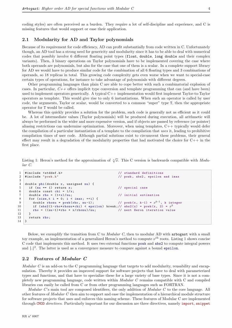
Listing 1: Heron’s method for the approximation of ν√x. This C version is backwards compatible with Modu-
lar C.
1 #include <stddef.h> // standard definitions
2 #include "powk.h" // powk , abs2 , epsilon and imax
34 double phi(double x, unsigned nu) {
5 if (nu == 1) return x; // special case
6 double const chi = 1/x;
7 double rho = (1+x)/nu; // initial estimation
8 for (size_t i = 0; i < imax; ++i) {
9 double rhonu = powk(rho , nu -1); // powk(x, k-1) = xk−1, k integer
10 if (abs2(1-rho*rhonu*chi) < epsilon) break;// abs2(x) = powk(x, 2) = x2
11 rho = ((nu -1)*rho + x/rhonu)/nu; // next Heron iteration value
12 }
13 return rho;
14 }
Below, we exemplify the transition from C to Modular C, then to modular AD with arbogast with a smalltoy example, an implementation of a generalized Heron’s method to compute νth roots. Listing 1 shows conciseC code that implements this method. It uses two external functions powk and abs2 to compute integral powersand ∥.∥2. The latter is used as a convergence measure to compare against a bound epsilon.
2.2 Features of Modular C
Modular C is an add-on to the C programming language that targets to add modularity, reusability and encap-sulation. Thereby it provides an improved support for software projects that have to deal with parameterizedtypes and functions, and that have to specialize these for a large variety of base types. Since it is not a com-pletely new programming language, code written within Modular C remains compatible with C and compiledlibraries can easily be called from C or from other programming languages such as FORTRAN.
Modular C ’s main tool are composed identifiers, the only addition of Modular C to the core language. Allother features of Modular C then aim to support and ease the implementation of a hierarchical module structurefor software projects that uses and enforces this naming scheme. These features of Modular C are implementedthrough CMOD directives. Particularly important for our discussion are three directives, namely import, snippet
RR n° 8907
Arbogast: Higher order AD for special functions with Modular C 5
and foreach. We will discuss and exemplify them below in more detail. Another feature that is particularlyinteresting for AD is contextualization. It provides a replacement for operator overloading as we will see whenwe discuss arbogast in Section 3.
Additional features of Modular C are a dynamic module initialization scheme, a structured approach to theC library, a migration path for existing software projects and, last but not least, complete Unicode integration.
2.2.1 Composed identifiers
Composed identifiers are segmented by a user-chosable character2. The basic rules for interpretation of such anidentifier are straightforward, the segmented prefix of an identifier corresponds to the module (translation unit)where that identifier can be found. For instance, C::io::printf refers to the printf function in the module C::ioand arbogast::trd refers to the Taylor polynomial type trd (Taylor real double) in the arbogast module. Aslong as segmented identifiers are used in this long form, they can be used freely anywhere they make sense. Allnecessary information is encoded in that name and no #include or import directive is needed.
2.2.2 Import directive
Modules can import other modules as long as the import relation remains acyclic. As we already have mentionedabove, such an import can be implicit if a long segmented identifier is used, or it can be explicit by means of animport directive. Other than traditional #include, import ensures complete encapsulation between modules.
The advantage of using the directive over implicit import is the abbreviation scheme. It allows to refer to allidentifiers of another module with a short prefix, and it also allows to seamlessly replace an imported moduleby another one with equivalent interface.
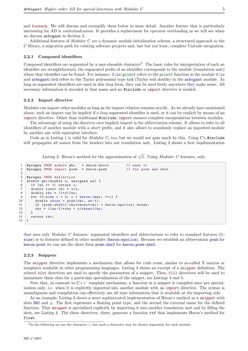
Code as in Listing 1 is valid for Modular C, too, but we would not gain much by this. Using C’s #include
still propagates all names from the headers into our translation unit. Listing 2 shows a first implementation
Listing 2: Heron’s method for the approximation of ν√x. Using Modular C features, only.
1 #pragma CMOD module phi = heron ::droot // name it
2 #pragma CMOD import powk = heron ::powk // for powk and abs2
34 #pragma CMOD definition
5 double phi(double x, unsigned nu) {
6 if (nu == 1) return x;
7 double const chi = 1/x;
8 double rho = (1+x)/nu;
9 for (C ::size i = 0; i < heron ::imax; ++i) {
10 double rhonu = powk(rho , nu -1);
11 if (powk ::abs2(1-rho*rhonu*chi) < heron ::epsilon) break;
12 rho = ((nu -1)*rho + x/rhonu)/nu;
13 }
14 return rho;
15 }
that uses only Modular C features: segmented identifiers and abbreviations to refer to standard features (C::size) or to features defined in other modules (heron::epsilon). Because we establish an abbreviation powk forheron::powk we can use the short form powk::abs2 for heron::powk::abs2.
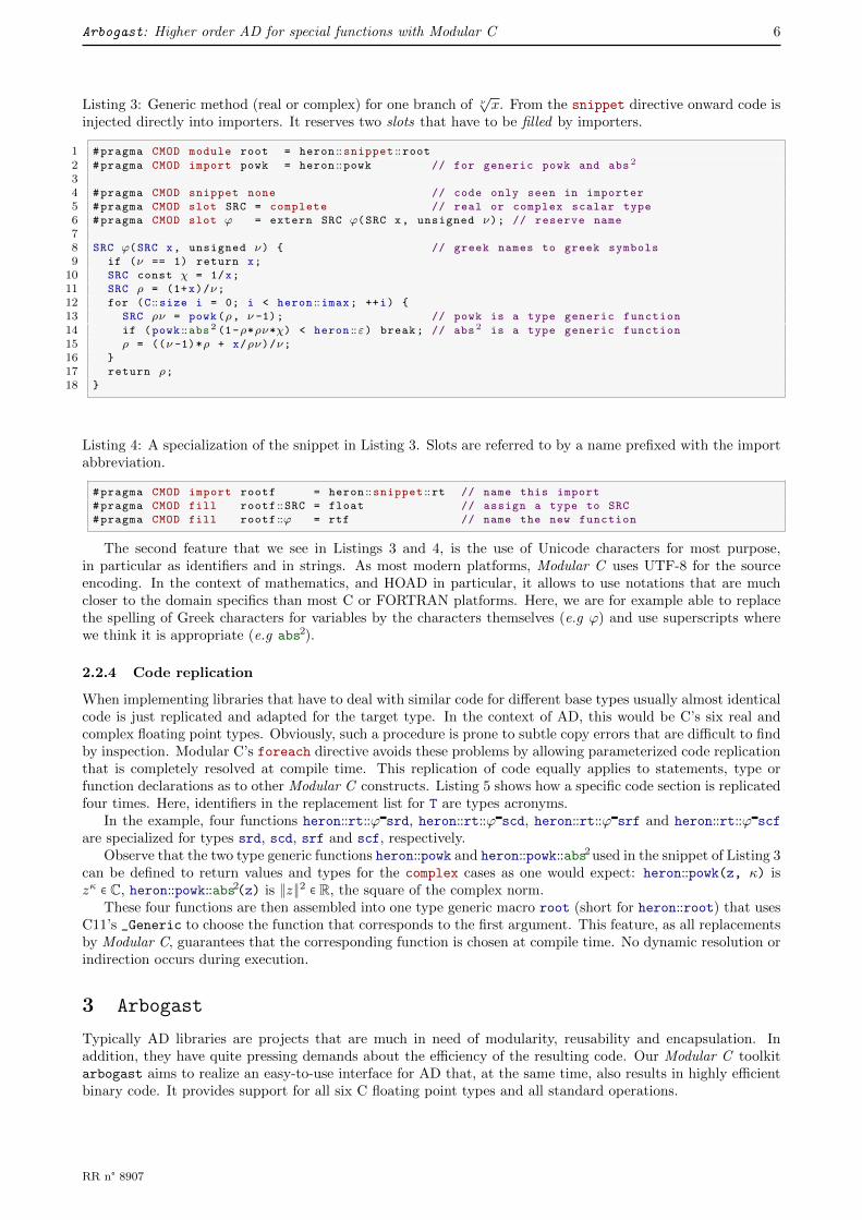
2.2.3 Snippets
The snippet directive implements a mechanism that allows for code reuse, similar to so-called X macros ortemplates available in other programming languages. Listing 3 shows an excerpt of a snippet definition. Therelated slot directives are used to specify the parameters of a snippet. Then, fill directives will be used toinstantiate these slots for a particular specialization of the snippet, see Listings 4 and 5.
Note that, in contrast to C++’ template mechanism, a function in a snippet is compiled once per special-ization only, i.e. when it is explicitly imported into another module with an import directive. The syntax isunambiguous and compilation can effectively use all type information that is available at the importing side.
As an example, Listing 3 shows a more sophisticated implementation of Heron’s method as a snippet withslots SRC and ϕ. The first represents a floating point type, and the second the external name for the definedfunction. That snippet is specialized explicitly by importing it into another translation unit and by filling theslots, see Listing 4. The three directives, there, generate a function rtf that implements Heron’s method forfloat.
2In the following we use the character ::, but such a character may be chosen separately for each module.
RR n° 8907
Arbogast: Higher order AD for special functions with Modular C 6
Listing 3: Generic method (real or complex) for one branch of ν√x. From the snippet directive onward code is
injected directly into importers. It reserves two slots that have to be filled by importers.
1 #pragma CMOD module root = heron ::snippet ::root2 #pragma CMOD import powk = heron ::powk // for generic powk and abs 2
34 #pragma CMOD snippet none // code only seen in importer
5 #pragma CMOD slot SRC = complete // real or complex scalar type
6 #pragma CMOD slot ϕ = extern SRC ϕ(SRC x, unsigned ν); // reserve name
78 SRC ϕ(SRC x, unsigned ν) { // greek names to greek symbols
9 if (ν == 1) return x;
10 SRC const χ = 1/x;
11 SRC ρ = (1+x)/ν;12 for (C ::size i = 0; i < heron ::imax; ++i) {
13 SRC ρν = powk(ρ, ν -1); // powk is a type generic function
14 if (powk ::abs 2 (1-ρ*ρν*χ) < heron ::ε) break; // abs 2 is a type generic function
15 ρ = ((ν -1)*ρ + x/ρν)/ν;16 }
17 return ρ;18 }
Listing 4: A specialization of the snippet in Listing 3. Slots are referred to by a name prefixed with the importabbreviation.
#pragma CMOD import rootf = heron ::snippet ::rt // name this import
#pragma CMOD fill rootf ::SRC = float // assign a type to SRC
#pragma CMOD fill rootf ::ϕ = rtf // name the new function
The second feature that we see in Listings 3 and 4, is the use of Unicode characters for most purpose,in particular as identifiers and in strings. As most modern platforms, Modular C uses UTF-8 for the sourceencoding. In the context of mathematics, and HOAD in particular, it allows to use notations that are muchcloser to the domain specifics than most C or FORTRAN platforms. Here, we are for example able to replacethe spelling of Greek characters for variables by the characters themselves (e.g ϕ) and use superscripts wherewe think it is appropriate (e.g abs2).
2.2.4 Code replication
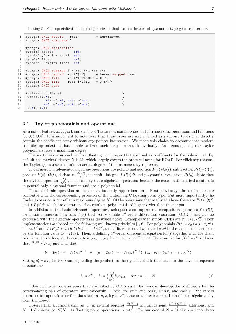
When implementing libraries that have to deal with similar code for different base types usually almost identicalcode is just replicated and adapted for the target type. In the context of AD, this would be C’s six real andcomplex floating point types. Obviously, such a procedure is prone to subtle copy errors that are difficult to findby inspection. Modular C’s foreach directive avoids these problems by allowing parameterized code replicationthat is completely resolved at compile time. This replication of code equally applies to statements, type orfunction declarations as to other Modular C constructs. Listing 5 shows how a specific code section is replicatedfour times. Here, identifiers in the replacement list for T are types acronyms.
In the example, four functions heron::rt::ϕ srd, heron::rt::ϕ scd, heron::rt::ϕ srf and heron::rt::ϕ scf
are specialized for types srd, scd, srf and scf, respectively.Observe that the two type generic functions heron::powk and heron::powk::abs2used in the snippet of Listing 3
can be defined to return values and types for the complex cases as one would expect: heron::powk(z, κ) iszκ ∈ C, heron::powk::abs2(z) is ∥z∥2 ∈ R, the square of the complex norm.
These four functions are then assembled into one type generic macro root (short for heron::root) that usesC11’s _Generic to choose the function that corresponds to the first argument. This feature, as all replacementsby Modular C, guarantees that the corresponding function is chosen at compile time. No dynamic resolution orindirection occurs during execution.
3 Arbogast
Typically AD libraries are projects that are much in need of modularity, reusability and encapsulation. Inaddition, they have quite pressing demands about the efficiency of the resulting code. Our Modular C toolkitarbogast aims to realize an easy-to-use interface for AD that, at the same time, also results in highly efficientbinary code. It provides support for all six C floating point types and all standard operations.
RR n° 8907
Arbogast: Higher order AD for special functions with Modular C 7
Listing 5: Four specializations of the generic method for one branch of ν√x and a type generic interface.
1 #pragma CMOD module root = heron ::root2 #pragma CMOD composer
34 #pragma CMOD declaration
5 typedef double srd;
6 typedef _Complex double scd;
7 typedef float srf;
8 typedef _Complex float scf;
910 #pragma CMOD foreach T = srd scd srf scf
11 #pragma CMOD import root ${T} = heron ::snippet ::root12 #pragma CMOD fill root ${T} ::SRC = ${T}13 #pragma CMOD fill root ${T} ::ϕ = ϕ ${T}14 #pragma CMOD done
1516 #define root(X, N) \
17 _Generic ((X), \
18 srd: ϕ srd , scd: ϕ scd , \
19 srf: ϕ srf , scf: ϕ scf) \
20 ((X), (N))
3.1 Taylor polynomials and operations
As a major feature, arbogast implements 6 Taylor polynomial types and corresponding operations and functions[6, 303–308]. It is important to note here that these types are implemented as structure types that directlycontain the coefficient array without any pointer indirection. We made this choice to accommodate moderncompiler optimization that is able to track such array elements individually. As a consequence, our Taylorpolynomials have a maximum degree.
The six types correspond to C’s 6 floating point types that are used as coefficients for the polynomial. Bydefault the maximal degree N is 31, which largely covers the practical needs for HOAD. For efficiency reasons,the Taylor types also maintain an actual degree of the instance they represent.
The principal implemented algebraic operations are polynomial addition P (t)+Q(t), subtraction P (t)−Q(t),
product P (t) ⋅Q(t), derivative dP (t)dt
, indefinite integral ∫ P (t)dt and polynomial evaluation P (t0). Note that
the division operator, P (t)Q(t)
, is not among these algebraic operations because the exact mathematical solution is
in general only a rational function and not a polynomial.These algebraic operation are not exact but only approximations. First, obviously, the coefficients are
computed with the corresponding precision of the underlying C floating point type. But more importantly, theTaylor expansion is cut off at a maximum degree N . Of the operations that are listed above these are P (t) ⋅Q(t)and ∫ P (t)dt which are operations that result in polynomials of higher order than their input.
In addition to the basic arithmetic operators, arbogast also implements composition operators f ○ P (t)for major numerical functions f(x) that verify simple 1st-order differential equations (ODE), that can beexpressed with the algebraic operations as dissussed above. Examples with simple ODEs are ex, 1/x,
√x. Their
implementations are based on the following well-known principles [1, 6]. For polynomials P (t) = a0+a1t+a2t2+
⋯+aN tN and f ○P (t) ≈ b0+b1t+b2t
2+⋯+bN tN , the additive constant b0, called seed in the sequel, is determined
by the function value b0 = f(a0). Then, a defining 1st-order differential equation for f together with the chainrule is used to subsequently compute b1, b2, . . . , bN by equating coefficients. For example for f(x) = ex we know
that df(x)dx
= f(x) and thus that
b1 + 2b2t +⋯ +NbN tN−1
≈ (a1 + 2a2t +⋯ +NaN tN−1
) ⋅ (b0 + b1t + b2t2+⋯ + bN t
N)
Setting a′k = kak for k > 0 and expanding the product on the right hand side then leads to the solvable sequenceof equations:
b0 = ea0 , bj =
1j
j−1
∑k=0
bka′
j−k for j = 1, . . .N (1)
Other functions come in pairs that are linked by ODEs such that we can develop the coefficients for thecorresponding pair of operators simultaneously. These are sinx and cosx, sinhx, and coshx. Yet othersoperators for operations or functions such as y/x, logx, xν , tanx or tanhx can then be combined algebraicallyfrom the above.
Observe that a formula such as (1) in general requires N(N−1)2
multiplications, (N−1)(N−2)2
additions, andN − 1 divisions, so N(N − 1) floating point operations in total. For our case of N = 31 this corresponds to
RR n° 8907
Arbogast: Higher order AD for special functions with Modular C 8
an overhead of 930 floating point operations per Taylor operator. As a consequence we can expect a “Taylor”program F′ that is derived from a conventional program F by replacing floating point variables by Taylorpolynomials to be several orders of magnitude slower than F.
But fortunately this overhead for AD is only additive, that is, any closed expression that uses n of thealgebraic or numerical floating point operations from above should only encounter n times this overhead whentransformed into an operator for Taylor polynomials. Therefore we will use the complexity of the most commonlyused operators, namely the division operator, as a baseline for performance discussions, below.
3.2 Contextualization
The snippet in Listing 3 is type generic and could almost serve as a base to be used with arbogast for AD,just by “filling” with one of arbogast’s Taylor polynomial types instead of a floating point type. As C doesnot provide the possibility of overloading arithmetic operations, the type generic programming described aboveis only possible through functional notation.
One way to differentiate the numerical code in Listing 3 would be to manually rewrite the snippet such thatall necessary arithmetic operators are replaced by function calls. For instance, we could replace each divisionthat potentially could be a polynomial division by a call to arbogast::div.
Listing 6: A generic method for an approximation of one branch of ν√x or ν
√x0 + x1t + x2t2 +⋯. The specialized
context for arithmetic with the parameter type RC is coded inside (: :) brackets.
1 #pragma CMOD module heron ::snippet ::rt2 #pragma CMOD import powk = heron ::powk // scalars or Taylor types
34 #pragma CMOD snippet none
5 #pragma CMOD context AD = (: :) // overload some expressions
6 #pragma CMOD slot RC = complete // scalar or Taylor type
7 #pragma CMOD slot ϕ = extern RC ϕ(RC x, unsigned ν);89 RC ϕ(RC x, unsigned ν) {
10 if (ν == 1) return x;
11 RC const χ = (:1/x:); // may be polynomial division
12 RC ρ = (:(1+x)/ν :);13 for (C ::size i = 0; i < heron ::imax; ++i) { // conventional operations
14 RC ρν = powk(ρ, ν -1); // no context needed
15 if ((:powk ::abs 2 (1-ρ*ρν*χ) < heron ::ε:)) break; // compare to a real value
16 ρ = (:((ν -1)*ρ + x/ρν)/ν :);17 }
18 return ρ;19 }
Modular C offers a easier way to do this: the context directive. This allows to choose opening and closing“parenthesis” that mark a special context in an expression and replace all occurrences of arithmetic operatorsby proper function calls. In Listing 6 we define a context, locally named AD, that starts with a (: and endswith a :). Then we mark all places that might involve arithmetic with Taylor polynomials by these characters.For instance, the division in Line 11 could be either scalar arithmetic if x is a scalar, or polynomial division ifx is a Taylor polynomial. Note that using the AD context for the convergence criterion in Line 15 is mainly fordemonstrative purpose. The computation here only uses the 0th Taylor coefficients.
Modular C allows to define several contexts inside the same module. The strings for opening or closingparenthesis can be chosen quite freely. Listing 7 shows a specialization of the snippet with arbogast’s six
Listing 7: Six specializations of the generic method for one branch of ν√x0 + x1t + x2t2 +⋯.
1 #pragma CMOD module heron ::inst ::rt ::AD2 #pragma CMOD import arbogast ::taylor3 #pragma CMOD composer
45 #pragma CMOD foreach TRC = trf tcf trd tcd trl tcl
6 #pragma CMOD import rt ${TRC} = heron ::snippet ::rt7 #pragma CMOD fill rt ${TRC} ::AD = arbogast ::context8 #pragma CMOD fill rt ${TRC} ::RC = ${TRC}9 #pragma CMOD fill rt ${TRC} ::ϕ = ϕ ${TRC}
10 #pragma CMOD done
RR n° 8907
Arbogast: Higher order AD for special functions with Modular C 9
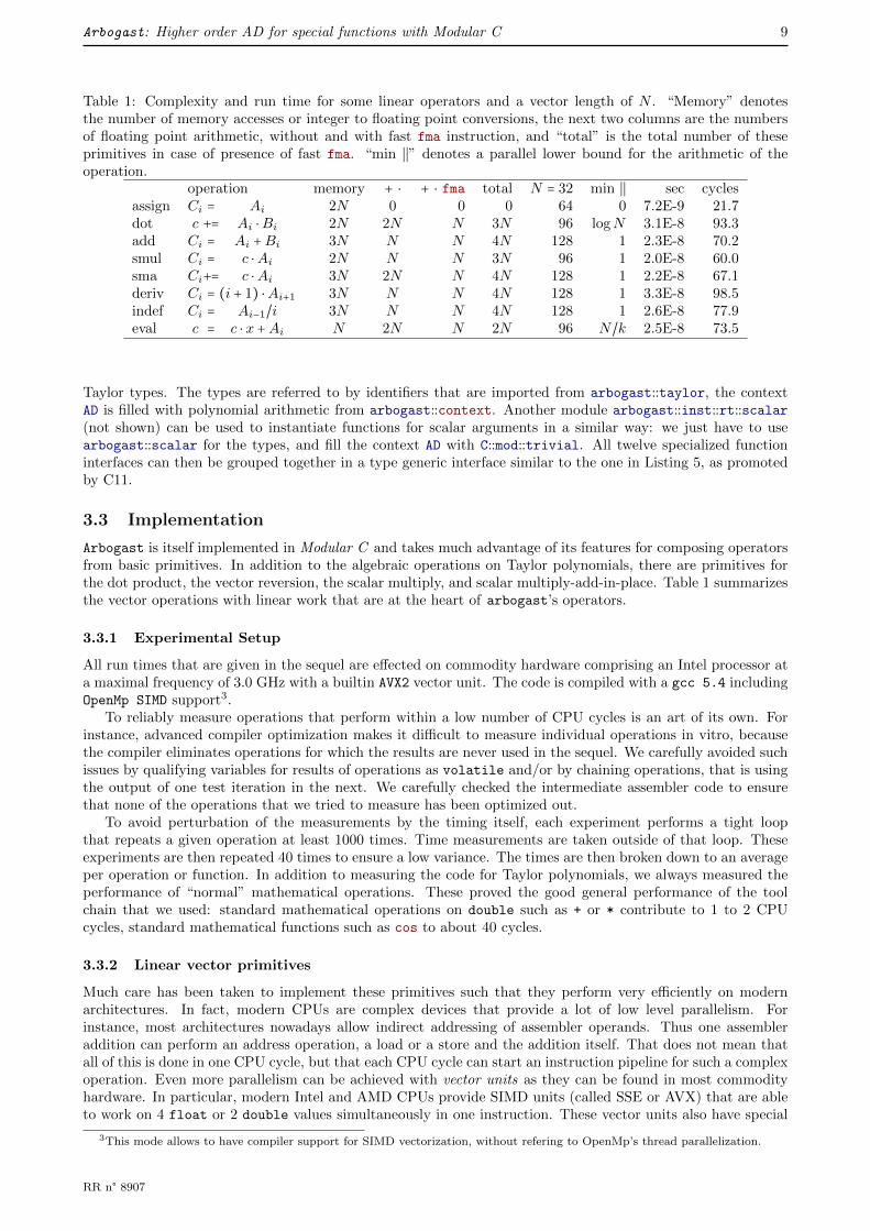
Table 1: Complexity and run time for some linear operators and a vector length of N . “Memory” denotesthe number of memory accesses or integer to floating point conversions, the next two columns are the numbersof floating point arithmetic, without and with fast fma instruction, and “total” is the total number of theseprimitives in case of presence of fast fma. “min ∣∣” denotes a parallel lower bound for the arithmetic of theoperation.
operation memory + ⋅ + ⋅ fma total N = 32 min ∣∣ sec cyclesassign Ci = Ai 2N 0 0 0 64 0 7.2E-9 21.7dot c += Ai ⋅Bi 2N 2N N 3N 96 logN 3.1E-8 93.3add Ci = Ai +Bi 3N N N 4N 128 1 2.3E-8 70.2smul Ci = c ⋅Ai 2N N N 3N 96 1 2.0E-8 60.0sma Ci+= c ⋅Ai 3N 2N N 4N 128 1 2.2E-8 67.1deriv Ci = (i + 1) ⋅Ai+1 3N N N 4N 128 1 3.3E-8 98.5indef Ci = Ai−1/i 3N N N 4N 128 1 2.6E-8 77.9eval c = c ⋅ x +Ai N 2N N 2N 96 N/k 2.5E-8 73.5
Taylor types. The types are referred to by identifiers that are imported from arbogast::taylor, the contextAD is filled with polynomial arithmetic from arbogast::context. Another module arbogast::inst::rt::scalar(not shown) can be used to instantiate functions for scalar arguments in a similar way: we just have to usearbogast::scalar for the types, and fill the context AD with C::mod::trivial. All twelve specialized functioninterfaces can then be grouped together in a type generic interface similar to the one in Listing 5, as promotedby C11.
3.3 Implementation
Arbogast is itself implemented in Modular C and takes much advantage of its features for composing operatorsfrom basic primitives. In addition to the algebraic operations on Taylor polynomials, there are primitives forthe dot product, the vector reversion, the scalar multiply, and scalar multiply-add-in-place. Table 1 summarizesthe vector operations with linear work that are at the heart of arbogast’s operators.
3.3.1 Experimental Setup
All run times that are given in the sequel are effected on commodity hardware comprising an Intel processor ata maximal frequency of 3.0 GHz with a builtin AVX2 vector unit. The code is compiled with a gcc 5.4 includingOpenMp SIMD support3.
To reliably measure operations that perform within a low number of CPU cycles is an art of its own. Forinstance, advanced compiler optimization makes it difficult to measure individual operations in vitro, becausethe compiler eliminates operations for which the results are never used in the sequel. We carefully avoided suchissues by qualifying variables for results of operations as volatile and/or by chaining operations, that is usingthe output of one test iteration in the next. We carefully checked the intermediate assembler code to ensurethat none of the operations that we tried to measure has been optimized out.
To avoid perturbation of the measurements by the timing itself, each experiment performs a tight loopthat repeats a given operation at least 1000 times. Time measurements are taken outside of that loop. Theseexperiments are then repeated 40 times to ensure a low variance. The times are then broken down to an averageper operation or function. In addition to measuring the code for Taylor polynomials, we always measured theperformance of “normal” mathematical operations. These proved the good general performance of the toolchain that we used: standard mathematical operations on double such as + or * contribute to 1 to 2 CPUcycles, standard mathematical functions such as cos to about 40 cycles.
3.3.2 Linear vector primitives
Much care has been taken to implement these primitives such that they perform very efficiently on modernarchitectures. In fact, modern CPUs are complex devices that provide a lot of low level parallelism. Forinstance, most architectures nowadays allow indirect addressing of assembler operands. Thus one assembleraddition can perform an address operation, a load or a store and the addition itself. That does not mean thatall of this is done in one CPU cycle, but that each CPU cycle can start an instruction pipeline for such a complexoperation. Even more parallelism can be achieved with vector units as they can be found in most commodityhardware. In particular, modern Intel and AMD CPUs provide SIMD units (called SSE or AVX) that are ableto work on 4 float or 2 double values simultaneously in one instruction. These vector units also have special
3This mode allows to have compiler support for SIMD vectorization, without refering to OpenMp’s thread parallelization.
RR n° 8907
Arbogast: Higher order AD for special functions with Modular C 10
fast fused multiply-add (fma) instructions that in the case of float can perform 4 such operations, that is 8FLOPs, in a single CPU instruction4.
Table 1 shows the vector operations that are at the basis of Taylor polynomial operations as they areimplemented by arbogast and their average execution times on a recent commodity platform. They havevarying efficiency and in particular we see that the dot product operation is much slower than a scalar-multiply-add-in-place operation “sma”. This is due to the fact that the former has a logarithmic parallel overhead forthe computation of the final sum and that the latter can profit from a fast fma operation. Below we will see howthis performance difference is used to speedup arbogast substantially compared to a direct implementation offormulas such as (1).
For the evaluation of polynomials at a given point x we use Estrin’s [19] variation of Horner’s method [20].This method allows for vector parallelization and proves to be very efficient. Its performance is comparableto polynomial addition. In particular, for a given special function the time for an evaluation of the Taylorpolynomial can be faster than the evaluation of the function itself.
3.3.3 Product formulas
The first non-trivial Taylor operator to implement is the product P (t) ⋅Q(t) of two polynomials. The genericformula for such a product is similar to formula (1), but with the difference that all the terms are independent:
ck = ∑i+j=k
ai ⋅ bj =k
∑i=0
ai ⋅ bk−i (2)
As already discussed, a direct implementation of such a formula for N = 31 needs to perform at least 930floating point operations. But we cannot expect all the vectors and partial results to fit in CPU registers duringthe whole computation, so values generally must be stored to and reloaded from memory. Thereby a directimplementation of these formulas without vector unit and without indirect addressing will normally accountfrom 2 to 3 times the number of CPU cycles. So typically, a HOAD operator will use several thousand CPUcycles more than the scalar operation that it replaces.
A challenge to implement such formulas efficiently when using a vector unit stems from the fact that thevector of the second term in the sum (b in (2)) is accessed in reverse order. Such downward accesses have aperformance hit on vector units. We can avoid these by reversing the vector b first, then using a sequence ofdot products to perform the summation. With the performance measures that we have seen above this wouldamount to lower bound of a cycle count for float of
Tdiv + Trevert +N
2Tdot = 70 + 20 + 16 ⋅ 65 = 1130.
We can do much better when implementing (1) differently. In fact, as soon as a particular coefficient biis computed, its scalar multiple with the vector a′ can be computed and added to the partial sums of thecoefficients bi+1, . . . , bN . When using scalar-multiply-add-in-place operations (5th line in Table 1) this leads toa lower bound on the instruction count of about 70 + 16 ⋅ 46 = 806.
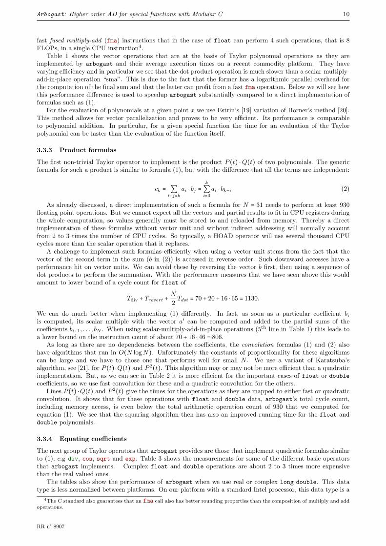
As long as there are no dependencies between the coefficients, the convolution formulas (1) and (2) alsohave algorithms that run in O(N logN). Unfortunately the constants of proportionality for these algorithmscan be large and we have to chose one that performs well for small N . We use a variant of Karatsuba’salgorithm, see [21], for P (t) ⋅Q(t) and P 2(t). This algorithm may or may not be more efficient than a quadraticimplementation. But, as we can see in Table 2 it is more efficient for the important cases of float or doublecoefficients, so we use fast convolution for these and a quadratic convolution for the others.
Lines P (t) ⋅Q(t) and P 2(t) give the times for the operations as they are mapped to either fast or quadraticconvolution. It shows that for these operations with float and double data, arbogast’s total cycle count,including memory access, is even below the total arithmetic operation count of 930 that we computed forequation (1). We see that the squaring algorithm then has also an improved running time for the float anddouble polynomials.
3.3.4 Equating coefficients
The next group of Taylor operators that arbogast provides are those that implement quadratic formulas similarto (1), e.g div, cos, sqrt and exp. Table 3 shows the measurements for some of the different basic operatorsthat arbogast implements. Complex float and double operations are about 2 to 3 times more expensivethan the real valued ones.
The tables also show the performance of arbogast when we use real or complex long double. This datatype is less normalized between platforms. On our platform with a standard Intel processor, this data type is a
4The C standard also guarantees that an fma call also has better rounding properties than the composition of multiply and addoperations.
RR n° 8907
Arbogast: Higher order AD for special functions with Modular C 11
Table 2: Taylor product operators, measured in CPU cycles, for N = 31.real real real complex complex complex
float double long double float double long double
quadradic conv. 809.0 897.7 2585.2 2312.1 2818.3 11204.5fast conv. 607.5 753.8 5053.2 2695.0 3996.9 17968.8P (t) ⋅Q(t) 634.8 792.4 2605.6 2325.0 2900.5 11356.2P 2(t) 516.1 627.8 2557.6 2316.2 2852.5 11245.5
Table 3: Quadratic Taylor operations of standard mathematical functions or operations, measured in CPUcycles, for N = 31. The functions of the first group are implemented directly, those of the second are implementedas compositions of other operators.
real real real complex complex complexfloat double long double float double long double
div 974.2 922.8 2718.8 2416.8 3235.8 11711.9cos 1176.0 1424.6 9516.4 4062.2 5065.0 20469.7sqrt 1556.4 1300.2 1281.8 2064.4 2029.6 6748.3exp 1260.3 1498.1 2816.3 2606.1 3393.4 11047.8log 1345.0 1389.4 3248.3 2919.4 3885.0 13367.2pow 2641.0 2748.2 6765.9 5666.4 7015.7 23713.6
Table 4: Quadratic Taylor operations of standard mathematical functions or operations, measured in div
operations. The functions of the first group are implemented directly, those of the second are implemented ascompositions of other operators.
real real real complex complex complexfloat double long double float double long double
div 1.0 1.0 1.0 1.0 1.0 1.0cos 1.2 1.5 3.5 1.7 1.6 1.7sqrt 1.6 1.4 0.5 0.9 0.6 0.6exp 1.3 1.6 1.0 1.1 1.0 0.9log 1.4 1.5 1.2 1.2 1.2 1.1pow 2.7 3.0 2.6 2.4 2.5 2.1
RR n° 8907
Arbogast: Higher order AD for special functions with Modular C 12
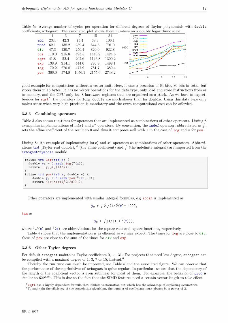
Table 5: Average number of cycles per operation for different degrees of Taylor polynomials with double
coefficients, arbogast. The associated plot shows these numbers on a doubly logarithmic scale.1 3 7 15 31
add 23.4 42.3 75.4 68.3 106.1prod 62.1 138.2 259.4 544.3 791.0div 47.3 120.7 256.4 820.0 922.8cos 119.0 215.8 493.5 1448.2 1424.6sqrt 41.8 52.4 202.6 1146.8 1300.2exp 138.9 214.1 444.0 795.9 1498.1log 172.2 270.8 477.9 781.7 1389.4pow 366.0 574.8 1056.1 2155.6 2748.2
good example for computations without a vector unit. Here, it uses a precision of 64 bits, 80 bits in total, butstores them in 16 bytes. It has no vector operations for the data type, only load and store instructions from orto memory, and the CPU only has 8 hardware registers that are organized as a stack. As we have to expect,besides for sqrt5, the operators for long double are much slower than for double. Using this data type onlymakes sense when very high precision is mandatory and the extra computational cost can be afforded.
3.3.5 Combining operators
Table 3 also shows run-times for operators that are implemented as combinations of other operators. Listing 8exemplifies implementations of ln(x) and xν operators. By convention, the indef operator, abbreviated as ∫ ,sets the affine coefficient of the result to 0 and thus it composes well with + in the case of log and * for pow.
Listing 8: An example of implementing ln(x) and xν operators as combinations of other operators. Abbrevi-ations trd (Taylor real double), 0 (the affine coefficient) and ∫ (the indefinite integral) are imported from thearbogast symbols module.
inline trd log(trd x) {
double y0 = C ::math ::log(0 (x));
return (:y0 + ∫ (1/x):);}
inline trd pow(trd x, double ν) {
double y0 = C ::math ::pow(0 (x), ν);return (:y0 *exp(∫ (ν/x)):);
}
Other operators are implemented with similar integral formulas, e.g acosh is implemented as
y0 + ∫ (2√(1/(2(x)- 1))),
tan as
y0 + ∫ (1/(1 + 2(x))),
where 2√(x) and 2(x) are abbreviations for the square root and square functions, respectively.Table 4 shows that the implementation is as efficient as we may expect. The times for log are close to div,
those of pow are close to the sum of the times for div and exp.
3.3.6 Other Taylor degrees
Per default arbogast maintains Taylor coefficients 0, . . . ,31. For projects that need less degree, arbogast canbe compiled with a maximal degree of 1, 3, 7 or 15, instead.6
Thereby the run time can much be improved, see Table 5 and the associated figure. We can observe thatthe performance of these primitives of arbogast is quite regular. In particular, we see that the dependency ofthe length of the coefficient vector is even sublinear for most of them. For example, the behavior of prod issimilar to 62N3/4. This is due to the fact that the SIMD features need a certain vector length to take effect.
5sqrt has a highly dependent formula that inhibits vectorization but which has the advantage of exploiting symmetries.6To maintain the efficiency of the convolution algorithm, the number of coefficients must always be a power of 2.
RR n° 8907
Arbogast: Higher order AD for special functions with Modular C 13
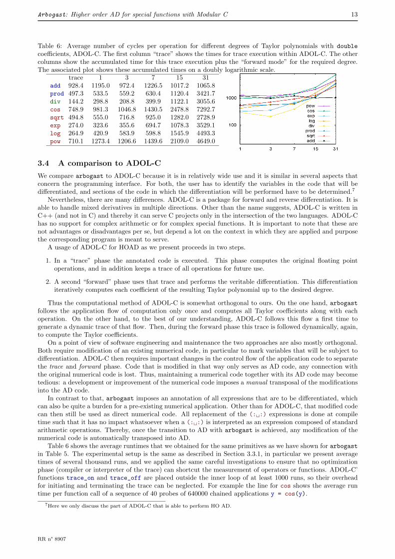
Table 6: Average number of cycles per operation for different degrees of Taylor polynomials with double
coefficients, ADOL-C. The first column “trace” shows the times for trace execution within ADOL-C. The othercolumns show the accumulated time for this trace execution plus the “forward mode” for the required degree.The associated plot shows these accumulated times on a doubly logarithmic scale.
trace 1 3 7 15 31add 928.4 1195.0 972.4 1226.5 1017.2 1065.8prod 497.3 533.5 559.2 630.4 1120.4 3421.7div 144.2 298.8 208.8 399.9 1122.1 3055.6cos 748.9 981.3 1046.8 1430.5 2478.8 7292.7sqrt 494.8 555.0 716.8 925.0 1282.0 2728.9exp 274.0 323.6 355.6 694.7 1078.3 3529.1log 264.9 420.9 583.9 598.8 1545.9 4493.3pow 710.1 1273.4 1206.6 1439.6 2109.0 4649.0
3.4 A comparison to ADOL-C
We compare arbogast to ADOL-C because it is in relatively wide use and it is similar in several aspects thatconcern the programming interface. For both, the user has to identify the variables in the code that will bedifferentiated, and sections of the code in which the differentiation will be performed have to be determined.7
Nevertheless, there are many differences. ADOL-C is a package for forward and reverse differentiation. It isable to handle mixed derivatives in multiple directions. Other than the name suggests, ADOL-C is written inC++ (and not in C) and thereby it can serve C projects only in the intersection of the two languages. ADOL-Chas no support for complex arithmetic or for complex special functions. It is important to note that these arenot advantages or disadvantages per se, but depend a lot on the context in which they are applied and purposethe corresponding program is meant to serve.
A usage of ADOL-C for HOAD as we present proceeds in two steps.
1. In a “trace” phase the annotated code is executed. This phase computes the original floating pointoperations, and in addition keeps a trace of all operations for future use.
2. A second “forward” phase uses that trace and performs the veritable differentiation. This differentiationiteratively computes each coefficient of the resulting Taylor polynomial up to the desired degree.
Thus the computational method of ADOL-C is somewhat orthogonal to ours. On the one hand, arbogastfollows the application flow of computation only once and computes all Taylor coefficients along with eachoperation. On the other hand, to the best of our understanding, ADOL-C follows this flow a first time togenerate a dynamic trace of that flow. Then, during the forward phase this trace is followed dynamically, again,to compute the Taylor coefficients.
On a point of view of software engineering and maintenance the two approaches are also mostly orthogonal.Both require modification of an existing numerical code, in particular to mark variables that will be subject todifferentiation. ADOL-C then requires important changes in the control flow of the application code to separatethe trace and forward phase. Code that is modified in that way only serves as AD code, any connection withthe original numerical code is lost. Thus, maintaining a numerical code together with its AD code may becometedious: a development or improvement of the numerical code imposes a manual transposal of the modificationsinto the AD code.
In contrast to that, arbogast imposes an annotation of all expressions that are to be differentiated, whichcan also be quite a burden for a pre-existing numerical application. Other than for ADOL-C, that modified codecan then still be used as direct numerical code. All replacement of the (: :) expressions is done at compiletime such that it has no impact whatsoever when a (: :) is interpreted as an expression composed of standardarithmetic operations. Thereby, once the transition to AD with arbogast is achieved, any modification of thenumerical code is automatically transposed into AD.
Table 6 shows the average runtimes that we obtained for the same primitives as we have shown for arbogastin Table 5. The experimental setup is the same as described in Section 3.3.1, in particular we present averagetimes of several thousand runs, and we applied the same careful investigations to ensure that no optimizationphase (compiler or interpreter of the trace) can shortcut the measurement of operators or functions. ADOL-C’functions trace_on and trace_off are placed outside the inner loop of at least 1000 runs, so their overheadfor initiating and terminating the trace can be neglected. For example the line for cos shows the average runtime per function call of a sequence of 40 probes of 640000 chained applications y = cos(y).
7Here we only discuss the part of ADOL-C that is able to perform HO AD.
RR n° 8907
Arbogast: Higher order AD for special functions with Modular C 14
Table 7: Parametric functions used as seeds, second order equations and validation formulas for some orthogonalpolynomials.
Seed [14, 22.8] Second order ODE [15, 18.8.1] Validation [15, 10.6.1]Name ϕν aν bν gν αν βν γν Aν Bν Gν
Ultraspherical C(λ)ν 1 − z2 −νz ν + 2λ − 1 1 − z2 −(2λ + 1)z ν(ν + 2λ) 1 2(ν+λ)
ν+1z ν+2λ−1
ν+1Chebyshev Tν 1 − z2 −νz ν 1 − z2 −z ν2 1 (2 − δν,0)z 1Chebyshev Uν 1 − z2 −νz ν + 1 1 − z2 −3z ν(ν + 2) 1 2z 1Legendre Pν 1 − z2 −νz ν 1 − z2 −2z ν(ν + 1) 1 2ν+1
ν+1z ν
ν+1
Gen. Laguerre L(λ)ν z ν −(ν + λ) z λ + 1 − z ν 1 − z+2ν+λ+1
ν+1ν+λν+1
Hermite Hν 1 0 2ν 1 −2z 2ν 1 2z 2νHermite Heν 1 0 ν 1 −z ν 1 z ν
The first column shows the average time that these operations need for the trace, before any differentiationis effected. The other columns then show the overall average time for the whole operation in question, suchthat the numbers can directly be compared with those for arbogast.
The resulting times for ADOL-C have a very high variance and have to be taken with a lot of reserve. Athorough micro-benchmarking and review would have probably been convenient, but the C++ code of ADOL-C is so complex that we found it beyond our possibilities to investigate plausible causes for such an erraticbehavior. Consequently, we have no explanation to offer why the addition operation in ADOL-C has such ahigh overhead for the trace phase, and we don’t know if the running times for exp and log are significantlydistinct.
Nevertheless after taking into account these uncertainties, we see that the trace phase (not the initiationor termination of the phase) has an important impact on the runtime of each of the operations and that itclearly forms a bottleneck of the computation8. We attribute this to the fact that tracing tracks the sequenceof operations dynamically, resulting in a lot of dynamic allocations, indirections, cache misses, pipeline stallsand far jumps through the binary executable.
In our opinion, the lack of performance of ADOL-C is due to an unfortunate combination of two strategiesthat makes the code optimization by the compiler very difficult. First, the trace code uses a lot of indirectionsthat are inherent to the operator overloading technique. They are quite challenging to any optimizing compiler,because of their side effects and their aliasing and because they interrupt the “natural” control flow of theapplication. But second, during the forward phase the sequence of operations is not directly visible to thecompiler, but interpreted dynamically at run time from the trace. Thus, optimization opportunities that couldprofit from compile-time knowledge about a whole sequence of operations may be missed.
For the considered use case of HOAD, arbogast’s runtime is significantly better than ADOL-C in most ofthe cases. ADOL-C operates and performs similar to interpreted languages. Therefore a completely compiledapproach in C as provided by arbogast may outperform it to the extent that we see in our measurements.
4 Operators for the HOAD of special functions
Special functions and their derivatives play a crucial role in research fields of physics and mathematical analysis.As reported in [14, 15], many of these functions are solutions of the general second order ordinary differentialequation (ODE)
α(z)ϕ(2)(z) + β(z)ϕ(1)
(z) + γ(z)ϕ(z) = 0, (3)
where the input z is either a real or a complex variable, and functions α(z), β(z), γ(z) determine the math-ematical function ϕ(z). In other words, seeds ϕ(0)(z) = ϕ(z) and ϕ(1)(z) = dϕ
dz(z), and functions α(z), β(z),
γ(z) may be used to evaluate the second order derivative ϕ(2)(z) = d2ϕdz2
(z), then higher-order derivatives. Forthe sake of generality in the presentation, we also adopt the same general seed formula and notation for theorthogonal polynomials, Tab. 7, the Bessel functions, Tab. 8, and the hypergeometric functions, Tab. 9. Notethat other formulas are available and can be used to deal with special cases, see for instance [22].
In the past, considerable research efforts have been directed at implementing special functions in numericallibraries (some of them are proposed in the GNU Scientific Library), without, however, having developed genuineactivities within the context of AD. This paper builds on [10, 23, 24] to propose formulas and operators that allowfor the automatic generation of the higher-order automatic differentiation library arbogast for mathematicalfunctions satisfying (3), then for its validation.
8ADOL-C has a special mode for first order differentiation that does not need the trace phase.
RR n° 8907
Arbogast: Higher order AD for special functions with Modular C 15
Table 8: Parametric functions used as seeds, second order equations and validation formulas for representativeBessel functions.
Seed Second order ODE ValidationBessel ϕν aν bν gν Ref. αν βν γν Ref. Aν Bν Gν Ref.Bessel Jν 1 -ν
z1 (10.6.1) z2 z (z2 − ν2) (10.2.1) 1 2ν
z1 (10.6)
Modified Iν 1 -νz
1 (10.29.1) z2 z −(z2 + ν2) (10.25.1) 1 − 2νz
-1 (10.29)Spherical jν 1 -ν+1
z1 (10.51.1) z2 2z z2 − ν(ν + 1) (10.47.1) 1 2ν+1
z1 (10.51)
Table 9: Parametric functions used as second order equations and validation formulas for some hypergeometricfunctions.
Second order ODE ValidationHyp. Geo. ϕ α(z) β(z) γ(z) Ref. A(ν) B(z) G(z) Ref.Kummer M z µ − z −ν (13.2.1) ν 2ν − µ + z µ − ν (13.3.1)Whitaker U z µ − z −ν (13.2.1) ν(ν − µ + 1) µ − 2ν − z 1 (13.3.7)Gauss 2F1 z − z2 ξ − (ν + µ + 1)z −νµ (15.10.1) ν(z − 1) ξ − 2ν − (µ − ν)z ξ − ν (15.5.11)
4.1 Second order ODE
The key difference between [14] and AD is in the definition of z. AD considers z as a function z(t) depending onsome variable t and implements it as a Taylor polynomial, the coefficients of which are classically denoted by zk,
k = 0, ...,N , and satisfy zk =1k!∂kz∂tk
. The second order differentiation of the compound function v(t) = ϕ○z(t) [25]is here carried out by applying the chain rule to (3). This yields the general formulation (4),
v(0) = ϕ(0)(z(0)), v(1) = ϕ(1)(z(0))z(1),
v(2) =−γv(0)(z(1))
3− βv(1)(z(1))
2+ αv(1)z(2)
αz(1), for z(1) ≠ 0.
(4)
This can be overloaded for the higher-order differentiation of v(t) = ϕ ○ z(t) [25]. Equating coefficients leads toan implementation of v(t) which is of quadratic worst-case complexity [24], O(N2), where N is the maximaldegree of a Taylor polynomial. The special case of z(1) = 0 is discussed in [25].
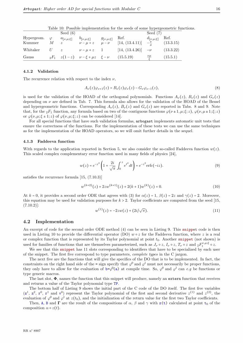
4.1.1 Seeds
Equation (4) requires the evaluation of the function ϕ and its derivative at the point of development, thatcan then be used as seeds for equating coefficients. Whereas an implementation of ϕ is usually available, animplementation of its derivative might not. But many parameterized families of functions provide recurrencerelations that relate functions and their derivatives. With arbogast we are able to use these recurrence relationsto actually compute the derivative where necessary.
The families of orthogonal polynomials, Bessel functions, and hypergeometric functions are constituted intogroups of parameterized functions with specific names and very similar relationships. To avoid any confusionwith the differentiation order k, we use the same leading index ν to denote either the degree in an orthogonalpolynomial sequence, or the “main” parameter in the other functions. The interested reader is referred to[14, 15] for parameter ranges.
Under this convention, these three families of functions meet the general first order differential relation,
aν(z)ϕ(1)ν (z) = bν(z)ϕν(z) + gν(z)ϕν−1(z), (5)
that defines the seed ϕ(1)ν by means of functions aν(z), bν(z) and gν(z).
For instance, the first derivative of the hypergeometric function ϕ(ν,µ; ξ; z), the parameters of which arehere denoted by ν, µ, and possibly ξ, satisfies
a[ν,µ;ξ](z)ϕ(1)
(ν,µ; ξ; z) = b[ν,µ;ξ](z)ϕ(ν,µ; ξ; z) + g[ν,µ;ξ](z)ϕ(ν − 1, µ; ξ; z). (6)
Functions a[ν,µ;ξ](z), b[ν,µ;ξ](z) and g[ν,µ;ξ](z) related to the confluent hypergeometric functions M(ν,µ; z) andU(ν,µ; z), and the hypergeometric function 2F1(ν,µ; ξ; z) are reported in Tab. 10. Additionally, these familiesof functions have recurrence relations for all two (respectively three) parameters. This leads to formulas thatonly refer to ϕ(ν + 1, µ + 1; ξ + 1; z) multiplied by a scalar d[ν,µ;ξ]
ϕ(1)(ν,µ; ξ; z) = d[ν,µ;ξ]ϕ(ν + 1, µ + 1; ξ + 1; z). (7)
Since it also avoids a polynomial division by the a[ν,µ;ξ] term, arbogast uses Equation (7) to implement ϕ(1)
for the hypergeometric functions.
RR n° 8907
Arbogast: Higher order AD for special functions with Modular C 16
Table 10: Possible implementation for the seeds of some hypergeometric functions.Seed (6) Seed (7)
Hypergeom. ϕ a[ν,µ;ξ] b[ν,µ;ξ] g[ν,µ;ξ] Ref. d[ν,µ;ξ] Ref.Kummer M z ν − µ + z µ − ν [14, (13.4.11)] − ν
µ(13.3.15)
Whitaker U z ν − µ + z 1 [14, (13.4.26)] −ν (13.3.22)
Gauss 2F1 z(1 − z) ν − ξ + µz ξ − ν (15.5.19) νµξ
(15.5.1)
4.1.2 Validation
The recurrence relation with respect to the index ν,
Aν(z)ϕν+1(z) = Bν(z)ϕν(z) −Gνϕν−1(z), (8)
is used for the validation of the HOAD of the orthogonal polynomials. Functions Aν(z), Bν(z) and Gν(z)depending on ν are defined in Tab. 7. This formula also allows for the validation of the HOAD of the Besseland hypergeometric functions. Corresponding Aν(z), Bν(z) and Gν(z) are reported in Tabs. 8 and 9. Notethat, for the 2F1 function, any formula based on two of the contiguous functions ϕ(ν ±1, µ; ξ; z), ϕ(ν,µ±1; ξ; z)or ϕ(ν,µ; ξ ± 1; z) of ϕ(ν,µ; ξ; z) can be considered [14].
For all special functions that have such validation formulas, arbogast implements automatic unit tests thatensure the correctness of the functions. For the implementation of these tests we can use the same techniquesas for the implementation of the HOAD operators, so we will omit further details in the sequel.
4.1.3 Faddeeva function
With regards to the application reported in Section 5, we also consider the so-called Faddeeva function w(z).This scaled complex complementary error function used in many fields of physics [24],
w(z) = e−z2
(1 +2i√π∫
z
0et
2
dt) = e−z2
erfc(−iz). (9)
satisfies the recurrence formula [15, (7.10.3)]
w(k+2)(z) + 2zw(k+1)
(z) + 2(k + 1)w(k)(z) = 0. (10)
At k = 0, it provides a second order ODE that agrees with (3) for α(z) = 1, β(z) = 2z and γ(z) = 2. Moreover,this equation may be used for validation purposes for k > 2. Taylor coefficients are computed from the seed [15,(7.10.2)]:
w(1)(z) = −2zw(z) + (2i/
√π). (11)
4.2 Implementation
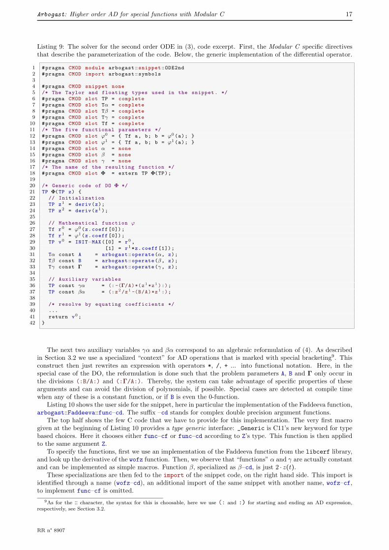
An excerpt of code for the second order ODE method (4) can be seen in Listing 9. This snippet code is thenused in Listing 10 to provide the differential operator (DO) w ○ z for the Faddeeva function, where z is a realor complex function that is represented by its Taylor polynomial at point t0. Another snippet (not shown) is
used for families of functions that are themselves parameterized, such as Jν ○ z, Iν ○ z, Tν ○ z and 2Fν,µ;ξ1 ○ z.
We see that this snippet has 11 slots corresponding to identifiers that have to be specialized by each userof the snippet. The first five correspond to type parameters, complete types in the C jargon.
The next five are the functions that will give the specifics of the DO that is to be implemented. In fact, theconstraints on the right hand side of the = sign specify that ϕ0 and ϕ1 must not necessarily be proper functions,they only have to allow for the evaluation of b=ϕ0(a) at compile time. So, ϕ0 and ϕ1 can e.g be functions ortype generic macros.
The last slot, Φ, names the function that this snippet will produce, namely an extern function that receivesand returns a value of the Taylor polynomial type TP.
The bottom half of Listing 9 shows the initial part of the C code of the DO itself. The first five variables(z1, z2, r0, r1 and v0) represent the Taylor polynomial of the first and second derivative z(1) and z(2), theevaluation of ϕ0 and ϕ1 at z(t0), and the initialization of the return value for the first two Taylor coefficients.
Then, A, B and Γ are the result of the compositions of α, β and γ with z(t) calculated at point t0 of thecomposition α ○ z(t).
RR n° 8907
Arbogast: Higher order AD for special functions with Modular C 17
Listing 9: The solver for the second order ODE in (3), code excerpt. First, the Modular C specific directivesthat describe the parameterization of the code. Below, the generic implementation of the differential operator.
1 #pragma CMOD module arbogast ::snippet ::ODE2nd2 #pragma CMOD import arbogast ::symbols34 #pragma CMOD snippet none
5 /* The Taylor and floating types used in the snippet. */
6 #pragma CMOD slot TP = complete
7 #pragma CMOD slot Tα = complete
8 #pragma CMOD slot Tβ = complete
9 #pragma CMOD slot Tγ = complete
10 #pragma CMOD slot Tf = complete
11 /* The five functional parameters */
12 #pragma CMOD slot ϕ0 = { Tf a, b; b = ϕ0 (a); }
13 #pragma CMOD slot ϕ1 = { Tf a, b; b = ϕ1 (a); }
14 #pragma CMOD slot α = none
15 #pragma CMOD slot β = none
16 #pragma CMOD slot γ = none
17 /* The name of the resulting function */
18 #pragma CMOD slot Φ = extern TP Φ(TP);
1920 /* Generic code of DO Φ */
21 TP Φ(TP z) {
22 // Initialization
23 TP z1 = deriv(z);
24 TP z2 = deriv(z1 );
2526 // Mathematical function ϕ27 Tf r0 = ϕ0 (z.coeff [0]);
28 Tf r1 = ϕ1 (z.coeff [0]);
29 TP v0 = INIT–MAX ([0] = r0 ,
30 [1] = r1 *z.coeff [1]);
31 Tα const A = arbogast ::operate(α, z);
32 Tβ const B = arbogast ::operate(β, z);
33 Tγ const Γ = arbogast ::operate(γ, z);
3435 // Auxiliary variables
36 TP const γα = (: -(Γ/A)*(z1 *z1 ):);
37 TP const βα = (:z2 /z1 -(B/A)*z1 :);
3839 /* resolve by equating coefficients */
40 ...
41 return v0 ;
42 }
The next two auxiliary variables γα and βα correspond to an algebraic reformulation of (4). As describedin Section 3.2 we use a specialized “context” for AD operations that is marked with special bracketing9. Thisconstruct then just rewrites an expression with operators *, /, + ... into functional notation. Here, in thespecial case of the DO, the reformulation is done such that the problem parameters A, B and Γ only occur inthe divisions (:B/A:) and (:Γ/A:). Thereby, the system can take advantage of specific properties of thesearguments and can avoid the division of polynomials, if possible. Special cases are detected at compile timewhen any of these is a constant function, or if B is even the 0-function.
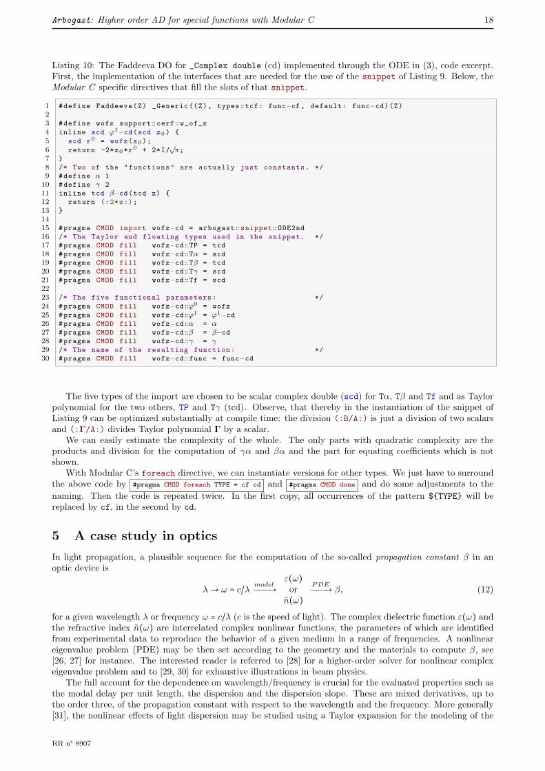
Listing 10 shows the user side for the snippet, here in particular the implementation of the Faddeeva function,arbogast::Faddeeva::func–cd. The suffix –cd stands for complex double precision argument functions.
The top half shows the few C code that we have to provide for this implementation. The very first macrogiven at the beginning of Listing 10 provides a type generic interface: _Generic is C11’s new keyword for typebased choices. Here it chooses either func–cf or func–cd according to Z’s type. This function is then appliedto the same argument Z.
To specify the functions, first we use an implementation of the Faddeeva function from the libcerf library,and look up the derivative of the wofz function. Then, we observe that “functions” α and γ are actually constantand can be implemented as simple macros. Function β, specialized as β–cd, is just 2 ⋅ z(t).
These specializations are then fed to the import of the snippet code, on the right hand side. This import isidentified through a name (wofz–cd), an additional import of the same snippet with another name, wofz–cf,to implement func–cf is omitted.
9As for the :: character, the syntax for this is choosable, here we use (: and :) for starting and ending an AD expression,respectively, see Section 3.2.
RR n° 8907
Arbogast: Higher order AD for special functions with Modular C 18
Listing 10: The Faddeeva DO for _Complex double (cd) implemented through the ODE in (3), code excerpt.First, the implementation of the interfaces that are needed for the use of the snippet of Listing 9. Below, theModular C specific directives that fill the slots of that snippet.
1 #define Faddeeva(Z) _Generic ((Z), types ::tcf: func–cf, default: func–cd)(Z)23 #define wofz support ::cerf ::w_of_z4 inline scd ϕ1–cd(scd z0 ) {
5 scd r0 = wofz(z0 );
6 return -2*z0 *r0 + 2*I/
√π;
7 }
8 /* Two of the "functions" are actually just constants. */
9 #define α 1
10 #define γ 2
11 inline tcd β–cd(tcd z) {
12 return (:2*z:);
13 }
1415 #pragma CMOD import wofz–cd = arbogast ::snippet ::ODE2nd16 /* The Taylor and floating types used in the snippet. */
17 #pragma CMOD fill wofz–cd ::TP = tcd
18 #pragma CMOD fill wofz–cd ::Tα = scd
19 #pragma CMOD fill wofz–cd ::Tβ = tcd
20 #pragma CMOD fill wofz–cd ::Tγ = scd
21 #pragma CMOD fill wofz–cd ::Tf = scd
2223 /* The five functional parameters: */
24 #pragma CMOD fill wofz–cd ::ϕ0 = wofz
25 #pragma CMOD fill wofz–cd ::ϕ1 = ϕ1–cd26 #pragma CMOD fill wofz–cd ::α = α27 #pragma CMOD fill wofz–cd ::β = β–cd28 #pragma CMOD fill wofz–cd ::γ = γ29 /* The name of the resulting function: */
30 #pragma CMOD fill wofz–cd ::func = func–cd
The five types of the import are chosen to be scalar complex double (scd) for Tα, Tβ and Tf and as Taylorpolynomial for the two others, TP and Tγ (tcd). Observe, that thereby in the instantiation of the snippet ofListing 9 can be optimized substantially at compile time: the division (:B/A:) is just a division of two scalarsand (:Γ/A:) divides Taylor polynomial Γ by a scalar.
We can easily estimate the complexity of the whole. The only parts with quadratic complexity are theproducts and division for the computation of γα and βα and the part for equating coefficients which is notshown.
With Modular C’s foreach directive, we can instantiate versions for other types. We just have to surroundthe above code by #pragma CMOD foreach TYPE = cf cd and #pragma CMOD done and do some adjustments to the
naming. Then the code is repeated twice. In the first copy, all occurrences of the pattern ${TYPE} will bereplaced by cf, in the second by cd.
5 A case study in optics
In light propagation, a plausible sequence for the computation of the so-called propagation constant β in anoptic device is
λÐ→ ω = c/λmodelÐÐÐ→
ε(ω)orn(ω)
PDEÐÐÐ→ β, (12)
for a given wavelength λ or frequency ω = c/λ (c is the speed of light). The complex dielectric function ε(ω) andthe refractive index n(ω) are interrelated complex nonlinear functions, the parameters of which are identifiedfrom experimental data to reproduce the behavior of a given medium in a range of frequencies. A nonlineareigenvalue problem (PDE) may be then set according to the geometry and the materials to compute β, see[26, 27] for instance. The interested reader is referred to [28] for a higher-order solver for nonlinear complexeigenvalue problem and to [29, 30] for exhaustive illustrations in beam physics.
The full account for the dependence on wavelength/frequency is crucial for the evaluated properties such asthe modal delay per unit length, the dispersion and the dispersion slope. These are mixed derivatives, up tothe order three, of the propagation constant with respect to the wavelength and the frequency. More generally[31], the nonlinear effects of light dispersion may be studied using a Taylor expansion for the modeling of the
RR n° 8907
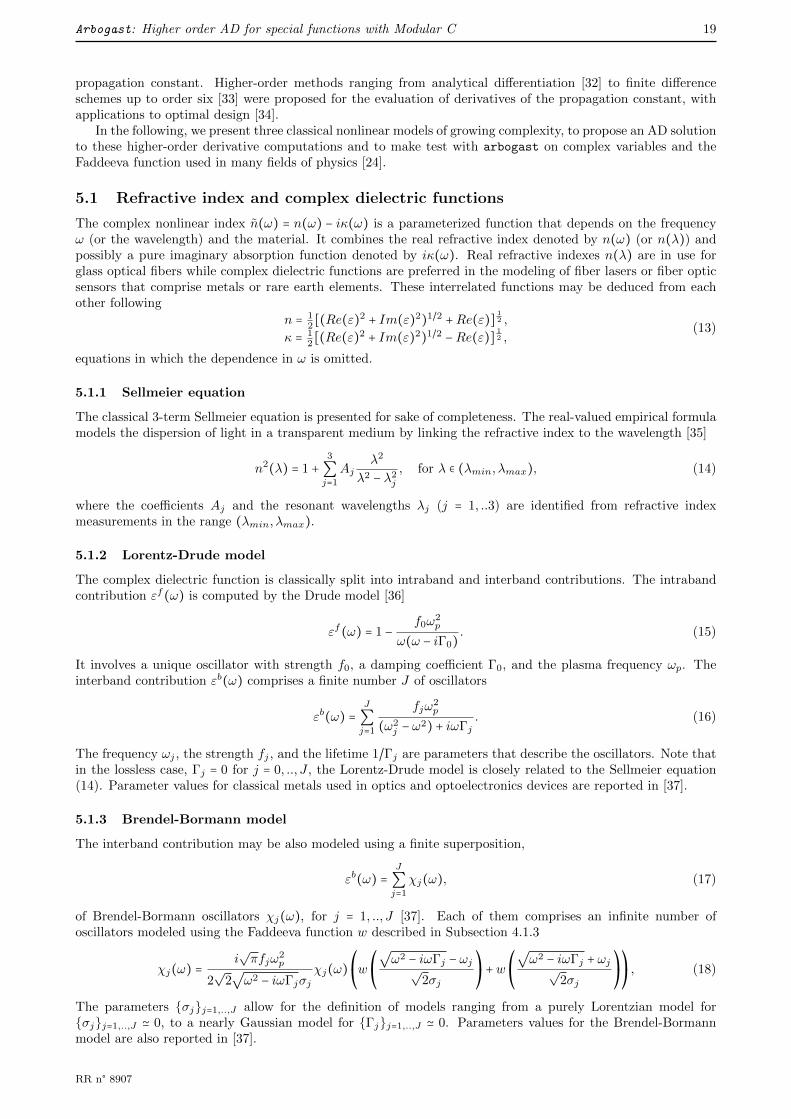
Arbogast: Higher order AD for special functions with Modular C 19
propagation constant. Higher-order methods ranging from analytical differentiation [32] to finite differenceschemes up to order six [33] were proposed for the evaluation of derivatives of the propagation constant, withapplications to optimal design [34].
In the following, we present three classical nonlinear models of growing complexity, to propose an AD solutionto these higher-order derivative computations and to make test with arbogast on complex variables and theFaddeeva function used in many fields of physics [24].
5.1 Refractive index and complex dielectric functions
The complex nonlinear index n(ω) = n(ω) − iκ(ω) is a parameterized function that depends on the frequencyω (or the wavelength) and the material. It combines the real refractive index denoted by n(ω) (or n(λ)) andpossibly a pure imaginary absorption function denoted by iκ(ω). Real refractive indexes n(λ) are in use forglass optical fibers while complex dielectric functions are preferred in the modeling of fiber lasers or fiber opticsensors that comprise metals or rare earth elements. These interrelated functions may be deduced from eachother following
n = 12[(Re(ε)2 + Im(ε)2)1/2 +Re(ε)]
12 ,
κ = 12[(Re(ε)2 + Im(ε)2)1/2 −Re(ε)]
12 ,
(13)
equations in which the dependence in ω is omitted.
5.1.1 Sellmeier equation
The classical 3-term Sellmeier equation is presented for sake of completeness. The real-valued empirical formulamodels the dispersion of light in a transparent medium by linking the refractive index to the wavelength [35]
n2(λ) = 1 +3
∑j=1
Ajλ2
λ2 − λ2j, for λ ∈ (λmin, λmax), (14)
where the coefficients Aj and the resonant wavelengths λj (j = 1, ..3) are identified from refractive indexmeasurements in the range (λmin, λmax).
5.1.2 Lorentz-Drude model
The complex dielectric function is classically split into intraband and interband contributions. The intrabandcontribution εf(ω) is computed by the Drude model [36]
εf(ω) = 1 −f0ω
2p
ω(ω − iΓ0). (15)
It involves a unique oscillator with strength f0, a damping coefficient Γ0, and the plasma frequency ωp. Theinterband contribution εb(ω) comprises a finite number J of oscillators
εb(ω) =J
∑j=1
fjω2p
(ω2j − ω
2) + iωΓj. (16)
The frequency ωj , the strength fj , and the lifetime 1/Γj are parameters that describe the oscillators. Note thatin the lossless case, Γj = 0 for j = 0, .., J , the Lorentz-Drude model is closely related to the Sellmeier equation(14). Parameter values for classical metals used in optics and optoelectronics devices are reported in [37].
5.1.3 Brendel-Bormann model
The interband contribution may be also modeled using a finite superposition,
εb(ω) =J
∑j=1
χj(ω), (17)
of Brendel-Bormann oscillators χj(ω), for j = 1, .., J [37]. Each of them comprises an infinite number ofoscillators modeled using the Faddeeva function w described in Subsection 4.1.3
χj(ω) =i√πfjω
2p
2√
2√ω2 − iωΓjσj
χj(ω)⎛
⎝w
⎛
⎝
√ω2 − iωΓj − ωj
√2σj
⎞
⎠+w
⎛
⎝
√ω2 − iωΓj + ωj
√2σj
⎞
⎠
⎞
⎠, (18)
The parameters {σj}j=1,..,J allow for the definition of models ranging from a purely Lorentzian model for{σj}j=1,..,J ≃ 0, to a nearly Gaussian model for {Γj}j=1,..,J ≃ 0. Parameters values for the Brendel-Bormannmodel are also reported in [37].
RR n° 8907
Arbogast: Higher order AD for special functions with Modular C 20
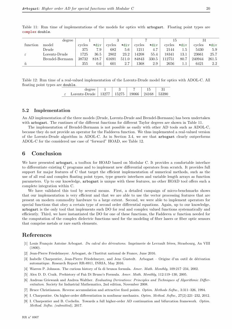
Table 11: Run time of implementations of the models for optics with arbogast. Floating point types arecomplex double.
degree 1 3 7 15 31function model cycles *div cycles *div cycles *div cycles *div cycles *div
Drude 375 7.9 682 5.6 1211 4.7 2144 1.5 5430 5.9ε Lorentz-Drude 1725 36.5 2802 23.2 14208 55.4 18341 13.1 23661 25.7
Brendel-Bormann 38732 818.7 61691 511.0 84843 330.5 112751 80.7 240944 261.5n 355 0.6 601 2.7 1368 2.9 2656 1.1 6421 2.2
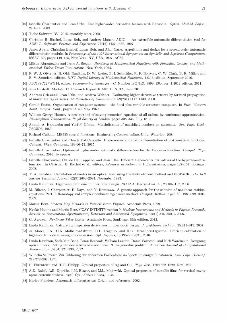
Table 12: Run time of a real-valued implementation of the Lorentz-Drude model for optics with ADOL-C. Allfloating point types are double.
degree 1 3 7 15 31ε Lorentz-Drude 13277 15275 19066 24168 53390
5.2 Implementation
An AD implementation of the three models (Drude, Lorentz-Drude and Brendel-Bormann) has been undertakenwith arbogast. The runtimes of the different functions for different Taylor degrees are shown in Table 11.
The implementation of Brendel-Bormann is not possible as easily with other AD tools such as ADOL-C,because they do not provide an operator for the Faddeeva function. We thus implemented a real-valued versionof the Lorentz-Drude algorithm in ADOL-C. As in Section 3.4, we see that arbogast clearly outperformsADOL-C for the considered use case of “forward” HOAD, see Table 12.
6 Conclusion
We have presented arbogast, a toolbox for HOAD based on Modular C. It provides a comfortable interfaceto differentiate existing C programs and to implement new differential operators from scratch. It provides fullsupport for major features of C that target the efficient implementation of numerical methods, such as theuse of all real and complex floating point types, type generic interfaces and variable length arrays as functionparameters. Up to our knowledge, arbogast is unique with these features, no other HOAD tool offers such acomplete integration within C.
We have validated this tool by several means. First, a detailed campaign of micro-benchmarks showsthat our implementation is very efficient and that we are able to use the vector processing features that arepresent on modern commodity hardware to a large extent. Second, we were able to implement operators forspecial functions that obey a certain type of second order differential equations. Again, up to our knowledge,arbogast is the only tool that implements such DO for real and complex valued functions systematically andefficiently. Third, we have instantiated the DO for one of these functions, the Faddeeva w function needed forthe computation of the complex dielectric functions used for the modeling of fiber lasers or fiber optic sensorsthat comprise metals or rare earth elements.
References
[1] Louis Francois Antoine Arbogast. Du calcul des derivations. Imprimerie de Levrault freres, Strasbourg, An VIII(1800).
[2] Jean-Pierre Friedelmeyer. Arbogast, de l’Institut national de France, June 2016.
[3] Isabelle Charpentier, Jean-Pierre Friedelmeyer, and Jens Gustedt. Arbogast – Origine d’un outil de derivationautomatique. Research Report RR-8911, INRIA, May 2016.
[4] Warren P. Johnson. The curious history of fa di brunos formula. Amer. Math. Monthly, 109:217–234, 2002.
[5] Alex D. D. Craik. Prehistory of Faa Di Bruno’s Formula. Amer. Math. Monthly, 112:119–130, 2005.
[6] Andreas Griewank and Andrea Walther. Evaluating Derivatives: Principles and Techniques of Algorithmic Differ-entiation. Society for Industrial Mathematics, 2nd edition, November 2008.
[7] Bruce Christianson. Reverse accumulation and attractive fixed points. Optim. Methods Softw., 3:311–326, 1994.
[8] I. Charpentier. On higher-order differentiation in nonlinear mechanics. Optim. Method. Softw., 27(2):221–232, 2012.
[9] I. Charpentier and B. Cochelin. Towards a full higher-order AD continuation and bifurcation framework. Optim.Method. Softw. (submitted), 2017.
RR n° 8907
Arbogast: Higher order AD for special functions with Modular C 21
[10] Isabelle Charpentier and Jean Utke. Fast higher-order derivative tensors with Rapsodia. Optim. Method. Softw.,24:1–14, 2009.
[11] Tiobe Software BV, 2015. monthly since 2000.
[12] Christian H. Bischof, Lucas Roh, and Andrew Mauer. ADIC — An extensible automatic differentiation tool forANSI-C. Software–Practice and Experience, 27(12):1427–1456, 1997.
[13] Jason Abate, Christian Bischof, Lucas Roh, and Alan Carle. Algorithms and design for a second-order automaticdifferentiation module. In Proceedings of the 1997 International Symposium on Symbolic and Algebraic Computation,ISSAC ’97, pages 149–155, New York, NY, USA, 1997. ACM.
[14] Milton Abramowitz and Irene A. Stegun. Handbook of Mathematical Functions with Formulas, Graphs, and Math-ematical Tables. Dover Publications, New York, 1964.
[15] F. W. J. Olver, A. B. Olde Daalhuis, D. W. Lozier, B. I. Schneider, R. F. Boisvert, C. W. Clark, B. R. Miller, andB. V. Saunders, editors. NIST Digital Library of Mathematical Functions. 1.0.13 edition, September 2016.
[16] JTC1/SC22/WG14, editor. Programming languages - C. Number ISO/IEC 9899. ISO, cor. 1:2012 edition, 2011.
[17] Jens Gustedt. Modular C. Research Report RR-8751, INRIA, June 2015.
[18] Andreas Griewank, Jean Utke, and Andrea Walther. Evaluating higher derivative tensors by forward propagationof univariate taylor series. Mathematics of Computation, 69(231):1117–1130, 2000.
[19] Gerald Estrin. Organization of computer systems – the fixed plus variable structure computer. In Proc. WesternJoint Comput. Conf., pages 33–40, May 1960.
[20] William George Horner. A new method of solving numerical equations of all orders, by continuous approximation.Philosophical Transactions. Royal Society of London, pages 308–335, July 1819.
[21] Anatoli A. Karatsuba and Yuri P. Ofman. Multiplication of multidigit numbers on automata. Sov. Phys. Dokl.,7:595596, 1963.
[22] Richard Culham. ME755 special functions. Engineering Courses online, Univ. Waterloo, 2004.
[23] Isabelle Charpentier and Claude Dal Cappello. Higher-order automatic differentiation of mathematical functions.Comput. Phys. Commun., 189:66–71, 2015.
[24] Isabelle Charpentier. Optimized higher-order automatic differentiation for the Faddeeva function. Comput. Phys.Commun., 2016. to appear.
[25] Isabelle Charpentier, Claude Dal Cappello, and Jean Utke. Efficient higher-order derivatives of the hypergeometricfunction. In Christian H. Bischof et al., editors, Advances in Automatic Differentiation, pages 127–137. Springer,2008.
[26] T. A. Lenahan. Calculation of modes in an optical fiber using the finite element method and EISPACK. The BellSystem Technical Journal, 62(9):2663–2694, November 1983.
[27] Linda Kaufman. Eigenvalue problems in fiber optic design. SIAM J. Matrix Anal. A., 28:105–117, 2006.
[28] M. Bilasse, I. Charpentier, E. Daya, and Y. Koutsawa. A generic approach for the solution of nonlinear residualequations. Part II: Homotopy and complex nonlinear eigenvalue method. Comput. Method. Appl. M., 198:3999–4004,2009.
[29] Martin Berz. Modern Map Methods in Particle Beam Physics. Academic Press, 1999.
[30] Kyoko Makino and Martin Berz. COSY INFINITY version 9. Nuclear Instruments and Methods in Physics Research,Section A: Accelerators, Spectrometers, Detectors and Associated Equipment, 558(1):346–350, 3 2006.
[31] G. Agrawal. Nonlinear Fiber Optics. Academic Press, SanDiego, fifth edition, 2012.
[32] Linda Kaufman. Calculating dispersion derivatives in fiber-optic design. J. Lightwave Technol., 25:811–819, 2007.
[33] Jr. Mores, J.A., G.N. Malheiros-Silveira, H.L. Fragnito, and H.E. Hernandez-Figueroa. Efficient calculation ofhigher-order optical waveguide dispersion. Opt. Express, 18:19522–19531, 2010.
[34] Linda Kaufman, Seok-Min Bang, Brian Heacook, William Landon, Daniel Savacool, and Nick Woronekin. Designingoptical fibers: Fitting the derivatives of a nonlinear PDE-eigenvalue problem. American Journal of ComputationalMathematics, 02(04):321–330, 2012.
[35] Wilhelm Sellmeier. Zur Erklarung der abnormen Farbenfolge im Spectrum einiger Substanzen. Ann. Phys. (Berlin),219:272–282, 1871.
[36] H. Ehrenreich and H. R. Philipp. Optical properties of Ag and Cu. Phys. Rev., 128:1622–1629, Nov 1962.
[37] A.D. Rakic, A.B. Djurisic, J.M. Elazar, and M.L. Majewski. Optical properties of metallic films for vertical-cavityoptoelectronic devices. Appl. Opt., 37:5271–5283, 1998.
[38] Harley Flanders. Automatic differentiation: Origin and references, 2002.
RR n° 8907

RESEARCH CENTRENANCY – GRAND EST
615 rue du Jardin BotaniqueCS2010154603 Villers-lès-Nancy Cedex
PublisherInriaDomaine de Voluceau - RocquencourtBP 105 - 78153 Le Chesnay Cedexinria.fr
ISSN 0249-6399