Architecture 4.411 Building Technology Laboratory Spring 2004

Tutorial and design exercises for airflow studies using CONTAMW 2.0

Buoyancy-driven flows

Please complete Table 1, using Table 2 as a template. It is not necessary to fill in all rows, but please provide a reasonable set of cases.

Single-zone base case

Open CONTAMW 2.0.

Create a single-zone building by drawing a box or, alternatively, four walls

Define an indoor zone by right clicking inside the box to reveal the icon pull-down menu, then selecting zone.

Double click on the icon, name the zone and assign a volume, floor area, and indoor temperature. Note that the floor area and volume are automatically related by an assumed height of 3 meters. You can change this value by opening the Level pull-down menu and selecting Edit Level Data.

Save your project before going too far.

Right click somewhere on the perimeter – say, the upper wall – and select flow path.

Double click to define the properties for the airflow path. First, select a flow element. n∆Click the New Element tab and try the power law for volumetric flow, Q = P C . Name

this element (inlet, perhaps). The flow exponent is fine as is, at 0.5, but the flow coefficient needs to account for the area of the window. Let the flow coefficient be the

window area in m2, multiplied by 0.77. The factor of 0.77 is Cd 2 , where the discharge ρ

coefficient is 0.6 and the density is 1.2 kg/m3. Try 1 m2 for now, which means the flow coefficient should be 0.77. Then select the flow path tab and give the window a height relative to the floor. The default of 1.5 m is fine, for starters.

Right click again on the perimeter to design a second flow path, on the lower wall. Repeat the process above to define its properties. Call the flow element “outlet.” Keep the default height of 1.5 m. Save your file.

1

Select the weather pull-down menu and note that the ambient temperature is 20 oC.

Open the simulation pull-down menu, run the simulation and note that nothing changes on the sketch pad. Click on either of the openings and note that the flow reported at the bottom of the CONTAMW window is zero. Open the simulation pull-down menu again, export the data as a text file, open the file, and note that there is no flow. Why? Think carefully: there are two reasons.

Change the ambient temperature to 15 oC and try again. Still no airflow. Don’t bother with exporting data. When the sketch pad is unchanged, there will be no data.

Now double click on the icon for the second flow path, click on the flow-path button, and change the relative height to 3 m. Again, run the simulation. Does the sketch pad change? It does. There are blue lines for flows and red lines for pressures. Note that the flows and pressures are the same for both openings. The direction of the lines differs: the set for the inlet points into the indoor zone and the set for the outlet points outward, denoting the flow direction. Export the data, open the data file, and note that the flows, in sm3/hr, are indeed equal and opposite in sign. The units are standard m3/hr, which account for the changes in temperature and therefore density. Standard volumetric flow is conserved, as is mass flow. Jot down the value for the flow and, even better, divide by the volume to obtain an air-change-per-hour value. Note also the indoor pressure relative to ambient and the pressure differences across the openings.

While this tutorial will continue with changes to window height, you may at times want to add a new opening. In this case, you must pull down the View menu and turn off the sketchpad results to return to the normal sketchpad mode.

Does height matter?

Increase the height of the outlet to 4.5 m and re-run the simulation. Jot down the results. You have now doubled the height between the inlet and outlet windows. Does the airflow double? More than double? Less than double? Try a few more heights and tabulate the results. Plot or sketch the relation between airflow and height. Is a larger stack (chimney, stairwell, atrium) a good idea?

Does temperature difference matter?

Increase the temperature difference, by either warming the indoors or dropping the outdoor temperature. Try a few values of temperature difference. How does flow vary with temperature difference? Does it matter whether it is 25 oC in and 15 out, or 20 oC in and 10 out, both with a temperature difference of 10 oC? If it does matter, is the effect large or small?

What does this say about solar chimneys or using heat gains in a double-façade cavity to draw air through occupied spaces?

2

Does window size matter?

Double the area of both the inlet and the outlet. What do you expect to happen to the airflow? What does happen?

Now fix the total window area but make the two openings unequal. Start with a small inlet and a large outlet. Note the airflows and pressures. Flip things around and make a small inlet and a large outlet. Compare.

3

Wind-driven flows

Please complete Table 3, using Table 4 as an example.

Single-zone base case

Now let’s modify the same model to examine wind-driven flows. Set the height of the inlet and outlet windows to the same value. Ditto with the indoor and outdoor temperatures.

Constant wind pressure

Let’s deal with the wind in increasingly more realistic ways. First, for the inlet window define a constant wind pressure of 0.6 Pa, which corresponds to a 1 m/s wind. For the outlet, define the wind pressure as -0.6 Pa. Re-run the simulation and note, not surprisingly, that you obtain a flow. How does the value compare with those you obtained from buoyancy effects?

If you prefer to estimate airflows due to a 2 m/s wind, please keep in mind that the wind pressure varies with the square of the wind speed and set the wind pressures to 2.4 Pa and -2.4 Pa. How does the airflow compare with what you calculated for 1 m/s? It doubles. Why, given what we did to the wind pressures? Because flow through an opening varies with the square root of the pressure drop across the opening.

Here’s something else. Take the airflow for the wind pressure that corresponds to 1 m/s. Divide by 3600 to get m3/s. Recall that the window opening has a flow coefficient of 0.77, which corresponds to an opening area of 1 m2/s. Divide the airflow in m3/s by 1 m2

of area to obtain the speed of the air through the opening. How does it compare to the wind speed of 1 m/s? If you try the same procedure for higher wind pressures, you should obtain the same ratio, approximately 0.5. This is worth remembering, even if it only holds true when the windows are the same size and wind pressures are equal in magnitude and opposite in sign. It gives us an idea of wind speed indoors, where a value greater than about 2 m/s can cause papers to blow.

Variable wind pressure

Now, consider a second, more complex but more realistic way of dealing with the wind. The first method is indeed easy but requires the user to input the wind pressures. We would prefer not to do that. What we would like is to specify a wind speed and direction and let the simulation handle the rest.

Double click on the inlet opening, click on the wind tab, then change the wind-pressure option to variable. We now need to consider a wind-speed multiplier, a wall azimuth angle, and a wind-pressure profile. The azimuth angle is easy. For the inlet, set it to 0

4

degrees, meaning that the upper wall faces the north. For the outlet window, be sure to set the azimuth to 180 degrees.

The other two issues are harder but necessarily so. They say a lot about wind speed at the building and how wind pressures vary on different surfaces of the building. Both are important.

Wind-speed multiplier

We are accustomed to saying that the outdoor wind speed has a certain value. TV weather forecasters cite values, as do on-line weather services. What do these numbers really mean? If you went outside whatever building you happened to be in, would you measure the same value? Probably not.

Wind speeds in weather files and reports are typically measured at airports, at a height of 10 m. They are lower than free-stream values at higher elevations, entirely uninfluenced by the boundary layer right at the surface of the earth. The boundary layer is the same sort of deal that gives windows their thermal resistance, but at a larger scale. We know they exist: if you were an ant you would experience very little wind. If you are in the upper floor of a skyscraper – say on the observation deck of the Empire State Building – you would find it much windier than at ground level. This phenomenon, by the way, is what has partially motivated double-skin facades for tall buildings.

If you stop to think about it, you would expect the wind-speed multiplier to be a fraction less than one and would further expect it to depend on two factors: height and terrain. For very open terrain, say on a beach or at an airport, the wind speed picks up relatively rapidly with height. For urban areas, buildings obstruct and reduce the wind speed.

Open the weather pull-down menu, edit the wind and weather data, and take a look at the wind tab. Note that there is opportunity to specify wall height. The default terrain constant (0.6) and the velocity profile exponent (0.28) are appropriate for suburban buildings. See the ASHRAE Handbook of Fundamentals (what else?) or, more directly, pages 99-100 of the CONTAMW manual for values suitable for urban or open terrain. CONTAMW calculates the wind-pressure modifier and inserts it into the description of the flow path. You can change it, of course, but there should be no need to second guess the program.

Wind-pressure profiles

Hold your hand out of a car window while moving at high speed, with your palms and fingers perpendicular to the ground. The rushing air tends to push your hand back. Rotate your hand 90 degrees and note how much less pressure you feel. The pressure on your hand increases with the square of the wind speed, as noted above, which is why raising speed limits reduces fuel economy. It is also why tractor-trailer rigs have a wind deflector above the cab.

5

Cars are judged to be aerodynamic if they have a low drag coefficient. True as far as it goes. However, the wind pressure on a car is the product of the square of the wind speed, the drag coefficient, and the cross-sectional area. A sports car may have a drag coefficient larger than a sedan but still face lower air resistance, because its cross-sectional area is much smaller.

For buildings, wind-pressure coefficients are the means by which we assess how easily wind flows around or over a building. As a hypothetical case, consider the wind hitting a very large wall. Imagine you are at the center point of the wall. You would feel pretty much the full brunt of the wind. Assign a wind-pressure coefficient of 1.0 to this point. Now, continuing the hypothetical case, go to the back side of the building under the same circumstances. Now you would feel a certain pull away from the wall, a negative pressure that tends to draw air out of a building. Assign a wind-pressure coefficient of -1.0 to this point.

In CONTAMW, we can do just this by creating a wind-pressure profile. Try it! Double-click on the inlet, click on the wind-pressure tab, select variable wind pressure, and then select a new profile. You need only assign values to 0, 180 and 360 degrees: 1, -1, and 1. Give the profile a name of your choice. Now work on the outlet, and notice that your new profile is available for this window as well. No need to start over! If you want to save it for use with other CONTAMW projects, you can create a library and add the profile to it. Easy and handy.

Open the weather menu and set the wind speed to 2 m/s, with a wind direction of 0 degrees. Run the simulation and examine the results. Note that the airflow is less than what you obtained by setting the wind-pressure coefficients to 2.4 and -2.4. Why? Because the wind-speed multiplier is less than 1.0. In fact, if you take the airflow obtained for a 2 m/s wind and wind pressures of 2.4 and -2.4 and multiply by the square root of the wind-pressure coefficient, you should obtain the airflow for a more reasonable estimate of wind speed at the building. See Table 3 for my results.

Our very simple wind-pressure profile is of little practical use. It is not reasonable for anything but both sides of a near-infinite wall, with the wind smacking into one side head-on. Real buildings have four walls (or more) and roofs. Roofs may rest on gabled walls. Wind strikes buildings at different angles.

To deal with these complexities, CONTAMW allows us to select a wind-pressure profile. Get back into the wind-pressure tab under airflow path properties (i.e., double-click on the inlet icon), click on library, then browse and open WNDPRS.LB2. There is a bewildering array of choices. Try looking at a couple. Note the differences between roof and wall profiles. Select something like S&C_1_Both. Now re-run the simulation and note the decrease in airflow because the wind is not beating against the building as hard as it would against a very large wall.

Change the wind direction to 45 and notice a flow smaller than what you recorded when the wind was a 0 degrees. Change the wind direction to 90 degrees. Any flow? No.

6

While the wind-pressure profile shows a suction when the wind is parallel to the wall, the two windows are on opposite sides of the building and feel the same suction. No air goes in, no air goes out.

Two windows on same side, no other openings

Create a new model. You can use the Save As command for this reason. Move the outlet window to the upper (north) wall. Keep the heights of both at the same value. Run the simulation. Any airflow? Shouldn’t be, and there is not. The wind is pushing against both windows, there is no place for air to come out, and there is no flow.

Now change the height of one of the windows. Change it substantially if you like. Any flow? The simulation reports none. What do you expect? If one window were much higher than the other, you might expect the larger wind speed at the higher elevation to have a higher pressure, and force some air in that would come out at the lower elevation. CONTAMW uses the height of the wall, and not each window, to calculate wind speed and takes it to be the same for all windows. The wind-speed multiplier can be changed for each window, and relatively easily, but let’s pass on that for now.

7

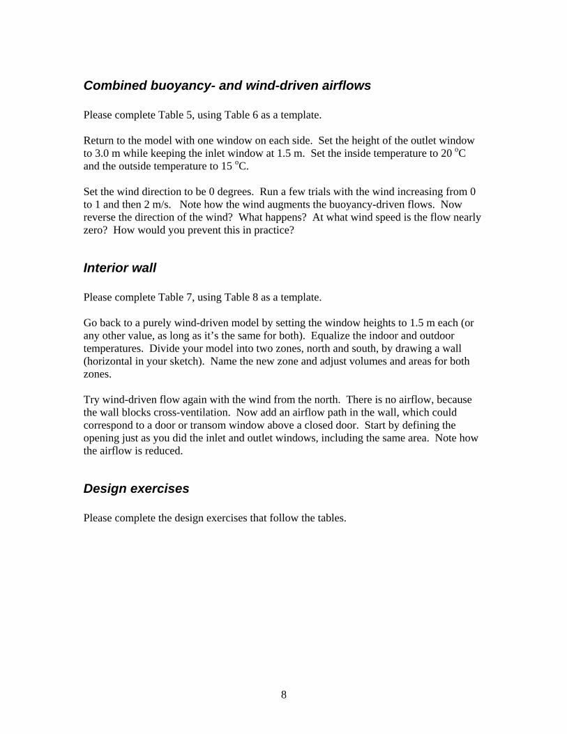
Combined buoyancy- and wind-driven airflows

Please complete Table 5, using Table 6 as a template.

Return to the model with one window on each side. Set the height of the outlet window to 3.0 m while keeping the inlet window at 1.5 m. Set the inside temperature to 20 oC and the outside temperature to 15 oC.

Set the wind direction to be 0 degrees. Run a few trials with the wind increasing from 0 to 1 and then 2 m/s. Note how the wind augments the buoyancy-driven flows. Now reverse the direction of the wind? What happens? At what wind speed is the flow nearly zero? How would you prevent this in practice?

Interior wall

Please complete Table 7, using Table 8 as a template.

Go back to a purely wind-driven model by setting the window heights to 1.5 m each (or any other value, as long as it’s the same for both). Equalize the indoor and outdoor temperatures. Divide your model into two zones, north and south, by drawing a wall (horizontal in your sketch). Name the new zone and adjust volumes and areas for both zones.

Try wind-driven flow again with the wind from the north. There is no airflow, because the wall blocks cross-ventilation. Now add an airflow path in the wall, which could correspond to a door or transom window above a closed door. Start by defining the opening just as you did the inlet and outlet windows, including the same area. Note how the airflow is reduced.

Design exercises

Please complete the design exercises that follow the tables.

8

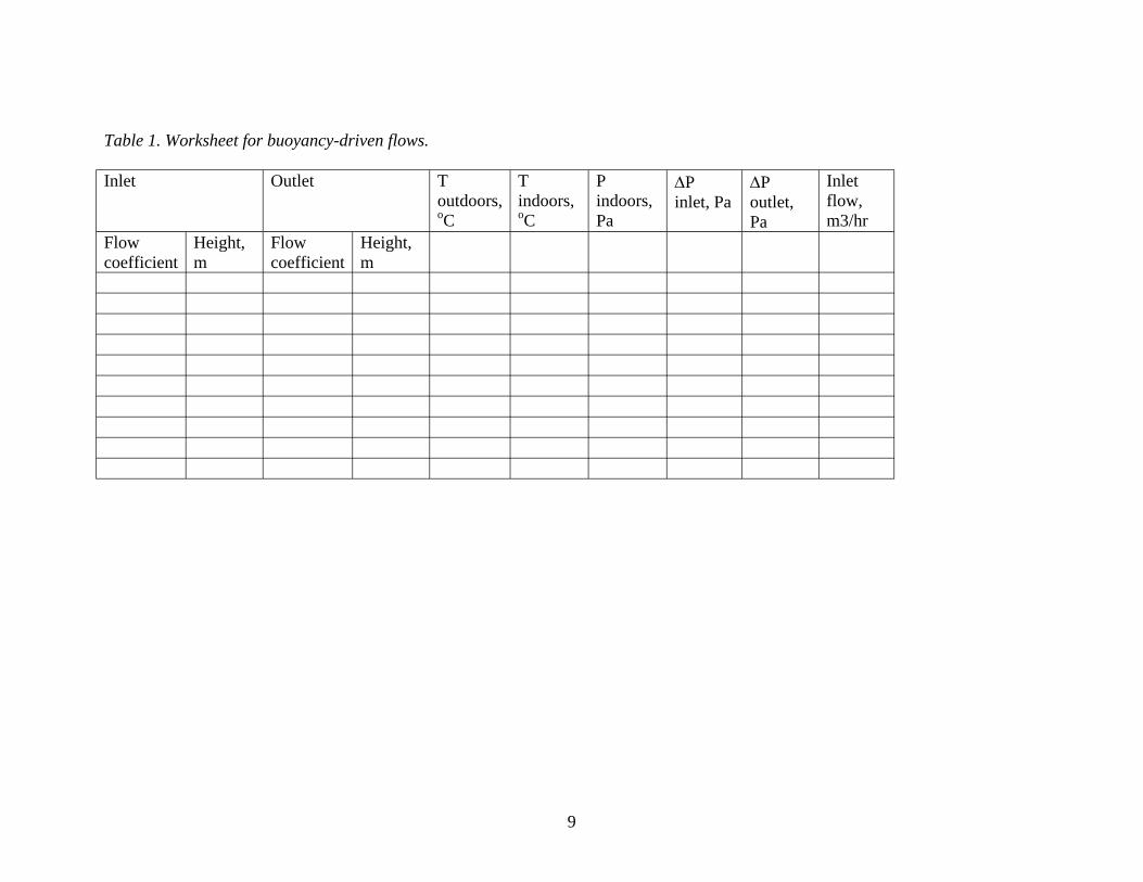
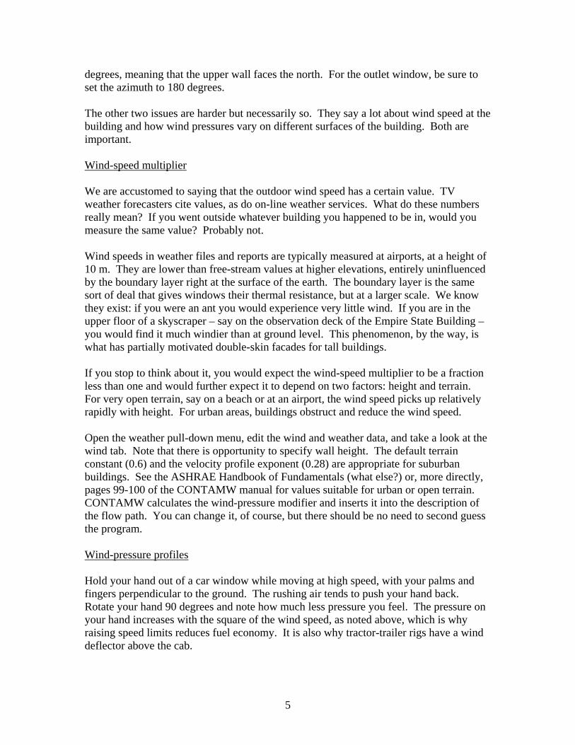
Table 1. Worksheet for buoyancy-driven flows.

Inlet Outlet T T P ∆P ∆P Inlet outdoors, indoors, indoors, inlet, Pa outlet, flow, oC oC Pa Pa m3/hr

Flow Height, Flow Height, coefficient m coefficient m

9

Table 2. Examples of buoyancy-driven flows.

Inlet Outlet T T P ∆P ∆P Inlet outdoors, oC

indoors, oC

indoors, Pa

inlet, Pa outlet, Pa

flow, m3/hr

Flow Height, Flow Height, coefficient m coefficient m 0.77 1.5 0.77 1.5 20 20 0.0 0.0 0.0 0 0.77 1.5 0.77 1.5 15 20 0.0 0.0 0.0 0 0.77 1.5 0.77 3.0 15 20 -0.5 0.2 -0.2 1096 0.77 1.5 0.77 4.5 15 20 -0.6 0.3 -0.3 1550 0.77 1.5 0.77 6.0 15 20 -0.8 0.5 -0.5 1898 0.77 1.5 0.77 3.0 15 25 -0.9 0.3 -0.3 1523 0.77 1.5 0.77 3.0 10 20 -0.9 0.3 -0.3 1577 1.54 1.5 1.54 3.0 15 20 -0.5 0.2 -0.2 2191 0.77 1.5 2.31 3.0 15 20 -0.6 0.3 0 1480 2.31 1.5 0.77 3.0 15 20 -0.3 0 -0.3 1460

10

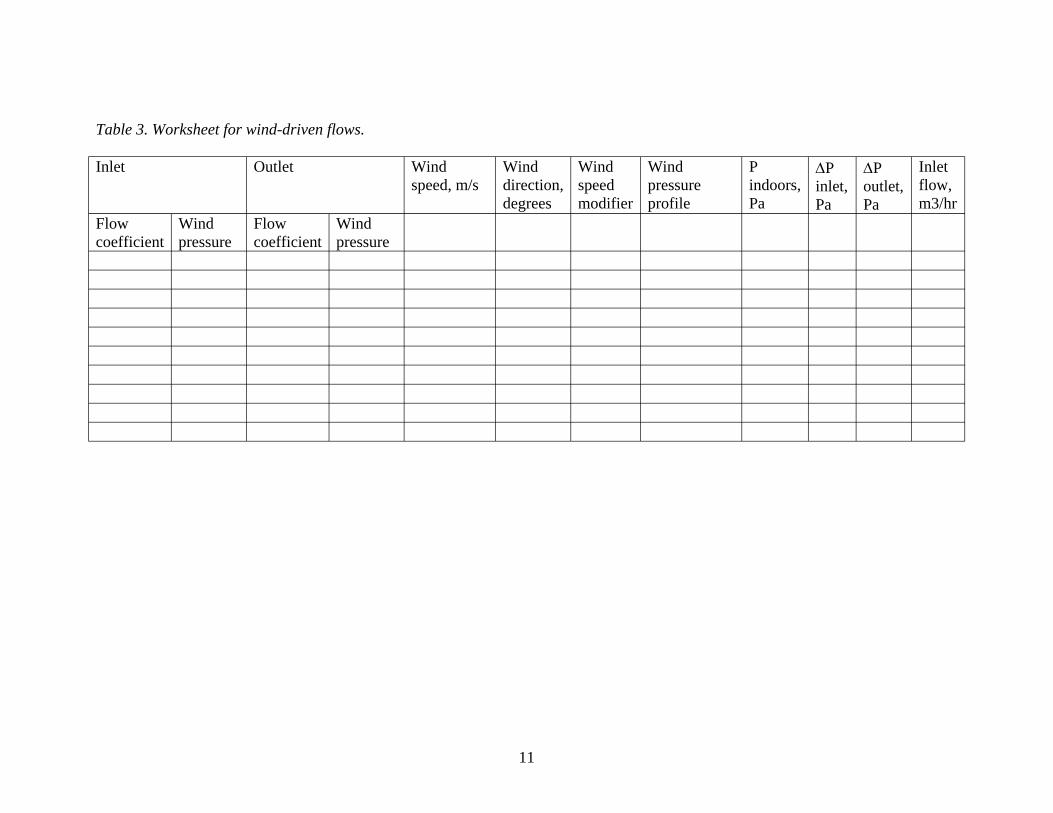
Table 3. Worksheet for wind-driven flows.

Inlet Outlet Wind Wind Wind Wind P ∆P ∆P Inlet speed, m/s direction, speed pressure indoors, inlet, outlet, flow,

degrees modifier profile Pa Pa Pa m3/hr Flow coefficient

Wind pressure

Flow coefficient

Wind pressure

11

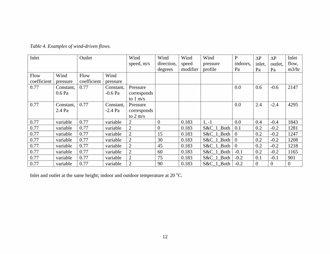
Table 4. Examples of wind-driven flows.

Inlet Outlet Wind Wind Wind Wind P ∆P ∆P Inlet speed, m/s direction, speed pressure indoors, inlet, outlet, flow,

degrees modifier profile Pa Pa Pa m3/hr Flow coefficient

Wind pressure

Flow coefficient

Wind pressure

0.77 Constant, 0.77 Constant, Pressure 0.0 0.6 -0.6 2147 0.6 Pa -0.6 Pa corresponds

to 1 m/s 0.77 Constant, 0.77 Constant, Pressure 0.0 2.4 -2.4 4295

2.4 Pa -2.4 Pa corresponds to 2 m/s

0.77 variable 0.77 variable 2 0 0.183 1, -1 0.0 0.4 -0.4 1843 0.77 variable 0.77 variable 2 0 0.183 S&C_1_Both 0.1 0.2 -0.2 1281 0.77 variable 0.77 variable 2 15 0.183 S&C_1_Both 0 0.2 -0.2 1247 0.77 variable 0.77 variable 2 30 0.183 S&C_1_Both 0 0.2 -0.2 1208 0.77 variable 0.77 variable 2 45 0.183 S&C_1_Both 0 0.2 -0.2 1218 0.77 variable 0.77 variable 2 60 0.183 S&C_1_Both -0.1 0.2 -0.2 1165 0.77 variable 0.77 variable 2 75 0.183 S&C_1_Both -0.2 0.1 -0.1 901 0.77 variable 0.77 variable 2 90 0.183 S&C_1_Both -0.2 0 0 0

Inlet and outlet at the same height; indoor and outdoor temperature at 20 oC.

12

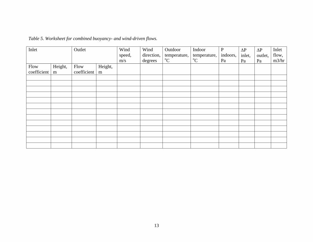
Table 5. Worksheet for combined buoyancy- and wind-driven flows.

Inlet Outlet Wind Wind Outdoor Indoor P ∆P ∆P Inlet speed, direction, temperature, temperature, indoors, inlet, outlet, flow, m/s degrees oC oC Pa Pa Pa m3/hr

Flow Height, Flow Height, coefficient m coefficient m

13

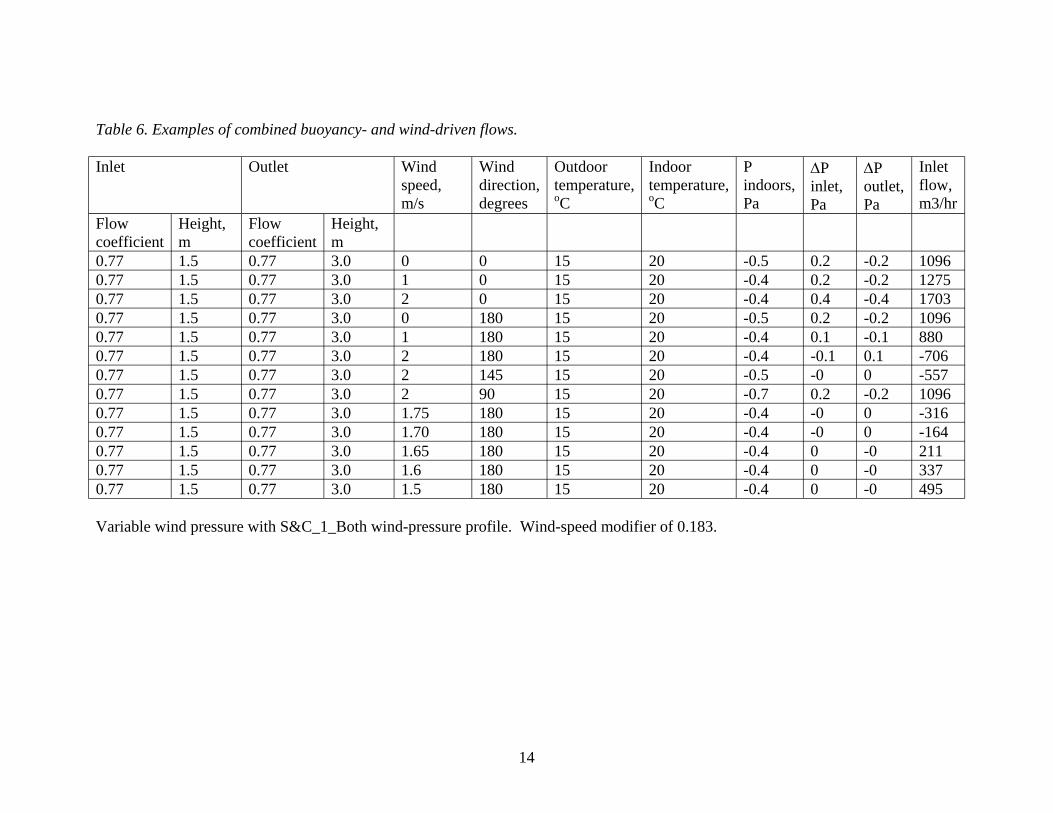
Table 6. Examples of combined buoyancy- and wind-driven flows.

Inlet Outlet Wind Wind Outdoor Indoor P ∆P ∆P Inlet speed, direction, temperature, temperature, indoors, inlet, outlet, flow, m/s degrees oC oC Pa Pa Pa m3/hr

Flow Height, Flow Height, coefficient m coefficient m 0.77 1.5 0.77 3.0 0 0 15 20 -0.5 0.2 -0.2 1096 0.77 1.5 0.77 3.0 1 0 15 20 -0.4 0.2 -0.2 1275 0.77 1.5 0.77 3.0 2 0 15 20 -0.4 0.4 -0.4 1703 0.77 1.5 0.77 3.0 0 180 15 20 -0.5 0.2 -0.2 1096 0.77 1.5 0.77 3.0 1 180 15 20 -0.4 0.1 -0.1 880 0.77 1.5 0.77 3.0 2 180 15 20 -0.4 -0.1 0.1 -706 0.77 1.5 0.77 3.0 2 145 15 20 -0.5 -0 0 -557 0.77 1.5 0.77 3.0 2 90 15 20 -0.7 0.2 -0.2 1096 0.77 1.5 0.77 3.0 1.75 180 15 20 -0.4 -0 0 -316 0.77 1.5 0.77 3.0 1.70 180 15 20 -0.4 -0 0 -164 0.77 1.5 0.77 3.0 1.65 180 15 20 -0.4 0 -0 211 0.77 1.5 0.77 3.0 1.6 180 15 20 -0.4 0 -0 337 0.77 1.5 0.77 3.0 1.5 180 15 20 -0.4 0 -0 495

Variable wind pressure with S&C_1_Both wind-pressure profile. Wind-speed modifier of 0.183.

14

Table 7. Worksheet for interior openings.

Inlet Outlet Interior P ∆P P ∆P Flow, zone 1, inlet, zone 2, outlet, m3/hr Pa Pa Pa Pa

Flow Height, Flow Height, Flow Height, coefficient m coefficient m coefficient m

15

Table 8. Examples of interior openings.

Inlet Outlet Interior P ∆P P ∆P Flow, zone 1, inlet, zone 2, outlet, m3/hr Pa Pa Pa Pa

Flow Height, Flow Height, Flow Height, coefficient m coefficient m coefficient m 0.77 1.5 0.77 1.5 0.77 1.5 0.1 0.1 -0 -0.1 1046 0.77 1.5 0.77 1.5 1.54 1.5 0.1 0.2 0 -0.2 1208 0.77 1.5 0.77 1.5 2.31 1.5 0.1 0.2 0 -0.2 1247

Variable wind pressure with S&C_1_Both wind-pressure profile. Wind-speed modifier of 0.183.

16

Design exercises with CONTAMW

Buoyancy-driven flows in an auditorium

Consider buoyancy driven airflow in an auditorium. The space is 400 m2 and is occupied by 200 people. Assume the walls adjoin other spaces and that there is no conduction across them. Further assume that each person emits 75 W of heat and that lighting power is 15 W/m2. Establish several possible combinations of opening areas and height of a ventilation chimney that will maintain the indoor temperature at 5 oC above the outdoor temperature. Proceed as follows in CONTAMW:

Define a single-zone building and two openings, inlet and outlet.

Pick a comfortable indoor temperature. Select the outdoor temperature as 5 oC lower.

Pick what you consider to be reasonable opening areas and a reasonable height differential between inlet and outlet.

Calculate the volumetric flow, in m3/hr.

Calculate the heat flow associated with this flow, by multiplying the flow by the density of air, its heat capacity, and the temperature difference.

q = ρ ⋅C p ⋅V ⋅ (T −Tout )in

where

ρ = density of air, 1.2 kg/m3

Cp = specific heat of air, 1000 J/kg oC V = flow rate, m3/s

If the heat flow matches that generated by lights and occupants, you have an acceptable design. If not, you will need to increase or decrease the window openings or the height between them.

Repeat the process to investigate how you can trade off window size against height. Think about design issues associated with both, including noise, security, and water penetration.

17

Buoyancy-driven flows in a multi-zone building

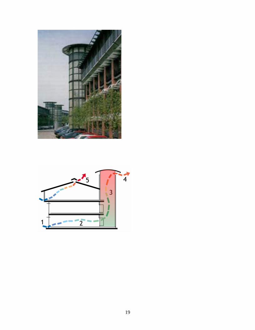
Consider airflow at the ground floor of a building that bears at least passing resemblance to the Inland Revenue building in Nottingham. Determine how warm it can be outside while maintaining comfortable conditions inside. Proceed as follows in CONTAMW:

Set up a model that has three zones: an office zone, a hallway, and a stairwell.

Define an opening across the outer wall of the office, across the wall that separates office and hallway, across the boundary between hall and stairwell, and at the top of the stairwell. For the last, it is acceptable to simply put the opening high in the wall rather than in the roof. Size these using your good sense as designers, or what you may know about the building.

Pick the upper bound of what you feel is an appropriate range of comfortable indoor temperatures. Pick an outdoor temperature that is moderately lower.

Use CONTAMW to calculate the airflow, in m3/h.

As with the auditorium design exercise, calculate the heat flow associated with this airflow.

Estimate how much heat you would need to remove from a single office. Include lights, the occupant(s), office equipment, and perhaps solar energy.

Compare the heat flows. If the simulation shows that you are removing more heat than you need to, bump up the outdoor temperature and try again.

Try a couple of variations in office heat loads. What do you conclude about the need to control solar energy? Try a couple of variations in the temperature of the stairwell, which could correspond to the impact of solar energy. Does a solar chimney make a significant difference?

Try reducing the height between the inlet window in the office and the outlet opening in the stairwell, to a level that corresponds to the second story. How does the maximum outdoor temperature vary, for the same heat loads and opening areas?

18

19

Buoyancy-driven flows in a multi-story building

Finish your exploration of CONTAMW for design of buildings with buoyancy-driven flows by modeling a two-story building with an attached atrium. This requires you to create new floors and to make the atrium two stories in height. Proceed as follows:

Draw a rectangular box and then slice in two vertically to make two zones. Create zone icons and define the zones. Call the left-hand zone “firstfloor.” Call the right-hand zone the atrium and give it a volume and floor area that corresponds to at least two floors. In short, the implicit height should be at least twice that of the occupied ground-floor zone.

Using the level pull-down menu, copy the level, then paste above, to create a second floor.

Click on the zone icon in the second-floor occupied zone and change the name to “secondfloor,” to denote that you are now in the occupied zone on the second level. Click on the zone icon for the second-floor atrium zone and then use the edit command to remove it. Then right-click in this zone to create a phantom zone. By definition, this is connected to the zone below.

Define flow paths. The first floor needs an inlet from ambient and an outlet into the atrium. So does the second floor. The atrium needs an outlet to ambient. If you use the default flow-path heights, your openings will be 1.5 m above the floor reference levels. This is acceptable for all openings except the atrium outlet, which should be higher, above the height of the second-floor windows. Remember that a flow coefficient of 0.77 corresponds to an opening area of 1 m2.

For starters, select the same indoor temperature for all three zones and a cooler temperature for ambient.

Simulate the flows and examine the results. How much lower is the flow through the second floor occupied zone? Try a number of cases. First, note what happens as the height of the atrium outlet is dropped. Do you reach a point where air flows out of the atrium and into the second floor, rather than the in the desired direction? Then try varying opening areas and/or zone temperatures. A warmer atrium would correspond to absorption of solar energy.

20

Contaminant dispersal with CONTAMW 2.0

This section of the notes considers the use of ozone as a tracer to model airflows in a building. The ozone is generated with a corona discharge and is measured with one or more tin-oxide detectors for which the electrical resistance changes with ozone deposition. The general approach is appropriate to analyze the dispersal of any contaminant and the use of any tracer gas.

Constant injection

Model the build-up of a tracer from zero concentration to a steady value in a single-zone space with buoyancy-driven flow.

Model the zone, inlet and outlet as before.

Define a contaminant species, O3. Open the data pull-down menu and select contaminant, then new. Give ozone a molecular weight of 48 (molecular weights are used by CONTAMW to convert volume fractions to mass fractions) and a default concentration of 0, and specify that it will be used in a simulation. Alternatively, if the species tab is selected under the data menu, a contaminant can be imported from a species library.

Right click in the zone to define a source. Then double-click on the source, select a new element, and select constant coefficient. Name the source, then specify a generation rate, say, 0.01 kg/s.

Open the simulation pull-down menu, select simulation parameters, and specify a transient simulation for contaminants. Run the simulation, then plot the contaminant results.

The result shows a rise toward a steady value of about 0.027 kg/kg, for a space volume of 300 m3 and an airflow rate of about 1095 m3/h. Is this reasonable? The airflow rate is about 0.3 m3/s or 0.36 kg/s for a density of 1.2 kg/m3. A concentration of 0.027 kg/kg gives a ozone transport rate of 0.36*0.027=0.0097 kg/s, in agreement with the specified source of 0.01 kg/s.

If the ozone source were known, the measured concentration could be used to determine the airflow rate. However, it is not possible to measure the source strength of the corona discharge. This eliminates the use of ozone under the constant-injection or constant-concentration protocols but allows its use for decay tests.

21

To run a decay test, return to the definition of the source and set the generation rate to zero. Double-click on the zone and set the initial value of the contaminant to 0.01 kg/kg. Change the simulation parameters: under run control, specify a calculation time of one minute (five-minute default) and a display time of five minutes (one-hour default). Under output, change the listing time to five minutes (one-hour default). Run the simulation and plot the contaminant concentration. A time-constant can be determined from the transient plot, which is the inverse of the air-change rate.

Alternatively, set the initial concentration to zero but set the default value to 0.01 kg/kg. Run the simulation. Plot the contaminant and note that it rises to the default value, the inverse of a decay test. The time constant can be determined as noted above.

The burst mode allows a mass of contaminant to be injected according to a schedule. The schedule is for a 12-day week, which includes five days for holidays. The daily schedule can include spikes for bursts. The spikes must be at least as long as the simulation time step. With adequate resolution for output, the expected exponential decay is clearly revealed.

Duct systems

Ducts can be added. The duct tool is used to draw a duct. Clicking on the duct icon allows the duct to be defined. The fittings can also be defined. A duct inserted across the room wall will take a small amount of outflow. If the duct is defined to have a constant flow rate, it can be used to exhaust the room.

There appears to be nothing in the duct definition that accounts for dispersal of contaminants.

22

Decay tests