Are Banks Too Big to Fail? Measuring Systemic Importance ... · Are Banks Too Big to Fail? Measuring Systemic Importance of Financial Institutions∗ Chen Zhou De Nederlandsche Bank

Are Banks Too Big to Fail? MeasuringSystemic Importance of Financial Institutions∗

Chen ZhouDe Nederlandsche Bank and Erasmus University Rotterdam

This paper considers three measures of the systemic impor-tance of a financial institution within an interconnected finan-cial system. The measures are applied to study the relationbetween the size of a financial institution and its systemicimportance. Both the theoretical model and empirical analy-sis reveal that, when analyzing the systemic risk posed by onefinancial institution to the system, size should not be consid-ered as a proxy of systemic importance. In other words, the“too big to fail” argument is not always valid, and measures ofsystemic importance should be considered. We provide the esti-mation methodology of systemic importance measures underthe multivariate extreme value theory (EVT) framework.

JEL Codes: G21, C14.

1. Introduction

During financial crises, authorities have an incentive to prevent thefailure of a financial institution because such a failure would posea significant risk to the financial system, and consequently to thebroader economy. A bailout is usually supported by the argumentthat a financial firm is “too big to fail”: that is, larger banks exhibithigher systemic importance. A natural question arising from thedebate on bailing out large financial firms is why particularly large

∗The author thanks Markus Brunnermeier, Gabriele Galati, Douglas Gale,Miguel Segoviano, Stefan Straetmans, Casper de Vries, Haibin Zhu, participantsat the second Financial Stability conference of the International Journal of Cen-tral Banking, and an anonymous referee for useful discussion and suggestions.Views expressed do not necessarily reflect official positions of De NederlandscheBank. Author postal address: Economics and Research Division, De Nederland-sche Bank, 1000AB Amsterdam, The Netherlands. E-mail: [email protected].

205

206 International Journal of Central Banking December 2010

banks should be favored: are banks really too big to fail? An equiv-alent question might also be posed: does the size of a bank reallymatter for its systemic impact if it fails? The major difficulty inanswering such a question is to design measures on the systemicimportance of financial institutions. More specifically, we need tomeasure to what extent the failure of a particular bank will “con-tribute” to the systemic risk.

This paper deals with the problem in four steps. Firstly, wediscuss the potential drawbacks of existing measures of systemicimportance and propose alternatives that overcome these drawbacks.Secondly, we construct a theoretical model to assess whether largerbanks correspond with higher systemic importance. Thirdly, weemploy statistical methodology in estimating such measures withina constructed system consisting of twenty-eight U.S. banks. Finally,we use the estimated systemic importance measures and the sizemeasures to empirically test the “too big to fail” statement.

Although the term “too big to fail” appears frequently in sup-port of bailout activities, its downside is well acknowledged in theliterature. Besides the distortion of the market discipline, the pref-erence given to large financial firms encourages excessive risk-takingbehavior, which potentially imposes more risk. Therefore, using the“too big to fail” argument to support intervention will result in amoral hazard problem: large firms that the government is compelledto support were among the greatest risk takers during the boomperiod. Furthermore, such a moral hazard problem will provide anincentive for firms to grow in order to be perceived as “too big tofail” (see Stern and Feldman 2004 for more discussions on the moralhazard problem).

Recently, both policymakers and academicians have begun todistinguish the size of a financial institution from the systemicimportance it has by introducing new terms focusing on what thepotential systemic impact might be if that particular institutionfails. For example, Bernanke (2009) addresses the problem of finan-cial institutions that are deemed “too interconnected to fail”; Rajan(2009) uses the term “too systemic to fail” to set the central focusof new regulation development. This urges the design of alternativemeasures on systemic importance. Measuring the systemic impor-tance of financial institutions is particularly important for policy-makers. It is the key issue in both financial stability assessment

Vol. 6 No. 4 Are Banks Too Big to Fail? 207

and macroprudential supervision. On the one hand, during crises,it is necessary to have such measures in order to justify bailoutactions. On the other hand, it is crucial to supervise and monitorbanks with higher systemic importance during regular periods. Pol-icy proposals for stabilizing the financial system always rely on suchmeasures. For instance, charging a deposit insurance premium is analternative proposed by Acharya, Santos, and Yorulmazer (2010) fordefending systemic risk. Systemic importance measures can serve asan indicator for pricing the corresponding insurance premium ortaxation.

A few applicable measures of systemic importance have appearedin recent empirical studies. Adrian and Brunnermeier (2008) pro-posed the conditional value-at-risk (CoVaR) for measuring riskspillover. Similar to the value-at-risk measure, which quantifies theunconditional tail risk of a financial institution, the CoVaR quan-tifies how the financial stress of one institution can increase thetail risk of others. These measures demonstrate the bilateral rela-tion between the tail risks of two financial institutions. The setupof the CoVaR measure indicates that it is designed for bilateral riskspillover. When applying CoVaR to assess the systemic importanceof one financial institution to the system, it is necessary to constructa system indicator on the status of the system and then to analyzethe bilateral relation between the system indicator and a specificbank. However, the complexity of the financial system is of a higherorder than bilateral relations. Thus, a general indicator of the systemis usually difficult to construct. Furthermore, the CoVaR measure isdifficult to generalize into a systemic context in order to analyze mul-tiple financial institutions all together. As an alternative, Segovianoand Goodhart (2009) introduced the “probability that at least onebank becomes distressed” (PAO). Comparing these two measures,we observe that the CoVaR is a measure of conditional quantile,while the PAO is a measure of conditional probability, which acts asthe counterpart of conditional quantile. Within a probability setup,generalization from bivariate to multivariate is possible. However,the PAO measure focuses on the probability of having a systemicimpact that there will be at least one extra crisis, without spec-ifying how severe the systemic impact is. Therefore, the measuremay not provide sufficient information on the systemic importanceof a financial institution. Our empirical results partially reflect the


less informative feature of the PAO: the PAO measures remain at aconstant level across different financial institutions and across time.

Extending the PAO measure while staying within the multivari-ate context, we propose the systemic impact index (SII), which meas-ures the expected number of bank failures in the banking systemgiven a situation in which one particular bank fails. Clearly, the SIImeasure emphasizes more the systemic impact. We also consider areversed measure: the probability that a particular bank fails, giventhat there exists at least one other failure in the system. This werefer to as the vulnerability index (VI).

To test “too big to fail,” we first consider a theoretical modelfrom which both size and systemic importance measures can beexplicitly calculated. The model stems from the literature on sys-temic risk. In the literature, two categories of models consider crisiscontagion and systemic risk in the banking system: banks are sys-temically linked via either direct channels such as interbank marketsor indirect channels such as similar portfolio holdings in bank bal-ance sheets. Studies in the first category focus on the contagioneffect; i.e., a crisis in one financial institution may cause crises in theothers. The second category of studies focuses on modeling systemicrisk; i.e., crises of different financial institutions may occur simulta-neously. For the first category of studies, particularly on modelingthe interbank market, see Allen and Gale (2000), Freixas, Parigi,and Rochet (2000), and Dasgupta (2004). Cifuentes, Shin, and Fer-rucci (2005) consider two channels: similar portfolio holdings andmutual credit exposure. They show that contagion is mainly drivenby changes in asset prices. Hence the indirect channel dominates.For models focusing on the indirect channel, Lagunoff and Schreft(2001) assume that the return of one bank’s portfolio depends onthe portfolio allocation of other banks, and they show that crisescan either spread from one bank to another or happen simultane-ously due to forward-looking behavior. De Vries (2005) starts fromthe fat-tail property of the underlying assets shared by banks, andhe argues that this creates the potential for systemic breakdown.For an overview of contagion and systemic risk modeling, we referto de Bandt and Hartmann (2001) and Allen, Carletti, and Babus(2009).

The contagion literature focuses mainly on explaining the exis-tence of a contagion effect: how a crisis in one financial institution


leads to a crisis in another. Thus, the models usually consider therisk spillover between only two banks. To address the financial sys-tem as a complex entity, several studies have considered networkmodels combined with bilateral spillover. Following those theoret-ical studies, empirical analyses, such as the CoVaR measure, werethen designed for measuring bilateral relations. In order to addressthe systemic importance issue within a systemic context, we mustconsider a multibank approach. Thus, we establish our theoreticalmodel based on the indirect channel models: similar portfolio hold-ings lead to the possibility of simultaneous crises. The fundamentalintuition is that banks are interconnected due to the common expo-sures on their balance sheets. Thus, the systemic importance of aparticular bank is closely associated with the number of differentrisky banking activities in which the bank participates. This, in turn,may not be directly associated with the bank’s size. In other words,“too big to fail” is not always valid. Our model further shows thatbanks concentrating on few specific activities can grow large withoutincreasing their systemic importance.

We acknowledge a potential downside of considering the indi-rect channel model: it does not provide a model on the causalityeffect. Nevertheless, even without addressing the contagion effect,investigating systemic importance based on the systemic risk of hav-ing simultaneous crises is an important issue. This comes from the“too many to fail” phenomenon discussed by Acharya and Yorul-mazer (2007). They consider a game theory approach and show thatbecause regulators would bail out a bank in distress only if a largepart of the system suffers from distresses, individual banks wouldhave an incentive to hold similar portfolios in order to increase thepossibility of being rescued when a crisis occurs. Such a “too manyto fail” phenomenon is in line with the intuition that when evalu-ating systemic importance of a financial institution, it is necessaryto evaluate to what extent the crisis of the financial institution isaccompanied by crises of others. Therefore, we choose to build thesystemic importance measure on an indirect channel model.

The theoretical finding that “too big to fail” is not always validcontributes to policy discussions on micro-level risk management andmacro-level banking supervision. Since diversification is the usualtool in micro-level risk control, financial institutions, particularlythe large ones, tend to take part in more banking activities in order


to diversify away their individual risk. This may, however, increasetheir systemic importance. It is important to acknowledge the trade-off between managing individual risk and maintaining independencewithin the entire banking system. Portfolio construction towardreduction in individual risk may imply a transfer of risk to systemiclinkage and thus increase the systemic importance. Therefore, pru-dential regulations which limit individual risk taking, such as BaselI and II type regulations, are not sufficient for maintaining stabilityof the entire financial system. Macroprudential supervision whichconsiders the system as a whole is necessary for achieving financialstability. A macroprudential approach requires careful considerationof both individual risk taking and the systemic importance of eachindividual financial institution.

Next, we demonstrate how to empirically estimate the proposedsystemic importance measures. We adopt the multivariate extremevalue theory (EVT) framework for empirical estimation. In anyinvestigation of crises, or rare events, the major difficulty is thescarcity of observations on crisis events. Since our intention is toaddress the interconnectedness of the banking crises, which is ineffect a joint crisis, the difficulty with regard to the shortfall inobservations is further enhanced. A modern statistical instrument—EVT—fills the gap. The essential idea of EVT is to model theintermediate-level observations, which are close to extreme, andextrapolate the observed properties into an extreme level. Therefore,the interconnectedness of crises can be approximated by the inter-connectedness of tail events, which are not necessarily at a crisislevel. Univariate EVT has been applied in value-at-risk assessmentfor individual risks (see, e.g., Embrechts, Kluppelberg, and Mikosch1997). Recent developments on multivariate EVT provide the oppor-tunity to investigate extreme co-movements, which serves our pur-pose. For instance, EVT was applied to measure risk contagionsacross different financial markets in Hartmann, Straetmans, and deVries (2004) and Poon, Rockinger, and Tawn (2004). An applicationof multivariate EVT in analyzing bilateral relations within the bank-ing system can be found in Hartmann, Straetmans, and de Vries(2005). Beyond bivariate relations, the Global Financial StabilityReport published by the International Monetary Fund in April 2009(IMF 2009) demonstrates—using EVT analysis—the interconnec-tion of financial distress within a system consisting of three banks.


Our empirical estimation of the systemic importance measures usesmultivariate EVT without restricting the number of banks underconsideration.

We provide an empirical methodology with which to estimatethe systemic importance measures—PAO, SII, and VI—under themultivariate EVT framework. We conduct an exercise for a con-structed system consisting of twenty-eight U.S. banks and test thecorrelation between the systemic importance measures and differ-ent measures on size. We find that, in general, systemic importancemeasures are not correlated with all bank size measures. Hence, thesize of a financial institution should not be considered as a proxyof its systemic importance without careful justification. This agreeswith our theoretical model. Overall, we conclude that it is neces-sary to have proper systemic importance measures for identifyingthe systemically important financial institutions.

2. Systemic Importance Measures

We consider a banking system containing d banks with their statusindicated by (X1, . . . , Xd), where an extremely high value of Xi indi-cates a distress situation or a crisis in bank i. Potential candidatesfor such an indicator might include the loss of equity returns, lossreturns on total asset, or credit default swap (CDS) rates.

To define a crisis, it is necessary to consider what constitutes aproperly high threshold. Our approach takes value-at-risk as such athreshold. For the distress status X of a financial institution, a VaRat a tail probability level p is defined by

P (X > V aR(p)) = p.

Prudential regulations consider the p-level as 1 percent or 0.1 percentin order to evaluate risk-taking behavior of an individual institution.We say that a bank is in crisis if X > V aR(p) with an extremely lowp. Here, we do not specify the level p explicitly. Instead, we imposea restriction that the p-level in the definition of banking crises isconstant across all banks. Notice that banks may differ in their riskprofiles, which results in different endurability on risk, i.e., differentV aR(p). Thus, a unified level of loss for crisis definition may not fitthe diversified situation of different financial institutions. Instead,


an extreme event X > V aR(p) corresponds to a return frequencyas 1/p. Fixing such a frequency for crisis definition takes account ofthe diversity of bank risk profiles. Furthermore, such a definition isaligned with the usual crisis description: for example, with yearlydata, a p equal to 1/50 corresponds to “a crisis once per fifty years.”

The systemic importance measures consider the impact on otherfinancial institutions when one of them falls into crisis. We start fromthe measure proposed by Segoviano and Goodhart (2009): the con-ditional probability of having at least one extra bank failure, giventhat a particular bank fails (PAO). In our model, this measure is thefollowing probability:

PAOi(p) := P ({∃j �= i, s.t. Xj > V aRj(p)}|Xi > V aRi(p)). (1)

We argue that the PAO measure may not provide sufficient infor-mation for identifying the systemically important banks. Considerthe following example. Suppose we have a banking system withbanks categorized into two separate groups. Banks within each groupare strongly linked, while banks from the two groups are indepen-dent of each other. One group contains only two banks, X1 and X2,while the other group contains more banks, X3, . . . , Xd, d > 4. Inother words, X1 and X2 are highly related; X3, . . . , Xd are highlyrelated; and Xi and Xj are independent for any 1 ≤ i ≤ 2 and3 ≤ j ≤ d.

Then the PAO measure for X1, PAO1, will be close to 1 sincea crisis of X1 will be accompanied by a crisis of X2. However, thePAO measure for X3, PAO3, will also be close to 1 because of similarreasoning. When d is high, it is clear that X3 is more systemicallyimportant than X1 because it is associated with a larger fraction ofthe entire banking system. However, this will not be reflected by thecomparison between PAO1 and PAO3. In this example, PAO1 andPAO3 should be at a high, comparable level.

Generally speaking, the PAO measure only provides the prob-ability of a systemic impact when one particular bank fails—thatis, an extra crisis occurring in other financial institutions. It doesnot specify the size of such an impact—that is, the number of extracrises in the entire system. Hence, if every institution in the systemis connected to a certain fraction of the system, the PAO measures


of all should stay at a high, comparable level. With indistinguish-able PAO measures, it is not sufficient to identify the systemicallyimportant financial institutions.

A natural extension of the PAO measure is to consider theexpected number of failures in the system, given that a particu-lar bank fails. This is defined as our systemic impact index (SII).Using the notation above, it can be written as

SIIi(p) := E

⎛⎝ d∑

j=1

1Xj>V aRj(p)|Xi > V aRi(p)

⎞⎠ , (2)

where 1A is the indicator function that is equal to 1 when A holds,and is 0 otherwise.

Since the PAO and SII measures characterize the outlook of thefinancial system when a particular bank fails, a reverse question iswhat the probability of a particular bank failure is when the sys-tem exhibits some distress. To characterize the system distress, weuse the same term as in the PAO measure: there exists at least oneother bank failure. Hence, we define a vulnerability index (VI) byswapping the two items in the PAO definition as follows:

V Ii(p) := P (Xi > V aRi(p)|{∃j �= i, s.t. Xj > V aRj(p)}). (3)

From the definitions, all three measures summarize specific infor-mation on the risk spillover in the banking system. It is necessaryto consider all of them when assessing the systemic importance offinancial institutions.

3. Extreme Value Theory and Systemic ImportanceMeasures

3.1 The Setup of Extreme Value Theory

Consider our d-bank setup. Modeling the crisis of a particular finan-cial institution i corresponds to modeling the tail distribution ofXi. Moreover, modeling the systemic risk—i.e., the extreme co-movements among (X1, . . . , Xd)—corresponds to modeling the taildependence structure of (X1, . . . , Xd). Extreme value theory pro-vides models for such a purpose.


To assess VaR with a low probability level p, univariate EVT canbe applied in modeling the tail behavior of the loss. Since our focusis on systemic risk, we omit the details on univariate risk modeling(see, e.g., Embrechts, Kuppelberg, and Mikosch 1997). MultivariateEVT models consider not only the tail behavior of individual Xi butalso the extreme co-movements among them.

The fundamental setup of multivariate EVT is as follows. Forany x1, x2, . . . , xd > 0, as p → 0, we assume that

P (X1 > V aR1(x1p) or · · · or Xd > V aRd(xdp))p

→ L(x1, x2, . . . , xd), (4)

where V aRi denotes the value-at-risk of Xi, and L is a finite positivefunction.1 The L function characterizes the co-movement of extremeevents that Xi exceeds a high threshold V aRi(xip). (x1, . . . , xd) con-trols the level of high threshold, which in turn controls the directionof extreme co-movement. For the property on the L function, see deHaan and Ferreira (2006).

The value of L at a specific point, L(1, 1, . . . , 1), is a measure ofthe systemic linkage of banking crises among the d banks. From thedefinition in (4), we have

L(1, 1, . . . , 1) = limp→0

P (X1 > V aR1(p) or . . . or Xd > V aRd(p))p

.

(5)

In the context of our banking system, when p is at a low level, itapproximates the quotient ratio between the probability that thereexists at least one bank in crisis and the tail probability p used in thedefinition of individual crisis. For the bivariate case, this was con-sidered by Hartmann, Straetmans, and de Vries (2004) in measuringsystemic risk across different financial markets.

1Notice that considering the union of the events—i.e., using “or” in(4)—is simply a result of the definition of the distribution function. DefineF (x1, . . . , xd) = P (X1 ≤ x1, . . . , Xd ≤ xd) as the distribution function of(X1, . . . , Xd). In order to consider the tail property, the assumption is madeon the tail part 1 − F , which is the probability of the union of extreme events asin relation (4).


Note that the L function is connected with the modern instru-ment of dependence modeling—the copula. Denote the joint distri-bution function of (X1, . . . , Xd) as F (x1, . . . , xd) while the marginaldistributions are denoted as Fi(xi) for i = 1, . . . , d. Then there existsa unique distribution function C(x1, . . . , xd) on [0, 1]d, such that

F (x1, . . . , xd) = C(F1(x1), . . . , Fd(xd)),

where all marginal distributions of C are standard uniform distri-butions. C is called the copula. By decomposing F into marginaldistributions and copula, we separate the marginal information fromthe dependence structure summarized in the copula C. Condition (4)is equivalent to the following relation. For any x1, x2, . . . , xd > 0, asp → 0,

1 − C(1 − px1, . . . , 1 − pxd)p

→ L(x1, x2, . . . , xd).

Hence the L function characterizes the limit behavior of the cop-ula C at the corner point (1, . . . , 1) ∈ [0, 1]d. In other words, the Lfunction captures the tail behavior of the copula C.

Linking the L function to the tail behavior of copula yields thetwo following views. Firstly, since it is connected to the copula, the Lfunction does not contain any marginal information. Thus, in mod-eling the linkage of banking crises, the L function is irrelevant to therisk profile of the individual bank. Secondly, in characterizing thetail behavior of a copula, the L function does not contain depen-dence information at a moderate level, as in the copula C. Instead,L only contains tail dependence information. To summarize, the Lfunction contains the minimal amount of required information inmodeling extreme co-movements. Therefore, models on L are flexi-ble to accommodate all potential marginal risk profiles and potentialmoderate-level dependence structures. Compared to Segoviano andGoodhart (2009), who consider the Consistent Information Multi-variate Density Optimizing (CIMDO) approach on estimating thecopula C, since models on the copula C incorporate the intercon-nection of banking systems in regular time, estimating a copulamodel may misspecify the tail dependence structure. Because weintend to model the interconnection of banking crises, considering


the L function in the multivariate EVT approach is sufficient andless restrictive.

3.2 Systemic Importance Measures under Multivariate EVT

Under the multivariate EVT setup, the limit of the three systemicimportance measures can be directly calculated from the L function.Notice that in the definitions of these measures, the probability levelp for defining crisis is considered. However, we prove that, as p → 0,the systemic importance measures can be well approximated by theirlimits.

The following proposition shows the limit of the PAO measure.The proof is in appendix 1.

Proposition 1. Suppose (X1, X2, . . . Xd) follows the multivariateEVT setup. With the definition of PAO in (1), we have

PAOi := limp→0

PAOi(p) = L�=i(1, 1, . . . , 1) + 1 − L(1, 1, . . . , 1), (6)

where L is the L function characterizing the tail dependence of(X1, . . . , Xd), and L�=i(1, 1, . . . , 1) is the L function characterizingthe tail dependence of (X1, . . . , Xi−1, Xi+1, . . . Xd).

Notice that L is defined on Rd, while L�=i is defined on R

d−1. More-over,

L�=i(1, 1, . . . , 1) = L(1, 1, . . . , 1, 0, 1, . . . , 1),

where 0 appears at the i -th dimension.Proposition 1 shows that when considering a low-level p, the

measure PAOi(p) is close to its limit denoted by PAOi. For calcu-lating PAOi, it is sufficient if the L function is known. Therefore,we could have a proxy of the PAO measure with low-level p by esti-mating the L function. In a theoretical model, the L function can beexplicitly calculated. For an empirical analysis, the L function canbe estimated from historical data. We provide a practical guide forestimating the L function in appendix 2. For more discussions, seede Haan and Ferreira (2006).

Analogous to that of PAO, the limit of VI(p) exists under themultivariate EVT setup. We present the result in the followingproposition but omit the proof.


Proposition 2. Suppose (X1, X2, . . . Xd) follows the multivariateEVT setup. With the definition of VI in (3), we have

VIi := limp→0

VIi(p) =L�=i(1, 1, . . . , 1) + 1 − L(1, 1, . . . , 1)

L�=i(1, 1, . . . , 1), (7)

with the same notation defined in proposition 1.

From propositions 1 and 2, we get the following corollary.

Corollary 1. PAOi > PAOj holds if and only if VIi > VIj.

Corollary 1 implies that when considering the ranking instead of theabsolute level, the VI measure is in fact as informative as the PAOmeasure.

The following proposition shows how to calculate the limit of SIIunder the multivariate EVT setup. The proof appears in appendix 1.

Proposition 3. Suppose (X1, X2, . . . Xd) follows the multivariateEVT setup. With the definition of SII in (2), we have

SIIi := limp→0

SIIi(p) =d∑

j=1

(2 − Li,j(1, 1)), (8)

where Li,j is the L function characterizing the tail dependence of(Xi, Xj).

Notice that

Li,j(1, 1) = L(0, . . . , 0, 1, 0, . . . , 0, 1, 0, . . . , 0),

where 1 appears only at the i -th and j -th dimensions. We remarkthat 2 − Li,j(1, 1) is in fact a measure of bilateral relation betweenthe crises of banks Xi and Xj . Thus, the SII measure is an aggrega-tion of measures on bilateral relations. This is parallel to the spilloverindex studied in Diebold and Yilmaz (2009) when measuring volatil-ity spillover in a multivariate system: after measuring the volatilityspillover between each pair, the spillover index is an aggregation ofthe measures on bilateral relations.


Again, proposition 3 shows that SIIi is a good approximation ofSIIi(p) when p is at a low level. And the estimation of SIIi is onlybased on the estimation of the L function. From the calculation ofPAO and SII, it is clear that the two measures provide differentinformation on systemic importance. A ranking based on PAO doesnot necessarily imply the same ranking on SII. Thus, it is still nec-essary to look at both of the measures in order to obtain a completepicture on the systemic importance of a bank.

To summarize, the multivariate EVT setup provides the oppor-tunity to evaluate all three systemic importance measures when theL function is known. Since the L function characterizes the taildependence structure in (X1, . . . , Xd), all the systemic importancemeasures can be viewed as characterizations of the tail dependenceamong banking crises.

4. Are Banks “Too Big to Fail”? A Theoretical Model

We construct a simple model showing that large banks might havea lower level of systemic importance compared with small banks:banks are not necessarily too big to fail.

We start by reviewing a simple model in de Vries (2005), whichexplains the systemic risk within a two-bank system.

Consider two banks (X1, X2) holding exposures on two indepen-dent projects (Y1, Y2), as in the following affine portfolio model:

{X1 = (1 − γ)Y1 + γY2,X2 = γY1 + (1 − γ)Y2,

(9)

where 0 < γ < 1, (Y1, Y2) indicates the loss returns of the twoprojects. To measure the systemic risk, de Vries (2005) considersthe following measure:

lims→∞

E(κ|κ ≥ 1) := lims→∞

P (X1 > s) + P (X2 > s)P (X1 > s or X2 > s)

. (10)

Intuitively, E(κ|κ ≥ 1) is the expected number of bank crises in thetwo-bank system, given that at least one bank is in crisis. Here, thecrisis of Xi is defined as Xi > s. It is proved that when Yi, i = 1, 2are normally distributed, lims→∞ E(κ|κ ≥ 1) = 1. Thus, given thatthere exists at least one bank in crisis, the expected total number


of crises is 1. Hence, there is no extra crisis except the existing one.This is called a weak fragility case. In other words, the systemicimpact does not exist. To the contrary, suppose Yi, i = 1, 2 followa heavy-tailed distribution on the right tail. The result differs. Theheavy-tailed distribution is defined as

{P (Yi > s) = s−αK(s), i = 1, 2,

P (Yi < −s) = o(P (Yi > s)), (11)

where α > 0 is called the tail index and K(s) is a slowly varyingfunction satisfying

limt→∞

K(ts)K(s)

= 1,

for all s > 0. De Vries (2005) proved that for γ ∈ [1/2, 1],

lims→∞

E(κ|κ ≥ 1) = 1 + (1/γ − 1)α > 1.

This is called the strong fragility case because one existing crisiswill be accompanied by potential extra crises. The empirical liter-ature has extensively documented that the losses of asset returnsfollow heavy-tailed distributions. Therefore, the latter model basedon heavy-tailed distributions reflects the empirical observations andexplains the systemic risk existing in the financial system.

We remark that when assuming the heavy-tailedness of (Y1, Y2),and the affine portfolio model in (9), it is a direct consequence that(X1, X2) follows a two-dimensional EVT setup.2 Moreover, if Y1 andY2 are identically distributed, for a fixed tail probability p, the VaRsof X1 and X2 are equal; i.e., V aR1(p) = V aR2(p). Replacing s withV aRi(p) in the definition of the systemic risk measure (10), andasking p → 0, we get

limp→0

E(κ|κ ≥ 1) := limp→0

P (X1 > V aR1(p)) + P (X2 > V aR2(p))P (X1 > V aR1(p) or X2 > V aR2(p))

=2

L(1, 1).

2For a formal proof, see Zhou (2008, ch. 5).


Therefore, the setup in de Vries (2005) imposes a multivariate EVTsetup, and the measure on the systemic risk is essentially based onL(1, 1).

We point out that within this two-bank, two-project model, itis not possible to differentiate the systemic importance of the twobanks. From the model and from proposition 1, we get

SIIi = 3 − L(1, 1), i = 1, 2.

Hence the two banks have equal systemic importance measured bySII. Similar results hold for the other two measures, PAO and VI.Intuitively, within a two-bank setup, the linkage of crises is a mutualbilateral relation. Hence, one could not distinguish the systemicimportance of the two banks. In order to construct a model in whichit is possible to compare the systemic importance at different levels,it would be necessary to generalize the de Vries (2005) model to asystem consisting of at least three banks.

Next, we consider the size issue. In the de Vries (2005) two-bankmodel, suppose that both of the two banks have total capital 1, andboth of the two projects receive capital 1. According to the affineportfolio model (9), the capital market is clear. In this case, the twobanks have the same size in terms of total assets. In order to differ-entiate the sizes of the banks, a more complex affine portfolio modelis necessary.

Addressing the two above-mentioned points, we consider a modelwith three banks (X1, X2, X3) and three independent projects(Y1, Y2, Y3). Suppose X1 holds capital 2 for investment, while X2 andX3 hold capital 1 each. Moreover, suppose the project Y1 demandsan investment 2, while Y2 and Y3 each have a capital demand 1.Then the market is clear, with the following affine portfolio model:

⎧⎨⎩

X1 = (2 − 2γ)Y1 + γY2 + γY3X2 = γY1 + (1 − γ − μ)Y2 + μY3,X3 = γY1 + μY2 + (1 − γ − μ)Y3,

(12)

where 0 < γ, μ < 1, and γ + μ < 1. Clearly, this is not the only pos-sible allocation for market clearance. Nevertheless, it is sufficient todemonstrate our argument regarding the “too big to fail” problem.Notice that X1 is a larger bank compared with X2 and X3. Here, the


size refers to the total investment in the risky projects. We intendto compare the systemic importance of X1 with that of X2 and X3.

The two parameters γ and μ are interpreted as the control ofsimilarity in portfolio holdings across the three banks. The parame-ter γ controls the similarity between the large bank and the smallbanks. When γ is close to 1, the strategy of the large bank is differ-ent from that of the two small banks, while the two small banks holdsimilar portfolios. When γ = 1/2, the large bank has exposures onall three projects proportional to their capital demands. Hence, thelarge bank is involved in all projects. When γ is close to 0, the largebank is again different from the two small banks. In the latest case,the similarity of the two small banks is further controlled by theparameter μ: a μ lying in the middle of (0, 1−γ) shows that the twosmall banks are similar in portfolio holding, while a μ lying closeto the two corners of (0, 1 − γ) corresponds to different strategiesbetween the two small banks.

Suppose all Yi follow a heavy-tailed distribution defined in (11)for i = 1, 2, 3. Then, similar to the two-bank case, (X1, X2, X3) fol-lows a three-dimensional EVT setup. Instead of discussing all pos-sible values on the parameters (γ, μ), we focus on three cases: γ isclose to 1, γ = 1/2, and γ is close to 0. The results from comparingthe SII measures are in the following theorem. The proof is again inappendix 1.

Theorem 1. Consider a three-bank, three-project model with theaffine portfolio given in (12). Suppose the losses of the three projectsexhibit the same heavy-tailed feature as in (11), with α > 1. We havethe following relations.

Case 1: 23 ≤ γ < 1

SSI1 < 1 = SSI2 = SSI3.

Case 2: γ = 12

SSI1 ≥ SSI2 = SSI3.

The equality holds if and only if μ = 1/4.

Case 3: 0 < γ < 13


There exists a μ∗ < 1−γ2 such that for any μ satisfying μ∗ < μ <

1 − γ − μ∗,

SSI1 < SSI2 = SSI3.

On the other hand, for any μ satisfying 0 < μ < μ∗ or 1 − γ − μ∗ <μ < 1 − γ, we have

SSI1 > SSI2 = SSI3.

When μ = μ∗ or μ = 1 − γ − μ∗,

SII1 = SII2 = SII3.

The following lemma shows that the comparison among the PAOmeasures follows the comparison among the SII measures in thethree-bank model.

Lemma 1. With the assumptions in theorem 1, the order of PAOfollows the order of SII; i.e., for any i �= j, PAOi > PAOj holds ifand only if SIIi > SIIj.

Combining lemma 1 and corollary 1, we see that the order of VI alsofollows the order of SII in the simple three-bank model. Notice thatthe three-bank model is a very specific and simple case. The resultin lemma 1 does not hold in a general context when the numberof banks is more than three. Therefore, for empirical study within amultibank system, it is still necessary to estimate all three measures,which may provide different views.

We interpret the results in theorem 1 as follows.If γ is close to 1, the large bank X1 focuses on the two smaller

projects Y2 and Y3, while small banks X2 and X3 focus on the largeproject Y1. In this case, the balance sheet of the large bank is quitedifferent from that of the small banks, while the two small banksare holding similar portfolios. Therefore, the large bank has less sys-temic linkage to the other two small banks. We observe that thelarge bank is less systemically important compared with the others;i.e., the large bank is not “too big to fail.”

If γ = 1/2, the large bank X1 invests (1, 1/2, 1/2) in threeprojects. Hence it is involved in all three projects, which creates


the linkage to the other two small banks. In this case, it is “too bigto fail.” The inequality becomes an equation if and only if μ = 1/4.For μ = 1/4, the three banks all invest in three projects proportionalto their capital demands. They have exactly the same strategy inmanaging their portfolios. A crisis in any of the three banks will beaccompanied by crises in the other two. Therefore, they are equallysystemically important. Excluding μ = 1/4, the large bank will bethe most systemically important bank.

If γ is close to 0, the large bank X1 focuses on the large projectY1, while it still has exposures on Y2 and Y3. The small banks X2 andX3 focus on the two small projects Y2 and Y3. Now it matters howsimilar their portfolios are. If μ is in the middle (μ∗ < μ < 1−γ−μ∗),then the balance sheet composition of two small banks is relativelysimilar. Hence, they are more systemically important comparedwith the large bank. If μ is close to the corner (0 < μ < μ∗ or1 − γ − μ∗ < μ < 1 − γ), then the two small banks differ in theirbalance sheets. Since the large bank still has exposures on Y2 andY3 equally, it is the most systemically important bank. It is worthmentioning that the systemic importance of bank X1 is determinednot only by its own risk positions but also by the risk-taking behav-ior of the others. Even though the portfolio of bank X1 is fixed byfixing γ, the change of the portfolios hold by the other two bankscan still result in a change of the systemic importance of X1.

To summarize, we observe that “too big” is not necessarily thereason for being “too systemically important.” Instead, a bank hav-ing a balance sheet that is exposed to more risky projects wouldcause it to become more systemically important. Here, we regardYi, i = 1, 2, 3 as different risky projects. One may also regard themas different risky banking activities. Therefore, a bank that is morediversified in banking activities may turn out to be “too big to fail.”

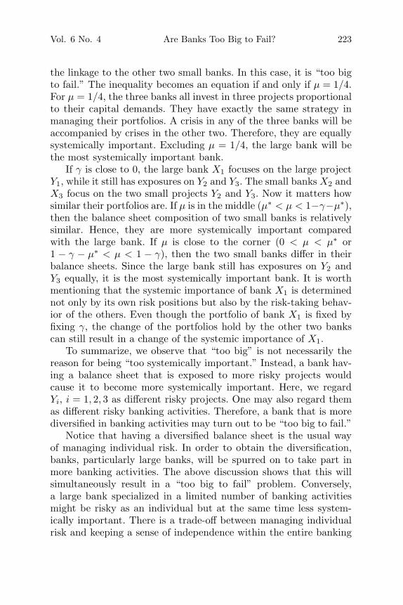
Notice that having a diversified balance sheet is the usual wayof managing individual risk. In order to obtain the diversification,banks, particularly large banks, will be spurred on to take part inmore banking activities. The above discussion shows that this willsimultaneously result in a “too big to fail” problem. Conversely,a large bank specialized in a limited number of banking activitiesmight be risky as an individual but at the same time less system-ically important. There is a trade-off between managing individualrisk and keeping a sense of independence within the entire banking


system. For maintaining the stability of the financial system, it isnecessary for the regulators to recognize such a trade-off and imposeproper regulations in order to give banks incentives to balance theirindividual risk position and systemic importance.

5. Empirical Results

5.1 Empirical Setup and Data

We apply the three proposed measures of systemic importance to anartificially constructed financial system consisting of twenty-eightU.S. banks. After estimating the three measures, we calculate thecorrelation coefficients between these measures and the measures ofthe size of the banks. From the test on correlation coefficients, we canempirically test whether larger banks exhibit larger systemic impor-tance, thereby testing the “too big to fail” argument. We also con-sider a moving window approach, which demonstrates the variationof the systemic importance measures across time.

The data set for constructing the systemic importance meas-ures consists of daily equity returns of twenty-eight U.S. bankslisted on the New York Stock Exchange (NYSE) from 1987 to 2009(twenty-three years).3 The chosen banks are listed in table 1 withthe descriptive statistics on their stock returns.

Regarding the size of the banks, the data set consists of variousmeasures. We consider total assets, total equity, and total debt forthe twenty-eight banks.4 The data that appear are reported in ayearly frequency from 1987 to 2009. For each bank, we present theend-of-2009 values as well as the average values across the twenty-three years in table 2.

From the descriptive statistics of the equity returns, we observethat all daily returns exhibit high kurtosis compared with the

3The data are obtained from Datastream. Three selection criteria are applied:the financial institutions should be classified in the sector “Banks”; they shouldbe traded primarily on the NYSE (DS code starting with “U:”); and the timeseries should be active from the beginning of 1987 till the end of 2009. Theselection procedure results in twenty-eight banks.

4The data on total assets, total equity, and total debt are obtained from Data-stream, with item code WC02999, WC03501, and WC03255, respectively. Noticethat total debt consists of short-term debt, current portion of long-term debt,and long-term debt.


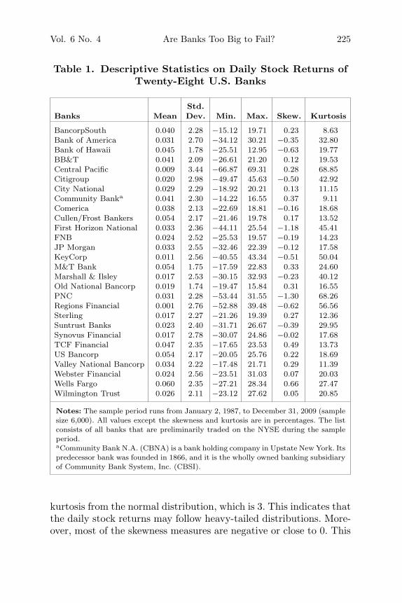
Table 1. Descriptive Statistics on Daily Stock Returns ofTwenty-Eight U.S. Banks

Std.Banks Mean Dev. Min. Max. Skew. Kurtosis

BancorpSouth 0.040 2.28 −15.12 19.71 0.23 8.63Bank of America 0.031 2.70 −34.12 30.21 −0.35 32.80Bank of Hawaii 0.045 1.78 −25.51 12.95 −0.63 19.77BB&T 0.041 2.09 −26.61 21.20 0.12 19.53Central Pacific 0.009 3.44 −66.87 69.31 0.28 68.85Citigroup 0.020 2.98 −49.47 45.63 −0.50 42.92City National 0.029 2.29 −18.92 20.21 0.13 11.15Community Banka 0.041 2.30 −14.22 16.55 0.37 9.11Comerica 0.038 2.13 −22.69 18.81 −0.16 18.68Cullen/Frost Bankers 0.054 2.17 −21.46 19.78 0.17 13.52First Horizon National 0.033 2.36 −44.11 25.54 −1.18 45.41FNB 0.024 2.52 −25.53 19.57 −0.19 14.23JP Morgan 0.033 2.55 −32.46 22.39 −0.12 17.58KeyCorp 0.011 2.56 −40.55 43.34 −0.51 50.04M&T Bank 0.054 1.75 −17.59 22.83 0.33 24.60Marshall & Ilsley 0.017 2.53 −30.15 32.93 −0.23 40.12Old National Bancorp 0.019 1.74 −19.47 15.84 0.31 16.55PNC 0.031 2.28 −53.44 31.55 −1.30 68.26Regions Financial 0.001 2.76 −52.88 39.48 −0.62 56.56Sterling 0.017 2.27 −21.26 19.39 0.27 12.36Suntrust Banks 0.023 2.40 −31.71 26.67 −0.39 29.95Synovus Financial 0.017 2.78 −30.07 24.86 −0.02 17.68TCF Financial 0.047 2.35 −17.65 23.53 0.49 13.73US Bancorp 0.054 2.17 −20.05 25.76 0.22 18.69Valley National Bancorp 0.034 2.22 −17.48 21.71 0.29 11.39Webster Financial 0.024 2.56 −23.51 31.03 0.07 20.03Wells Fargo 0.060 2.35 −27.21 28.34 0.66 27.47Wilmington Trust 0.026 2.11 −23.12 27.62 0.05 20.85

Notes: The sample period runs from January 2, 1987, to December 31, 2009 (samplesize 6,000). All values except the skewness and kurtosis are in percentages. The listconsists of all banks that are preliminarily traded on the NYSE during the sampleperiod.aCommunity Bank N.A. (CBNA) is a bank holding company in Upstate New York. Itspredecessor bank was founded in 1866, and it is the wholly owned banking subsidiaryof Community Bank System, Inc. (CBSI).

kurtosis from the normal distribution, which is 3. This indicates thatthe daily stock returns may follow heavy-tailed distributions. More-over, most of the skewness measures are negative or close to 0. This


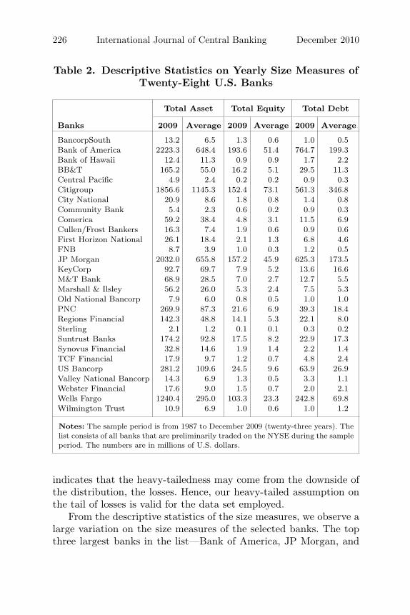
Table 2. Descriptive Statistics on Yearly Size Measures ofTwenty-Eight U.S. Banks

Total Asset Total Equity Total Debt

Banks 2009 Average 2009 Average 2009 Average

BancorpSouth 13.2 6.5 1.3 0.6 1.0 0.5Bank of America 2223.3 648.4 193.6 51.4 764.7 199.3Bank of Hawaii 12.4 11.3 0.9 0.9 1.7 2.2BB&T 165.2 55.0 16.2 5.1 29.5 11.3Central Pacific 4.9 2.4 0.2 0.2 0.9 0.3Citigroup 1856.6 1145.3 152.4 73.1 561.3 346.8City National 20.9 8.6 1.8 0.8 1.4 0.8Community Bank 5.4 2.3 0.6 0.2 0.9 0.3Comerica 59.2 38.4 4.8 3.1 11.5 6.9Cullen/Frost Bankers 16.3 7.4 1.9 0.6 0.9 0.6First Horizon National 26.1 18.4 2.1 1.3 6.8 4.6FNB 8.7 3.9 1.0 0.3 1.2 0.5JP Morgan 2032.0 655.8 157.2 45.9 625.3 173.5KeyCorp 92.7 69.7 7.9 5.2 13.6 16.6M&T Bank 68.9 28.5 7.0 2.7 12.7 5.5Marshall & Ilsley 56.2 26.0 5.3 2.4 7.5 5.3Old National Bancorp 7.9 6.0 0.8 0.5 1.0 1.0PNC 269.9 87.3 21.6 6.9 39.3 18.4Regions Financial 142.3 48.8 14.1 5.3 22.1 8.0Sterling 2.1 1.2 0.1 0.1 0.3 0.2Suntrust Banks 174.2 92.8 17.5 8.2 22.9 17.3Synovus Financial 32.8 14.6 1.9 1.4 2.2 1.4TCF Financial 17.9 9.7 1.2 0.7 4.8 2.4US Bancorp 281.2 109.6 24.5 9.6 63.9 26.9Valley National Bancorp 14.3 6.9 1.3 0.5 3.3 1.1Webster Financial 17.6 9.0 1.5 0.7 2.0 2.1Wells Fargo 1240.4 295.0 103.3 23.3 242.8 69.8Wilmington Trust 10.9 6.9 1.0 0.6 1.0 1.2

Notes: The sample period is from 1987 to December 2009 (twenty-three years). Thelist consists of all banks that are preliminarily traded on the NYSE during the sampleperiod. The numbers are in millions of U.S. dollars.

indicates that the heavy-tailedness may come from the downside ofthe distribution, the losses. Hence, our heavy-tailed assumption onthe tail of losses is valid for the data set employed.

From the descriptive statistics of the size measures, we observe alarge variation on the size measures of the selected banks. The topthree largest banks in the list—Bank of America, JP Morgan, and


Citigroup—are approximately 1,000 times larger than the smallestbank in the list, Sterling Banc, in all aspects. Although the criterionthat the selected banks have to be active in the stock market fortwenty-three years may result in a sample selection bias, since suchbanks are more likely to be large banks, the variation of the sizemeasures shows that the constructed banking system contains bothlarge and small banks.

Using the stock returns is a natural choice for our approach inanalyzing the systemic importance. The restriction imposed by themethodology of estimating the L function is that the sample sizehas to be sufficient; see appendix 2. Moreover, since we intend toperform a moving window analysis, the restriction on the length ofthe time series is further enhanced. Therefore, daily or higher fre-quency is necessary for a full non-parametric approach. This limitsus to using financial market data. Equity returns are the most con-venient choice. Other high-frequency indicators such as CDS spreadsare also possible. Nevertheless, the CDS data do not go back for asufficiently long period, which keeps us from performing a movingwindow analysis. It is also possible to apply the proposed method-ology with low-frequency data, such as return on asset from bankbalance sheet. In that case, a full non-parametric estimate on the Lfunction is not applicable. Instead, further modeling on the L func-tion should be considered. In this study we intend to illustrate themethodology without modeling the L function. Hence, we stick tothe equity return data.

5.2 Estimation of the Systemic Importance Measures

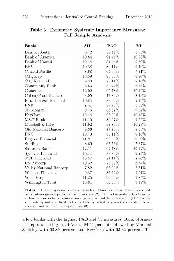
By estimating the L function (for details, see appendix 2), we obtainthe estimates of the three systemic importance measures (SII, PAO,and VI) across the full sample period, as shown in table 3. We startwith the PAO measure proposed by Segoviano and Goodhart (2009).A general observation is that all of the estimates are quite high(above 60 percent). This is in line with our prediction that the PAOmeasures of all banks in a system are at a relatively high level and donot differ much from each other. Since the PAO measure is directlyconnected to the VI measure as shown in corollary 1, a similar featureis observed for the VI measures. In fact, the order of the VI measuresfollows that of the PAO measures as proved in corollary 1. To name


Table 3. Estimated Systemic Importance Measures:Full Sample Analysis

Banks SII PAO VI

BancorpSouth 6.72 59.44% 6.73%Bank of America 10.84 94.44% 10.28%Bank of Hawaii 10.44 84.44% 9.30%BB&T 10.88 86.11% 9.46%Central Pacific 8.68 65.00% 7.31%Citigroup 10.59 90.56% 9.90%City National 9.30 76.11% 8.46%Community Bank 6.53 59.44% 6.73%Comerica 12.02 92.78% 10.12%Cullen/Frost Bankers 8.05 73.89% 8.23%First Horizon National 10.84 83.33% 9.19%FNB 7.41 57.78% 6.55%JP Morgan 9.76 86.67% 9.52%KeyCorp 12.44 93.33% 10.18%M&T Bank 11.10 86.67% 9.52%Marshall & Ilsley 11.92 93.89% 10.23%Old National Bancorp 9.36 77.78% 8.63%PNC 10.73 86.11% 9.46%Regions Financial 11.91 90.56% 9.90%Sterling 8.69 65.56% 7.37%Suntrust Banks 12.11 92.78% 10.12%Synovus Financial 10.11 83.89% 9.24%TCF Financial 10.57 81.11% 8.96%US Bancorp 10.32 78.89% 8.74%Valley National Bancorp 7.82 65.00% 7.31%Webster Financial 9.87 82.22% 9.07%Wells Fargo 11.25 90.00% 9.85%Wilmington Trust 10.91 83.33% 9.19%

Notes: SII is the systemic importance index, defined as the number of expectedbank failures given a particular bank fails; see (2). PAO is the probability of havingat least one extra bank failure when a particular bank fails, defined in (1). VI is thevulnerability index, defined as the probability of failure given there exists at leastanother bank failure in the system; see (3).

a few banks with the highest PAO and VI measures, Bank of Amer-ica reports the highest PAO at 94.44 percent, followed by Marshall& Ilsley with 93.89 percent and KeyCorp with 93.33 percent. The


corresponding VI measures are 10.28 percent, 10.23 percent, and10.18 percent, respectively. At the bottom of the list ranked bythe PAO measure, we have FNB, BancorpSouth, and CommunityBank.5

The SII measure introduced in this paper gives a somewhat dif-ferent outlook compared with the PAO measure. The three lowestSII banks are the same as those with the lowest three PAO measures,although with a different order. The lowest SII measure comes fromCommunity Bank, which is 6.53. This means that if CommunityBank is experiencing a crisis, it will be accompanied by an aver-age of 5.53 extra failures in this system. Compared with the size ofthe system, twenty-eight banks, this is not a high systemic impact.The highest estimated SII measure is 12.44 from KeyCorp, which isalmost twice as high as the lowest value. A crisis of KeyCorp willbe accompanied by an average of 11.44 extra crises in this system,twice the systemic impact of Community Bank. Hence, we observea variation of the SII measure across different banks. To name a fewwith the highest SII measures, the top three are KeyCorp (12.44),Suntrust Banks (12.11), and Comerica (12.02). They are differentfrom the banks with the top-three highest PAO. In general, rank-ing the PAO measures is different from ranking the SII measures.For example, the bank with the highest PAO, Bank of America, isonly ranked at tenth place among all banks when considering theSII measure.

To summarize, the comparison between the three measures showsthat although they have different economic backgrounds, the PAOmeasure and the VI measure are equally informative in terms ofranking the systemic importance of financial institutions. The SIImeasure, in contrast, provides information on the size of the sys-temic impact corresponding to the failure of a particular bank. Ittherefore provides a different view than the other two. Across differ-ent banks, the SII measures vary while the PAO measures remain ata high, comparable level. This agrees with our theoretical prediction.Therefore, the SII measure is more informative in distinguishing thesystemic importance of financial institutions.

5Community Bank N.A. (CBNA) is a bank holding company in Upstate NewYork. Its predecessor bank was founded in 1866, and it is the wholly ownedbanking subsidiary of Community Bank System, Inc. (CBSI).


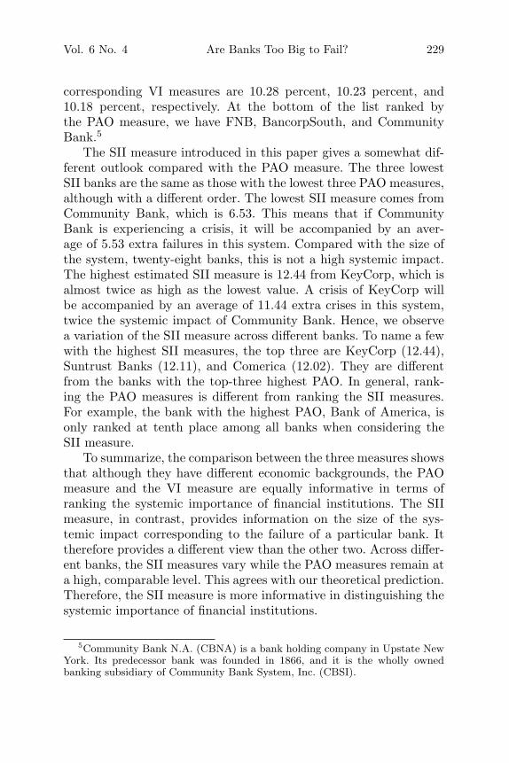
Besides estimating the three systemic importance measures fromthe full sample period, we consider sub-samples for the estimationand perform a moving window approach. By moving the sub-samplewindow, we could obtain time-varying estimation on the systemicimportance measures. We consider the estimation window as 2,000days (approximately eight years), and then move the estimation win-dow forward month by month. The first possible window ends atSeptember 1994. In other words, the first estimation considers dataending at September 30, 1994, and going back 2,000 days. From thenon, we take the end of each month as the ending day of each esti-mation window and use the data going back 2,000 days. By movingthe estimation window month by month, we observe the estimatesat the end of each month from September 1994 to December 2009.For simplicity’s sake, we only plot the results for selected banks,6

as shown in figure 1. The upper panel shows the moving windowSII measures, and the bottom panel shows the moving window PAOmeasures. The two vertical lines in the two figures correspond to thefailures of two large investment banks: Bear Stearns (March 2008)and Lehman Brothers (September 2008).

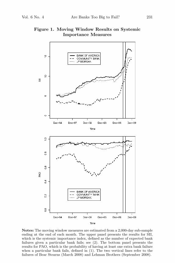
From the moving window SII estimates, we observe that the SIImeasures gradually increased from 1998 to 2003, then remained rel-atively stable until the end of 2006. From 2007, there was a sharprise. The sharp rise of SII started before the failure of Bear Stearnsand continued with the failure of Lehman Brothers, until early 2009.From mid-2009, the SII measures became stable and with a slightdownward slope. In contrast, the PAO measures are stable acrosstime, particularly for the large banks. Only for the least systemi-cally important bank can some variation be observed. This is dueto the fact that the PAO measures of large banks were already at ahigh level in the early period of our sample. It would thus be difficultto obtain a further rise to a higher level.

The observations from the moving window approach again con-firm our theoretical prediction that the PAO measures always stayat a high, comparable level, while the SII measure varies across time

6We select the least systemically important bank, Community Bank, and thetwo largest banks, Bank of America and JP Morgan, in the plots. According tothe full sample analysis, Bank of America is the most systemically importantbank in terms of PAO.


Figure 1. Moving Window Results on SystemicImportance Measures

Notes: The moving window measures are estimated from a 2,000-day sub-sampleending at the end of each month. The upper panel presents the results for SII,which is the systemic importance index, defined as the number of expected bankfailures given a particular bank fails; see (2). The bottom panel presents theresults for PAO, which is the probability of having at least one extra bank failurewhen a particular bank fails, defined in (1). The two vertical lines refer to thefailures of Bear Stearns (March 2008) and Lehman Brothers (September 2008).


and across institutions. The sharp rise of the SII measures addressesthe crisis starting from 2008 and hence is more informative in ana-lyzing the systemic risk in a financial system. Although we observean early rise before the crisis, we do not emphasize that the SIImeasure is a predictor of the crisis. The sharp rise of SII measuresmight either be a predictor of the crisis or an ex post consequencecaused by the crisis. The intuition for the latter possibility is as fol-lows. Banks tend to take similar strategies, such as fire sales, duringa crisis, which may result in more similar portfolio holdings acrossall banks. According to the theoretical model in section 4, that sim-ilarity leads to an increase of the SII measures on all banks. Hence,the timing of the sharp rising of the SII measures is still an openissue for further study.

There are a few other observations from the moving windowanalysis. Notice that the financial system we have constructed con-tains twenty-eight banks. An SII measure of 15 means that if acertain bank fails, there will be an average of fourteen extra bankfailures simultaneously. This is half of the entire system, which mustbe considered as a severe risk. Hence, the observed SII measures fromthe end of 2008 to mid-2009 indicate that the banking system suf-fers severe systemic risk during the crisis. Moreover, it is remarkablethat Community Bank, the least systemically important bank fromthe full sample analysis, also showed the least systemic importanceduring the crisis. Nevertheless, the absolute level of the SII measurereached a comparable level with the other large banks. This sug-gests that size may not be a good proxy of systemic importance,particularly during periods of crisis.

5.3 Test “Too Big to Fail”

We use the estimated systemic importance measures to checkwhether they are correlated with the size measures. The correla-tion test is across different banks; thus, we need to have a unifiedvalue for each individual bank on each size measure. Since the sam-ple period ends in year 2009, we first consider the end-of-2009 valuesof each size measure. The second approach is to take an average ofthe size measures over the full sample period (from 1987 to 2009).Then, we calculate the Pearson correlation coefficients betweeneach pair of size measure and systemic importance measure across


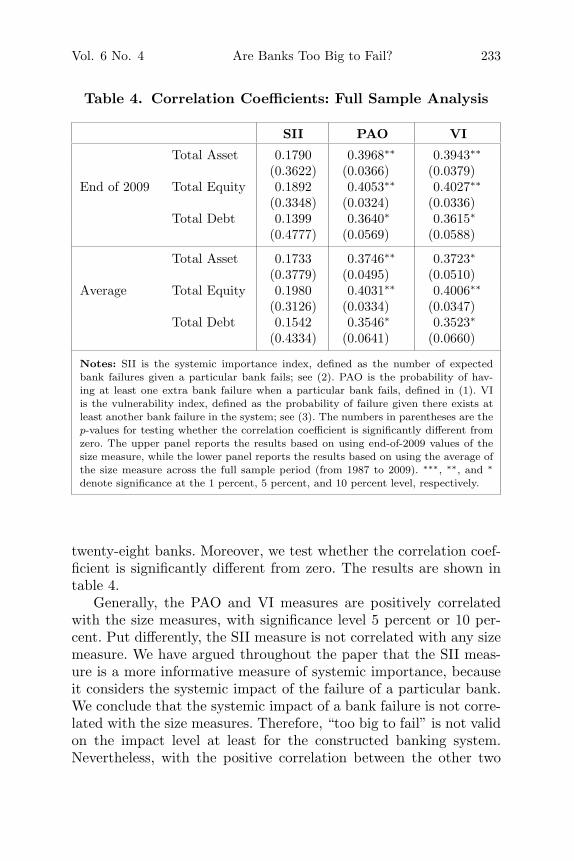
Table 4. Correlation Coefficients: Full Sample Analysis

SII PAO VI

Total Asset 0.1790 0.3968∗∗ 0.3943∗∗

(0.3622) (0.0366) (0.0379)End of 2009 Total Equity 0.1892 0.4053∗∗ 0.4027∗∗

(0.3348) (0.0324) (0.0336)Total Debt 0.1399 0.3640∗ 0.3615∗

(0.4777) (0.0569) (0.0588)

Total Asset 0.1733 0.3746∗∗ 0.3723∗

(0.3779) (0.0495) (0.0510)Average Total Equity 0.1980 0.4031∗∗ 0.4006∗∗

(0.3126) (0.0334) (0.0347)Total Debt 0.1542 0.3546∗ 0.3523∗

(0.4334) (0.0641) (0.0660)

Notes: SII is the systemic importance index, defined as the number of expectedbank failures given a particular bank fails; see (2). PAO is the probability of hav-ing at least one extra bank failure when a particular bank fails, defined in (1). VIis the vulnerability index, defined as the probability of failure given there exists atleast another bank failure in the system; see (3). The numbers in parentheses are thep-values for testing whether the correlation coefficient is significantly different fromzero. The upper panel reports the results based on using end-of-2009 values of thesize measure, while the lower panel reports the results based on using the average ofthe size measure across the full sample period (from 1987 to 2009). ∗∗∗, ∗∗, and ∗

denote significance at the 1 percent, 5 percent, and 10 percent level, respectively.

twenty-eight banks. Moreover, we test whether the correlation coef-ficient is significantly different from zero. The results are shown intable 4.

Generally, the PAO and VI measures are positively correlatedwith the size measures, with significance level 5 percent or 10 per-cent. Put differently, the SII measure is not correlated with any sizemeasure. We have argued throughout the paper that the SII meas-ure is a more informative measure of systemic importance, becauseit considers the systemic impact of the failure of a particular bank.We conclude that the systemic impact of a bank failure is not corre-lated with the size measures. Therefore, “too big to fail” is not validon the impact level at least for the constructed banking system.Nevertheless, with the positive correlation between the other two


systemic importance measures and the size measures, the big banksare more likely to cause extra crises in the system. The bottom lineis that it is not proper to use the size measures as a proxy of sys-temic importance. Instead, it is necessary to consider all of the sys-temic importance measures when identifying systemically importantfinancial institutions.

We have carried out extensive robustness checks for the observedresults. First of all, with the full sample estimation on the systemicrisk measure, we consider the size measure in other years (e.g., endof 2008, 2007, etc.). The results are comparable with those using theend-of-2009 value. We omit the details.

Secondly, instead of the Pearson correlation, we considerthe Spearman correlation, which only emphasizes the correlationbetween ranking orders. The Spearman correlation coefficientsbetween the SII measure and the size measures are significantly dif-ferent from zero. Since the Pearson correlation considers the absolutelevel while the Spearman correlation considers only the rankingorders, we find support of the “too big to fail” argument withinthe constructed system, only in terms of ranking the order.

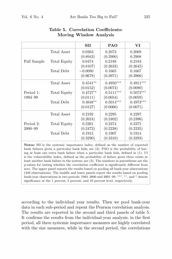
Thirdly, with the moving window results on the systemic impor-tance measures, we can get the end-of-year estimates on the systemicimportance measures from 1994 to 2009 (sixteen years). We pool allof the bank-year estimates together, which results in 28 · 16 = 448estimates for each systemic importance measure, and also 448 obser-vations for each size measure. We then calculate the Pearson correla-tion coefficient for each pair and repeat the test on the significancy.The results appear in the first panel of table 5. None of the threesystemic importance measures are correlated with any of the sizemeasures.

Moreover, since we have obtained sixteen-year data on systemicimportance and size for twenty-eight banks, we also perform thePearson correlation analysis at the level of each year. We observethat the significant positive correlation between size and the PAOmeasure (and the VI measure) is robust for the sub-period 1994–99.From 2000 to 2009, the significance disappears. Interestingly, for thefirst period, the SII measure is also positively correlated with thethree size measures. The (in)significant results are robust withineach sub-period. To further explore these phenomena, we dividethe period 1994–2009 into two sub-periods: 1994–99 and 2000–09,


Table 5. Correlation Coefficients:Moving Window Analysis

SII PAO VI

Total Asset 0.0263 0.2073 0.2069(0.8943) (0.2900) 0.2908

Full Sample Total Equity 0.0474 0.2188 0.2183(0.8107) (0.2633) (0.2645)

Total Debt −0.0080 0.1665 0.1667(0.9678) (0.3971) (0.3966)

Total Asset 0.4541∗∗ 0.4950∗∗∗ 0.4911∗∗∗

(0.0152) (0.0074) (0.0080)Period 1: Total Equity 0.4727∗∗ 0.5111∗∗∗ 0.5072∗∗∗

1994–99 (0.0111) (0.0054) (0.0059)Total Debt 0.4648∗∗ 0.5014∗∗∗ 0.4973∗∗∗

(0.0127) (0.0066) (0.0071)

Total Asset 0.2192 0.2295 0.2297(0.2624) (0.2402) (0.2396)

Period 2: Total Equity 0.2261 0.2374 0.23752000–09 (0.2473) (0.2238) (0.2235)

Total Debt 0.1915 0.1907 0.1914(0.3290) (0.3310) (0.3293)

Notes: SII is the systemic importance index, defined as the number of expectedbank failures given a particular bank fails; see (2). PAO is the probability of hav-ing at least one extra bank failure when a particular bank fails, defined in (1). VIis the vulnerability index, defined as the probability of failure given there exists atleast another bank failure in the system; see (3). The numbers in parentheses are thep-values for testing whether the correlation coefficient is significantly different fromzero. The upper panel reports the results based on pooling all bank-year observations(448 observations). The middle and lower panels report the results based on poolingbank-year observations in two periods: 1994–2000 and 2001–09. ∗∗∗, ∗∗, and ∗ denotesignificance at the 1 percent, 5 percent, and 10 percent level, respectively.

according to the individual year results. Then we pool bank-yeardata in each sub-period and repeat the Pearson correlation analysis.The results are reported in the second and third panels of table 5.It confirms the results from the individual-year analysis: in the firstperiod, all three systemic importance measures are highly correlatedwith the size measures, while in the second period, the correlations


disappear. It suggests that using size as a proxy for systemic impor-tance was proper in the 1990s, but that the situation has changedfrom the beginning of the new century. Therefore, it is particularlyimportant to consider the measures on systemic importance withinthe current financial world.

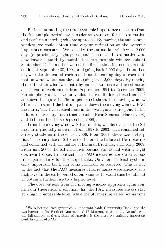
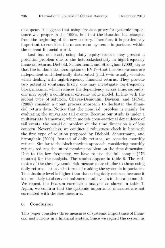
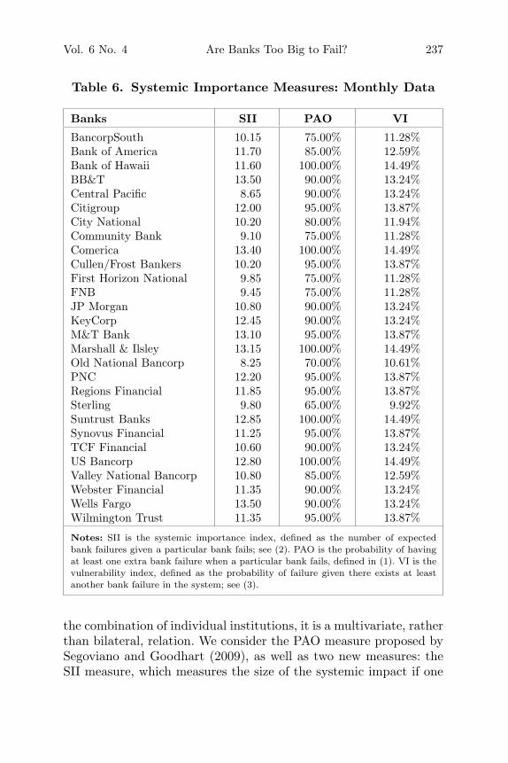
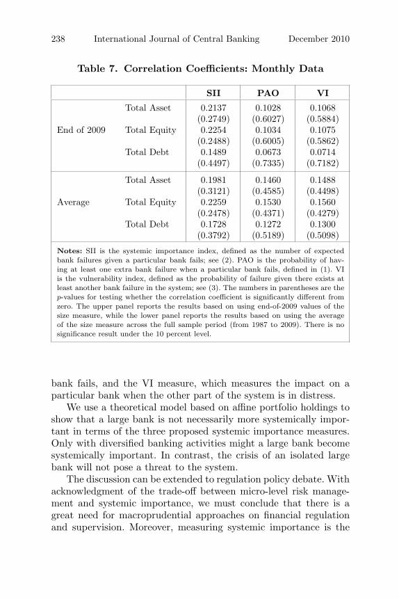
Last but not least, using daily equity returns may present apotential problem due to the heteroskedasticity in high-frequencyfinancial returns. Diebold, Schuermann, and Stroughair (2000) arguethat the fundamental assumption of EVT—that the observations areindependent and identically distributed (i.i.d.)—is usually violatedwhen dealing with high-frequency financial returns. They providetwo potential solutions: firstly, one may investigate low-frequencyblock maxima, which reduces the dependency across time; secondly,one may apply a conditional extreme value model. In line with thesecond type of solution, Chavez-Demoulin, Davison, and McNeil(2005) consider a point process approach to decluster the finan-cial return data. Notice that the non-i.i.d. problem is mainly forevaluating the univariate tail events. Because our study is under amultivariate framework, which models cross-sectional dependence oftail events, the non-i.i.d. problem on the time dimension is of lessconcern. Nevertheless, we conduct a robustness check in line withthe first type of solution proposed by Diebold, Schuermann, andStroughair (2000). Instead of daily returns, we consider monthlyreturns. Similar to the block maxima approach, considering monthlyreturns reduces the interdependent problem on the time dimension.Due to the low frequency, we have to use the full sample (276months) for the analysis. The results appear in table 6. The esti-mates of the three systemic risk measures are similar to those usingdaily returns—at least in terms of ranking the systemic importance.The absolute level is higher than that using daily returns, because itis more likely to observe simultaneous tail events in the same month.We repeat the Pearson correlation analysis as shown in table 7.Again, we confirm that the systemic importance measures are notcorrelated with the size measures.

6. Conclusion

This paper considers three measures of systemic importance of finan-cial institutions in a financial system. Since we regard the system as


Table 6. Systemic Importance Measures: Monthly Data

Banks SII PAO VI

BancorpSouth 10.15 75.00% 11.28%Bank of America 11.70 85.00% 12.59%Bank of Hawaii 11.60 100.00% 14.49%BB&T 13.50 90.00% 13.24%Central Pacific 8.65 90.00% 13.24%Citigroup 12.00 95.00% 13.87%City National 10.20 80.00% 11.94%Community Bank 9.10 75.00% 11.28%Comerica 13.40 100.00% 14.49%Cullen/Frost Bankers 10.20 95.00% 13.87%First Horizon National 9.85 75.00% 11.28%FNB 9.45 75.00% 11.28%JP Morgan 10.80 90.00% 13.24%KeyCorp 12.45 90.00% 13.24%M&T Bank 13.10 95.00% 13.87%Marshall & Ilsley 13.15 100.00% 14.49%Old National Bancorp 8.25 70.00% 10.61%PNC 12.20 95.00% 13.87%Regions Financial 11.85 95.00% 13.87%Sterling 9.80 65.00% 9.92%Suntrust Banks 12.85 100.00% 14.49%Synovus Financial 11.25 95.00% 13.87%TCF Financial 10.60 90.00% 13.24%US Bancorp 12.80 100.00% 14.49%Valley National Bancorp 10.80 85.00% 12.59%Webster Financial 11.35 90.00% 13.24%Wells Fargo 13.50 90.00% 13.24%Wilmington Trust 11.35 95.00% 13.87%

Notes: SII is the systemic importance index, defined as the number of expectedbank failures given a particular bank fails; see (2). PAO is the probability of havingat least one extra bank failure when a particular bank fails, defined in (1). VI is thevulnerability index, defined as the probability of failure given there exists at leastanother bank failure in the system; see (3).

the combination of individual institutions, it is a multivariate, ratherthan bilateral, relation. We consider the PAO measure proposed bySegoviano and Goodhart (2009), as well as two new measures: theSII measure, which measures the size of the systemic impact if one


Table 7. Correlation Coefficients: Monthly Data

SII PAO VI

Total Asset 0.2137 0.1028 0.1068(0.2749) (0.6027) (0.5884)

End of 2009 Total Equity 0.2254 0.1034 0.1075(0.2488) (0.6005) (0.5862)

Total Debt 0.1489 0.0673 0.0714(0.4497) (0.7335) (0.7182)

Total Asset 0.1981 0.1460 0.1488(0.3121) (0.4585) (0.4498)

Average Total Equity 0.2259 0.1530 0.1560(0.2478) (0.4371) (0.4279)

Total Debt 0.1728 0.1272 0.1300(0.3792) (0.5189) (0.5098)

Notes: SII is the systemic importance index, defined as the number of expectedbank failures given a particular bank fails; see (2). PAO is the probability of hav-ing at least one extra bank failure when a particular bank fails, defined in (1). VIis the vulnerability index, defined as the probability of failure given there exists atleast another bank failure in the system; see (3). The numbers in parentheses are thep-values for testing whether the correlation coefficient is significantly different fromzero. The upper panel reports the results based on using end-of-2009 values of thesize measure, while the lower panel reports the results based on using the averageof the size measure across the full sample period (from 1987 to 2009). There is nosignificance result under the 10 percent level.

bank fails, and the VI measure, which measures the impact on aparticular bank when the other part of the system is in distress.

We use a theoretical model based on affine portfolio holdings toshow that a large bank is not necessarily more systemically impor-tant in terms of the three proposed systemic importance measures.Only with diversified banking activities might a large bank becomesystemically important. In contrast, the crisis of an isolated largebank will not pose a threat to the system.

The discussion can be extended to regulation policy debate. Withacknowledgment of the trade-off between micro-level risk manage-ment and systemic importance, we must conclude that there is agreat need for macroprudential approaches on financial regulationand supervision. Moreover, measuring systemic importance is the


key to identifying systemically important institutions when imposingmacroprudential regulations.

Besides developing the theoretical model, we conduct an empir-ical analysis—using multivariate EVT—to estimate the systemicimportance measures. The empirical observation confirms that thePAO measure is not as informative as the SII measure in terms ofdistinguishing the systemically important banks. A moving windowanalysis shows similar results. Moreover, the VI measure is shownto be as informative as the PAO measure in terms of identifyingsystemically important banks.

We use the estimated systemic importance measures to testwhether they are correlated with the measures on bank size. Regard-ing the systemic impact of bank failure measured by the SII measure,there is no empirical evidence supporting the “too big to fail” argu-ment in terms of the Pearson correlation. In contrast, the other twosystemic importance measures, PAO and VI, are positively corre-lated to the size measures. When considering the Spearman corre-lation, we find support for “too big to fail.” Moreover, we find thatin the more recent period the correlations disappear, which suggeststhat particular attention should be given to the systemic importancemeasures in recent years.

The empirical analysis in this paper is based on an artificial banksystem. Therefore, the evidence from the empirical analysis shouldnot be regarded as either support or disproof of the “too big to fail”argument. The bottom line is that we show the possibility of havinga banking system in which the size measures are not a good proxyof the systemic importance.

Although in the current empirical analysis our proposed SIImeasure is shown to be more informative than the PAO measure pro-posed by Segoviano and Goodhart (2009), we address one potentialdrawback of the SII measure: it is a simple counting measure thattakes no account of the differences between potential losses whendifferent financial institutions fail. In other words, when calculatingthe expected number of failures in the system, the SII measure doesnot distinguish whether it causes a failure of a big bank or a smallbank. This could be improved by considering the expected totalloss in the system if one bank fails—i.e., calculating the expectedshortfall conditional on a certain bank failure, which incorporatesthe size of all banks. Acharya, Santos, and Yorulmazer (2010) have


designed systemic importance measures in this manner, while tak-ing the heavy-tailedness of individual returns into consideration. Tomodel the dependence structure, they use dynamic conditional cor-relation (DCC) models, which have an EVT flavor but deviate fromthe multivariate EVT framework. A systemic importance measureaddressing the conditional expected shortfall under the multivariateEVT framework may overcome the drawback of the proposed SIImeasure. This is left for future research.

Appendix 1. Proofs

Proof of Proposition 1

Recall the definition of the PAO measure in (1). We have that

PAOi(p) =P ({∃j �= i, s.t. Xj > V aRj(p)} ∩ {Xi > V aRi(p)})

P (Xi > V aRi(p))

=1pP ({∃j �= i, s.t. Xj > V aRj(p)}) + 1

− 1pP ({∃j �= i, s.t. Xj > V aRj(p)} ∪ {Xi > V aRi(p)})

=1pP ({∃j �= i, s.t. Xj > V aRj(p)}) + 1

− 1pP ({∃j, s.t. Xj > V aRj(p)})

=: I1 + 1 − I2.

From the definition of the L function in (4), as p → 0, I1 →L�=i(1, 1, . . . , 1) and I2 → L(1, 1, . . . , 1), which implies (6).


Recall the definition of the SII measure in (2). We have that

SIIi(p) =d∑

j=1

E(1Xj>V aRj(p)|Xi > V aRi(p))


=d∑

j=1

P (Xj > V aRj(p)|Xi > V aRi(p))

=d∑

j=1

P (Xj > V aRj(p), Xi > V aRi(p))P (Xi > V aRi(p))

=d∑

j=1

P (Xj > V aRj(p)) + P (Xi > V aRi(p))−P (Xj > V aRj(p) or Xi > V aRi(p))

p

=d∑

j=1

2 − P (Xj > V aRj(p) or Xi > V aRi(p))p

.

From the definition of the L function in (4), as p → 0,

P (Xj > V aRj(p) or Xi > V aRi(p))p

→ Li,j(1, 1).

The relation (8) is thus proved.

Proof of Corrollary 1

Since L(1, 1, . . . , 1) − 1 < 0, the relation (7) implies that ahigher value of the VI measure corresponds to a higher level ofL�=i(1, 1, . . . , 1). Together with (6), the corollary follows.

Proof of Theorem 1

Firstly, since the heavy-tailed feature in (11) assumes that the righttail of Yi dominates its left tail, it is sufficient to assume that Yi areall positive random variables for i = 1, 2, 3, i.e., without the left tail.We adopt this assumption in the rest of the proof.

We use the Feller convolution theorem to deal with the sum ofindependently heavy-tailed distributed random variables as in thefollowing lemma.

Lemma 2. Suppose positive random variables U and V are inde-pendent. Assume that they are both heavy-tailed distributed with thesame tail index α. Then, as s → ∞,


P (U + V > s) ∼ P (U > s) + P (V > s).

Notice that the heavy-tailed feature implies P (U > s)P (V >s) = o(P (U > s) + P (V > s)), as s → ∞. Hence, the Fellerconvolution theorem is equivalent to

P (U + V > s) ∼ P (max(U, V ) > s);

i.e., the sum and the maximum of two independently heavy-taileddistributed random variables are tail equivalent. A proof using setsmanipulation can be found in Embrechts, Kuppelberg, and Mikosch(1997). With an analogous proof under multivariate framework, amultivariate version of the Feller theorem can be obtained. In themultivariate case, the tail equivalence between two random vectorsis defined as the combination of having tail equivalence for eachmarginal distribution and having the same L function for the taildependence structure. We present the result in a two-dimensionalcontext in the following lemma without providing the proof.

Lemma 3. Suppose positive random variables U1 and U2 are inde-pendent. Assume that they are both heavy-tailed distributed with thesame tail index α. Then for any positive constants mij, 1 ≤ i, j ≤ 2,we have that the distribution functions of (m11U1 +m12U2, m21U1 +m22U2) and (m11U1 ∨ m12U2, m21U1 ∨ m22U2) are tail equivalent.

To prove theorem 1, it is necessary to calculate the L functionof (X1, X2, X3) on points (1, 1, 0), (1, 0, 1), and (0, 1, 1). The maininstrument in the calculation is lemma 3. We start by comparing theindividual risks taken by the three banks.

Proposition 4. For the three-bank model on (X1, X2, X3), asp → 0,

V aR2(p) = V aR3(p) ∼ cV aR1(p), (13)

where

c :=(

(2 − 2γ)α + 2γα

γα + μα + (1 − γ − μ)α

)−1/α

.



From lemma 2, we get that, as s → ∞,

P (X1 > s) ∼ P ((2 − 2γ)Y1 > s) + P (γY2 > s) + P (γY3 > s)

= ((2 − 2γ)α + 2γα)s−αK(s). (14)

Similarly, we get that

P (X2 > s) = P (X3 > s) ∼ (γα + μα + (1 − γ − μ)α)s−αK(s).(15)

By comparing (14) and (15), the relation (13) is a directconsequence.

We remark that c < 1. This is in line with the fact that the largebank X1 takes more risks than the small banks. Moreover, whenγ > 1/2, we get c > 1/2. In this case, the comparison between bankrisk taking is not proportional to the size. At a relative level, thesmall banks are taking more risk. In other words, the large bank X1benefits from diversification.

Next, we calculate L(1, 1, 0). Denote v(p) := V aR1(p). Fromlemma 3, we get that, as p → 0,

P (X1 > V aR1(p) or X2 > V aR2(p))

∼ P ((2 − 2γ)Y1 ∨ γY2 ∨ γY3 > v(p) or

γY1 ∨ (1 − γ − μ)Y2 ∨ μY3 > cv(p))

= P

(Y1 >

v(p)(2 − 2γ) ∨ γ

c

or Y2 >v(p)

γ ∨ 1−γ−μc

or Y3 >v(p)γ ∨ μ

c

)

∼ P

(Y1 >

v(p)(2 − 2γ) ∨ γ

c

)+ P

(Y2 >

v(p)γ ∨ 1−γ−μ

c

)

+ P

(Y3 >

v(p)γ ∨ μ

c

)

∼[(

(2 − 2γ) ∨ γ

c

)α

+(γ ∨ μ

c

)α

+(

γ ∨ 1 − γ − μ

c

)α]

× P (Y1 > v(p)). (16)


From (14), we get that p ∼ ((2−2γ)α +2γα)P (Y1 > v(p)) as p → 0.Together with (16) and (5), we have that

L(1, 1, 0) = limp→0

P (X1 > V aR1(p) or X2 > V aR2(p))p

=

((2 − 2γ) ∨ γ

c

)α +(γ ∨ μ

c

)α +(γ ∨ 1−γ−μ

c

)α

(2 − 2γ)α + 2γα. (17)

Due to the symmetry, we have that L(1, 0, 1) = L(1, 1, 0). Followinga similar calculation, we obtain that

L(0, 1, 1) =

(γc

)α + 2(

μ∨(1−γ−μ)c

)α

(2 − 2γ)α + 2γα. (18)

Proposition 3 implies that SII2 = SII3. Moreover, SII1 > SII2 if andonly if L(1, 1, 0) < L(0, 1, 1). Hence it is only necessary to comparethe values of the L function at the two points.

Denote

Q := ((2 − 2γ)α + 2γα)(L(1, 1, 0) − L(0, 1, 1)).

We study the sign of Q in order to compare the systemic importancemeasures SIIi, i = 1, 2, 3.

Case 1: 23 ≤ γ < 1

Since γ > 1/2, we have c > 1/2. Thus, γ1−γ > 2 > 1

c , which impliesthat

γ >1 − γ

c> max

(1 − γ − μ

c,μ

c

).

Therefore

Q =((

(2 − 2γ) ∨ γ

c

)α

+ 2γα)

−((γ

c

)α

+ 2(

μ ∨ (1 − γ − μ)c

)α)> 0.

Hence, SII1 < SII2 = SII3.


Case 2: γ = 1/2

In this case, we still have c ≥ 1/2. The equality holds if and onlyif μ = 1/4. Due to the symmetric position between X2 and X3,without loss of generality, we assume that μ ≤ 1/4. Then we getμ ≤ 1 − γ − μ. Moreover, the inequality μ/γ ≤ 1/2 ≤ c implies thatγ ≥ μ

c and it is not difficult to obtain that γ ≤ 1−γ−μc . Hence,

Q =(

1 + 2−α +(

1/2 − μ

c

)α)−

((γ

c

)α

+ 2(

1/2 − μ

c

)α)

= 1 + 2−α −(

12α

+(

12

− μ

)α)c−α

= 1 +12α

− 1 + (1 − 2μ)α

2α

2α + 21 + (2μ)α + (1 − 2μ)α

= 1 +12α

−(

1 +22α

) (1 − (2μ)α

1 + (2μ)α + (1 − 2μ)α

)

≤ 1 +12α

−(

1 +22α

) (1 − (1/2)α

1 + (1/2)α + (1/2)α

)

= 0.

Here we used the facts that (2μ)α

1+(2μ)α+(1−2μ)α is an increasing functionwith respect to μ and μ ≤ 1/4. The equality holds if and only if μ =1/4. Hence, in case γ = 1/2, we conclude that SII1 ≥ SII2 = SII3,with the equality holding if and only if μ = 1/4.

Case 3: 0 < γ ≤ 1/3

In this case, it is not difficult to verify that 2−2γ > γc and γ < 1−γ

2c .Due to the symmetry, we only consider the case 0 < μ ≤ 1−γ

2 . Thenwe have that μ ≤ 1 − γ − μ and γ < 1−γ−μ

c . Therefore

Q = (2 − 2γ)α +(γ ∨ μ

c

)α

− γα + (1 − γ − μ)α

cα. (19)

For any fixed γ, c is a function of μ denoted by c(μ). For 0 < μ <1−γ

2 , c(μ) is a strictly decreasing function. Thus g(μ) := μc(μ) is a

continuous, strictly increasing function. Notice that g(0) = 0 < γand g((1 − γ)/2) > γ. There must exist a unique μ∗ ∈ (0, (1 − γ)/2)such that g(μ∗) = γ.


Denote c∗ := c(μ∗). From μ∗

c∗ = γ, we get that

γα

μ∗α= (c∗)−α =

(2 − 2γ)α + 2γα

γα + μ∗α + (1 − γ − μ∗)α.

It implies that

γα

μ∗α= (c∗)−α =

(2 − 2γ)α + γα

γα + (1 − γ − μ∗)α.

Continuing from equation (19), we get that

Q(μ∗) = (2 − 2γ)α + γα − (γα + (1 − γ − μ∗)α)(c∗)−α = 0.

Hence, we conclude that for μ = μ∗, SII1 = SII2 = SII3.For 0 < μ < μ∗, it is clear that

Q(μ) = (2 − 2γ)α + γα − (γα + (1 − γ − μ)α)c−α

= (2 − 2γ)α + γα− (γα + (1 −γ − μ)α)(2 − 2γ)α + 2γα

γα + μα + (1− γ− μ)α

=((2 − 2γ)α + γα)μα − γα(γα + (1 − γ − μ)α)

γα + μα + (1 − γ − μ)α

is a strictly increasing function with respect to μ. Moreover, forμ∗ < μ < 1−γ

2 , Q is calculated as

Q(μ) = (2 − 2γ)α + (μα − γα − (1 − γ − μ)α)c−α

= (2 − 2γ)α + (μα− γα − (1 −γ − μ)α)(2 − 2γ)α + 2γα

γα + μα + (1− γ− μ)α

=2(2 − 2γ)αμα + 2γα(μα − γα − (1 − γ − μ)α)

γα + μα + (1 − γ − μ)α,

which is also a strictly increasing function with respect to μ. There-fore, for 0 < μ < μ∗, Q < 0 while for μ∗ < μ < 1−γ

2 , Q > 0.Correspondingly, we have SII1 > SII2 = SII3 in the former case andSII1 < SII2 = SII3 in the latter case.

Due to the symmetry, a similar result holds when 1−γ2 < μ <

1 − γ, and the switch point is then 1 − γ − μ∗. More specifically, for1−γ

2 < μ < 1 − γ − μ∗, SII1 < SII2 = SII3; and for μ = 1 − γ − μ∗,SII1 = SII2 = SII3; for 1 − γ − μ∗ < μ < 1 − γ, SII1 > SII2 = SII3.The theorem is thus proved for case 3.


Proof of Lemma 1

Along the lines of the proof of theorem 1, we obtained that in athree-bank model,

SII1 − SII2 = {1 + (2 − L(1, 1, 0)) + (2 − L(1, 0, 1))}− {(2 − L(1, 1, 0)) + 1 + (2 − L(0, 1, 1))}

= L(0, 1, 1) − L(1, 0, 1).

Therefore, SIIi > SIIj if and only if L�=i(1, 1, . . . , 1) >L �=j(1, 1, . . . , 1). Together with (6), the lemma is proved.

We remark that the above calculation is not based on the affineportfolio model. Hence, the result is valid in a general three-bankmodel. However, one cannot obtain similar relations when the num-ber of banks exceeds three.

Appendix 2. Statistical Estimation on the L Function

Consider independently and identically distributed (i.i.d.) observa-tions from the random vector (X1, . . . , Xd) denoted by

{(X1s, X2s, . . . , Xds)|1 ≤ s ≤ n}.

The sample size is n. The non-parametric approach of estimatingthe L function starts from the assumption (4). Roughly speaking,the estimation takes a certain p-value for which the VaR for eachdimension can be estimated by the order statistics. Then the proba-bility in the numerator of (4) is estimated by a counting measure. Toensure that p → 0, theoretically we take a sequence k := k(n), suchthat k(n) → ∞ and k(n)/n → 0 as n → ∞, and get an empiricalestimation of the L function from replacing p with k/n and using theempirical estimation on the distribution function of (X1, X2 . . . , Xd).The explicit estimator is given as

L(x1, . . . , xd) :=1k

n∑s=1

1∃1≤i≤d, s.t. Xis>Xi,n−[kxi],


where Xi,1 ≤ Xi,2 ≤ · · · ≤ Xi,n are the order statistics of the i -thdimension of the sample, Xi1, . . . , Xin, for 1 ≤ i ≤ d. Particularly,L(1, 1, . . . , 1) is estimated by

L(1, 1, . . . , 1) :=1k

n∑s=1

1∃1≤i≤d, s.t. Xis>Xi,n−k.

For the estimator of the L function, usual statistical properties,such as consistency and asymptotic normality, have been proved.See, e.g., de Haan and Ferreira (2006).

Practically, the theoretical conditions on k are not relevant for afinite sample analysis. Thus, how to choose a proper k in the esti-mator is a major issue in estimation. Instead of taking an arbitraryk, a usual procedure is to calculate the estimator of L(1, 1, . . . , 1)under different k values and draw a line plot against the k val-ues. With a low k value, the estimation exhibits a large variance,while for a high k value, since the estimation uses too many obser-vations in the moderate level, it bears a potential bias. Therefore,k is usually chosen by picking the first stable part of the line plotstarting from low k, which balances the trade-off between the vari-ance and the bias. The estimates follow from the k choice. Becausek is chosen from a stable part of the line plot, a small variationof the k value does not change the estimated value. Thus, theexact k value is not sensitive for the estimation on the L function.Such a procedure has been applied in univariate EVT for tail indexestimation.

With the chosen k, we in fact consider a tail event as the lossreturn exceeds a VaR with tail probability level k/n. In our empiricalapplication, the chosen k value differs according to the sample size.For the full sample analysis (sample size 6,000), we choose k = 180,which corresponds to a p level at 3 percent; for the moving windowanalysis (sample size 2,000), we choose k = 100, which correspondsto p = 5%; for the monthly data analysis (sample size 276), wechoose k = 20, which corresponds to p = 7.2%. With a lower num-ber of observations, we choose a slightly higher level of p, albeit ina low absolute level.


References

Acharya, V. V., J. A. C. Santos, and T. Yorulmazer. 2010.“Systemic Risk and Deposit Insurance Premiums.” EconomicPolicy Review (Federal Reserve Bank of New York) 16 (1):89–98.

Acharya, V. V., and T. Yorulmazer. 2007. “Too Many to Fail—An Analysis of Time-Inconsistency in Bank Closure Policies.”Journal of Financial Intermediation 16 (1): 1–31.

Adrian, T., and M. Brunnermeier. 2008. “CoVaR.” Federal ReserveBank of New York Staff Report No. 348.

Allen, F., E. Carletti, and A. Babus. 2009. “Financial Crises: The-ory and Evidence.” Annual Review of Financial Economics 1(1): 97–116.

Allen, F., and D. Gale. 2000. “Financial Contagion.” Journal ofPolitical Economy 108: 1–33.

Bernanke, B. 2009. “Financial Reform to Address Systemic Risk.”Speech at the Council on Foreign Relations, Washington, DC,March 10.

Chavez-Demoulin, V., A. C. Davison, and A. J. McNeil. 2005. “Esti-mating Value-at-Risk: A Point Process Approach.” QuantitativeFinance 5 (2): 227–34.

Cifuentes, R., H. S. Shin, and G. Ferrucci. 2005. “Liquidity Riskand Contagion.” Journal of the European Economic Association3 (2–3): 556–66.

Dasgupta, A. 2004. “Financial Contagion through Capital Connec-tions: A Model of the Origin and Spread of Bank Panics.” Journalof the European Economic Association 2 (6): 1049–84.

De Bandt, O., and P. Hartmann. 2001. “Systemic Risk in Banking:A Survey.” In Financial Crisis, Contagion, and the Lender ofLast Resort: A Reader, ed. C. Goodhart and G. Illing, 249–98.Oxford University Press.

De Haan, L., and A. Ferreira. 2006. Extreme Value Theory: AnIntroduction. Springer.

De Vries, C. G. 2005. “The Simple Economics of Bank Fragility.”Journal of Banking and Finance 29 (4): 803–25.

Diebold, F. X., T. Schuermann, and J. D. Stroughair. 2000. “Pitfallsand Opportunities in the Use of Extreme Value Theory in RiskManagement.” Journal of Risk Finance 1 (2): 30–35.


Diebold, F. X., and K. Yilmaz. 2009. “Measuring Financial AssetReturn and Volatility Spillovers, with Application to GlobalEquity Markets.” Economic Journal 119 (534): 158–71.

Embrechts, P., C. Kluppelberg, and T. Mikosch. 1997. ModellingExtremal Events: for Insurance and Finance. Springer.

Freixas, X., B. M. Parigi, and J.-C. Rochet. 2000. “Systemic Risk,Interbank Relations, and Liquidity Provision by the CentralBank.” Journal of Money, Credit, and Banking 32 (3): 611–38.

Hartmann, P., S. Straetmans, and C. G. de Vries. 2004. “AssetMarket Linkages in Crisis Periods.” Review of Economics andStatistics 86 (1): 313–26.

———. 2005. “Banking System Stability: A Cross-Atlantic Perspec-tive.” NBER Working Paper No. 11698.

International Monetary Fund. 2009. Global Financial StabilityReport (April).

Lagunoff, R., and S. L. Schreft. 2001. “A Model of FinancialFragility.” Journal of Economic Theory 99 (1): 220–64.

Poon, S., M. Rockinger, and J. Tawn. 2004. “Extreme Value Depen-dence in Financial Markets: Diagnostics, Models, and FinancialImplications.” Review of Financial Studies 17 (2): 581–610.

Rajan, R. G. 2009. “Too Systemic to Fail: Consequences, Causes andPotential Remedies.” Written statement to the Senate BankingCommittee Hearings, May 6.

Segoviano, M., and C. Goodhart. 2009. “Banking Stability Meas-ures.” IMF Working Paper No. 09/04.

Stern, G. H., and R. J. Feldman. 2004. Too Big to Fail: The Hazardsof Bank Bailouts. Brookings Institution Press.

Zhou, C. 2008. On Extreme Value Statistics. PhD Thesis, TinbergenInstitute.

Documents

Are Banks Too Big to Fail? Measuring Systemic Importance ... · Are Banks Too Big to Fail? Measuring Systemic Importance of Financial Institutions∗ Chen Zhou De Nederlandsche Bank