Are Product Spreads Useful for Forecasting Oil Prices?

An Empirical Evaluation of the Verleger Hypothesis∗

Christiane Baumeister Lutz Kilian†

Bank of Canada University of Michigan

CEPR

Xiaoqing Zhou

University of Michigan

September 18, 2014

Abstract

Notwithstanding a resurgence in research on out-of-sample forecasts of the price of oil in

recent years, there is one important approach to forecasting the real price of oil which has not

been studied systematically to date. This approach is based on the premise that demand for

crude oil derives from the demand for refined products such as gasoline or heating oil. Oil indus-

try analysts such as Philip Verleger and financial analysts widely believe that there is predictive

power in the product spread, defined as the difference between suitably weighted refined product

market prices and the price of crude oil. Our objective is to evaluate this proposition. We derive

from first principles a number of alternative forecasting model specifications involving product

spreads and compare these models to the no-change forecast of the real price of oil. We show

that not all product spread models are useful for out-of-sample forecasting, but some models

are, even at horizons between one and two years. The most accurate model is a time-varying

parameter model of gasoline and heating oil spot price spreads that allows for structural change

in product markets. We document MSPE reductions as high as 20% and directional accuracy

as high as 63% at the two-year horizon, making product spread models a good complement to

forecasting models based on economic fundamentals, which work best at short horizons.

JEL: Q43, C53, G15

KEYWORDS: Oil price; Futures; WTI; Brent; Acquisition Cost; Refined products; Crack spread;

Forecast accuracy; Real-time data.

∗We thank Ron Alquist, Bahattin Büyüksahin, Barbara Rossi, and Philip K. Verleger for helpful comments andJonathan Wright for providing access to his data. Jamshid Mavalwalla provided excellent research assistance. The

views in this paper are solely the responsibility of the authors and should not be interpreted as reflecting the views

of the Bank of Canada.†Corresponding author: Lutz Kilian, University of Michigan, Department of Economics, 309 Lorch Hall, Ann

Arbor, MI 48109-1220. E-mail: lkilian@umich.edu.

1 Introduction

Oil price forecasts affect the economic outlook of oil-importing as well as oil-exporting countries.

Accurate oil price forecasts are required, for example, to guide natural resource development and

investments in infrastructure. They also play an important role in preparing budget and investment

plans. Users of oil price forecasts include international organizations, central banks, governments

at the state and federal level as well as a range of industries including utilities and automobile

manufacturers.

In recent years there has been a resurgence in research on the question of how to forecast the

price of commodities in general and the price of oil in particular, at least at horizons up to a year or

two. One strand of this literature has examined in depth the predictive power of oil futures prices

(see, e.g., Knetsch 2007; Alquist and Kilian 2010; Reeve and Vigfusson 2011; Alquist, Kilian and

Vigfusson 2013). Another strand of the literature has focused on the predictive content of changes

in oil inventories, oil production, macroeconomic fundamentals, and exchange rates (see, e.g., Chen,

Rogoff, and Rossi 2010; Baumeister and Kilian 2012; 2014a,b; Alquist, Kilian and Vigfusson 2013).

A third strand has looked at the forecasting ability of professional and survey forecasts (see, e.g.,

Sanders, Manfredo, and Boris 2008; Alquist, Kilian and Vigfusson 2013, Bernard, Khalaf, Kichian,

and Yelou 2013). The emerging consensus from this literature is that economic fundamentals help

forecast the real price of oil, at least during times of large and persistent movements in economic

fundamentals, but only at short horizons. In contrast, the forecasting ability of monthly and quar-

terly judgmental forecasts, and survey expectations tends to be low and that of oil futures prices

mixed at best.

It may seem that these studies would cover the universe of widely used predictors for the price of

oil. There is, however, another important approach to forecasting the real price of oil which has not

been studied systematically to date. This alternative approach is based on the premise that demand

for crude oil derives from the demand for refined products such as gasoline or heating oil.1 The

idea of derived demand has a long tradition in academic research on oil markets (see, e.g., Verleger

1982; Lowinger and Ram 1984). For example, Verleger (1982) advocates that spot market prices for

petroleum products are the primary determinants of crude oil prices, allowing one to express the

price of crude oil as a weighted average of refined product prices. A common view is that refiners

view themselves as price takers in product markets and cut their volume of production when they

cannot find crude oil at a price commensurate with product prices. In time, this reduction in the

demand for crude oil will lower the price of crude oil and the corresponding reduction in the supply

1The nature of this final demand is left unspecified. Changes in final demand may reflect business cycle fluctuations

or shifts in consumer preferences, for example. For further discussion also see Kilian (2010).

1

of products will boost product prices (see Verleger 2011). This reasoning suggests that the difference

between refined product market prices and the purchase price of crude oil should have predictive

power for the price of crude oil. We refer to this hypothesis as the Verleger hypothesis, given its

antecedents in Verleger’s work, but note that this view is widespread among oil industry analysts.

For example, energy consultant Kent Moors interprets crack spreads as market oil price expectations

and forecasts higher oil prices based on increasing gasoline spreads and heating oil spreads (see Moors

2011). Similarly, Goldman Sachs in April 2013 cut its oil price forecast citing significant downward

pressure on product spreads, which it interpreted as an indication of reduced demand for products

(see Strumpf 2013).

The same reasoning also plays an important role in financial markets. It is common to trade

futures contracts and options based on crack spreads (see, e.g., Haigh and Holt 2002; Chicago

Mercantile Exchange 2012). The crack spread refers to the approximate ratio in which refined

products such as gasoline or heating oil are produced from crude oil. There is not one single crack

spread that applies to all refineries, but the most commonly used ratio is 3:2:1, which refers to

refiners’ ability to produce two barrels of gasoline and one barrel of heating oil from three barrels

of crude oil. Because the spread between crude prices and refined product prices is the main driver

of refinery profit margins, futures contracts and options have been established to allow refining

companies to hedge their price risk related to the crack spread. Traders express the crack spread in

terms of futures prices of a given maturity as

2

3+ +

1

3 + − 1

+

where all date futures prices have been expressed in dollars per barrel (see Figure A1 in the not-

for-publication appendix). An obvious question of interest is whether the information contained in

product price spreads (also known as product margins) may be used to improve on the no-change

forecast of the price of crude oil, as is widely believed in the industry. For example, Evans (2009)

cites the oil market analyst Philip K. Verleger as forecasting a decline in the price of oil based on a

weakening 3:2:1 crack spread on the NYMEX.

Although there is a large literature relying on error correction models of the relationship between

oil prices and product prices, few studies to date have examined the problem of forecasting the price

of oil out of sample and none of those studies evaluates the out-of-sample forecast accuracy of

product spread models against the no-change forecast, making it difficult to interpret these results.2

2For example, the one-week ahead analysis of the predictive power of the 3:2:1 crack spread during 2000-08 in

Murat and Tokat (2009) is not conducted out of sample, as their discussion of the results might suggest, but is based

on full-sample regression estimates.

2

Moreover, existing studies limit their attention to forecast horizons of one month only and rely on

forecast evaluation periods that are too short to be informative. A case in point is the analysis in

Lanza, Manera, and Giovannini (2005).

The objective of our paper is to investigate systematically and in real time the forecasting power

of product spreads for the real price of oil. Our evaluation period extends from early 1992 until

September 2012. We derive a number of alternative model specifications based on the notion that

the price of oil can be expressed as a weighted average of product prices. We follow most industry

analysts in focusing on the prices for gasoline and heating oil. The four basic forecasting approaches

considered include: (1) the crack spread model, (2) models of individual product spreads, (3) the

weighted product spread model expressed relative to the current spot price of oil, and (4) equal-

weighted forecast combinations of individual product spread models. Our analysis also distinguishes

between spot and futures prices and explores the benefit of additional parameter restrictions, re-

sulting in the most comprehensive analysis of these models to date. The maximum forecast horizon

considered is 24 months in line with the needs of applied forecasters at central banks and at the U.S.

Energy Information Administration (EIA). We compare the out-of-sample accuracy of each of the

forecasting models to the no-change forecast of the real price of oil. This random walk benchmark

is widely used in the literature. Indeed, some observers have questioned whether it is possible to

forecast the price of oil with any degree of accuracy at all.3

We find that not all product spread models are useful for out-of-sample forecasting, but some

models yield statistically significant MSPE reductions as large as 6% at horizons between one and

two years. This result is noteworthy in that to date no other forecasting method has been able to

beat the no-change forecast of the real price of oil at horizons between one and two years (see, e.g.,

Baumeister and Kilian 2012, 2014b). The most accurate single-spread forecasting model overall is a

model based on the gasoline spot spread alone. Heating oil spreads are far less accurate predictors

than gasoline spreads. Weighted product spread models are never more accurate than gasoline spread

models. Perhaps surprisingly, there is no evidence of forecasting models based on the commonly

cited 3:2:1 crack spread having out-of-sample forecasting ability.

In addition to these models, we also explore forecast combinations based on rolling or recursive

inverse MSPE weights that adapt over time to each predictor’s recent forecast performance. The

latter approach allows us to address concerns, expressed in Verleger (2011), that the marginal market

that determines the price of crude oil in models of derived demand tends to evolve over time.

For example, whereas the marginal product market for many years was the gasoline market, more

3For example, Peter Davies, chief economist of British Petroleum, has taken the position that “we cannot forecast

oil prices with any degree of accuracy over any period whether short or long” (see Davies 2007).

3

recently the market for diesel and heating oil has evolved into the marginal market, according to

Verleger. For the same reason we also investigate the usefulness of time-varying parameter (TVP)

forecasting models for linear combinations of the gasoline and heating oil spreads. While there is

no indication that forecast combinations are more accurate than the gasoline spread model alone, a

suitably restricted TVP model yields further improvements in out-of-sample forecast accuracy. This

TVP model is more accurate than the random walk model at all forecast horizons we consider. We

document MSPE reductions as high as 20% and directional accuracy as high as 66%, making this

specification the most useful forecasting approach overall.

The remainder of the paper is organized as follows. Section 2 discusses the data and describes

the forecasting environment. In section 3, we derive the main forecasting models. Section 4 contains

the out-of-sample results for alternative oil price measures. In section 5, we relax the assumptions

underlying conventional product spread models by allowing for smooth structural change. We also

consider extensions to European oil and product prices as well as global forecasting models. We

conclude in section 6. Additional results are contained in a not-for-publication appendix.

2 The Forecasting Environment

Our objective is to compare the real-time out-of-sample forecast accuracy of selected product spread

models for the average monthly real price of crude oil. The focus on the average price is consistent

with the objective of government agencies reporting oil price forecasts. The focus on the real price

of oil is standard in the literature because it is the real price of oil that matters for economic decision

making. Extensions to the problem of forecasting the nominal price of oil are straightforward and

are discussed in the not-for-publication appendix. Our baseline analysis focuses on the monthly

average of the West Texas Intermediate (WTI) spot price as reported in the FRED database of the

Federal Reserve Bank of St. Louis. This price refers to the U.S. dollar price of a barrel of a type

of crude oil known as West Texas Intermediate for immediate delivery in Cushing, Oklahoma. WTI

prices are commonly used as reference prices in writing contracts for the delivery of crude oil and

are available in real time.

We also report an alternative set of results for the monthly U.S. refiners’ acquisition cost for

crude oil imports, which refers to the average U.S. dollar price per barrel paid by U.S. refineries

for crude oil imported from abroad. The U.S. refiners’ acquisition cost for crude oil imports is a

better proxy for the global price of crude oil than the WTI price. It is reported in the Monthly

Energy Review of the U.S. EIA. Unlike the WTI price it is available only with a delay and subject

to revisions. Real-time data for the refiners’ acquisition cost since July 1986 were obtained from

4

the real-time database of Baumeister and Kilian (2012), suitably updated to include vintages from

January 1991 until March 2013. Both crude oil price series were deflated using the real-time U.S.

consumer price index for all urban consumers from the same database.

The crude oil price predictors considered below rely on spot and futures prices for gasoline,

heating oil and WTI crude oil. All predictors are available without delay and are not subject to

revisions. The price of WTI crude oil futures is from Bloomberg. Averages of daily futures prices

at maturities of 1 to 6 months are available starting in July 1986.

The futures contract for conventional regular unleaded gasoline for delivery in New York Harbor

ceased trading after the January 2007 contract. Starting in October 2005, it was replaced by a

gasoline futures contract for reformulated blendstock for oxygenate blending (RBOB) for delivery

in New York Harbor. We use the futures price for regular gasoline from July 1986 until December

2005 and the futures price of RBOB gasoline from January 2006 onwards. Daily gasoline futures

prices are available at maturities of 1, 3, and 6 months from Bloomberg. We construct monthly

averages, starting in July 1986 for 1- and 3-month contracts and starting in November 1986 for

6-month contracts, by averaging the daily futures prices. The corresponding spot price for delivery

of regular gasoline in New York Harbor is obtained from the EIA. This series is available for the

entire period of July 1986 until March 2013. There is no RBOB spot price series for delivery in

New York, making it impossible to construct a gasoline spot price the same way as for the futures

contracts.

Futures contracts for No. 2 Heating Oil are also for delivery in New York Harbor. We constructed

averages of the daily futures price data provided by Bloomberg. For maturities of 1 through 9

months the sample starts in July 1986; for the 12-month maturity it starts in August 1989. The

corresponding spot price since July 1986 is constructed as the average of the daily heating oil spot

price provided by the EIA.

Whereas crude oil prices are reported in U.S. dollars per barrel, gasoline and heating oil prices

are reported in cents per gallon. All product prices are transformed to dollars per barrel, which

involves multiplying each product price by 42 gallons/barrel and dividing by 100 cents/dollar.

Yet another common benchmark for oil prices is the price of Brent crude oil, which refers to

a grade of North Sea oil traded on the Intercontinental Exchange (ICE) in London. Some of our

extensions in section 5 rely on data for the spot price of Brent crude oil provided by Argus Media.

These data start in January 1990 and are backcast using Brent spot prices from the Intercontinental

Exchange (ICE) and the growth rate of the WTI price. The best proxy for the European product

market is the Rotterdam market. Daily product prices for the Rotterdam market are also provided

by Argus Media, starting in January 1990. The heating oil spot price series is backcast using the rate

5

of change in the price of New York Harbor No. 2 Heating Oil. The corresponding Rotterdam gasoline

spot price series only starts in 2005, which is too short for our purposes. Similarly, there are no

suitable time series for Rotterdam product futures prices. All prices are converted to dollars/barrel,

as appropriate. The raw data are expressed in dollars/metric ton. One metric ton corresponds to

7.5 barrels of crude oil. Monthly data are constructed by taking averages of the daily data.

The forecast evaluation period runs from January 1992 to September 2012. To the extent that

forecasting models are estimated, the model estimates are updated recursively, as is standard in the

oil price forecasting literature (see, e.g., Baumeister and Kilian 2012, 2014b). The reason is that

forecasts of the real price of oil based on rolling regressions are systematically less accurate than

forecasts based on recursive regressions, as shown in the not-for-publication appendix. We forecast

the ex-post revised real price of oil in levels rather than in logs. Real oil prices from the March 2013

vintage of real-time data are used to proxy for the ex-post revised data, against which all forecasts

are evaluated.

Our objective is to assess the real-time out-of-sample forecasting ability of models based on prod-

uct price spreads. We evaluate the forecasts in question in terms of their mean-squared prediction

error (MSPE) relative to the no-change forecast of the real price of oil and based on their directional

accuracy. Under the null hypothesis of no directional accuracy, the success ratio of the model at

predicting the direction of change in the price of oil should be no better than tossing a fair coin

with success probability 0.5. Tests of the null of no directional accuracy are conducted using the

test of Pesaran and Timmermann (2009). Where appropriate, we assess the statistical significance

of the MSPE reductions based on the test of Diebold and Mariano (1995) for nonnested models

without estimation uncertainty or based on the test of Clark and West (2007) for nested models

with estimation uncertainty.4

3 Forecasting Models

In this section, the forecasting models to be evaluated in sections 4 and 5 are derived. Some of these

models are already used in practice or have been discussed in the literature, while others are new.

4The latter test (like similar tests in the literature) is biased toward rejecting the null of equal MSPEs because it

tests the null of no predictability in population rather than the null of equal out-of-sample MSPEs (see Inoue and

Kilian 2004). It also ignores the real-time nature of the inflation data used in our forecasting exercise (see Clark and

McCracken 2009). Thus, these test results have to be viewed with caution. The alternative test of Giacomini and

White (2006) does not apply either in our context because it does not allow for recursive estimation. For further

discussion of the problem of out-of-sample inference see Kilian (2014).

6

3.1 The Benchmark Model

The benchmark model for the forecast accuracy comparisons in this paper is a random walk model

without drift. This model implies that the best forecast of the future price of crude oil is the current

price of crude oil. It also implies that the direction of change in the price of oil is unforecastable

such that the probability of the price of crude oil increasing equals that of the price of crude oil

decreasing. In other words, the model implies the no-change forecast

\+|=

where denotes the current monthly real price of crude oil. This benchmark is standard in the

literature on forecasting oil prices and more generally in the literature on forecasting asset prices.

The question of interest in this paper is whether alternative forecasting models based on the spread

of refined product prices over the price of crude oil may outperform this benchmark.

3.2 Verleger’s Decomposition

The idea of using petroleum product prices to explain the price of crude oil dates back to Verleger

(1982) who noted that the value of a barrel of crude oil at time can be expressed as a weighted

average of the nominal market prices, , of the principal products of a refiner:

=

X=1

(1)

where the weights reflect technological constraints. The nominal dollar price of a barrel of

crude oil a refiner is willing to pay in a competitive market, or the spot price of crude oil, ,

corresponds to this value adjusted for transportation costs, , and the refining costs, :

= − − (2)

These costs are typically treated as a constant in empirical work. From this relationship, we may

infer that, up to a constant,

=

X=1

and hence

7

+ =

X=1

+ (3)

where + is the spot price of product at + .

Verleger (2011) discusses how to use the static model embodied in equation (3) to predict the

price of oil. It is important to stress that Verleger’s objective is not to forecast the price of oil, as the

term prediction may seem to suggest, but rather to explain the evolution of the price of oil in terms

of that of the contemporaneous product prices. In contrast, our objective in this paper is to derive

from Verleger’s decomposition suitable forecasting models that can be implemented in real time to

generate out-of-sample forecasts. As we show below, there are several alternative specifications that

can be derived from equation (3).

3.3 Using Product Futures Spreads

Given date information, the conditional expectation of (3) is:

E +| =

X=1

E +| (4)

In the absence of a risk premium, arbitrage ensures that the expectation of the spot market price

for product equals the current futures price of product :

E +| =

+ = 1 (5)

Combining equations (4) and (5) yields:

E +| =

X=1

+ (6)

where + is the futures price of product in period with maturity periods. Dividing both

sides of equation (6) by , and taking logs on both sides, we obtain:

log

ÃE +|

!= log

ÃX=1

+

!− log

(7)

Using the approximation log(1 + ) ≈ , equation (7) can be expressed as:

E³+| −

´= log

ÃX=1

+

!− (8)

8

where lower case letters denote the natural log of prices. Equation (8) suggests the regression model

4+| = +

"log

ÃX=1

+

!−

#+ + (9)

where and are estimated recursively by the method of least squares and 4+| = +|− .

This motivates the forecasting model:

\+|=

exp

(+

"log

ÃX=1

+

!−

#)(10)

which implies that we can forecast the real price of crude oil as:

\+|=

exp

(+

"log

ÃX=1

+

!−

#− E(+)

)(11)

where + denotes the inflation rate from to + .

In practice, we approximate E(+) by the recursively estimated average inflation rate since

July 1986. The rationale for discarding the earlier data is that by 1991.12, it was readily apparent

that the Volcker disinflation of the early 1980s had succeeded by mid-1986. The not-for-publication

appendix shows that our forecast accuracy results for the real price of oil remain virtually unchanged,

if we replace this inflation forecast by a forecast from the fixed- inflation gap model of Faust and

Wright (2013), which has been shown to be the most accurate model-based inflation forecast.

3.3.1 The Single Futures Spread Model

We first propose the single futures spread model for product where { }. Itimmediately follows from equation (11) with either 0 or 1 that

\+|

= exp

n+

£ + −

¤− E(+)o (12)

where + is the log of the futures price of product at time with maturity periods.

3.3.2 The Crack Spread Futures Model

It is important to recognize that refined products are produced from a barrel of crude oil in ap-

proximately fixed proportions. In characterizing the refining process, it is common to ignore less

important refined products such as jet fuel and to focus on gasoline and heating oil only.5 Refining

5The reason is that the market traditionally has been concerned with forecasting the price of light sweet crude oil

which produces little residual fuel.

9

crude oil typically involves producing two barrels of gasoline and one barrel of heating oil from

three barrels of crude oil, resulting in a so-called crack spread of 3:2:1.6 Participants in mercantile

exchanges rely on the crack spread expressed in terms of the date futures prices with maturity :

+ ≡

2

3+ +

1

3+ −

+ (13)

where all prices are expressed in dollars per barrel, + denotes the date futures price of gasoline

of maturity and + denotes the date futures price of heating oil of maturity . Note that this

spread differs from the spread defined in equation (11). Whereas in one case we normalize relative

to the current spot price, in the other case we normalize relative to the current futures price.

A common view in financial markets is that the crack spread is the expected change in the spot

price of crude oil (see, e.g., Evans 2009). This view has been articulated by Verleger (2011), for

example. Verleger appeals to a model, in which refiners view themselves as price takers in product

markets and cut their volume of production when they cannot find crude oil at an expected price

commensurate with expected product prices. As Verleger explains, in time, this reduction in the

demand for crude oil will lower the spot price of crude oil and the corresponding reduction in the

supply of product will boost product prices. This reasoning suggests that the difference between

refined product market futures prices and the purchase price of crude oil for delivery in the near

future should have predictive power for the spot price of crude oil and motivates the forecasting

model:

\+|=

exp

½+

∙log

µ2

3+ +

1

3+ −

+

¶¸− E(+)

¾ (14)

3.3.3 The Weighted Product Futures Spread Model

Despite its popularity, the crack spread forecasting model (14) cannot be derived from (3) and is not

related to specification (11). Thus, there is no reason to expect model (14) to work well in practice.

In contrast, an alternative specification that can be formally derived from (3) and that is similar in

spirit to the Verleger model is obtained by setting 1 = 23 and 2 = 13 in the forecasting model

(11), resulting in

\+|=

exp

½+

∙log

µ2

3+ +

1

3+

¶−

¸− E(+)

¾ (15)

6Other common crack spread ratios are 5:3:2 and 2:1:1, depending on the type of refining process.

10

3.3.4 Equal-weighted Combination of Single Product Futures Spread Models

Finally, a more flexible approach to combining information from single product spreads is to assign

equal weight to the gasoline and heating oil futures spread forecasts:

\+|=1

2

2X=1

\+|

(16)

The motivation for this approach is that, even if one forecasting model by itself is more accurate

than the other, the less accurate model may still have additional predictive information not contained

in the more accurate model, allowing one to improve on the forecast accuracy of the more accurate

model by taking a weighted average of the two forecasts.

3.4 Using Product Spot Spreads

An alternative approach to deriving a product spread model is to postulate cointegration between

product spot prices and the spot price of crude oil such that log¡P

=1

¢ − ∼ (0). It is

well known that gasoline prices and crude oil prices, for example, move together in the long run

(see, e.g., Lanza et al. 2005; Kilian 2010). This cointegration relationship may be motivated, for

example, based on a model in which refiners are price takers in the crude oil market, as suggested by

Brown and Virmani (2007). As in typical long-horizon regressions used in empirical finance, under

the maintained hypothesis of cointegration, current deviations of suitably weighted spot prices of

refined products from the spot price of crude oil would be expected to have predictive power for

changes in the spot price of crude oil (see, e.g., Mark 1995; Kilian 1999):

4+| = +

"log

ÃX=1

!−

#+ +

The same cointegration relationship may also be motivated based on a model in which refiners

are price takers in the product market, as suggested by Verleger (2011). Recall equation (3)

E +| =

X=1

E +|

and replace the expected product prices by no-change forecasts. After taking logs and subtracting

from both sides, we obtain:

4+| = +

"log

ÃX=1

!−

#+ + (17)

11

allowing us to forecast the real price of oil as:

\+|=

exp

(+

"log

ÃX=1

!−

#− E(+)

)(18)

As in section 3.3, there are several special cases.

3.4.1 The Single Spot Spread Model

When = 1, the single product spot spread model is

\+|=

exph+

¡ −

¢− E(+)i (19)

where { }.

3.4.2 The Weighted Product Spot Spread Model

Similarly, we can derive from (19) the weighted product spot spread model:

\+|=

exp

½+

∙log

µ2

3 +

1

3

¶−

¸− E(+)

¾ (20)

3.4.3 Equal-weighted Combination of Single Product Spot Spread Models

As in the case of futures spreads, we also explore equal-weighted combinations of the forecasts based

on gasoline and heating oil spot spreads:

\+|=1

2

2X=1

\+|

(21)

4 Baseline Results

The models considered for the forecast comparison include a large number of forecasting models

based on various product futures price spreads and product spot price spreads, the predictive ability

of which we examine below.

4.1 Real WTI

We start our analysis with the results for the real WTI price. Table 1 presents the results for futures

product spreads and Table 2 shows the corresponding results for the product spot spreads. In all

12

cases, the product spreads are constructed by relating the product price to the corresponding WTI

price of crude oil.

4.1.1 Futures Spreads

The first five columns of Table 1 show the results for product futures spread models based on b andb. There are no statistically significant gains in directional accuracy for any model, but there is someevidence of MSPE reductions. For example, the gasoline spread model is about as accurate as the

no-change forecast at horizon 1, but more accurate at horizons 3 and 6. At the latter horizon, the

reduction in the MSPE by 10% is statistically significant at the 10% level. On the other hand, the

heating oil spread model has higher MSPEs than the no-change forecast at all horizons by as much

as 11%. The equal-weighted forecast combination of the gasoline and heating oil spread forecasts is

somewhat less accurate than the gasoline spread forecast, but the reduction in the MSPE at horizon

3 is more precisely estimated and statistically significant at the 5% level. The weighted product

spread is even less accurate than the equal-weighted forecast combination, but also statistically

significant at the 5% level at horizon 3. In contrast, there are no gains in forecast accuracy when

using the widely cited futures crack spread. We conclude that the best forecasting model is the

gasoline spread model.

The next five columns of Table 1 explore whether restricting the intercept of the spread models

to zero increases the forecast accuracy. This intercept reflects transportation costs and refining

costs, as discussed earlier. To the extent that these costs are small, one would expect an exclusion

restriction on the intercept to trade off forecast variance for forecast bias, potentially resulting in

a lower MSPE. Table 1 confirms this conjecture. Not only does the gasoline futures spread yield

reductions in the MSPE at all horizons, once = 0 is imposed, but the model also has improved

directional accuracy. The relative accuracy of alternative models compared with the gasoline futures

spread is not affected. An additional reason for imposing this restriction is that the unrestricted

estimate of often is negative, which is inconsistent with the underlying economic model.

We conclude that the gasoline futures spread model with = 0 imposed is the preferred fore-

casting model and much more accurate than models that combine information about gasoline and

heating oil futures prices, including the futures crack spread. The latter result is likely to be surpris-

ing to practitioners who rely on the crack spread, but was to be expected in light of the discussion

in section 3. We also obtained very similar results for the crack spread model when forecasting the

nominal oil price instead of the real price of oil, for example, or when replacing the log specification

for the crack spread by a levels specification.

13

4.1.2 Spot Spreads

An obvious limitation of the results in Table 1 is that we cannot forecast beyond six months, except

when using the heating oil spread which has no predictive power for the real price of oil at any

horizon. This observation motivates a closer examination of the product spot spread models. The

first four columns of Table 2 show that none of the unrestricted product spot spread models decisively

outperforms the no-change forecast.

This result changes once we impose = 0 in the next four columns of Table 2. In that case,

the gasoline spot spread model yields reductions in the MSPE at every horizon. The reductions

in the MSPE are not quite as large at short horizons as for the gasoline futures spread model, but

persist and indeed increase at horizons between one and two years. The reductions in the MSPE

of as much as 6% may seem small, but have to be viewed in conjunction with the MSPE ratios of

forecasting models based on economic fundamentals, which at the same horizons are systematically

larger than 1.7 Moreover, the reductions are statistically significant at horizons 6, 9, 12, 15, 18,

and 24. Indeed, this is one of very few models capable of generating systematic reductions in the

MSPE of the real price of oil at horizons between one and two years. As before, the gasoline spread

model is much more accurate than the other models, with the weighted product spread being the

second-most accurate model. None of these models has much directional accuracy.

4.2 Real U.S. Refiners’ Acquisition Cost for Crude Oil Imports

We now turn to the problem of forecasting the real U.S. refiners’ acquisition cost for crude oil imports.

This alternative oil price series is of independent interest for forecasters interested in the real price

of oil in global markets. The only difference compared with the earlier analysis is the variable to be

predicted. The spread regressions from which and are estimated remain unchanged.

Table 3 shows results for selected models. We focus on the gasoline spread models, which

are consistently most accurate mirroring the pattern found for the real WTI price forecasts. In

general, the reductions in the MSPE are larger for the refiners’ acquisition cost than for the WTI

price, however. For example, the unrestricted gasoline futures spread model generates statistically

significant reductions in the MSPE at horizons 1, 3, and 6 as high as 11%. With = 0 imposed,

the MSPE reductions are still as high as 6%. For the corresponding gasoline spot spread model

with = 0 imposed, there are MSPE reductions at all horizons reaching 7% in some cases. The

reductions are statistically significant at horizons 6, 9, 12, 15, 18, and 24. As to the ranking of

7Although these results are not shown, we note that the MSPE reductions of the gasoline spot spread model do not

extend to even longer horizons. As expected, in the longer run, the no-change forecast remains the best forecasting

model.

14

different models, the same comments apply as for the real WTI price. We conclude that our results

for the real WTI price apply more broadly.

4.3 Sensitivity Analysis: Evaluation Period

The most striking result in our analysis so far is the ability of the gasoline spot spread model with

= 0 in Tables 2 and 3 to outperform the no-change forecast of the real price of oil at horizons

between one and two years. An important question is whether these recursive MSPE reductions are

driven by one or two unusual episodes in the data or whether they are more systematic. The left

panel of Figure 1 addresses this question by plotting the recursive MSPE ratio at horizon 24 for

the evaluation period since January 1997. We disregard the earlier MSPE ratios which are based

on too short a recursive evaluation period to be considered reliable. For illustrative purposes we

focus on the real U.S. refiners’ acquisition cost for crude oil imports. The last entry on the right

corresponds to the entry for horizon 24 in the sixth column of Table 3. The plot shows that the

performance of the gasoline spread model is systematic and not driven by one or two unusual events

in the data. There is a clear pattern. Initially, the no-change forecast was more accurate than the

gasoline spread model, albeit to a declining degree over time. Since 2004 the gasoline spread model

has been systematically more accurate than the no-change forecast in every month. This pattern is

suggestive of the estimates of becoming increasingly more precise, as the length of the recursive

estimation window increases, allowing more accurate forecasts.

Indeed, the right panel of Figure 1 shows that a similar pattern applies to the heating oil spot

spread model with = 0 in that the recursive MSPE ratio of this model, while initially slightly below

1, quickly stabilizes in the range slightly above 1 and remains there for the rest of the evaluation

period. The consistently inferior accuracy of the heating oil spot spread model is not surprising

in light of Verleger’s (2011) observation that the price of crude oil is determined in the marginal

product market, which, according to Verleger, has been the gasoline market throughout much of

our evaluation period. We conclude that, again, the results do not appear to be driven by unusual

events in the data. Qualitatively similar results hold for other long horizons, as documented in the

not-for-publication appendix.

4.4 Sensitivity Analysis: WTI vs. Brent

All forecasting models so far relied on the WTI price of crude oil in constructing the spread variables.

Historically, the WTI price and the Brent price of crude oil have tended to move together and the

WTI price was widely regarded as a benchmark for the price of crude oil. As Figure A3 in the online

15

appendix shows, that relationship broke down after 2010, when physical and legal constraints on

U.S. oil exports resulted in a simultaneous glut of crude oil in Cushing, Oklahoma, and shortage

of crude oil in Europe. To the extent that the Brent price of crude oil in recent years has been

considered a better benchmark for global oil prices than the WTI price, even U.S. traders have

switched toward benchmarking a weighted average of WTI and Brent prices. This fact suggests

that we may be mismeasuring the product spread in 2011 and in 2012, causing us to understate the

predictive ability of product spread models.

We deal with this concern by constructing a synthetic oil price series which equals the WTI price

until April 2010, but consists of the average of WTI price and Brent price thereafter. This rule of

thumb roughly approximates the weights attached by many practitioners. Using this refined measure

of the spot price of oil, we found very similar forecast accuracy results. While this modification indeed

tends to increase the MSPE reductions, the differences are in the third decimal place of the MSPE

ratio. This result is consistent with time series plots of the recursive MSPE ratios of the models

considered in Table 2, which provide no indication of the forecast accuracy of the WTI-based product

spread models deteriorating in 2011 and 2012 (figures not shown).8

5 Beyond the Crack Spread Model

The simplicity of product spread forecasting models is appealing, yet there are reasons to be wary.

One concern is that the global price of crude oil is likely to be determined by the refined product

that is in highest demand. This feature of the oil market follows from the fact that refined products

are produced jointly in approximately fixed proportions. Verleger (2011), for example, suggests

that traditionally, gasoline was this marginal product and that the marginal market in the world

for gasoline was the United States. As of late, according to Verleger, this product has been diesel

fuel (which is almost interchangeable with heating oil), with Europe becoming the marginal market.

Verifying conjectures about the marginal market is difficult, given the complexity of global oil and

product markets and the lack of data, but Verleger’s rationale for time variation in the predictive

relationship between product spreads and the price of oil is persuasive. To the extent that products

are produced in roughly fixed proportions, shifts in the demand for one refined product in one part

of the world may have a disproportionate predictive power for the price of oil.

This predictive relationship is further complicated by the fact that different refiners use different

8Yet another possibility would have been to rely on the composite U.S. refiners’ acquisition cost for oil (available

from the EIA), which captures at least part of the transportation cost, in constructing the product spread. Unlike

WTI or Brent prices, the refiners’ acquisition cost is not available in real time, however, making it a potentially less

reliable predictor. For that reason we did not consider this alternative specification.

16

grades of crude oil inputs, which in turn are associated with different proportions of refined product

outputs, making it more difficult to predict which market will tighten and which will suffer from

a glut in response to rising demand for, say, diesel fuel, even granting that trade in products over

time may alleviate the resulting market imbalances. Moreover, there is reason to believe that the

predictive relationships that industry analysts appeal to are not stable for a host of other reasons

not related to shifts in marginal markets such as crude oil supply shocks, changes in environmental

regulations, changes in refining technology, local capacity constraints in refining and unexpected

refinery outages, or other market turmoil. In this section, we deal with two forecasting approaches

that allow the weight assigned to gasoline spreads and heating oil spreads to evolve smoothly over

time in recognition of these arguments.

5.1 Inverse MSPE Weights

A simple approach to allowing for such time variation is to weight forecasts from the gasoline and

heating oil spread models in proportion to the inverse MSPE of each forecasting model. The smaller

the MSPE is at period , the larger the weight in constructing the combination forecast:

\+|=

2X=1

\+|

=−1P2=1

−1

(22)

where is the rolling or recursive MSPE of model in period . The advantage of inverse MSPE

weights is that they allow the forecast combination to adjust according to the recent performance of

each forecasting model (see, e.g., Diebold and Pauly 1987, Stock and Watson 2004). We considered

rolling weights based on window lengths of 12, 24 and 36 months in addition to recursive weights.

The window length makes no difference for the qualitative results, so only results for window length

24 are reported.

Table 4 shows selected results. For expository purposes, we focus on the results for the real U.S.

refiners’ acquisition cost for crude oil imports. Qualitatively similar, if generally weaker, results are

obtained for the real WTI price. Unlike for the results in Table 3, no method exists that would allow

us to evaluate the statistical significance of MSPE reductions in Table 4. The reason is that the

models to be compared evolve over time, invalidating conventional tests of equal predictive accuracy

for recursive regressions. Table 4 demonstrates that overall none of the four specifications considered

yields recursive MSPE ratios as low as the gasoline spread model in Table 3 with = 0 imposed.

17

5.2 TVP Models

An alternative approach is to allow for time variation in the parameters of the product spread model.

In an effort to allow for the weights on each spread to evolve freely, we recursively estimate

4+| = + 1£ −

¤+ 2

£ −

¤+ +

where + ∼ (0 2), the time-varying coefficients = [ 1 2]0evolve according to a

random walk as = −1 + , and is independent Gaussian white noise with variance . This

state-space model is estimated using a Gibbs sampling algorithm. The conditional posterior of is

normal, and its mean and variance can be derived via standard Kalman filter recursions (see Kim

and Nelson 1999). Conditional on an estimate of , the conditional posterior distribution of 2

is inverse Gamma and that of is inverse Wishart. This allows us to construct the TVP model

forecast

\+|=

expn + 1

£ −

¤+ 2

£ −

¤− E(+)o (23)

by Monte Carlo integration as the mean of the forecasts simulated based on 1 000 Gibbs iterations

conditional on the most recent data. Our forecasts take into account that the parameters continue

to drift over the forecast horizon according to their law of motion. The first 30 observations of the

initial estimation period are used as a training sample to calibrate the priors and to initialize the

Kalman filter.

The first column of Table 5 shows that, when all parameters are freely estimated, the forecast

accuracy of this TVP model is satisfactory only at horizons up to 15 months. Restricting to 0,

however, as shown in the second column of Table 5, greatly increases the model’s forecast accuracy

at longer horizons. The MSPE ratios are below 1 at all forecast horizons and frequently lower than

for the fixed parameter gasoline spread model with = 0. In addition, the model tends to have

large, if mostly statistically insignificant, directional accuracy. We conclude that overall this TVP

spread model is the most accurate forecasting model for the real U.S. refiners’ acquisition cost for

crude oil imports. Similar results also hold for the real WTI price, but are not shown to conserve

space. We also note that allowing for stochastic volatility in the error term in addition does not

improve the forecast accuracy of the TVP model.

An interesting question is how well the TVP model would have done based on the information

conveyed by the gasoline spread alone. The third column and fourth column of Table 5 show that

this simpler TVP model also works well. At some horizons it is slightly more accurate than the

18

combined spreads. Nevertheless, at longer horizons the model in the second column is somewhat

more accurate. Again, qualitatively similar results hold when forecasting the real WTI price.

It may be tempting to interpret the slope parameter estimates of the TVP regression model in

light of Verleger’s discussion of marginal product markets. This is not possible. Determining the

marginal product market is next to impossible given the complex economic relationships in question

and the lack of suitable data. Not only is there no known timeline of when marginal markets

shifted and in what direction, against which the TVP model estimates could be evaluated, but, as

discussed earlier, time variation in the spread regression may also arise for many reasons not related

to Verleger’s interpretation. This means that we have to be careful not to associate parameter shifts

with shifts in the marginal U.S. product market necessarily.

5.3 Extensions to European Markets

So far we have focused on the problem of forecasting the real U.S. refiners’ acquisition cost of

crude oil imports and the real U.S. WTI. A natural question is how well these methods work when

forecasting the real spot price of Brent crude oil. Extending our approach to Brent crude oil is not

straightforward because of data limitations. The best proxy for the product spread in European

markets comes from the Rotterdam market, as reported by Argus Media. Given the lack of longer

time series for the Rotterdam gasoline spot price, we can only consider a forecasting model based

on the spot spread of the Rotterdam heating oil price over the Brent price of crude oil. This model

performs quite poorly compared with the no-change forecast, not unlike the corresponding results

for the U.S. data reported in Table 2, with or without allowing for time variation in the parameters.

Although it is not feasible to apply most product spread models that we have discussed to the

Brent market, there is a promising alternative, which involves forecasting the real U.S. refiners’

acquisition cost of crude oil imports as discussed earlier and then rescaling these price forecasts

by assuming that the current spread of the Brent price over the refiners’ acquisition cost remains

unchanged in the future. A similar approach has already been used successfully in Baumeister and

Kilian (2014b) in the context of a different class of forecasting models. We leave this extension to

future research.

5.4 Towards a Global TVP Model

The empirical success of the U.S. gasoline product spread compared with the U.S. heating oil spread

in our analysis is intriguing. One possible explanation of this result is that the United States has

been the marginal market for gasoline for most of our sample. It is the marginal market in which

19

global product prices are determined, according to Verleger (2011), which may help explain the

greater predictive power of the U.S. gasoline spread. In contrast, Europe in recent years has been

viewed by some observers as the marginal market for diesel and heating oil. Diesel and heating

oil may be treated as indistinguishable for our purposes. An interesting extension of our analysis

therefore is a combination of European and U.S. product spread models that takes account of shifting

geographical locations of the marginal market. Specifically, we consider the global TVP model

4+| = + 1

h −

i+ 2

h −

i+ +

where the oil price variable on the left-hand side may refer to the WTI price, the Brent price, or the

U.S. refiners’ acquisition cost for crude oil imports, respectively. The implied forecast is:

\+|=

expn + 1

h −

i+ 2

h −

i− E(+)

o

(24)

This specification treats the U.S. as the marginal market for gasoline and Europe as the marginal

market for heating oil and diesel and allows their relative weights to evolve over time, consistent

with the views expressed in Verleger (2011). It should be noted that this specification is also of

interest because it provides an alternative solution to the problem of forecasting the real price of

Brent crude oil even in the absence of suitable data on European gasoline price spreads.

Our results, which are not shown to conserve space, indicate that regardless of the dependent

variable, the out-of-sample forecast accuracy of this specification is erratic even allowing for time-

varying weights. There is little support for a global model of product spreads. When forecasting the

WTI price or the U.S. refiners’ acquisition cost of crude oil imports, systematically more accurate

forecasts are obtained using the methods discussed earlier. For the real price of Brent crude oil,

the global TVP model does not generate large or systematic reductions in the MSPE, but there are

systematic, if statistically insignificant, gains in directional accuracy.

6 Conclusion

In recent years, there has been increasing interest in the relationship between oil prices and prices

of refined products (see, e.g., Kilian 2010; Büyüksahin and Fattouh 2013). This paper explored

the predictive content of product spreads for the WTI spot price of crude oil. Our forecasting

approach mirrored methods favored by industry analysts in that we relied on spot and futures prices

20

of gasoline and heating oil in constructing the product spreads. Although industry analysts and the

financial press tend to focus on product spreads in the futures market, the limited availability of

product futures price data at longer maturities makes it impossible to evaluate the forecast accuracy

of futures spread models except at short horizons. To the extent that we can compare models based

on futures price spreads and spot price spreads at horizons up to six months, models based on futures

prices tend to be slightly more accurate, but overall the accuracy is similar. As we demonstrated,

the advantage of models based on spot price product spreads is that they allow the construction

of forecasts of the real price of oil at the longer horizons of interest to policymakers and industry

analysts.

While there is no empirical support for the notion that the widely cited futures crack spread beats

the no-change forecast, we documented that product spreads in general contain useful predictive

information about the future real price of crude oil, even at forecast horizons between one and two

years. This result is remarkable in that oil prices along with stock prices and exchange rates are

among the most difficult variables to forecast. Indeed, few forecasting models yield statistically

significant improvements on the random walk model for the real price of oil at these horizons. The

only other known example is a model based on U.S. crude oil inventories in Baumeister, Guérin and

Kilian (2014). This result is of particular interest in that forecasting models for the real price of

oil based on economic fundamentals tend to be most accurate at horizons of one and three months,

but increasingly less accurate at longer horizons. This fact suggests that forecast combinations of

models based on economic fundamentals and models based on product spreads would be a promising

direction for future research. This is a question pursued in more detail in related ongoing work by

Baumeister and Kilian (2013) and Baumeister, Kilian and Lee (2014).

Our analysis revealed several robust patterns in forecasting the real price of oil. First, models

based on the gasoline spread in particular tend to be more accurate than models based on the

heating oil spread, models based on weighted product spreads, models based on the crack spread,

and equal-weighted forecast combinations of gasoline spread and heating oil spread models. This is

true for both futures spreads and spot spreads.

Second, imposing parameter restrictions may improve the forecast accuracy of spread models,

regardless of the specification. For the preferred model based on the gasoline spread a specification

that sets the intercept to zero tends to generate the largest and most statistically significant MSPE

reductions relative to the no-change forecast. For the real WTI price, this model yields statistically

significant reductions in the MSPE at horizons 6, 9, 12, 15, 18, and 24. Moreover, this model is

equally accurate when applied to the U.S. refiners’ acquisition cost for crude oil imports, which is a

better proxy for global oil prices than the WTI price, especially in recent years. Either way, there is

21

no indication of the forecast accuracy worsening, as the gap between the WTI price and the Brent

price of crude oil widened in recent years.

Third, we emphasized that, from an economic point of view, there is no reason to expect any one

product spread to be a good predictor throughout the sample. There are strong reasons to expect

the forecasting ability of different product spreads to evolve over time in response to shifts in final

demand and other determinants ignored by Verleger’s model (see Verleger 2011). We therefore also

investigated forecasting methods that allow for smooth structural change in the weights assigned to

gasoline and heating oil spot spreads. We showed that inverse MSPE weighted forecast combinations

of suitably restricted gasoline and heating oil spread models tend to be less accurate than the most

accurate constant parameter forecasting model based on the gasoline spread alone. A suitably

restricted TVP model, however, has lower MSPE than the most accurate gasoline spread model at

most horizons and has lower MSPE than the random walk model at all horizons up to two years. It

also has high, if mostly statistically insignificant directional accuracy. We concluded that this TVP

model is the most accurate product spread forecasting approach overall for forecasting the real U.S.

refiners’ acquisition cost of oil imports or the real WTI price. We also noted that similar forecasting

approaches cannot be applied to the problem of forecasting the real price of Brent crude oil, given

the lack of suitable data.

Finally, Verleger’s (2011) analysis stressed that shifting demand patterns worldwide may affect

the world price of oil. In particular, he conjectured that over time the predictive power of European

product spreads for heating oil and diesel for the global price of oil has increased. We found no

empirical support for this conjecture. In fact, global TVP forecasting models based on U.S. and

European product spreads that allow for shifting demand patterns worldwide were generally less

accurate in forecasting the real WTI price and the real U.S. refiners’ acquisition cost than models

based on U.S. product spreads.

Although our analysis focused on forecasting the real price of oil, we note that our approach can

be easily adapted to forecasting the nominal price of oil. The not-for-publication appendix shows

that these nominal oil price forecasts tend to be as accurate as or more accurate than the real oil

price forecasts. These results reinforce our conclusion that there is valuable predictive information

in product spot price spreads that can be exploited in real time.

References

[1] Alquist, R., and L. Kilian (2010), “What Do We Learn from the Price of Crude Oil Futures?”

Journal of Applied Econometrics, 25, 539-573.

22

[2] Alquist, R., Kilian, L., and R.J. Vigfusson (2013), “Forecasting the Price of Oil,” in: G. Elliott

and A. Timmermann (eds.), Handbook of Economic Forecasting, 2, Amsterdam: North-Holland,

427-507.

[3] Baumeister, C., Guérin, P., and L. Kilian (2014), “Do High-Frequency Financial Data Help

Forecast Oil Prices? The MIDAS Touch at Work,” forthcoming: International Journal of

Forecasting.

[4] Baumeister, C., and L. Kilian (2012a), “Real-Time Forecasts of the Real Price of Oil,” Journal

of Business and Economic Statistics, 30, 326-336.

[5] Baumeister, C., and L. Kilian (2013), “Forecasting the Real Price of Oil in a Changing World: A

Forecast Combination Approach,” forthcoming: Journal of Business and Economic Statistics.

[6] Baumeister, C., and L. Kilian (2014a), “Real-Time Analysis of Oil Price Risks using Forecast

Scenarios,” IMF Economic Review, 62(1), 119-145.

[7] Baumeister, C., and L. Kilian (2014b), “What Central Bankers Need to Know about Forecasting

Oil Prices,” International Economic Review, 55(3), 869-889.

[8] Baumeister, C., Kilian, L., and T.K. Lee (2014),“Are there Gains from Pooling Real-Time Oil

Price Forecasts?” forthcoming: Energy Economics.

[9] Bernard, J.-T., Khalaf, L., Kichian, M., and C. Yelou (2013), “On the Long-Term Dynamics of

Oil Prices: Learning from Combination Forecasts,” mimeo, Carleton University.

[10] Brown, S.P.A., and R. Virmani (2007), “What’s Driving Gasoline Prices?,” Economic Letter.

Federal Reserve Bank of Dallas, 2, 1-8.

[11] Büyüksahin, B., and B. Fattouh (2013), “Crude-Product Pricing Relationship: Refining Bot-

tleneck,” mimeo, Oxford University.

[12] Chen, Y.-C., Rogoff, K.S., and B. Rossi (2010), “Can Exchange Rates Forecast Commodity

Prices?” Quarterly Journal of Economics, 125, 1145-1194.

[13] Chicago Mercantile Exchange (2012), “Introduction to Crack Spreads,” in: Crack Spread Hand-

book, The CME Group, cmegroup.com/energy.

[14] Clark, T.E., and M.W. McCracken (2009), “Tests of Equal Predictive Ability with Real-Time

Data,” Journal of Business and Economic Statistics, 27, 441-454.

23

[15] Clark, T.E., and K.D. West (2007), “Approximately Normal Tests for Equal Predictive Accu-

racy in Nested Models,” Journal of Econometrics, 138, 291-311.

[16] Davies, P. (2007), “What’s the Value of an Energy Economist?” Speech presented at the Inter-

national Association for Energy Economics, Wellington, New Zealand.

[17] Diebold, F.X., and R. Mariano (1995), “Comparing Predictive Accuracy,” Journal of Business

and Economic Statistics, 13, 253-263.

[18] Diebold, F.X., and P. Pauly (1987), “Structural Change and the Combination of Forecasts,”

Journal of Forecasting, 6, 21-40.

[19] Evans, B. (2009), “Oil market ‘teetering on the edge’, warns Verleger”,

http://blogs.platts.com/2009/09/28/ oil_market_teet/), September 28.

[20] Faust, J., and J.H. Wright (2013), “Forecasting Inflation,” in: G. Elliott and A. Timmermann

(eds.), Handbook of Economic Forecasting, 2, Amsterdam: North-Holland, 3-56.

[21] Haigh, M.S., and M. Holt (2002), “Crack Spread Hedging: Accounting for Time-Varying Volatil-

ity Spillovers in the Energy Futures Markets,” Journal of Applied Econometrics, 17, 269-289.

[22] Giacomini, R., and H. White (2006), “Tests for Conditional Predictive Ability,” Econometrica,

74, 1545-1578.

[23] Inoue, A., and L. Kilian (2004), “In-Sample or Out-of-Sample Tests of Predictability: Which

One Should We Use?” Econometric Reviews, 23, 371-402.

[24] Kilian, L. (1999), “Exchange Rates and Monetary Fundamentals: What Do We Learn from

Long-Horizon Regressions?” Journal of Applied Econometrics, 14, 491-510.

[25] Kilian, L. (2010), “Explaining Fluctuations in U.S. Gasoline Prices: A Joint Model of the Global

Crude Oil Market and the U.S. Retail Gasoline Market,” Energy Journal, 31, 87-104.

[26] Kilian, L. (2014), “Comment on Francis X. Diebold’s ‘Comparing Predictive Accuracy, Twenty

Years Later: A Personal Perspective on the Use and Abuse of Diebold-Mariano Tests’,” forth-

coming: Journal of Business and Economic Statistics.

[27] Kim, C.J., and C.R. Nelson (1999), State Space Models with Regime Switching: Classical and

Gibbs Sampling Approaches with Applications. Cambridge, MA: MIT Press.

[28] Knetsch, T.A. (2007), “Forecasting the Price of Oil via Convenience Yield Predictions,” Journal

of Forecasting, 26, 527-549.

24

[29] Lanza, A., Manera, M., and M. Giovannini (2005), “Modeling and Forecasting Cointegrated

Relationships Among Heavy Oil and Product Prices,” Energy Economics, 27, 831-848.

[30] Lowinger, T., and R. Ram (1984), “Product Value as a Determinant of OPEC’s Official Crude

Oil Prices: Additional Evidence,” Review of Economics and Statistics, 66, 691-695.

[31] Mark, N.C. (1995), “Exchange Rates and Fundamentals: Evidence on Long-Horizon Predictabil-

ity,” American Economic Review, 85, 201-218.

[32] Moors, K. (2011), “Crack Spreads, Oil Futures and $5 Gasoline,” The Oil and Energy In-

vestor, January 7, http://oilandenergyinvestor.com/2011/01/crack-spreads-oil-futures-and-5-

gasoline/.

[33] Murat, A., and E. Tokat (2009), “Forecasting Oil Price Movements with Crack Spread Futures,”

Energy Economics, 31, 85-90.

[34] Pesaran, M.H., and A. Timmermann (2009), “Testing Dependence Among Serially Correlated

Multicategory Variables,” Journal of the American Statistical Association, 104, 325-337.

[35] Reeve, T.A., and R.J. Vigfusson (2011), “Evaluating the Forecasting Performance of Commod-

ity Futures Prices,” International Finance Discussion Paper No. 1025, Board of Governors of

the Federal Reserve System.

[36] Sanders, D.R., Manfredo, M.R., and K. Boris (2008), “Evaluating Information in Multiple

Horizon Forecasts: The DOE’s Energy Price Forecasts,” Energy Economics, 31, 189-196.

[37] Stock, J.H., and M.W. Watson (2004), “Combination Forecasts of Output Growth in a Seven-

Country Data Set,” Journal of Forecasting, 23, 405-430.

[38] Strumpf, D. (2013), “Goldman Cuts the Near-Term Brent Crude Forecast to $100 a Barrel,”

Wall Street Journal, April 23.

[39] Verleger, P.K. (1982), “The Determinants of Official OPEC Crude Oil Prices,” Review of Eco-

nomics and Statistics, 64, 177-183.

[40] Verleger, P.K. (2011), “The Margin, Currency, and the Price of Oil,” Business Economics, 46,

71-82.

25

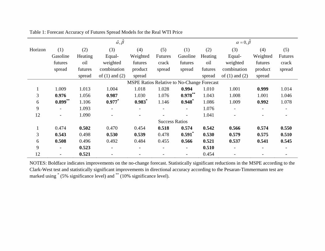
Table 1: Forecast Accuracy of Futures Spread Models for the Real WTI Price

ˆˆ , ˆ0, Horizon (1)

Gasoline futures spread

(2) Heating

oil futures spread

(3) Equal-

weighted combination of (1) and (2)

(4) Weighted

futures product spread

(5) Futures crack spread

(1) Gasoline futures spread

(2) Heating

oil futures spread

(3) Equal-

weighted combination of (1) and (2)

(4) Weighted

futures product spread

(5) Futures crack spread

MSPE Ratios Relative to No-Change Forecast 1 1.009 1.013 1.004 1.018 1.028 0.994 1.010 1.001 0.999 1.014 3 0.976 1.056 0.987 1.030 1.076 0.978** 1.043 1.008 1.001 1.046 6 0.899** 1.106 0.977* 0.983* 1.146 0.948* 1.086 1.009 0.992 1.078 9 - 1.093 - - - - 1.076 - - - 12 - 1.090 - - - - 1.041 - - - Success Ratios 1 0.474 0.502 0.470 0.454 0.518 0.574 0.542 0.566 0.574 0.550 3 0.543 0.498 0.530 0.539 0.478 0.591* 0.530 0.579 0.575 0.510 6 0.508 0.496 0.492 0.484 0.455 0.566 0.521 0.537 0.541 0.545 9 - 0.523 - - - - 0.510 - - - 12 - 0.521 - - - - 0.454 - - -

NOTES: Boldface indicates improvements on the no-change forecast. Statistically significant reductions in the MSPE according to the Clark-West test and statistically significant improvements in directional accuracy according to the Pesaran-Timmermann test are marked using * (5% significance level) and ** (10% significance level).

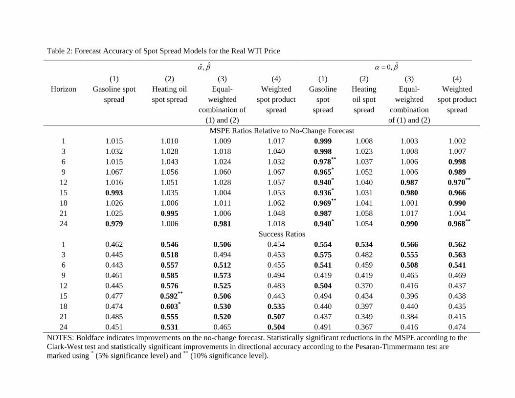
Table 2: Forecast Accuracy of Spot Spread Models for the Real WTI Price

ˆˆ , ˆ0,

Horizon (1)

Gasoline spot spread

(2) Heating oil spot spread

(3) Equal-

weighted combination of

(1) and (2)

(4) Weighted

spot product spread

(1) Gasoline

spot spread

(2) Heating oil spot spread

(3) Equal-

weighted combination of (1) and (2)

(4) Weighted

spot product spread

MSPE Ratios Relative to No-Change Forecast 1 1.015 1.010 1.009 1.017 0.999 1.008 1.003 1.002 3 1.032 1.028 1.018 1.040 0.998 1.023 1.008 1.007 6 1.015 1.043 1.024 1.032 0.978** 1.037 1.006 0.998 9 1.067 1.056 1.060 1.067 0.965* 1.052 1.006 0.989 12 1.016 1.051 1.028 1.057 0.940* 1.040 0.987 0.970**

15 0.993 1.035 1.004 1.053 0.936* 1.031 0.980 0.966 18 1.026 1.006 1.011 1.062 0.969** 1.041 1.001 0.990 21 1.025 0.995 1.006 1.048 0.987 1.058 1.017 1.004 24 0.979 1.006 0.981 1.018 0.940* 1.054 0.990 0.968**

Success Ratios 1 0.462 0.546 0.506 0.454 0.554 0.534 0.566 0.562 3 0.445 0.518 0.494 0.453 0.575 0.482 0.555 0.563 6 0.443 0.557 0.512 0.455 0.541 0.459 0.508 0.541 9 0.461 0.585 0.573 0.494 0.419 0.419 0.465 0.469 12 0.445 0.576 0.525 0.483 0.504 0.370 0.416 0.437 15 0.477 0.592** 0.506 0.443 0.494 0.434 0.396 0.438 18 0.474 0.603* 0.530 0.535 0.440 0.397 0.440 0.435 21 0.485 0.555 0.520 0.507 0.437 0.349 0.384 0.415 24 0.451 0.531 0.465 0.504 0.491 0.367 0.416 0.474

NOTES: Boldface indicates improvements on the no-change forecast. Statistically significant reductions in the MSPE according to the Clark-West test and statistically significant improvements in directional accuracy according to the Pesaran-Timmermann test are marked using * (5% significance level) and ** (10% significance level).

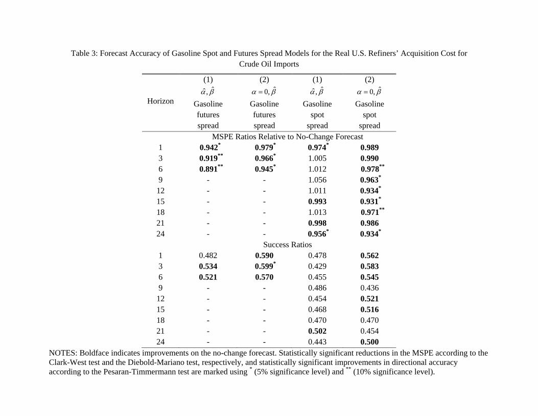
Table 3: Forecast Accuracy of Gasoline Spot and Futures Spread Models for the Real U.S. Refiners’ Acquisition Cost for Crude Oil Imports

(1) (2) (1) (2)

Horizon ˆˆ ,

Gasoline futures spread

ˆ0, Gasoline futures spread

ˆˆ , Gasoline

spot spread

ˆ0, Gasoline

spot spread

MSPE Ratios Relative to No-Change Forecast 1 0.942* 0.979* 0.974* 0.989 3 0.919** 0.966* 1.005 0.990 6 0.891** 0.945* 1.012 0.978**

9 - - 1.056 0.963*

12 - - 1.011 0.934*

15 - - 0.993 0.931*

18 - - 1.013 0.971**

21 - - 0.998 0.986 24 - - 0.956* 0.934*

Success Ratios 1 0.482 0.590 0.478 0.562 3 0.534 0.599* 0.429 0.583 6 0.521 0.570 0.455 0.545 9 - - 0.486 0.436 12 - - 0.454 0.521 15 - - 0.468 0.516 18 - - 0.470 0.470 21 - - 0.502 0.454 24 - - 0.443 0.500

NOTES: Boldface indicates improvements on the no-change forecast. Statistically significant reductions in the MSPE according to the Clark-West test and the Diebold-Mariano test, respectively, and statistically significant improvements in directional accuracy according to the Pesaran-Timmermann test are marked using * (5% significance level) and ** (10% significance level).

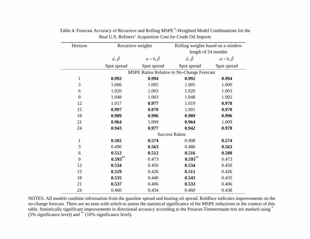
Table 4: Forecast Accuracy of Recursive and Rolling MSPE-1-Weighted Model Combinations for the Real U.S. Refiners’ Acquisition Cost for Crude Oil Imports

Horizon Recursive weights Rolling weights based on a window length of 24 months

ˆˆ , Spot spread

ˆ0, Spot spread

ˆˆ , Spot spread

ˆ0, Spot spread

MSPE Ratios Relative to No-Change Forecast 1 0.992 0.994 0.992 0.994 3 1.006 1.005 1.005 1.000 6 1.020 1.003 1.020 1.003 9 1.048 1.003 1.048 1.002 12 1.017 0.977 1.019 0.978 15 0.997 0.970 1.001 0.970 18 0.989 0.996 0.989 0.996 21 0.964 1.009 0.964 1.009 24 0.943 0.977 0.942 0.978

Success Ratios 1 0.502 0.574 0.498 0.574 3 0.490 0.563 0.486 0.563 6 0.512 0.512 0.516 0.508 9 0.593** 0.473 0.593** 0.473

12 0.534 0.450 0.534 0.450 15 0.519 0.426 0.511 0.426 18 0.535 0.440 0.543 0.435 21 0.537 0.406 0.533 0.406 24 0.460 0.434 0.460 0.438

NOTES: All models combine information from the gasoline spread and heating oil spread. Boldface indicates improvements on the no-change forecast. There are no tests with which to assess the statistical significance of the MSPE reductions in the context of this table. Statistically significant improvements in directional accuracy according to the Pesaran-Timmermann test are marked using * (5% significance level) and ** (10% significance level).

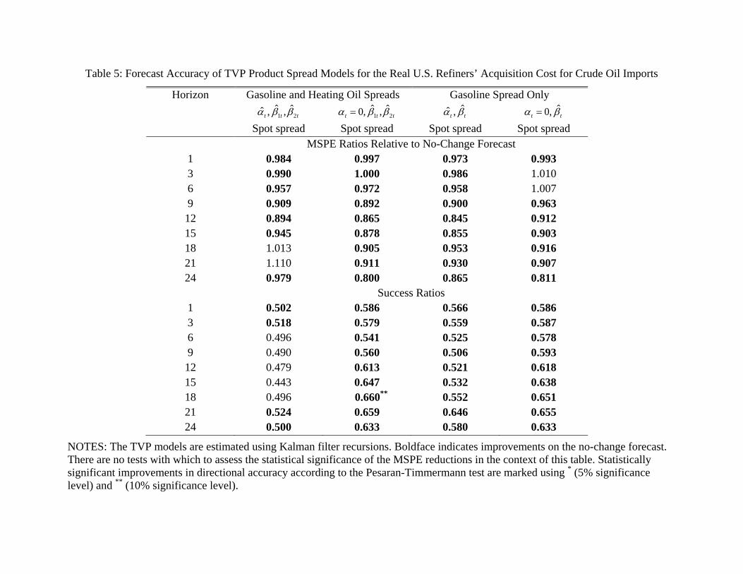
Table 5: Forecast Accuracy of TVP Product Spread Models for the Real U.S. Refiners’ Acquisition Cost for Crude Oil Imports

Horizon Gasoline and Heating Oil Spreads Gasoline Spread Only

1 2ˆ ˆˆ , ,t t t

Spot spread 1 2

ˆ ˆ0, ,t t t Spot spread

ˆˆ ,t t Spot spread

ˆ0,t t Spot spread

MSPE Ratios Relative to No-Change Forecast 1 0.984 0.997 0.973 0.993 3 0.990 1.000 0.986 1.010 6 0.957 0.972 0.958 1.007 9 0.909 0.892 0.900 0.963 12 0.894 0.865 0.845 0.912 15 0.945 0.878 0.855 0.903 18 1.013 0.905 0.953 0.916 21 1.110 0.911 0.930 0.907 24 0.979 0.800 0.865 0.811 Success Ratios 1 0.502 0.586 0.566 0.586 3 0.518 0.579 0.559 0.587 6 0.496 0.541 0.525 0.578 9 0.490 0.560 0.506 0.593 12 0.479 0.613 0.521 0.618 15 0.443 0.647 0.532 0.638 18 0.496 0.660** 0.552 0.65121 0.524 0.659 0.646 0.655 24 0.500 0.633 0.580 0.633

NOTES: The TVP models are estimated using Kalman filter recursions. Boldface indicates improvements on the no-change forecast. There are no tests with which to assess the statistical significance of the MSPE reductions in the context of this table. Statistically significant improvements in directional accuracy according to the Pesaran-Timmermann test are marked using * (5% significance level) and ** (10% significance level).

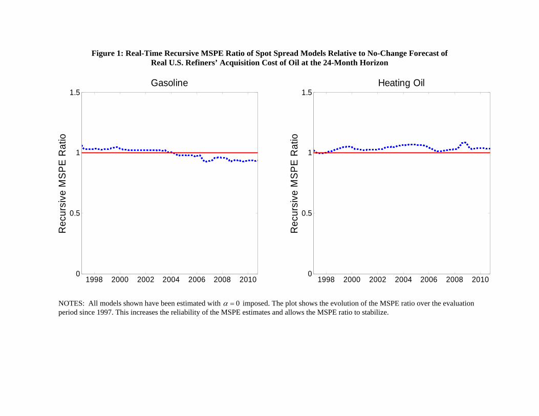
Figure 1: Real-Time Recursive MSPE Ratio of Spot Spread Models Relative to No-Change Forecast of Real U.S. Refiners’ Acquisition Cost of Oil at the 24-Month Horizon

1998 2000 2002 2004 2006 2008 20100

0.5

1

1.5

Rec

ursi

ve M

SPE

Rat

io

Gasoline

1998 2000 2002 2004 2006 2008 20100

0.5

1

1.5

Rec

ursi

ve M

SPE

Rat

io

Heating Oil

  NOTES: All models shown have been estimated with 0 imposed. The plot shows the evolution of the MSPE ratio over the evaluation period since 1997. This increases the reliability of the MSPE estimates and allows the MSPE ratio to stabilize.

NOT-FOR-PUBLICATION APPENDIX:

Are Product Spreads Useful for Forecasting? An Empirical

Evaluation of the Verleger Hypothesis

Christiane Baumeister Lutz Kilian∗

Bank of Canada University of Michigan

CEPR

Xiaoqing Zhou

University of Michigan

April 2014

This appendix provides additional results to demonstrate the robustness of our main findings.

1 Alternative inflation adjustment

To assess the robustness of our forecasts of the real price of oil to the adjustment for inflation, we

adapted the fixed-ρ inflation gap model proposed in Faust and Wright (2013) to generate monthly

out-of-sample inflation forecast. Table A1 shows that we obtain virtually identical results with this

alternative inflation adjustment as in our original approach.

2 Forecasts of the nominal oil price

Tables A2 and A3 show the results for forecasts of the nominal refiners’acquisition cost of imported

crude oil and of the nominal WTI spot price, respectively. The most successful forecasting models

are as accurate as or even more accurate than the corresponding real oil price forecasts, confirming

that the main results are not driven by our choice of inflation forecast.

∗Corresponding author: Lutz Kilian, University of Michigan, Department of Economics, 309 Lorch Hall, Ann

Arbor, MI 48109-1220. E-mail: lkilian@umich.edu.

1

3 Instabilities in the predictive relationship

Our results in the paper are based on recursive estimates of the forecasting models. An alternative

approach is to estimate forecasting models based on rolling windows of data. Table A4 evaluates

the accuracy of rolling forecasts of the real refiners’acquisition cost of crude oil imports based on

window lengths w ∈ {12, 24, 36}. The table shows that forecasts based on rolling windows performpoorly compared to recursive forecasts, regardless of the length of the window. Note that it is not

possible to increase w to 48 given the length of the initial sample size.

4 Additional figures

Figure A1 shows the popular 3:2:1 futures crack spread at the 3-month horizon for the period

January 1992 to March 2013. Figure A2 displays the time series behavior of selected product

spot spreads and 3-month product futures spreads. Figure A3 shows the evolution of the spread

between the WTI spot price and the Brent spot price over the period January 1992 to September

2012. Figure A4 plots the recursive MSPE ratios for the gasoline and heating oil spot spread models

at horizons h ∈ {6, 12, 18} starting in January 1997. It shows how robust the predictive relationshipis over time.

2

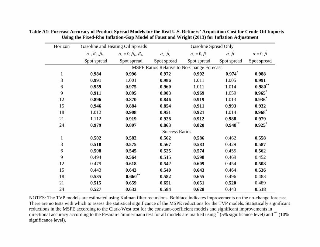
Table A1: Forecast Accuracy of Product Spread Models for the Real U.S. Refiners’ Acquisition Cost for Crude Oil Imports Using the Fixed-Rho Inflation-Gap Model of Faust and Wright (2013) for Inflation Adjustment

Horizon Gasoline and Heating Oil Spreads Gasoline Spread Only

1 2ˆ ˆˆ , ,t t t

Spot spread 1 2

ˆ ˆ0, ,t t t Spot spread

ˆˆ ,t t Spot spread

ˆ0,t t Spot spread

ˆˆ , Spot spread

ˆ0, Spot spread

MSPE Ratios Relative to No-Change Forecast 1 0.984 0.996 0.972 0.992 0.974* 0.988 3 0.991 1.001 0.986 1.011 1.005 0.991 6 0.959 0.975 0.960 1.011 1.014 0.980** 9 0.911 0.895 0.903 0.969 1.059 0.965* 12 0.896 0.870 0.846 0.919 1.013 0.936* 15 0.946 0.884 0.854 0.911 0.993 0.932 18 1.012 0.908 0.951 0.921 1.014 0.968* 21 1.112 0.919 0.928 0.912 0.988 0.979 24 0.979 0.807 0.863 0.820 0.948** 0.925*

Success Ratios 1 0.502 0.582 0.562 0.586 0.462 0.558 3 0.518 0.575 0.567 0.583 0.429 0.587 6 0.508 0.545 0.525 0.574 0.455 0.562 9 0.494 0.564 0.515 0.598 0.469 0.452 12 0.479 0.618 0.542 0.609 0.454 0.508 15 0.443 0.643 0.540 0.643 0.464 0.536 18 0.535 0.660** 0.582 0.655 0.496 0.483 21 0.515 0.659 0.651 0.651 0.520 0.489 24 0.527 0.633 0.584 0.628 0.443 0.518

NOTES: The TVP models are estimated using Kalman filter recursions. Boldface indicates improvements on the no-change forecast. There are no tests with which to assess the statistical significance of the MSPE reductions for the TVP models. Statistically significant reductions in the MSPE according to the Clark-West test for the constant-coefficient models and significant improvements in directional accuracy according to the Pesaran-Timmermann test for all models are marked using * (5% significance level) and ** (10% significance level).

Table A2: Forecast Accuracy of Product Spread Models for the Nominal U.S. Refiners’ Acquisition Cost for Crude Oil Imports

Horizon Gasoline and Heating Oil Spreads Gasoline Spread Only

1 2ˆ ˆˆ , ,t t t

Spot spread 1 2

ˆ ˆ0, ,t t t Spot spread

ˆˆ ,t t Spot spread

ˆ0,t t Spot spread

ˆˆ , Spot spread

ˆ0, Spot spread

MSPE Ratios Relative to No-Change Forecast 1 0.989 1.004 0.977 1.001 0.975** 0.992 3 0.997 1.008 0.993 1.022 1.005 0.996 6 0.959 0.976 0.960 1.019 1.014 0.983 9 0.902 0.884 0.894 0.971 1.059 0.960* 12 0.883 0.860 0.831 0.913 1.003 0.923* 15 0.909 0.866 0.823 0.895 0.971 0.908* 18 0.965 0.871 0.904 0.887 0.977 0.925* 21 1.041 0.872 0.868 0.864 0.936 0.916* 24 0.901 0.752 0.792 0.765 0.879* 0.855* Success Ratios 1 0.518 0.598 0.586 0.602 0.482 0.598 3 0.543 0.579 0.571 0.591 0.474 0.591 6 0.557 0.566 0.549 0.582 0.512 0.586 9 0.573 0.622 0.573 0.627 0.544 0.631 12 0.550 0.660** 0.605 0.651 0.521 0.651 15 0.545 0.664 0.604 0.668 0.511 0.668 18 0.599 0.668 0.672** 0.672 0.565 0.672 21 0.555 0.690 0.686 0.686 0.585 0.673 24 0.611 0.664 0.664 0.668 0.589 0.673

NOTES: The TVP models are estimated using Kalman filter recursions. Boldface indicates improvements on the no-change forecast. There are no tests with which to assess the statistical significance of the MSPE reductions for the TVP models. Statistically significant reductions in the MSPE according to the Clark-West test for the constant-coefficient models and significant improvements in directional accuracy according to the Pesaran-Timmermann test for all models are marked using * (5% significance level) and ** (10% significance level).

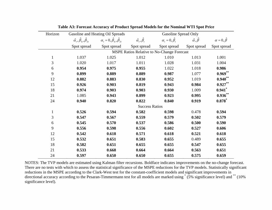
Table A3: Forecast Accuracy of Product Spread Models for the Nominal WTI Spot Price

Horizon Gasoline and Heating Oil Spreads Gasoline Spread Only

1 2ˆ ˆˆ , ,t t t

Spot spread 1 2

ˆ ˆ0, ,t t t Spot spread

ˆˆ ,t t Spot spread

ˆ0,t t Spot spread

ˆˆ , Spot spread

ˆ0, Spot spread

MSPE Ratios Relative to No-Change Forecast 1 1.037 1.025 1.012 1.010 1.013 1.001 3 1.020 1.017 1.011 1.028 1.031 1.004 6 0.954 0.975 0.955 1.022 1.018 0.986 9 0.899 0.889 0.889 0.987 1.077 0.969**

12 0.882 0.883 0.830 0.952 1.019 0.940** 15 0.926 0.903 0.819 0.943 0.984 0.927** 18 0.974 0.903 0.903 0.930 1.009 0.941* 21 1.085 0.943 0.899 0.923 0.995 0.936** 24 0.940 0.820 0.822 0.840 0.919 0.878*

Success Ratios 1 0.526 0.594 0.582 0.598 0.478 0.594 3 0.547 0.567 0.559 0.579 0.502 0.579 6 0.545 0.570 0.537 0.586 0.500 0.590 9 0.556 0.598 0.556 0.602 0.527 0.606 12 0.542 0.618 0.571 0.618 0.521 0.618 15 0.532 0.651 0.583 0.655 0.489 0.655 18 0.582 0.651 0.655 0.655 0.547 0.655 21 0.533 0.668 0.664 0.664 0.563 0.651 24 0.597 0.650 0.650 0.655 0.575 0.659

NOTES: The TVP models are estimated using Kalman filter recursions. Boldface indicates improvements on the no-change forecast. There are no tests with which to assess the statistical significance of the MSPE reductions for the TVP models. Statistically significant reductions in the MSPE according to the Clark-West test for the constant-coefficient models and significant improvements in directional accuracy according to the Pesaran-Timmermann test for all models are marked using * (5% significance level) and ** (10% significance level).

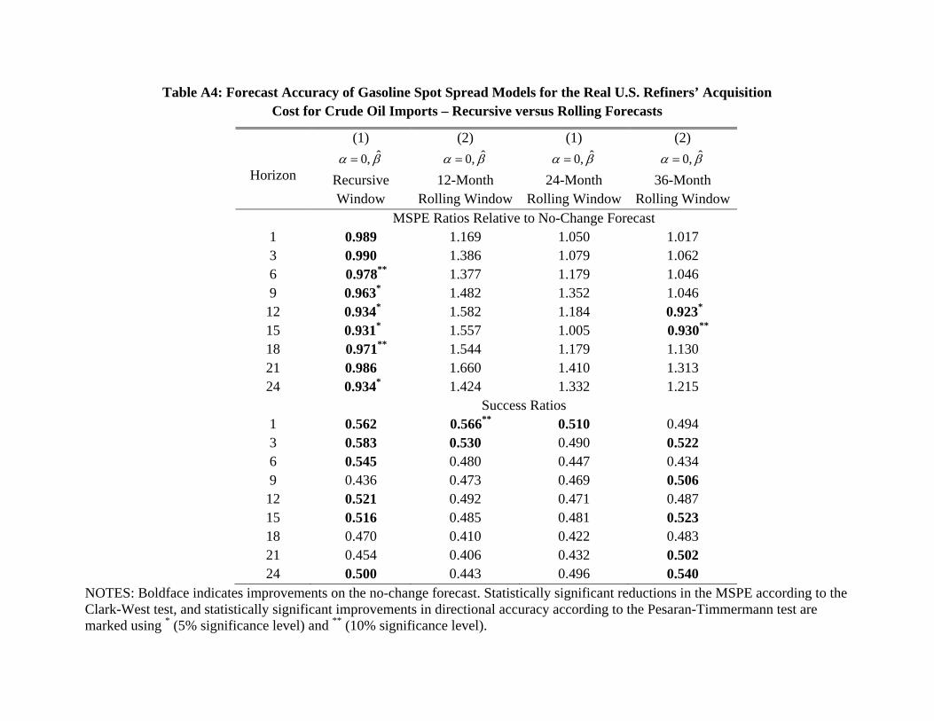
Table A4: Forecast Accuracy of Gasoline Spot Spread Models for the Real U.S. Refiners’ Acquisition Cost for Crude Oil Imports – Recursive versus Rolling Forecasts

(1) (2) (1) (2)

Horizon ˆ0,

Recursive Window

ˆ0, 12-Month

Rolling Window

ˆ0, 24-Month

Rolling Window

ˆ0, 36-Month

Rolling Window MSPE Ratios Relative to No-Change Forecast

1 0.989 1.169 1.050 1.017 3 0.990 1.386 1.079 1.062 6 0.978** 1.377 1.179 1.046 9 0.963* 1.482 1.352 1.046 12 0.934* 1.582 1.184 0.923* 15 0.931* 1.557 1.005 0.930** 18 0.971** 1.544 1.179 1.130 21 0.986 1.660 1.410 1.313 24 0.934* 1.424 1.332 1.215 Success Ratios 1 0.562 0.566** 0.510 0.494 3 0.583 0.530 0.490 0.522 6 0.545 0.480 0.447 0.434 9 0.436 0.473 0.469 0.506 12 0.521 0.492 0.471 0.487 15 0.516 0.485 0.481 0.523 18 0.470 0.410 0.422 0.483 21 0.454 0.406 0.432 0.502 24 0.500 0.443 0.496 0.540

NOTES: Boldface indicates improvements on the no-change forecast. Statistically significant reductions in the MSPE according to the Clark-West test, and statistically significant improvements in directional accuracy according to the Pesaran-Timmermann test are marked using * (5% significance level) and ** (10% significance level).

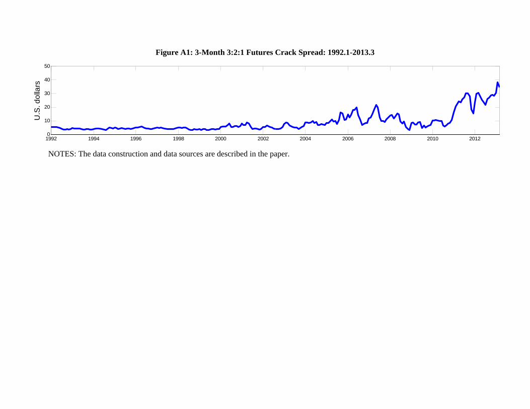
1992 1994 1996 1998 2000 2002 2004 2006 2008 2010 20120

10

20

30

40

50

U.S

. dol

lars

Figure A1: 3-Month 3:2:1 Futures Crack Spread: 1992.1-2013.3

NOTES: The data construction and data sources are described in the paper.

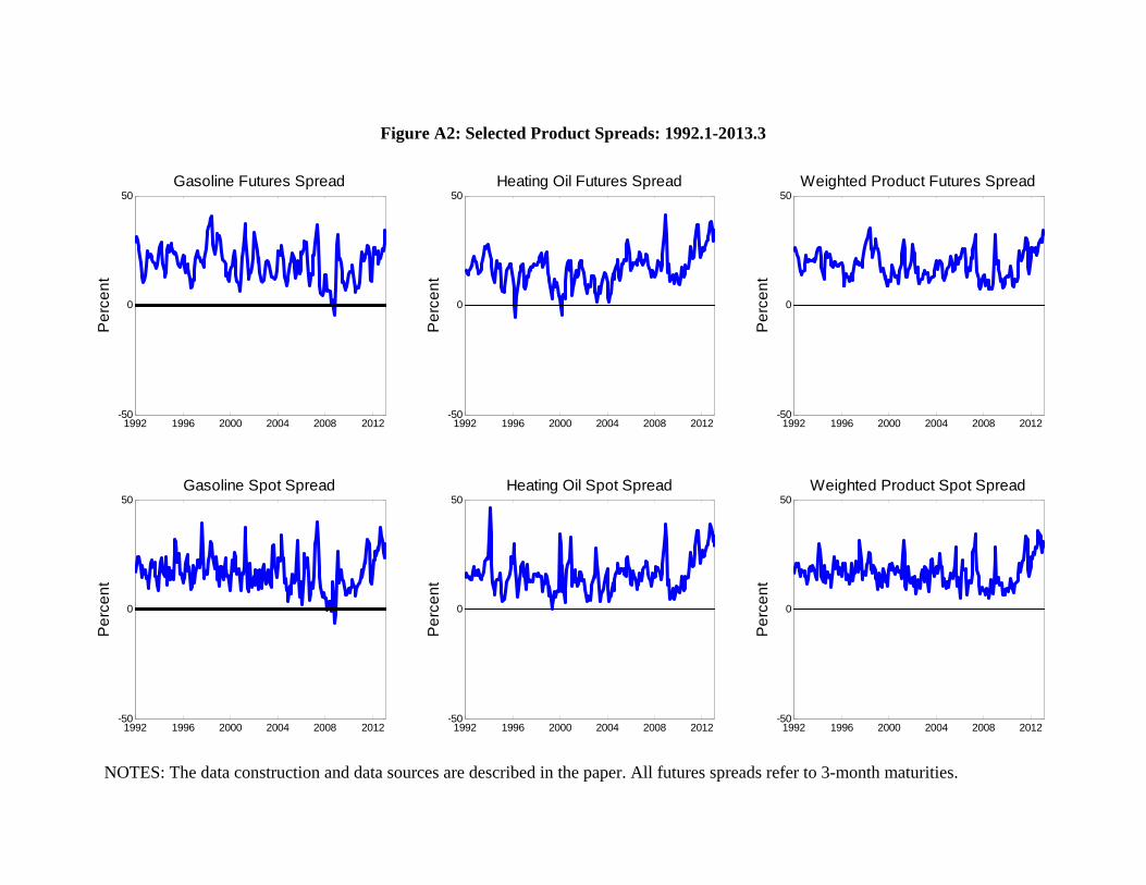
1992 1996 2000 2004 2008 2012-50

0

50Gasoline Futures Spread

Per

cent

1992 1996 2000 2004 2008 2012-50

0

50Heating Oil Futures Spread

Per

cent

1992 1996 2000 2004 2008 2012-50

0

50Weighted Product Futures Spread

Per

cent

1992 1996 2000 2004 2008 2012-50

0

50Gasoline Spot Spread

Per

cent

1992 1996 2000 2004 2008 2012-50

0

50Heating Oil Spot Spread

Per

cent

1992 1996 2000 2004 2008 2012-50

0

50Weighted Product Spot Spread

Per

cent

Figure A2: Selected Product Spreads: 1992.1-2013.3

NOTES: The data construction and data sources are described in the paper. All futures spreads refer to 3-month maturities.

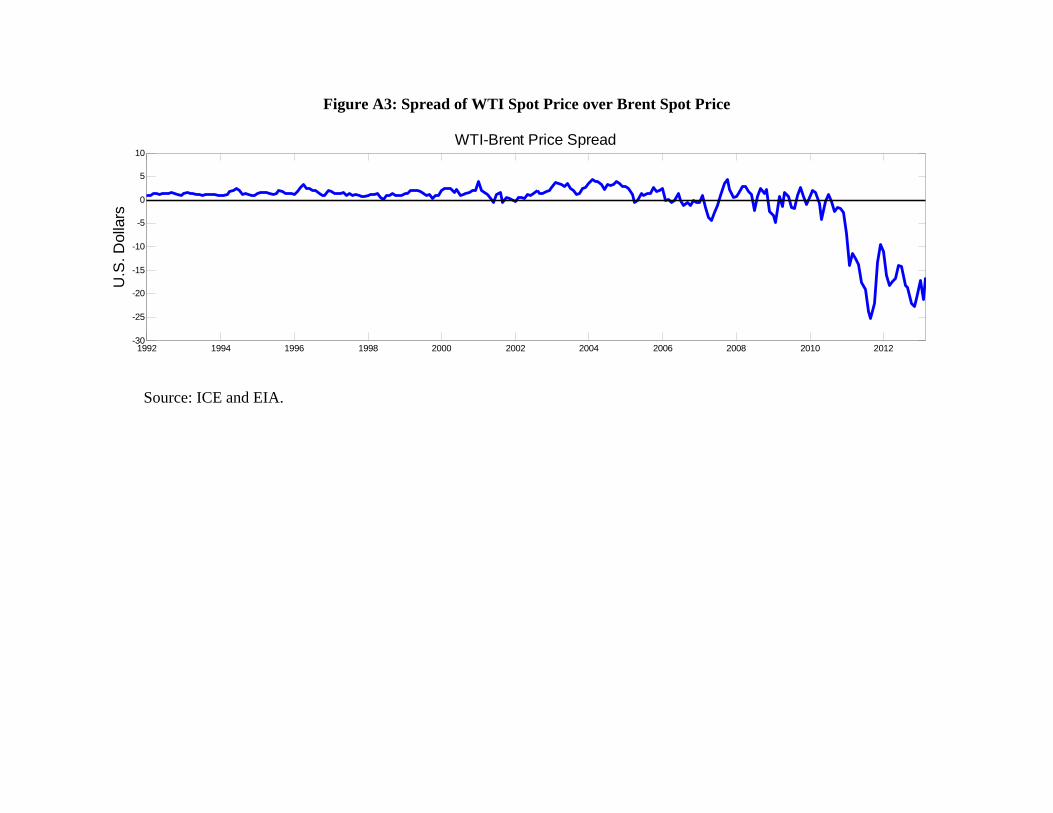
1992 1994 1996 1998 2000 2002 2004 2006 2008 2010 2012-30

-25

-20

-15

-10

-5

0

5

10WTI-Brent Price Spread

U.S

. Dol

lars

Figure A3: Spread of WTI Spot Price over Brent Spot Price

Source: ICE and EIA.

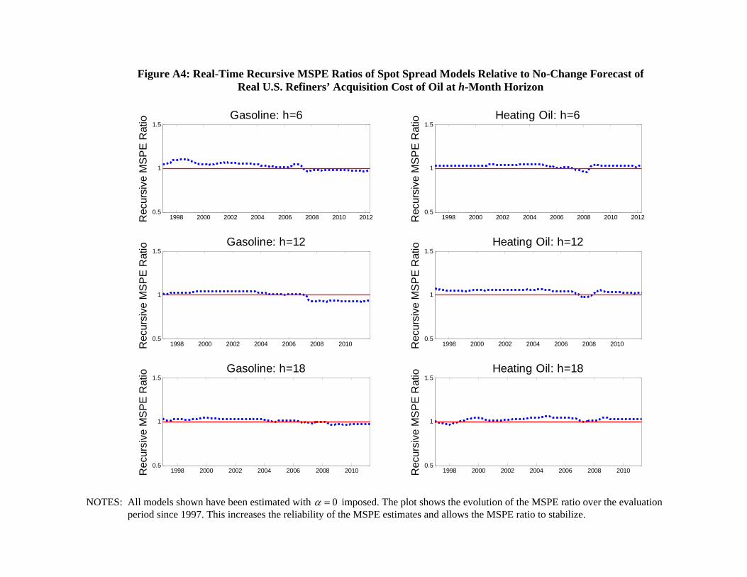
1998 2000 2002 2004 2006 2008 20100.5

1

1.5Gasoline: h=18

Rec

ursi

ve M

SP

E R

atio

1998 2000 2002 2004 2006 2008 20100.5

1

1.5Heating Oil: h=18

Rec

ursi

ve M

SP

E R

atio

1998 2000 2002 2004 2006 2008 20100.5

1

1.5Gasoline: h=12

Rec

ursi

ve M

SP

E R

atio

1998 2000 2002 2004 2006 2008 20100.5

1

1.5Heating Oil: h=12

Rec

ursi

ve M

SP

E R

atio

1998 2000 2002 2004 2006 2008 2010 20120.5

1

1.5Gasoline: h=6

Rec

ursi

ve M

SP

E R

atio

1998 2000 2002 2004 2006 2008 2010 20120.5

1

1.5Heating Oil: h=6

Rec

ursi

ve M

SP

E R

atio

Figure A4: Real-Time Recursive MSPE Ratios of Spot Spread Models Relative to No-Change Forecast of Real U.S. Refiners’ Acquisition Cost of Oil at h-Month Horizon

NOTES: All models shown have been estimated with 0 imposed. The plot shows the evolution of the MSPE ratio over the evaluation period since 1997. This increases the reliability of the MSPE estimates and allows the MSPE ratio to stabilize.