Forecasting interest rate swap spreads using domestic and international risk

factors: Evidence from linear and non-linear models

Ilias Lekkos

Department of Economic Analysis & Forecasting Eurobank - EFG, Greece

Costas Milas

School of Economic and Management Studies Keele University, UK

and

Theodore Panagiotidis*

Department of Economics Loughborough University, UK

March 2006

Abstract This paper explores the ability of factor models to predict the dynamics of US and UK interest rate swap spreads within a linear and a non-linear framework. We reject linearity for the US and UK swap spreads in favour of a regime-switching smooth transition vector autoregressive (STVAR) model, where the switching between regimes is controlled by the slope of the US term structure of interest rates. We compare the ability of the STVAR model to predict swap spreads with that of a non-linear nearest-neighbours model as well as that of linear AR and VAR models. We find some evidence that the non-linear models predict better than the linear ones. At short horizons, the nearest-neighbours (NN) model predicts better than the STVAR model US swap spreads in periods of increasing risk conditions and UK swap spreads in periods of decreasing risk conditions. At long horizons, the STVAR model increases its forecasting ability over the linear models, whereas the NN model does not outperform the rest of the models. Keywords: Interest rate swap spreads, term structure of interest rates, factor models, regime switching, smooth transition models, nearest-neighbours, forecasting. JEL classification: C51, C52, C53, E43. *Corresponding author: Dr Theodore Panagiotidis, Department of Economics, Loughborough University, Leicestershire LE11 3TU, Email: t.panagiotidis@lboro.ac.uk. We have benefited from the very useful comments and suggestions of an anonymous referee. We also thank Dick van Dijk for providing us with some of his routines in Gauss.

1

1. Introduction

The nature and identity of the risk factors that determine the spreads between the fixed-for-floating interest rate swaps and the underlying government bond yields have been examined by a number of researchers in both univariate and multivariate frameworks. Sun, Sundaresan and Wang (1993), Brown, Harlow and Smith (1994), Minton (1997) and Eom, Subrahmanyam and Uno (2001) examined whether factors such as the default-free interest rates and proxies for credit risk, liquidity risk and hedging costs can, within a univariate regression framework, account for the dynamics of interest rate swap spreads. Duffie and Singleton (1997) and Lekkos and Milas (2001) have extended the analysis of swap spreads to a multivariate vector autoregressive (VAR) framework. Duffie and Singleton (1997) find that default risk is significant in affecting longer maturity swap spreads. Lekkos and Milas (2001) examine the ability of factors such as the level, volatility and slope of the zero-coupon government bond yield curve, the TED spread (the difference between the 3-month LIBOR and the 3-month T-bill rate) and the corporate bond spread to describe the term structure of the US and UK swap spreads. They find that the slope of the term structure has a significant countercyclical effect across maturities, whereas the TED and corporate spreads play a smaller role and their significance varies across maturities. More recently, Lekkos and Milas (2004) and In (2005) examine in detail the issue of international linkages between interest rate swap markets.1 These links can be due to either common variations in the business cycles across economies or to coordinated arbitrage and hedging activities in the two markets.2 Lekkos and Milas (2004) employ non-linear smooth transition vector autoregressive (STVAR) models to show that the slope of the US term structure affects significantly swap spread dynamics in the UK. Similar findings are reported by In (2005), who employs multivariate VAR-EGARCH models to show that the slope of the US term structure has a significant effect on the Japanese and U.K. swap markets. Contrary to this plethora of studies on the identity of the factors affecting the dynamics of swap spreads, no previous study to our knowledge has attempted to forecast swap spreads out-of-sample. Our research uses a number of factors and functional forms, identified by previous studies, not to investigate the ability of these models to describe the in-sample behaviour of swap spreads, but to explore their out-of-sample forecasting performance. We adopt an international setting, where the term structures of the US and UK interest rate swap spreads depend upon the corporate bond spreads of the two countries, the interest rate differentials between the US and UK government bonds and the slopes (10 year rate minus 3-month T-Bill rate) of the term structures of the zero-coupon bond yields of the two countries. The corporate bond spreads are used as proxies for credit risk. The interest rate differentials are used to provide evidence of arbitrage trades between the two markets. The slopes of the term structure can be used to test whether the option to default is priced in swap markets; increases in the long-term interest rates imply that, during the first stages of the swap contract, the fixed rate will be higher than the expected short-term LIBOR. Therefore, the fixed-rate payer will be

1 Lekkos and Milas (2001) have provided some preliminary evidence on the impact of US factors on UK swap markets and Eom, Subrahmanyam and Uno (2001) on the links between US and Japanese swap markets. Fehle (2000) examines the impact that US swap spreads have on British, German, French, Japanese, Spanish and Dutch swap markets. 2 Lumsdaine and Prasad (1997) show that business cycles in each economy are not independent; instead they are affected, in different degrees, by a "world business cycle". Harvey (1991) finds that the correlation between the world and US business cycles is 87%.

2

exposed to the possibility of default of the floating-rate payer during the later stages of the contract. This exposure is priced in a higher swap spread. We assess the ability of these factors to forecast the US and UK interest rate swap spreads using both linear and non-linear models. Our linear specification consists of a VAR model, while the non-linear model we employ is a STVAR mode, which is an extension of the linear VAR to a regime switching framework, where the transition from one regime to the other occurs in a smooth way. The switching between regimes is controlled by an observed state variable. This feature of the STVAR model, that the transition from one regime to the other is a function of the underlying variables, allows us to test the ability of the different economic variables to best describe the non-linear dynamics of the term structure swap spreads.3 In order to assess whether the risk factors included and the functional forms assumed have any incremental value for forecasting the evolution of interest rate swap spreads, we also include in our forecasting horserace two more parsimonious and less structural models, a simple autoregressive model (AR) and a non-linear, non-parametric nearest neighbours model (NN). Contrary to the other models, which rely on global information in order to predict swap spreads, the NN model is a non-parametric local information model that uses a number of nearest neighbours to compute a weighted average estimate of swap spreads.4 The added flexibility of the NN models to capture the salient features of the data without the restrictions of a particular factor structure and functional form will provide a robust challenge to the performance and practical applications of the factor models. Our results indicate that, at short forecasting horizons, the flexibility of the atheoretic NN models is an advantage over all factor models and the AR specifications. However, the performance of the NN models decays rather quickly with the forecasting horizon. For longer horizon forecasts the STVAR specification provides the best forecasts, while the NN models ranks last. The structure of the paper is organised as follows. The next section describes the data. Sections 3 and 4 discuss the STVAR and NN models, respectively. Section 5 reports the forecasting results. Finally, section 6 concludes. 2. The data The data set consists of weekly observations from June 1991 to June 2001. We proxy the slope of the term structure of interest rates (denoted by USslope and UKslope, respectively) with the difference between the yields of the 10-year default-free zero-coupon bonds and the 3-month T-Bill rates. The US and UK zero-coupon yields are provided by the Bank of England. They are estimated by fitting a set of cubic splines to the prices of observed coupon-paying government bonds. The quality of the fit is controlled by a penalty function that restricts the curvature of the implied forward rates (see Anderson and Sleath, 1999). Zero-coupon yields are also used to estimate the difference between the 3-year, 7-year and 10-year US and UK interest rates, denoted by dif_3, dif_7 and dif_10, respectively. The US corporate spreads (denoted by UScorp) are estimated as the difference between Moody's AAA corporate bond yield index and the yields of the 10-year Treasury bonds. The UK corporate spread (denoted by UKcorp) is

3 Among other studies, Ang and Bekaert (2002), Bekaert, Hodrick and Marshall (2001), Hamilton (1988) and Gray (1996) use Hamilton’s (1989) Markov regime switching (MRS) model to explain the dynamics of short and long-term interest rates. In contrast to STVAR models, MRS models assume that an unobserved Markov state variable drives the switching between regimes. 4 Recent applications of NN models in finance include, e.g., Diebold and Nason (1990), Meese and Rose (1990), Gençay (1999), Jaditz and Riddick (2000), and Bajo-Rubio, Sosvilla-Rivero and Fernándes-Rodríguez (2001).

3

estimated as the difference between the corporate bond yield index provided by Datastream and the 10-year UK government bond yield. Finally, the US and UK swap spreads (denoted by USsp_i and UKsp_i, respectively, with i = 3, 7 and 10 years) are estimated as the difference between the bootstrapped5 zero-coupon swap rates and the corresponding maturity default-free zero-coupon rates. Figure 1 plots the US and UK swap spreads across maturities, whereas Table 1 reports the descriptive statistics for the US and UK swap spreads and the relevant risk factors. In both markets, swap spreads increase, on average, with maturity. Same maturity US and UK swap spreads are roughly equal but UK swap spreads are more volatile. The UK slope is also more volatile compared to the US slope. This can be explained by the fact that UK rates are, on average, higher than US rates over the sample period. Finally, the mean spread between US corporate and US treasury yields is 119 basis points and the corresponding UK corporate spread is 92 basis points. Preliminary analysis using Augmented Dickey-Fuller tests suggested that although all risk factors are stationary, the swap spreads are only borderline stationary. In line with earlier research in the area (e.g., Duffie and Singleton, 1997, and Lekkos and Milas, 2004), we proceed by treating the swap spreads as stationary series. 3. The Smooth Transition Vector Autoregressive (STVAR) model 3.1 The theoretical STVAR model We define a vector of state variables; one for each maturity we examine. For each maturity, this vector contains the relevant swap spreads as well as the US and UK term structure slopes, the difference between US and UK interest rates and the US and UK corporate spreads. We focus on the 3-year, 7-year and 10-year maturity swap spreads. For each of these maturities the vector of state variables is given by:

ty = [USslope, UKslope, dif_i, UScorp, UKcorp, USsp_i, UKsp_i]′ (1) where i = 3, 7 and 10 years. The corresponding STVAR model can be specified as: where yt is the (k x 1) vector defined above, Φ1,j and Φ2,j, j = 1,…, p, are (k x k) matrices, µ1 and µ2 are ( 1×k ) vectors, and εt ~ iid (0, Σ). G(st) is the transition function that controls the regime switching dynamics of yt. The STVAR model is a regime switching model where the transition between the two alternative regimes is controlled by the transition function G(.), which is continuous and bounded between 0 and 1. Values of zero identify one regime and values of unity identify the alternative and the transition between the two regimes occurs in a smooth way, i.e., the model does not allow jumps from one regime to the other. The regime that occurs at any time t is not probabilistic. Instead, it is determined by the transition variable ts and the

5 Bootstrapping is a particular methodology for extracting zero-coupon rates from interest rate swaps that trade at par. The transformation of the swap rates from par to zero-coupon is necessary in order for the swap rates to be comparable to government bond yields. For more details on the bootstrapping methodology see Appendix 1.

,)())(1(1

,221

,11 tt

p

jjtjt

p

jjtjt sGsG εyΦµyΦµy +⎟⎟

⎠

⎞⎜⎜⎝

⎛++−⎟⎟

⎠

⎞⎜⎜⎝

⎛+= ∑∑

=−

=− (2)

4

functional form of the transition function )( tsG . We focus our attention on the ‘logistic’ function: where σ (st) is the sample standard deviation of st. Model (3) allows for symmetric adjustment to positive and negative deviations of st relative to c. 6 The parameter c is the threshold between the two regimes, in the sense that G(st) changes monotonically from 0 to 1 as st increases, and takes the value of G(st) = 0.5 at cst = . The parameter γ determines the smoothness of the change in the value of the logistic function and thus the speed of the transition from one regime to the other. When γ → 0, the ‘logistic’ function equals a constant (i.e., 0.5), and when γ → + ∞, the transition from G(st) = 0 to G(st) = 1 is almost instantaneous at st = c. 3.2 Linearity testing in a STVAR model Testing for linearity in the STVAR model (2) using the ‘logistic’ transition model (3) is equivalent to testing the null hypothesis H0: γ = 0 against the alternative H1: γ > 0. To do this, define wt = (y1,t-1,…, y1,t-p, y2,t-1,…, y2,t-p,…, yk,t-1,…, yk,t-p) and assume that the transition variable (denoted by st) is known. Following Luukkonen, Saikkonen and Teräsvirta (1988), linearity testing equation by equation is based on a first-order Taylor approximation of the

transition function around γ = 0. We first estimate ∑=

++=pk

jitjtijiit wy

10 εββ and then use the

estimated residuals ite to run the following regression: ∑ ∑= =

+++=pk

jit

pk

jjttijtijiit wswe

1 10 ηδαα .

Denote the estimated residuals by vit. A Lagrange Multiplier (LM) test can be constructed as: LM = T (SSR0 – SSR1) / SSR0, where ∑= 2

0 iteSSR and ∑= 21 itvSSR . Under the null hypothesis

of linearity the LM statistic is distributed as a χ2(pk). In small samples, the χ2 test may be heavily oversized. Therefore, it is preferable to use the equivalent F version of the LM test statistic, which is given by F = [(SSR0 – SSR1) / pk] / [SSR1 / (T – (2pk + 1))]. It is well known that neglected heteroskedasticity may lead to spurious rejection of linearity. To tackle this problem, we use Wooldridge’s (1990, 1991) heteroskedasticity-robust versions of the tests. These tests can be used without having to specify the exact form of heteroskedasticity (see Granger and Teräsvirta, 1993). To compute a heteroskedasticity robust version of the LM test

statistic reported above, we first estimate ∑=

++=pk

jitjtijiit wy

10 εββ and save the estimated

residuals ite . We then regress the auxiliary regressors stwjt on wjt and save the residuals rjt. Finally, we regress 1 on ite rjt. The explained sum of squares from this last regression is the heteroskedasticity robust LM test statistic. Both the χ2 and F versions of the LM statistic are equation specific tests for linearity. To test the null hypothesis H0: γ = 0 in all equations simultaneously, we need a system-wide test. Following Weise (1999), define Tee tt /0 ∑ ′=Ω and Tvv tt /1 ∑ ′=Ω as the estimated variance-covariance residual matrices from the restricted and unrestricted estimated equations,

6 Leybourne, Sollis and Newbold (1999) consider smooth transition models with asymmetric adjustment.

,0,)](/)(exp[1),;( 1 >γσ−γ−+=γ −ttt scscsG (3)

5

respectively. Allowing for the standard finite sample LR correction, the log-likelihood system-wide test statistic is LR = (T – pk) 10 loglog Ω−Ω , which, under the null hypothesis of linearity is asymptotically distributed as χ2(pk2). 3.3 Empirical STVAR models 3.3.1 Linear VAR models and linearity testing We begin by estimating a benchmark linear VAR (one for each maturity) over “rolling” fixed-length windows of data, where the first data window runs from June 1991 until December 1998, and each successive data window is constructed by shifting the preceding window ahead by one week.7 Bearing in mind that a high-order VAR may cause over-fitting and make it more difficult to get converging estimates for the non-linear models, we use p = 2 lags in models (1). For each data window, we test for non-linearities and select the best candidate for the transition variable ts . We use all lagged variables in (1) as possible transition candidates st. To save space, Table 2 reports (for the first data window from June 1991 to December 1998) equation specific LM tests and system-wide LR linearity tests for the different transition variable candidates only in the case of the 3-year US and UK swap spread equations. 8 The common approach is to select the appropriate transition variable associated with the smallest p-value. The LM tests identify the first lag of the slope of the US term structure of interest rates as the most appropriate transition variable. The LR system tests indicate that all VAR equations react in a non-linear way not only to USslopet-1, but also to all other lagged variables in the system. However, the LR tests are less informative than the LM tests as the corresponding p-values are almost always equal to zero. Therefore, we proceed by using USslopet-1 as the transition variable across all equations. 9 The intuitive reason for this choice is related to the ability of the slope of the term structure to predict economic expansions and recessions; in particular, steep slopes tend to precede periods of economic expansion, whereas flat or negative slopes tend to indicate recessions (for more details see, e.g., the recent survey by Stock and Watson, 2003, and references therein). Our empirical choice is also consistent with the findings of Harvey (1991) who found that the US term structure is able to forecast real economic growth in the UK while Ang and Bekaert (2002) provided evidence that the US slope Granger-causes the UK term structure. 3.3.2 Estimation of STVAR models and regime identification As for the linear models, we estimate STVAR models for each “rolling” data window. In order to estimate the STVAR models, we follow Granger and Teräsvirta (1993) and Teräsvirta (1994) in scaling the ‘logistic’ function (3) by dividing it by the standard deviation of the transition variable σ(st), so that γ becomes a scale-free parameter. Doing so avoids slow convergence or overestimation associated with estimates of γ. Following from the above scaling, we set γ = 1 as a starting value and the sample mean of st as a starting value for the threshold c. At the same

7 After estimating our models for each “rolling” data window, we forecast one and twenty-six weeks ahead as discussed in more detail in section 5 below. 8 Detailed Tables with linearity tests for the remaining US and UK swap maturities are available on request. As for the 3-year swap maturities, these select USslopet-1 as the appropriate transition variable. See the discussion below. 9 Linearity test results for each successive data window are consistent with those reported here in the sense that USslopet-1 is chosen as the most appropriate transition variable.

6

time, the estimates of the linear VAR equations for the USsp_i and UKsp_i, (i = 3, 7, and 10) provide the starting values for the parameters in the STVAR model (2). The regime identification of our models is reported in Figure 2, which plots (for the first data window from June 1991 to December 1998) the value of the transition function estimated for the 3-year swap spreads system over time. The estimated transition function for the first data window is G(USslopet-1; γ, c) = 1 + exp[−10.528(USslopet-1 − 2.837) /σ(USslopet-1)]-1. The periods from June 1991 to December 1991 and from January 1995 to December 1998 are classified into the first regime, while the periods from January 1992 to June 1993 and from March 1994 to August 1994 are classified into the second regime (the period from July 1993 to February 1994 falls into more intermediate regimes). Notice, however, that the economic interpretation of the two regimes is not straightforward because they do not always coincide with periods of economic expansion and recession. Recall that the first regime, which corresponds to a flat term structure, should identify periods of economic recession, while the alternative regime should identify periods of economic expansion. Our regime classification captures the recession that ended in December 1991 and the subsequent recovery of the US economy. Nevertheless, the years from 1995 to 1998, which are classified into the first regime, were periods of significant economic expansion. This period is identified with the first regime because the US slope (see figure 2) started declining by the end of 1994 and continued to move downwards between 1995 and 1998, despite the fact that these were periods of robust economic growth. Bearing in mind that the relationship between changes in the term structure and subsequent changes in economic activity is probabilistic and that our sample does not contain a significant number of changes from expansion to recession (and vice versa), we cannot explore further the reasons for this apparent broken link between the term structure and economic activity. That said, the ability of our model to classify correctly the recession ending in 1991 is consistent with Estrella, Rodrigues and Schich (2000), who find that models using the US slope are stable when predicting recessions but become unstable when predicting output growth. To get a feeling of how the transition function G(USslopet-1; γ, c) for the 3-year swap spreads system shifts as the sample is “rolled through”, Figure 3 plots estimates of the parameters γ and c over the rolling period from January to December 1999 (that is, the first set of γ and c estimates refer to the rolling sample ending in the first week of January 1999, whereas the last set of γ and c estimates refer to the rolling sample ending in the last week of December 1999). The figure suggests reasonable stability for the estimates of the c parameter and more variability for the estimates of the γ parameter. 4. Nearest-neighbours (NN) model Contrary to the STVAR model, which relies on global information to address nonlinearity, the NN model is a non-parametric local information model that uses a number of nearest neighbours to compute a weighted average estimate of swap spreads. We only give a very brief summary of the nearest-neighbours model here; for a detailed discussion see ,e.g., Gençay (1999) and Jaditz and Riddick (2000). In order to estimate yt conditional on its history (yt-

1,…,yt-n), convert the time series process Ttty 1 = into n past history components of the form

),...,,( 11 +−−= ntttnt yyyy . The idea here is to take the most recent history available and then

7

retrieve the k nearest neighbours by searching over the set of all n histories. That is, in order to estimate yt conditional on the information available at t–1, compute the distance between the

vector ),...,,( 211 ntttnt yyyy −−−− = and its k nearest neighbours to derive the estimator iti

k

iy∑

=1λ ,

where tiλ are the k nearest-neighbour weights. These are calculated using the sup norm

iiyxmay = . 10 The optimal number of nearest-neighbours is determined by the minimum

Mean Squared Prediction Error (MSPE) achieved by regressing yt on all possible nearest neighbours. Relying on optimally chosen local information, as opposed to the global information used by the rest of the models employed in our paper, may prevent overfitting (see, e.g., Gençay, 1999). It should also be pointed out that the optimal number of nearest-neighbours changes as we estimate nearest-neighbours models for each “rolling” data window. 5. Forecasting analysis 5.1 Some theoretical issues on forecasting In order to assess the usefulness of the non-linear models, we carry out our forecasting exercise over “rolling” fixed-length windows of data, where the first data window runs from June 1991 until December 1998, and each successive data window is constructed by shifting the preceding window ahead by one week. Therefore, we re-estimate our models for each data window and then produce out-of-sample forecasts for the US and UK swap spreads over h = 1 and h = 26 weeks ahead. Generating dynamic out-of-sample forecasts from non-linear models is more complicated compared with generating forecasts from linear models as the expected value of a non-linear function is different from the function evaluated at the expected value of its argument (see, e.g., Granger and Teräsvirta 1993, and Franses and Van Dijk 2000, among others). We tackle this issue by adopting at each step of our forecasting exercise a bootstrap method where errors used at step h (h >1) are the average errors obtained from simulating the STVAR model at step h one thousand times. We compute out-of-sample forecasts from STVAR models, univariate NN models, linear VAR models and univariate autoregressive (AR) swap spread models.11 Forecasting performance is evaluated using the Mean Squared Prediction Error (MSPE) and the Mean Absolute Prediction Error (MAPE) criteria. Further, in order to see whether the non-linear models outperform the AR and VAR models, we employ the Diebold and Mariano (1995) test. This is computed by weighting the forecast loss differentials between two competing models equally, where the loss differential for observation t is given by dt ≡ [g(eit|t-h) – g(ejt|t-h)], where g (.) is a general function of forecast errors (e.g., MSPE or MAPE). The null hypothesis of equal accuracy of the forecasts of two competing models can be expressed in terms of their corresponding loss functions, E[g(eit|t-h)] = E[g(ejt|t-h)], or equivalently in terms of their loss differential, E[dt] = 0. Let

∑−++

+=

=11 hPR

hRttd

Pd denote the sample mean loss differential over t observations, such that there are P

out-of-sample point forecasts and R observations have been used for estimation. The Diebold-Mariano test statistic follows asymptotically the standard normal distribution: 10 Alternatively, one can use Euclidean distances. We use the sup norm because it is computationally less intensive. Jaditz and Riddick (2000) point out that the sup norm is not worse than the Euclidean one. 11 We use two lags for all AR swap spread equations except for the USsp_7 and USsp_10 equations, where three lags are used; lags are selected based on the Akaike Information Criterion.

8

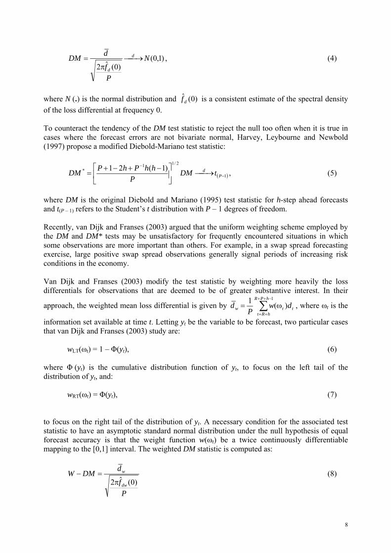
)1,0()0(ˆ2

N

Pf

dDM d

d

⎯→⎯π

= , (4)

where N (.) is the normal distribution and )0(ˆ

df is a consistent estimate of the spectral density of the loss differential at frequency 0. To counteract the tendency of the DM test statistic to reject the null too often when it is true in cases where the forecast errors are not bivariate normal, Harvey, Leybourne and Newbold (1997) propose a modified Diebold-Mariano test statistic:

( )1

2/11* )1(21

−

−

⎯→⎯⎥⎦

⎤⎢⎣

⎡ −+−+= P

d tDMP

hhPhPDM , (5)

where DM is the original Diebold and Mariano (1995) test statistic for h-step ahead forecasts and t(P – 1) refers to the Student’s t distribution with P – 1 degrees of freedom. Recently, van Dijk and Franses (2003) argued that the uniform weighting scheme employed by the DM and DM* tests may be unsatisfactory for frequently encountered situations in which some observations are more important than others. For example, in a swap spread forecasting exercise, large positive swap spread observations generally signal periods of increasing risk conditions in the economy. Van Dijk and Franses (2003) modify the test statistic by weighting more heavily the loss differentials for observations that are deemed to be of greater substantive interest. In their

approach, the weighted mean loss differential is given by ∑−++

+=

ω=1

)(1 hPR

hRtttw dw

Pd , where ωt is the

information set available at time t. Letting yt be the variable to be forecast, two particular cases that van Dijk and Franses (2003) study are:

wLT(ωt) = 1 – Φ(yt), (6) where Φ (yt) is the cumulative distribution function of yt, to focus on the left tail of the distribution of yt, and:

wRT(ωt) = Φ(yt), (7) to focus on the right tail of the distribution of yt. A necessary condition for the associated test statistic to have an asymptotic standard normal distribution under the null hypothesis of equal forecast accuracy is that the weight function w(ωt) be a twice continuously differentiable mapping to the [0,1] interval. The weighted DM statistic is computed as:

Pf

dDMWdw

w

)0(ˆ2π=− (8)

9

where )0(dwf is a consistent estimate of the spectral density of the loss differential at frequency 0. The weighted DM* test statistic is given by:

DMWP

hhPhPDMW −⎥⎦

⎤⎢⎣

⎡ −+−+=−

− 2/11* )1(21 (9)

Once again following Harvey et al. (1997), van Dijk and Franses (2003) propose using the Student's t distribution with P – 1 degrees of freedom to obtain critical values for the W–DM* test. In our forecasting exercise, the Left-tailed W-DM* statistic focuses on the ability of the competing models to forecast small swap spread values, which is interpreted as evidence of decreasing risk conditions in the economy. On the other hand, the Right-tailed W-DM* statistic focuses on the ability to forecast large spread values, which is interpreted as evidence of periods of increasing risk conditions in the economy. 5.2 Empirical results The results of our forecasting exercise are reported in Tables 3 and 4. We report the MSPE criteria for the different US and UK swap spread models (results using the MAPE criteria led to very similar conclusions and are available on request). The statistical significance of the forecasting performance of the non-linear STVAR and NN models relative to the linear VAR and AR models is examined using the modified DM*, Left-tailed W-DM* and Right-tailed W-DM* criteria. For both Tables 3 and 4, the top entry in [.] contains the p-values for the modified DM* statistic against the one-sided alternative that the MSPE of the competing model is lower. The middle entry in [.] contains the p-values for the modified Left-tailed W-DM* statistic while the bottom entry in [.] contains the p-values for the modified Right-tailed W-DM*. Table 3A reports the forecasting comparison over the short horizon of one week for the US. The 1-step ahead forecasts suggest that the NN model produces the lowest MSPE for two of the three US swap spread maturities. In particular, our results suggest forecasting superiority of the NN model over the AR, VAR and STVAR models for short and long US swap spread maturities (i.e. USsp_3 and USsp_10). However, the ability of the NN model to predict small spread values at the long end (i.e. USsp_10) is not better than that of the VAR model (p-value for the Left-tailed W-DM* equals 0.589) or that of the STVAR model (p-value for the Left-tailed W-DM* equals 0.144). The STVAR model does not beat the VAR model at any maturity, but it outperforms the AR model at the short maturity (i.e., USsp_3). For the 7-year US swap spread, the non-linear NN and STVAR models do not outperform the linear models. On the other hand, for the 7-year US swap spread, the NN model seems to outperform the STVAR model in predicting large swap spreads (p-value for the Right-tailed W-DM* equals 0.041). Table 3B reports the forecasting comparison over the longer horizon of six months. Contrary to our findings for the 1-step ahead forecasts, the 26-step ahead forecasts suggest that the STVAR model outperforms the VAR model for the short US maturity (i.e., USsp_3); further, the STVAR model outperforms the AR model for the long US maturity (i.e., USsp_10). Hence, there is evidence that the forecasting superiority of the STVAR model over the AR and VAR linear models increases at longer horizons. On the other hand, the forecasting ability of the NN model deteriorates over the longer horizon; in fact, the NN model fails to outperform the rest of the models. This is not surprising as the NN model is a local-information forecasting technique

10

which is only useful for short-term horizons (see, e.g., Jaditz and Sayers 1998, and Ramsey, 1996). Comparison of the 1-step ahead forecasts for the UK (see Table 4A) suggests that the NN model produces the lowest MSPE for two of the three UK swap spread maturities. In statistical terms, however, the NN model does not beat the AR model at any maturity. On the other hand, the NN model outperforms the linear VAR model at all maturities. Further, it outperforms the STVAR model at the 3-year and 7-year swap spread maturities. The NN model predicts small swap spread values better than the STVAR model at all maturities. The STVAR model outperforms the VAR model for short and long maturities. For the medium-to-long maturity swap spreads (i.e., the UKsp_7 swap spread), the STVAR model is able to predict better than the VAR model only small swap spread values (p-value for the Left-tailed W-DM* equals 0.004). Table 4B reports the forecasting comparison over the longer horizon of six months for the UK. Contrary to our findings for the 1-step ahead forecasts, the 26-step ahead forecasts suggest that the STVAR model outperforms the AR model for both short and long UK maturities (i.e. UKsp_3 and UKsp_10). On the other hand, the ability of the STVAR model to predict better than the VAR model does not improve (or worsen) over the longer horizon of 26 weeks. As in the US case, the NN model does not outperform any other model over the longer horizon. Overall, our forecasting exercise for the US and UK swap spreads suggests some forecasting superiority of non-linear models over linear ones. At the short horizon of 1 week, the NN non-linear model occasionally predicts better than the rest of the non-linear and linear models. At the longer horizon of 26 weeks, the STVAR model increases its forecasting ability over the linear models, whereas the NN model does not beat the rest of the models. Previous studies identified some superiority of the NN relative to other models. Gençay (1999) found that NN models outperform other linear and non-linear models for a number of exchange rates, whereas Bajo-Rubio, Sosvilla-Rivero and Fernándes-Rodríguez (2001) found evidence that NN models outperform linear models in predicting European interest rates. On the other hand, Teräsvirta, van Dijk and Medeiros (2005) used a number of G7 macroeconomic time series to show that STAR models forecast better when compared to linear models. 6. Conclusions Contrary to the majority of related research, this paper assesses the ability of both domestic and international risk factors to forecast, in an out-of-sample framework, the dynamics of the US and UK swap spreads. The forecasting performance of both linear and non-linear factor models is compared to the forecasts produced by more parsimonious, less structural models, such as a linear autoregressive (AR) model and a non-linear non-parametric nearest neighbourhood (NN) model. As far as the functional form of the factor model is concerned, we reject linearity in favour of a regime-switching STVAR model for the US and UK swap spread dynamics and we show that the switching between regimes is controlled by the slope of the US term structure of interest rates. The first regime is characterised by a "flat" term structure of US interest rates, while the alternative is characterised by an "upward" sloping US term structure. In economic terms, the two regimes do not always coincide with periods of economic expansion and recession. This can be interpreted as evidence of a break in the relationship between US real output growth and

11

the slope of the US term structure. We do not explicitly test for a break but possible reasons include the shift in US monetary policy from reactive to proactive as a response to the Asian and Russian financial crises and the Long-Term Capital Management (LTCM) collapse in 1998. Shifting our attention to the forecasting comparisons across models, we find that at short forecasting horizons, the flexibility of the atheoretic NN model provides an advantage over all factor STVAR and VAR models and the AR specification; the forecasting advantage of the NN over the STVAR model is more prominent for US swap spreads in periods of increasing risk conditions and for UK swap spreads in periods of decreasing risk conditions. On the other hand, the performance of the NN model decays rather quickly with the forecasting horizon. For longer horizon forecasts the STVAR specification increases its forecasting ability over the rest of the linear and non-linear models, while the NN model ranks last.

12

References

Anderson, N. and J. Sleath (1999). New estimates of the UK real and nominal yield curves, Bank of England Quarterly Bulletin, 39, 384-392.

Ang, A. and G. Bekaert (2002). Regime switches in interest rates. Journal of Business and

Economic Statistics 20, 163-182. Bajo-Rubio, O., Sosvilla-Rivero, S. and F. Fernándes-Rodríguez (2001). Asymmetry in the

EMS: New evidence based on non-linear forecasts. European Economic Review, 45 451-473.

Bekaert, G., R.J. Hodrick and D.A. Marshall (2001). "Peso Problem" explanations for term

structure anomalies. Journal of Monetary Economics, 48, 241-270. Brown, K., W.V. Harlow and D.J. Smith (1994). An empirical analysis of interest rates

swap spreads. Journal of Fixed Income 3, 61-78. Diebold, F.X. and R.S. Mariano (1995). Comparing predictive accuracy. Journal of

Business and Economic Statistics, 13, 253-263. Diebold, F.X. and J.A. Nason (1990). Nonparametric exchange rate prediction? Journal of

International Economics, 28, 315–322. Duffie D. and K.J. Singleton (1997). An econometric model of the term structure of interest-

rate swap yields. Journal of Finance, 52, 1287-1321. Eom, Y.H., M.G. Subrahmanyam and J. Uno (2001). Credit risk and the yen interest rate

swap market. Working Paper 042, Stern Business School, New York. Estrella, A., A.P. Rodrigues and S. Schich (2000). How stable is the predictive power of the

yield curve? Evidence from Germany and the United States. Federal Reserve Bank of New York, Staff Report 113.

Fehle, F. (2000). The components of interest rate swap spreads: Theory and international

evidence. Unpublished manuscript, University of South Carolina. Franses, P.H. and D. van Dijk (2000). Non-linear time series models in empirical finance.

Cambridge University Press, Cambridge. Gençay, R. (1999). Linear, non-linear and essential foreign exchange rate prediction with

simple technical trading rules. Journal of International Economics, 47, 91-107. Granger, C.W.J., and T. Teräsvirta (1993). Modelling nonlinear economic relationships.

Oxford University Press, Oxford. Gray, S.F. (1996). Modeling the conditional distribution of interest rates as a regime

switching process. Journal of Financial Economics, 42, 42-62.

13

Hamilton, J.D. (1988). Rational expectations econometric analysis of changes in regime: An investigation of the term structure of interest rates. Journal of Economic Dynamics and Control, 12, 385 - 423.

Hamilton, J.D. (1989). A new approach to the economic analysis of nonstationary time

series and the business cycle. Econometrica, 57, 357-384. Harvey, C.R. (1991). The term structure and world economic growth. Journal of Fixed

Income, June, pp. 7-19. Harvey, D., S. Leybourne and P. Newbold (1997). Testing the equality of prediction mean

squared errors. International Journal of Forecasting, 13, 281-291. In, F. (2005). Volatility spillovers across international swap markets: the U.S., Japan, and

the U.K. Journal of International Money and Finance (forthcoming). Jaditz, T. and C.L. Sayers (1998). Out-of-sample forecast performance as a test for

nonlinearity in time series, Journal of Business and Economic Statistics, 16, 110-117.

Jaditz, T. and L.A. Riddick (2000). Time-series near-neighbor regression. Studies in Nonlinear Dynamics and Econometrics, 4, 35-44.

Lekkos, I. and C. Milas (2004). Common risk factors in the US and UK interest rate swap

markets: Evidence from a non-linear vector autoregression approach. Journal of Futures Markets, 24, 221-250.

Lekkos, I. and C. Milas (2001). Identifying the factors that affect interest rate swap spreads:

some evidence from the US and the UK. Journal of Futures Markets, 21, 737-768. Leybourne, S., R. Sollis and P. Newbold (1999). Unit roots and asymmetric smooth

transitions. Journal of Time Series Analysis, 20, 671-77. Lumsadaine, R.L. and E.S. Prasad (1997). Identifying the common component in

international economic fluctuations, National Bureau of Economic Research, Working Paper 5984.

Luukkonen, R., P. Saikkonen and T. Teräsvirta (1988). Testing linearity against smooth

transition autoregressive models. Biometrika, 75, 491-499. Meese, R.A. and A.K. Rose (1990). Non-linear, nonparametric, nonessential exchange rate

estimation. American Economic Review, 80, 192-196. Minton, B.A. (1997). An empirical examination of basic valuation models for plain vanilla

U.S. interest rate swaps. Journal of Financial Economics, 44, 251-277. Ramsey, J.B. (1996). If nonlinear models cannot forecast, what use are they?, Studies in

Nonlinear Dynamics and Econometrics, 1, 65-86. Stock, J.H. and M.W. Watson (2003). Forecasting output and inflation: the role of asset

prices. Journal of Economic Literature 41, 788-829.

14

Sun, T.S., Sundaresan, S., Wang, C. (1993). Interest rate swaps - An empirical investigation.

Journal of Financial Economics 34, 77-99. Teräsvirta, T. (1994). Specification, estimation, and evaluation of smooth transition

autoregressive models. Journal of the American Statistical Association, 89, 208-218. Teräsvirta, T., D. van Dijk, and M.C. Medeiros (2005). Linear models, smooth transition

autoregressions, and neural networks for forecasting macroeconomic time series: A re-examination. International Journal of Forecasting, 21, 755-774.

van Dijk, D. and P.H. Franses (2003). Selecting a nonlinear time series model using

weighted tests of equal forecast accuracy. Oxford Bulletin of Economics and Statistics, 65, 727-744.

van Dijk, D., T. Teräsvirta, and P.H. Franses (2002). Smooth transition autoregressive

models – a survey of recent developments. Econometric Reviews, 21, 1-47. Weise, C.L. (1999). The asymmetric effects of monetary policy: a nonlinear vector

autoregression approach. Journal of Money, Credit, and Banking, 31, 85-108. Wooldridge, J.M. (1990). A unified approach to robust, regression-based specification tests.

Econometric Theory, 6, 17-43. Wooldridge, J.M. (1991). On the application of robust, regression-based diagnostics to

models of conditional means and conditional variances. Journal of Econometrics, 47, 5-46.

15

Table 1

Descriptive statistics

Mean Max Min Std. Dev Skewness Kurtosis

USsp_3 0.353 0.958 0.014 0.193 0.779 2.872 USsp_7 0.433 1.141 0.088 0.237 1.167 3.313 USsp_10 0.440 1.227 0.093 0.249 1.255 3.792

UKsp_3 0.333 1.010 0.002 0.217 0.634 2.358 UKsp_7 0.413 1.198 0.002 0.277 0.775 2.306 UKsp_10 0.466 1.280 0.003 0.302 0.910 2.635

USslope 1.581 4.141 0.690 1.182 0.382 2.139 UKslope 0.463 3.976 -2.669 1.619 0.196 1.704

Dif_3 -1.100 0.699 -5.294 1.097 -0.996 3.986 Dif_7 -0.813 1.087 -3.064 0.965 0.106 1.916 Dif_10 -0.591 1.323 -2.157 0.991 0.338 1.781 UScorp 1.196 2.150 0.630 0.346 0.759 2.804 UKcorp 0.920 2.068 0.015 0.418 0.257 2.422

Notes: The Table reports descriptive statistics for the swap spreads and the risk factors defined in section 2. The sample refers to weekly data from June 1991 to June 2001.

16

Table 2

Linearity tests for: ty = [USslope, UKslope, dif_3, UScorp, UKcorp, USsp_3, UKsp_3]′

Transition variable

USsp_3 equation

UKsp_3 equation

System test

USslopet-1 0.001 0.029 0.000 USslopet-2 0.006 0.039 0.000 UKslopet-1 0.037 0.497 0.001 UKslopet-2 0.093 0.585 0.004 Dif_3t-1 0.173 0.164 0.007 Dif_3t-2 0.155 0.107 0.006 UScorpt-1 0.382 0.092 0.000 UScorpt-2 0.401 0.054 0.002 UKcorpt-1 0.023 0.105 0.004 UKcorpt-2 0.030 0.206 0.090 USsp_3t-1 0.021 0.108 0.010 USsp_3t-2 0.037 0.266 0.020 UKsp_3t-1 0.288 0.197 0.030 Uksp_3t-2 0.334 0.088 0.050 Notes: The Table reports p-values of equation specific Lagrange Multiplier F statistics and system-wide LR test statistics for the USsp_3 and UKsp_3 equations. These are based on Wooldridge’s (1990, 1991) heteroskedasticity-robust versions of the tests. The null hypothesis is linearity. The alternative hypothesis is the STVAR model.

17

Table 3

Mean Squared Prediction Error (MSPE) for the US spreads using modified DM*, Left-tailed W-

DM* and Right-tailed W-DM*

(A) 1-step ahead forecasts MSPE p-values in [.]

STVAR NN VAR AR AR vs. STVAR

AR vs. NN

VAR vs. STVAR

VAR vs. NN STVAR vs. NN

USsp_3

0.160 0.049 0.135 0.166 [0.001]

[0.011] [0.000]

[0.000] [0.000] [0.000]

[0.999] [0.999] [0.999]

[0.000] [0.000] [0.000]

[0.000] [0.000] [0.000]

USsp_7

0.095 0.090 0.089 0.084 [0.997]

[0.995] [0.996]

[0.893] [0.974] [0.678]

[0.935] [0.996] [0.654]

[0.566] [0.970] [0.136]

[0.118] [0.515] [0.041]

USsp_10

0.105 0.077 0.095 0.085 [1.000]

[0.996] [1.000]

[0.048] [0.010] [0.001]

[0.999] [0.990] [0.999]

[0.000] [0.589] [0.000]

[0.000] [0.144] [0.000]

(B) 26-step ahead forecasts

MSPE p-values in [.] STVAR NN VAR AR AR vs.

STVAR AR vs. NN

VAR vs. STVAR

VAR vs. NN STVAR vs. NN

USsp_3

0.048 0.212 0.069 0.112 [0.000]

[0.000] [0.000]

[0.999] [0.954] [0.956]

[0.028] [0.013] [0.010]

[0.916] [0.944] [0.913]

[0.999] [0.999] [0.999]

USsp_7

0.144 0.198 0.074 0.113 [0.583]

[0.603] [0.621]

[0.936] [0.978] [0.931]

[0.945] [0.916] [0.694]

[0.999] [0.992] [0.993]

[0.921] [0.991] [0.992]

USsp_10

0.117 0.266 0.086 0.206 [0.000]

[0.000] [0.000]

[0.982] [0.923] [0.969]

[0.910] [0.885] [0.815]

[0.999] [0.999] [0.999]

[0.999] [0.999] [0.999]

Notes: MSPE for rolling window 1-step and 26-step ahead out-of sample forecasts from 1999:1 to 2001:26. The top entry in [.] contains the p-values for the modified DM* statistic of Harvey, Leybourne and Newbold (1997) against the one-sided alternative that the MSPE of the competing model is lower. The middle entry in [.] contains the p-values for the modified Left-tailed W-DM* statistic of van Dijk and Franses (2003). The bottom entry in [.] contains the p-values for the modified Right-tailed W-DM* statistic of van Dijk and Franses (2003).

18

Table 4

Mean Squared Prediction Error (MSPE) for the UK spreads using modified DM*, Left-tailed W-DM* and Right-tailed W-DM*

(A) 1-step ahead forecasts

MSPE p-values in [.] STVAR NN VAR AR AR vs.

STVAR AR vs. NN

VAR vs. STVAR

VAR vs. NN

STVAR vs. NN

UKsp_3

0.053 0.049 0.068 0.048 [0.998]

[0.999] [0.878]

[0.752] [0.990] [0.400]

[0.000] [0.000] [0.000]

[0.000] [0.000] [0.000]

[0.018] [0.021] [0.110]

UKsp_7

0.075 0.050 0.070 0.051 [1.000]

[0.999] [0.999]

[0.421] [0.384] [0.463]

[0.376] [0.004] [0.999]

[0.000] [0.000] [0.001]

[0.000] [0.000] [0.000]

UKsp_10

0.053 0.052 0.067 0.053 [0.549]

[0.923] [0.225]

[0.320] [0.369] [0.305]

[0.000] [0.000] [0.000]

[0.000] [0.000] [0.016]

[0.362] [0.043] [0.722]

(B) 26-step ahead forecasts

MSPE p-values in [.] STVAR NN VAR AR AR vs.

STVAR AR vs. NN

VAR vs. STVAR

VAR vs. NN STVAR vs. NN

UKsp_3

0.016 0.111 0.044 0.022 [0.031]

[0.000] [0.000]

[0.996] [0.991] [0.992]

[0.000] [0.000] [0.000]

[0.999] [0.789] [0.809]

[0.999] [0.999] [0.999]

UKsp_7

0.041 0.123 0.038 0.044 [0.344]

[0.221] [0.174]

[0.999] [0.993] [0.992]

[0.531] [0.003] [0.482]

[0.993] [0.992] [0.991]

[0.999] [0.999] [0.999]

UKsp_10

0.041 0.141 0.056 0.090 [0.000]

[0.000] [0.000]

[0.978] [0.921] [0.901]

[0.001] [0.000] [0.000]

[0.991] [0.934] [0.931]

[0.999] [0.999] [0.999]

Notes: MSPE for rolling window 1-step and 26-step ahead out-of sample forecasts from 1999:1 to 2001:26. The top entry in [.] contains the p-values for the modified DM* statistic of Harvey, Leybourne and Newbold (1997) against the one-sided alternative that the MSPE of the competing model is lower. The middle entry in [.] contains the p-values for the modified Left-tailed W-DM* statistic of van Dijk and Franses (2003). The bottom entry in [.] contains the p-values for the modified Right-tailed W-DM* statistic of van Dijk and Franses (2003).

19

Figure 1: 3, 7, and 10-year US and UK swap spreads

0

0.2

0.4

0.6

0.8

1

1.2

1.4

5-Jun-91 5-Jun-92 5-Jun-93 5-Jun-94 5-Jun-95 5-Jun-96 5-Jun-97 5-Jun-98 5-Jun-99 5-Jun-00 5-Jun-01

USspr3USspr7USspr10

0

0.2

0.4

0.6

0.8

1

1.2

1.4

5-Jun-91 5-Jun-92 5-Jun-93 5-Jun-94 5-Jun-95 5-Jun-96 5-Jun-97 5-Jun-98 5-Jun-99 5-Jun-00 5-Jun-01

UKspr3UKspr7UKspr10

20

Figure 2: Regime classification and the slope of the US term structure of interest rates

Notes: The figure plots the slope of the US term structure (solid line, right-hand axis, in percent) and the transition function for the 3-year swap spreads system (line with blocks, left-hand axis) over time. The transition function is estimated as: G(USslopet-1; γ, c) = 1 + exp[−10.528(USslopet-1 − 2.837) /σ(USslopet-1)]-1. Values of the transition function close to zero identify a period with the first regime while values of the transition function close to one identify a period with the second regime.

0

0.1

0.2

0.3

0.4

0.5

0.6

0.7

0.8

0.9

1

12-J

un-9

114

-Aug

-91

16-O

ct-9

129

-Jan

-92

15-A

pr-9

224

-Jun

-92

30-S

ep-9

230

-Dec

-92

3-M

ar-9

35-

May

-93

7-Ju

l-93

29-S

ep-9

31-

Dec

-93

9-Fe

b-94

13-A

pr-9

415

-Jun

-94

17-A

ug-9

426

-Oct

-94

4-Ja

n-95

22-M

ar-9

524

-May

-95

26-J

ul-9

54-

Oct

-95

6-D

ec-9

57-

Feb-

9610

-Apr

-96

19-J

un-9

628

-Aug

-96

30-O

ct-9

68-

Jan-

9712

-Mar

-97

14-M

ay-9

716

-Jul

-97

17-S

ep-9

719

-Nov

-97

28-J

an-9

81-

Apr-

983-

Jun-

985-

Aug-

987-

Oct

-98

9-D

ec-9

8

0

0.5

1

1.5

2

2.5

3

3.5

4

4.5

Transition function US SLOPE

21

Figure 3: Estimates of the transition function G(USslopet-1; γ, c) parameters for the 3-year swap spreads system over the rolling period from January to December 1999

(A) Estimates of the parameter γ over the rolling period from January to December 1999

1999 20005

10

15

20

25

30

35

40gamma

(B) Estimates of the parameter c over the rolling period from January to December 1999

1999 2000

1.8

2.0

2.2

2.4

2.6

2.8

3.0c

22

Appendix 1: Bootstrapping swap market data The most common type of interest rate swap is the fixed-to-floating par swap. This is a contract between two counterparties to exchange future cash flows or equivalently to exchange interest rate risk positions. One party of the swap, namely the fixed payer, agrees to pay on each payment day until the maturity of the swap an amount equal to a fixed interest rate applied on a notional principal. In return, the fixed payer receives from the other counterparty, the floating payer, cash flows based on the same notional principal but calculated with respect to a floating interest rate, e.g., LIBOR rate. The payments of these cash flows usually occur either annually or semi-annually. The technique used to infer the prices of zero-coupon bonds from swap rates is called bootstrapping and is based on the fact that interest rate swaps are par instruments with zero net present value. In the case of US dollar swaps, where the swap cash flows occur annually, the prices of discount bonds implied by the swap market are given by:

( )ttt

t

i iiitt s

bsb

,1

1

1 ,0,1,0 1

1

−

−

= −

+

−= ∑

αα

(A1) where ts is the swap rate, ti ,,2,1 …= and the accrual factor is ii ,1−α .12 The only problem is that swaps are available only for 2, 3, 4, 5, 7 and 10 years of maturity. Thus a linear interpolation has to be used to get an estimate of the missing swap rates. In the case of sterling swaps, where the swap cash flows occur semi-annually the calculations are slightly more complicated.13 If the swaps make semi-annual payments then we have to use swap rates every half a year in order to calculate the zero bond prices for the corresponding period. Again a linear interpolation has to be used to get an estimate of the missing swap rates. The only swap rate that we are not able to calculate using linear interpolation is the 5.1s swap rate as the one-year swap rate is not available and the corresponding one-year rate available from the money market is quoted on a different basis. As a result an adjustment has to be made:

1,01,5.05.0,05.0.0

1,011 bb

bs

αα +

−=

(A2) and 5.1s can be calculated by interpolating between 1s and 2s . Finally, the zero bond prices can be calculated using the bootstrap method as in equation (A1)

12 In the case of USD interest rate swaps the accrual factor is defined as

360

30,1 =− iiα .

13 In the case of GBP swap markets, the swap day-count convention is 365 days per year. Thus the accrual factor

is defined as 365

1,1

−−=−

ititiiα

.

23

but now the index i in the summation is being done semi-annually such that ti ,,5.2,2,5.1,1 …= . Based on those zero-coupon bond prices we can estimate the implied zero-coupon yields as 14

1

,0

,0

1,0 −

−

=⎟⎟

⎠

⎞

⎜⎜

⎝

⎛ t

tbtr

α

(A3)

14 The accrual factors now refer to bonds and are defined as

3651

,1−

−=

−i

ti

t

iiα .