Embed Size (px)
Citation preview
Are There Common Values in First-Price Auctions? A Tail-Index
Nonparametric Test
Appendix C: Additional Simulations
Jonathan B. Hill¤
Dept. of EconomicsUniversity of North Carolina -Chapel Hill
Artyom ShneyerovCIREQ, CIRANO and Concordia University, Montréal
September 2, 2012
In this appendix we replicate all simulations and the empirical study using the asymptotic
variance estimator ̂¡2for 90% con…dence bands ̂¡1
§164̂¡1
12 and t-statistics
12 (̂¡1
¡¡1)̂¡1
. We also present omitted simulation …gures for the cases of 2 f500 1000g auctions.
All simulation results verify the following: con…dence bands ̂¡1§ 164̂¡1
12 nearly per-
fectly match the empirical quantiles, and the t-ratio 12 (̂¡1
¡ ¡1)̂¡1under the null nearly
universally leads to over rejection of the null by a factor of 2-3 times. In particular, by using ̂¡2we
…nd under PV empirical size is roughly 10%-15% for a test with nominal size 5%. By comparisonif we use the kernel estimator ̂2j
empirical size is roughly 5% within a broad range of fractiles
. Under CV by using ̂¡2the range of fractiles for which the rejection rate is at of below
5% is roughly 1/3 to 1/2 the range obtained when using the kernel estimator ̂2j. Thus, for PV
data ̂2jconsistently leads to sharp size, and for CV data ̂2j
leads for a broader window offractiles on which empirical size is accurate (or over-rejection does not occur).
The reason for the poor performance of the test statistic 12 (̂¡1
¡¡1)̂¡1can be inferred
from the theory of CV and PV bids under out DGP, the simulation evidence itself, the followingdecomposition of 2j
shown in Section 3.3 of the main paper,
2j= ¡2 +
h()1
()2
jz
i£
(P=1 ( ¡ 1)
P=1
)
+ (1)
= ¡2 + [jz] + (1)
and the construction of ̂2j.
Since ()
is a linear function of tail arrays the covariance [()1
()2
jz] = (()2)
= () hence 2j= ¡2 + (1). See Section 3.3 and Appendix A.1 of the main paper. In
¤Dept. of Economics, University of North Carolina-Chapel Hill, www.unc.edu/»jbhill, [email protected].
1
small samples, however, [()1
()2
jz] 6= 0 with positive probability [wpp] is possible. Thisfollows since unobserved auction heterogeneity is likely to make bids positively associated withinthe auction (Krasnokutskaya 2010). Under CV by construction bids are positively associated dueto a¢liation, even when there is no unobserved heterogeneity, while heterogeneity is expected toinduce positive association even across PV bids in one auction. In order to understand why that
may imply [()1
()2
jz] 0 wpp, notice after invoking the moment properties presented inLemma 8 we have
h()1
()2
jz
i
» hn¡
ln¡
¤1
¢¢+
¡ ¡1³¤1
12
´on¡ln
¡
¤2
¢¢+
¡ ¡1³¤2
12
´ojz
i
This is asymptotically mean centered since by construction ¡1 (¤1
12 jz) ¼ ()¡1
and by Lemma 8 [(ln(¤1))+jz] ¼ ()¡1. Thus [
()1
()2
jz] 0 wpp with respectto a draw of positive auction sizes f : ¸ 1g if and only if normalized bids ¤1 and ¤2 in auction
tend to cluster: predominantly any two bids ¤1 ¤2
¡1 or ¤1 ¤2 ¸
¡1. Since ! 0 this implies bids tend either to cluster near the reserve price, or away from it, hence theyare positively associated. Therefore positive association in CV bids in general, and PV bids with
unobserved heterogeneity, may align with [()1
()2
jz] 0.
If [()1
()2
jz] 0 wpp holds then in general 2j ¡2 in small samples. This
in turn implies using ̂¡2to estimate 2j
can lead to systematic under-valuation of the truesmall sample mean-squared-error and therefore over-rejection of our test. Our simulation evidencestrongly supports this. Con…dence bands computed with ̂¡2
are tighter than those with ̂2j
because in general ̂¡2 ̂2j
, while use of ̂¡2leads to non-negligible over-rejection of either
null hypothesis. This suggests the sample version of [()1
()2
jz] that is implicitly computed
within ̂2jis positive wpp. Considering use of ̂2j
leads to a substantial improvement insharpness of our test statistic, employing an estimator that is robust to dependence in small samplesis preferred for …rst price auction data, in particular with unobserved heterogeneity.
Nevertheless, either test results in the same conclusion when applied to Canadian timber auc-tions: there is overwhelming evidence in favor of a CV strategy, and no evidence by any measurefor a PV strategy.
2
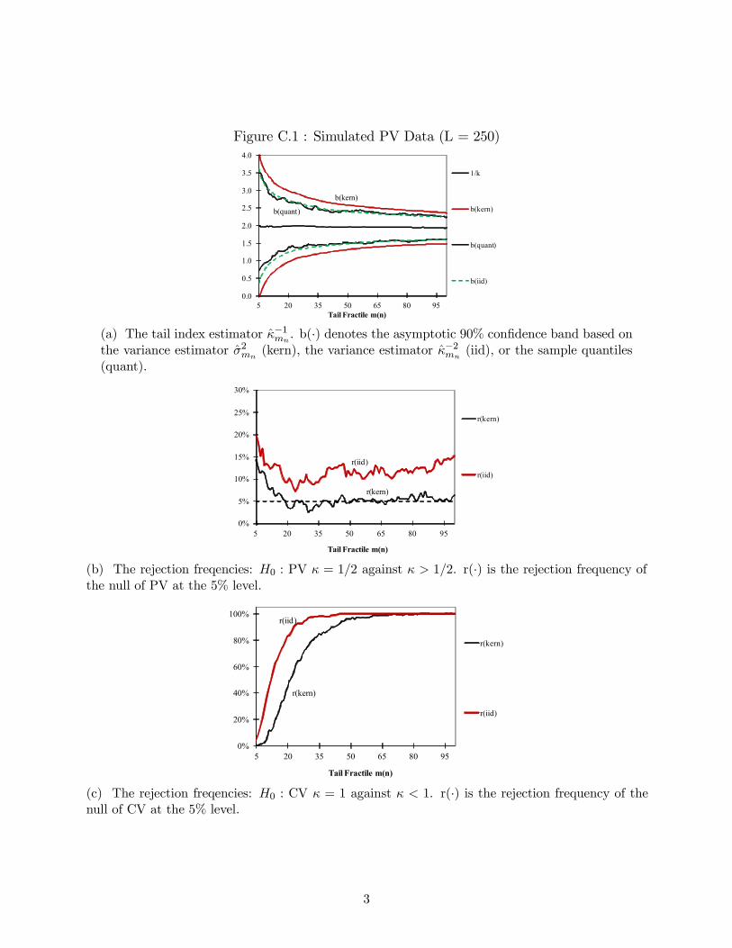
Figure C.1 : Simulated PV Data (L = 250)
b(kern)
b(quant)
0.0
0.5
1.0
1.5
2.0
2.5
3.0
3.5
4.0
5 20 35 50 65 80 95Tail Fractile m(n)
1/k
b(kern)
b(quant)
b(iid)
(a) The tail index estimator ̂¡1. b(¢) denotes the asymptotic 90% con…dence band based on
the variance estimator ̂2(kern), the variance estimator ̂¡2
(iid), or the sample quantiles(quant).
r(kern)
r(iid)
0%
5%
10%
15%
20%
25%
30%
5 20 35 50 65 80 95
Tail Fractile m(n)
r(kern)
r(iid)
(b) The rejection freqencies: 0 : PV = 12 against 12. r(¢) is the rejection frequency ofthe null of PV at the 5% level.
r(kern)
r(iid)
0%
20%
40%
60%
80%
100%
5 20 35 50 65 80 95
Tail Fractile m(n)
r(kern)
r(iid)
(c) The rejection freqencies: 0 : CV = 1 against 1. r(¢) is the rejection frequency of thenull of CV at the 5% level.
3
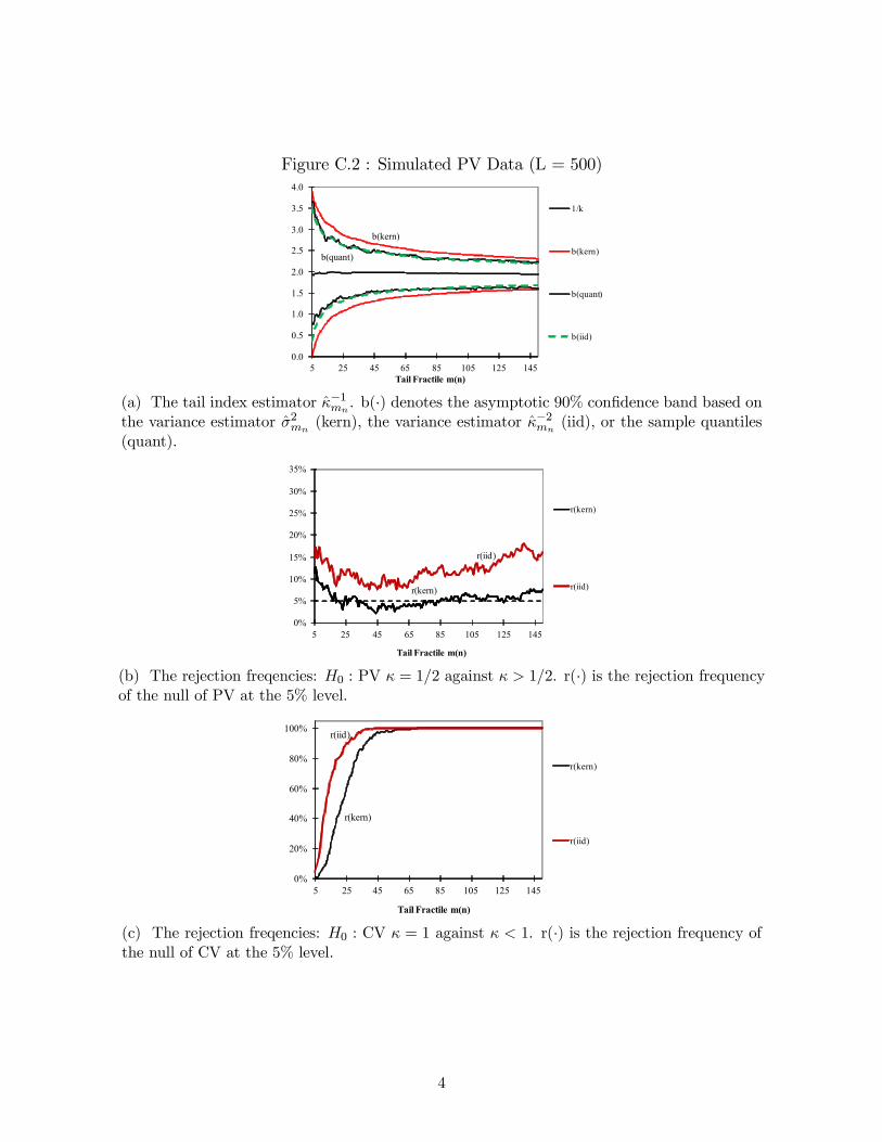
Figure C.2 : Simulated PV Data (L = 500)
b(kern)
b(quant)
0.0
0.5
1.0
1.5
2.0
2.5
3.0
3.5
4.0
5 25 45 65 85 105 125 145Tail Fractile m(n)
1/k
b(kern)
b(quant)
b(iid)
(a) The tail index estimator ̂¡1. b(¢) denotes the asymptotic 90% con…dence band based on
the variance estimator ̂2(kern), the variance estimator ̂¡2
(iid), or the sample quantiles(quant).
r(kern)
r(iid)
0%
5%
10%
15%
20%
25%
30%
35%
5 25 45 65 85 105 125 145
Tail Fractile m(n)
r(kern)
r(iid)
(b) The rejection freqencies: 0 : PV = 12 against 12. r(¢) is the rejection frequencyof the null of PV at the 5% level.
r(kern)
r(iid)
0%
20%
40%
60%
80%
100%
5 25 45 65 85 105 125 145
Tail Fractile m(n)
r(kern)
r(iid)
(c) The rejection freqencies: 0 : CV = 1 against 1. r(¢) is the rejection frequency ofthe null of CV at the 5% level.
4
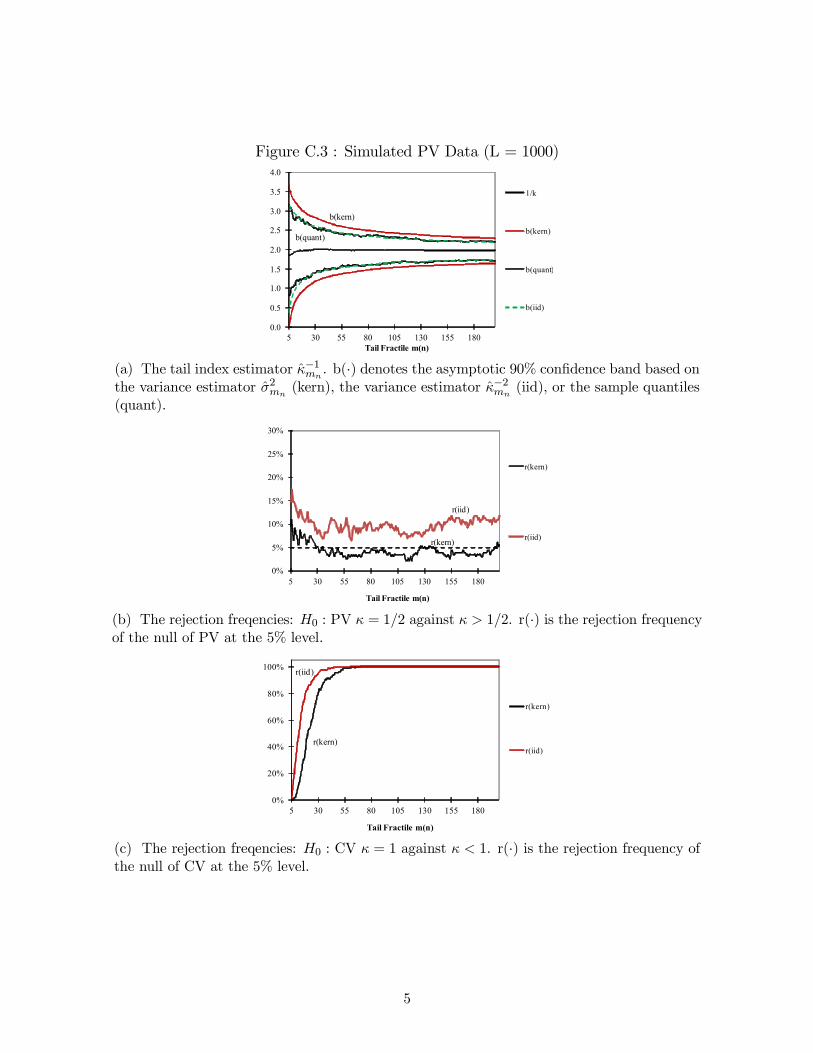
Figure C.3 : Simulated PV Data (L = 1000)
b(kern)
b(quant)
0.0
0.5
1.0
1.5
2.0
2.5
3.0
3.5
4.0
5 30 55 80 105 130 155 180Tail Fractile m(n)
1/k
b(kern)
b(quant)
b(iid)
(a) The tail index estimator ̂¡1. b(¢) denotes the asymptotic 90% con…dence band based on
the variance estimator ̂2(kern), the variance estimator ̂¡2
(iid), or the sample quantiles(quant).
r(kern)
r(iid)
0%
5%
10%
15%
20%
25%
30%
5 30 55 80 105 130 155 180
Tail Fractile m(n)
r(kern)
r(iid)
(b) The rejection freqencies: 0 : PV = 12 against 12. r(¢) is the rejection frequencyof the null of PV at the 5% level.
r(kern)
r(iid)
0%
20%
40%
60%
80%
100%
5 30 55 80 105 130 155 180
Tail Fractile m(n)
r(kern)
r(iid)
(c) The rejection freqencies: 0 : CV = 1 against 1. r(¢) is the rejection frequency ofthe null of CV at the 5% level.
5
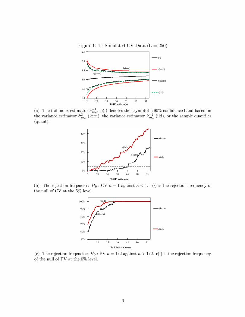
Figure C.4 : Simulated CV Data (L = 250)
b(kern)
b(quant)
0.0
0.5
1.0
1.5
2.0
2.5
5 20 35 50 65 80 95Tail Fractile m(n)
1/k
b(kern)
b(quant)
b(iid)
(a) The tail index estimator ̂¡1. b(¢) denotes the asymptotic 90% con…dence band based on
the variance estimator ̂2(kern), the variance estimator ̂¡2
(iid), or the sample quantiles(quant).
r(kern)
r(iid)
0%
10%
20%
30%
40%
5 20 35 50 65 80 95
Tail Fractile m(n)
r(kern)
r(iid)
(b) The rejection freqencies: 0 : CV = 1 against 1. r(¢) is the rejection frequency ofthe null of CV at the 5% level.
r(kern)
r(iid)
50%
60%
70%
80%
90%
100%
5 20 35 50 65 80 95
Tail Fractile m(n)
r(kern)
r(iid)
(c) The rejection freqencies: 0 : PV = 12 against 12. r(¢) is the rejection frequencyof the null of PV at the 5% level.
6
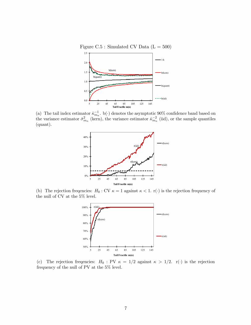
Figure C.5 : Simulated CV Data (L = 500)
b(kern)
b(quant)
0.0
0.5
1.0
1.5
2.0
2.5
5 25 45 65 85 105 125 145Tail Fractile m(n)
1/k
b(kern)
b(quant)
b(iid)
(a) The tail index estimator ̂¡1. b(¢) denotes the asymptotic 90% con…dence band based on
the variance estimator ̂2(kern), the variance estimator ̂¡2
(iid), or the sample quantiles(quant).
r(kern)
r(iid)
0%
10%
20%
30%
40%
5 25 45 65 85 105 125 145
Tail Fractile m(n)
r(kern)
r(iid)
(b) The rejection freqencies: 0 : CV = 1 against 1. r(¢) is the rejection frequency ofthe null of CV at the 5% level.
r(kern)
r(iid)
50%
60%
70%
80%
90%
100%
5 25 45 65 85 105 125 145
Tail Fractile m(n)
r(kern)
r(iid)
(c) The rejection freqencies: 0 : PV = 12 against 12. r(¢) is the rejectionfrequency of the null of PV at the 5% level.
7
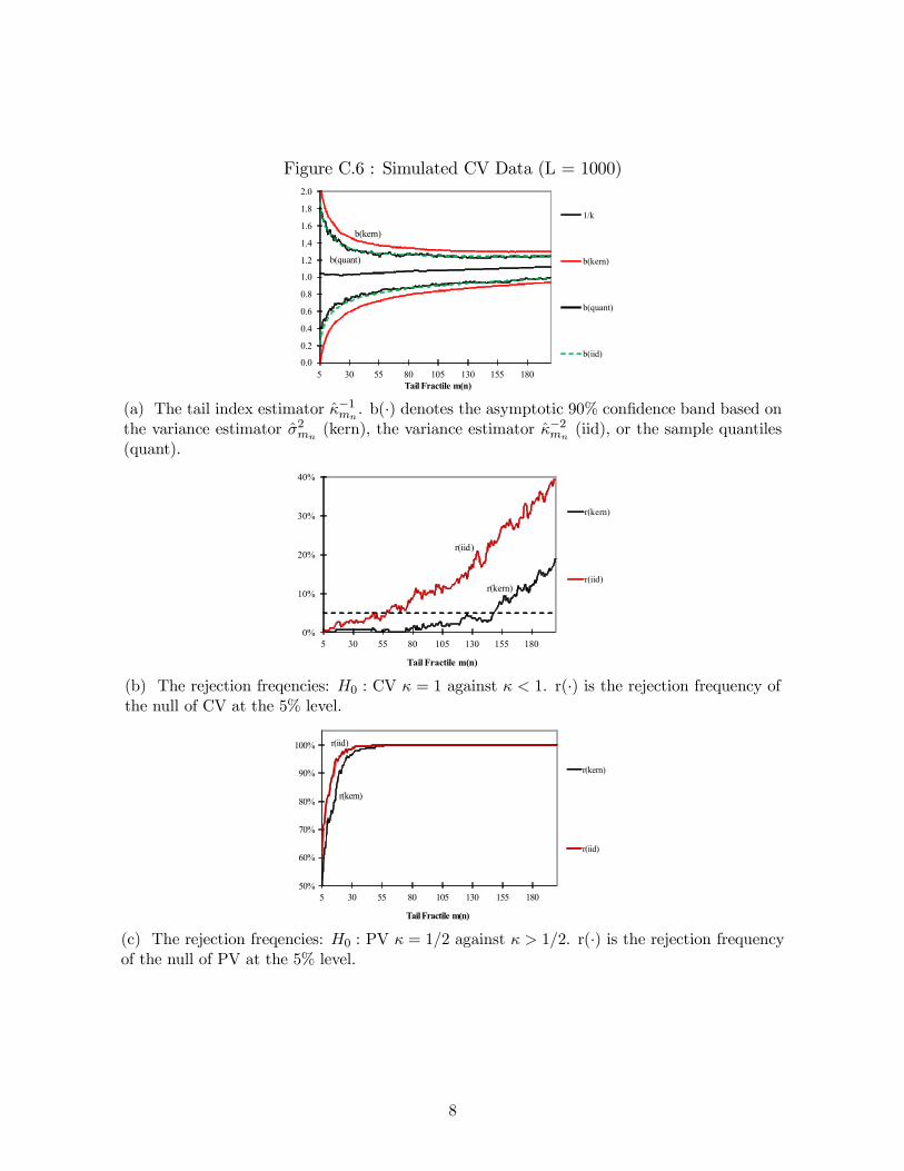
Figure C.6 : Simulated CV Data (L = 1000)
b(kern)
b(quant)
0.0
0.2
0.4
0.6
0.8
1.0
1.2
1.4
1.6
1.8
2.0
5 30 55 80 105 130 155 180Tail Fractile m(n)
1/k
b(kern)
b(quant)
b(iid)
(a) The tail index estimator ̂¡1. b(¢) denotes the asymptotic 90% con…dence band based on
the variance estimator ̂2(kern), the variance estimator ̂¡2
(iid), or the sample quantiles(quant).
r(kern)
r(iid)
0%
10%
20%
30%
40%
5 30 55 80 105 130 155 180
Tail Fractile m(n)
r(kern)
r(iid)
(b) The rejection freqencies: 0 : CV = 1 against 1. r(¢) is the rejection frequency ofthe null of CV at the 5% level.
r(kern)
r(iid)
50%
60%
70%
80%
90%
100%
5 30 55 80 105 130 155 180
TailFractile m(n)
r(kern)
r(iid)
(c) The rejection freqencies: 0 : PV = 12 against 12. r(¢) is the rejection frequencyof the null of PV at the 5% level.
8
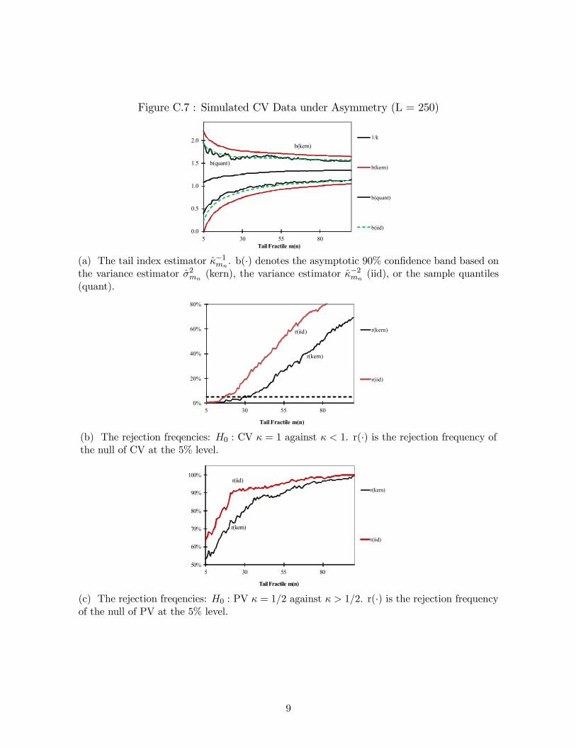
Figure C.7 : Simulated CV Data under Asymmetry (L = 250)
b(kern)
b(quant)
0.0
0.5
1.0
1.5
2.0
5 30 55 80Tail Fractile m(n)
1/k
b(kern)
b(quant)
b(iid)
(a) The tail index estimator ̂¡1. b(¢) denotes the asymptotic 90% con…dence band based on
the variance estimator ̂2(kern), the variance estimator ̂¡2
(iid), or the sample quantiles(quant).
r(kern)
r(iid)
0%
20%
40%
60%
80%
5 30 55 80
Tail Fractile m(n)
r(kern)
r(iid)
(b) The rejection freqencies: 0 : CV = 1 against 1. r(¢) is the rejection frequency ofthe null of CV at the 5% level.
r(kern)
r(iid)
50%
60%
70%
80%
90%
100%
5 30 55 80
TailFractile m(n)
r(kern)
r(iid)
(c) The rejection freqencies: 0 : PV = 12 against 12. r(¢) is the rejection frequencyof the null of PV at the 5% level.
9
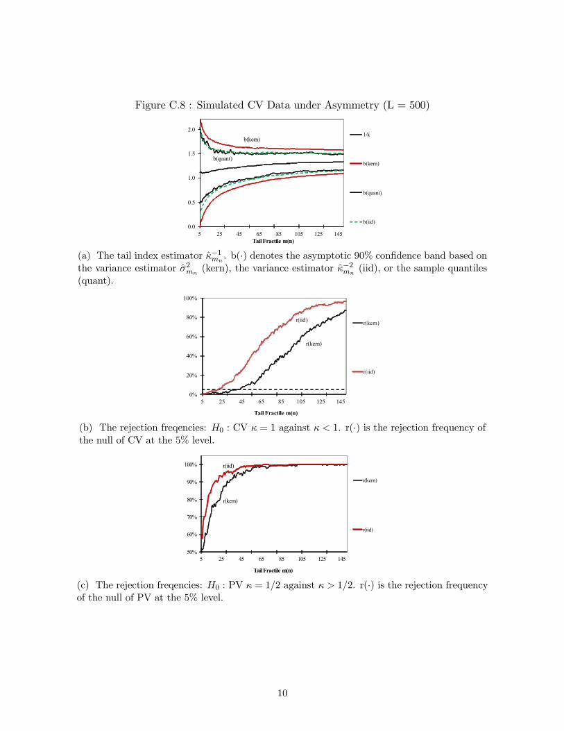
Figure C.8 : Simulated CV Data under Asymmetry (L = 500)
b(kern)
b(quant)
0.0
0.5
1.0
1.5
2.0
5 25 45 65 85 105 125 145Tail Fractile m(n)
1/k
b(kern)
b(quant)
b(iid)
(a) The tail index estimator ̂¡1. b(¢) denotes the asymptotic 90% con…dence band based on
the variance estimator ̂2(kern), the variance estimator ̂¡2
(iid), or the sample quantiles(quant).
r(kern)
r(iid)
0%
20%
40%
60%
80%
100%
5 25 45 65 85 105 125 145
Tail Fractile m(n)
r(kern)
r(iid)
(b) The rejection freqencies: 0 : CV = 1 against 1. r(¢) is the rejection frequency ofthe null of CV at the 5% level.
r(kern)
r(iid)
50%
60%
70%
80%
90%
100%
5 25 45 65 85 105 125 145
TailFractile m(n)
r(kern)
r(iid)
(c) The rejection freqencies: 0 : PV = 12 against 12. r(¢) is the rejection frequencyof the null of PV at the 5% level.
10

Figure C.9 : Simulated CV Data under Asymmetry (L = 1000)
b(kern)
b(quant)
0.0
0.5
1.0
1.5
2.0
5 30 55 80 105 130 155 180Tail Fractile m(n)
1/k
b(kern)
b(quant)
b(iid)
(a) The tail index estimator ̂¡1. b(¢) denotes the asymptotic 90% con…dence band based on
the variance estimator ̂2(kern), the variance estimator ̂¡2
(iid), or the sample quantiles(quant).
r(kern)r(iid)
0%
10%
20%
30%
40%
50%
60%
70%
5 30 55 80 105 130 155 180
Tail Fractile m(n)
r(kern)
r(iid)
(b) The rejection freqencies: 0 : CV = 1 against 1. r(¢) is the rejection frequency ofthe null of CV at the 5% level.
r(kern)
r(iid)
50%
60%
70%
80%
90%
100%
5 30 55 80 105 130 155 180
TailFractile m(n)
r(kern)
r(iid)
(c) The rejection freqencies: 0 : PV = 12 against 12. r(¢) is the rejection frequencyof the null of PV at the 5% level.
11
Figure C.10 : BCTS: tail index test
0.0
0.4
0.8
1.2
1.6
2.0
5 25 45 65 85 105 125 145 165 185Tail Fractile m(n)
1/k
b(kern)
b(iid)
(a) Co…dence bands b(¢) computed from the kernel estimator ̂2(kern) and from the variance
estimator ̂¡2(iid).
p(kern)
-0.001
0.001
0.002
0.003
0.004
5 25 45 65 85 105 125 145 165 185
Tail Fractile m(n)
p(kern)
p(iid)
(b) P-values for the t-test of PV = 1/2 on BCTS data.
p(kern)
0.0
0.1
0.2
0.3
0.4
0.5
0.6
5 25 45 65 85 105 125 145 165 185
Tail Fractile m(n)
p(kern)
p(iid)
(c) P-values for the t-test of CV = 1 on BCTS data.
12